Atomic Coherent States and Sphere Maps

Robert Gilmore

Physics Department, Drexel University, Philadelphia, Pennsylvania 19104, USA

(Dated: November 11, 2011)

An atomic coherent state will evolve to an atomic coherent state under a classical driving field.Under a time-periodic driving field the phase space for the dynamics is S2

×S1, so that chaotic

motion is possible. We explore the types of motion that can occur for periodically driven atomiccoherent states by investigating the properties of the first return map S

2→ S

2. The spheremap that we introduce is a generalization of the Kolmogorov-Arnold circle map that is based onthe Gauss sphere map. We find mixtures of mode-locking, quasiperiodicity, forward and reverseperiod-doubling cascades, and chaos.

I. INTRODUCTION

Atomic coherent states were initially introduced to describe the coherence properties of atoms in a laser cavity [1].The hamiltonian used to describe the interacting atom-field system in the laser cavity is

H =∑

k

hω(k)(a†kak +

1

2) +

∑

j

ǫ

2σzj +

∑

k

∑

j

(

λ∗(k)a†kσ−j e−ik·rj + λ(k)akσ

+j e

ik·rj)

(1)

In this expression a(k)† is the operator creating a photon of wave vector k and energy hω(k), j indexes the individualatoms, for which only two levels are assumed to be important in laser processes, rj is the position of the jth atomand the energy difference between the two atomic levels in the absence of fields is ǫ. The Pauli spin operator σz

j

describes the zero-field eigenstates of the jth atom, the interaction term λ∗(k)a†kσ−j describes the emission of a

photon of wavenumber k and the deexcitation of the jth atom, while λ(k)akσ+j describes photon absorption and

atomic excitation. It is usually assumed that there are N atoms and they are localized within a distance d overwhich the phases e±ik·rj do not vary significantly. The usual commutation relations apply:

[

σzj , σ

±k

]

= ±σ±j δjk,

[

ak, a†k′

]

= δk,k′I. Polarization indices have been suppressed.

II. TWO SEMICLASSICAL THEOREMS

Equation (1) has two dual semiclassical limits. In one limit the atomic sources are assumed to be classical, sothat the field is driven by a classical current. In this limit the sums over atoms can be replaced by classical currents∑

j σ±,zj → j(t)±,z and Eq. (1) can be replaced by the semiclassical limit

Hs.c. field =∑

k

hω(k)(a†kak +

1

2) + jz(t) +

∑

k

(

λ∗(k)a†kj−(t) + λ(k)akj

+(t))

(2)

where jz(t) is real and (j−(t))∗ = j+(t). In this case the classical current produces a coherent field state [2, 3, 4, 5].More specifically, if the field is initially in its ground state (no photons) then it will evolve into a field coherent statefor all future times.In the other limit the field is assumed to be classical, so that the field operators can be replaced by their expectation

values∑

ka(k)† → f∗(t), and in this limit the semiclassical hamiltonian takes the form

Hs.c. atom = F (t) +∑

j

ǫ

2σzj + f∗(t)σ−

j + f(t)σ+j (3)

In this case the classical field produces an atomic coherent state. This is emphasized by writing the sums over theindividual atomic operators as an operator in the N -particle representation of the Lie group SU(2) with angular

2

momentum quantum number J = N2 :

∑

j σ±j → J±,

∑

j σzj → Jz. The semiclassical hamiltonian assumes the simpler

form (removing the floating energy F (t)):

Hs.c. atom = ǫ(t)Jz + f∗(t)J− + f(t)J+ (4)

This linear time-dependent equation guarantees that if the atomic state of the system is initially a coherent state (allatoms in their ground states) it will evolve into a coherent state for all times in the future.The two semiclassical theorems are dual and can be stated simply as follows [1]: Once a coherent state, always a

coherent state under a semiclassical hamiltonian. In this sense (and many others) the atomic coherent states are dualto the older field coherent states [2, 3, 4].

III. PHASE SPACE

Atomic coherent states are obtained by applying an operation g from the group SU(2) (we are working with 2-levelatoms) to the ground state in a Hilbert space that carries an irreducible representation of this group. For an ensemble

of N atoms the ground state in zero field is |1/2−1/2

〉⊗N = |J−J

〉, where 2J = N . The coherent states |JΩ

〉 are defined

by

g|J−J

〉 = Ωh|J−J

〉 = Ω|J−J

〉ei(−J)φ = |JΩ

〉ei(−J)φ (5)

Elements h ∈ U(1) modify the individual atom ground state |1/2−1/2

〉 by a phase factor ei(−1/2)φ. The remaining

group operations, the coset representatives Ω = g/h ∈ SU(2)/U(1), exist in 1:1 correspondence with the SU(2)coherent states in the irreducible representation with J = N/2. The quotient space SU(2)/U(1) is equivalent to thetwo-sphere: SU(2)/U(1) ≃ S2 [1].The point on the sphere surface that represents the coherent state |J,Ω〉moves under the influence of the Schrodinger

time-dependent equation of motion:

ihd

dt|JΩ

〉 = Hs.c. atom|JΩ

〉 ⇒ |JΩ

〉 → |J

Ω(t)〉 (6)

If the semiclassical hamiltonian is independent of time the phase space is the sphere S2 and the dynamics is asymptot-ically tame: asymptotic trajectories are fixed points or limit cycles. The evolution of the coherent state is describedby a rigid rotation of the sphere around an axis determined by the semiclassical hamiltonian, and the unitary trans-formation is U(t) = exp(− i

hHs.c. atomt).

If the semiclassical hamiltonian is periodic the phase space is enlarged to S2 ×S1[6, 7]. Dynamical possibilities areenriched in this larger phase space: chaotic and quasiperiodic motion are also possible. We define chaotic motion asbounded (necessarily so in this compact phase space), recurrent but not periodic, and sensitive to initial conditions.

IV. SPHERE MAPS

Rather than attempt to study the full dynamics in S2 × S1, we approach this problem by studying the propertiesof the first return map. The Poincare section is defined stroboscopically as the constant phase section of the periodicdriving field. This section is the sphere S2: as a result the first return map is a sphere map S2 → S2 [8].In order to define a sphere map we use the circle map S1 → S1 as a model. The circle map is [9, 10]

θn+1 = ω0 + θn + k sin(θn) (7)

In this map θn is a point on the circle, observed as the nth stroboscopic measurement. The parameter ω0 describesa rigid rotation during each forcing period. The nonlinearity is described by the term k sin(θn).

3

FIG. 1: First return map for the circle map θ′ = ω0 + θ + k sin(θ) for k = 1.5, with ω0 = 0. This map is singular(noninvertible) and exhibits a double-fold singularity 2A2.

The circle map can be regarded as the composition of two separate maps. One is a rigid rotation of the circle duringeach period: θ → θ + ω0. The second map is the nonlinear map: θ → θ + k sin(θ), 0 ≤ θ ≤ 2π. The circle map has atwo-fold rotation symmetry about (θ, θ′) = (π, π) (c.f., Fig. 1).If we regard the circle map as the first map in a hierarchy of nonlinear maps of spheres to themselves, the next

map in this class also involves two steps. The first is a rigid rotation of the sphere to itself. The second is a wrinklingof the surface of the sphere.The rigid rotation of the sphere is carried out by an element in the Lie group SO(3), which is the 2 → 1 image of

SU(2). The rigid rotation of the sphere surface to itself is represented by a 3× 3 matrix [11, 12]

R(n, ω) = I3 cosω + L(n) sinω +Q(n)(1− cosω) (8)

Here n is a unit vector about which rotations through an angle ω are carried out and the parameter space is doublyconnected since R(n, π) = R(−n,−π) [11, 12]. The orbital angular momentum matrix has matrix elements Lij(n) =ǫijknk and the quadrupole matrix is defined by Q(n)ij = ninj .

The nonlinear deformation of the sphere surface can conveniently be carried out using the Gauss map [13]. Gausshad the elegant idea of mapping a surface into the sphere surface by computing the unit normal to a surface at eachpoint on a surface, and mapping that point on the surface to the sphere surface along the unit vector. In order tocreate a nonlinear deformation of the sphere surface, imagine pushing a finger into the sphere surface to deform it, andthen applying the Gauss map to this deformed surface. We illustrate this idea by creating a circle map by deformingthe circle. A simple deformation is obtained using the classical limacon curve:

r(θ) = 2 + a cos(θ) (9)

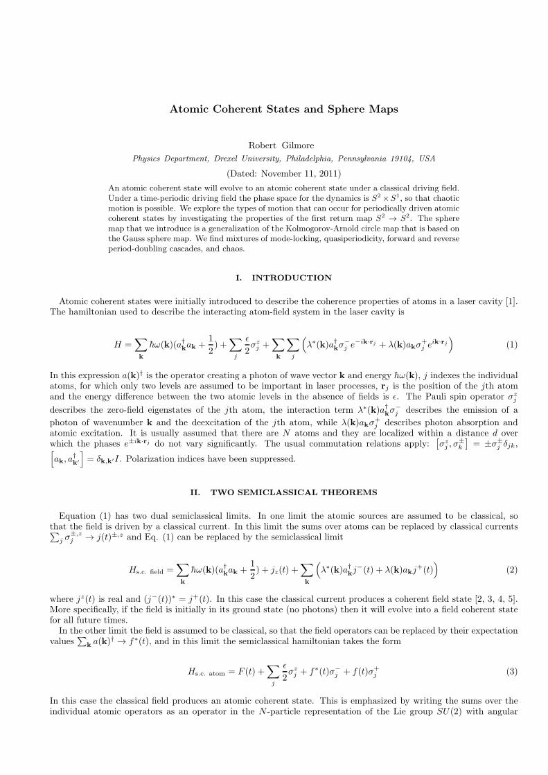
For a > 0 the circle is pushed in toward the center around θ = π. The deformation under the Gauss map is invertiblefor 0 ≤ a < 1 and noninvertible for 1 ≤ a. The curve is nonsingular for |a| < 2 and singular for 2 ≤ |a|. For |a| < 2the index is 1 and for |a| > 2 the index is 2. The gauss map θ → θ′ for the circle is shown in Fig. 2 for a = 1.5. Thismap is qualitatively similar to the Arnold circle map Eq. (7) shown in Fig. 1 for k = 1.5.A deformation of the surface of a sphere is easily represented by the spherical limacon

4

FIG. 2: The Gauss circle map is applied to the limacon r(θ) = 2 + a cos(θ), with a = 1.5. This map is qualitativelythe same as the more familiar Kolmogorov-Arnold circle map (7).

r(θ, φ) = 2− a1 sin(θ) + a2 cos(φ) (10)

It is useful to represent the Gauss sphere map (θ, φ) → (θ′, φ′) by representing the image by the point x = (φ′ − π)×sin(θ′), y = θ′. The area of the image is 4π, the area of the source.The Gauss map for the sphere surface is invertible for |a1|+ |a2| < 1 and noninvertible otherwise. For |a1|+ |a2| > 1

the mapping exhibits singularities: either two cusps or four, depending on the values of the two parameters a1 anda2. Fig. 3 shows the image of a patch of the sphere surface in the range π

2 − 34 ≤ θ ≤ π

2 + 34 and π − 3

5 ≤ φ ≤ π + 35

for a1 = 0.8, a2 = 0.7. The singularity has four cusps [14].Sphere maps of various dimensions can be constructed that involve rigid rotations and nonlinear deformations of

surfaces Sd defined by general limacons

r(θ1, θ2, . . . , θd) = 2 +d

∑

j=1

aj cos(θj) (11)

This family of maps is summarized in Table I.

V. SOME BIFURCATION SCANS

Under the map in Eq. (10) a point on the sphere will evolve, after transients have died out, to a fixed point, a modelocked orbit, a quasiperiodic trajectory, or a chaotic trajectory. Chaotic trajectories cannot occur unless the spheremap becomes noninvertible. In order to identify regions in the control parameter space ω,n, a or (ωx, ωy, ωz), (a1, a2)where interesting behavior occurs, it is useful to carry out a number of scans. The first, shown in Fig. 4, identifiesthe number of distinct points in a trajectory as a function of rotation angle ωz around the z axis as a function ofincreasing control parameters. The ratio of a1 to a2 is held fixed, and their values increase linearly from (0, 0) at thebottom of the plot to (0.8, 0.7) at the top. It is these parameter values for which the 4-cusp singularity is shown inFig. 3. Mode-locked period one orbits are indicated by a dark blue color. Mode-locked period two orbits are shown

5

FIG. 3: For 1 < |a1| + |a2| < 2 the spherical limacon Eq. (10) has a nonsingular dimple. This means the theGauss sphere map is noninvertible (1 < |a1| + |a2|) and the surface defined by Eq.(10) is nonsingular with index 1(|a1|+|a2| < 2). This plot shows how a rectangular 201×201 grid of points with π

2−34 ≤ θ ≤ π

2+34 and π− 3

5 ≤ φ ≤ π+ 35

is mapped to a singularity on the sphere surface using the spherical limacon (10) with a1 = 0.8, a2 = 0.7.

by a lighter blue color. The color coding for periodicity is shown in the color bar on the at the right. The region ofperiod-one mode locking gradually increases with increasing nonlinearity parameters. Towards the top of this figuresome chaotic behavior becomes apparent. For |a1|+ |a2| < 1 only quasiperiodicity and mode locking are possible.Fig. 5 is a scan involving rotation around the z axis. For this scan the values of the nonlinear parameters a1 and

a2 are varied according to a1 = 1.6 ∗ f, a2 = 1.4 ∗ (1− f), where f varies from 0 at the bottom of the plot to f = 1 atthe top. As f increases the singularity of the map proceeds from a double cusp in the a2 direction near f = 0, to aquadruple cusp around f = 1

2 (Fig. 3), and then back to a double cusp in the a1 direction near f = 1.A third scan is shown in Fig. 6. In this case the rotation is around the y axis and the rotation angle ωy varies from

0 to 2π along the horizontal axis. The control parameters vary according to a1 = 0.48 ∗ f and a2 = 0.42 ∗ (1 − f),with f ranging from 0 to 1. For larger values of f mostly (but not entirely) mode-locked period-one behavior is seen.Comparable scans carried out with rotations around the x axis reveal almost entirely period-one mode-locking.

TABLE I: Sphere maps are generalizations of the circle map. These maps are compositions of two maps: a rigidrotation by a rotation group operation in SO(n), and a nonlinear deformation of the sphere surface based on theGauss map of a sphere to itself. The deformation is based on a generalized limacon, given in Eq. (11). This tableprovides the number of parameters for each of the two maps and the nature of the generic singularity that can beencountered.

n Group Dim. Sphere Dim. Singularity Dim.Group Sphere Type “Sphere Map”

2 SO(2) 1 S1 1 A2 + A2 2

3 SO(3) 3 S2 2 4A3 5

4 SO(4) 6 S3 3 23A4 9

n SO(n) 1

2n(n− 1) S

n−1n− 1 2n−1

An

1

2(n+ 2)(n− 1)

6

FIG. 4: (color online) Scan of the behavior exhibited by the sphere map. Horizontal axis: rotation angle ωz aroundthe z axis, 0 ≤ ωz ≤ 2π. Vertical: strength of the nonlinearity, a1 = 0.8 ∗ f , a2 = 0.7 ∗ f 0 ≤ f ≤ 1. Colorcoding indicates the period of the trajectory. Cold colors (blues) indicate low period orbits. The hotter the color, themore distinct intersections the trajectory makes with the sphere surface. Such trajectories are either quasiperiodic orchaotic. Chaos cannot occur unless |a1|+ |a2| > 1.

VI. BIFURCATION DIAGRAMS

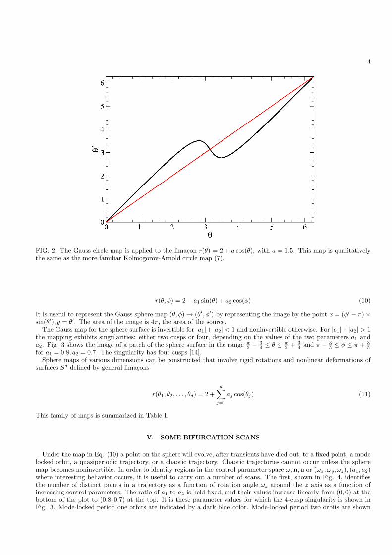
Scans of the type shown in Figs. 4, 5, and 6 give a rough indication of where to look to find interesting behavior.Bifurcation diagrams provide a way to enlarge on that information. To illustrate, we have constructed a bifurcationdiagram by taking a horizontal scan along Fig. 5 with f = 0.25. We plot (φ− π)× sin(θ) for each of several hundrediterations (after transients have died out) as a function of rotation angle ωz as the latter ranges from 0 to 2π (Fig.7). This bifurcation diagram shows an admixture of low-period mode-locking, period-bubbling [15, 16, 17, 18], andquasiperiodic behavior.Mode locking to a period-d orbit occurs at integer multiples of 2π

d radians. For example, period-one mode locking

occurs around ωz = 0, period-two around ωz = 2π2 = π radians, period-three around ωz = 2π

3 and 2 × 2π3 , and so

forth. The mode-locked regions are separated by regions with quasiperiodic orbits. The period-two and period-threemode locked regions show the begining of a period doubling “cascade” that reverses very quickly. However, otherhigher mode-locked regions show period-doubling cascades that continue to and through the accumulation point beforereversing in period-halving bifurcations. This is seen clearly in Fig. 8, which is a blowup of a small region of Fig.7. In this figure we see very clearly the mode-locked period-four and period-five regions. In the period-four regionthere is a period-doubling cascade into chaos and a reverse cascade back to period-eight (c.f., Fig. 9). The reversethen reverses to period 16, 32, ..., back into chaos, and finally reverses back all the way down to period four beforedisappearing into a quasiperiodic sea. The behavior in the period-five window is even more complex.

7

FIG. 5: (color online) Scan for which rigid rotations are about the z-axis with 0 ≤ ωz ≤ +2π (horizontal). Thedeformation parameters are a1 = 1.6∗f, a2 = 1.4∗ (1−f) with f in the range 0 ≤ f ≤ 1 (vertical). For f < 0.7 mode-locked regions are interspersed with regions supporting quasiperiodic orbits. For f > 0.7 period-doubling cascadeslead to chaotic behavior.

VII. TRAJECTORIES

The nature of a trajectory can depend sensitively on control parameter values. In order to illustrate this point wehave plotted the trajectories of the same initial condition (after transients have died out) for two slightly differentcontrol parameter values. The control parameter values are ωz = 4.64, 4.80 along the scan shown in Fig. 8. The resultsare shown in planar projection in Fig. 9. Both trajectories lie on the equator. One (ωz = 4.64) is the period-eightorbit between the pair of period-four bubbles in the period-four window that can be seen in Fig. 8. The eight pointson the trajectory are indicated by the large circles. The other (ωz = 4.80) trajectory is a quasiperiodic orbit whosecoordinates on the equator are represented by small points.

VIII. DISCUSSION AND CONCLUSION

Atomic coherent states are represented by points on the surface of a sphere S2. Under the action of a semi-classical hamiltonian Hs.c atom atomic coherent states evolve on the surface of the sphere. If the hamiltonian istime-independent the evolution is either a fixed point or a periodic orbit whose period is determined by the eigenval-ues of the semiclassical hamiltonian (difference of adjacent eigenvalues). If the semiclassical hamiltonian is periodic thephase space expands from S2 to S2×S1, the classical-like equations of motion for the point on the sphere representingthe coherent state become more difficult to integrate, and motion can be quasiperiodic or chaotic.

8

FIG. 6: (color online) Scan for which rigid rotations are about the y-axis with 0 ≤ ωy ≤ +2π (horizontal). Thedeformation parameters are a1 = 0.48 ∗ f, a2 = 0.42 ∗ (1 − f) with f in the range 0 ≤ f ≤ 1 (vertical). Mode-lockedregions are interspersed with regions supporting quasiperiodic orbits. For this deformation parameter values thesphere map is invertible and chaotic behavior cannot occur.

In order to investigate the range of possible behaviors we studied the first return map for an arbitrary periodicdrive. This is the map S2 → S2, the sphere map. There are various ways to define a sphere map [8]. In this workwe have chosen a natural generalization of the Arnold circle map. The generalization consists of the composition oftwo maps. One is “linear” in the sense that it is a rigid rotation of the sphere by the orthogonal group SO(3). Thesecond is a nonlinear deformation of the sphere surface. This deformation is constructed using the Gauss map of asurface to a sphere, where the surface is a two-parameter spherical limacon. The two parameters are related to thetwo coordinate directions on the sphere surface. Generalization of such sphere maps to higher dimensions have beensuggested. Our sphere map S2 → S2 depends on three rotation parameters and two nonlinear parameters. We haveverified that the member of the sphere map family S1 → S1 on the circle is qualitatively the same as Arnold’s circlemap. The comparison is shown in Figs. 1 and 2.The sphere map is invertible until the parameter values become large enough. When the two parameters become

large enough the map is noninvertible and chaotic behavior is in principle possible. The singularity type encounteredin the transition from invertible to noninvertible is either a double cusp or a pair of double cusps, as shown in Fig. 3.Three scans were taken to reveal roughly under what conditions the various types of behavior will exist. These are

shown in Figs. 4, 5, and 6. Further investigation of the types of behavior suggested in these plots was carried outwith bifurcation plots, as seen in Fig. 7. This figure shows harmonic mode-locked regions with basic orbits of periodn sandwiched between regions in which quasiperiodic orbits are present. Further, the mode-locked orbits of period nundergo period doubling cascades that eventually reverse back to period n. Some period “bubbling” bifurcations areclearly evident in Fig. 8. The distinction between periodic orbits and quasiperiodic orbits is clearly made in Fig. 9.We have just begun to explore the rich variety of behaviors that the sphere map S2 → S2 can exhibit.

9

FIG. 7: A bifurcation diagram is obtained by plotting the value of (φ− π)× sin(θ) against the angle of rigid rotationaround the z-axis, ωz, for a1 = 1.6 × f , a2 = 1.4 × (1 − f) and f = 0.25. This diagram shows regions of directand inverse period-doubling, quasiperiodic orbits, and chaos. Period-two (and four) orbits exist around 2π

2 , period

three orbits (and multiples) exist around 2π3 and 2 × 2π

2 , etc. Although φ varies from iteration to iteration, θ = π/2throughout this range of rotation angle values.

This work was supported in part by NSF Grant PHY 0754081.

REFERENCES

[1] F. T. Arecchi, E. Courtens, R. Gilmore, and H. Thomas, Atomic coherent states in quantum optics, Phys. Rev.A6, 2211-2237 (1972).

[2] E. Schrodinger, The continuous transition from micro- to macro-mechanics, Naturwissen. 14, 664-666 (1926).[3] R. J. Glauber, The quantum theory of optical coherence, Phys. Rev. 130, 2529-2539 (1963).[4] R. J. Glauber, Coherent and incoherent states of the electromagnetic field, Phys. Rev. 131, 2766-2788 (1963).[5] R. J. Glauber, Quantum Theory of Optical Coherence. Selected Papers and Lectures, Weiheim: Wiley-VCH, 2007.[6] E. A. Jackson, Perspectives on Nonlinear Dynamics, Cambrdige: University Press, 1989.[7] R. Gilmore and M. Lefranc, The Topology of Chaos, NY: Wiley, 2002.[8] K. Gilmore and R. Gilmore, Introduction of the sphere map with application to spin-torque nano-oscillators,

World Scientific Review (in press).[9] V. I. Arnold, Small denominators and problems of stability of motion in classical and celestial mechanics, Russian

Math. Surveys 18(6), 85-191 (1963).[10] V. I. Arnold, Small denominators. I. On the mappings of the circumference onto itself, Trans. Am. Math. Soc.

2nd Ser. 46, 213 (1965).[11] E. P. Wigner, Group Theory, NY: Academic Press, 1959.[12] R. Gilmore, Lie Groups, Lie Algebras and Some of Their Applictions, NY: Wiley, 1974.[13] D. J. Struik, Differential Geometry, Reading, MA: Addison-Wesley, 1950.[14] R. Gilmore, Catastrophe Theory for Scientists and Engineers, NY: Wiley, 1981.[15] U. Parlitz and W. Lauterborn, Resonances and torsion numbers of driven dissipative nonlinear oscillators, Z.

Naturforsch. 41a, 605-614 (1986).[16] U. Parlitz, V. Englisch, C. Scheffczyk, and W. Lauterborn, Bifurcation structure of bubble oscillators, Acoust.

Soc. Am. 88, 1061-1077 (1990).

10

FIG. 8: Blowup of Fig. 7 for the same parameter values. This clearly shows that regions of quasiperiodicity areseparated by regions of modelocking based on period 3 (to the left of 4.4), 4, 5, 6, ... . Each of the mode-lockedregions seen here proceeds through a period-doubling cascade to chaos, and then unwinds this process in a period-halving cascade back to the basic mode-locked period, before disappearing into quasiperiodic behavior.

[17] R. Gilmore and J. W. L. McCallum, Superstructure in the bifurcation diagram of the Duffng oscillator, Phys.Rev. E51, 935-956 (1995).

[18] R. Gilmore, Topological analysis of chaotic dynamical systems, Revs. Mod. Phys. 70, 1455-1530 (1998).

11

FIG. 9: Nearby control parameter values produce trajectories with distinctly different properties. A mode-lockedperiod-eight trajectory is generated with ωz = 4.64 in Fig. 8, and the quasiperiodic trajectory corresponds toωz = 4.80. The coordinates (θ, φ) defining a point on the surface S2 are mapped into the points ((φ− π)× sin(θ), θ).The boundary of this region is shown. The area enclosed is 4π. For both trajectories the value of the θ coordinate isπ2 for all points.