Atomizing Flow Simulations Using a Eulerian Multiphase Model · Atomizing Flow Simulations Using a...

Available online www.ejaet.com

European Journal of Advances in Engineering and Technology, 2017, 4 (2): 81-89

Research Article ISSN: 2394 - 658X

81

Atomizing Flow Simulations Using a Eulerian Multiphase Model

Ahmed Abounassif and Jie Cui

Department of Mechanical Engineering, Tennessee Technological University, Cookeville, TN, USA

[email protected]

_____________________________________________________________________________________________

ABSTRACT

Atomization of liquid sprays is a widely popular application utilized in increasing the efficiency of combustion ap-

plications. The number and size of liquid droplets play a crucial role in obtaining the optimal drop size distribution

for the reaction and evaporation processes within a combustion chamber. A generalized numerical model that de-

scribes the fragmentation phenomena is evaluated and applied to both two- and three-dimensional simulation mod-

els for comparison with experimental data.

An Eulerian multiphase model consisting of a continuous air phase and several discrete fuel phases is developed

and applied to a simplified 2D axisymmetric and 3D geometry in order to gain a fundamental understanding of the

differences, advantages, and limitations in the geometries. Both geometric simulations utilized the same conserva-

tion equations that required several user-defined parameters, including the breakage frequency constant and a

breakage kernel parameter. The multiphase model was simulated based on a variety of flow conditions and com-

pared with the experimental data. It can be concluded that the 2D model is capable of qualitatively predicting vari-

ous spray parameters such as total volume flux and Sauter mean diameter, while the 3D model showed good quanti-

tative agreement. The 3D model was also capable of predicting non-zero Sauter mean diameter values at the cen-

terline unlike the limited 2D axisymmetric model. The 3D model demanded greater computational power as ex-

pected, though the solution converged at a much faster rate than the 2D axisymmetric model. This is primarily due

to the sequential solution procedure required for the 2D model as it involves a greater number of control equations.

There are many factors that affect the complexity of a Eulerian multiphase flow and the current paper will facilitate

further studies as there are no guarantees to any individual simulation.

Key words: Multiphase flow, breakage kernel, discrete phase, particle distribution, CFD

_____________________________________________________________________________________

INTRODUCTION

The use of liquid sprays is very common in many industrial applications such as the propulsion of aircrafts and

rockets, burners, mixers, and other combustion processes. The liquid jet entering the combustion chamber through a

nozzle plays a significant role in the study of the surface area of the liquid, droplet size distribution, the spray angle

and other phenomena used to better understand problems involving multiphase flows. Atomization occurs as the

liquid jet is exposed to a high-velocity gas, such as air, resulting in a wide range of liquid drop sizes. The optimum

drop size distribution is desired in the combustion of fuels to achieve high rates of mixing and evaporation [1].

The present document discusses the numerical simulation of fluid particle flows using an Eulerian multiphase model

within the software package FLUENT. The model is sufficient in describing the evolution of drop sizes, air and fuel

phase behaviours, and also the particle motions at any time throughout the combustion process. The current applica-

tion of the Eulerian multiphase flow is for a simplified geometry of an aircraft engine spray combustor. Prior to

entering the combustion chamber, fuel and air are injected through their respective variable cross-section nozzles,

resulting in a rapidly expanding mixture upon reaching the exit causing catastrophic phase inversion and forming

droplets. Many complicated features can occur in such a turbulent flow field combustor, such as swirl, recirculation,

and combustion, and thus both numerical simulations and experiments are necessary. However, it is known that

certain restrictions are inevitable in standard numerical models, leading to failure in the prediction of swirling flows,

and a difference in levels of accuracy depending on the computational setup [2]. A great number of parameters af-

fect the complexity of the flow field and the resulting mass transfer and momentum. Examining such effects solely

Abounassif and Cui Euro. J. Adv. Engg. Tech., 2017, 4 (2):81-89

______________________________________________________________________________

82

by means of experimentation is extremely difficult and may cause discrepancies by different authors due to different

facilities and laboratory equipment. Therefore, a supplemental numerical approach can identify and quantify particu-

lar influences more easily.

The pertinent multiphase flow model consists of one continuous fluid phase and a set number of discrete phases,

which are capable of mass transfer with only other discrete phases while also being capable of exchanging linear

momentum with only the continuous phase [1]. Due to the complexity of the model, it is necessary to make the

proper assumptions in order to achieve a successful numerical representation. It is advantageous to utilize an Eu-

lerian multiphase model for both continuous and dispersed phases as this approach can be applied to any flow region

regardless of the local values of the volume fraction [3]. Also, as numerous size variations can occur throughout the

flow field, only one average diameter is used to characterize particle sizes within the control volume for the sake of

efficiency.

There are numerous works that study and compare numerical simulation results from FLUENT using both 2D and

3D models, whether they pertain to multiphase flow, jet spray, or any theoretical problem regarding fluid flow,

thermodynamics, heat transfer, and other scientific and engineering applications. The 2D model is a quick and effi-

cient way in producing results for a general comparison with experimental data, while 3D modelling requires more

time in computation as it adds greater depth to the problem. The 2D model can be viewed as a simple ‘slice’ of the

3D model that allows for a greater degree of freedom due to the extra dimension. The realism of the 3D model de-

mands a larger number of variables and equations to be solved, thus necessitating considerable computer power.

Aside from altering the geometry, very little needs to be done in the variation of the computational setup. Some

studies give preference to 2D modelling, while others 3D, as they are dependent on the nature of the problem as well

as the resources.

A recent study models the numerical simulation of an annular jet with a fluidic control [4]. It evaluates the flow

field sensitivity to the control jet, focusing mainly on the nozzle location in a 2D axisymmetric model rather than 3D

which significantly influenced computer time, thus enabling an increased number of solved geometry variants.

However, no asymmetrical effects can be simulated with such a simplified model. Another recent study similarly

favours 2D axisymmetric modelling of a gas atomization nozzle for gas flow behaviour for the same reasons as only

half of the axial section of the atomizer is required [5]. The study also emphasizes grid refinement to the necessary

level in order to capture the desired results while keeping in mind the obligatory increase in computational time.

There has also been an investigation on CFD modelling of three-phase flow hydrodynamics in a jet-loop reactor

which used an Eulerian-Eulerian model approach to predict flow behaviour [6]. The authors chose a 2D axisymmet-

ric solver knowing that a 3D model would provide extensive knowledge about bubble rising and flow hydrodynam-

ics, but would be unsuitable for such industrial scale reactors. Such a 2D model may have shortened computational

time; however significant errors in the vicinity of the axis of symmetry had occurred, which were ultimately reduced

to acceptable values when an unstructured grid mesh was used.

A master’s thesis describes the importance in utilizing predictive tools for turbulent reacting flows, with a portion of

paper describing comparisons with a 2D and 3D simulation of air injection through specific nozzle geometry [2].

The paper stresses that axial and swirl velocities for the 2D simulation agree well with experimental data near the

inlet, unlike farther downstream where the prediction accuracy decreases. Grid refinement for the 2D case did noth-

ing to improve the solution and instead introduced convergence problems and reversed flow on the outlet. With the

3D simulation, not only did the solution converge faster, but great improvements were clear farther downstream,

probably due to the anisotropic effects as they are more carefully taken into account by the model.

In summary, many previous studies, both related and independent to multiphase jet flow, conveyed the differences

in 2D and 3D models to be minimal in some cases, while the latter requires immense computational power and re-

sources. Incidentally, 3D models are capable of simulating behaviour that is non-existent in the 2D, while 2D re-

quires careful setup to achieve results with greater accuracy. Grid refinement must also be studied as it may further

enhance the results or on the other hand prove costly with regards to computational time. While 3D models seem to

provide greater accuracy in most cases due to the more realistic features, the most suitable model will vary depend-

ing on the nature of the problem, the intricacy of the geometry, and the available time and resources. Results can be

considered reliable with proper experimental validation.

The objective of this study is to simulate 2D and 3D multiphase flow models using FLUENT in order to observe the

differences between the models and see how well they compare with experimental data. The design of many geo-

metrical and parametric variants, their manufacturing and experimentation require time, extreme caution, and con-

siderable expenses. Therefore, with the recent advances in computational power, the application of computational

fluid dynamics (CFD) is considered the basis in creating reasonable and meaningful comparisons in numerical simu-


______________________________________________________________________________

83

lation provided careful consideration is taken into account. For the particular flow presented in this paper, both 2D

and 3D simulations will be performed under various flow conditions for which the results will be compared. Many

factors including flow velocity and grid size will be varied in order to study the sensitivity or lack thereof which

may facilitate further studies of this flow model as there will be no guarantees to the outcome of any individual sim-

ulation.

GOVERNING EQUATIONS

FLUENT can solve mass and momentum conservation equations for all types of flows in 2D axisymmetric and 3D

geometries. Both geometric models utilize the same mass and linear momentum conservation equations pertaining

to axial, radial, and swirl velocities, as well as external body forces that arise from the interaction of the continuous

phase with the dispersed phase.

There are three types of Euler-Euler multiphase models available, but this paper will only focus on the Eulerian

multiphase model, solving a set of momentum and continuity equations for each phase. The model will include a

continuous phase and several discrete particle sizes of a fluid phase. The continuous phase will be assigned as air

and designated a phase number 0. The remaining discrete particles will be designated as 1, 2, 3…M and will be

given a particular phase diameter as assigned from the user-defined function. In Eulerian multiphase models,

balance laws for mass and linear momentum are solved separately for each individual phase with the phases being

allowed to interact through source terms [1].

FLUENT was used to solve all the equations which are presented from their manual [7]. The conservation of mass

for the continuous phase (i=0) can be written as 𝜕

𝜕𝑡(𝛼0𝜌0) + ∇. (𝛼0𝜌0�⃗�0) = 0 (1)

where 𝛼0 is the volume fraction, 𝜌0 is the density, �⃗�0 is the velocity field. The balance of linear momentum for this

phase yields 𝜕

𝜕𝑡(𝛼0𝜌0�⃗�0) + ∇. (𝛼0𝜌0�⃗�0�⃗�0) = −𝛼0∇𝑝 + ∇. �̿�0 − ∑ 𝐾0𝑖(�⃗�0 − �⃗�𝑖)𝑀

𝑖=1 (2)

where �̿�0 is the extra stress tensor of phase 0, p represents a common hydrodynamic pressure field shared by all

phases and K0i is the interphase momentum exchange coefficient. Using the source terms to generate mass and mo-

mentum exchange between the discrete phases (i=1...M), the balance of mass and linear momentum can be written

in the form presented below. 𝜕

𝜕𝑡(𝛼𝑖𝜌𝑖) + ∇. (𝛼𝑖𝜌𝑖�⃗�𝑖) = −𝜌𝑖𝛤𝑖𝛼𝑖 + 𝜌𝑖 ∑ 𝑛𝑖𝑗𝑥𝑖

(𝑖−1)𝑗=1 𝛤𝑗

𝛼𝑗

𝑥𝑗 (3)

𝜕

𝜕𝑡(𝛼𝑖𝜌𝑖�⃗�𝑖) + ∇. (𝛼𝑖𝜌𝑖�⃗�𝑖�⃗�𝑖) = −𝛼𝑖∇𝑝 + ∇. �̿�𝑖 + 𝐾0𝑖(�⃗�0 − �⃗�𝑖) − 𝜌𝑖𝛤𝑖𝛼𝑖�⃗�𝑖 + 𝜌𝑖 ∑ 𝑛𝑖𝑗

(𝑖−1)𝑗=1 𝑥𝑖𝛤𝑗

𝛼𝑗

𝑥𝑗�⃗�𝑗 (4)

Here αi represents the volume fraction, ρi the density, and �⃗�𝑖 the velocity field for the ith drop phase. Γi is the break-

age frequency of particles of size xj, and nij is the number of daughter drops of size xi formed from a parent drop of

size xj. The breakage frequency function employed in the present work is of the form

𝛤𝑖 = 𝛤0(𝑑𝑖 − 𝑑𝑀)|�⃗�0 − �⃗�𝑖|2 (5)

where Γ0 is a breakage frequency constant and di is the particle diameter associated with the ith size class. The

breakage frequency function is correlated to the relative motion between phases and drop phase surface tension to

cause fragmentation to cease at an axial distance further away from the nozzle. The last two terms in Equation (4)

represent, respectively, the death and birth terms associated with phase i [1].

The nij coefficient from Equations (3) and (4) can be calculated using the breakage kernel β(xi,xj) of the continuous

population balance model by the equation

𝑛𝑖𝑗 = ∫(𝑥𝑖+1−𝑉)

(𝑥𝑖+1−𝑥𝑖)

𝑥𝑖+1

𝑥𝑖𝛽(𝑉, 𝑥𝑗)𝑑𝑉 + ∫

(𝑥𝑖−1−𝑉)

(𝑥𝑖−1−𝑥𝑖)

𝑥𝑖

𝑥𝑖−1𝛽(𝑉, 𝑥𝑗)𝑑𝑉 (6)

as presented by Kumar and Ramakrishna [8]. For all the results discussed in this paper, the nij values are calculated

using Equation (6) from the breakage kernel

𝛽(𝑥𝑖 , 𝑥𝑗) = 𝑐 (12

𝑥𝑗[

𝑥𝑖

𝑥𝑗− (

𝑥𝑖

𝑥𝑗)

2

]) + (1 − 𝑐) (24

𝑥𝑗[

𝑥𝑖

𝑥𝑗−

1

2]

2

) (7)

where a range of realistic breakage kernel forms can be obtained by varying the parameter c between 0 and 1. Sev-

eral noteworthy kernels are obtained by setting c = 1, 0, and 2/3 for equisized, erosion, and equal fragments, respec-

tively. The equisized kernel refers to the phenomenology when the formation of equal-sized daughter drops is en-

couraged, while the erosion kernel refers to the formation of daughter particles of vastly different sizes. Initially,

only the equal fragments kernel is considered which will allow all daughter size classes to receive an equal number

of particles.


______________________________________________________________________________

84

GEOMETRIC MODEL

The geometrical model in both 2D and 3D was generated using the GAMBIT software and then exported into FLU-

ENT to simulate the aforementioned multiphase flow. A detailed 3D geometrical model was provided by the

Goodrich Corporation from which the dimensions were extracted in order to create the simple yet sufficient 2D

model of the nozzle geometry. After it was meshed and exported into FLUENT, the 2D model was upgraded into a

3D model using the methodology described in this section.

Only the upper half of the 3D model provided by Goodrich had been used to create the 2D model due to its axisym-

metric nature. Figure 1 shows an overall result of creating the 2D model. A series of vertex points had been gener-

ated using the x and y coordinates given in the 3D detailed model. The vertex points were then connected to each

other by edges which are then unified in order to create what is called a ‘face’ in GAMBIT. Boundary zones need to

be specified once the face is created, and Figure 1 shows the locations of the pressure outlets, and the axis of sym-

metry. Figure 2 indicates the inlet region and the nozzle locations of the inner air, fuel, and outer air, while all other

edges are specified as ‘wall.’ There are a variety of techniques in creating a meshed grid for this model, but the cur-

rent study will only focus on using a size function, in which an initial cell size, growth rate, and maximum size are

required by GAMBIT. This technique enables the user to refine only the necessary region of the mesh, in this case

being near the inlet region, while transitioning smoothly into a relatively coarse mesh at the downstream region to

save computational time.

The 3D model requires only a few modifications to the 2D model, but these can only be made after removing the

mesh as well as the axis symmetry. The remaining edges were revolved about the x-axis at a 360-degree angle, cre-

ating multiple faces. A 3D volume is then generated as a result of ‘stitching’ the faces together in GAMBIT. Once

the volume is created, the boundary zones will need to be specified again as they are considered ‘faces’ in 3D as

oppose to ‘edges’ in the 2D model. Also, a new size function is necessary in meshing the volume as shown in Fig-

ures 3 and 4. In order to study and compare results between the 2D and 3D models, it is imperative to create a

cross-sectional surface on the ‘z’ plane of the 3D model for a better understanding of the results.

Both the 2D and 3D models utilize the same numerical methodology in FLUENT except that the 2D version needs

to be specified as an axisymmetric model. All the equations used in solving the models are also the same except for

the axisymmetric swirl equations included in the 2D model. The current section will describe the general solution

procedure for the models.

Fig.1 2D Model with 22,524 cells Fig.2Nozzle Region of 2D Model

Fig.3 3D model with 294,271 cells Fig.4 Nozzle Region of the 3D Model


______________________________________________________________________________

85

Once the model is meshed, it needs to be exported as a mesh file in order for FLUENT to recognize it. A few sim-

ple yet crucial steps need to be taken care of first, such as specifying the units used in creating the geometry, and

identifying the multiphase model as Eulerian and the viscous model as standard k-ε. The number of phases also

needs to be specified, with 10 discrete fuel phases, and 1 continuous air phase based on the user-defined function

(UDF) created by Rayapati [1]. The fuel used in this study will have unique physical properties provided by

Goodrich and will need to be created manually as a new material. Furthermore, all the inlet velocities, turbulent

kinetic energies, turbulent dissipation rates, and initial phase volume fractions need to be input accordingly.

Prior to beginning the solution process, the UDF must be compiled and loaded into FLUENT. The UDF consists of

various sub-functions some of which are executed for every iteration and some are executed at the loading step in

the solution process. The EXECUTE_ON_LOADING sub-function executes during loading by calculating the di-

ameters of each particle size, the coefficients nij, and flow independent breakage frequencies associated with each

particle size. The remaining sub-functions are executed at the top of the iteration during the solution process. Any

flow dependent parameters, such as relative velocity or local Weber numbers, can be calculated in the DE-

FINE_ADJUST sub-function and can be stored in a user-define memory location for later use in other sub-functions.

Finally, the mass and momentum source terms resulting from the fragmentation phenomenon are added to the asso-

ciated balance equation by the DEFINE_SOURCE sub-function.

A sequential solution procedure may be required for obtaining the convergent solution for an axisymmetric swirl

multiphase problem since the presence of high swirl velocities enhances the complexity in solving the conservation

equations. Such high swirl velocities create a large radial pressure gradient which in turn determines the distribution

of swirl in the flow field. Due to this higher degree of coupling, instability may be inevitable and thus a special so-

lution strategy is necessary. In the ‘Solutions Control’ panel, the flow and turbulence equations need to be comput-

ed for only the primary phase by deselecting the volume fraction and swirl equations. Then the swirl equation must

be activated to calculate the complete solution for a single phase problem, and then deactivated again after obtaining

an intermediate solution. The multiphase problem can then be solved by enabling only the flow, turbulence and

volume fraction equations. Finally, all equations must be selected to solve the complete multiphase problem with

induced swirl. If the convergence problem still persists, then it is recommended to start the calculation with a small

swirl velocity and to increase it gradually until the desired value is reached [1].

MODEL RESULTS AND COMPARISONS

In this section, the results of the 2D axisymmetric model and 3D model simulations are discussed. Grid refinement

was a crucial step in the simulations in order to save computational time while retaining adequate resolutions.

All the results presented are at a radial location that ranges from 0 – 80 mm at various axial locations. The results

include total fuel volume flux and the fuel Sauter Mean Diameter (SMD), which is defined as the diameter of a drop

having the same volume to surface area ratio as the entire spray. The total fuel volume flux can be calculated by

𝑉𝑓𝑙𝑢𝑥 = ∑ 𝑣𝑥𝑖𝛼𝑖

𝑀𝑖=1 (8)

where vxi is the axial velocity for the ith fuel phase. Also the Sauter Mean Diameter

𝑠𝑚𝑑 =∑ 𝛼𝑖

𝑀𝑖=1

∑𝛼𝑖𝑑𝑖

𝑀𝑖=1

(9)

where di is the droplet diameter for fuel phase i. The volume flux presents the fuel distribution across the spray en-

velope, which is of critical importance in many industrial applications. Many applications require arrays of nozzles

in order to effectively cover large areas and so optimization of the atomizer depends upon accurate spray volume

flux measurements. Precise measurement of the spray distribution is also necessary to determine appropriate sam-

pling protocols for drop size and velocity measurements.

The fuel SMD is extensively used in the characterization of liquid/liquid or gas/liquid dispersions primarily due to

the relation of the area of the dispersed phase to its volume and hence to mass transfer and chemical reaction rates

[9]. It is particularly important in liquid spray combustion of a fuel, as this occurs only at the interface between a

droplet’s surface and the surrounding oxygen. As a result, the fuel burns best when the drop surface area is maxim-

ized and the internal drop volume is minimized. Therefore, a small Sauter mean diameter infers better combustion

efficiency due to a larger surface area in relation to the volume or amount of fuel being burned. However, it must be

borne in mind that SMD is influenced by properties of the atomizing fluids as well as by the nozzle design and the

operating conditions. SMD also expresses the fineness of a spray which plays an important factor in the nozzle per-

formance. For gas absorption and chemical injection, the surface area of the droplet controls the rate and extent of

the reaction, and must be optimized for the given process. In gas cooling applications, the droplet size is critical as

it must be small enough in order for complete evaporation to occur at a faster rate.


______________________________________________________________________________

86

0

20

40

60

80

100

120

140

160

180

200

0 20 40 60 80

SMD

(m

icro

ns)

Radial Position (mm)

Experimental2D CFD at 13 mm3D CFD at 13 mm2D CFD at 25 mm3D CFD at 25 mm

0

20

40

60

80

100

120

0 20 40 60 80

SMD

(m

icro

ns)


Experimental

2D CFD at 13 mm

3D CFD at 13 mm

2D CFD at 25 mm

3D CFD at 25 mm

0

0.02

0.04

0.06

0.08

0.1

0.12

0.14

0 20 40 60 80

Vfl

ux

(cc/

cm2 /

sec)


Experimental

2D CFD at 25 mm

3D CFD at 25 mm

2D CFD at 50 mm

3D CFD at 50 mm

0

0.05

0.1

0.15

0.2

0.25

0.3

0 20 40 60 80

Vfl

ux

(cc/

cm2 /

sec)


Experimental

2D CFD at 25 mm

3D CFD at 25 mm

2D CFD at 50 mm

3D CFD at 50 mm

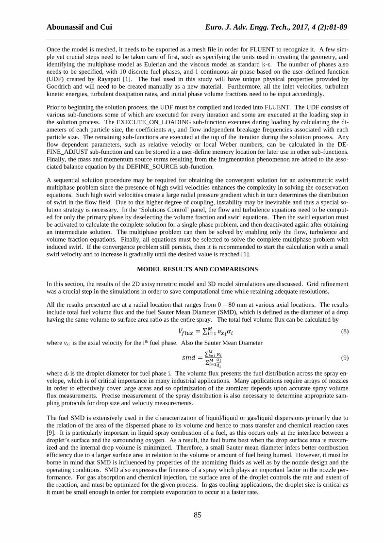
The following sets of figures show experimental results generated from the Goodrich Corporation using a Phase

Doppler Particle Analyser (PDPA) and will be compared with the CFD results. It is common in dense sprays that

the performance of such a device will be poor and subject to significant error, however modifications have been

recently proposed to improve measurement accuracy. The main deficiency of the current state of the art in experi-

mental diagnostics of particulate systems is that they are unable to explicitly conserve mass during the measurement

process [10].

All the experimental data is given at 25 mm axial distance, with the CFD provided at 25 mm as well as 13 mm and

50 mm depending on the figure. Although the 3D results demanded greater computational power, the solutions con-

verged at a much faster rate as only a few thousand iterations were required compared to the 100,000+ for the 2D

model. Also, the 3D solution procedure only required three control equations, all of which can be selected from the

start with no risk of instability.

Figures 5 – 8 present several of the experimental and CFD comparisons in the same graph for a clearer overview.

For the figures involving Sauter mean diameter, the 3D CFD results agree better than the 2D CFD in a quantitative

sense, however the opposite is true qualitatively. The experimental data follow a similar pattern to 2D; however, the

3D simulations generated non-zero SMD values at the centreline and with good agreement, especially for the low

flow conditions as shown in Figure 6. And for both 2D and 3D results, the axial location of 13 mm seems to agree

better than those at 25 mm. For the figures involving volume flux, both 2D and 3D results show similar agreement

at an axial distance of 50 mm, and similar disagreement at 25 mm. Similar observations can be made for all cases in

this study.

Fig.5 Comparing SMD at High Flow Fig.6 Comparing SMD at Low Flow

Fig.7 Comparing Total Volume Flux at High Flow Fig.8 Comparing Total Volume Flux at Low Flow

PARAMETRIC STUDY

There are two crucial elements in characterizing the fragmentation of the population balance model. One is the

daughter-size distribution kernel which describes the number of particles and the particle size distribution produced

by a single event. The second is the breakage frequency which describes the rate at which the particles break up per

unit time. Both elements provide a complete description of the birth and death events associated with each member

of the continuous particle size distribution, and can therefore be used as the basis of discretization.


______________________________________________________________________________

87

0

20

40

60

80

100

120

140

160

180

200

0 20 40 60 80

SMD

(m

icro

ns)


Experimental2D CFD at 13 mm c=2/32D CFD at 13 mm c=02D CFD at 13 mm c=12D CFD at 25 mm c=2/32D CFD at 25 mm c=02D CFD at 25 mm c=1

0

20

40

60

80

100

120

140

160

180

200

0 20 40 60 80

SMD

(m

icro

ns)


Experimental3D CFD at 13 mm c=2/33D CFD at 13 mm c=03D CFD at 13 mm c=13D CFD at 25 mm c=2/33D CFD at 25 mm c=03D CFD at 25 mm c=1

0

0.02

0.04

0.06

0.08

0.1

0.12

0 20 40 60 80

Vfl

ux

(cc/

cm2 /

sec)


Experimental

2D CFD at 25 mm c=2/3

2D CFD at 25 mm c=0

2D CFD at 25 mm c=1


2D CFD at 50 mm c=0

2D CFD at 50 mm c=1

0

0.02

0.04

0.06

0.08

0.1

0.12

0.14

0 20 40 60 80

Vfl

ux

(cc/

cm2 /

sec)


Experimental


3D CFD at 25 mm c=0

3D CFD at 25 mm c=1


3D CFD at 50 mm c=0

3D CFD at 50 mm c=1

0

20

40

60

80

100

120

140

160

180

200

0 20 40 60 80

SMD

(m

icro

ns)


Experimental3D CFD at 13 mm 8k3D CFD at 13 mm 4k3D CFD at 13 mm 16k3D CFD at 25 mm 8k3D CFD at 25 mm 4k3D CFD at 25 mm 16k

0

50

100

150

200

250

300

0 20 40 60 80

SMD

(m

icro

ns)



Figures 9 – 12 display the effects of different breakage kernel forms by varying the parameter ‘c’ for an erosion

kernel (c=0) and equisized kernel (c=1). It can be observed that varying ‘c’ does not instigate a major change in the

results, however there is a greater effect in SMD and volume flux for the erosion kernel as compared to the

equisized kernel. This can be due to the nature of the erosion kernel with which the probability of obtaining vastly

different daughter particle sizes in a single breakage event is high.

Fig.9 Varying the Breakage Kernel paramenter ‘c’ – 2D SMD Fig.10 Varying the Breakage Kernel paramenter ‘c’ – 3D SMD

Fig.11 Varying the Breakage Kernel paramenter ‘c’ – Fig.12 Varying the Breakage Kernel paramenter ‘c’ –

2D Total Volume Flux 3D Total Volume Flux

Fig.13 Varying the Breakage Frequency ‘gamma’ – 2D SMD Fig.14 Varying the Breakage Frequency ‘gamma’ – 3D SMD


______________________________________________________________________________

88

0

0.02

0.04

0.06

0.08

0.1

0.12

0.14

0 20 40 60 80

Vfl

ux

(cc/

cm2 /

sec)



0

0.02

0.04

0.06

0.08

0.1

0.12

0.14

0.16

0.18

0 20 40 60 80

Vfl

ux

(cc/

cm2/s

ec)



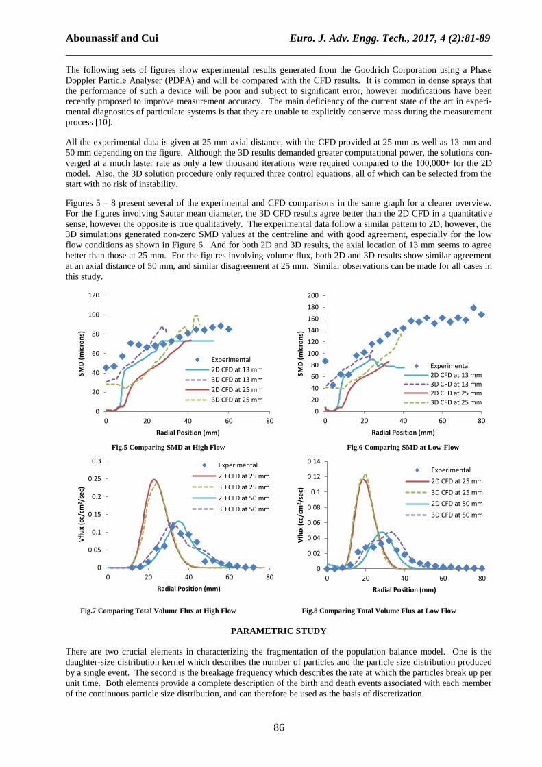
Fig.15 Varying the Breakage Frequency ‘gamma’ Fig.16 Varying the Breakage Frequency ‘gamma’

2D Total Volume Flux 3D Total Volume Flux

Figures 13 – 16 show the effects of halving and doubling the breakage frequency ‘gamma’ originally set at 8000 s-1.

It can be observed that halving the frequency greatly increases the SMD and has the opposite effect for doubling the

value. Similarly halving the frequency decreases the volume flux, while the opposite occurs for doubling the value

and to a greater effect for the 3D model. These results can be explained by the fact that less breakage indicates

larger particle sizes, which tend to be transported radially farther than that of a smaller class size as shown in Figure

16. Such effects can be due to the combination of the drag force and radial velocity induced by the swirling flow.

CONCLUSION

In this paper, the development of an Eulerian multiphase model for comparing the drop size distribution and

fragmentation in both a 2D axisymmetric and a 3D model is discussed. The aforementioned Eulerian multiphase

model incorporates air as the continuous phase plus ten discrete fuel phases, with each discrete phase representing a

particle size class with its own velocity field. The mass transfer was calculated using the discrete population balance

approach which was applied to FLUENT using user-defined mass and momentum source terms in the respective

balance equations.

Numerical simulations were performed on different grid sizes for both 2D and 3D models to establish grid

independence. Symmetry was also confirmed with the 3D model. The models were simulated under various

different flow conditions where experimental data was available and results compared. Although the 3D model

demanded greater computational power, the solution process was simpler and convergence was achieved at a much

faster rate than for the 2D axisymmetric model.

The 2D CFD model showed an overall qualitative agreement with the experimental data, while the 3D model more

quantitative. Also, the 3D model was capable of predicting non-zero SMD values at the centerline unlike the 2D

axisymmetric model which may have been too restrictive in allowing mass to be transported towards the axis. All

the experimental data was provided at an axial location of 25 mm, however both models generated results with

better agreement at different locations, especially those for volume flux at a location of 50 mm. This may be due to

the fact that most current PDPA systems are subject to error as they are unable to explicitly conserve mass during

the measurement process. Also, the number of drops sampled from the experimental data is quite low in many of

the cases, further increasing the margin of error. After varying the breakage kernel forms, it can be concluded that

the erosion kernel impacts both models to a greater effect than the equisized kernel. Also, the outcome of the

breakage frequency variations is more significant with the 3D model results.

The 3D model generates a more realistic simulation of the multiphase flow with a depth perception that is

unattainable with the 2D axisymmetric model. Both models generated good comparable results with the

experimental data and can be utilized for any multiphase flow problem depending on the computational resources.

As a result of the simplicity of the geometry, number of phases used, and available resources, the conclusion can be

drawn that the 3D model is the more preferable choice in simulating the current atomizing flow.

Acknowledgements

Acknowledgements to the Center of Energy Systems Research of Tennessee Technological University for their fi-

nancial support.


______________________________________________________________________________

89

REFERENCES

[1] NP Rayapati, Eulerian Multiphase Model of Fragmenting Flows, Tennessee Technological University, USA,

2010.

[2] M Persson, Predictive Tools for Turbulent Reacting Flows, Lulea University of Technology, Sweden, 2001.

[3] K Pougatch, M Salcudean, E Chan, and B Knapper, A Two-Fluid Model of Gas-Assisted Atomization including

Flow through the Nozzle, Phase Inversion, and Spray Dispersion, International Journal of Multiphase Flow, 2009,

35 (7), 661-675.

[4] J Hosek, Z Travnicek, and K Peszynski, Numerical Simulation of an Annular Jet with a Fluidic Control, Devel-

opment in Machinery Design and Control, Bydgosz-Duszniki, Poland, 2002.

[5] O Aydin, and R Unal, Experimental and Numerical Modeling of the Gas Atomization Nozzle for Gas Flow Be-

havior, Computers and Fluids, 2011, 42 (1), 37-43.

[6] RG Szafran, and A Kmiec, Application of CFD Modelling Technique in Engineering Calculations of Three-

Phase Flow Hydrodynamics in a Jet-Loop Reactor, International Journal of Chemical Reactor Engineering, 2004, 2

(1), Article A30.

[7] FLUENT 12 User’s Guide, Fluent Inc, New Hampshire, 2007.

[8] S Kumar and D Ramakrishna, On the Solution of Population Balance Equations by Discretization-I. A Fixed

Pivot Technique, Chemical Engineering Science, 1996, 51 (8), 1311-1332.

[9] AW Pacek, CC Man and AW Nienow, On the Sauter Mean Diameter and Size Distributions in Turbulent Liq-

uid/Liquid Dispersions in a Stirred Vessel, Chemical Engineering Science, 1998, 53 (11), 2005-2011.

[10] JF Widmann, C Presser and SD Leigh, Improving Phase Doppler Volume Flux Measurements in Low Data

Rate Applications, Measurement Science and Technology, 2001, 12 (8), 1180 – 1190.

Date post:	27-Mar-2020
Category:	Documents
Upload:	others
View:	18 times
Download:	0 times

Atomizing Flow Simulations Using a Eulerian Multiphase Model · Atomizing Flow Simulations Using a...

Documents