1

ATTACHMENT 3

CLIMATE CHANGE AND SEA-LEVEL RISE EFFECTS FOR THE

HSC ECIP FEASIBILITY STUDY

October 2019

2

3.1 Climate Change in Coastal Texas The specific aspect of climate change that is sea level is a complex subject addressed separately in the H&H Attachment (Relative Sea Level Rise) to the H&H Engineering Appendix. This section discusses other future climate changes (mainly precipitation) based on current scientific evidence and studies. Climate change is expected to pose several challenges along the Texas coast. It is expected to vary greatly along the extensive Texas coast from the Mexican border to the Louisiana border. These challenges will unfold against a backdrop that includes a growing urban population, incentives for energy production, and advances in technology. For the current study area, the primary climatic forces with potential to affect the project are changes in temperature, sea and inland water levels, precipitation, storminess, ocean acidity, and ocean circulation. Air temperatures in the Houston-Galveston mean statistical area, on average, increased about 1 degree Centigrade over the past 20 years, a pattern that is expected to continue. Sea surface temperatures have risen and are expected to rise at a faster rate over the next few decades. Global average sea level is rising and has been doing so for more than 100 years. Greater rates of sea-level rise are expected in the future (Parris 2012). Higher sea levels cause more coastal erosion, changes in sediment transport and tidal flows, more frequent flooding from higher storm surges, and saltwater intrusion into aquifers and estuaries. Patterns of precipitation change are affecting coastal areas in complex ways. The Texas coast saw a 10 to 15 percent increase in annual precipitation between 1991 and 2012 compared to the 1901-1960 average, Figure 1. Texas coastal areas are predicted to experience heavier runoff from inland areas, with the already observed trend toward more intense rainfall events continuing to increase the risk of extreme runoff, flooding, and possibly creating safety issues.

Figure 1: Percent Change in Annual Precipitation for 1991-2012 Compared to 1901-1960 (adapted from Peterson et al. 2013)

3

Texas’ Gulf Coast historically averages three tropical storms or hurricanes every four years (annual probability of 75%), generating coastal storm surges and sometimes bringing heavy rainfall and damaging winds hundreds of miles inland. The estimated rise in sea level will result in an effective increase in storm surge along the Texas Gulf coast and miles inland. Tropical storms have increased in intensity in the last few decades. Future projections suggest increases in hurricane rainfall and intensity (with a greater number of the strongest - Category 4 and 5 - hurricanes) (Melillo 2014). As the concentration of carbon dioxide in the atmosphere increases, the oceans will continue to absorb CO2, resulting in increased ocean acidification. This threatens coral reefs and shellfish (Hoegh-Guldberg 2007). Coastal fisheries are also affected by rising water temperatures and climate-related changes in oceanic circulation. Wetlands and other coastal habitats are threatened by sea-level change, especially in areas of limited sediment supply or where barriers prevent onshore migration. The combined effects of saltwater intrusion, reduced precipitation, and increased evapotranspiration will elevate soil salinities and lead to an increase in salt-tolerant vegetation (Craft 2009). For additional information, reference the Environmental section of the FIFR-EIS. None of these changes operate in isolation. The combined effects of climate changes with other human-induced stresses make predicting the effects of climate change on coastal systems challenging. However, it is certain that these factors will create increasing hazards to the Texas coast. Heavily industrialized cities and ports containing critical infrastructure along the Texas coast, including Freeport, Port Arthur, Galveston, Corpus Christi, Matagorda, Brazos Island Harbor, Houston, Port Orange, and additional areas will be adversely affected by climate change. The projected change in sea level will result in the potential for greater damage from storm surge along the Texas coast. About a third of the GDP for the state of Texas is generated in coastal counties. Coastal areas in Alabama, Mississippi, Louisiana, and Texas already face losses that annually average $14 billion from hurricane winds, land subsidence, and sea-level change. According to a recent study, projected sea-level change increases average annual losses from hurricanes and other coastal storms (Building 2010). Diminishing water supplies and rapid population growth are critical issues in Texas. Along the coast, climate change-related saltwater intrusion into aquifers and estuaries poses a serious risk to local populations. In 2011, many locations in Texas experienced more than 100 days over 100°F, as the state set high temperature records. Rates of water loss were double the long-term average, depleting water resources. This contributed to more than $10 billion in direct losses to agriculture alone (Melillo 2014). Typically, many of the water shortages occur in the drier west parts of Texas. The agricultural economy along the Texas coast, including livestock, rice, cotton, and citrus cultivation, is threatened by the combination of salt or brackish water from sea-level change and reduced freshwater levels from changes in temperature and precipitation. Coastal ecosystems are particularly vulnerable to climate change because many have already been dramatically altered by human interventions creating additional stresses. Climate change will result in further reduction or loss of functions these ecosystems provide. Successful adaptation of human and natural systems to climate change will require commitment to addressing these challenges. Regional-scale planning and local-to-regional implementation will prove beneficial. Finding a way to mainstream climate planning into existing processes will save

4

time and money. It is important that information be continually shared among decision-makers to facilitate the alignment of goals.

Figure 2: Change in 30-year mean annual precipitation, measured in centimeters per year (cm/year). The median difference between 1971–2000 and 2041–2070 is based on 112 projections obtained from “Statistically Downscaled WCRP CMIP3 Climate Projections” (http://gdo-dcp.ucllnl.org/downscaled_cmip3_projections).

5

Figure 3: Global mean sea level (GMSL) observed since 1870 and projected for the future (deviation from the 1980–1999 mean). [For illustrative purposes only, from U.S. Army Corps of Engineers (2008); Intergovernmental Panel on Climate Change (2007, FAQ 5.1, fig. 1).] References IPCC 2007 Intergovernmental Panel on Climate Change (2007) Climate Change 2007: The Physical Science Basis. Contribution of Working Group I to the Fourth Assessment Report of the Intergovernmental Panel on Climate Change (S. Solomon, D. Qin, M. Manning, Z. Chen, M. Marquis, K.B. Averyt, M. Tignor, and H. L. Miller, ed.). Cambridge, UK: Cambridge University Press. http://ipcc-wg1.ucar.edu/wg1/wg1-report.html Melillo, Jerry M., Terese (T.C.) Richmond, and Gary W. Yohe, Eds., (2014): Climate Change Impacts in the United States: The Third National Climate Assessment. U.S. Global Change Research Program, 841 pp. doi:10.7930/J0Z31WJ2. Parris et al. 2012 Parris, A., P. Bromirski, V. Burkett, D. Cayan, M. Culver, J. Hall, R. Horton, K. Knuuti, R. Moss, J. Obeysekera, A. Sallenger, and J. Weiss (2012) Global Sea Level Rise Scenarios for the U.S. National Climate Assessment. NOAA Technical Report OAR CPO-1. Washington, DC: National Oceanic and Atmospheric Administration, Climate Program Office. http://cpo.noaa.gov/Home/AllNews/TabId/315/ArtMID/668/ArticleID/80/Global-Sea-Level- Rise-Scenarios-for-the-United-States-National-Climate-Assessment.aspx

6

USACE 2013 U.S. Army Corps of Engineers (2013) Coastal Risk Reduction and Resilience. CWTS 2013-3. Washington, DC: Directorate of Civil Works, U.S. Army Corps of Engineers. Peterson et al. 2013 Peterson, T.C., R. Heim, R. Hirsch, D. Kaiser, H. Brooks, N. Diffenbaugh, R. Dole, J. Giovannettone, K. Guirguis, T. Karl, R. Katz, K. Kunkel, D. Lettenmaier, G. McCabe, C. Paciorek, K. Ryberg, S. Schubert, V. Silva, B. Stewart, A. Vecchia, G. Villarini, R. Vose, J. Walsh, M. Wehner, D. Wolock, K. Wolter, C. Woodhouse, D. Wuebbles (2013) Monitoring and Understanding Changes in Heat Waves, Cold Waves, Floods, and Droughts in the United States: State of Knowledge. Bulletin of the American Meteorological Society, Volume 94, 821-834 pp. doi: 10.1175/BAMS-D-12-00066.1 3.2 Sea Level Rise

Report on Sea-Level Rise Effects

on the Houston Ship Channel’s Deepening and Widening Project

General guidance by Galveston District’s Hydrology and Hydraulics Branch

ABSTRACT

This report summarizes guidance for incorporating sea-level rise (SLR) into a navigation project. Specific SLR projections have been included for Houston Ship Channel. “Present Condition” sea levels for the Bay relative to Local Mean Sea Level (LMSL) are 0.44 ft in 2013 (the end year for USACE sea-level analysis), 0.52 ft in 2017 (the year of economic modeling for this project), and 0.65 ft in 2023 (the anticipated project construction year). (Levels are relative to 1992 Zero.) Projected sea-level rise has been computed for project durations of 25-year, 50-year, and 100-year timeframes. As a conservative approach, USACE’s Low Sea-Level Curve should be used for this navigation project (since it provides deeper water and less dredging than other curves). When considering channel depths (for dredging computations), both sea-level rise and subsidence are relevant. (Subsidence is more than twice the sea-level rise rate.) Under this scenario the 50-year design life channel depth will increase an additional 1.70 feet above the 2023 level. The 100-year planning life channel depth will rise 2.75 feet above the 2023 level.

7

Conversely, SLC effects on the non-federal sponsor’s infrastructure will largely be detrimental. They should carefully consider which sea-level to plan for, and more importantly, what their adaptation measures should be (Table 11). Some deleterious effects due to sea-level rise may also occur within the federal project, such as: Increased erosion at islands Increased ship wakes in barge lanes and mooring areas Increased wind waves, especially in shallow areas (but not in the main channel) Changes in water chemistry (salinity, dissolved oxygen) For the first three items in the list above, some simple spreadsheet calculations can be performed to indicate a level-of-concern. For all four categories, the numerical model and ship simulation runs should help quantify the effects. One decision the team will have to make is which scenarios are to be run in the model and in the simulations. There are not likely to be sufficient funds to run all possible combinations of: Low, Intermediate, and High SLR; their effects on multiple ship sizes; and runs both with and without project. The primary federal structures for HSC are the entrance jetties. Therefore in the numerical model runs and in the with-project ship simulations, it will be important to study the effects of “with sea-level rise” on the jettied entrance.

1.0 Summary of Official Guidance on Sea-Level Change

General guidance for “Incorporating Sea-Level Change in Civil Works Programs” is given in the 3-pages plus appendices of ER 1100-2-8162. General concepts and analyses are expected to be applied to “every coastal activity as far inland as the extent of estimated tidal influence”, which describes the Houston Ship Channel.

Relevant characteristics of the analyses may be summarized as:

• Consider SLR effects on the designs over the project life cycle (SLR analysis performed for both 50 years and 100 years from project construction completion year).

• Evaluate effects on the project for the three USACE sea-level curves: Low, Intermediate, and High. A sea-level calculator is at http://www.corpsclimate.us/ccaceslcurves.cfm

• Analyze effects for “With Project” and “Without Project”. • Evaluate how sensitive the alternatives and the selected design are to the different SLRs. • List and describe the Risks due to SLR, estimate uncertainties, and plan measures to adapt

to the rise: “decisions allowing for adaption based on evidence as the future unfolds.” • Sea level curve “selection should be tailored to each situation.” However, guidance for

navigation projects is to generally use the Low SLC, since it is the conservative choice (results in the least improvement to channel depth). (ref: Climate-Change CoP Subject

8

Matter Expert, Patrick O’Brien, briefing to SWG H&H Branch on 10/21/2016)

2.0 Relative Sea-Level Change

This report uses current USACE guidance to assess relative sea-level change (RSLC). Current USACE guidance (ER 1100-2-8162, December 2013, and ETL 1100-2-1, June 2014) specify the procedures for incorporating climate change and RSLC into planning studies and engineering design projects. Projects must consider alternatives that are formulated and evaluated for the entire range of possible future rates of RSLC for both existing and proposed projects. USACE guidance specifies evaluating alternatives using “low,” “intermediate,” and “high” rates of future sea level change.

• Low - Use the historic rate of local mean sea-level change as the “low” rate. The guidance further states that historic rates of sea-level change are best determined by local tide records (preferably with at least a 40-year data record).

• Intermediate - Estimate the “intermediate” rate of local mean sea-level change using the modified NRC Curve I. It is corrected for the local rate of vertical land movement.

• High - Estimate the “high” rate of local mean sea-level change using the modified NRC

Curve III. It is corrected for the local rate of vertical land movement.

USACE (ETL 1100-2-1, 2014) recommends an expansive approach to considering and incorporating RSLC into civil works projects. It is important to understand the difference between the period of analysis (POA) and planning horizon. Initially, USACE projects are justified over a period of analysis, typically 50 years. However, USACE projects can remain in service much longer than the POA. The climate for which the project was designed can change over the full lifetime of a project to the extent that stability, maintenance, and operations may be impacted, possibly with serious consequences, but also potentially with beneficial consequences. Given these factors, the project planning horizon (not to be confused with the economic period of analysis) should be 100 years, consistent with ER 1110-2-8159. Current guidance considers both short- and long-term planning horizons and helps to better quantify RSLC. RSLC must be included in plan formulation and the economic analysis, along with USACE expectations of climate change and RSLC, and their impacts. Some key expectations include:

• At minimum 25-, 50-, and 100-year planning horizons should be considered in the analysis. (ETL 1100-2-1, p. C-3)

• A thorough physical understanding of the project area and purpose is required to effectively assess the project’s sensitivity to RSLC.

9

• Identification of thresholds by the project delivery team and tipping points within the impacted project area will inform both the selection of anticipatory/adaptive/reactive options and the timing strategies.

• Rather than attempt to predict climate change, it is more important to “provide a method to address uncertainty, describing a sequence of decisions allowing for adaptation based on evidence as the future unfolds.” (ER 1100-2-8162)

3.0 Historic RSLC for Galveston Bay

Historic rates are taken from the Center for Operational Oceanographic Products and Services (CO-OPS) at NOAA, which has been measuring sea level for over 150 years. Guidance is that changes in MSL should be computed using gages with a minimum 40-year span of observations. The Bay-side gage relied on for this project is the Pier 21 tide gage with 106 years of recording. These measurements have been averaged by month to eliminate the effect of higher frequency phenomena such as storm surge, in order to compute an accurate linear sea-level trend. The MSL trends presented are local relative trends as opposed to the global (eustatic) sea-level trend. Tide gauge measurements are made with respect to a local fixed reference level on land; therefore, if there is some long-term vertical land motion occurring at that location, the relative MSL trend measured there is a combination of the global sea-level rate and the local vertical land motion, also known as RSLC. Galveston Bay has the following active gages. All but the two current-meter stations have both water-level and meteorological data. Three of the gages are well away from the navigation channel:

• Rollover Pass (the easternmost gage) • Galveston Railroad Bridge (TCOON’s gage at Tiki Island), shown at bottom left

The remaining 8 gages, starting at the jetties and working up the Channel, • Galveston Bay Entrance, North Jetty • Galveston Bay Entrance Channel LB 11 (currents only) • Galveston Pier 21 (the ONLY gage with sea-level computations) • Eagle Point • Morgan’s Point • Fred Hartman Bridge, HSC (currents only) • Lynchburg Landing (TCOON) • Manchester (TCOON)

10

These 10 gages are shown on the following map, with the two current-meter gages shown in light blue and the water-level/meteorological gages in red-and-yellow circles.

Map 1: Active gages in Galveston Bay from https://www.tidesandcurrents.noaa.gov/map/

3.1 Galveston Bay Side (Pier 21)

The longest-running (106 years) tide gage in Galveston Bay is at Pier 21 in Galveston and is still active (unlike the Gulf side gage at Galveston Pleasure Pier). Therefore this gage will be used for all sea-level computations for this HSC Project, since it is the only Bay gage with those computations. The USACE calculation for NOAA gage 8771450’s (Galveston Pier 21 computed from 1908 to 2013) has a mean sea-level trend of 6.39 mm/yr with a 95% confidence interval of ± 0.24 mm/yr. (The NOAA site shows 6.37 mm/yr, whereas the Corps site shows 6.39 mm/yr, presumably because the NOAA data are computed through 2015, whereas the Corps data are through 2013.) If the estimated historic eustatic rate equals that given for the modified NRC curves, the observed subsidence rate would be 4.69 mm/yr (6.39 mm/yr - 1.70 mm/yr), but that subsidence is decelerating at the rate of (6.39mm/yr – 6.37mm/yr)/2yrs = 0.01 mm/yr2. However, this deceleration is based on only a two-year period of difference in computations and may not be

11

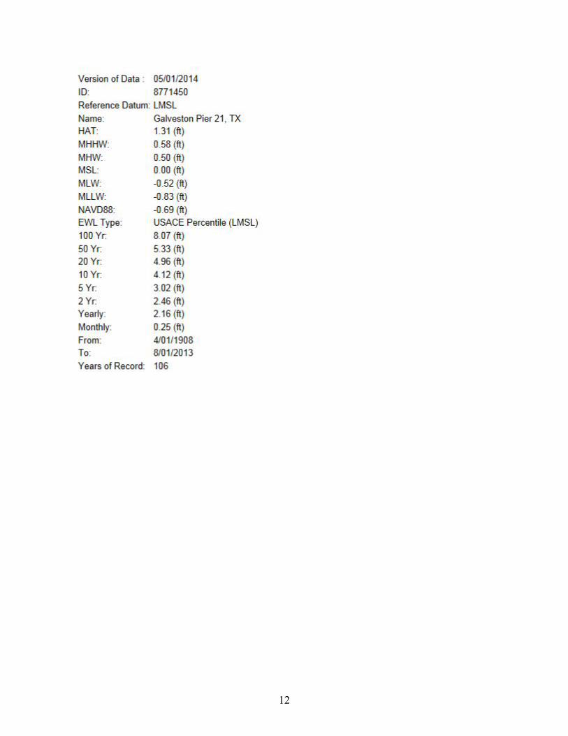
reliable long term. Whether to include decelerating subsidence in final sea levels for the project will be determined in final design phase after more recent sea-level data accumulate. 3.2 HSC “Project Present Condition” Numerical modeling must use the best available data. Unfortunately, these are a combination from datasets and previous model runs in three different years: 2005, 2010, and 2011. The present conditions for the project, for purposes of modeling (ship simulations) are as follows, from the Pier 21 gage, as computed from the USACE sea-level calculator, all referenced to Local Mean Sea Level (LMSL):

Still Water Elevation

Year (ft MSL) Event 1992 0.00 NOAA-defined start point (midpoint of tidal epoch) 2013 0.44 Measured data used by calculator ends at 8/01/2013. 2017 0.52 Year of numerical and economics modeling in this Study 2023 0.65 Anticipated project construction 2073 1.70 End of project 50-year “lifetime” 2123 2.75 End of 100-year planning period The first half of the following table may be used for conversion between datums. The second half shows Extreme Water Levels (EWLs) in construction year 2023 by return period.

12

13

COASTAL GAGES

The following gages on the open coast are listed for comparison purposes. The conclusions are: • On the open coast sea-level rise is faster than in the Bay (6.84 mm/yr vs. 6.39 mm/yr). • Sea-level rise at Galveston’s coast (6.84 mm/yr) is faster than either southwest at Freeport

(4.35 mm/yr) or northeast of Galveston at Sabine (5.66 mm/yr). • A comparison of USACE sea-level rise rates and NOAA rates, based on the same data set,

but over different periods of years, suggests that subsidence is decelerating in Galveston, at a rate of 0.01 mm/yr2.

3.3 Galveston Gulf Side (Pleasure Pier)

The tide gage with sea level trend information nearest to the Galveston coast region, with over 40 years of record, is at the Galveston Pleasure Pier, which is on the Gulf of Mexico coast side of Galveston Island (NOAA Gage #8771510). The NOAA MSL trend (from the Corps’ calculator) at this site (from 1957 to 2008) is equal to 6.84 mm/yr with a 95 percent confidence interval of ± 0.74 mm/yr. If the estimated historic eustatic rate equals that given for the modified NRC curves, the observed subsidence rate would be 5.14 mm/yr (6.84 mm/yr - 1.70 mm/yr).

3.4 Sabine Pass (Upcoast or NE of Galveston)

USACE calculations from NOAA gage #8770570, near the junction of the Sabine River and the Gulf of Mexico, show a sea-level rise of 5.66 ± 0.79 mm/yr computed over 57 years (1958 to 2014). If the estimated historic eustatic rate equals that given for the modified NRC curves, the observed subsidence rate would be 3.96 mm/yr (5.66 mm/yr - 1.70 mm/yr).

3.5 Freeport (Downcoast or SW of Galveston)

The tide gage with sea level trend information nearest to the Brazos River system, with over 40 years of record, is located at Freeport, TX Island (NOAA Gage 8772447). The NOAA MSL trend (from the Corps’ calculator) at this site (from 1954 to 2014) is equal to 4.35 mm/yr with a 95 percent confidence interval of ± 1.12 mm/yr. If the estimated historic eustatic rate equals that given for the modified NRC curves, the observed subsidence rate would be 2.65 mm/yr (4.35 mm/yr - 1.70 mm/yr). 4.0 Predicted Future SLR The Pier 21 tide gage will be used to compute sea level rise for this project, since it is the only one in Galveston Bay with reported sea-level trends, and also has the longest record. In addition to the project design period of 50 years and the project planning period of 100 years, the 25-year period will be calculated, per ETL 1100-2-1, p. C-3.

14

4.1 Predicted Future Rates of RSLC for 25-Year Period of Analysis

The computed future rates of RSLC in this section give the predicted change between the years 2023 (estimated project start date) and 2048 for Galveston Bay. RSLC values for this 25-year period are summarized in Figure 1. For comparison, both NOAA and ACE curves are shown (for this first example only). The rate that will be used in this navigation project is the ACE and NOAA low curve, which are identical since they use the same historic rate. However, the computed elevations from the two calculators differ slightly, since the periods of analysis differ by two years. All curve plots and data tables in this report use the USACE analysis of the NOAA Pier 21 tide gage.

Figure 1: Estimated SLR over the First 25 Years of the Project Life (2023 - 2048)

from both NOAA and Corps of Engineers Curves (Levels are relative to 1992 Zero.)

15

Table 1: Estimated SLR over the First 25 Years of the Project Life (2023 - 2048) (Levels are relative to 1992 Zero.)

For ease of comparison with the 50-year and 100-year periods of analysis, the data from the ACE curves only are plotted here in Figure 2 and listed in Table 2.

16

Figure 2: Estimated SLR over the First 25 Years of the Project Life (2023 - 2048)

Corps of Engineers Curves Only

Table 2. SLR for the 25-Year Period of Analysis (Levels are relative to 1992 Zero.)

17

4.2 Predicted Future Rates of RSLC for 50-Year (Project Design)

Period of Analysis

The computed future rates of RSLC given here assume a 50-year period of analysis, and give the predicted change between the years 2023 and 2073 for Galveston Bay. Relative sea level change values for the 50-year period are shown in Figure 3 and Table 3.

Figure 3: Estimated SLR over the First 50 Years of the Project Life (2023 - 2073)

Corps of Engineers Curves Only (Levels are relative to 1992 Zero.)

18

Table 3. SLR for the 50-Year Period of Analysis (Levels are relative to 1992 Zero.)

19

4.3 Predicted Future Rates of RSLC – 100-year Sea-Level Change

(Planning Period)

The planning, design, and construction of a large water project can take decades. Though initially justified over a 50-year economic period of analysis, USACE projects often remain in service much longer. The climate for which the project was designed can change over the full lifetime of the project to the extent that stability, maintenance, and operations may be affected. These changes can cause detrimental or beneficial consequences. Given these factors, the project planning horizon (not to be confused with the economic period of analysis) should be 100 years, consistent with ETL-1110-2-1. The period of economic analysis for USACE projects has generally been limited to 50 years because economic forecasts beyond that time frame were not considered reliable. However, the potential impacts of SLC over a 100-year period can be used in the formulation of alternatives and for robustness and resiliency comparisons. ETL 1100-2-1 recommends that predictions of how the project or system might perform, as well as its ability to adapt beyond the typical 50-year economic analysis period, be considered in the decision-making process. The initial assessment that evaluates the exposure and vulnerability of the project area over the 100-year planning horizon was used to assist planners and engineers in determining the long-term approach that best balances risks for the project. The three (3) general approaches are anticipatory, adaptive, and reactive strategies. These strategies can be combined, or they can change over the life cycle of the project. Key factors in determining the approach include consequences, the cost, and risk. This consideration is particularly important under a climate-change condition, where loading and response mechanisms are likely to transition over the life of the project. Projected sea-level curves and levels are shown here in Figure 4 and Table 4.

20

Figure 4: Estimated SLR over the First 100 Years of the Project Life (2023 - 2123)

Corps of Engineers Curves Only (Levels are relative to 1992 Zero.)

21

Table 4. SLR for the 100-Year Period of Analysis

(Levels are relative to 1992 Zero.)

5.0 Planning for Sea-Level Rise Note that during the project’s planning period (near the Year 2088), sea level has risen about 2 feet. (NOAA’s inundation plotter will only plot integral numbers of feet of inundation. The 2 ft level happens to occur in year 2088 for this site.) NOAA’s “Sea Level Rise and Coastal Flooding Impacts Viewer” can be used to view the inundation occurring in whole numbers of feet. As seen below in Map 2, it is apparent that much of the land around the East Bay and Trinity Bay is low-lying and therefore inundated.

22

Map 2: Extent of Inundation (light blue) with 2-foot Rise (in year 2088)

Shown in bright green are low-lying areas that are occasionally inundated even before the project start.

6.0 Subsidence Land subsidence in the past has been much higher than in surrounding areas, as shown in Map 3. The main reason is thought to be groundwater extraction, and as a result the Harris-Galveston Subsidence District (HGSD) was formed to monitor and regulate further extraction. As supporting groundwater is removed, sediments compact. There is subsidence of at least a foot throughout this project’s study area. Subsidence has ranged to over 10 feet, and the largest values seem to follow the Houston Ship Channel, from the Turning Basin to the Fred Hartman Bridge (or something similar). Since the Houston Ship Channel Deepening and Widening Project will occur in the future and uses topography that has already been subjected to this historical subsidence, of more concern to this project is future subsidence. Based on HGSD’s planned amounts of future extraction, they have modeled expected future subsidence, plotted here as Map 4. Significantly high values of 0.5 to 1.0 foot are only anticipated significantly far from the Houston Ship Channel. For the channel

23

itself, the effect will be largely beneficial, by deepening the channel. Of more concern are effects on docks and other support facilities.

Map 3: Past Subsidence in Galveston and Harris Counties (from GCCPRD Phase 2 Report, 02/23/2016)

24

Map 4: Anticipated Future Subsidence in Galveston and Harris Counties

(from GCCPRD Phase 2 Report, 02/23/2016) The river in the lower part of the figure (where subsidence can exceed 1.5 ft) is Clear Creek. The river in the upper portion is Houston Ship Channel (where subsidence is

between 0.5 and 1 ft). 7.0 SLR Guidance Specific to Navigation Projects (ETL 1100-2-1’s Appendix C) Appendix C of the ETL “Procedures to Evaluate Sea Level Change: Impacts, Responses, and Adaptation” is titled “Navigation Projects” and specifically addresses only those. The general conclusion about sea-level rise effects on navigation projects is that it is a benefit to the project itself (providing deeper channel water), but is a potential threat or cost to related infrastructure. For federal projects, it is important to know which mitigations or adaptations can be made with federal funds and which cannot. Table 5 below provides general guidance on these two categories. The primary federal structure for HSC is the entrance jetties. Therefore in the numerical model runs and in the with-project ship simulations, it will be important to study the “with sea-level rise” runs effects on the jettied entrance.

25

Deleterious effects on the navigation channel itself can occur however, and three of those areas are listed in the bottom left corner of Table 5. Physically the effect is primarily due to higher waves being able to form and propagate in the deeper channel. Since the deepening planned for HSC will be a relatively small portion of the entire depth, it is expected that this will have little effect and thus not become a risk that the project need address. A clearer quantitative answer to this question should be available when comparing the numerical-model and ship-simulation runs between the “no rise” and “sea-level rise” scenarios. Table 5: Federal and non-Federal navigation project features at risk from sea-level change

(from ETL 1100-2-1 Table C-1)

Table 6 below lists the various physical processes that sea-level rise can affect in navigation projects. The impacts (on the right side of the Table) that are most likely to affect specifically Houston Ship Channel are:

1. Increased ship-wake impacts 2. Vessel excursion and movement 3. Adjacent shoreline change (due to increased propagation of ship wakes) 4. Less dredging needed to maintain the same depth (a benefit) 5. Dredged material placement site capacity

The first three of these should be addressed by the numerical model and ship simulations. The last two should be quantifiable with simpler spreadsheet computations, once this report’s sea-level numbers have been agreed to by the team.

26

Table 6: Physical Processes Sensitive to Sea-Level Rise in Navigation Projects

(from ETL 1100-2-1 Table C-3)

Table 7 below is a qualitative matrix for evaluating the level of risk of sea-level rise to a navigation project. The numerical scores on the left indicate the relative importance of density of each resource in a navigation project. The scores on the right indicate how at-risk that resource is to sea-level rise. Note that the two scores are different. For example, channel dimensions (length, depth, mooring areas) are of high importance or density in the project, but are expected to suffer little impact from sea-level rise. Note that the non-federal port facilities (wharves, docks, etc.) have both a high density and may be at high-risk from sea-level rise. Unfortunately for the local sponsor, sea-level rise scenarios may have much more impact on port facilities than on federal channel dimensions.

27

Table 7: Qualitative Matrix for Determining Risk Level

(from ETL 1100-2-1 Table C-4)

28

7.1 Physical Processes at Navigation Projects affected by Sea-Level Rise (ETL 1100-2-1’s Tables 6 and 8) In deciding which processes should be evaluated for their effects on the project, due to sea-level rise, the following Table 8 provides a checklist to apply to specific projects. Note that the only doubly important marking is for “depth-limited waves”, which means that wave heights can be expected to increase. Within the main channel, the depth increase caused by sea-level rise will be small compared to the total depth, so this effect will be small. However, this is NOT the case with barge lanes and mooring basins, where sea-level rise will be a much larger percentage of the total depth, and where it is known that waves are “depth limited”. (For background information, wave heights are determined by wind speed, but can be limited in three ways: depth, fetch length, and wind duration. There is usually only one of these three factors which controls or “limits” the wave height. In Galveston Bay, waves are usually depth limited.)

29

Table 8: Physical Processes Affected by Sea-Level Rise in Navigation Projects

(from ETL 1100-2-1’s Table 6)

To quantify the effect of sea-level rise on depth-limited wave heights and other factors, Table 9 below provides a useful matrix of specific quantifiable effects. Most of the Table applies to

30

structures. Except possibly at the jetties, the only significant relevance of this Table for this HSC project is that wave height increases in depth-limited (shallow) areas. (The Table’s example shows that the depth-limited wave height increases by the same amount as the sea-level rise, in this case from 6 ft to 6.7 ft.) Corresponding to three different values of sea-level rise, percentage changes are computed for various forces used to compute damaging effects such as wave attack, armor-unit stability, morphology change, and wave run-up on structures and shores.

Table 9: Quantified Changes in Loading Conditions due to Sea-Level Rise (From ETL 1100-2-1’s Table 8)

The numerical model and ship simulations that compare “with sea-level rise” to “without (or present-day)” scenarios should provide quantitative results for estimating the project’s risk to sea-level rise.

31

7.2 SLR Risks and Adaptations for Navigation Projects (ETL 1100-2-1’s Tables 1 and 7) An essential element of developing a good understanding of the project area’s exposure and vulnerability is assessing how quickly the individual scenarios might necessitate an action due to thresholds and tipping points. It is important to identify key milestones in the project timeline when impacts are expected. This involves inputs from all members of the PDT, since the threshold or tipping point could be a variety of different items or combinations of items. Response strategies for the project planning horizon range from a conservative anticipatory approach, which constructs a resilient project at the beginning to last the entire life cycle (and possibly beyond), to a reactive approach, which would simply be to do nothing until impacts are experienced. Between these extremes is an adaptive management strategy, which incorporates new assessments and actions throughout the project life based on timeframes, thresholds and triggers. A plan may include multiple measures adaptable over a range of SLC conditions and over the entire timeline, with different measures being executed as necessitated. For a feasibility-level design, it is important to identify potential cost-risk items and adaptation costs to the stakeholders and decision makers. Further detailed design and analysis may be undertaken during the pre-construction engineering and design phase to optimize project features sensitive to relative sea level change. In this phase, the question of further adaptability beyond the 50-year economic analysis period may be addressed as part of the design optimization. The economic and cost formulation for the project should account for uncertainty in critical design items. Hard structures (rock or concrete) are difficult to alter to accommodate changing conditions, unless they have been designed with that in mind from the beginning. Examples of the three types of approaches are listed below in Table 10. Since this navigation project does not include improvements to hard structures (in the federal part of the project), then it will be relatively easy to design protections and solutions. In contrast, it is difficult to accommodate hard structures that have not been designed from the beginning with adaptation in mind. For example, a dock that has been designed from the beginning with the intention that it will eventually need to be jacked up is much cheaper in the long-run than a dock that has to be torn down and rebuilt. So again, this planning for an adaptive strategy will be much more important to the non-federal part of the project.

32

Table 10: Adaptive Approaches to Navigation Projects

(From ETL 1100-2-1’s Table 1)

In planning an adaptation strategy, Table 11 below provides a useful method of selecting the kind of adaptation to use (P = Protect, A = Accommodate, R = Retreat) and also provides a list of specific solutions to pick from. Both the kind of adaptation and specific solutions are shown in the right-most column. The two categories of sea-level effects in the left-most column that are more likely to affect this project are “wetland loss” (federal) and “infrastructure damage” (non-federal). Therefore both the entire team and the non-federal team should plan their adaptation strategies.

33

Table 11: Systems Affected by Sea-Level Rise and Adaptation Approaches

(From ETL 1100-2-1’s Table 7)

34

8.0 Recommendations As a conservative approach (not exaggerating benefits from sea-level rise), USACE’s Low Sea-Level Curve should be used for the navigation portion of this project. Including sea-level rise and subsidence in the project design will result in less dredging than otherwise anticipated, since the channel depth is increasing due to both of these factors. At the end of the 50-year project life, channel depth will have increased (since construction) by: 1.70 ft (in 2073) – 0.65 ft (in 2023) = 1.05 ft. At the end of the 100-year planning period, channel depth will have increased (since construction) by: 2.75 ft (in 2123) – 0.65 ft (in 2023) = 2.10 ft. If sea level rises faster than the historic “Low” rate, then channel depth will increase even more. Conversely, SLC effects on the non-federal sponsor’s infrastructure will largely be detrimental. They should carefully consider which sea level to plan for, and more importantly, what their adaptation measures should be (Table 11). Some deleterious effects due to sea-level rise may also occur within the federal project. Many of the general categories of effects listed in the Tables will not apply to this project, but most likely there will be some deleterious effects in some of the following categories: Increased erosion at islands Increased ship wakes in barge lanes and mooring areas Increased wind waves, especially in shallow areas (but not in the main channel) Changes in water chemistry (salinity, dissolved oxygen) For the first three items in the list above, some simple spreadsheet calculations can be performed to indicate a level-of-concern. For all four categories, the numerical model and ship simulation runs should help quantify the effects. One decision the team will have to make is which scenarios are to be run in the model and in the simulations. There are not likely to be sufficient funds to run all possible combinations of: Low, Intermediate, and High SLR; their effects on multiple ship sizes; and runs both with and without project. The current plan is to make four runs: Present Condition, Project TSP, Project Alternative, and Future with TSP. The primary federal structures for HSC are the entrance jetties. Therefore in the numerical model runs and in the with-project ship simulations, it will be important to study the effects of “with sea-level rise” on the jettied entrance.

35

References ER (Engineering Regulation) 1100-2-8162, “Incorporating Sea Level Change in Civil Works Programs”, 31 Dec 2013, 3 pp + 2 Appendices. ETL (Engineering Technical Letter) 1100-2-1, “Procedures to Evaluate Sea Level Change: Impacts, Responses, and Adaptation,” 30 Jun 2014, 5 Chapters + Appendices A-G.

36

(This page left blank intentionally.)