1 Casino Revenue Sensitivity to Competing Casinos: A Spatial Analysis of Missouri Douglas M. Walker* College of Charleston Todd M. Nesbit The Ohio State University March 25, 2013 Forthcoming, Growth and Change (2013) Abstract: Previous studies have examined the relationships among different gambling industries (e.g., casinos, lotteries, and racetracks), with mixed results. Yet, the literature lacks evidence on the extent to which casinos in a particular market compete with each other. No study considers the proximity of competing casinos in its empirical analysis. This analysis uses quarterly casino property-level revenue data from Missouri, 1997.1 to 2010.2, and a model with a distance-adjusted competition scalar to analyze how competing casinos affect the revenues of a particular casino. The results indicate that machine games, table games, and square footage all have a positive effect on own-casino revenues. Machine games and square footage have a negative impact on competing casinos; however, table games have a positive impact on competing casinos. These results are consistent with how the Missouri casino industry is developing, with more emphasis on machine games and less on table games. The results suggest that casinos are competitive in nature (i.e., are substitutes), as there is no evidence to suggest that there is any positive agglomeration effect from casinos being clustered. This analysis should be of interest to industry and policymakers, and provides a foundation for further research on the U.S. casino industry. JEL codes: L83, Industry Studies: Services, Gambling R12, Size and Spatial Distributions of Regional Economic Activity Keywords: Casino competition, Spatial analysis, Regional economic analysis * Corresponding author. Email [email protected]
Transcript
1
Casino Revenue Sensitivity to Competing Casinos:
A Spatial Analysis of Missouri
Douglas M. Walker*
College of Charleston
Todd M. Nesbit
The Ohio State University
March 25, 2013
Forthcoming, Growth and Change (2013)
Abstract: Previous studies have examined the relationships among different gambling
industries (e.g., casinos, lotteries, and racetracks), with mixed results. Yet, the literature lacks
evidence on the extent to which casinos in a particular market compete with each other. No study
considers the proximity of competing casinos in its empirical analysis. This analysis uses
quarterly casino property-level revenue data from Missouri, 1997.1 to 2010.2, and a model with
a distance-adjusted competition scalar to analyze how competing casinos affect the revenues of a
particular casino. The results indicate that machine games, table games, and square footage all
have a positive effect on own-casino revenues. Machine games and square footage have a
negative impact on competing casinos; however, table games have a positive impact on
competing casinos. These results are consistent with how the Missouri casino industry is
developing, with more emphasis on machine games and less on table games. The results suggest
that casinos are competitive in nature (i.e., are substitutes), as there is no evidence to suggest that
there is any positive agglomeration effect from casinos being clustered. This analysis should be
of interest to industry and policymakers, and provides a foundation for further research on the
U.S. casino industry.
JEL codes: L83, Industry Studies: Services, Gambling
R12, Size and Spatial Distributions of Regional Economic Activity
Since the late 1980s state governments have been legalizing commercial casinos as a
strategy to promote employment, tax revenues, and economic growth. Although there still has
not been much academic research on the economic impacts of casinos, there is some evidence
that casinos do promote economic growth and employment (Walker and Jackson 2012; Cotti
2008). Casinos have become widespread in the U.S. By the end of 2011, the U.S. had over 900
commercial and tribal casinos and at least 47 racetrack casinos (“racinos”) operating in 38 states
(AGA 2012).
State government interest in legalizing or expanding commercial casinos increased upon
the onset of the recession in late 2007. Kansas, Ohio, and Massachusetts have legalized casinos,
and several other states are in the process of doing so or of expanding their existing industries.
Total national industry revenues continue to increase as the number of casinos increases (AGA
2012).1
Despite the apparent importance of casinos as a part of state governments’ fiscal policies,
little research has been published on the intra-industry relationships among casinos. It is not
obvious whether casinos complement each other through an agglomeration effect, or whether
they act as substitutes to each other. The casinos in Las Vegas, Atlantic City, and Biloxi certainly
benefit from being clustered. Yet, most states to legalize casinos recently have followed a
“regional model” – allowing only one casino in each region of the state (e.g., Kansas, Ohio, and
1 There was a decline in revenues during the recession of 2007-09, but nationally revenues have been increasing
since 2009.
3
Massachusetts). Clearly, the intra-industry relationship between casinos is an important issue,
given that politicians in each state explicitly control the size and locations of casinos.
As an indication of the importance of the issue, consider that the Missouri Gaming
Commission invited a policy analysis of the likely impact of introducing a 13th
casino into the
state’s existing market. The 2010 report suggested that the smaller and more isolated the casino,
the more positive its effects would be on employment, gaming revenues, and tax revenues for the
state (Missouri Economic Research and Information Center 2010).
Interestingly, the MERIC report asserts that because the Kansas City casinos are in close
proximity to each other (within 5 miles of each other), “any new casino located near existing
competitors in Kansas City will cannibalize [Adjusted Gross Revenue] to a high degree”
(Missouri Economic Research and Information Center 2010). In one “best case” scenario
estimate of a new casino development in an urban Missouri casino market, the model still
assumes cannibalization amongst casinos. “No cannibalization” is only considered to be a
possibility if a casino is isolated from other casinos. Any agglomeration benefit from casinos
clustering is not acknowledged. Yet, this assumption that casinos must be competitors and not
complementary (in terms of revenues) seems inconsistent with several mature casino markets
which have seen net growth even as the number of casinos in the market increased. Obvious
examples include Las Vegas, Biloxi, and perhaps even the Kansas City and St. Louis markets.
The purpose of this study is to test whether relative casino location and competing casino
size affect a particular casino’s revenue. The empirical analysis helps address the inter-industry
relationship among casinos and may be informative as to whether a “clustered” or “regional”
strategy is better for locating casinos. The results indicate that increased regional competition –
through increased machine games and/or square footage of competing casinos, or through
4
reduced distance to competing casinos – has a negative impact on a particular casino’s revenues.
The analysis focuses on Missouri, but the model could be applied to other states, regions, and
countries. An understanding of how sensitive a casino’s revenues are to other casinos’ locations
and sizes should be valuable to the casino industry, policymakers, voters and regulators debating
whether to introduce casinos or to expand existing casino markets.
The paper is organized as follows. The remainder of this section briefly reviews the
literature. Section II is a description of the Missouri casino market and the data used in the
analysis. Section III explains the model and presents the results. Section IV discusses the
predicted impact of a new casino in the Missouri market. A robustness check of the OLS model
is presented in Section V, and Section VI concludes.
Literature review
Several studies have examined the determinants of casino legalization. These include
Furlong (1998), Calcagno, et al. (2010), Richard (2010), and Wenz (2008). However, none of
these studies examines how casino revenues will be impacted by adding a new casino or
changing existing casinos’ capacities.
There have been a few studies that have directly or indirectly examined inter- and intra-
industry relationships among gambling industries, with a particular focus on casinos. Walker and
Jackson (2008) found that within a particular state, tribal casino square footage has a positive
impact on commercial casino revenues, indicating complementary. However, in testing the
impact of adjacent state casinos, they found a negative impact of casino revenues on neighboring
state casino revenues, indicating substitution. Although these results are certainly relevant to the
5
issue in this paper, their analysis was aggregated to a national level, using state-level data, rather
than property-level data.
Several other papers have examined the substitution issue. Anders et al. (1998) found that
Indian casinos harm other forms of entertainment. Elliot and Navin (2002) concluded that
casinos and pari-mutuels harm lotteries, while Siegel and Anders (1999, 2001) found that casinos
harm other forms of entertainment, slot machines harm the lottery, and that pari-mutuels do not
affect the lottery.
The study by Thalheimer and Ali (2003) examined slot machine handle at casinos in
Iowa, Illinois, and Missouri, from 1991-98. They model competition among casinos by
introducing a variable measuring “ease of access” to casinos from the county’s population, which
is assumed to be located at the geographical centroid of the county (p. 917). Unsurprisingly, they
find that as potential customers’ access to casinos increases, the demand for casino gambling
increases. In addition, they find that demand at a particular casino decreases when access to
competing commercial casinos, racinos, or tribal casinos increases (p. 914).
A recently published study by Condliffe (2012) examines how the introduction of casinos
in Pennsylvania has affected overall revenues in the regional market of southeast Pennsylvania,
Delaware, and Atlantic City. He finds that the introduction of casinos in Pennsylvania reduces
total revenues in the region, and that an increase in the number of slot machines in Pennsylvania
reduces overall regional revenues. McGowan’s (2009) study, which looks only at Pennsylvania
and New Jersey, finds that total revenues in the states increased when Pennsylvania introduced
casinos. Although these studies do not address the substitution issue directly, they provide
interesting analyses of expansion in the Northeast casino market.
6
Other papers in the literature examine the casino industry, but there is no study that
focuses on the property-level relationship between casinos. This study will therefore be a useful
contribution to the literature.
II. Data
In order to test whether (and how) casino revenues depend on the size and proximity of
other casinos, one must first specify a market to analyze. Many states that have commercial
casinos also have casinos owned by Indian tribes. Since Indian tribes are sovereign nations, their
casino revenues are generally not public information. Because of this, a good empirical analysis
that focuses on casino revenues is difficult to perform in states that also have tribal casinos.
Missouri does not have tribal casinos; it therefore represents an ideal and unique case study for
how casinos affect each other. This section provides a background of the Missouri casino
industry and presents the data used in the analysis of the market.
Background on Missouri
Missouri was the sixth state in the U.S. to legalize commercial casinos, in 1993, and
riverboat casinos began operating there in May 1994 (Calcagno, Walker, and Jackson 2010). As
of December 2012 there were 13 commercial casinos operating in the state, with the newest
casino opening in late October, 2012 (Miller 2012). By state law, Missouri can have a maximum
of 13 riverboat casinos (Missouri Economic Research and Information Center 2010). Riverboat
casinos were initially required to “cruise” while customers gambled. However, in 1998 the
cruising rule was eliminated and now regulations only require that “Missouri riverboat gaming
7
casinos must be located within 1,000 feet of the main channel of the Missouri and Mississippi
rivers.” Casinos can now be riverboats, “boats in moats” or land-based.2
An overview of the Missouri casino market at the end of 2011 is presented in Table 1.
The table lists the city/market, casino name, opening date, major changes in ownership, and
closures. The four right-most columns list measures of casino size and activity: adjusted gross
revenues (AGR, the revenue the casino keeps after paying winning bets to customers), casino
floor area in square feet, and the number of table games and machine games operating in each
casino during 2011. “Table games” include baccarat, craps, blackjack, poker, etc. “Machine
games” include slot machines, video poker, video lottery terminals, and any other electronic
gambling devices. Note that Table 1 also lists this information for the two casinos (Sam’s Town
and President) that have closed, along with one casino that was merged with another casino
(Players Casino merged with Harrah’s Maryland Heights).
[Table 1 here]
The Missouri casino industry has expanded fairly consistently since its birth in 1994.
Figure 1 lists the industry revenues by fiscal year and the number of casinos operating in the
state for at least half of the fiscal year. Revenues increased at a fairly constant rate for the first 10
years, and more recently at a decreased rate. Revenue growth has slowed during a time when the
number of casinos was fairly stable at 11 and 12.
[Figure 1 here]
2 For more on the evolution of regulations, see the Missouri Gaming Commission website, mgc.dps.mo.gov/.
8
As an industry, legalized gambling is not a very large contributor to U.S. state coffers.
Walker and Jackson (2011) show that in 2004 only four states received more than 5% of their
government revenues from legalized gambling. In Missouri 3.3% of state revenue is from
legalized gambling (2.1% from casino taxes, 1.1% from lottery receipts). Overall, while casinos
may not represent a critical source of state revenues, casino taxes do allow politicians to avoid
making unpopular decisions, at least at the margin, such as (non-casino) tax increases or
spending cuts.
Missouri provides an ideal casino market for our analysis because during the sample
period new casinos open, old ones close, and several casinos expand in size at least once.
Therefore, it is possible to model how such changes in competition affect any particular casino’s
revenues.
When the President Casino in St. Louis closed in 2010, it freed up a license for a new
entrant into the market. Policymakers were interested in whether it would benefit the state, or the
state’s casino industry, to allow a new casino to open in the place of the President Casino. The
state commissioned a study of the likely impacts on existing casinos prior to approving a new
casino license. The same issues confronted by Missouri – whether to expand the casino industry,
and where a new casino should be located – confront every state with casinos or considering
legalizing them. Will adding a new casino to a market improve or worsen overall industry
performance and tax receipts? And how do casinos’ relative sizes and locations affect each
other? Since this is one of the first papers to analyze these issues, it fills an important gap in the
casino literature.
9
Data
The goal of the analysis is to model how location-specific casino revenues are impacted
by changes in regional competition. Regional competition is defined as those casinos,
commercial or tribal, operating within 100 miles of each casino. Using this range requires that
several casinos outside of Missouri be considered, including casinos in Illinois, Kansas, and one
in Iowa. All of the casinos that are included in the analysis are illustrated in Figure 2. Also
shown in the figure is Harrah’s Tunica Casino, which lies at the very edge of the 100-mile
distance from the Lady Luck Casino in Caruthersville. The Tunica casino is not included in the
analysis, but it is shown on the map to give a visual of the next closest casino.3
[Figure 2 here]
As noted above, the dependent variable is a measure of casino activity: casino property-
level adjusted gross revenues (AGR).4 Casino revenue data were provided by the Missouri
Gaming Commission, and were adjusted for inflation using the CPI. The study uses quarterly
revenue data for all Missouri casinos that were open for the entire period from 1997.1 through
2010.2.5 This encompasses data on nine casinos for 54 quarters. (These casinos’ names are
shaded in Table 1.) The purpose of the analysis is to examine how existing casinos are affected
3 Thalheimer and Ali (2003) estimate that only 4% of visitors come from more than 100 miles away from a casino.
This estimate is based on 1997 Illinois data. Since there has been significant expansion of casinos since then, it is
unlikely that Tunica would impact any Missouri casinos. 4 One referee suggested that the model should be run using per capita casino revenues as a dependent variable. This
was done, and the results are not markedly different from those presented. It is acknowledged that the analysis could
also be done using number of casino patrons, rather than revenues. The main reason to use revenues is that, as a
matter of policy, politicians and voters are more concerned with the tax revenues raised by casinos, and not by the
number of customers. Although the state does charge an admission tax, the great majority of its revenues from
casinos come from the tax on gross gaming revenues. Using revenues seems to be the most direct way to examine
the relationships among casinos. 5 Several casino closings were reported, usually due to flooding. These closures lasted an average of about two
weeks. However, given the data are quarterly revenues, the closings are relatively minor and are not accounted for in
the analysis.
10
by other casinos opening, closing, or changing in size. The goal is not to explain revenues for
casinos that newly opened or closed down during this time period or to explain why casinos open
or close. Therefore, casinos that opened or closed during the sample period are not included in
the dependent variable. However, opening and closing casinos’ size and location data are
included in the relevant explanatory variables.
The explanatory variables in the model include measures of the scale of operation of each
casino, measures of regional competition, and regional demographic measures to account for
demand. The model considers casinos operating within 100 miles of each Missouri casino as
regional competition. Some competing casinos are located in Kansas, Illinois, and Iowa, and data
on these casinos are included with the explanatory variables.6 The distances between casinos are
calculated “as the crow flies,” and are derived using the longitude-latitude coordinates based on
the casinos’ physical address, as determined in Arc GIS 9.3. The casinos’ physical addresses are
available from CasinoCity (casinocity.com).
There are two measures of scale. The first is the number of table games and number of
machine games at the casino. The second measure is the casino’s square footage. These scale
data are reported on an annual basis. The competition measures for each included Missouri
casino are computed based on all operating casinos within 100 miles, for each sample year.
Scale data for Illinois casinos are provided by the Illinois Gaming Board’s Annual
Reports, 1999-2011.7 Kansas casino data comes from the Kansas State Gaming Agency
(www.accesskansas.org/ksga/) and CasinoCity. A Kansas State Gaming Agency official
6 Non-Missouri casino revenue data are not included on the left-hand-side of the model. This is because the focus
here is on the Missouri casino market in particular. Also, several of the casinos outside Missouri are tribal casinos,
and revenue data are not available for those. 7 See www.igb.state.il.us/annualreport/. Reports are not available prior to 1999. However, the Public Information
Officer of the Illinois Gaming Board indicated that there were no significant changes to the three casinos in the 100-
mile competition threshold from their openings through 1998. For 1997, 1998 values are used, which were reported
in the 1999 annual report.
11
confirmed there had been no significant expansions to the casinos in the 100 mile competition
region during the sample period, with the exception of that at Sac & Fox, in 2008. Finally, data
for the relevant casino in Iowa was collected from the Iowa Racing and Gaming Commission
website (www.state.ia.us/irgc/).
The pairwise distance with each Missouri casino is calculated and used to compute two
gravity-model inspired regional competition variables, which are label as Distance-Scaled
Competition (DSC) for modeling purposes. These variables incorporate both distance and the
competing casino scale in its calculation. Hall, Lawson, and Skipton (2011) use a similarly
proximity to world concentrations of demand” in their model of international trade. Likewise,
Nesbit and Lawson (2012) construct a Distance Scaled Tax Differential variable in their model
of cigarette smuggling.
For each Missouri casino i data are collected on the number of table games and number
of gaming machines for all other j casinos within 100 miles. These measures are scaled
individually by in one specification and by in another, and then the scaled
measures are summed. Thus:
for all i = 1…n (1)
and for all i = 1…n (2)
Sizej represents one of the measures of casino size (table games, machine games, square footage).
Distance is measured as the “as the crow flies” distance between casinos. An increase in regional
12
competition would be represented by an increase in DSC. This could occur through an increase
in the size of a nearby casino (either in square footage, number of machines, or number of
tables), the relocation of an existing casino to a closer venue, or the opening of a new casino
within a 100 mile radius.
The remaining demand factors considered include real per capita personal income
(PCPI), the unemployment rate (Urate), and estimated population (Pop) in the Metropolitan
Statistical Area (MSA) within which a casino is located or that is closest to the casino.8 The
Kansas City MSA includes five casinos in the analysis; the St. Louis MSA includes six casinos
in the analysis. There is one casino in the St. Joseph MSA. The remaining casinos in the state are
not in MSAs. Since the goal in using MSA-based data is to represent the local demand for
casinos, for the relatively isolated casinos the closest MSA or Micropolitan Statistical Area are
used for the data. Boonville is in the county adjacent to the Columbia MSA. La Grange is closest
to the Quincy, IL Micropolitan Statistical Area, and Caruthersville is closest to Dyersburg, TN.9
8 An additional factor that was tested, but is not included in the model presented here, is the smoking ban that was
implemented in Illinois on January 1, 2008. When a smoking ban dummy variable is included for the St. Louis
casinos that would most likely be affected, the impact of the Illinois smoking ban was negative on the Missouri
casinos. This unlikely result probably indicates that the dummy is picking up something else happening in St. Louis.
Or, the negative Illinois smoking bank effect could be possible if the traffic of non-smoking Missourians going to
Illinois casinos was greater than the traffic of Illinois smokers coming to Missouri casinos. This is unlikely, but it is
worthy of further investigation. In any case, the smoking ban variable did not markedly affect any other coefficient
estimates in the model. 9 One reader of the paper suggested that the distance from the casinos to the relevant population center be used to
model casino demand, rather than using the distance between casinos. This would seem to help explain a particular
casino’s revenues, as most of the casinos’ revenues likely come from nearby customers. However, in order to model
the casino market in this way, one must assume that the population exists at one particular point in the casino
market. Since the casinos in St. Louis and Kansas City are fairly close to each other, this type of model would not be
expected to provide particularly interesting or meaningful results. Furthermore, a recent study has shown that most
people do not visit the closest venue most of the time, although machine gamblers do so more than non-machine
gamblers (Young, Markham, and Doran 2012). This evidence suggests that using the population centroid as the
main determinant of demand may be inappropriate.
13
Annual population estimates are from the Census Bureau. Annual unemployment rate
data are from the Bureau of Labor Statistics. Annual per capita personal income data are from
the Bureau of Economic Analysis.10
Personal income data are adjusted for inflation with the CPI.
III. Model and results
The goal of the analysis is to determine the extent to which competing casino size and
proximity affects a particular casino’s revenues. Quarterly real casino revenue at the property-
level is used as the dependent variable. Explanatory variables include measures of scale of each
Missouri casino, measures of competing casinos within 100 miles of each particular casino
(DSC), and the demographic variables of MSA population, unemployment rate, per capita
personal income, and property-level fixed effects. The model is shown in equation (3):
(3)
The natural log of each variable (except unemployment rate) is used. In addition the model
includes two-way fixed effects.
Four specifications of the model are tested: a pair employing both gaming machines and
tables games as the casino size and competition variables and another pair of specifications
instead employing casino square footage. Within each aforementioned pair, the method by which
competition is scaled is varied: first scaling competition by distance and the second scaling
competition by distance-squared. Two scaling methods are used for the competition variables to
not only show robustness but also because theory does not suggest a specific competitive decay
function. As will be described more fully below, the choice of the scaling does not significantly
10
2010 estimates for some regions are based on the prior two years’ average rates of change.
14
impact the qualitative interpretation of our results. The below discussion emphasizes the
distance scaled (rather than distance-squared scaled) results; this choice is largely based on
interpretive convenience.
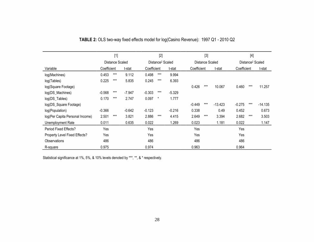
Ordinary least squares (OLS) results of the four specifications are presented in Table 2.
The results shown are for a two-way (quarter and casino property) fixed effects model. Columns
1 and 2 present the specifications in which gaming machines and tables are used; columns 3 and
4 present the square footage specifications. The distance scaled specifications are presented in
columns 1 and 3; while columns 2 and 4 show the results in which distance-squared scaled
competition measures are used.
[Table 2 here]
The gaming machine and table game models (columns 1 and 2) are discussed first. In
both specifications, the coefficients on the log(Machines) and log(Tables) variables are positive
and statistically significant, indicating that an increase in the number of gaming machines or
table games at a given casino will increase revenues at that casino. More specifically, using the
results in column 1, a ten percent increase in the number of machines is associated with a
roughly 4.5 percent increase in revenues at that casino. The elasticity of casino revenue with
respect to gaming tables is approximately half that of gaming machines. That is, a ten percent
increase in the number of table games is explained to increase the casino’s revenues by 2.25
percent.
The two distance-scaled competition variables, DS_Machines and DS_Tables, are both
found to be statistically significant determinants of casino revenue in both OLS specifications
presented in Table 2, columns 1 and 2. The results in column 1 indicate that a ten percent
15
increase in Distance Scaled Machines is estimated to reduce revenues at a specific casino by
about 5.7 percent while the same percentage increase in Distance Scaled Tables is estimated to
increase casino revenue by 1.7 percent. The results in the Distance-squared Scaled specification
are qualitatively similar: an increase in Distance-squared Scaled Machines is estimated to
decrease casino revenue while an increase in Distance-squared Scaled Tables is shown to
increase casino revenue. These results indicate that consumers view gaming machines at nearby
casinos as substitutes for those at a given casino. However, an increased availability of table
games, whether it be through a greater number of tables or tables which are located
geographically closer to a given casino, can be explained to be weak complementary goods.
The complementary effect of table games may be because gamblers value the option to
move to another casino when on a “cold” streak on the table games at a given casino. Machine
gamblers, on the other hand, may interpret an extended period of losing on a given machine as
increasing the odds that the next pull will reward them with a jackpot. Thus, these gamblers often
sit at the same machine (or small group of machines) in the same casino for an extended period
of time. Further, given that each casino has many variations of machine games, there is little
need to leave the casino for a new experience when such a change is desired by the player.
Alternatively, one can think of the table game result to mean that a decrease in table
games in one casino leads to lower revenues at competing casinos. Since the trend in Missouri
casinos over our sample period has been to reduce casino floor space dedicated to table games,
while expanding floor space dedicated to machines, this result here seems consistent with how
the casino market has been developing, for example, as found by Levitzky, Assane, and
Robinson (2000).
16
The specifications presented in columns 3 and 4 of Table 2, in which square footage
replaces the use of gaming machines and table games, generate similar results as those discussed
above. First, an increase in a casino’s square footage, ceteris paribus, is shown to increase the
casino’s revenue. More specifically, a ten percent increase in square footage is estimated to
increase that casino’s AGR by 4.3 percent, according to the results presented in column 3. The
existence of nearer and larger casinos is shown to reduce revenues at any given casino. That is, a
ten percent increase in Distance Scaled Square Footage is estimated to reduce casino revenues by
nearly 4.5 percent (column 3). This is consistent with the results discussed above in regards to
Distance Scaled Machines, and suggests that the effect of competing machine games dominates
the effect of greater regional availability of table games.
To summarize, the results from the OLS model suggest that casinos are sensitive to
competing casinos. An increase in a casino’s square footage or number of machine games is
found to cause a decrease in the revenues at competing casinos. However, a decrease in a
casino’s table games is found to decrease revenues at competing casinos. Next the model is used
to predict what would happen if a new casino were to be introduced in Missouri.
IV. Predicted impact of a new casino
Whether to introduce a new casino was the decision faced by the Missouri Gaming
Commission after the President Casino closed in 2010, and it is a decision gaming regulatory
agencies across the country will likely face at some time. An interesting extension to the analysis
is to consider the model’s predicted impact of a new casino being introduced to the Missouri
market.
Three possible locations for a new (fictional) casino are considered:
17
St Louis (near the intersection of 4th
Street and Spruce Street)
Caruthersville (near the intersection of Truman Boulevard and 3rd
Street)
Cape Girardeau (near the intersection of Broadway Street and Spanish Street Court)
Each of the three locations are depicted in Figure 2 and are denoted by a blue star. The
first two locations are chosen somewhat randomly, solely in order to compute distances to each
of the other existing casinos in the state; they are not intended to be realistic proposed sites.
Relocating the sites by a few miles will have little influence on the estimated impacts presented
below. The Cape Girardeau location, however, is the actual location of the new casino that
opened in October 2012. The predicted impact of each fictional casino is considered
independently.
For the first two fictional casinos, the size is set as the average size of the existing St.
Louis casinos as of the second quarter of 2010, the last period included in the sample. As such,
the casino is assumed to be 93,000 square feet with 2,042 gaming machines and 52 table games.
For the Cape Girardeau casino, the casino size is that which was approved by the Missouri
Gaming Commission for the Isle Casino Cape Girardeau that now operates there: 38,500 square
feet, with 1,000 machine games and 28 table games (Missouri Economic Research and
Information Center 2010, p. 11). There are only two Missouri casinos within 100 miles of the
Cape Girardeau casino: the President Casino in St. Louis, and the Lady Luck in Caruthersville.11
The influence of the new fictitious casino is, by construction within the model, limited to
those casinos within 100 miles. Further, only three of the St. Louis casinos (Harrah’s St. Louis,
Ameristar St. Charles, and President) are included in our full sample, limiting the measured
11
Recall that the President Casino is now closed, but it was open during the entire sample period. The results are
still informative, as they can be interpreted as the impacts on a casino similar to the President in the St. Louis
market.
18
impact of the new St. Louis casino to those three casinos. There is no other casino in Missouri
within 100 miles of the Lady Luck in Caruthersville; thus, the impact of the proposed
Caruthersville casino will be limited to the Lady Luck. There are two Missouri casinos within
100 miles of the Cape Girardeau casino (the President, in St. Louis; Lady Luck, in
Caruthersville).
Table 3 presents the predicted impact of the three fictional casinos on existing casinos in
Missouri. The estimates are based on 2010.2 data and are generated from the results presented in
Column 1 of Table 2.
[Table 3 here]
The new casino in St. Louis has a predicted negative impact on the three St. Louis casinos’
quarterly revenue, averaging about $316,000 per casino. As the Harrah’s and Ameristar
properties had revenues between $70 and $75 million during that quarter, the new casino is
predicted to have very little effect on their revenues. This is likely because those two casinos are
about 20 miles away from the fictional new casino. The President casino, on the other hand, is
about 1 mile away from the proposed casino, and the predicted decrease in revenues for that
casino is about 3%. This predicted impact on The President’s revenues is less than expected, but
overall these results do suggest that St. Louis is large enough a market to host another casino.
The predicted impact of the Caruthersville and Cape Girardeau casinos are intriguing.
The new casino in Caruthersville is predicted to reduce the existing Lady Luck’s revenues by
$3.3 million, or about 40%. This large effect is due to the fact that the new casino dramatically
changes the distance-scaled competition variables, and suggests that the Caruthersville market is
19
not large enough to support two casinos so close together. The fictional casino in Cape Girardeau
is predicted to have a positive impact on the Lady Luck in Caruthersville. While this result is
surprising, one possible explanation of this effect is that the new casino may help to attract more
tourists to the Southeast region of Missouri, and both casinos benefit as a result. (This
explanation may not reconcile well with the prediction that another casino in Caruthersville
harms the casino already there.) While the primary (distance-scaled) specification does predict a
positive impact on Lady Luck, the distance squared-scaled specification from Column 2 of Table
2 does suggest a reduction in Lady Luck revenues. The primary difference is this result likely
stems from the fact that the distance squared-scaled specification discounts more distant
competition more heavily than does the distance-scaled specification. The new casino in Cape
Girardeau is also predicted to have a very minor, insignificant, impact on the President Casino in
St. Louis.
Overall, the estimated impacts of the new casinos of Table 3 based on the OLS
specification presented in Column 1 of Table 2 are robust to other specifications of the model.
For instance, the presented specification predicts a 0.66 percent reduction in existing casino
revenue in response to the new St. Louis casino; this impact is reduced to a 0.03 percent
reduction based on the distance-squared specification of Table 2, Column 2. The two
specifications produce an almost identical predicted change in existing casino revenue in
response to a new Caruthersville casino: -2.30 percent versus -2.27 percent. The Cape Girardeau
casino results produce a more significant difference. The distance-scaled specification suggests a
1.17 percent increase in existing casino revenue, whereas the distance squared-scaled
specification indicates a 0.34 percent reduction. The specifications in Columns 3 and 4 of Table
2 also produce estimated revenue impacts similar to those discussed above.
20
While the new casinos’ predicted impacts are questionable, the analysis here does
provide a foundation for future research into the intra-industry relationships among casinos.
Despite the predictions above, the OLS model results are robust with respect to the estimation
procedure, as discussed in the following section.
V. Robustness check: Spatial Durbin model estimation
As a robustness check of the OLS two-way fixed effects results discussed in Section III,
the model is re-estimated using a Spatial Durbin Model estimation procedure. A growing body of
literature suggests that OLS estimates in studies employing cross-sectional or panel data may
suffer from spatial dependence; see, for example, LeSage and Dominguez (2012), Lacombe and
Shaughnessy (2007), and Hall and Ross (2010). In such circumstances, the coefficient estimates
are biased and/or inconsistent depending on whether the spatial dependence arises in the
dependent variable and/or the error term. Various methods of modeling spatial dependence exist,
but LeSage and Pace (2009) argue that the SDM is superior to the spatial autoregressive (SAR)
and spatial error model (SEM) for many, if not most, applied situations.12
The authors present a
purely econometric argument for the use of the SDM, that the SDM greatly reduces omitted
variable bias when the omitted variable(s) are not only correlated with included independent
variables but also vary systematically over space.13
The SDM includes both a spatial lag of the dependent variable ( ) and the spatial lag
of the explanatory variables ( ), as described in Equation 4:
(4)
12
This argument is further emphasized in LeSage and Dominguez (2012). Also see McMillen (2010) for a
discussion of spatial modeling. 13
In this case, such an omitted variable could include, among others, un-measurable social norms and preferences
regarding gambling, which are not fully captured by per capita personal income and the unemployment rate.
21
where is assumed to be well behaved: . is interpreted as the weighted average
of the explanatory variables of neighboring casinos. For example, the spatial lag of the PCPI
variable is interpreted as the average PCPI of the identified neighboring casinos.
The use of a spatial model necessitates the creation of the row standardized spatial weight
matrix, . The two most common methods of determining the spatial weight matrix are: 1) m
(often m is chosen as 5 or 10) closest neighbors, and 2) those other properties within a specified
distance. Given that there are only 9 cross sectional units in the study, the first option is not
reasonable. As such, the second option is chosen, but this, too, requires the determination of the
appropriate distance. In the current analysis neighbors are defined as the other Missouri casinos
which are within 100 miles.14
The SDM model is estimated in Matlab, employing LeSage’s Spatial Econometrics
Library and calling the “sar_panel_FE” function based on Elhorst (2003, 2010). The model is
estimated including both period and property-level fixed effects. Interpreting the estimates from
any model including on the right-hand-side is more complicated than simply looking at the
estimated coefficient as was done above in the OLS case. This is because the partial derivative
with respect to a given independent variable is an n x n matrix rather than a scalar (LeSage and
Dominguez 2012). In order to interpret such estimation results, one must compute the direct and
indirect effects (impacts), a process that is described in LeSage and Pace (2009). The direct
effects are interpreted as the own effects – how a given change in an independent variable for a
specific casino impacts revenues for that same casino (including all feedback). The indirect
effects can be interpreted as the combined spillover effects on all other Missouri casino revenues.
The total effects are the sum of the direct and indirect effects.
14
No other Missouri casino is within 100 miles of Lady Luck in Caruthersville; however, the spatial econometric
model requires that each cross-section have at least one neighbor. As such, the closest Missouri casino, the President
Casino, is assumed to be the sole neighbor of Lady Luck.
22
While the full results – coefficient estimates, direct effects, indirect effects, and total
effects – are available in an unpublished appendix (and available from the authors upon request),
only the direct effects are presented in Table 4, as these are the results which are most relevant to
computing the impact of additional competition on existing Missouri casinos. The LM test
results (also available in the unpublished appendix) provide mixed evidence as to whether or not
the model suffers from spatial dependence. As such, the SDM model may or may not be
econometrically superior to the OLS model.
[Table 4 here]
As can be seen in all four columns of Table 4, the SDM results are qualitatively
supportive of the OLS results. The scale of a given casino is found to exert a statistically
significant impact on the casino’s revenue. According to column 1, a ten percent increase in the
number of gaming machines, ceteris paribus, at a given casino is affiliated with a roughly 4.8
percent increase in revenues at that casino. Likewise, a ten percent increase in the number of
table games results in an increase in revenues by about three percent. If casino scale is instead
measured per the square footage (column 3), a ten percent increase in scale is shown to increase
revenues by approximately 5.4 percent. Each of these results is very similar to the OLS results.
The SDM results concerning the impact of scaled competition are also qualitatively
similar to the OLS results. A ten percent increase in distance scaled gaming machines leads to a
three percent reduction in competing casino revenues, suggesting consumers treat gaming
machines at rival casinos as substitutes. A ten percent increase in distance scaled table games is
shown, consistent with the OLS results, to increase competing casino revenues by nearly 1.5
23
percent. Looking at column 3 of Table 4, a ten percent increase in distance scaled square footage
is associated with a 2.3 percent reduction in competing casino revenues. In total, the relationship
between casino revenue and casino scale and scaled competition indicated by the SDM
estimation are consistent with those derived from the OLS estimation procedure.
When considering the comparison of the estimated impacts of the three new casinos
discussed in Section IV, the results of the SDM are, once again, largely consistent with those
presented in Table 3. For instance, the SDM Table 4, Column 1 specification produces a
predicted revenue impact similar to that of the OLS distance squared-scaled specification
presented in Column 2 of Table 2, a 0.03 percent reduction.
VI. Summary and conclusion
The commercial casino industry is still expanding in the U.S. As the industry becomes
more competitive, the industry itself and states considering legalization or the expansion of
existing casinos must be concerned with how existing casinos affect each other. There has been
little (if any) published research on this issue.
This study tests the impact of competing casinos’ sizes and distances on the revenues of a
particular casino using quarterly data on Missouri casinos from 1997.1 through 2010.2. A two-
way fixed effects OLS model is used, and the robustness of this model is tested with a two way
fixed effects Spatial Durbin Model. The results indicate that a casino’s revenues decrease as the
result of an increase in competing casinos’ machine games or square footage, or with a decrease
in table games in nearby casinos. These results reflect the fact that casinos in Missouri have
recently been shifting floor space away from table games toward machine games. Indeed, slot
machines are by far the greatest revenue earners on casino floors in the U.S. When the model is
24
used to predict the impact of a new casino on existing casinos in Missouri, the results generally
show that casinos compete with each other. However, the predicted impacts may not be highly
reliable out of sample, as the model was developed to describe existing data rather than for
forecasting precision.
It is worth emphasizing that the model only explains revenues for those casinos which
existed for the entirety of the sample period, as determined (in part) by competing casinos’ sizes
and locations. The model does not explain revenues of newly opening or closing casinos. Efforts
to add such dynamics into the model would be much more complicated and is beyond the scope
of this project. Such an exercise would be an interesting extension to this analysis.
Although the analysis indicates that casinos in the same market do compete with each
other, the addition of a new casino in Missouri will still lead to a large increase in state-level
casino revenues, as the predicted “substitution effect” across casinos is relatively small. There is
no evidence, based on the Missouri data and analysis, that there is a positive agglomeration
impact from clustered casinos. However, future research should examine whether such an effect
does exist, in markets such as Las Vegas, Atlantic City, and Biloxi, where tourists may be
attracted to the area because of the variety of casinos available. This study could serve as a
foundation for such analyses, as well as analyses similar to this applied to other casino markets.
Another potentially fruitful extension of this analysis would be to test whether the casino
industry is reaching some type of “saturation point” in the U.S.
25
TABLE 1. Missouri casino overview
Data Source: Missouri Gaming Commission annual reports and monthly financial reports. Notes: a The shaded casino names are those included in our dependent variable. b Indicates values at the time Sam’s Town closed, July 1998. c Indicates values at the time Players was bought by neighboring Harrah’s Maryland Heights, April 2000. d Indicates values at the time President closed, June 2010. The gross revenues reported are for the fiscal year 2010, the last full year of operations.


![ESC09 Attendee List[2]](https://static.documents.pub/doc/80x56/54692ee8b4af9f1c348b49d6/esc09-attendee-list2.jpg)


