AC 2012-5089: ATTITUDE CONTROL FOR OPTIMAL GENERATIONOF ENERGY FROM MULTIPLE ENERGY SOURCES

Prof. Ricardo G. Sanfelice, University of Arizona

Ricardo G. Sanfelice is an Assistant Professor at the Department of Aerospace and Mechanical Engi-neering, University of Arizona. He is also an Affiliate Member at the Program in Applied Mathematics,University of Arizona. He received the B.S. degree in electronics engineering from the Universidad Na-cional de Mar del Plata, Buenos Aires, Argentina, in 2001. He joined the Center for Control, DynamicalSystems, and Computation at the University of California, Santa Barbara, in 2002, where he receivedhis M.S. and Ph.D. degrees in 2004 and 2007, respectively. During 2007 and 2008, he was a Postdoc-toral Associate at the Laboratory for Information and Decision Systems at the Massachusetts Instituteof Technology. He visited the Centre Automatique et Systemes at the Ecole de Mines de Paris for fourmonths. He is the recipient of the National Science Foundation (NSF) CAREER award, the Air ForceYoung Investigator Research Award (YIP), and the 2010 IEEE Control Systems Magazine OutstandingPaper Award. He was an Air Force Summer Faculty Fellow in 2010 and 2011. His research interests arein modeling, stability, robust control, observer design, and simulation of nonlinear and hybrid systemswith applications to power systems, aerospace, and biology.

Dr. Giampiero Campa, MathWorks

Giampiero Campa received both the laurea degree in electrical engineering (1996) and the Ph.D. degreein robotics and automation (2000) from the University of Pisa, Italy. He has also worked at the IndustrialControl Centre, Strathclyde University, U.K., (1995) and at the Department of Aerospace Engineering,Georgia Institute of Technology, Atlanta, USA (1999). From 2000 to 2008, he has served as faculty inthe Flight Control Group at the Department of Aerospace Engineering, West Virginia University. Hisresearch at WVU involved adaptive and nonlinear control, system identification, fault tolerant systems,sensor fusion, and machine vision, with UAVs being the typical application. Since Jan. 2009 he worksfor MathWorks as the Technical Evangelist for the USA west coast area.

Manuel Abraham Robles, University of Arizona

c©American Society for Engineering Education, 2012

Attitude Control for Optimal Generation of EnergyFrom Multiple Energy Sources

Abstract

This paper presents the design of algorithms and a low-cost experimental setup for a grad-uate course on hybrid control systems offered to non-electrical engineering majors. The pur-pose of the developed hands-on educational kit is two-fold. First, it aims at incorporating inthe classroom a basic yet important problem emerging in generation of renewable energy ofcurrent global relevance: optimal extraction of solar and wind energy. Second, it introducesnon-electrical engineering majors to issues of implementation of advanced control algorithms.The setup consists of a rotating base with an elevation arm to orient the attitude of modularenergy collectors mounted at its tip. The base and arm are linked to a drive train that is pow-ered by a small servo motor and provides the propulsion to orient the attitude of the setup.Solar and wind turbine modules can be attached to the arm. An Arduino microcontroller andassociated sensors are used to control both the base and the arm. A Matlab/Simulink modulehas been created for this purpose. Students are able to design hybrid controllers to stabilize theattitude of the setup in order to maximize energy extraction. In this paper we present resultson extraction of solar energy using solar tracking algorithms. The setup and algorithms havebeen tested in a hybrid control class offered to graduate students in aerospace and mechanicalengineering.

1 Introduction

As renewable energy becomes more widely available, a need for autonomous and standalone sys-tems for energy extraction in remote locations will increase. However, the margins for energycollection are still low; the most efficient solar cells only achieve 40% efficiency. To maximize en-ergy collection, it is necessary to create smart controllers to achieve optimal energy collection andminimize operational power requirements. In this paper, we present a prototype and associatedalgorithms for control education using Matlab/Simulink based on energy generation from solarsources. It consists of a computer-controlled collector of solar and wind energy sources. Using anArduino embedded system, two modules consisting of a solar and wind collector mounted to therotating base are individually controlled via a hardware-in-the-loop architecture interfacing withMatlab. A control law is designed for each module to maximize energy collection using hybridcontrol theory [4].

Control courses are the main target for educational integration of the developed hands-on kit.The introduction of this real-life renewable energy challenge in such courses will provide a practi-cal application to solve using classroom control theory. Currently, the kit has been incorporated ina graduate course on hybrid control systems as a final project assignment. The current assignmentfocuses on extraction of solar energy using solar tracking algorithms, but a follow-up assignmenton wind energy analysis will be developed. In this assignment, the students are asked to performthe following tasks:

• Task 1: Modeling of the mechanical components of the setup including the effect of theservomotors. In this task, the students derive a simple mathematical model capturing theplanar motion of each component of the setup, leading to 3D attitude motion.

• Task 2: Modeling of power generation using solar and wind extraction modules. In this task,the students obtain a relationship between the solar and wind power in the environment andthe power provided to a constant resistive load.

• Task 3: Analysis and design of a solar tracking algorithm. In this task, the students becomefamiliar with solar equations and implement an algorithm in Matlab/Simulink to determinethe optimal orientation of a solar collector based on those equations. Using this orientationas a reference, the student design a hybrid control algorithm to track the desired orientationby solving the problem of stabilizing a point on a circle robustly.

• Task 4: Simulation of solar tracking algorithm. The students simulate in Matlab/Simulinkthe control algorithm designed in Task 3 for the plant model derived in Task 2.

• Task 5: Implementation in setup and experiments. The students reconfigure the controlalgorithm implemented in Matlab/Simulink in Task 3 to operate on the real setup.

In addition to the hybrid control course, the setup will be incorporated in a classical feedbackcontrol course for Aerospace and Mechanical Engineering seniors and in a course on stability andcontrol of aerospace for Aerospace Engineering seniors. The remainder of the paper is organizedas follows. Motivation to the solar tracking control problem is given in Section 2. A trackingalgorithm is given in Section 2.1 and later applied to a simplified model of the setup in Section 2.2.The details of the constructed setup are given in Sections 2.3. Results from experiments are givenin Section 2.4.

2 Motivational Problem: Solar Tracking

The problem of tracking the position of the sun is considered in this paper. A small modularprototype is designed and manufactured to generate energy via a solar cell configuration utilizingtwo degrees of freedom for changing the attitude and orientation. A solar cell is attached to therotating arm of the device and the collector works by aligning with the normal position of the sun.As the sun moves throughout the day, the system has to be corrected to remain inline with the pathof the solar rays.

2.1 Introduction to a Solar Tracking Algorithm

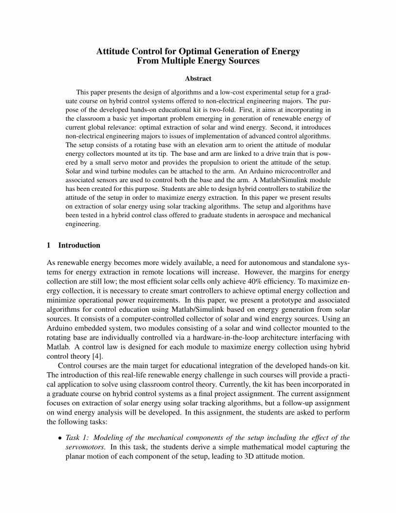
Before a hybrid control system is implemented, the reference position of the sun must be deter-mined. The resulting reference position will be the output of the reference generator for the hybridplant, in this case the solar collector, to track. The method used here will create a reference trajec-tory for the plant to track. The methods to create controllers for tracking and analyze stability areoutlined in [5]. To maximize solar energy input, the angle between the unit vector normal to theplane of the lens (nc) and the unit vector of the solar rays (ns) must be minimized. The parame-ters used to derive the solar vector are: local time t, hour angle ω, declination angle δ, and locallatitude λ. Hour and declination angle are calculated using (1) and (2), respectively. The solarposition calculations are outlined in [3] and [1]. The position angles of the solar cooker apparatus,azimuth φ and zenith β, are displayed in Fig. 2 and represent the position of the solar cooker arm

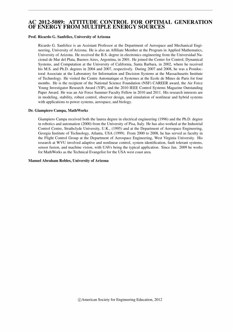
(a) Top view. (b) Side view.

Figure 1: (a) The azimuth angle is measured between the front normal vector and the South direc-tion. (b) The zenith angle is measured between the arm of the collector and the vertical axis.

with respect to the vertical and horizontal planes.

ω(t) = (360/24)t (1)

δ = 23.45 sin(360(284 + n)/365) (2)

The solar vector is found using (3) as a function of the solar parameters and the lens normal vectoris found as a function of the solar cooker angles.

ns = (cos δ cosω cosλ+ sin δ sinλ,− cos δ sinω,− cos δ cosω sinλ+ sin δ cosλ) (3)

nc = (cos β,− sin β sinφ,− sin β cosφ) (4)

Figure 2: Cartesian view of the solar vector ns and lens normal vector ns projected onto respectiveplanes.

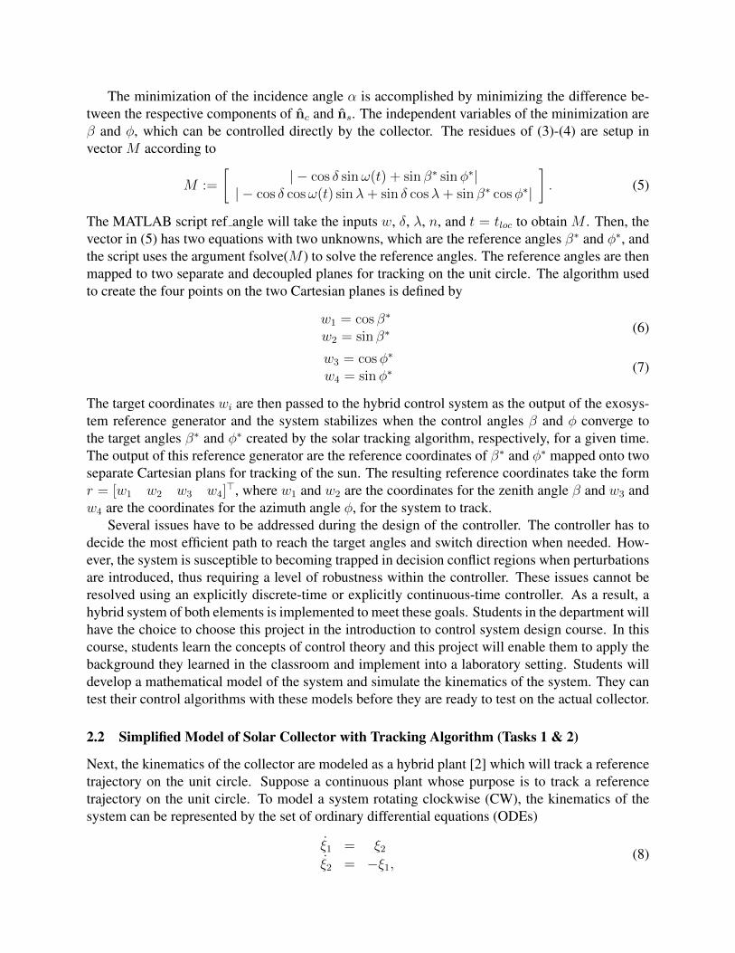
The minimization of the incidence angle α is accomplished by minimizing the difference be-tween the respective components of nc and ns. The independent variables of the minimization areβ and φ, which can be controlled directly by the collector. The residues of (3)-(4) are setup invector M according to

M :=

[| − cos δ sinω(t) + sin β∗ sinφ∗|

| − cos δ cosω(t) sinλ+ sin δ cosλ+ sin β∗ cosφ∗|

]. (5)

The MATLAB script ref angle will take the inputs w, δ, λ, n, and t = tloc to obtain M . Then, thevector in (5) has two equations with two unknowns, which are the reference angles β∗ and φ∗, andthe script uses the argument fsolve(M ) to solve the reference angles. The reference angles are thenmapped to two separate and decoupled planes for tracking on the unit circle. The algorithm usedto create the four points on the two Cartesian planes is defined by

w1 = cos β∗

w2 = sin β∗(6)

w3 = cosφ∗

w4 = sinφ∗(7)

The target coordinates wi are then passed to the hybrid control system as the output of the exosys-tem reference generator and the system stabilizes when the control angles β and φ converge tothe target angles β∗ and φ∗ created by the solar tracking algorithm, respectively, for a given time.The output of this reference generator are the reference coordinates of β∗ and φ∗ mapped onto twoseparate Cartesian plans for tracking of the sun. The resulting reference coordinates take the formr = [w1 w2 w3 w4]

>, where w1 and w2 are the coordinates for the zenith angle β and w3 andw4 are the coordinates for the azimuth angle φ, for the system to track.

Several issues have to be addressed during the design of the controller. The controller has todecide the most efficient path to reach the target angles and switch direction when needed. How-ever, the system is susceptible to becoming trapped in decision conflict regions when perturbationsare introduced, thus requiring a level of robustness within the controller. These issues cannot beresolved using an explicitly discrete-time or explicitly continuous-time controller. As a result, ahybrid system of both elements is implemented to meet these goals. Students in the department willhave the choice to choose this project in the introduction to control system design course. In thiscourse, students learn the concepts of control theory and this project will enable them to apply thebackground they learned in the classroom and implement into a laboratory setting. Students willdevelop a mathematical model of the system and simulate the kinematics of the system. They cantest their control algorithms with these models before they are ready to test on the actual collector.

2.2 Simplified Model of Solar Collector with Tracking Algorithm (Tasks 1 & 2)

Next, the kinematics of the collector are modeled as a hybrid plant [2] which will track a referencetrajectory on the unit circle. Suppose a continuous plant whose purpose is to track a referencetrajectory on the unit circle. To model a system rotating clockwise (CW), the kinematics of thesystem can be represented by the set of ordinary differential equations (ODEs)

ξ1 = ξ2ξ2 = −ξ1,

(8)

which will hold true as long as ξ1 and ξ2 remain on the unit circle.For an initial condition of ξ(0, 0) that is on the unit circle, the solution φp to these dynamics

will result in a signal CW rotating around the unit circle. To rotate around the unit circle counterclockwise (CCW), simply invert the signs of ξ1 and ξ2, and the resulting solution is a signal rotatingCCW on the unit circle. By introducing a scalar control input uc to the plant kinematics, the planttakes the form

ξ1 = ucξ2ξ2 = −ucξ1.

(9)

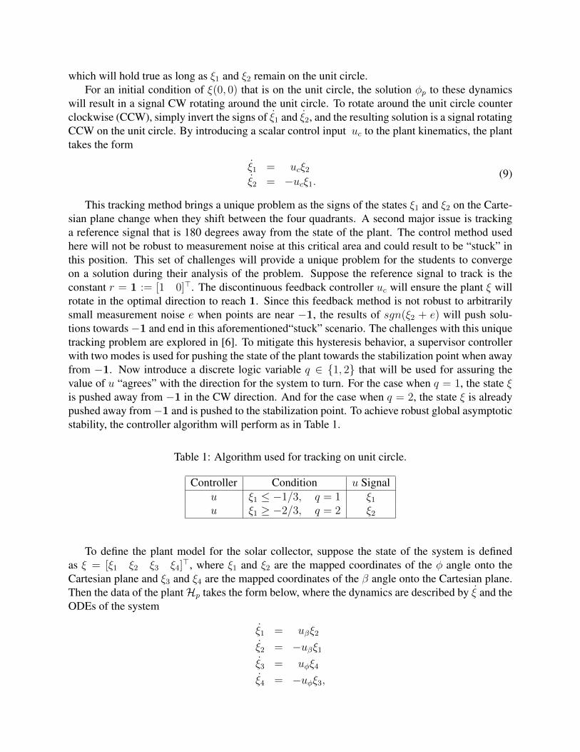
This tracking method brings a unique problem as the signs of the states ξ1 and ξ2 on the Carte-sian plane change when they shift between the four quadrants. A second major issue is trackinga reference signal that is 180 degrees away from the state of the plant. The control method usedhere will not be robust to measurement noise at this critical area and could result to be “stuck” inthis position. This set of challenges will provide a unique problem for the students to convergeon a solution during their analysis of the problem. Suppose the reference signal to track is theconstant r = 1 := [1 0]>. The discontinuous feedback controller uc will ensure the plant ξ willrotate in the optimal direction to reach 1. Since this feedback method is not robust to arbitrarilysmall measurement noise e when points are near −1, the results of sgn(ξ2 + e) will push solu-tions towards−1 and end in this aforementioned“stuck” scenario. The challenges with this uniquetracking problem are explored in [6]. To mitigate this hysteresis behavior, a supervisor controllerwith two modes is used for pushing the state of the plant towards the stabilization point when awayfrom −1. Now introduce a discrete logic variable q ∈ {1, 2} that will be used for assuring thevalue of u “agrees” with the direction for the system to turn. For the case when q = 1, the state ξis pushed away from −1 in the CW direction. And for the case when q = 2, the state ξ is alreadypushed away from−1 and is pushed to the stabilization point. To achieve robust global asymptoticstability, the controller algorithm will perform as in Table 1.

Table 1: Algorithm used for tracking on unit circle.

Controller Condition u Signalu ξ1 ≤ −1/3, q = 1 ξ1u ξ1 ≥ −2/3, q = 2 ξ2

To define the plant model for the solar collector, suppose the state of the system is definedas ξ = [ξ1 ξ2 ξ3 ξ4]

>, where ξ1 and ξ2 are the mapped coordinates of the φ angle onto theCartesian plane and ξ3 and ξ4 are the mapped coordinates of the β angle onto the Cartesian plane.Then the data of the plantHp takes the form below, where the dynamics are described by ξ and theODEs of the system

ξ1 = uβξ2

ξ2 = −uβξ1ξ3 = uφξ4

ξ4 = −uφξ3,

where the points (ξ1, ξ2) and (ξ3, ξ4) are on the unit circle. An additional q variable is added andare labeled as q1 and q2 for each degree of freedom.

To track the signals (6)-(7) from the exosystem, the attitude of the apparatus is stabilized to theposition of the sun such that (ξ1, ξ2) = (w1, w2) and (ξ3, ξ4) = (w3, w4). To achieve this on theunit circle, a coordinate transformation method used. Using the transformation[

z1z2

]=

[ξ1w1 − ξ2w2

w2ξ1 + w1ξ2

], (10)

[z3z4

]=

[ξ3w3 − ξ4w4

w4ξ3 + w3ξ4

], (11)

the new dynamics of the plant take the form

z1 = uβz2z2 = −uβz1z3 = uφz4z4 = −uφz3,

(12)

where uβ and uφ are the new control inputs for each degree of freedom. Now for when (ξ1, ξ2) =(w1, w2) ⇐⇒ (z1, z2) = (1, 0) and (ξ3, ξ4) = (w3, w4) ⇐⇒ (z3, z4) = (1, 0). Thus, the state ofthe original plant ξ will stabilize to w.

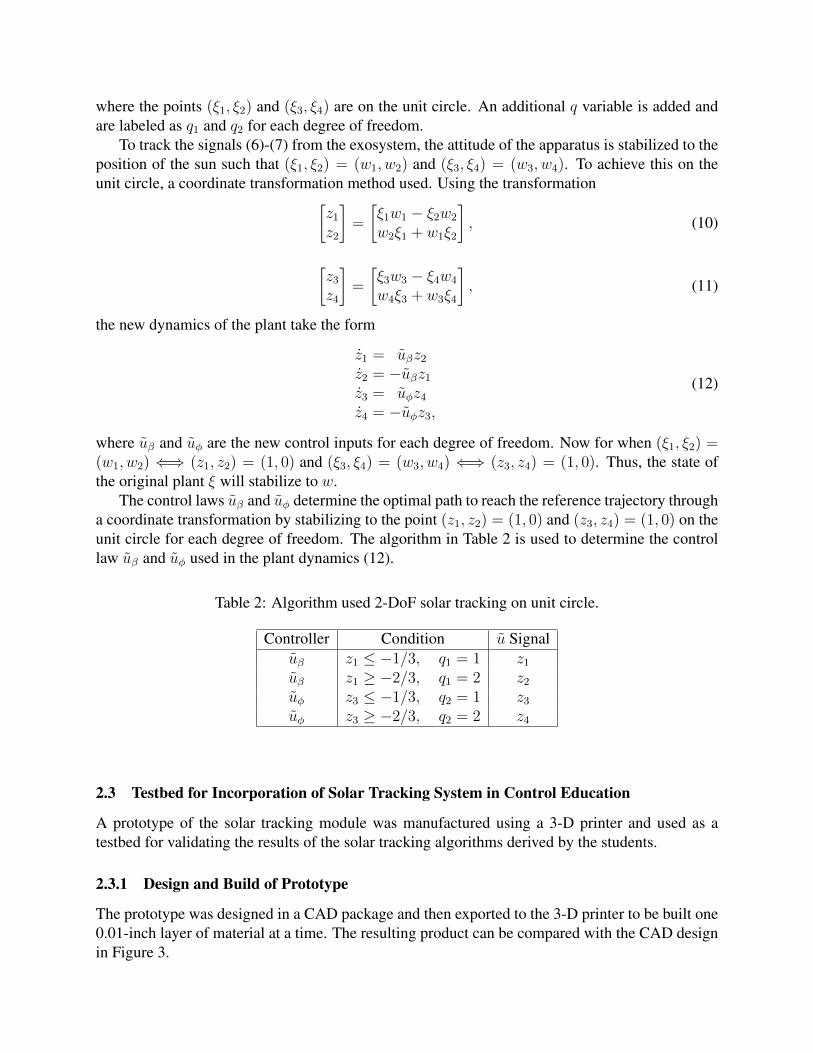
The control laws uβ and uφ determine the optimal path to reach the reference trajectory througha coordinate transformation by stabilizing to the point (z1, z2) = (1, 0) and (z3, z4) = (1, 0) on theunit circle for each degree of freedom. The algorithm in Table 2 is used to determine the controllaw uβ and uφ used in the plant dynamics (12).

Table 2: Algorithm used 2-DoF solar tracking on unit circle.

Controller Condition u Signaluβ z1 ≤ −1/3, q1 = 1 z1uβ z1 ≥ −2/3, q1 = 2 z2uφ z3 ≤ −1/3, q2 = 1 z3uφ z3 ≥ −2/3, q2 = 2 z4

2.3 Testbed for Incorporation of Solar Tracking System in Control Education

A prototype of the solar tracking module was manufactured using a 3-D printer and used as atestbed for validating the results of the solar tracking algorithms derived by the students.

2.3.1 Design and Build of Prototype

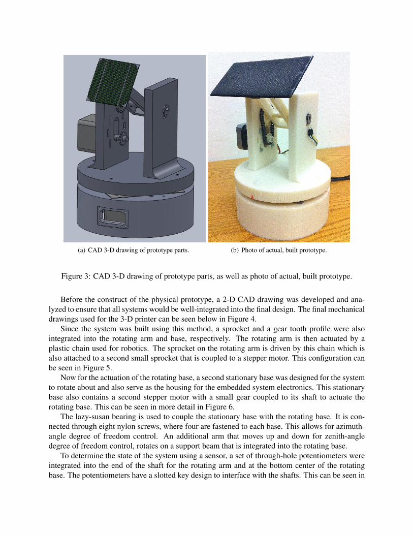
The prototype was designed in a CAD package and then exported to the 3-D printer to be built one0.01-inch layer of material at a time. The resulting product can be compared with the CAD designin Figure 3.

(a) CAD 3-D drawing of prototype parts. (b) Photo of actual, built prototype.

Figure 3: CAD 3-D drawing of prototype parts, as well as photo of actual, built prototype.

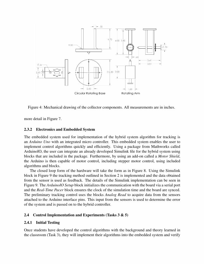
Before the construct of the physical prototype, a 2-D CAD drawing was developed and ana-lyzed to ensure that all systems would be well-integrated into the final design. The final mechanicaldrawings used for the 3-D printer can be seen below in Figure 4.

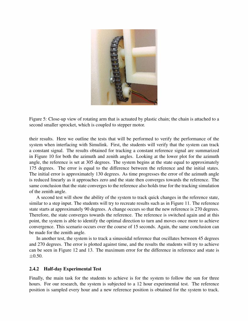
Since the system was built using this method, a sprocket and a gear tooth profile were alsointegrated into the rotating arm and base, respectively. The rotating arm is then actuated by aplastic chain used for robotics. The sprocket on the rotating arm is driven by this chain which isalso attached to a second small sprocket that is coupled to a stepper motor. This configuration canbe seen in Figure 5.

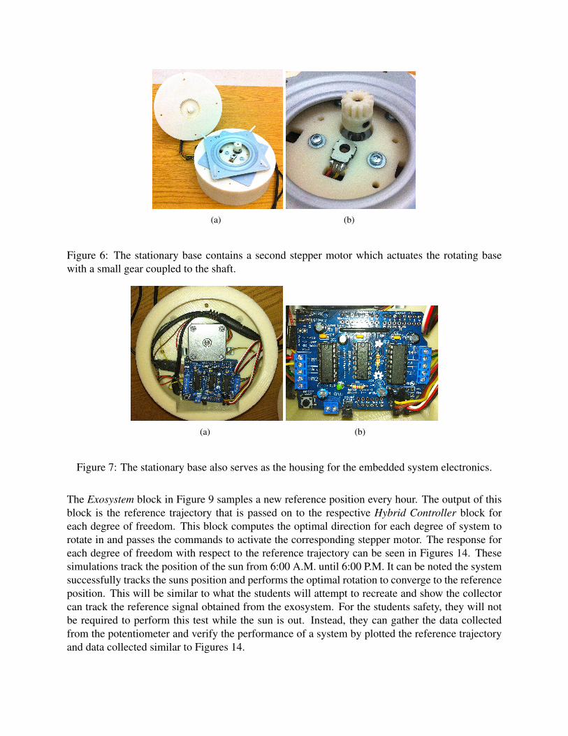
Now for the actuation of the rotating base, a second stationary base was designed for the systemto rotate about and also serve as the housing for the embedded system electronics. This stationarybase also contains a second stepper motor with a small gear coupled to its shaft to actuate therotating base. This can be seen in more detail in Figure 6.

The lazy-susan bearing is used to couple the stationary base with the rotating base. It is con-nected through eight nylon screws, where four are fastened to each base. This allows for azimuth-angle degree of freedom control. An additional arm that moves up and down for zenith-angledegree of freedom control, rotates on a support beam that is integrated into the rotating base.

To determine the state of the system using a sensor, a set of through-hole potentiometers wereintegrated into the end of the shaft for the rotating arm and at the bottom center of the rotatingbase. The potentiometers have a slotted key design to interface with the shafts. This can be seen in

Figure 4: Mechanical drawing of the collector components. All measurements are in inches.

more detail in Figure 7.

2.3.2 Electronics and Embedded System

The embedded system used for implementation of the hybrid system algorithm for tracking isan Arduino Uno with an integrated micro controller. This embedded system enables the user toimplement control algorithms quickly and efficiently. Using a package from Mathworks calledArduinoIO, the user can integrate an already developed Simulink file for the hybrid system usingblocks that are included in the package. Furthermore, by using an add-on called a Motor Shield,the Arduino is then capable of motor control, including stepper motor control, using includedalgorithms and blocks.

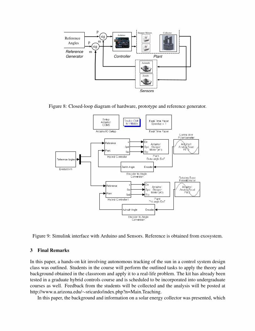
The closed loop form of the hardware will take the form as in Figure 8. Using the Simulinkblock in Figure 9 the tracking method outlined in Section 2 is implemented and the data obtainedfrom the sensor is used as feedback. The details of the Simulink implementation can be seen inFigure 9. The ArduinoIO Setup block initializes the communication with the board via a serial portand the Real-Time Pacer block ensures the clock of the simulation time and the board are synced.The preliminary tracking control uses the blocks Analog Read to acquire data from the sensorsattached to the Arduino interface pins. This input from the sensors is used to determine the errorof the system and is passed on to the hybrid controller.

2.4 Control Implementation and Experiments (Tasks 3 & 5)

2.4.1 Initial Testing

Once students have developed the control algorithms with the background and theory learned inthe classroom (Task 3), they will implement their algorithms into the embedded system and verify

Figure 5: Close-up view of rotating arm that is actuated by plastic chain; the chain is attached to asecond smaller sprocket, which is coupled to stepper motor.

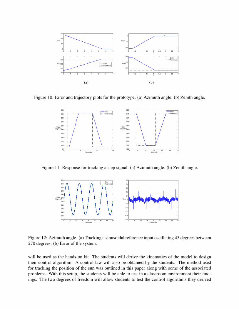
their results. Here we outline the tests that will be performed to verify the performance of thesystem when interfacing with Simulink. First, the students will verify that the system can tracka constant signal. The results obtained for tracking a constant reference signal are summarizedin Figure 10 for both the azimuth and zenith angles. Looking at the lower plot for the azimuthangle, the reference is set at 305 degrees. The system begins at the state equal to approximately175 degrees. The error is equal to the difference between the reference and the initial states.The initial error is approximately 130 degrees. As time progresses the error of the azimuth angleis reduced linearly as it approaches zero and the state then converges towards the reference. Thesame conclusion that the state converges to the reference also holds true for the tracking simulationof the zenith angle.

A second test will show the ability of the system to track quick changes in the reference state,similar to a step input. The students will try to recreate results such as in Figure 11. The referencestate starts at approximately 90 degrees. A change occurs so that the new reference is 270 degrees.Therefore, the state converges towards the reference. The reference is switched again and at thispoint, the system is able to identify the optimal direction to turn and moves once more to achieveconvergence. This scenario occurs over the course of 15 seconds. Again, the same conclusion canbe made for the zenith angle.

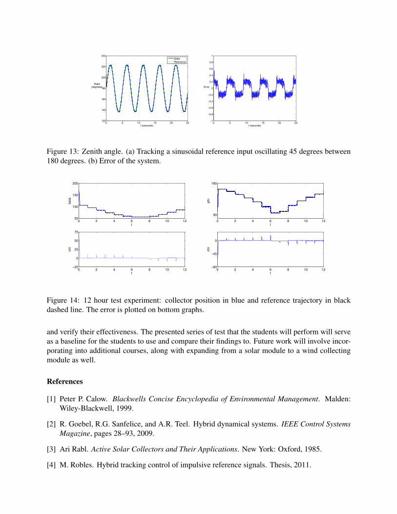
In another test, the system is to track a sinusoidal reference that oscillates between 45 degreesand 270 degrees. The error is plotted against time, and the results the students will try to achievecan be seen in Figure 12 and 13. The maximum error for the difference in reference and state is±0.50.

2.4.2 Half-day Experimental Test

Finally, the main task for the students to achieve is for the system to follow the sun for threehours. For our research, the system is subjected to a 12 hour experimental test. The referenceposition is sampled every hour and a new reference position is obtained for the system to track.

(a) (b)

Figure 6: The stationary base contains a second stepper motor which actuates the rotating basewith a small gear coupled to the shaft.

(a) (b)

Figure 7: The stationary base also serves as the housing for the embedded system electronics.

The Exosystem block in Figure 9 samples a new reference position every hour. The output of thisblock is the reference trajectory that is passed on to the respective Hybrid Controller block foreach degree of freedom. This block computes the optimal direction for each degree of system torotate in and passes the commands to activate the corresponding stepper motor. The response foreach degree of freedom with respect to the reference trajectory can be seen in Figures 14. Thesesimulations track the position of the sun from 6:00 A.M. until 6:00 P.M. It can be noted the systemsuccessfully tracks the suns position and performs the optimal rotation to converge to the referenceposition. This will be similar to what the students will attempt to recreate and show the collectorcan track the reference signal obtained from the exosystem. For the students safety, they will notbe required to perform this test while the sun is out. Instead, they can gather the data collectedfrom the potentiometer and verify the performance of a system by plotted the reference trajectoryand data collected similar to Figures 14.

Controller

ArduinoStepper Motors

Plant

Collector

Azimuth

Sensors

Zenith

sig

sig

m

m

p

p

Reference

Angles

Reference

Generator

Figure 8: Closed-loop diagram of hardware, prototype and reference generator.

Figure 9: Simulink interface with Arduino and Sensors. Reference is obtained from exosystem.

3 Final Remarks

In this paper, a hands-on kit involving autonomous tracking of the sun in a control system designclass was outlined. Students in the course will perform the outlined tasks to apply the theory andbackground obtained in the classroom and apply it to a real-life problem. The kit has already beentested in a graduate hybrid controls course and is scheduled to be incorporated into undergraduatecourses as well. Feedback from the students will be collected and the analysis will be posted athttp://www.u.arizona.edu/∼sricardo/index.php?n=Main.Teaching.

In this paper, the background and information on a solar energy collector was presented, which

0 1 2 3 4 5 6 7

0

50

100

150

t

Error

0 1 2 3 4 5 6 7150

200

250

300

t

State

State

Reference

(a)

0 0.5 1 1.5 2 2.5 3 3.5 4

−100

−50

0

t

Error

0 0.5 1 1.5 2 2.5 3 3.5 4

200

250

300

t

State

State

Reference

(b)

Figure 10: Error and trajectory plots for the prototype. (a) Azimuth angle. (b) Zenith angle.

0 5 10 1580

100

120

140

160

180

200

220

240

260

280

State (degrees)

t (seconds)

State

Reference

0 5 10 15 20 25 30160

180

200

220

240

260

280

300

320

340

360

State (degrees)

t (seconds)

State

Reference

Figure 11: Response for tracking a step signal. (a) Azimuth angle. (b) Zenith angle.

0 5 10 15 20 25 30 35 40210

220

230

240

250

260

270

280

290

300

310

320

State (degrees)

t (seconds)

State

Reference

0 5 10 15 20 25 30 35 40−0.5

−0.4

−0.3

−0.2

−0.1

0

0.1

0.2

0.3

0.4

0.5

Error

t (seconds)

Figure 12: Azimuth angle. (a) Tracking a sinusoidal reference input oscillating 45 degrees between270 degrees. (b) Error of the system.

will be used as the hands-on kit. The students will derive the kinematics of the model to designtheir control algorithm. A control law will also be obtained by the students. The method usedfor tracking the position of the sun was outlined in this paper along with some of the associatedproblems. With this setup, the students will be able to test in a classroom environment their find-ings. The two degrees of freedom will allow students to test the control algorithms they derived

0 5 10 15 20 25120

140

160

180

200

220

240

State (degrees)

t (seconds)

State

Reference

0 5 10 15 20 25−1

−0.8

−0.6

−0.4

−0.2

0

0.2

0.4

0.6

0.8

1

Error

t (seconds)

Figure 13: Zenith angle. (a) Tracking a sinusoidal reference input oscillating 45 degrees between180 degrees. (b) Error of the system.

0 2 4 6 8 10 1250

100

150

200

be

ta

t

0 2 4 6 8 10 12−25

0

25

50

75

chi

t

0 2 4 6 8 10 12

90

180

phi

t

0 2 4 6 8 10 12−90

−45

0

chi

t

Figure 14: 12 hour test experiment: collector position in blue and reference trajectory in blackdashed line. The error is plotted on bottom graphs.

and verify their effectiveness. The presented series of test that the students will perform will serveas a baseline for the students to use and compare their findings to. Future work will involve incor-porating into additional courses, along with expanding from a solar module to a wind collectingmodule as well.

References

[1] Peter P. Calow. Blackwells Concise Encyclopedia of Environmental Management. Malden:Wiley-Blackwell, 1999.

[2] R. Goebel, R.G. Sanfelice, and A.R. Teel. Hybrid dynamical systems. IEEE Control SystemsMagazine, pages 28–93, 2009.

[3] Ari Rabl. Active Solar Collectors and Their Applications. New York: Oxford, 1985.

[4] M. Robles. Hybrid tracking control of impulsive reference signals. Thesis, 2011.

[5] M. Robles and R. G. Sanfelice. Hybrid controllers for tracking of impulsive reference trajec-tories: A hybrid exosystem approach. In Proc. 14th International Conference Hybrid Systems:Control and Computation, pages 231–240, 2011.

[6] R. G. Sanfelice, A. R. Teel, and R. Goebel. Supervising a family of hybrid controllers for ro-bust global asymptotic stabilization. In Proc. 47th IEEE Conference on Decision and Control,pages 4700–4705, 2008.