Attitude Tracking Control Simulating the HubbleSpace Telescope

Brett Streetman

December 12, 2003

Contents

1 Introduction and Background 11.1 Hubble Space Telescope . . . . . . . . . . . . . . . . . . . . . . . . . 1

1.1.1 Pointing Control System Operations . . . . . . . . . . . . . . 21.2 Attitude Tracking Control . . . . . . . . . . . . . . . . . . . . . . . . 3

2 Problem Statement and Equations of Motion 4

3 Analysis 63.1 Reference Motion . . . . . . . . . . . . . . . . . . . . . . . . . . . . . 63.2 PID Controller . . . . . . . . . . . . . . . . . . . . . . . . . . . . . . 7

3.2.1 Initial Gain Selection . . . . . . . . . . . . . . . . . . . . . . . 8

4 Results 104.1 Linear and Nonlinear Equations . . . . . . . . . . . . . . . . . . . . . 104.2 Static Gains . . . . . . . . . . . . . . . . . . . . . . . . . . . . . . . . 114.3 Gain Scheduling . . . . . . . . . . . . . . . . . . . . . . . . . . . . . . 124.4 Continuous State-Dependent Gains . . . . . . . . . . . . . . . . . . . 144.5 Conclusion . . . . . . . . . . . . . . . . . . . . . . . . . . . . . . . . . 16

i

Chapter 1

Introduction and Background

The Hubble Space Telescope (HST) was launched April 24, 1990 in the shuttleDiscovery. The HST was named after American astronomer Edwin Hubble, madefamous for his discovery of the constant expansion of the universe. The telescopebearing his name has made some of the most important astronomical observations ofthe modern era. The Hubble was design for versatility and longevity. It has performmany diverse missions, including documenting the structure of the Solar System,searching for planets in other solar systems, and attempting to discover the size andnature of the entire Universe.

To take scientifically useful photos, the attitude control of the Hubble must bestringent. The design criteria are for it to be able to track an inertially fixed targetwith error of no more than 0.007 arcseconds for anywhere from 10 minutes to 24hours[1]. The accuracy involved is equivalent to hitting a dime with laser from 322kilometers away and never straying past the edge of the coin.

1.1 Hubble Space Telescope

Plans for the eventual space telescope began at NASA in the early 1970’s. Orig-inally, the telescope was supposed to have a 3 meter aperture, but that was laterrelaxed to 2.4 meters[2]. The size reduction went hand in hand with other specifica-tion relaxations to reduce the cost of the project in a 1974 redesign. In 1976, Glaese,et al.[2] presented a Pointing Control System (PCS) that much resembles the systemused on the Hubble. Dougherty, et al.[3] produced a more detailed document on thePCS hardware in 1982. The proposed testing procedure for the PCS was outlined inthis paper, and called for the construction of a spherical air bearing tabletop simulatorto test the fine pointing scheme.

After the Hubble was launched, vibrations in the solar panels caused the PointingControl System (PCS) to not perform up to specifications. In 1995, NASA scientistsFoster, et al.[4] described the nature of these vibrations. The excitations were ascribedto thermal deformations of the solar panels. The vibrations were more intense than

1

CHAPTER 1. INTRODUCTION AND BACKGROUND 2

predicted by the attitude system designers and the PCS could not overcome them.The initial controller was redesigned and uploaded to the Hubble, but NASA tookadvantage of the large amount of data collected to solve the problem and commis-sioned five different organizations to develop their own controller for HST. Addingtonand Johnson[5] at the University of Alabama developed a dual-mode disturbance-accommodating controller that both provides torques to counteract disturbances andtorques to augment the natural damping of the solar arrays. Collins and Richter[6]at Florida A&M University created a linear quadratic Gaussian design for the PCS.An H∞ controller was both analytically and numerically derived by Irwin, et al.[7] atOhio University. Zhu, et al.[8] developed a controller for the Hubble based on covari-ance control techniques. Nurre, et al.[9] from NASA’s Marshall Spaceflight Centerdescribed the evolution of the SAGA-II controller. The SAGA-II was an extension ofthe original controller on the Hubble, designed to account for solar array vibrations.On April 16, 1992, the SAGA-II controller became the normal operating mode forthe Hubble, and succeeded in reducing the effect of the vibrations to an acceptablelevel.

In addition to its initial attitude problems, Hubble had an aberration on one ofits mirrors that caused low picture quality. A corrective optics unit was installed onthe telescope during its first servicing mission. The Hubble could begin its sciencework in earnest now.

With its initial problems fixed, the Hubble began to take photographs that metand exceeded original expectations. In 1996, Fischer and Duerbeck[10] publisheda book displaying a large number of these photos. Along with the large numberof photographs, the book contained a full description of Hubble’s systems and anoverview of the science missions being pursued by the HST.

The official NASA HST website[1] has the most current information on the Hubble.This includes specifications, subsystem descriptions, service timelines, and missionobjectives. Much information, current or historical, can be found on this website. Asecond website with more technical information is located at Ref. [11].

1.1.1 Pointing Control System Operations

Pointing Control System operation begins with coarse attitude determination.The HST contains a sun sensor and magnetometer to get a first approximation of itsorientation. The Fixed Head Star Trackers then search the starfield for recognizedpatterns to gain more exact attitude knowledge. The Hubble is reoriented by the useof four reaction wheels. The HST contains six rate gyros. Three of these are operatingat any given time to determine the angular velocities of the telescope. When theHubble has acquired its target using the ”coarse” guidance of the Fixed Head StarTrackers, the fine guidance system takes control. The Fine Guidance Sensors (FGS)are used to gain a near exact lock on a target. There are three FGSs on the Hubble.Two lock onto individual stars around the target, while the third focuses itself and

CHAPTER 1. INTRODUCTION AND BACKGROUND 3

the optics onto the target itself. The two FGSs not on the target keep their individualstar inside of a fixed area in their field of view, using the information from the rategyros and controlling with the reaction wheels.

1.2 Attitude Tracking Control

Pointing HST at an astronomical target involves the Hubble tracking that objectfor a certain period of time. Most of Hubble’s target are many light years away, so theycan be considered fixed in the inertial reference frame. Hablani[12] has has performeda large amount of work in this area, extending many principles to the tracking ofnon-inertially fixed targets. Hall[13] has also worked with attitude tracking and hasdeveloped a tracking controller using momentum wheels and thrusters.

Chapter 2

Problem Statement and Equationsof Motion

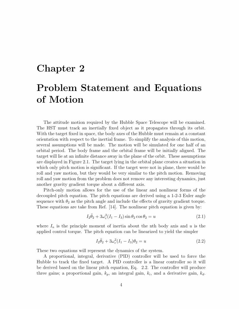
The attitude motion required by the Hubble Space Telescope will be examined.The HST must track an inertially fixed object as it propagates through its orbit.With the target fixed in space, the body axes of the Hubble must remain at a constantorientation with respect to the inertial frame. To simplify the analysis of this motion,several assumptions will be made. The motion will be simulated for one half of anorbital period. The body frame and the orbital frame will be initially aligned. Thetarget will lie at an infinite distance away in the plane of the orbit. These assumptionsare displayed in Figure 2.1. The target lying in the orbital plane creates a situation inwhich only pitch motion is significant. If the target were not in plane, there would beroll and yaw motion, but they would be very similar to the pitch motion. Removingroll and yaw motion from the problem does not remove any interesting dynamics, justanother gravity gradient torque about a different axis.

Pitch-only motion allows for the use of the linear and nonlinear forms of thedecoupled pitch equation. The pitch equations are derived using a 1-2-3 Euler anglesequence with θ2 as the pitch angle and include the effects of gravity gradient torque.These equations are take from Ref. [14]. The nonlinear pitch equation is given by:

I2θ2 + 3ω2c (I1 − I3) sin θ2 cos θ2 = u (2.1)

where In is the principle moment of inertia about the nth body axis and u is theapplied control torque. The pitch equation can be linearized to yield the simpler

I2θ2 + 3ω2c (I1 − I3)θ2 = u (2.2)

These two equations will represent the dynamics of the system.A proportional, integral, derivative (PID) controller will be used to force the

Hubble to track the fixed target. A PID controller is a linear controller so it willbe derived based on the linear pitch equation, Eq. 2.2. The controller will producethree gains; a proportional gain, kp, an integral gain, ki, and a derivative gain, kd.

4

CHAPTER 2. PROBLEM STATEMENT AND EQUATIONS OF MOTION 5

Figure 2.1: Attitude motion to be simulated

These three gains will be tuned to work with the actual reaction wheel hardware onHST. The gains will be tuned in three different ways: a static gain case, a scheduledgain case, and a continuous state-dependent gain case.

Chapter 3

Analysis

3.1 Reference Motion

The desired motion of the Hubble can be described by a virtual spacecraft thatperfectly tracks the target. The controller will then try to match this motion throughtime. The desired motion will be defined by a desired pitch angle, θd. The controlleroperates by minimizing the error between θd and θ2.

The first step in determining the reference motion is to determine Hubble’s orbit.A recent two line element set (TLE) for HST was obtained from Ref. [15]. TheTLE was analyzed to calculate the orbital elements of the orbit. Using the orbitalelements, the rotation matrix between the orbital frame and the inertial frame, Roi,can be calculated by an equation from Ref. [14]:

Roi =

−su cΩ − cu ci sΩ −su sΩ + cu ci cΩ cu si−si sΩ si cΩ −ci−cu cΩ + su ci sΩ −cu sΩ − su ci cΩ −su si

(3.1)

where s or c denotes sin or cos of an angle, and i is the inclination, Ω is the rightascension of the ascending node, and u is the argument of latitude. Based on theassumptions made for this problem, the orbital frame and the body frame are initiallyaligned, so

Rbi = Roi|t=0 (3.2)

The body frame is constant with respect with to the inertial frame so this Rbi is validfor all time.

A forward propagation of the orbital elements can then be performed. The prop-agation was performed using a Matlab code obtained from Ref. [14]. The time stepchosen for this propagation was 0.5 seconds. After each step forward, a new set of or-bital elements was plugged into Eq. 3.1. The new Roi was used with Rbi to calculatethe rotation between the body frame and the orbital, Rbo, by:

Rbo = Rbi(Roi)T (3.3)

6

CHAPTER 3. ANALYSIS 7

The orbital to body rotation matrix for a 1-2-3 Euler angle sequence takes the fol-lowing form[14]:

Rbo =

c2c3 s1s2c3 + c1s3 s1s3 − c1s2c3

−s2s3 c1c3 − s1s2s3 s1c3 + c1s2s3

s2 −s1c2 c1c2

(3.4)

where sn and cn represents the sin or cos of θn. The (3,1) element of the Rbo matrixdepends only on the pitch angle. The desired pitch angle, θd can be easily solved forby:

θd = sin−1(Rbo(3, 1)) (3.5)

The correct quadrant of θd can be found by combining other terms of Rbo to getanother expression for the pitch angle. The resulting virtual satellite reference motionis presented in Fig. 3.1. As can be easily seen in the figure, θd increases linearly withtime. Fitting a line to this data yields the result of

θd =2π

Tp

t (3.6)

where Tp is the period of Hubble’s orbit. The linear nature of this result removesseveral difficulties in control that arise in a reference motion that is nonlinear and notknown as a discrete function of time.

3.2 PID Controller

A proportional, integral, derivative (PID) controller is a simple type of linear con-troller. A PID controller is not complicated to derive and not difficult to implement.The interesting part of PID control comes in the selection of its three gains: theproportional gain, kp, the integral gain, ki, and the derivative gain kd.

A PID controller assumes a control of the form

u = −kpx − ki

∫ t

0x(τ)dτ − kdx (3.7)

where x is the state that is to be controlled. In this problem, the pitch angle of theactual spacecraft is supposed to be tracking the desired pitch angle of the virtualspacecraft. The state to be controlled then is defined as δθ, which is given by

δθ = θd − θ2 (3.8)

where θ2 is the pitch angle of the actual spacecraft. The PID control term can nowbe written as

u = −kpδθ − ki

∫ t

0δθdτ − kdδθ (3.9)

CHAPTER 3. ANALYSIS 8

Figure 3.1: Reference motion pitch angle

The integral and derivative of θd can easily be calculated from Eq. 3.6 and the valuesfor θ2 are part of the states and must be integrated with the equations of motion.The linear equation of motion now becomes

I2θ2 + 3ω2c (I1 − I3)θ2 + kpδθ + ki

∫ t

0δθdτ + kdδθ = 0 (3.10)

A PID controller can easily be shown to be a stable controller by forming the Laplacetransform characteristic equation and applying the Final Value Theorem to it.

The PID controller is applied to the nonlinear equation of motion by simply in-serting the control torque expression of Eq. 3.9 into the nonlinear pitch equation.

3.2.1 Initial Gain Selection

An initial guess at the proper gains can be found by factoring the characteristicequation of the system in terms of three new variables: the natural frequency, ωn, thedamping ratio, ζ, and the integral time constant, T . The gains are classically definedby these terms as[14]:

kp0 = ω2n +

2ζωn

T− ko (3.11)

CHAPTER 3. ANALYSIS 9

ki0 =ω2

n

T(3.12)

kd0 = 2ζωn +1

T(3.13)

where the zero subscript on the gains is the notation used to reference these baseguesses. In this problem, the three independent variable were defined as follows

ωn =(3ω2

c

I2 − I1

I3

) 12

(3.14)

ζ = 0.7 (3.15)

T =10

ζωn

(3.16)

where ωc is the mean motion of Hubble’s orbit. These values are completely arbitraryand are only used as a starting point for tuning the gains. However, starting withreasonable values in the above equations can usually give gains within one or twoorders of magnitude of the proper ones.

Chapter 4

Results

The PID controller presented in the last chapter was applied to a variety of caseswith both the linear and nonlinear equations of motions in a Matlab simulation. Thegains were also tuned in a variety of ways. First, a single set of gains was used forthe entire length of the simulation. Next, the method of gain scheduling was applied.Gain scheduling involves the use of two or more discrete sets of gains, dependingon whether the error is large or small. The third method applied is referred to ascontinuous state-dependent gains (CSDG). Implementing a CSDG controller involveschoosing the gains as a continuous function of the states.

In an effort to make the simulations more realistic a maximum control toque valuewas implemented. The maximum torque HST could apply to any control axis wasestimated at 1.6 N-m. Although this value is much larger than most satellites wouldhave, the 2-axis moment of inertia for the Hubble is 77,217 kg-m2[9], requiring quitea large torque to get it moving. Any time a controller asked for a torque that wastoo large it was only allowed to apply a torque 80% of the maximum value. Themaximum angular velocity of the simulated HST was also limited. The real Hubblehas a maximum slew rate of 0.00175 rad/s, or about the rate of the minute handon a clock. In simulation, this maximum angular velocity was assumed to be whenthe reaction wheels had reached their maximum spin rate. If the wheel is alreadyat its maximum speed, no further control torque can be applied. This situation wasmodeled by having the wheels apply a small torque in the opposite direction if themaximum angular velocity was reached.

4.1 Linear and Nonlinear Equations

A Matlab simulation was developed for both the linear and nonlinear equations ofmotion. These simulations were run for a variety of initial conditions and gains. Allof the trials show one result: the linear and nonlinear equations produce extremelysimilar results. This results holds even for for clearly non-small angle initial con-ditions. Figure 4.1 shows the results of the linear and nonlinear simulations for an

10

CHAPTER 4. RESULTS 11

initial pitch angle of 90 and an initial angular velocity of −0.0005 rad/s. The refer-ence motion starting conditions are 0 pitch angle and 0.0011 rad/s angular velocity.The two simulations produce results that are virtually indistinguishable. The twodifferent equations agreed similarly in every trial run. For this reason, all subsequentwork was performed only on the linear equation of motion.

Figure 4.1: Comparison of linear and nonlinear results

4.2 Static Gains

The use of static gains is the simplest form of PID control. One set of gains ischosen at the beginning of the simulation, and that set of gains is used no matterwhat the states are. The gains can then be tuned in order to find the best control.In this study, the best control was defined by the fastest acquisition of the referencemotion with a little overshoot as possible and the reaction wheels not reaching theirmaximum speed.

The first gains to try have been previously defined as kp0 , ki0 , and kd0 . Whenthese gains were applied, the system was slow to respond and sometimes unable toovercome the initial error before the end of the simulation. An increase in the gainswas in order. First, the proportional gain was increased by adding a multiplier to kp0

CHAPTER 4. RESULTS 12

until the system easily acquired the desired state. Then the integral gain was increasedto facilitate a faster reduction of error. The derivative gain can then be increased toeliminate or reduce any overshoot and overly large controls introduced by the previousgain increases. This process, of course, must be iterated many times, as changing onegain changes the relative behavior of the others. The eventual optimal gain set willhave the proportional and integral gains as large as possible and the derivative gainas small as possible, while still staying within the system constraints.

The constraints for this system were the maximum torque able to be applied andthe maximum wheel speed, which is defined by maximum angular velocity. The torqueconstraint was internally applied. If a controller asked for more than the maximumtorque, only the maximum value was given. If the maximum angular velocity wasreached a counter-torque was applied. However, the the tuning was performed sothat this never occurred. The gains for all three selection techniques were tuned for areference set of initial conditions, namely a 30 pitch angle error and an initial angularvelocity of -0.0005 rad/s. The gains were defined in terms of a multiplier on the basegains. For the static gain case best set of gains found was defined by:

kp = 75kp0 (4.1)

ki = 50ki0 (4.2)

kd = 20kd0 (4.3)

The result of applying these gains is presented in Fig. 4.2. The top plot shows thepitch angle of the actual spacecraft approaching the reference motion. The middleplot is of the pitch rate of the the actual craft. This quantity is the same as theangular velocity of the craft for the planar motion in the simulation. The bottomplot shows the control torque output by the controller as a function of time. Thecontrol for this case spends a short time at the minimum value before increasingrapidly, then beginning a steady decent to produce the steady reference motion. Theangular velocity decreases until it just flirts with the maximum value, and then itquickly approaches the reference value. The pitch angle error rapidly decreases untilreaching its desired valued with little to no overshoot.

4.3 Gain Scheduling

Gain scheduling (GS) is the next step up from static gain selection. To implementGS, multiple sets of static gains are chosen and implemented in different situations.At a minimum two set of gains are chosen, one for large errors and one for smallerrors. This simple implementation is what is pursued here. One set of gains wasused for errors larger than half of the initial error and one set was used for errors lessthan half of the initial error.

Gain scheduling is an improvement over static gains because the gains can be bet-ter tailored to individual situations. When the error is large, the integral gain should

CHAPTER 4. RESULTS 13

Figure 4.2: Best gain behavior for a set of static gains

be larger and the derivative gain smaller to quickly make up ground. When the erroris small, the integral gain should be smaller and the derivative gain larger to reduceovershoot. In the equation of motion, the control output by the proportional controlis already changing with the state, so it can usually remain constant throughout.

The two sets of gains chosen in this study were tuned to cover the error morequickly than the static gain case and still not overshoot. The best set of gains foundis presented in Table 4.1. The results produced by these sets of gains are shown

Table 4.1: Best gains found by the gain scheduling methodLarge δθ Small δθ

kp 75kp0 75kp0

ki 54ki0 44ki0

kd 18kd0 20kd0

in Fig. 4.3. The pitch angle data once again shows a fast, well-behaved controller.However, the GS controller reaches the reference motion 20 to 30 seconds earlier thanthe static controller. This improvement in speed comes at a price though. The controltorque switches quickly from its minimum to its maximum value. This change is more

CHAPTER 4. RESULTS 14

abrupt than seen in the static gain case and may be detrimental to a real motor. Theangular velocity of the spacecraft reaches its proper value slightly faster in the GScase, but also spends more time near its maximum value. Overall, the gain schedulingcontroller works faster but at a higher cost.

Figure 4.3: Best gain behavior for a set of scheduled gains

4.4 Continuous State-Dependent Gains

The use of continuous state-dependent gains (CSDG) takes gain scheduling to thenext level. The gains are defined by a continuous function of the state,amounting toan infinite number of GS sets. The gains can then be completely and easily tailoredto any situation that the dynamics dictate. However, making the gains a functionof the states makes the PID controller completely nonlinear. The guarantee of PIDstability no longer applies, and no proof is presented here claiming stability. Throughthe experiences of this study, though, it seems properly chosen gain functions notonly increase the performance of the controller, but also its stability.

The gain functions are completely open and arbitrary. A few guidelines do exist.A gain function should always depend on the magnitude of the state, as negativegains are a fast track to instability. The proportional gain can once again remainconstant. Its control output is already a function of the state.

CHAPTER 4. RESULTS 15

The first thought for gain functions would be linearly increasing with error integralgain and linearly decreasing with error derivative gain. The gains would then be ofthe form:

kp = 75kp0 (4.4)

ki =

((kimax − kimin

)

∣∣∣∣∣ δθδθ0

∣∣∣∣∣+ kimin

)ki0 (4.5)

kd =

(kdmax − (kdmax − kdmin

)

∣∣∣∣∣ δθδθ0

∣∣∣∣∣)

kd0 (4.6)

where δθ0 is the initial error. This term is included so the state variable in the gainfunction usually only varies between 0 and 1. Using gain functions of this form hadpoor results. The controller more often than not led to instabilities in the results.Obviously new forms of the gain functions were required.

By observing the dynamics of the static and gain scheduling cases, the period oflargest control changes was found to be when the error was about halfway betweenthe initial value and zero. The derivative gain should largest at this most volatilepoint to rein in the integral control. The derivative gain function should therefore bemaximum for a scaled state of 0.5 and smaller at the edges. A half sine wave exhibitsthese properties and was chosen to fulfill this role. The derivative gain function thentakes the following form:

kd =

[(kdmax − kdmin

) sin

(π

∣∣∣∣∣ δθδθ0

∣∣∣∣∣)

+ kdmin

]kd0 (4.7)

A derivative gain of this form was used with a constant proportional gain and anintegral gain of the form of Eq. 4.5. The results of this controller were excellent inall respects. In fact, it was thoroughly difficult to push this controller near the perfor-mance limits. The final tuning results are expressed as the following gain functions:

kp = 75kp0 (4.8)

ki =

(65

∣∣∣∣∣ δθδθ0

∣∣∣∣∣+ 30

)ki0 (4.9)

kd =

[6.8 sin

(π

∣∣∣∣∣ δθδθ0

∣∣∣∣∣)

+ 12

]kd0 (4.10)

The integral gain function shows an astounding maximum of 95ki0 compared with54ki0 for the GS case. The derivative gain is also much smaller than either the staticor GS cases. The controller, however, outperforms both other cases. The results of itscontrol are shown in Fig. 4.4. The controller reduces the error to zero 20 to 30 secondsfaster than the GS case with only a slight angular velocity overshoot. The angularvelocity only briefly closes in on its maximum value. The control torque begins at itsminimum value, but never reaches its maximum. After the local maximum, there is

CHAPTER 4. RESULTS 16

another slight maximum that drives the error quickly to zero. This feature does notappear in the linear controller cases. The continuous state-dependent gain controlleroutperforms both the static gain and gain scheduling controllers, but has the dangerof becoming unstable if gain functions are not properly chosen.

Figure 4.4: Best gain behavior for continuous state-dependent gains

4.5 Conclusion

Three types of PID control were implemented in an attitude problem inspired bythe Hubble Space Telescope. A satellite tracked an inertially fixed object throughthe period of half an orbit. A static gain PID controller was tuned to perform thismaneuver and performed well in controlling the dynamics. The static gain controllerwas then extended to a PID controller with gain scheduling. The gain scheduledcontroller performed better than the static controller, but with higher cost and morehardware wear. The gain scheduling controller was extended to a continuous state-dependent gain controller (CSDG). A continuous state-dependent gain controller hasgains that are a function of the error, and thus becomes a fully nonlinear controller.The CSDG controller outperforms both the static and gain scheduled ones. However,if the gain functions are improperly selected, the CSDG controller can quickly becomeunstable.

CHAPTER 4. RESULTS 17

Several important matters were not covered in this project. Real motors havelimits of how fast they can change torque values. The controller should limit step-to-step torque changes to some reasonable value. The controller were all tuned at thesame initial conditions, but this set of conditions was not the worst. The gain valuespresented most likely will fail at the worst case initial conditions. Finally, a stabilityanalysis of CSDG controller should be performed. Their control is either excellent ofawful and a study of when each case occurs should be performed.

Bibliography

[1] NASA. The Hubble Space Telescope Project. Internet document, 2003.http://hubble.nasa.gov.

[2] J.R. Glaese, H.F. Kennel, G.S. Nurre, S.M. Seltzer, and H.L. Shelton. Low-CostSpace Telescope Pointing Control System. Journal of Spacecraft and Rockets,13(7), 1976.

[3] H. Dougherty, K. Tompetrini, J. Levinthal, and G. Nurre. Space TelescopePointing Control System. Journal of Guidance, Control, and Dynamics, 5(4),1982.

[4] C.L. Foster, M.L. Tinker, G.S. Nurre, and W.A. Till. Solar-Array-Induced Dis-turbance of the Hubble Space Telescope Pointing System. Journal of Spacecraftand Rockets, 32(4):634–644, 1995.

[5] S.I. Addington and C.D. Johnson. Dual-Mode Disturbance AccommodatingPointing Controller for Hubble Space Telescope. Journal of Guidance, Control,and Dynamics, 18(2), 1995.

[6] E.G Collins and S. Richter. Linear-Quadratic-Gaussian-Based Controller Designfor Hubble Space Telescope. Journal of Guidance, Control, and Dynamics, 18(2),1995.

[7] R.D. Irwin, R.D. Glenn, W.G. Frazier, D.A. Lawrence, and R.F. Follett. An-alytically and Numerically Derived H∞ Controller Designs for Hubble SpaceTelescope. Journal of Guidance, Control, and Dynamics, 18(2), 1995.

[8] G. Zhu, K.M. Grigoriadis, and R.E. Skelton. Covariance Control Design forHubble Space Telescope. Journal of Guidance, Control, and Dynamics, 18(2),1995.

[9] G.S. Nurre, J.P. Sharkey, J.D. Nelson, and A.J. Bradley. Preservicing Mis-sion, On-Orbit Modification to Hubble Space Telescope Pointing Control system.Journal of Guidance, Control, and Dynamics, 18(2), 1995.

18

BIBLIOGRAPHY 19

[10] Daniel Fischer and Hilmar Duerbeck. Hubble: A New Window to the Universe.Copernicus, New York, 1996.

[11] NASA Goddard. Hubble Space Telescope Systems. Internet document,2003. http://www.gsfc.nasa.gov/gsfc/service/gallery/fact sheets/spacesci/hst3-01/hubble space telescope systems.htm.

[12] H.B. Hablani. Design of a Payload Pointing Control System for Tracking MovingObjects. Journal of Guidance, Control, and Dynamics, 12(2), 1989.

[13] C.D. Hall, P. Tsiotras, and H. Shen. Tracking Rigid Body Motion UsingThrusters and Momentum Wheels. Journal of the Astronautical Sciences, 50(3),2002.

[14] C.D. Hall. Spacecraft Attitude Dynamics and Control. Class Notes - AOE 5984,2003.

[15] T.S.Kelso. Celestrak. Internet document, 2003. http://celestrak.com/.