Auburn University Department of Economics Working Paper Series Unemployment, Underemployment, and Employment Opportunities: Results from a Correspondence Audit John M. Nunley, Adam Pugh, Nicholas Romero, and Richard Alan Seals, Jr. AUWP 2015‐13 This paper can be downloaded without charge from: http://cla.auburn.edu/econwp/ http://econpapers.repec.org/paper/abnwpaper/
Transcript
Auburn University
Department of Economics
Working Paper Series
Unemployment, Underemployment, and
Employment Opportunities: Results
from a Correspondence Audit
John M. Nunley, Adam Pugh, Nicholas
Romero, and Richard Alan Seals, Jr.
AUWP 2015‐13
This paper can be downloaded without charge from:
http://cla.auburn.edu/econwp/
http://econpapers.repec.org/paper/abnwpaper/
The Effects of Unemployment and Underemployment on
Employment Opportunities: Results from a Correspondence
Audit of the Labor Market for College Graduates
John M. Nunley,∗ Adam Pugh,† Nicholas Romero,‡ and R. Alan Seals§
July 3, 2015¶
Abstract
We use data from a resume audit to estimate the impact of unemployment and underemployment on theemployment prospects facing recent college graduates. We find no statistical evidence of negative durationdependence associated with unemployment spells for recent college graduates. Alternatively, collegegraduates who are underemployed have callback rates that are 30 percent lower than that for applicantswho are adequately employed. The adverse effects of underemployment are robust across cities withdifferent labor-market conditions. Internship experience obtained while completing one’s degree reducesthe negative effects of underemployment substantially. We conclude that underemployment serves as astrong, negative signal to prospective employers.
∗John M. Nunley, Department of Economics, University of Wisconsin—La Crosse, La Crosse, WI 54601, phone: 608-785-5145,email: [email protected], webpage: http://johnnunley.org/.†Adam Pugh, CUNA Mutual Group, Madison, WI 53705, phone: 920-229-6778, fax: 608-785-8549, email: adam.pugh@
cunamutual.com.‡Nicholas B. Romero, Department of Economics, University of Pennsylvania, Philadelphia, PA 19104, phone: 334-233-
2664, email: [email protected], webpage: http://economics.sas.upenn.edu/graduate-program/current-students/nicholas-romero.§Richard Alan Seals Jr., Department of Economics, Auburn University, Auburn, AL 36849-5049, phone: 615-943-3911, email:
[email protected], webpage: www.auburn.edu/ras0029.¶We thank the Office of Research and Sponsored Programs at the University of Wisconsin–La Crosse and the Economics
Department at Auburn University for generous funding. We also thank Charles Baum, Randy Beard, Taggert Brooks, GregGilbert, Mary Hamman, Joanna Lahey, Colleen Manchester, James Murray, Mark Owens, Mike Stern, Erik Wilbrandt, andparticipants at the 2013 Southern Economic Association annual meeting for helpful comments and Samuel Hammer, JamesHammond, Lisa Hughes, Amy Lee, Jacob Moore, and Yao Xia for excellent research assistance.
The unemployment and underutilization of human capital suffered by college graduates who
began their careers during and following the Great Recession is unprecedented.1 Through-
out this period, the unemployment rate of newly-minted college graduates was significantly
higher than the national unemployment rate (Spreen 2013). In addition, many recent college
graduates who were able to find work took jobs that were below their skill level (Abel, Dietz
and Su 2014).
It is important to understand how recessions harm new entrants to the labor market, as
the largest increases in pay and promotions typically occur during the initial career phase
(Murphy and Welch 1990). Research shows that college graduates who enter the labor
force during recessions have lower life-time earnings and diminished career advancement
(Kahn 2010; Oeropoulos, von Wachter and Heisz 2012). While the effect of unemployment
duration on re-employment probabilities has been studied extensively (Imbens and Lynch
2006; Oberholzer-Gee 2008; Shimer 2008; Kroft, Lange and Notowidigdo 2013; Eriksson and
Rooth 2014; Baert, Cockx, Gheyle, and Vandamme 2014; Baert and Verhaest 2014; Demmer
et al. 2014), less emphasis has been placed on the subsequent labor-market consequences
associated with underemployment.
We conduct a resume audit of the labor market for recent college graduates. We simu-
late the labor-market experiences of college graduates affected by the Great Recession with
randomly assigned spells of unemployment and underemployment to fictive work histories.
For a seven-month period during 2013, over 2300 online help-wanted advertisements were
answered with a randomized set of fictitious resumes from recent college graduates who com-
pleted their degrees in May 2010.2 Differences in callback rates across a variety of perceived
1The severity of the employment crisis experienced by this cohort of “unlucky” young people has led tosuch undesirable monikers as the “New ‘Lost’ Generation” (See Casselman and Walker 2013).
2With the same experimental data set, Nunley, Pugh, Romero and Seals (2015a) examine the effects ofdifferent college majors and internship experience on employment prospects and Nunley, Pugh, Romero andSeals (2015b) test for racial discrimination. In the former paper, we find that business degrees do not increasethe probability of receiving a callback for jobs specific to business degrees (e.g., having a degree in financeor economics does not increase the probability of interview request from a bank or financial firm). However,
1
productivity characteristics, which are signaled on the resumes, constitute the outcomes of
interest. Job seekers in our sample are either unemployed at the time of application, have an
initial spell of unemployment after graduation but are employed at the time of application,
or have no gaps in their work histories. In an effort to estimate the impact of underemploy-
ment on subsequent job opportunities, applicants are randomly assigned work experience
that either requires no college education or requires a college education and is relevant to
the industry of the prospective employer.
We applied to job openings in seven large U.S. cities across the following industries:
banking, finance, insurance, management, marketing and sales. A key feature of our experi-
mental design is the incorporation of variation in premarket productivity characteristics that
closely match the skill-sets specific to these industries. First, we randomly assign traditional
business degrees in accounting, economics, finance, management, and marketing and degrees
from arts and sciences in biology, english, history, and psychology. Second, applicants could
have an industry-specific internship, which occurs the summer before graduation, assigned
independent of the undergraduate major.
We find no statistical evidence of negative duration dependence associated with unem-
ployment spells for recent college graduates, regardless of the labor-market conditions present
in the city/metropolitan area. By contrast, we find strong evidence that subsequent employ-
ment prospects are harmed by becoming underemployed after graduation. Applicants who
are underemployed at the time of application are about 30 percent less likely to receive a call-
back than applicants who are adequately employed at the time of application.3 The harm
caused by underemployment is large in both relatively “tight” and “loose” labor markets,
although the adverse impact is larger in labor markets with relatively more slack.
internship experience significantly increases, both statistically and economically, the chances of an interviewrequest. In the latter paper, we find that employers discriminate against candidates with black-soundingnames, but the racial gap in employment opportunities does not depend on employment status. Overall,the racial differences detected are driven by greater discrimination in jobs that require substantial customerinteraction (e.g., sales agent, loan officer, customer-service representative).
3Throughout the manuscript, we use the terms “adequate employment” to reflect employment in a jobthat requires a college degree and is specific to the industry of the prospective employer.
2
Our data suggest that prospective employers view underemployment as a signal. We
reach this conclusion because of the following patterns in the data. First, it is likely that
unemployment and underemployment would have similar effects on the decline in applicants’
skill-sets. However, we find no evidence that unemployment spells negatively affect callback
rates. By contrast, the effect of underemployment is strong and negative. Second, the un-
employed who were underemployed in the past are favored over their contemporaneously
underemployed counterparts. Third, industry-relevant internship experience obtained while
completing one’s degree mitigates the effect of underemployment significantly. As an exam-
ple, consider applicants who are underemployed at the time of application. The callback rate
for underemployed applicants who worked as interns while completing their degrees is about
17 percent higher than underemployed applicants who did not obtain internship experience.
The strong, mitigating effect of internship experience in our sample likely represents a
lower bound, as the internships last only three months and occurred approximately four years
prior to the date of application (Nunley, Pugh, Romero and Seals 2015a). This finding is both
surprising and encouraging, as incentivizing firms to take on interns could be a relatively
low-cost option for policymakers interested in reducing the adverse effects of recessions on
young workers. However, more research is needed to determine whether industry-specific
experience early in one’s career enhances productivity and/or serves as a signal.4
Our study is part of a growing literature in which resume audits are used to study
employment variables other than demographic indicators (e.g., race/ethnicity, gender and
age). Studies by Oberholzer-Gee (2008), Eriksson and Rooth (2014) and Kroft, Lange and
Notowidigdo (2013) document the negative effects of unemployment spells on firms’ per-
ceptions of job candidates. However, Erikkson and Rooth (2014) find no evidence (a) of
4Nunley, Pugh, Romero and Seals (2015a) contend that industry-relevant internship experience signalsunobservables valued by prospective employers in the initial phase of the hiring process. However, theskills gained via internship experience may be more relevant in later stages of the hiring process. As aresult, Nunely, Pugh, Romero and Seals (2015a) argue that a full assessment of mechanism(s) through whichinternships affect employment outcomes is not possible with a resume-audit study. However, the signalinginterpretation is supported by Saniter and Siedler (2014), who argue that internship experience for workersin Germany is a “door opener” to the labor market.
3
negative duration dependence for high-skilled applicants (those with a college degree) or (b)
that past unemployment spells affect employment opportunities. Oberholzer-Gee (2008) and
Kroft, Lange and Notowidigdo (2013) also find that the newly unemployed are more likely to
receive a positive response from employers than the currently employed. While our results
are roughly consistent with Eriksson and Rooth’s (2014) findings for high-skilled workers,
the existing audit literature has not generated robust estimates with respect to employers’
perceptions of job applicants’ work histories.
2 Background
Entry and re-entry to the workforce involve complicated dynamics that are not yet well un-
derstood by economists. Theoretical research emphasizes the loss of skill (Acemoglu 1995;
chard and Diamond 1994) and search behavior (e.g., Rogerson, Shimer, and Wright 2005) as
mechanisms through which re-employment probabilities are affected by unemployment du-
ration. A voluminous empirical literature on the relationship between unemployment spells
and re-employment probabilities exists. Machin and Manning (1999) conduct a review of
the literature on the relationship between unemployment spells and re-employment proba-
bilities in Europe, concluding that the empirical evidence does not strongly support negative
duration dependence. Using data from the U.S., Imbens and Lynch (2006) find evidence of
negative duration dependence. In addition, the importance of duration dependence appears
to vary between countries (van den Berg and van Ours 1994) and races within a country
(van den Berg and van Ours 1996).5
5The aforementioned studies focus on labor-market consequences of contemporaneous unemployment. Anempirical literature also exists on the impact of past unemployment spells on employment (Arulampalam,Booth and Taylor 2001; Burgess et al. 2003; Heckman and Borjas 1980; Gregg 2001; Ruhm 1991). Thefindings from this literature are mixed. However, most European studies generally find negative effects ofpast unemployment on current (un)employment probabilities, while U.S. studies tend to find little empiricalsupport for such effects. In addition, there are a number of studies that examine the “scarring” effects ofunemployment on future earnings (Arulampalam 2001; Gregory and Jukes 2001; Jacobson, LaLonde andSullivan 1993; Mroz and Savage 2006; Ruhm 2001; Stevens 1997). For the most part, these studies reportthat past unemployment/displacement results in reductions in long-term earnings.
4
Because the majority of studies in the duration-dependence literature rely on administra-
tive or survey data, it is difficult to know whether the results reflect a causal relationship or
unobserved heterogeneity.6 The existing literature is also primarily concerned with supply-
side behavior, as the demand-side of the market is a reflection only of the sample of workers
who have accepted wage offers from firms and, as a result, the full distribution of wage offers
is unobserved. The lack of information in existing survey and administrative data regard-
ing the pool of workers from which firms choose also limits our ability to understand the
micro-foundations of the process through which firms match with workers (Petrongolo and
Pissarides 2001).
To circumvent some of these identification issues, researchers have conducted resume
audits to examine the effects of job applicants’ unemployment spells on firms’ hiring decisions.
Kroft, Lange and Notowidigdo (2013) randomly assign unemployment spells of 1-36 months
to fictitious resumes to study duration dependence in over 100 labor markets in the U.S.
Although the authors find large, negative effects on call backs for applicants with long spells
of unemployment, they also find the short-term unemployed are more likely to receive a
call back than the currently employed. Eriksson and Rooth (2014) study the Swedish labor
market with a sample of fictitious job seekers who apply for work in occupations roughly
representative of the job openings in both Sweden and the U.S. They find some evidence
of duration dependence for unemployment spells over nine months in length for low- and
medium-skilled job applicants. However, they find no evidence that employers condition
callbacks on periods of unemployment when job seekers apply to high-skilled jobs (defined
as occupations which require a university degree).7 Both Kroft, Lange and Notowidigdo
(2013) and Eriksson and Rooth (2014) document negative duration dependence for low-
6Heckman (1991) and Machin and Manning (1999) provide detailed information on the empirical issuesrelated to identifying the causal effect of unemployment duration on re-employment probabilities.
7Eriksson and Rooth (2014) also examine the impact of past unemployment spells on employmentprospects. Their experimental data indicate that employers do not use past unemployment spells to in-form current hiring decisions. These findings could indicate that the subsequent work experience obtainedafter a past unemployment spell mitigates the prospective “scarring” effect.
5
and middle-skilled workers.8 Oberholzer-Gee (2008) recruits two job seekers and conducts
a job search on their behalf. The experiment manipulates the duration of unemployment
by assigning spells of 6, 12, 18, 24 and 30 months to the recruited job seekers. He finds
strong evidence of duration dependence in the labor market for administrative assistants
with unemployment spells of 24 and 30 months. However, unemployment spells of up to two
years have positive effects on interview requests.
During the Great Recession, college graduates were more likely to accept jobs below their
skill level (i.e. underemployment) than in the past (Abel, Deitz and Su 2014).9 Although
rates of underemployment had begun to increase in response to the 2001 recession, the 2007-
2009 recession led to even higher rates of underemployment among college graduates entering
the labor force (Abel, Deitz and Su 2014). Oeropoulos, von Wachter, and Heisz (2012) study
the effect of recessions on life-cycle earnings with a matched data set of Canadian college
graduates and their employers. They find long-term earnings losses associated with recessions
are primarily a consequence of the quality of the employer with whom graduates initially
find work. Moreover, the time required to recover from poor initial labor-market conditions
depends on the quality of the job candidate, with the less able college graduates suffering
the effects of recessions longer. Similarly, Baert, Cockx and Verhaest (2013) find that young
workers in North Belgium who accept jobs below their educational attainment experience
difficulties transitioning to employment that matches the worker’s educational level.
Spells of underemployment or unemployment could cause skills to depreciate and/or serve
as a signal of lower expected productivity. McCormick (1990) develops a model of job search
in which firms use employment in a secondary market (i.e. underemployment) as a negative
signal of future productivity because more productive potential employees face higher costs
to work outside their respective trades. In McCormick’s model, high-quality workers reveal
their productivity to employers via job-search effort and are better off not taking an interim
8Riach and Rich (2002) and Pager (2007) provide discussions on the correspondence methodology and itsalternatives.
9See Leuven and Oosterbeek (2011) for a review of the literature on overeducation.
6
job that is beneath their skill-set. Baert and Verhaest (2014) conduct a correspondence audit
of the Belgian labor market in which they examined the differential treatment between school
leavers, the previously unemployed, and the previously “overeducated”.10 Although they find
some evidence that underemployment spells are deleterious to employment prospects, Baert
and Verhaest (2014) conclude the stigma associated with unemployment is greater than that
of underemployment. We return to this issue in section 4.5 when we discuss the findings of
Baert and Verhaest (2014) in greater detail and review some of literature on the effect of
gaining relevant experience early in a job seeker’s career.
3 The Experiment
3.1 Design
We submitted 9396 resumes to job openings that were posted online in the following large
cities: Atlanta, GA, Baltimore, MD, Boston, MA, Dallas, TX, Los Angeles, CA, Minneapolis,
MN and Portland, OR. The cities chosen for our experiment span the midwestern, north-
eastern, northwestern, southeastern, and southwestern regions of the U.S. We applied to job
openings in banking, financial services, insurance, management, marketing and sales. The
experiment began in January 2013 and lasted until the end of July 2013 – a seven-month
period. Four resumes were submitted to each job opening.11
The credentials listed on the resumes were randomly assigned to the fictive applicants
via the resume-randomizer program developed by Lahey and Beasley (2009). The resume-
randomizer program allows one to create thousands of randomly-generated resumes, which
eliminates the prospect of experimenter effects. Each applicant is randomly assigned a name,
10In Baert and Verhaest (2014), overeducation refers to having work experience that does not require acollege degree post-graduation, which we refer to as underemployment. See figure 1 in Baert and Verhaest(2014).
11The Institutional Review Boards at both University of Wisconsin-La Crosse and Auburn Unversity ruledthat our experiment did not consitute human subjects research. The only requirements were that we wouldnot reveal the identities of any names of the universities or firms used in our experiment.
7
a street address, a university where they completed their Bachelor’s degree, an academic
major, (un)employment status, whether they report a high grade point average (GPA),
whether the applicant completed their Bachelor’s degree with an Honors distinction, the
type of work experience the applicant obtained after completing their degrees, and whether
the applicant obtained internship experience while completing their Bachelor’s degree.
Certain aspects of the experiment are held constant. First, all applicants have Bachelor’s
degrees, which were completed in May 2010. Our focus on recent college graduates stems
from the difficulties associated with finding employment in general (Spreen 2013) and em-
ployment commensurate with their schooling (Abel, Deitz and Su 2014) for young people.
The experiment is designed to simulate the actual experiences that recent college graduates
encountered when they first entered the job market after graduation in May 2010. Sec-
ond, the fictive applicants obtain only one job after graduating from college; hence, after
graduation, the job seekers either become adequately employed or underemployed. The as-
signment of a simplified work history allows us to make each applicant’s work experience
more salient.12 Third, resumes are submitted exclusively to job openings in business-related
fields. The submission of resumes to business-related jobs is due to our interest in testing
whether particular college majors (business and nonbusiness) and business-related intern-
ships improve employment prospects (See Nunley, Pugh, Romero and Seals 2015a). Fourth,
we applied to jobs which did not (a) require a certificate or specific training, (b) require
the submission of a detailed firm-specific application, and (c) require materials other than
a resume to be considered for the job. We chose to apply to jobs that meet these criteria
to avoid introducing unwanted variation into the experiment and to generate the largest
amount of data points at the lowest possible cost.
In the interest of brevity, we describe the aspects of the experiment that are the focus
of this study. The details of the other resume characteristics are either discussed when they
12As a part of our experimental design, we incorporated racially-distinct names into our design, whichpermits a test for racial discrimination. Short and simplified work histories also make it easier to pindown whether discrimination stems from prejudice or imperfect/incomplete information (See Nunley, Pugh,Romero and Seals 2015b).
8
are used in our empirical models in Section 4 or in Appendix Section A1.13 The key resume
characteristics are the (un)employment statuses and the types of work experience applicants
accumulate after completing their Bachelor’s degrees. For the (un)employment statuses,
there are seven possibilities for the applicants at the time of application, and applicants are
either employed or unemployed at the time of application. For those who are employed at the
time of application, they can be (a) employed with no gaps in work history, (b) employed but
were unemployed for three months after completing their Bachelor’s degree, (c) employed but
were unemployed for six months after completing their Bachelor’s degree, or (d) employed but
were unemployed for 12 months after completing their Bachelor’s degree. For the applicants
who were unemployed at the time of application, they can be (a) unemployed for three
months, (b) unemployed for six months; or (c) unemployed for 12 months. Twenty-five
percent of our applicants are assigned no gaps in their work histories, while the remaining 75
percent of applicants have either a“front-end”(after graduation) or“back-end”(at the time of
application) unemployment spell. Applicants with some type of unemployment spell in their
work history are assigned one of the six possible work-history gaps with equal probability
(i.e. 12.5 percent).
In an effort to examine the impact of underemployment on employment prospects, ap-
plicants are randomly assigned two types of work experience. The first type is what we
consider underemployment, which is employment for which a Bachelor’s degree is not re-
quired. In our experiment, underemployment is working at national retail stores with the
title of “Retail Associate” or “Sales Associate”.14 Fifty percent of the fictitious applicants
are randomly assigned work histories that indicate that they are currently underemployed or
were previously underemployed but unemployed at the time of application. The remaining
50 percent of applicants are randomly assigned work experience that requires a college degree
and is specific to job category for which they are applying. Specifically, in-field work experi-
13Appendix Section A1.1 provides detailed information on each of the resume characteristics; Section A1.2provides sample resumes used in the experiment; and Section A1.3 describes the application process.
14When applying to job advertisements in the sales job category, we use “Retail Associate” exclusively.For the other job categories, applicants are randomly assigned “Retail Associate” or “Sales Associate”.
9
ence is working either previously or currently as a “Bank Branch Assistant Manager” in the
banking job category; “Accounts Payable” or “Financial Advisor” in the finance job category;
“Insurance Sales Agent” in the insurance job category; “Distribution Assistant Manager” or
“Administrative Associate” in the management job category; “Marketing Specialist” in the
marketing job category; and “Sales Representative” or “Sales Consultant” in the sales job
category.15 Our fictitious applicants obtain only one job after graduation. As a result, it is
not possible for an applicant to have been underemployed and then adequately employed or
vice versa.16
3.2 Analysis of Observational Data
We examine publicly-available observational data from the March Current Population Survey
(CPS) and the American Community Survey (ACS) to (a) compute the share of labor-market
participants who are unemployed in general and unemployed for different durations and (b)
compute the share of workers employed and the average earnings of workers in occupations
that are similar to the ones used in our experiment. The purpose of the analysis is to
ascertain whether the features of our experiment match the actual experiences of recent
college graduates in the labor market.
Using data from the 2013-2014 March CPS, we calculate the percentage of labor-market
participants who are unemployed overall and unemployed for different durations. Calcula-
15The use of “Sales Associate” and “Sales Representative” might seem like an arbitrary way of signalingunderemployment and adequate employment. However, workers with the title of “Sales Associate” tend towork in retail shops/stores, while a sales representative typically sells their company’s product/service toits customers (e.g., wholesalers, retailers, and end-users) in different ways (door-to-door sales, phone calls,etc.). Due to the somewhat nebulous nature of the words “associate” and “representative”, we conduct twosensitivity checks. First, we exclude the sales job category from our analysis. Second, we implement ouranalysis separately using data only from the sales job category. The patterns in the data are similar whenusing these subsamples (See columns 1 and 2 of Appendix Table A1).
16Applicants who are underemployed or adequately employed at the time of application could either havean initial spell of unemployment after graduation or no gap in their work histories. By contrast, applicantswho are unemployed at the time of application but were previously underemployed or adequately employedwould not experience an initial spell of unemployment after graduation; thus, such applicants would have nogap in their work history until the current spell of unemployment takes place.
10
tions are provided separately for three education groups: those with less than a Bachelor’s
degree, those with a Bachelor’s degree, and those with more than a Bachelor’s degree. From
Table 1, labor-market participants with Bachelor’s degrees make-up a nontrivial share of the
unemployed, as the share of this group who is unemployed is in excess of 10 percent overall
and for short (11-18 weeks), medium (23-34 weeks) and long (43-52 weeks) durations. Thus,
the observational data support the design of our experiment, as unemployment as well as
lengthy unemployment spells are common among recent college graduates.
We use data from the 2010-2013 American Community Survey (ACS) to calculate the
percentage employed, average earnings and average hours worked in occupations that are
similar to those used in our experiment for banking, finance, insurance, management, mar-
keting, sales and the occupations that are treated as “underemployment”. The ACS provides
a detailed list of occupations, and we are able to match, albeit imperfectly, these occupations
to those assigned to our fictive applicants.17
From Panel A of Table 2, workers with Bachelor’s degrees comprise the majority of work-
ers in occupations similar to those used in our experiment for banking, finance, management
and marketing (i.e. over 50 percent). For the insurance and sales occupations, the share of
workers with less than a Bachelor’s degree outweigh the share with a Bachelor’s degree.18 In
regards to the underemployment occupations used in our experiment, workers with Bache-
lor’s degree make-up about 19 percent of workers in occupations similar to “Retail Associate”
17A brief explanation regarding how the occupation variable available from the ACS is used to match theoccupations assigned to our fictitious applicants is provided in Appendix Section A2. In addition, AppendixTable A2 presents the occupation codes from the ACS used to match the occupations randomly assigned tothe fictive applicants in our experiment. In addition to the occupation groupings provided in Table 2, wealso created broader measures that included more occupations. The statistics from these broader definitionsreveal the similar patterns. We also replicated our analysis with data from the March CPS, finding similarpatterns in the data.
18In Appendix Table A1, we estimate models that exclude observations in which applicants applied tosales jobs (column 1), include only observations in which applicants applied to sales jobs (column 2), excludeobservations in which applicants applied to insurance jobs (column 3), include only observations in whichapplicants applied to insurance jobs (column 4), exclude observations in which applicants applied to sales andinsurance jobs (column 5), and include only observations in which applicants applied to sales or insurancejobs (column 6). Overall, the estimates indicate similar patterns in the data when we omit observationsfrom the sales and/or insurance job categories and examine observations exclusively from the sales and/orinsurance job categories. However, the magnitude of underemployment’s impact on callback rates varies fordifferent subsamples.
11
and “Sales Associate”. Although it is less common (relative to the adequate-employment
occupations), college graduates represent a nontrivial portion of workers in jobs that are
traditionally done by workers with lower levels of educational attainment.
In Panel B of Table 2, we present average earnings and average hours worked in occu-
pations similar to those used in our experiment for workers with Bachelor’s degrees. It is
apparent that the occupations in “adequate-employment” category earn significantly more
than those in the “underemployment” category. Average hours worked for all occupations
is above 35 hours, which is the cutoff used by the Bureau of Labor Statistics for full-time
work. Because the ACS data do not provide exact matches to the occupations used in our
experiment, we cross-check the annual earnings estimates presented in Table 2 by using the
salary-search engine provided by indeed.com.19 The search engine provided by indeed.com
allows one to search the salary for a specific job title. Overall, the cross-check between
the ACS and the indeed.com’s salary database are consistent with one another, except for
the “Accounts Payable” occupation used in our experiment: indeed.com’s salary database
indicates that workers with this job title earn about $30,000 per year.20
The descriptive statistics presented in Tables 1 and 2 provide support for our experimental
design. It is common for recent college graduates to be unemployed during the time-frame
of our experiment. Recent college graduate make-up a nontrivial share of the long-term
unemployed (i.e. six months of more). A sizable portion of recent college graduates work
in jobs traditionally occupied by workers with less than a Bachelor’s degree. The earnings
of college graduates in menial jobs are substantially less than those of college graduate
who become adequately employed. Thus, our experiment provides a way to evaluate the
subsequent employment consequences of college graduates who completed their degrees in
19The salaries for the job titles randomly assigned to our fictive applicants is presented in Appendix TableA3. The salary database search engine is accessible at the following web address: http://www.indeed.com/salary?q1=&l1=.
20Because of the discrepancy in earnings between the other banking job (i.e. Bank Branch Assistant Man-ager), we check the sensitivity of the estimated impact of underemployment on callback rates by treatingthe “Accounts Payable” occupation as a form of underemployment as well. The reclassification of the “Ac-counts Payable” occupation as underemployment has a minimal impact on the estimates. These estimatesare presented in Appendix Table A4.
the aftermath of a severe economic downturn, which resulted in high rates of unemployment
and underemployment.
3.3 Data
In Table 3, we present randomization probabilities for each resume credential, sample means
for these credentials, and estimates from linear regressions implemented to test whether the
(a) unemployed and employed and (b) underemployed and adequately employed are equally
likely to be randomly assigned the other resume credentials. The comparison of columns 1
and 2 from Table 3 indicates that the sample means are similar to the randomization prob-
abilities chosen for the creation of the resumes. The estimates in columns 3 and 4 indicate
that the unemployed and ever-underemployed are not more or less likely than their employed
and ever-adequately-employed counterparts to be assigned the other resume credentials, an
indication that the covariates are balanced across the treatment and comparison groups.
Job opportunities are measured by callbacks from prospective employers. The use of
callbacks follows other studies that rely on the correspondence methodology to study labor-
market opportunities (Baert et al. 2013; Bertrand and Mullainathan 2004; Carlsson and
Rooth 2007; Eriksson and Rooth 2014; Kroft, Lange and Notowodigo 2013; Lahey 2008;
Oreopolous 2011). When an employer calls or emails an applicant to set up an interview or
to discuss the job opening in more detail, we treat such a response as a callback.21
21A small number of responses from prospective employers were difficult to classify. In particular, therewere 17 callbacks that were difficult to code. Six employers asked if the applicant was interested in otherpositions. One employer asked for information on the applicant’s salary requirements. Two employersasked if the applicants were interested in full- or part-time work. Eight employers asked if the applicantshad location preferences. Our strategy to deal with each of these atypical employer inquiries is to (a)include observation-specific dummy variables for these types of employer responses, (b) code these employerresponses as callbacks, and (c) code these employer responses as non-callbacks. Regardless of how theseemployer responses are treated, our findings are unaffected. Because our results are not sensitive to ways inwhich the questionable callbacks are coded, the estimates presented in the manuscript treat these employerresponses as callbacks. In addition, 108 applicants were contacted to complete a detailed application throughthe employer’s website. When this happened, all four applicants in a four-person pool received the samephone call or email, making it possible that the response was automated. However, such responses couldbe non-discriminatory. It is important to point out that there is no variation in callbacks that receivedthese types of employer responses within a four-applicant pool. Because our specifications are based onwithin-job-advertisement variation, these types of employer responses do not materially affect our estimates.
13
Table 4 provides descriptive statistics on callback rates for all applicants (column 1),
applicants who are unemployed at the time of application (column 2), applicants who were
employed at the time of application (column 3), applicants who became underemployed at
some point after graduation (column 4) and applicants who became adequately employed
at some point after graduation (column 5).22 Table 4 presents the callback rates for each
(un)employment-status group (a) overall, (b) by city and (c) by the industry of the job
opening for which applications were submitted. Rather than comment on each statistic
presented, we note some general patterns. The city of Baltimore and jobs in the insurance,
marketing and sales job categories have the highest callback rates. The callback rates are
similar between applicants who are unemployed and employed (compare columns 2 and 3),
and the callback rates tend to be lower (substantially in some cases) for applicants who
became underemployed relative to those who became adequately employed.
3.4 Regression Models of Interest
Because resume attributes are randomly assigned to the fictive applicants, the estimated
parameters from our regression models have a causal interpretation. Despite the reliability
of the estimated differentials, the regression models presented in this section do not provide
a definitive way of isolating the channel through which periods of unemployment and under-
employment affect employment prospects. As a result, we use a variety of different empirical
specifications to establish patterns in the data to shed light on these important questions.
In the next section, the estimates presented in Tables 5, 6, 7 and 9 are derived from
regression models that are reformulated to produce the desired estimates and empirical tests.
In lieu of presenting each of these regression models, we present the two primary regression
models that form the basis of our analysis in Sections 4.1-4.4.
Nevertheless, we used the strategy described above to examine the influence of these 108 observations, findingthat the ways in which these employer responses are treated does not affect our estimates.
22Note that applicants who became underemployed or adequately employed could be employed or unem-ployed at the time of application.
14
The first regression model of interest is
callbackimcfj = β0 + β1unempi + β2underi + X′
iγ + φm + φc + φf + φj + uimcfj. (1)
The subscripts i, m, c, f and j index applicants, the month the application was submitted,
the city where the application was submitted, the job category of the the job opening and
the job advertisement, respectively.23 The variable callback is a dummy variable that equals
one when an applicant receives a callback, which consists of an interview request or an invi-
tation to discuss the job opening or other openings in more detail, from an employer and zero
otherwise;24 unemp is a zero-one indicator that equals one when an applicant is unemployed
and zero otherwise; under is a zero-one indicator that equals one when an applicant is under-
employed (either previously or at the time of application) and zero otherwise; X is vector of
controls for the resume characteristics (See Section 3, Table 3 and Appendix Section A1.1);
φm, φc, φf and φj are sets of dummy variables for the month the application was submit-
ted, the city where the application was submitted, the job category (i.e. banking, finance,
insurance, management, marketing and sales), and the job advertisement, respectively; u
represents unobserved factors that affect the callback rate that are not held constant. We
are primarily interested in the estimates for β1 and β2. The parameter β1 measures the aver-
age difference in the callback rate between applicants who are unemployed and employed at
the time of applicant, and the parameter β2 measures the average difference in the callback
rate between applicants who became underemployed and adequately employed at some point
after graduating with their Bachelors degrees.
Our second specification incorporates an interaction between unemployment (unemp)
23All regression models are estimated as linear probability models. However, we check the robustness ofthe estimated marginal effects by using the logit/probit specifications, and we find that the estimates aresimilar. As a result, the estimates presented in the tables are based on linear probability models. In addition,standard errors are clustered at the job-advertisement level in all specifications.
24While not presented, we checked the sensitivity of our estimates to a more restrictive version of thecallback variable, which includes only employer responses that can be conclusively treated as interviewrequests. Using this more restrictive definition, our findings are unaffected. As a result, we focus exclusivelyon callback rates instead of interview-request rates.
15
and underemployment (under). We include this interaction term so that we are able to test
whether underemployment at the time of application and underemployment in the past have
different effects on employment opportunities. Formally,
All variables in equation 2 are defined above. We use equation 2 to test for differences in
callback rates between (a) unemployed applicants who were underemployed in the past and
underemployed applicants and (b) unemployed applicants who were adequately employed in
the past and adequately-employed applicants.
We augment equations 1 and 2 by substituting a set of dummy variables for different
unemployment durations for the unemp variable. As a part of our design, applicants who
are unemployed at the time of application could be unemployed for a period of three, six
or 12 months. The augmented versions of equations 1 and 2 allow us to test for duration
dependence, which has been the subject of recent field experiments (Eriksson and Rooth
2014; Kroft, Lange and Notowidigdo 2013; Oberholzer-Gee 2008).
4 Results
4.1 Effects of Unemployment and Underemployment
We begin our analysis by focusing on the effects of contemporaneous unemployment spells
and being ever-underemployed25 on job opportunities.26 In particular, we present the es-
timates from equation 1 as well as the augmented version of equation 1 that replaces the
25Note that “ever-underemployed” means that the applicant could be underemployed at the time of appli-cant or unemployed at the time of application but underemployed in the past.
26As a part of our experimental design, we also randomly assigned unemployment spells that occur imme-diately after graduation, similar to Eriksson and Rooth (2014). Ultimately, our data indicate that such gapsin work history have no impact on callback rates, which is also consistent with what Eriksson and Rooth(2014) find. In the interest of brevity, we relegate these estimates to Appendix Tables A5 and A6.
16
unemployment variable (unemp) with the set of indicators for different unemployment du-
rations in Table 5. We present the effects of being unemployed of any duration and ever-
underemployed on callback rates in Panel A, and the effects of being unemployed for three-,
six- and 12-month durations and ever-underemployed on callback rates in Panel B. In both
panels, the estimated effects of unemployment in general or unemployment for specific du-
rations and being ever-underemployed are stable as right-hand-side controls are successively
added to the regression models.
From Panel A, contemporaneous unemployment has a positive but statistically and eco-
nomically insignificant impact on callback rates. However, we find strong statistical evidence
that underemployment, whether at the time of application or in the past, negatively affects
callback rates. Applicants who became underemployed have a callback rate about 25 percent
lower than applicants who became adequately employed.
In Panel B, applicants who have been unemployed for a period of three months are 1.2
percentage points more likely to receive a callback than applicants who are employed at the
time of application. We also find a positive effect of an unemployment duration of six months,
but the magnitude of the effect is small (less than one percentage point). For applicants
who are contemporaneously unemployed for a period of 12 months, they experience a lower
callback rate than applicants who are employed at the time of application but the effect is
small in a practical sense. However, none of these estimated callback differentials between
the unemployed and employed are statistically significant at conventional levels. Moreover,
the results from an F -test for the joint exclusion of the unemployment duration variables
also indicate that different unemployment durations have no effect on callback rates. Similar
to the estimates presented in Panel A, we find a robust, negative effect of underemployment
on callback rates. The ever-underemployed, again, are about 25 percent less likely to receive
a callback than the ever-adequately-employed.
17
4.2 Past Employment versus Contemporaneous Employment
In this subsection, we present estimates from equation 2, which interacts the unemployment
and underemployment variables. Equation 2 and the reformulation of it that substitutes
the set of unemployment-duration indicator variables allows us to examine differences in
callback rates between (a) unemployed applicants who were underemployed in the past and
underemployed applicants and (b) unemployed applicants who were adequately employed in
the past and adequately-employed applicants. These estimates are presented in Table 6.27
In Table 6, there are four columns of estimates for the two sets of comparisons, which differ
based on the length of the unemployment spell. We examine unemployment durations of (a)
three, six or 12 months in column 1, (b) three months in column 2, (c) six months in column
3, and (d) 12 months in column 4.
Among applicants who are or were underemployed in the past, the callback rate for
applicants who are unemployed at the time of application is 12 percent (or 1.7 percentage
points) higher than that for applicants who are underemployed at the time of application
(row 1, column 1). The higher callback rate for the unemployed is driven, in large part, by
the 17 percent (or 2.5 percentage point) and 12 (or 1.7 percentage point) higher callback
rates for applicants who have been unemployed for three and six months, respectively (row 1,
columns 2 and 3). The impact of a 12-month unemployment spell is positive, but it is small
economically and statistically indistinguishable from zero (row 1, column 4). Overall, the
unemployed who were underemployed are favored (in terms of interview requests) over those
who are unemployed at the time of application, but the effects dissipate with the length of
the unemployment spell. For applicants who are or were adequately employed in the past,
each of the estimated callback differentials between the unemployed and the employed is
negative but small in magnitude. In addition, none of the estimated callback differentials
27The estimates presented in Table 6 are based on the parameters and linear combinations of parametersfrom equation 2. Appendix Section A4.1 provides details on the how the estimates presented in Table 6are obtained. For interested readers, we present the estimates for the main effects with interaction terms inAppendix Table A7.
18
is statistically different from zero. These findings contest the presence of negative duration
dependence.
4.3 Internship Experience as a Mitigating Factor
As a part of our experiment, a portion of the fictive applicants are randomly assigned in-
ternship experience that took place during Summer 2009, the year before the applicants
graduated with their Bachelor’s degree in May 2010. In particular, internship experience is a
form of industry-relevant experience, as it is specific to the industry/job-category for which
the applicant is applying. In particular, internship experience is working as a(n) “Equity
Capital Markets Intern” in the banking job category; “Financial Analyst Intern” in the fi-
nance job category; “Insurance Intern” in the insurance job category; “Project Management
Intern” or “Management Intern” in the management job category; “Marketing Business An-
alyst” in the marketing job category; and “Sales Intern” or “Sales Future Leader Intern” in
the sales job category. In a companion paper (Nunley, Pugh, Romero and Seals 2015a), we
find that internship experience has a large, positive impact on callback rates.
In this subsection, our goal is to explore the possibility internship experience obtained
during the completion of the fictive applicants’ Bachelors degrees mitigates the harm caused
by underemployment.28 Perhaps the underemployed are high-quality applicants but were
unlucky and took a job that was below their skill level.29 To investigate the possible mit-
igating effect of internship experience, we augment equation 2 such that an exhaustive set
28We exclude the analysis of interactions between the unemployment-spell indicators and internship experi-ence, as we find no substantive evidence that unemployment spells of any length negatively affect employmentprospects.
29It is also possible that applicants might accepts jobs that are below their skill level out of need. Ameasure of “need” might be applicants’ socioeconomic statuses. We investigate this possibility by using thestreet addresses that are randomly assigned to applicants, which is a proxy for socioeconomic status. For eachcity, applicants are assigned one of four street addresses. Two of the street addresses are in neighborhoodswhere house prices exceed $750,000, while the remaining two street addresses are in neighborhoods wherehouse prices are below $100,000. For the most part, these tests indicate little difference in the callbackrates between the underemployed who live in high-socioeconomic-status areas and those who live in low-socioeconomic-status areas. The only exception is among the unemployed, in which case the previouslyunderemployed who are assigned high-socioeconomic-status street addresses are affected less negatively thanthose with low-socioeconomic-status street addresses. These estimates are presented in Appendix Table A8.
19
of comparisons between the underemployed and adequately employed with and without in-
ternship experience can be made. These comparisons are presented in Table 7.30 Column 1
presents the estimated callback gap between underemployed and adequately-employed appli-
cants without internship experience; column 2 presents the estimated callback gap between
underemployed applicants with internship experience and adequately-employed applicants
without internship experience; column 3 presents the estimated callback gap between un-
deremployed applicants without internship experience and adequately-employed applicants
with internship experience and column 4 presents the estimated callback gap between un-
deremployed and adequately-employed applicants with internship experience.
To investigate the mitigating effect of internship experience, comparisons between the
estimates in columns 1 and 2, columns 3 and 4 and columns 1 and 4 are particularly infor-
mative. If the estimated effects of underemployment (relative to adequately employment)
decline in magnitude (in absolute value) across columns 1 and 2, columns 3 and 4 and
columns 1 and 4, such patterns in the data would be indicative of a mitigating effect. How-
ever, if the coefficient estimates remain similar in magnitude or increase (in absolute value),
the data would not support the idea that internship experience mitigates the harm caused
by underemployment.
Among applicants who did not work as interns while completing their degrees, the callback
rate for the underemployed is about 31 percent (or 4.9 percentage points) lower than the
callback rate for the adequately employed. When the underemployed worked as interns
and the adequately employed did not work as interns, the callback differential is reduced
by about 45 percent. The comparison between the underemployed who did not work as
interns and the adequately employed who worked as interns yields a much larger callback
differential (42 percent or 6.7 percentage points). Among applicants who worked as interns
while completing their degrees, the callback rate for the underemployed is 23 percent (or
4.4 percentage points) lower than the callback rate for the adequately employed. Each of
30See Appendix Section A4.3 for details regarding how the estimates presented in Table 7 are obtained.
20
the estimated differentials presented in Table 7 are statistically significant at either the five-
or one-percent levels. Although not presented in Table 7, we also examined the impact of
internship experience on the callback differential between underemployed applicants who did
and did not work as interns while completing their degrees. These estimates indicate that
internship experience improves employment prospects among the underemployed by about
16 percent (relative to the underemployed who did not work as interns). Taken together, the
estimates presented in Table 7 support the notion that internship experience mitigates the
negative impact of underemployment.31
4.4 Effects of Unemployment and Underemployment in Tight and
Loose Labor Markets
The existing literature has produced mixed evidence regarding the presence of negative
duration dependence in labor markets with “tight” and “loose” conditions. For example,
Imbens and Lynch (2006) find that duration dependence is stronger when the labor market
is tight. By contrast, Dynarski and Sheffrin (1990) find the opposite. Abbring, van den
Berg and van Ours (2001) find that the interaction effect varies with the duration of the
unemployment spell. Using experimental data, Kroft, Lange and Notowididgo (2013) provide
support for the conclusions of Imbens and Lynch (2006). In this subsection, we examine
whether the lack of evidence supporting negative duration dependence in Section 4.1 and
4.2 is due to differential effects of unemployment in relatively tight and loose labor markets.
We also examine whether callback differentials between the underemployed and adequately
employed vary between labor markets with relatively tight and loose conditions.
In Table 8, we present the average unemployment rate as well as the minimum and
31We note that the coefficient estimates in columns 1 and 4 of Table 7 are not substantially different fromone another, as the percentage point differences differ only by 0.05 percentage points. However, the predicteddifference in the callback rate in terms of probability indicate a reasonably smaller callback gap between theunderemployed and adequately employed with internship experience (column 4) than that between the under-employed and adequately employed without internship experience (column 1). It is important to point out theaverage callback rate among applicants without internship experience is 16.1%, and the callback rate amongapplicants with internship experience is 18.4%, which explains the 25% difference (computed as 1 − 0.23/0.31)in the predicted probabilities.
21
maximum values for the unemployment rates in the metropolitan areas in which the cities
used in our experiment are found. The unemployment statistics presented in Table 8 pertain
to the period in which our experiment took place: January 2013 through July 2013. The
average unemployment rates in Boston, Dallas and Minneapolis are the lowest (ranging from
5.2% to 6.4%), and those in Atlanta and Los Angeles are the highest (ranging from 8.3%
to 9.2%). The remaining cities (i.e. Baltimore and Portland) have average unemployment
rates in between these extremes (between 7.3% and 7.8%). We treat cities with the lowest
average unemployment rates as having relatively “tight” conditions (i.e. Boston, Dallas and
Minneapolis), and we treat cities with the highest unemployment rates as having relatively
“slack” or “loose” conditions (i.e. Atlanta and Los Angeles).32
In our sample, the overall callback rate in the relatively tight labor markets is about
16 percent, while it is slightly over 13 percent in the relatively loose labor markets. Table
9 presents the estimated effects of unemployment and underemployment on employment
prospects in relatively “tight” and “loose” labor markets.33 The estimates in row 3 allow us
to test whether the callback gap between the unemployed and employed (column 1, 2, 3 and
4) and the callback gap between the underemployed and adequately employed (column 5) is
larger or smaller in relatively loose versus relatively tight labor markets.
From row 1, the data indicate that unemployment spells of any length (column 1), three
months (column 2) and six months (column 3) have positive but statistically-insignificant
effects on callback rates. By contrast, unemployment spells of 12 months (column 4) have a
negative effect on callback rates, but the estimated differential is small in an economic sense
and is not statistically different from zero. For applicants who are underemployed at the
time of application, their callback rates are 3.8 percentage points lower than applicants who
are adequately employed at the time of application (column 5). This estimate translates into
32Because it is somewhat arbitrary to classify cities with unemployment rates in the 7% and 8% rangesas having fundamentally different labor-market conditions, we conduct a sensitivity check in which we treatcities with an average unemployment rate that is 7% or higher as having “loose” or “slack” conditions.Ultimately, the patterns in the data are the same. These estimates are presented in Appendix Table A8.
33We present the regression model used to produce the estimates in Appendix Section A4.4.
22
a 23 percent callback differential in terms of probability, and it is statistically significant at
the one-percent level.
From row 2, applicants with an unemployment spell of any length are more likely to
receive callbacks than applicants who are employed (column 1). The estimated impact of
a three-month unemployment spell is statistically significant at the 10-percent level and is
large in a economic sense (i.e. 19 percent in terms of probability or 2.6 percentage points).
Unemployment spells of six and 12 months have negative effects on callback rates. However,
these effects are small (in absolute value), and both estimated differentials are statistically
indistinguishable from zero. Between the underemployed and adequately employed, the
underemployed are about 6.7 percentage points less likely to receive callbacks. This estimated
differential is statistically significant at the one-percent level, and it translates into a 41
percent lower callback rate for the underemployed relative to the adequately employed.
In row 3 of Table 9, we present the relative differences within each comparison (i.e.
unemployed versus employed and underemployed versus adequately employed) between the
relatively loose and relatively tight labor markets. For the unemployment statuses (columns
1-4), we find small relative differences, which are statistically indistinguishable from zero,
across the relatively loose and tight labor markets. However, we find the estimated callback
gap between the underemployed and the adequately employed is about 17 percent larger in
relatively loose labor markets, but the estimated differential is not statistically significant.34
4.5 Discussion of Results
We find no statistical evidence in support of negative duration dependence for recent col-
lege graduates, which is, to some extent, at odds with other correspondence audits of the
labor market. However, the results in Kroft, Lange and Notowidigdo (2013), Eriksson and
Rooth (2014) and Oberholzer-Gee (2008) do not consistently show robust, negative dura-
tion dependence. In our study, the composition of the comparison group is critically im-
34The estimated differential is close to being statistically significant at the 10-percent level (the p-value is0.113), and an estimated 17-percent callback gap is potentially significant in an economic sense.
23
portant, as we detect (a) a negative but not statistically significant relationship between
unemployment and callback rates among the ever-adequately-employed and (b) a positive
and statistically significant relationship between unemployment and callback rates among
the ever-underemployed.35
Differences in experimental design, population of interest, sample period, and institu-
tional structure of labor markets likely account for the variation in estimates of duration
dependence from the existing audit literature. Our study focuses on recent college gradu-
ates, who have short work histories (maximum of three years of work experience) and the
same educational attainment; thus, our applicants are fundamentally different from the fic-
tive job seekers used in other correspondence-type studies. The data collection spans the
period of January 2013 through the end of July 2013, while the data used in the other
field experiments was collected in 1999 (Oberholzer-Gee 2008), 2011-2012 (Kroft, Lange and
Notowidigdo 2013), and 2007 (Eriksson and Rooth 2013). Given that Kroft, Lange and No-
towidigdo (2013) show that duration dependence is more pronounced in tight labor markets,
it is possible that our lack of support for negative duration dependence reflects the slack
conditions present in the labor markets examined in our experiment. However, when we ex-
amine the effects of unemployment in general and unemployment spells of different length in
relatively tight and loose labor markets, we find no statistical evidence of negative duration
dependence.
We find strong evidence underemployment harms the employment prospects facing recent
college graduates, and these findings hold across labor markets with tight and slack condi-
tions. These findings are not generally consistent with those of Baert and Verhaest (2014)
who show unemployment spells are a stronger negative signal than underemployment. Their
experimental design and sample differ from our study in several important ways. First, all
35We use three different unemployment-spell categories, while Kroft, Lange and Notowidigdo’s (2013)experiment randomly assigns unemployment durations from one to 36 months. It is possible that our studymisses some of the decline in callback rates in response to unemployment duration, as Kroft, Lange andNotowidigdo (2013) detect sharp declines in callback rates within the first few months of unemploymentspells.
24
of their fictitious applicants are unemployed at the date of application, while our experiment
involves both employed and unemployed applicants. Secondly, applicants are assigned three
different levels of education (Secondary, Bachelors, and Masters degrees), whereas we assign
different majors within the same education level (i.e. a Bachelors degree). Thirdly, they
study the Belgian labor market, which has a different institutional structure than that of the
U.S.
Our experiment is also designed to examine the effect of recessions on young workers.
Oeropoulos, von Wachter, and Heisz (2012) show the quality of the first job is crucial for
lifecycle earnings. Hence, our findings could indicate that employers perceive applicants
who are underemployed as lower-quality employees, given that such applicants have not
found employment that matches their skill-set three to four years after graduation. Such
a conclusion is supported by our analysis of internship experience as a characteristic that
could mitigate the harm caused by underemployment. While not conclusive, the mitigating
effect of internship experience suggests that employers “forgive” bad luck.
Of the premarket factors incorporated in our study, internship experience has the largest
positive effect for those who became underemployed following graduation. While internships
have not received much attention in the literature,36 there is a closely related literature
that focuses on the effect of structured apprenticeship programs in European labor markets
(Adda et al. 2013; Fersterer, Pischke, and Winter-Ebmer 2008; von Wachter and Bender
2006). Some have argued that apprenticeships, particularly in Germany where approximately
60 percent of youth apprentice, offer substantial labor-market returns for participants and
reduce youth unemployment by structuring the school-to-work transition (Ryan 2001). The
mechanisms through which apprenticeships affect employment outcomes and labor-market
dynamics are, however, complex and likely vary based on the quality of the apprenticeship
36Knouse, Tanner and Harris (1999) and Saniter and Siedler (2014) are the only two studies (to ourknowledge) that examine the effects of internships on labor-market outcomes. The former study finds businessstudents who received internships had higher grade point averages and were also more likely to receive offersof employment. However, it is difficult to know whether their findings reflect a causal relationship. Thelatter study relies on a plausibly exogenous policy change regarding mandatory internships in Germany, andthey find internships raise earnings by approximately six percent.
25
(Adda et al. 2013; Ryan 2001). The same is likely true of internships.37
5 Conclusions
The labor market college graduates entered in 2010 was particularly weak. We study labor
market demand in the U.S. for college graduates from the class of 2010 with a large-scale
resume-audit study. Approximately 9400 resumes were submitted to prospective employ-
ers from fictitious job seekers who graduated in May 2010. The sample period runs from
January 2013 through the end of July 2013. Unemployment spells of a year or less are
randomly assigned to job seekers. Applicants are also randomly assigned industry-relevant
work experience as well as job experience that did not require a college degree (i.e. un-
deremployment). In our experimental design, we randomly assign a number of “premarket”
characteristics, including whether the applicants worked as interns while completing their
Bachelors degrees.
We find no evidence in support of negative duration dependence, as unemployment spells
(of any length) have no statistically significant impact on callback rates. We should note the
employers in our sample probably expected recent college graduates to have gaps in their work
histories, given that they graduated at a time (May 2010) when the national unemployment
rate was near 10 percent and the unemployment rate for recent college graduates was 13
percent (Abel, Dietz and Su 2014; Spreen 2013). Alternatively, underemployment has a
strong, negative effect on callback rates: job seekers who are underemployed have callback
37With internship experience, young workers may accumulate industry-specific experience that is valued byemployers. Neal (1995) finds that workers who are displaced from jobs are better able to recover wage losses ifthey find a job in the same pre-displacement industry. Our experiment does not allow a direct test of whetherthe observed return to internships occurs through industry-specific human capital, as internship experiencewas assigned specific to the industry of the observed firm. However, the results for internships suggest thatthe accumulation of industry-specific capital could be an important channel through which young workersincrease their marketability. It could also be that an applicant with industry-relevant internship experiencesignals higher match quality with the firm. Our companion paper (Nunley, Pugh, Romero and Seals 2015a)and Saniter Siedler (2014) present evidence that supports signaling as the most likely channel through whichinternships affect labor-market outcomes.
26
rates that are 30 percent lower than adequately-employed applicants. The adverse effects
of underemployment hold across labor markets with relatively tight and loose conditions,
although the adverse effects are larger in labor markets with relatively more slack.
Our data suggest underemployment is substantially more harmful than unemployment in
terms of subsequent job opportunities for recent college graduates. There are two theoretical
predictions of particular relevance to this finding: (i) underemployment causes skill depre-
ciation and (ii) underemployment signals lower ability and/or expected productivity. It is
unlikely skill loss explains the patterns in our data. If skill loss is the mechanism through
which subsequent employment prospects are reduced for the underemployed, the degree of
skill loss would likely be similar for the unemployed and underemployed. Based on the re-
sults from different empirical specifications, we contend that underemployment operates as
a strong, negative signal to potential employers. For example, applicants who are unem-
ployed at the time of application, who were previously underemployed, fair better than the
applicants who are underemployed at the time of application.
We also test whether internship experience obtained during one’s undergraduate years
reduces the differential treatment based on underemployment status. We find a three-month
internship in Summer 2009 reduces the negative effect of underemployment substantially.
The mitigating effect of internship experience may have important implications for policy,
as incentivizing firms to hire college students as interns could alleviate the negative effects
on their life-time earnings from entering the labor market during and following an economic
downturn.
References
[1] Jaap H Abbring, Gerard J Van Den Berg, and Jan C Van Ours. Business cycles and com-
positional variation in u.s. unemployment. Journal of Business and Economic Statistics,
19(4):436–448, 2001.
[2] Jaison R Abel, Richard Deitz, and Yaqin Su. Are recent college graduates finding good
27
jobs? Federal Reserve Bank of New York: Current Issues in Economics and Finance,
20(1):1–8, 2014.
[3] Daron Acemoglu. Public policy in a model of long-term unemployment. Economica,
62(246):161–178, 1995.
[4] Jerome Adda, Christian Dustmann, Costas Meghir, and Jean-Marc Robin. Career
progression, economic downturns, and skills. National Bureau of Economic Research
Working Paper Series No. 18832, 2013.
[5] Ching Albert Ma and Andrew M Weiss. A signaling theory of unemployment. European
Economic Review, 37(1):135–157, 1993.
[6] Wiji Arulampalam. Is unemployment really scarring? effects of unemployment experi-
ences on wages. The Economic Journal, 111(475):585–606, 2001.
[7] Wiji Arulampalam, Alison L Booth, and Mark P Taylor. Unemployment persistence.
Oxford Economic Papers, 52(1):24–50, 2000.
[8] Wiji Arulampalam, Paul Gregg, and Mary Gregory. Unemployment scarring. The
Economic Journal, 111(475):577–584, 2001.
[9] Stijn Baert, Bart Cockx, Niels Gheyle, and Cora Vandamme. Is there less discrimination
in occupations where recruitment is difficult? Industrial and Labor Relations Review,
page forthcoming, 2014.
[10] Stijn Baert, Bart Cockx, and Dieter Verhaest. Overeducation at the start of the career:
Stepping stone or trap? Labour Economics, 25:123–140, 2013.
[11] Stijn Baert and Dieter Verhaest. Unemployment or overeducation: Which is a worse
signal to employers? IZA Discussion Paper No. 8312, 2014.
28
[12] Marianne Bertrand and Sendhil Mullainathan. Are emily and greg more employable than
lakisha and jamal? a field experiment on labor market discrimination. The American
Economic Review, 94(4):991–1013, 2004.
[13] Olivier Jean Blanchard and Peter Diamond. Ranking, unemployment duration, and
wages. The Review of Economic Studies, 61(3):417–434, 1994.
[14] Simon Burgess, Carol Propper, Hedley Rees, and Arran Shearer. The class of 1981: The
effects of early career unemployment on subsequent unemployment experiences. Labour
Economics, 10(3):291–309, 2003.
[15] Magnus Carlsson and Dan-Olof Rooth. Evidence of ethnic discrimination in the swedish
labor market using experimental data. Labour Economics, 14(4):716–729, 2007.
[16] Ben Casselman and Marcus Walker. Wanted: Jobs for the new lost
generation. Wall Street Journal, September 13th. : http://online. wsj.
Less than Bachelors Degree 84.5% 81.3% 84.1% 85.9%
Bachelors Degrees 12.5% 15.0% 14.5% 10.8%
More than a Bachelors Degree 2.9% 3.7% 1.4% 3.4%
Notes: Data are from the March 2013-2014 Current Population Survey (CPS). The sample consists of respondents between the ages of 24and 32 who are (a) eligible to work, (b) participants in the labor force and (c) unemployed. Thus, the statistics presented are the shareof each education group that is unemployed in general (column 1) or unemployed for short (column 2), moderate (column 3) and long(column 4) durations. The short, moderate and long unemployment durations correspond to the 3-, 6- and 12-month durations chosenfor our experiment.
34
Table 2: Percentage Employed, Earnings, and Hours Worked by Occupation
Notes: Data are from the 2010-2013 American Community Surveys (ACS). The sample for the statistics presented in Panel A is comprised ofrespondents between the ages of 24 and 32 who are working. The sample for the statistics presented in Panel B is comprised of respondentsbetween the ages of 24 and 32 who are working and have completed a Bachelor’s degree, which excludes respondents with schooling levelsbelow and above a Bachelors degree. The details of the occupation codes are provided in Appendix Section A2 and Appendix Table A2.
35
Table 3: Resume Characteristics
Linear Regression Linear Regression
of Unemployed of Underemployed
Variable on Other Variable on Other
Resume Credentials Resume Credentials
Randomization Sample
Probability Mean Coeff. Std. Error Coeff. Std. Error
High Grade Point Average 0.250 0.249 0.017 (0.012) 0.004 (0.015)
Graduation with Honors 0.250 0.248 -0.005 (0.012) -0.012 (0.015)
Business Major 0.555 0.552 -0.009 (0.010) -0.001 (0.010)
Demographic and Economic Characteristics
Black 0.500 0.497 0.006 (0.010) 0.004 (0.011)
Female 0.500 0.499 -0.004 (0.010) -0.018 (0.011)
High Socioeconomic Status 0.500 0.499 0.000 (0.010) 0.019 (0.012)
Universities
#1 0.250 0.251 -0.007 (0.017) 0.009 (0.017)
#2 0.250 0.250 0.005 (0.017) -0.006 (0.017)
#3 0.250 0.249 -0.002 (0.017) -0.011 (0.017)
p-value for F -test
on Full Set of 0.812 0.592
Resume Controls
Notes: Column 1 lists the randomization probability that we chose for each resume credential; column 2 presents the sample meansfor each resume credential; columns 3 and 4 present the coefficient estimates (labeled as ‘Coeff.’) and standard errors (labeled as‘Std. Error’) from a linear regression of the unemployment indicator variable on each of the other resume credentials; and columns5 and 6 present the coefficient estimates (labeled as ‘Coeff.’) and standard errors (labeled as ‘Std. Error’) from a linear regressionof the underemployment indicator variable on each of the other resume credentials. See Section 3.1 and Appendix Section A1.1 fordetailed descriptions of the unemployment and underemploymetn indicator variables as well as the other resume credentials.
36
Table 4: Callback Rates
All Under- AdequatelyApplicants Unemployed Employed Employed Employed
Notes: The callback rates for each (un)employment status are presented: all applicants (column 1), applicants who are unemployed at thetime of application (column 2), applicants who are employed at the time of application (column 3), applicants who became underemployedat some point after graduation (column 4), and applicants who became adequately employed at some point after graduation. In Section 3.1and Appendix Section A1.1, we describe in detail the different (un)employment statuses that the fictive applicants in our experiment arerandomly assigned. The second and third parts of the table present separately the callback rates for each city and industry/job-category.
37
Table 5: The Effects of Unemployment and Underemployment
(1) (2) (3) (4) (5) (6)
Panel A: Effects of Underemployment and Unemployment
Notes: Estimates are marginal effects from linear probability models. Standard errors clustered at the job-advertisement levelare in parentheses. *** indicates statistical significance at the one-percent level. The estimates presented in Panel A combine allunemployment durations into one unemployment variable, while the estimates in Panel B allow for different length unemploymentspells to affect the callback rate differently. Six columms of estimates are presented, which vary depending on which control variablesare held constant. In column 1, we begin with a simple regression model in which no controls (other than the unemployment andunderemployment variables) held constant. In columns 2-6, we successively add control variables to the regression models. Theresume controls are discussed in Section 3.1 and Appendix Section A1.1, and the month, city, industry and job-advertisement controlsare described in Section 3.4.
38
Table 6: Past Employment Versus Contemporaneous Employment
Duration of Unemployment Spell
3, 6, or 12Months 3 Months 6 Months 12 Months
(1) (2) (3) (4)
Unemployed who wereUnderemployed versus 0.017* 0.025** 0.017 0.008Underemployed (0.009) (0.013) (0.014) (0.014)
Notes: Estimates are marginal effects from linear probability models. Standard errors clustered at the job-advertisement levelare in parentheses. * and ** indicate statistical significance at the 10- and five-percent levels, respectively. There are tworows of estimates. The first row compares applicants who are unemployed but were underemployed in the past to applicantswho are underemployed at the time of application, while the second row compares applicants who are unemployed but wereadequately employed in the past to applicants who are adequately employed at the time of application.
39
Table 7: Internship Experience as a Mitigating Factor
Worked as Interns?Underemployed No Yes No YesAdequately Employed No No Yes Yes
Notes: Estimates are marginal effects from linear probability models. Standard errors clustered at the job-advertisement level are in parentheses. *, ** and *** indicate statistical significance at the 10-, five-, and one-percentlevels, respectively. The estimates in each column differ based on whether the underemployed and/or adequately-employed applicants worked as interns while completing their Bachelors degrees. Whether the applicants did or didnot work as interns while comnpleting their degrees is indicated with a ‘Yes’ or ‘No’ below the estimates.
Notes: Data on metropolitan unemployment rates are from the Bureau of Labor Statistics (BLS). In par-ticular, the data are assessible via the following webpage: http://www.bls.gov/schedule/archives/metro_
nr.htm. We use the data from the BLS to obtain the unemployment rates during the period in which ourexperiment took place, which is from January 2013 through July 2013. Column 1 presents the averageunemployment rate in each metropolitan area over the seven-month period; column 2 present the minimumunemployment rate for each metropolitan area over the seven-month period; and column 3 presents themaximum unemployment for each metropolitan area over the seven-month period.
versus Tight Labor Markets (0.014) (0.021) (0.021) (0.022) (0.018)
Notes: Estimates are marginal effects from linear probability models. Standard errors clustered at the job-advertisement level are inparentheses. * and *** indicate statistical significance at the 10- and one-percent levels, respectively. The number of observations inthe relatively tight labor markets is 4140 and the number of observations in the relatively loose labor markets is 2734. The estimatespresented in column 1, columns 2-4 and column 5 are based on different regression models designed to generate the estimated callbackdifferential listed above the column numbers (See Appendix Section A4.4 for details). The estimates in column 1 compare job seekerswith unemployment spells of three, six or 12 months to those who are employed; column 2 compare job seekers with unemployment spellsof three months to those who are employed; column 3 compare job seekers with unemployment spells of six months to those who areemployed; column 4 compare job seekers with unemployment spells of 12 months to those who are employed; and column 5 compare jobseekers who are underemployed to those who are adequately employed. The first row of estimates is based on comparisons within therelatively tight labor markets; the second row of estimates is based on comparisons within relatively loose labor markets; and the thirdrow of estimates computes the relative difference (as indicated by the column heading) in relatively loose labor markets versus that inrelatively tight labor markets. Put differently, the estimates in row 3 are computed as the difference in the estimates between row 2 androw 1 for each column.
42
Appendix
A1 Data
A1.1 Resume Characteristics
Applicant Names
Following the work of other correspondence studies, we randomly assign names to ap-
plicants that are distinct to a particular racial group. For our purposes, we chose eight
ing, and psychology. We chose these majors because they are commonly selected majors by
college students. In fact, the Princeton Review2 rates business-related majors as the most
selected by college students; psychology is ranked second; biology is ranked fourth; english
is ranked sixth; and economics is ranked seventh.
Grade Point Average and Honor’s Distinction
Twenty-five percent of our fictitious applicants are randomly assigned an resume attribute
that lists their GPA. When an applicant is randomly assigned this resume attribute, a GPA
of 3.9 is listed. Twenty-five percent of the fictitious applicants were randomly assigned
an Honor’s distinction for their academic major. Note that applicants were not randomly
assigned both of these attributes; that is, applicants receive one of the two or neither. Below
is an example of how the “Honor’s” (left) and “GPA” (right) traits were signaled on the
resumes.3
2Visit the following webpage: http://www.princetonreview.com/college/top-ten-majors.aspx.3The university name was replaced with XYZ to conform to the terms of the agreement with our institu-
tional review boards.
45
(Un)Employment Status
Applicants were randomly assigned one of the following (un)employment statuses: em-
ployed at the date of application with no gap in work history, unemployed for three months
at the date of application, unemployed for six months at the date of application, unemployed
for 12 months at the date of application, unemployed for three months immediately follow-
ing their graduation date but currently employed, unemployed for six months immediately
following their graduation date but currently employed, and unemployed for 12 months im-
mediately following their graduation date but currently employed. Applicants receive no
gap in their work history at a 25 percent rate, while the different unemployment spells are
randomly assigned with equal probability (12.5 percent). The (un)employment statuses are
not mutually exclusive. It is possible for two workers in a four-applicant pool to be randomly
assigned, for example, a three-month current unemployment spell. The unemployment spells
were signaled on the resumes via gaps in work history, either in the past or currently.
In-Field, Out-of-Field, Internship and College Work Experience
For each job category (i.e. banking, finance, management, marketing, insurance and
sales), applicants were randomly assigned “in-field” or “out-of-field” work experience. “In-
field” work experience is specific to the job category that the applicant is applying. “Out-
of-field” experience is either currently working or having previously worked as a sales person
in retail sales. Ultimately, out-of-field experience represents a form of “underemployment,”
as a college degree is not a requirement for these types of jobs. Fifty percent of applicants
are randomly assigned “in-field” experience, and the remaining 50 percent of applicants are
randomly assigned “out-of-field” experience. Twenty-five percent of the applicants were ran-
domly assigned internship experience during the summer 2009, which is the summer before
46
they complete their Bachelor’s degree. The internship experience is specific to the job cat-
egory. All of the applicants were assigned work experience while completing their college
degree, which consisted of working as a barista, tutor, customer service representative and
sales associate. The following series of tables provide detailed information on each type of
work experience by job category:
47
48
49
50
51
A1.2 Sample Resumes
In this section, we present a few resumes that capture the essence of our resume-audit
study. The names of schools and companies where the applicants attended and worked have
been removed per our agreement with our respective institutional review boards.
52
53
54
55
56
A1.3 The Application Process
We applied to online postings for job openings in six categories: banking, finance, in-
surance, management, marketing and sales. To obtain a list of openings, we chose specific
search criteria through the online job posting websites to find the appropriate jobs within
each of the aforementioned job categories. We further constrained the search by applying
only to jobs that had been posted in the last seven days within 30 miles of the city center.
57
Job openings would be applied to if they had a “simple” application process. An application
process was deemed “simple” if it only required a resume to be submitted or if the informa-
tion to populate the mandatory fields could be obtained from the resume (e.g., a candidate’s
name or phone number). Jobs that required a detailed application were discarded for two
reasons. First and foremost, we wanted to avoid introducing variation in the application
process that could affect the reliability of our results. A detailed application specific to a
particular firm might include variation that is difficult to hold constant across applicants
and firms. Second, detailed applications take significant time, and our goal was to submit
a large number of resumes to increase the power of our statistical tests. Job openings were
discarded from our sample if any of the following were specified as minimum qualifications:
five or more years of experience, an education level greater than a bachelor’s degree, unpaid
or internship positions, or specific certifications (e.g., CPA or CFA).
We used the resume-randomizer from Lahey and Beasely (2009) to generate four re-
sumes to submit to each job advertisement. Templates were created for each job category
(i.e. banking, finance, insurance, management, marketing and sales) to incorporate in-field
experience. After the resumes were generated, we then formatted the resumes to look pre-
sentable to prospective employers (e.g., convert Courier to Times New Roman font; make
the applicant’s name appear in boldface font, etc.). We then uploaded the resumes and filled
out required personal information, which included the applicant’s name, the applicant’s lo-
cation, the applicant’s desire to obtain an entry-level position, the applicant’s educational
attainment (i.e. Bachelor’s), and whether the applicant is authorized to work in the U.S.
All job advertisement identifiers and candidate information was recorded. Upon receiving
a interview request, we promptly notified the firm that the applicant was no longer seeking
employment to minimize the cost incurred by firms.
58
A2 Occupation Codes from the American Community
Survey
To match, as closely as possible, the occupations randomly assigned to the fictive applicants
in our experiment, we use the occ1990 variable from the American Community Survey
(ACS). The occupation codes from the ACS chosen to match the occupations used in our
experiment are presented in Appendix Table A2. The data from the ACS on occupations
match the occupations used in our experiment reasonably well. We use the occupation data
from the ACS to produce the statistics presented in Table 2.
A3 Past Unemployment Spells
The estimates presented in Table 5 do not differentiate between “front-end” and “back-end”
unemployment spells. As a part of our experimental design, 75 percent of our fictitious
applicants were assigned a gap in work history. With equal probability, applicants were
assigned an unemployment spell that either occurred immediately after they graduated from
college or at the time that they were submitting applications to prospective employers. The
former are referred to as front-end gaps, while the latter are referred to as back-end gaps. In
the next specification, we examine impact of front-end and back-end unemployment spells
on employment opportunites as well as the relative difference between front- and back-end
unemployment spells. We estimate that following regression model:
callbackimcfj = β0 + β1fronti + β2backi + X′
iγ + φm + φc + φf + φj + uimcfj. (1)
All subscripts and variables in equation 1 are defined in the main text, except front and back.
The variable front is a dummy variable that equals one when an applicant is assigned a three-
, six- or 12-month unemployment spell immediately following graduation and zero otherwise,
and the variable back is a dummy variable that equals one when an applicant is assigned a
59
three-, six- or 12-month current unemployment spell and zero otherwise. The base category
in the equation above is job seekers with no gaps in their work histories. Thus, β1 gives
the average difference in the callback rate between applicants with front-end unemployment
spells and applicants without a front-end or a back-end unemployment spell, and β2 gives
the average difference in the callback rate between applicants with current unemployment
spells and applicants without a front-end or a back-end unemployment spell. The linear
combination of parameters β2 − β1 gives the average difference in the callback rate between
applicants with current unemployment spells and applicants with unemployment spells that
occurred immediately after graduating from college. The estimates from the equation above
are presented in Table A5, which indicate that the callback rates between applicants with
front-end and back-end unemployment spells and applicants who had no gaps in their work
histories are not economically or statistically different from one another. In addition, the
callback differential between applicants with back-end gaps and applicants with front-end
gaps is not economically or statistically significant.
In the next specification, we consider the impact of different length front-end and back-
end unemployment spells. In particular, we estimate the following regression model:
callbackimcfj = β0 + β1front3moi + β2front
6moi + β3front
12moi
+ β4back3moi + β5back
6moi + β6back
12moi
+ X′
iγ + φm + φc + φf + φj + uimcfj.
(2)
All subscripts and variables in equation 2 are defined in the main text, except front3mo,
front6mo, front12mo, back3mo, back6mo and back12mo. The variable front3mo is a dummy
variable that equals one when an applicant is assigned a three-month unemployment spell
immediately after graduating from college and zero otherwise; front6mo is a dummy variable
that equals one when an applicant is assigned a six-month unemployment spell immediately
after graduating from college and zero otherwise; front12mo is a dummy variable that equals
one when an applicant is assigned a 12-month unemployment spell immediately after gradu-
60
ating from college and zero otherwise; back3mo is a dummy variable that equals one when an
applicant is assigned a three-month current unemployment spell and zero otherwise; back6mo
is a dummy variable that equals one when an applicant is assigned a six-month current
unemployment spell and zero otherwise; and back12mo is a dummy variable that equals one
when an applicant is assigned a 12-month current unemployment spell and zero otherwise.
The base category is job seekers with no gaps in their work histories. Thus, the βk give
the average difference in the callback rate between applicants with a particular unemploy-
ment spell relative to that for applicants without a front-end or back-end unemployment
spell. Linear combinations of the βk can be used to test for differences in the callback rate
between, for example, applicants with a 12-month back-end unemployment spell and appli-
cants with a 12-month front-end unemployment spell (i.e., β6 − β3). The estimates for the
βk and an exhaustive set of comparisons between applicants with different length front-end
and different length back-end unemployment spells are presented in Table A6. Rather than
comment on each of the estimates presented in Table A6, it is sufficient to note that none
of the estimated callback differentials are statistically significant, and it is difficult to argue
that any of the estimated differentials are important in an economic sense.
A4 Details on the Estimates Presented in Tables 6, 7
and 9
A4.1 Table 6 (Section 4.2)
In the manuscript, Table 6 make two comparisons. First, we compare the callback rates of
the unemployed who were underemployed in the past to the underemployed. Second, we
compare the unemployed who were adequately employed to the adequately employed. The
estimates presented in Table 6 are based on two different regression models. In what follows,
61
we explain these regression models and indicate the parameters and linear combinations of
parameters used to produce the estimates in Table 6. For the estimates in column 1 of Table
Notes: Estimates are marginal effects from linear probability models. Standard errors clustered at the job-advertisement level are inparentheses. ** and *** indicate statistical significance at the five- and one-percent levels, respectively.
69
Table A2: Occupation Codes from the ACS that are Similar to the Occupations Used in Experiment
Table A5: The Impact of Front- and Back-End Gaps on Job Opportunities
Base Category
No Gap inWork History Front-End Gap
(1) (2)
Front-End Gap−0.0021 –(0.0082) –
Back-End Gap0.0043 0.0064
(0.0081) (0.0074)
Notes: Estimates are marginal effects from linear probability models. Standard errors clustered at the job-advertisement level are in parentheses. See Appendix Section A3 for details on how these estimates are obtained.
73
Table A6: The Impact of Different Length Front- and Back-End Gaps on JobOpportunities
Back-End Gap (0.0104) (0.0129) (0.0127) (0.0121) (0.0125) (0.0121)
Notes: Estimates are marginal effects from linear probability models. Standard errors clustered at the job-advertisement levelare in parentheses. See Appendix Section A3 for details on how these estimates are obtained.
74
Table A7: Interaction Effects Between Unemployment and Underemployment
Notes: Estimates are marginal effects from linear probability models. Standard errors clustered at the job-advertisement level arein parentheses. * and *** indicate statistical significance at the 10- and one-percent levels, respectively.
75
Table A8: Interactions Effects between Underemployment and Socioeconomic Status
HighSocioecnomic
Statusversus
Low High LowSocioeconomic Socioecnomic Socioeconomic
Status Status Status
(1) (2) (3)
Panel A: All ApplicantsUnderemployed versus −0.040*** −0.039*** 0.001
Adequately Employed (0.008) (0.008) (0.012)
Panel B: Employed ApplicantsUnderemployed versus −0.043*** −0.054*** −0.011
Adequately Employed (0.011) (0.011) (0.016)
Panel C: Unemployed ApplicantsUnderemployed versus −0.036*** −0.015 0.021
Adequately Employed (0.014) (0.015) (0.020)
Notes: Estimates are marginal effects from linear probability models. Standard errors clustered at the job-advertisement level are inparentheses. *** indicate statistical significance at the 1 percent levels, respectively. The estimates are presented in three differentpanels: Panel A combines unemployed and employed applicants; Panel B focuses on employed applicants; and Panel C focuses onunemployed applicants. Appendix Section A5 describes how the estimates in this table are obtained.
76
Table A9: Senstivity Check – Alternative Classifications of Labor-Market Conditions
versus Tight Labor Markets (0.013) (0.019) (0.021) (0.019) (0.015)
Notes: Estimates are marginal effects from linear probability models. Standard errors clustered at the job-advertisement level are inparentheses. *** indicate statistical significance at the 1 percent levels, respectively. The full sample of 9396 observations are used toproduce the estimates in columns (1)-(5). There are a total of 4140 observations in the relatively tight labor markets, and there are 5256observation in the labor markets with relatively loose conditions. Column (1) compares job seekers with unemployment spells of three,six or 12 months to those who are employed; column (2) compares job seekers with unemployment spells of three months to those who areemployed; column (3) compares job seekers with unemployment spells of six months to those who are employed; column (4) compares jobseekers with unemployment spells of 12 months to those who are employed; and column (5) compares job seekers who are underemployedto those who are adequately employed. The estimates presented in this table are comparable to those in Table 9. The difference in theestimates is the definition of labor markets with relatively ‘loose’ conditions. The definition for the relatively ‘tight’ labor markets isidentical to that used in Table 9. As a result, the estimates in row 1 are identical to those in Table 9. However, the estimates for rows 2and 3 are slightly different, but the same patterns in the data are present.


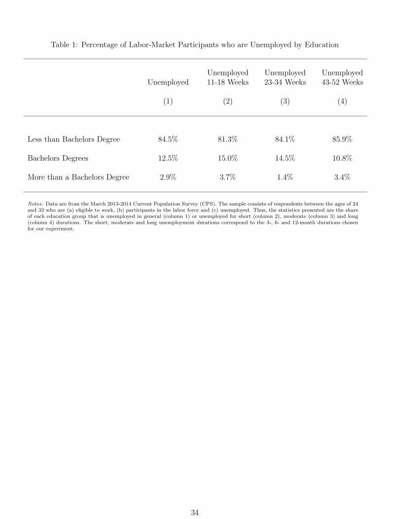
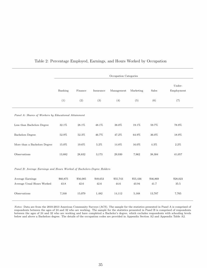
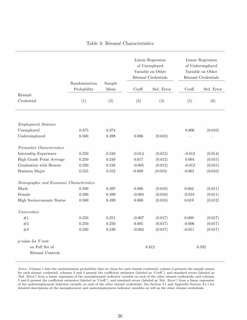


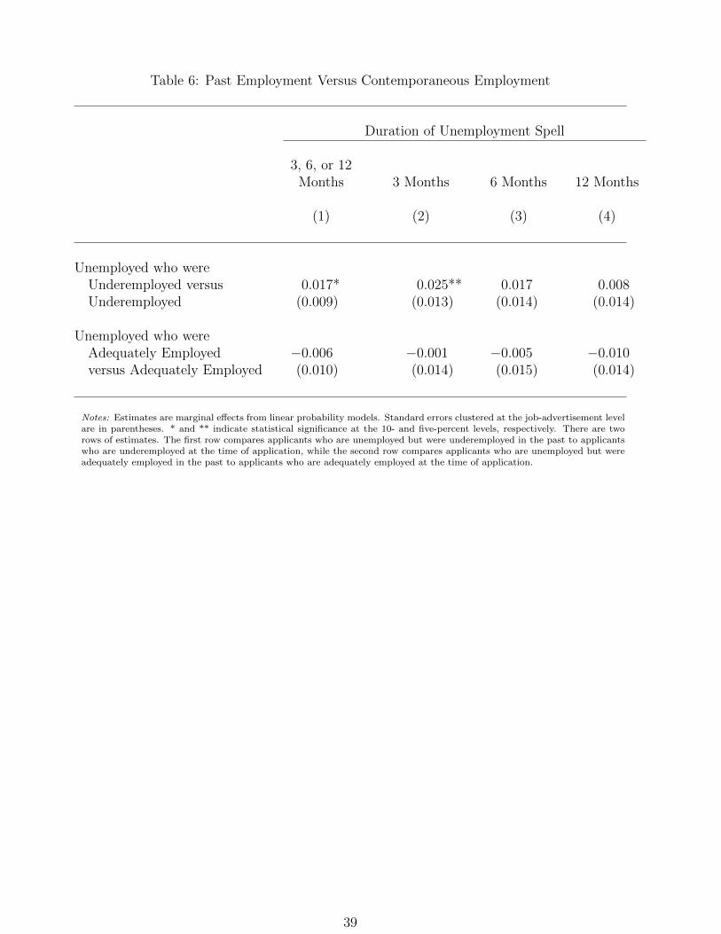
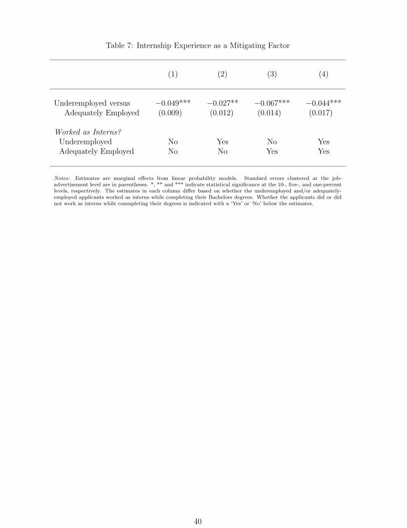
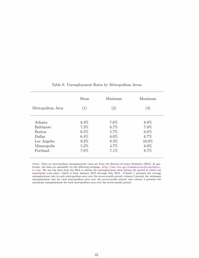
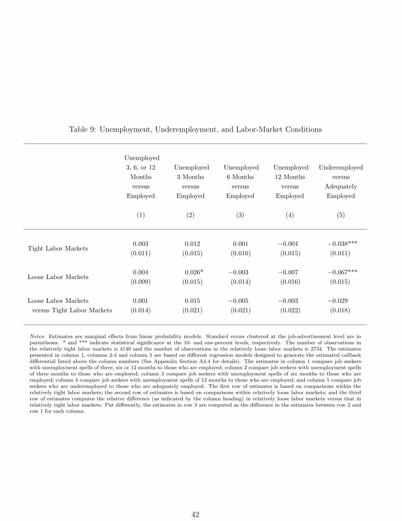


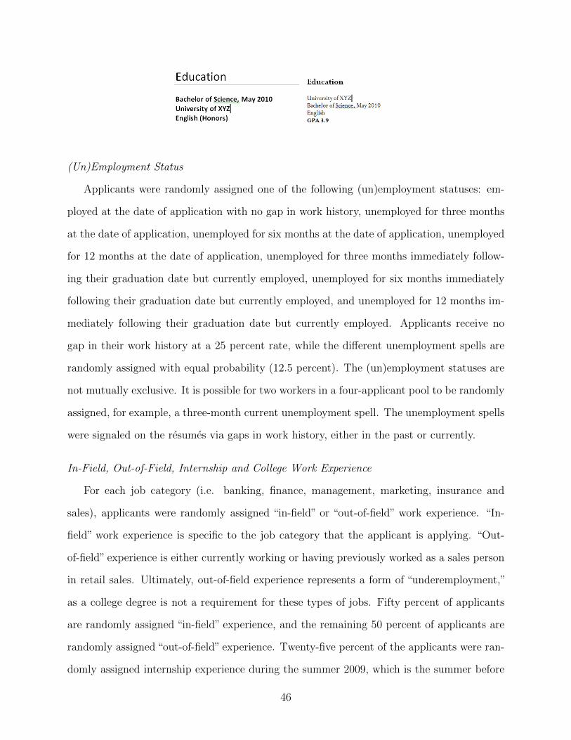

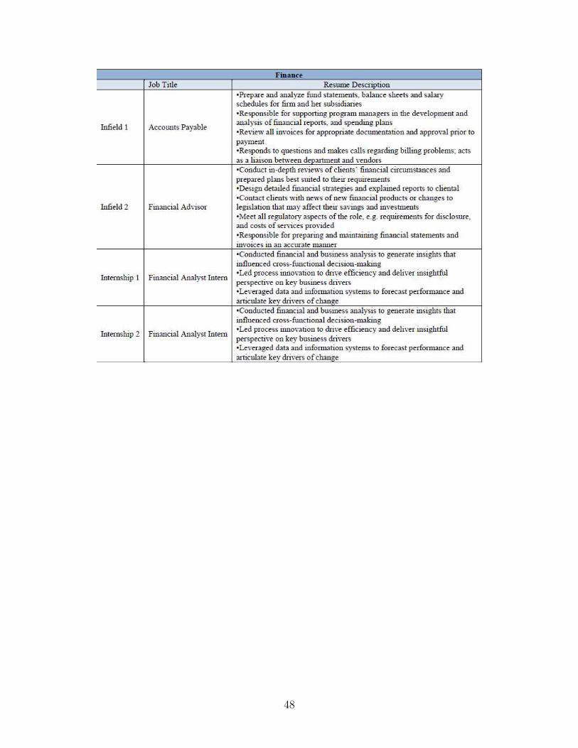
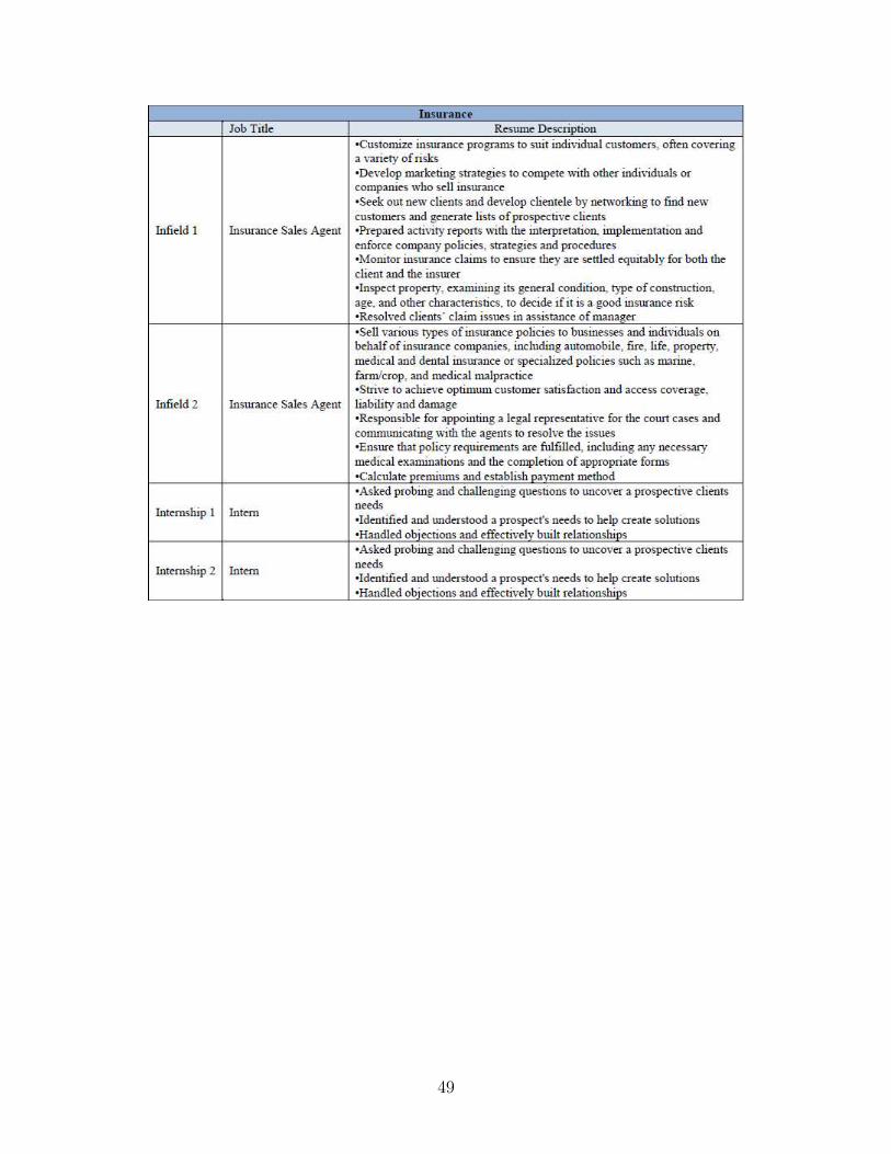
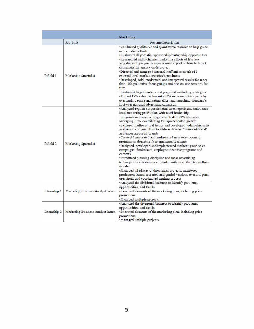
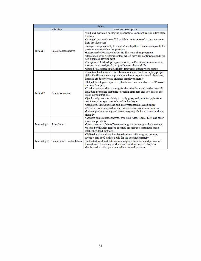


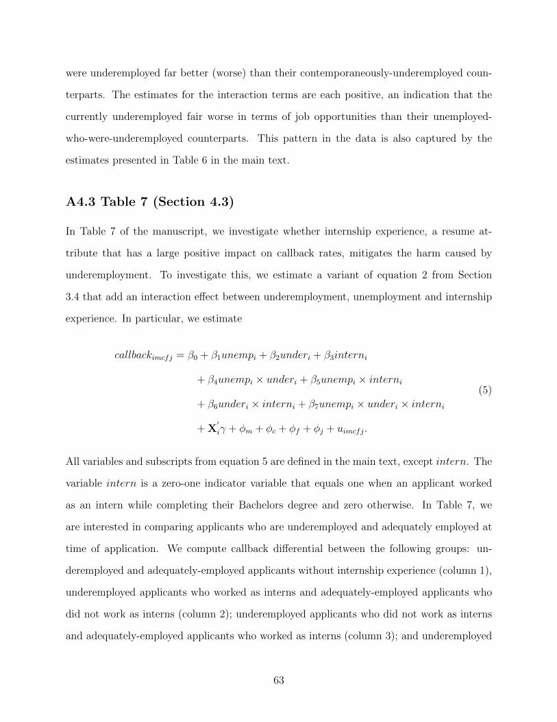


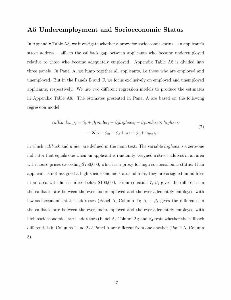
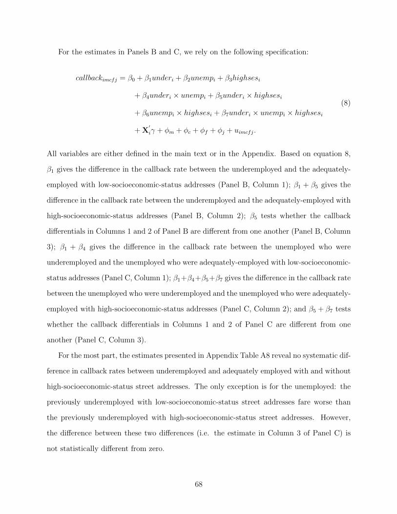
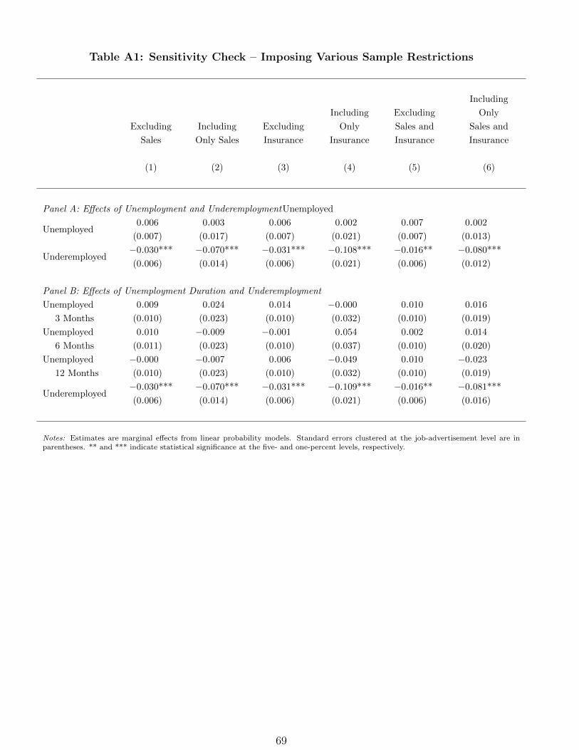
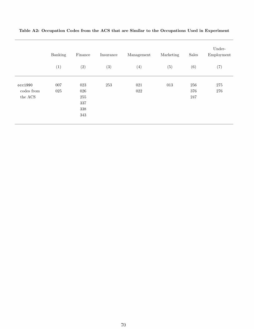
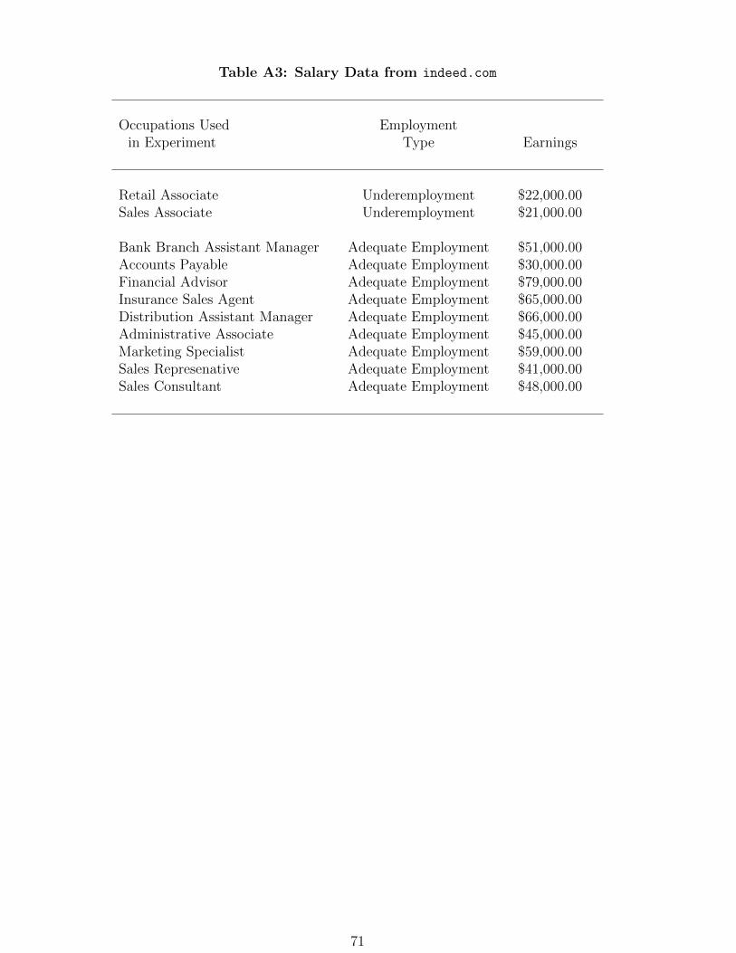


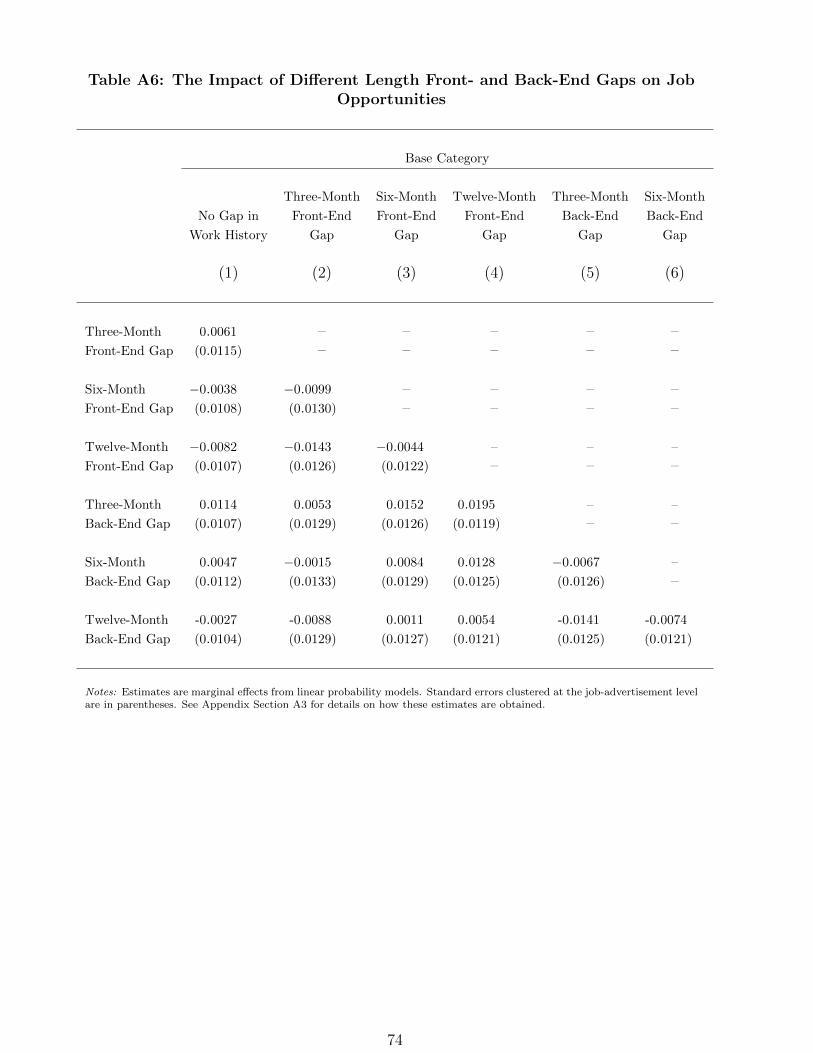
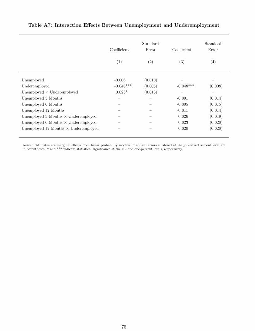
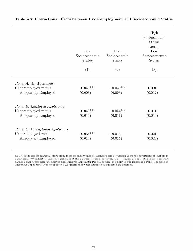
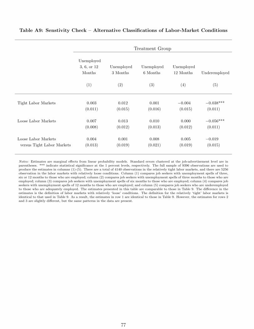


![[Baum Whiteman] 2013trends](https://static.documents.pub/doc/80x56/5451d6cbb1af9f7a248b4aba/baum-whiteman-2013trends.jpg)