Auckland Evacuation Model: development and calibration

Auckland evacuation model: development and calibration M. Afzal, S.B.Costello, P.Ranjitkar Page 1

Transportation Group 2019 Conference, Te Papa, 3-6 March 2019

Auckland Evacuation Model: development and calibration

*Mujaddad Afzal, PhD Student, Civil and Environmental Engineering, The University of Auckland, [email protected]

Dr Prakash Ranjitkar, PhD, Senior Lecturer, Civil and Environmental Engineering, The University of Auckland, [email protected]

Associate Professor Seosamh B. Costello, Deputy Head of Department, Civil and Environmental Engineering, The University of Auckland, [email protected]

*Corresponding author/presenter

mailto:[email protected]





Auckland Evacuation Model: Development and Calibration

Mujaddad Afzal, Prakash Ranjitkar, Seosamh B. Costello

ABSTRACT

This paper reports on the development and calibration of a base traffic simulation model for emergency planners to test different contingency plans for the emergency evacuation of Auckland city. The city was divided into 411 inhabited unit areas, with the most congested unit areas situated on an active volcanic field. The road network of these unit areas was imported into simulation software from open street maps, and fine-tuned by comparing with google maps and Auckland Council GEOMAPS. It was checked thoroughly and corrections were made for network errors such as movements at intersections, number of lanes, speed limit, capacity, etc. A normal day interim O-D matrices, fixed control plans and detector loop count data were obtained from the Auckland Forecasting Centre and loaded into the road network as base input parameters to train the base model and modelled counts and real counts during a normal day were compared to calibrate the model. The O-D matrices were then adjusted at screen lines using the “Frank and Wolf” static assignment method. While adjusting the O-D matrices, loop counts were considered 100 percent reliable and O-D trips were allowed to fluctuate. This fluctuation is allowed at screen lines, which cover major links, on-ramps, and off-ramps. The model was calibrated macroscopically by O-D matrix adjustment. Then volume based actuated control plans were generated using macroscopic simulation traffic volumes. These actuated control plans were used in the mesoscopic model and the model was calibrated at the mesoscopic level using the gradient-based Dynamic User Equilibrium (DUE) method, which is recommended for complex networks. The paper outlines the process of development and calibration of the base model for Auckland evacuation scenarios. Further publications will describe the set-up and outputs from the model for evacuation planning under different evacuation scenarios.

1 Introduction

Auckland is the economic and social hub of New Zealand. The region generates 37 percent of the country’s GDP and houses 33.4 percent of the country’s population. It is also the home to 66 percent of the country’s top 200 companies. The Auckland port handles 32 percent of the country’s exports by value, and 61 percent of its imports. Auckland is an international gateway with more than two million people visiting the city annually (Statistics New Zealand, 2013; New Zealand Trade and Enterprise, 2016).

Auckland city is built on top of the Auckland Volcanic Field (AVF), which covers a 360km2 area and is the youngest basaltic field in the world on which an urban area is established (Kermode, 1992; Searle, 1964). Figure 1 shows the extent of the AVF (Lindsay et al., 2010). Geographically, Auckland is an isthmus resulting in a limited north-south transportation corridor, which can be a challenging factor given the threat of a volcanic eruption if the city needs to be evacuated. Determining Volcanic Risk in Auckland (DEVORA) has proposed 8 different eruption scenarios, which are scattered in the Auckland Volcanic Field (AVF). Each scenario has a different evacuation area. It is important to estimate the total evacuation time for each scenario to better design the contingency plan for Auckland city. However, to simulate these scenarios a base model is required, which covers a complete geographic area of AVF and adjoining areas which may be affected by AVF. This paper focuses on the development and calibration of that base model, which will represent the normal day traffic condition, and a normal day traffic count data will be used to train the base simulation model.

The rest of the paper is organized as follows. A brief history of AVF, eruption scenarios and the study area is discussed in Section 2. Software used to model evacuation and base simulation models are discussed in Section 3. Section 4 provides an overview of the methodology to calibrate the model macroscopically and O-D matrix adjustment. Section 5 explains the results of macroscopic and mesoscopic calibration, and in Section 6 concluding remarks are provided, along with future research



directions.

2 AUCKLAND VOLCANIC FIELD (AVF)

The AVF has over 50 eruptive vents and has erupted over 55 times in the past 250,000 years (Loughlin, Sparks, Brown, Jenkins, & Vye-Brown, 2015). Rangitoto is the most recent eruption, which was witnessed by early indigenous Maori 550 years ago (Lindsay, 2010). The AVF volcanos are generally monogenetic in nature, they erupt only once, and the next eruption center will be at a different location within the volcanic field. There is no spatial or temporal pattern available for an eruption. Indeed, the oldest (Pupuke) and the youngest (Rangitoto) vents are located next to each other. The location and timing of the next eruption are, therefore, unknown. The size of the next eruption is also difficult to predict, as the last eruption, Rangitoto, accounts for nearly half of the erupted volume of the field. It is also unclear whether this eruption is an anomaly or signals a change in the eruptive behaviour of the field (Loughlin et al., 2015).

GNS Science is continuously monitoring the AVF though the Auckland Volcanic Seismic Monitoring Network (Lindsay, 2010). If any activity is detected by this network, warning communications will be in accordance with the National Civil Defence Emergency Management Plan Order (2005), which outlines the responsibilities of GNS Science, Ministry of Civil Defence and Emergency Management (MCDEM), Auckland Civil Defence and Emergency Management Group (ACDEMG) and MetService regarding the emergency situation (Auckland Council, 2013). There have been no significant AVF or other volcanic activity evacuations in New Zealand in recent times and, as such, local data was not available for research and study purposes (Cole et al., 2005). Therefore, the New Zealand government ran Exercise Ruaumoko in 2008, to test New Zealand’s nationwide arrangements for responding to a major disaster resulting from a volcanic eruption in Auckland. The Mt Ruaumoko scenario was selected because it would affect the infrastructure severely (Deligne et al., 2015).

The Mt Ruaumoko Scenario spans a 10 week period (6th February – 14th April 2008) (Deligne et al., 2015). Research on Mt Maugataketake volcano (Brand et al., 2014) was used to explain surge severity and range. It was assumed that there would be complete destruction within a 2.5km radius of the eruption, severe damage to most structures and complete damage to weak structures from 2.5-4km and some damage to weaker structures from 4-6km (Brand et al., 2014).

In the Mt Ruaumoko Scenario, it was assumed that less than 24 hours will be required to evacuate a 5 km radius zone (Horrocks, 2008). However, this evacuation time has no scientific backing. Although a conclusive figure can be obtained by conducting an actual evacuation exercise, the next best solution is developing a simulation model. Tomsen, Lindsay, Gahegan, Wilson, & Blake (2014) simulated the Mt Ruaumoko scenario in TransCAD and suggested that more detailed simulation software should be used to simulate an Auckland evacuation, as the network has limited capacity and will face excessive demand during the evacuation. They stated that commuters had to travel

Figure 1: Auckland Volcanic Field (Lindsay et

al., 2010)



long distances and would also face congestion during Auckland evacuation, and that TransCAD has limitations under such conditions.

After conducting the Ruaumoko exercise, Determining Volcanic Risk in Auckland (DEVORA) brought together more than 40 researchers from various research organizations including GNS, RiskScape, Auckland Council, University of Auckland and Massey University to develop further scenarios. They proposed 7 more eruption scenarios to study in detail while recognizing that the next eruption could be anywhere in the AVF. Figure 2 shows all 8 new proposed scenarios developed by DEVORA and 5 old scenarios proposed by Auckland Regional Council (ARC) in 1999.

2.2 Extent of Study Area

The study area includes all of Auckland, as shown in Figure 3. However, the model will be more detailed where the eruption vents from the DEVORA scenarios are located, and less detailed further from the resulting evacuation areas.

3 MODELING EVACUATION

(Sheffi, Mahmassani, & Powell, 1982) were the first to model evacuation at the macroscopic level, using the NETVACL model. They used three basic input information: network description including links and nodes, spatial and temporal loading patterns (O-D matrix), and control parameters (speed, static traffic assignment, etc.). With the passage of time, a number of other macroscopic traffic simulation software were developed and used to analyse evacuation studies. Oak Ridge Evacuation Modeling System (OREMS), Dynamic Network Evacuation (DYNEV), Evacuation Traffic Information System (ETIS) (Moriarty, Ni, & Collura, 2007) and EMME/2 (Jones, Naude, Van Wyngaardt, & Marks, 2007) have been used to analyze evacuation plans. In New Zealand, Tomsen et al., (2014) used TransCAD to prepare an evacuation plan for Auckland city. They recommended using more sophisticated software to analyse the evacuation plan because Auckland is densely populated and the network is congested and TransCAD has limitations under these conditions. All these studies used the same input parameters to develop the base model.

Mesoscopic models use the same basic input parameters in evacuation planning; however, they cover congestion conditions and temporal effects better than macroscopic models, while still capable of covering a larger geographic region than microscopic models. Cube Avenue, TRANSIMS and TransModeler are examples of commercially used mesoscopic models used in evacuation modelling (Hardy, Dodge, Smith, Vásconez, & Wunderlich, 2008).

Microscopic models provide more detail than macroscopic and mesoscopic models, as they consider individual driver behavior, vehicle characteristics, and detailed road geometry. Such models are usually used to undertake operational analysis, but these can also be used for evacuation planning. AIMSUN, CORSIM, Paramics, Sim Traffic, and VISSIM are examples of commercially used microsimulation software for evacuation modelling (Hardy et al., 2008). VISSIM has been used for

Figure 2: Proposed DEVORA Scenarios

(Source: Leonard et al., 2016)



analysis of Evacuation of Galveston Island and Florida Keys, USA in the case of hurricanes (Chen et al., 2006; Chen, 2008). TRANSIM was used for evacuation analysis of the Gulf of Mexico (Zhang, Spansel, & Wolshon, 2013) and New Orleans (Naghawi & Wolshon, 2010) in the case of hurricanes. Among all these studies only Zhang et al. (2013) calibrated and validated the model based on previous Hurricanes Katrina (2005) and Gustav (2008) evacuation. After calibration, they tested different evacuation scenarios for future evacuation.

However, in the case of Auckland, there has not been a volcanic eruption for 550 years. Hence, no traffic data available during the evacuation. Therefore, a normal day traffic count data is used to train the base simulation model. This type of simulation model can be used to analyse transportation system for an operational and planning purpose such as infrastructure improvement, demand management, congestion pricing, Intelligent transportation system (ITS) evaluation (Mahmassani, 2001; Ziliaskopoulos, Waller, Li, & Byram, 2004). These models represent normal day traffic conditions and calibrated and validated using normal day traffic data (Flötteröd et al., 2011; Ben-Akiva et al., 2012; Duell et al., 2016).

Flötteröd et al. (2011) calibrated the Dynamic simulation model using loop detector count data. Ben-Akiva et al. (2012) calibrated the model of a sub-area of Beijing, China using loop detector count data and floating car travel time data. Duell et al. (2016) calibrated the model of Sydney, Australia at macroscopic and mesoscopic level, using speed points across the network.

In this study, loop detector count data is used to calibrate the base model in AIMSUN simulation environment, as it provides integration of macro, meso and micro models in one package. Moreover, the New Zealand Transport Agency and Auckland Transport use AIMSUN and it will, therefore, be easier to integrate with these agencies.

4 BASE MODEL

Base model preparation is the first step in evacuation traffic modelling. Base model calibration depends on the accessibility and quality of inputted data. Data, including but not limited to, the road network, Origin and Destination (O-D) data, speed limits, signal phasing and traffic counts of study areas were made available from the Auckland Forecasting Centre (AFC) and open sources. An iterative process was used to calibrate the base model in which the parameters were adjusted until the simulation results coincided with observed field results (Ni et al., 2004; Ben-Akiva et al., 2012). The process is as follows:

1. Open Street Map (OSM) was imported into AIMSUN and the road network attributes (lane number and configuration, and connections) were amended using the most up-to-date images on Google Maps and Auckland GEOMAPS.

2. Intersections (nodes) were fine-tuned, detectors were installed, and signal phasing configuration was employed.

3. Speed limits were checked, and the interim O-D matrix was uploaded. After that, the simulation was run.

4. The modelled counts were compared with actual counts using NZTA criteria. If the criteria were met, then the model was deemed calibrated. If not, then the network attributes (links, nodes, speed limits, signal phasing etc.) were fine-tuned.

4.1 Calibration Criteria

Economic Evaluation Manual (NZTA, 2008) provides transport modelling checks, which were used as the calibration criteria for the base model. These checks are further refined by Transport Model Development Guidelines (NZTA 2014). These checks are also recommended by the Economic Evaluation Manual (NZTA, 2016). The details of the checks which will be considered in this research are as follows:



Link Volume Plot (Mandatory Check)

Modelled and observed link volumes for each time period were compared and the differences between them were observed. The total volume at all screen lines was summarised and the error tolerance was checked. The error tolerances for individual links and screenlines are illustrated in Table 1. Where errors fall outside reasonable tolerances, the relevant links will be highlighted on the link volume plot.

XY Scatter Plot (Mandatory Check)

This check includes the comparison of observed and modelled flow for individual links and screenlines. The line x = y was superimposed on each plot and the R2 coefficient was checked. NZTA (2008) proposed that the R2 coefficient should be greater than 0.85, and greater than 0.95 near the area of interest. The NZTA Transport Model Development Guidelines (NZTA 2014) also recommend an R2 value of 0.85 for regional models. Table 2 shows the NZTA (2014) calibration criteria.

GEH Statistic (Recommended Check)

The GEH value criteria should be satisfied according to the EEM (2008). At least 60% of individual link flows should have a GEH less than 5.0. At least 95% of individual link flows should have a GEH less than 10.0. All individual link flows should have a GEH less than 12.0. Screen line flows should have a GEH less than 4.0 in most cases. GEH value is a form of Chi-squared statistic which is designed to be tolerant of larger errors in low flows. It is computed for individual and screenline hourly link flows. The GEH statistic has the following form as Equation 1:

𝐺𝐸𝐻 = √2(𝑞𝑚𝑜𝑑𝑒𝑙 − 𝑞𝑜𝑏𝑠)

(𝑞𝑚𝑜𝑑𝑒𝑙 − 𝑞𝑜𝑏𝑠) (1)

Where qobs = observed hourly flow

qmodel = modelled hourly flow

Further detail of GEH criteria for each type of network is explained in the NZTA Transport Model Development Guidelines (2014), which are shown in Table 3.

Percentage Root Mean Square Error (RMSE) (Recommended Check)

Unlike the GEH statistic (which applies to individual flows and screenlines), the root–mean–square error applies to the entire network. Generally, the RMSE should be less than 30%. The percentage RMSE is calculated as shown in Equation 2:

S.N. Link Type Volume Error Tolerance

01 Individual major link <15,000 veh/day ±20%

02 Individual major link >15,000 veh/day <±20%

03 Screen lines ±10%

Table 1: Link Volume Error Tolerance (NZTA, 2008)

Statistic

Model Category

A:

Regional

B:

Strategic Network

C:

Urban Area

D:

NZ Transport Agency Project

E:

Small Area / Short

Corridor

F:

Intersection / Short

Corridor

G:

High Flow,

Speed, Multi lane

R2 Value >0.85 >0.9 >0.95 >0.95 >0.95 >0.95 >0.95

Table 2: XY Scatter Plot criteria (NZTA, 2014)



%𝑅𝑀𝑆𝐸 = √

∑(𝑞𝑚𝑜𝑑𝑒𝑙 − 𝑞𝑜𝑏𝑠)2

(𝑁𝑢𝑚𝑏𝑒𝑟 𝑜𝑓 𝑐𝑜𝑢𝑛𝑡𝑠−1)

∑ 𝑞𝑜𝑏𝑠𝑁𝑢𝑚𝑏𝑒𝑟 𝑜𝑓 𝑐𝑜𝑢𝑛𝑡𝑠

× 100 (2)

Calibration of models are important to ensure that the simulation is as accurate as possible and a close replica of the real conditions. Model calibration is an iterative process in which simulation constants and parameters are adjusted until the simulation results coincide with observed field results. The model produces results that represent the true system behaviour and can be used as a substitute for experimental purposes (Ni et al., 2004).

4.2 Road Network

The accuracy of any simulation model depends on the accuracy of the inputted data. The development of the road network was the first step in preparing the base model. The road network was imported into AIMSUN using Open Street Maps (OSM). The OSM template does not produce 100 percent accurate road layout. Therefore, each road segment and intersection/interchange was checked individually to ensure that the network represents actual field conditions, using the most up-to-date images on Google Maps. The main motorways, highways, arterial and main collector roads were included in this model. Some local streets were not included, and trips generated from these zones were distributed around the nearest modelled local/collector link.

Auckland Transport classifies the links into two categories: arterial and non-arterial links. Arterial links are further sub-divided into the sub-categories: motorways, strategic routes, primary and

Table 3: Hourly GEH Comparison Criteria (Source: NZTA, 2014)



secondary arterial roads. Non-arterial links are further sub-divided into sub-categories: collector roads, local streets, lanes and service lanes, shared space / shared zones (Auckland Transport, 2017). Figure 3 shows the road network developed in the AIMSUN model. All motorways (100 km/hr) and ramps (70 km/hr) are coded in the colour green, other arterials (50 km/hr) are coded in blue and strategic roads are coded in orange (60 km/hr), purple (70 km/hr) and yellow (80 km/hr), collectors (50 km/hr) are coded in red, rural roads are coded in black (50-100 km/hr).

After defining the road network, attributes and control parameters for each segment of the network were defined in detail. This includes the number of lanes of each link, turning bays, speed limits and give-way signs, where applicable. All Intersections were checked and turning movements at each intersection were defined, also major and minor links were defined.

After defining the physical and operational characteristics of the network, an interim Origin and Destination (O/D) matrix and real-time count data were uploaded in the model, both of which were made available from the Auckland Forecasting Centre.

4.3 Assumptions

The following assumptions were made to construct the base model:

• Driver behaviour would not be reckless, and standard road rules would be followed by all road users. The authors are aware that this may be unrealistic, and will update this as part of further research as such data becomes available.

• All signalized intersections were assumed to operate under fixed control in the macroscopic model, and volume based actuated control in the mesoscopic model.

• PM Peak hour time of day was selected to calibrate the model because it represents the worst-case scenario for regional roadway network traffic congestion, and traffic conditions during that time are closer to evacuation conditions (de Araujo et al., 2011).

• Outside of the potential eruption unit areas, only the arterial roads, state highways and collector roads were retained. This simplification assumed that drivers would travel on any road in the network initially (Moriarty et al., 2007), but once outside their locality, they would travel on the main/familiar routes (Lindell and Prater, 2007).

Figure 3: Roads in Auckland Road Network (AIMSUN

Model)



5 MODEL CALIBRATION

5.1 Macroscopic Model Calibration

The macroscopic model base year was taken as March 2016. It had 691 fixed control intersections and 817 count detectors. The simulation time was PM peak (3:00 to 7:00 PM) and 30 iterations were run to get results using the “Frank and Wolf” traffic assignment method.

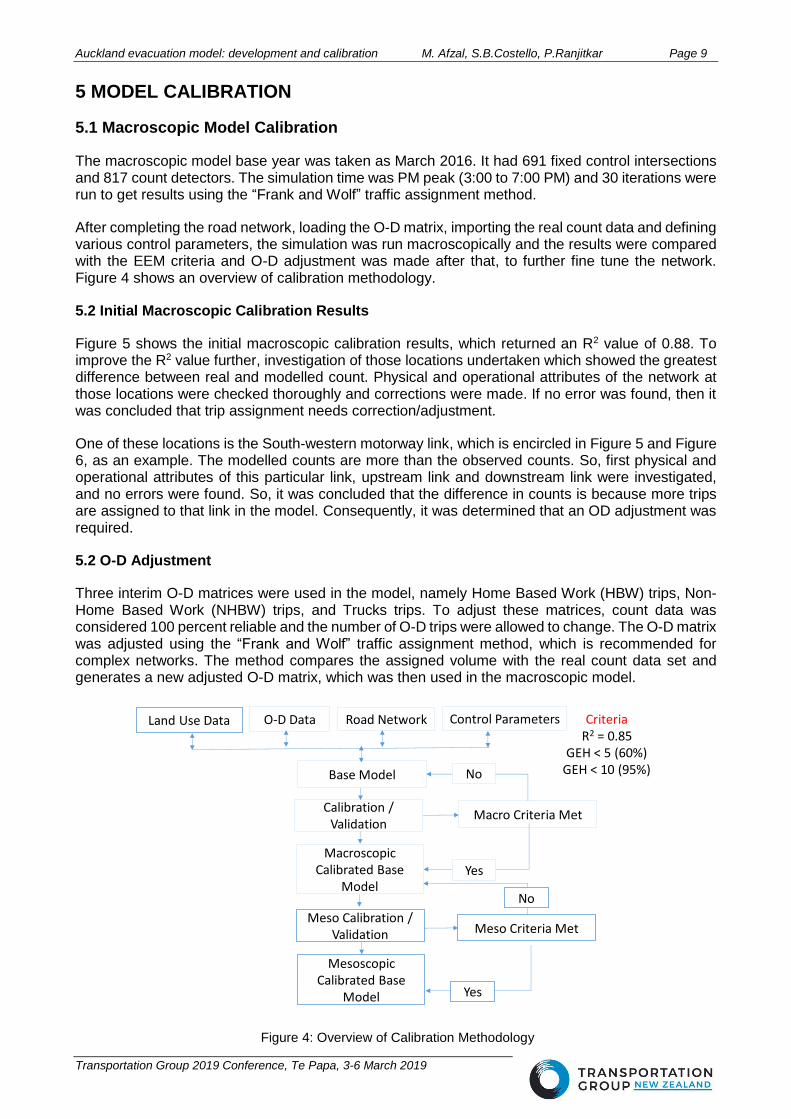
After completing the road network, loading the O-D matrix, importing the real count data and defining various control parameters, the simulation was run macroscopically and the results were compared with the EEM criteria and O-D adjustment was made after that, to further fine tune the network. Figure 4 shows an overview of calibration methodology.

5.2 Initial Macroscopic Calibration Results

Figure 5 shows the initial macroscopic calibration results, which returned an R2 value of 0.88. To improve the R2 value further, investigation of those locations undertaken which showed the greatest difference between real and modelled count. Physical and operational attributes of the network at those locations were checked thoroughly and corrections were made. If no error was found, then it was concluded that trip assignment needs correction/adjustment.

One of these locations is the South-western motorway link, which is encircled in Figure 5 and Figure 6, as an example. The modelled counts are more than the observed counts. So, first physical and operational attributes of this particular link, upstream link and downstream link were investigated, and no errors were found. So, it was concluded that the difference in counts is because more trips are assigned to that link in the model. Consequently, it was determined that an OD adjustment was required.

5.2 O-D Adjustment

Three interim O-D matrices were used in the model, namely Home Based Work (HBW) trips, Non-Home Based Work (NHBW) trips, and Trucks trips. To adjust these matrices, count data was considered 100 percent reliable and the number of O-D trips were allowed to change. The O-D matrix was adjusted using the “Frank and Wolf” traffic assignment method, which is recommended for complex networks. The method compares the assigned volume with the real count data set and generates a new adjusted O-D matrix, which was then used in the macroscopic model.

Figure 4: Overview of Calibration Methodology

Road Network

Macroscopic Calibrated Base

Model

Base Model

Control ParametersO-D Data

Calibration / Validation

Macro Criteria Met

Yes

No

CriteriaR2 = 0.85

GEH < 5 (60%)GEH < 10 (95%)

Meso Criteria Met

Yes

No

Mesoscopic Calibrated Base

Model

Meso Calibration / Validation

Land Use Data



5.3 Final Macroscopic Calibration Results

After O-D adjustment, path assignments, which were generated during O-D adjustment, were loaded in the model. Then, 30 iterations were run using the “Frank and Wolf” assignment model. An R2 value of 0.98 was achieved. Hence, the model was considered calibrated macroscopically. Figure 7 shows the final calibration results and Table 4 shows the change in demand after O-D adjustment. Figure 8 shows the counts at the South-Western Motorway link after O-D adjustment. Red shows the assigned count at the link before O-D adjustment and blue shows assigned count after O-D adjustment, which is similar to the real count shown in light blue.

5.4 Mesoscopic Calibration

Subsequently, the model was calibrated at the mesoscopic level. The gradient-based Dynamic User Equilibrium (DUE) method was used to run the scenario with 30 minutes of warmup time. The gradient-based method is recommended for complex networks. The O-D matrix and path assignments from the macroscopic model were loaded into the mesoscopic model, and each parameter of the mesoscopic model was then fine-tuned, step by step. A list of sensitivity parameters is listed in Table 5.

First, the sensitivity of the Reaction Time (RT) factor was checked, as this is the most sensitive parameter. RT values were varied, and the rest of the parameters were fixed. For example, for the first iteration, the Reaction Time factor at the traffic light was given a value of 1.6 sec, jam density for motorway and urban roads was assumed to be 180 vehicle/km, the initial and final safety margin for the motorways were given values of 7.5 sec and 4.5 sec, respectively, and initial and final safety margins for urban roads were given values of 6 sec and 3 sec, respectively. The results are as follows in Table 6. These results are obtained using

Figure 5: Initial Macroscopic Calibration Results (0.88 R2 Value)

Figure 6: South Western Motorway

Figure 7: Final Macroscopic Calibration results (0.98 R2 Value)



interim O-D matrices, and macroscopically adjusted O-D matrices are not used at this stage.

The macroscopically adjusted O-D Matrices and path assignments were used later in the network to improve the R2 value. Table 7 shows the 5 iteration results, with the same parameters.

At this stage, an R2 value of 0.68 was achieved and it was difficult to further improve the R2 value. The minimum requirement is 0.85. However, it was noted that the network was heavily congested. To observe the congestion in the model, some sections of the model were converted into microsimulation sections and a hybrid simulation was run. In this simulation, only the particular section of the model under investigation at the time was run microscopically, and the rest of the model behaved as a dynamic scenario.

The hybrid simulation showed that most of the intersections became heavily congested after 1 hour and 45 minutes of simulation. Figure 9 shows the flow conditions at the Southern Motorway. Most links exhibited the same, congested, traffic conditions and vehicles were unable to move in the network. It was assumed that this condition was due to an improper signal control plan, as at that stage, fixed signal control plans were used in the model. Consequently, volume-based actuated traffic control plans were generated using macroscopic traffic volumes. These actuated traffic control plans were used and simulations were run again, returning an R2 value of 0.90. However, the results in Figure 10 show many points below the diagonal red line - the line of equality, where X and Y are exactly the same. These points are the locations on the network where the modelled traffic counts are underestimated, as compared to observed traffic counts.

Figure 8: Comparison between Modelled and Observed Count after OD

Adjustment

Total Demand PM Peak (3pm- 7pm)

Pre- Adjustment (Vehicle) 1,143,390

Post-Adjustment (Vehicle) 1,124,800

Change (Vehicle) 18,590

Change (%) 1.62 %

Table 4: Change in Demand after OD Adjustment



Achieving a 0.90 R2 value shows that the model provides satisfactory results as a whole system. However, some links in the model are still not simulating real-time results at the mesoscopic level. Flow at these links can be improved further by improving the GEH value at those links. Figure 11 shows the GEH values at different links in the network. The green dots represent a 0-5 GEH value, the orange dots represent a 5-10 GEH value and the red dots represent a greater than 10 GEH value. The red dots are those locations in the network which need fine tuning. Overall 49.69% of count locations have less than a 5 GEH value and 77.72% of count locations have less than a 10 GEH value. These should be at least 60 % and 95 % according to NZTA criteria.

Sr. No.

Parameters (AIMSUN Standard Value)

Range Sensitivity Comments

1 Reaction Time (RT) Factor

(1.20) 1.15 1.2 1.25 very sensitive

1.15 to 1.25 recommended range

2 Reaction Time Factor at

Traffic Light (1.60) 1.6 2.1 2.8 less sensitive

2.8 for 50km/h recommended

3 Jam Density: section

parameter (180) 200 180 160

moderate sensitive

depends upon local condition

4 Final Safety Margin: turn

parameter 3 4.5 6

moderate sensitive

must be lower to improve turning flow

5 Initial Safety Margin: turn

parameter 6 7.5 9 don’t know

6 Traffic Assignment Model

Type Gradient Based

Weighted MSA

MSA very sensitive

Table 5: List of AIMSUN Parameters

Sr. No.

Reaction Time (RT) Factor

Gradient Based (R2 Value)

Weighted MSA (R2 Value)

MSA (R2 Value)

Comments

1 1.10 0.426

2 1.15 0.444 0.423 0.419 Gradient Based assignment with

1.15 RT gives best results R2 Value

3 1.20 0.34

4 5 iteration (1.15) 0.463

Table 6: Mesoscopic Calibration Initial Results (3 iterations)

Sr. No.

Parameters R2 Value Comments

1 Path Cost Assignment loading

pattern 5 Iterations

2 Instantaneous Start assignment

process 0.6719

3 Experience Start assignment

process 0.6766

Experience path cost gives the better R2 value.

4 Experience Continuous assignment

process 0.6766

Table 7: Mesoscopic Calibration Second Results (5 iterations)



Figure 9: Flow condition: Congested Network

Figure 10: Mesoscopic Third Results (0.90 R2 Value)

Figure 11: Mesoscopic GEH Value Third Results



6 CONCLUSION AND FURTHER RESEARCH

This paper documents the first part of a project that aims to assess the resilience of the Auckland city network against volcanic eruption. It describes the development and calibration of a base model for the Auckland road network, which will be used to run different evacuation scenarios. The base model was initially calibrated macroscopically. Afterwards, O-D Matrices were adjusted and new O-D matrices were generated. These matrices were used to further fine-tune the macroscopic model. Subsequently, the base model was calibrated mesoscopically.

The macroscopic base model basic input parameters were a road network, O-D Matrices, Fixed Control Plans and a real data set of traffic counts at 817 locations. The road network was calibrated by comparing modelled counts and observed data and 0.98 R2 value was achieved, which meets NZTA criteria. Subsequently, the mesoscopic model was calibrated. The input parameters used in the mesoscopic model were the calibrated road network and adjusted O-D matrices from the macroscopic model, volume-based actuated traffic control plans (which were generated using macroscopic simulated traffic volume in the network) and a real data set of traffic counts. An R2 value of 0.90 was achieved, which also meets NZTA criteria. However, the model could not exactly meet the NZTA criteria for the GEH value. This shows that the network is performing well as a complete system, but some individual links are under- or over-estimating the traffic flows.

Further investigation of individual links will be conducted to improve the GEH value and the model will be validated either using travel time data or another set of count data. The model can be used to assess preliminary evacuation scenarios at this stage and preliminary results can be extracted, as the model is providing a 0.90 R2 value as a complete system.

REFERENCES

Brand, B. D., Gravley, D. M., Clarke, A. B., Lindsay, J. M., Bloomberg, S. H., Agustin-Flores, J., & Németh, K. (2014). A combined field and numerical approach to understanding dilute pyroclastic density current dynamics and hazard potential: Auckland Volcanic Field, New Zealand. Journal of Volcanology and Geothermal Research, 276, 215-232.

Chen, X. (2008). Microsimulation of hurricane evacuation strategies of Galveston Island. The Professional Geographer, 60(2), 160-173.

Chen, X., Meaker, J. W., & Zhan, F. B. (2006). Agent-based modeling and analysis of hurricane evacuation procedures for the Florida Keys. Natural Hazards, 38(3), 321-338.

Cole, J., Sabel, C., Blumenthal, E., Finnis, K., Dantas, A., Barnard, S., & Johnston, D. (2005). GIS-based emergency and evacuation planning for volcanic hazards in New Zealand.

de Araujo, M. P., Casper, C., Lupa, M. R., Brinckerhoff, P., Waters, B., & Hershkowitz, P. (2011). Adapting a four-step MPO travel model for wildfire evacuation planning: A practical application from colorado springs.

Deligne, N. I., Blake, D. M., Davies, A. J., Grace, E. S., Hayes, J., Potter, S. H., . . . Wilson, T. M. (2015). Economics of Resilient Infrastructure Auckland Volcanic Field scenario GNS Science.

Duell, M., Saxena, N., Chand, S., Amini, N., Grzybowska, H., & Waller, S. T. (2016). Deployment and Calibration Considerations for Large-Scale Regional Dynamic Traffic Assignment: Case Study for Sydney, Australia. Transportation Research Record: Journal of the Transportation Research Board, (2567), 78-86.

Economic Evaluation Manual (2008). New Zealand Transport Agency (NZTA). Retrieved from NZTA. https://www.nzta.govt.nz/assets/resources/economic-evaluation-manual/volume-1/docs/eem1-amendment-2-pages.pdf

https://www.nzta.govt.nz/assets/resources/economic-evaluation-manual/volume-1/docs/eem1-amendment-2-pages.pdf

https://www.nzta.govt.nz/assets/resources/economic-evaluation-manual/volume-1/docs/eem1-amendment-2-pages.pdf



Economic Evaluation Manual (2016). New Zealand Transport Agency (NZTA). Retrieved from NZTA. https://www.nzta.govt.nz/assets/resources/economic-evaluation-manual/economic-evaluation-manual/docs/eem-manual-2016.pdf

Hardy, M., Dodge, L., Smith, T., Vásconez, K. C., & Wunderlich, K. E. (2008). Evacuation management operations modeling assessment: Transportation modeling inventory. 15th World Congress on Intelligent Transport Systems and ITS America's 2008 Annual Meeting ITS America ERTICOITS Japan TransCore.

Jones, J., Naude, S., Van Wyngaardt, G., & Marks, A. (2007). Koeberg nuclear emergency plan: Traffic evacuation model. Satc 2007,

Kermode, L. (1992). Geology of the Auckland urban area, Scale 1: 50000, Institute of Geological and Nuclear Sciences Geological map2. Institute of Geological and Nuclear Sciences Ltd., Lower Hutt, New Zealand, 1

Leonard, G., Lindsay, J. M., Smith, R., Woods, R. (2016). DeVoRA – Summary of research to date and opportunities for the future. [PowerPoint Slides].

Lindsay, J. M., Marzochi G. J., Constantinescu, R., Selva, J. & Sandri, L. (2010). Toward real-time eruption forecasting in the Auckland Volcanic Field: application of BET_EF during the New Zealand National Disaster Exercise Ruaumoko. Bulletin of Volcanology, 72(2), pp.185-204.

Lindsay, J. M. (2010). Volcanoes in the big smoke: a review of hazard and risk in the Auckland Volcanic Field. In Geologically Active, Delegate Papers of the 11th Congress of the International Association for Engineering Geology and the Environment (IAEG).

Lindell, M. K. & Prater, C. S. (2007). Critical behavioral assumptions in evacuation time estimate analysis for private vehicles: Examples from hurricane research and planning. Journal of Urban Planning and Development, 133(1), 18-29.

Loughlin, S. C., Sparks, R. S. J., Brown, S. K., Jenkins, S. F., & Vye-Brown, C. (2015). Global volcanic hazards and risk Cambridge University Press.

Mahmassani, H. S. (2001). Dynamic network traffic assignment and simulation methodology for advanced system management applications. Networks and Spatial Economics, 1(3-4), 267-292.

Moriarty, K. D., Ni, D., & Collura, J. (2007). Modeling traffic flow under emergency evacuation situations: Current practice and future directions.

Naghawi, H., & Wolshon, B. (2010). Transit-based emergency evacuation simulation modeling. Journal of Transportation Safety & Security, 2(2), 184-201.

Ni, D., Leonard, J., Guin, A., & Williams, B. (2004). Systematic approach for validating traffic simulation models. Transportation Research Record: Journal of the Transportation Research Board, (1876), 20-31.

Searle, E. J. (1964). City of Volcanoes: a geology of Auckland Paul's Book Arcade.

Sheffi, Y., Mahmassani, H., & Powell, W. B. (1982). A transportation network evacuation model. Transportation Research Part A: General, 16(3), 209-218. doi:http://dx.doi.org.ezproxy.auckland.ac.nz/10.1016/0191-2607(82)90022-X

Tomsen, E., Lindsay, J. M., Gahegan, M., Wilson, T. M., & Blake, D. M. (2014). Evacuation planning in the Auckland Volcanic Field, New Zealand: a spatio-temporal approach for emergency management and transportation network decisions. Journal of Applied Volcanology, 3(1), 6.

Transport model development guidelines (2014). New Zealand Transport Agency (NZTA). Retrieved

https://www.nzta.govt.nz/assets/resources/economic-evaluation-manual/economic-evaluation-manual/docs/eem-manual-2016.pdf

https://www.nzta.govt.nz/assets/resources/economic-evaluation-manual/economic-evaluation-manual/docs/eem-manual-2016.pdf

http://dx.doi.org.ezproxy.auckland.ac.nz/10.1016/0191-2607(82)90022-X



from NZTA. https://www.nzta.govt.nz/assets/resources/transport-model-development-guidelines/docs/tmd.pdf

Zhang, Z., Spansel, K., & Wolshon, B. (2013). Megaregion network simulation for evacuation analysis. Transportation Research Record: Journal of the Transportation Research Board, (2397), 161-170.

Ziliaskopoulos, A. K., Waller, S. T., Li, Y., & Byram, M. (2004). Large-scale dynamic traffic assignment: Implementation issues and computational analysis. Journal of Transportation Engineering, 130(5), 585-593.

Acknowledgment The authors would like to thank the National Science Challenge (NSC) – Resilience to Nature’s Challenges (RNC) and the University of Auckland for funding this research. Additional thanks to the Auckland Forecasting Centre (AFC) for providing data and support.

https://www.nzta.govt.nz/assets/resources/transport-model-development-guidelines/docs/tmd.pdf

https://www.nzta.govt.nz/assets/resources/transport-model-development-guidelines/docs/tmd.pdf

Date post:	07-Apr-2022
Category:	Documents
Upload:	others
View:	3 times
Download:	0 times

Auckland Evacuation Model: development and calibration

Documents