Page 1
Munich Personal RePEc Archive
Auction Market System in Electronic
Security Trading Platform
Li, Xi Hao
Department of Economics and Social Sciences (DiSES)
2012
Online at https://mpra.ub.uni-muenchen.de/43183/
MPRA Paper No. 43183, posted 09 Dec 2012 20:08 UTC
Page 2
Auction Market System in Electronic Security
Trading Platform
Li Xihao∗
Working Paper
December 8, 2012
Abstract
Under the background of the electronic security trading platform Xetra oper-
ated by Frankfurt Stock Exchange, we consider the Xetra auction market system
(XAMS) from ‘bottom-up’, which the interaction among heterogeneous traders
and Xetra auction market mechanism generates non-equilibrium price dynamics.
First we develop an integrative framework that serves as general guidance for
analyzing the economic system from ‘bottom-up’ and for seamlessly transferring
the economic system into the corresponding agent-based model. Then we apply
this integrative framework to construct the agent-based model of XAMS. By
conducting market experiments with the computer implementation of the agent-
based model of XAMS, we investigate the role of the price setter who assumes
its trading behavior can manipulate the market price. The main finding is that
the introduction of the price setter in the setting of XAMS improves market
efficiency while does not significantly influence price volatility of the market.
Keywords: agent-based modeling, computational market experiment, electronic
security trading platform, Xetra, non-equilibrium price dynamics,
automatic trading.
JEL Classification: B4, C6, C9, D4, D5, D6, G1.
∗Department of Economics and Social Sciences (DiSES), Polytechnic University of Marche,
Ancona, Italy. Email: [email protected] .
1
Page 3
1 Introduction
Electronic security trading platforms operated by stock exchanges are prevail-
ing in global financial markets, e.g. Xetra (Frankfurt Stock Exchange), SETS
(London Stock Exchange), and Universal Trading Platform (NYSE Euronext).
This new generation of trading platforms enables market participants (brokers,
dealers, institutional and retail investors) to trade on electronic order books via
remote computer access. Electronic trading platforms explicitly stipulate mar-
ket mechanisms for determining the trading price and the trading volume even
when the market is not in equilibrium, e.g. see (Gruppe Deutsche Borse, 2003)
and (NYSE Euronext, 2010). On the other hand, market participants, especially
institutional investors, are competing against each other to utilize the knowledge
on market mechanisms and the real-time market data to generate trading strate-
gies in order to exploit the market for a profit. The interaction among market
participants and market mechanisms in electronic trading platforms generates
market dynamics with non-equilibrium trading prices.
It is a challenging task to establish a financial market model for the electronic
trading platform as financial market models in economic literature generally fol-
low the assumption of the market equilibrium, e.g. see (Sharpe, 1964) and (Mer-
ton, 1992). The construction of the financial market model for the electronic trad-
ing platform requires three aspects. First, it requires a formalization of the market
mechanism in the electronic trading platform which allows non-equilibrium trad-
ing prices. Market mechanisms vary in electronic trading platforms, although
they implement the same fundamental principle of maximum trading volume to
determine the trading price. In this work we focus on one specific electronic
trading platform – Xetra system operated by Frankfurt Stock Exchange.
According to (Gruppe Deutsche Borse, 2003), Xetra system is an order driven
system which traders participate in by submitting their order specifications such
as limit orders or market orders. A limit order in Xetra is an order specification
to buy or sell indicated shares of the security at a specific price called limit
price or better. A market order is an unlimited order specification to buy or
sell the indicated shares at the next trading price. There are two trading forms
in Xetra: continuous trading and Xetra auction, which associate with different
market mechanisms. Our target is on Xetra auction which belongs to the type
of multi-unit double auction. It mainly consists of the call phase and the price
determination phase. During the call phase, traders submit order specifications
and Xetra auction market mechanism (XAMM) collects these orders into a central
order book without giving rise to transactions. The price determination phase
2
Page 4
follows when the call phase stops randomly after a fixed time span. Given the
central order book, XAMM determines the trading price and the trading volume
in the price determination phase by applying Xetra auction trading rules specified
in (Gruppe Deutsche Borse, 2003). We follow this line to consider an explicit
formulation of XAMM to determine the trading price and the trading volume in
the Xetra auction market model.
The second aspect is on the role that the knowledge on XAMM and the real-time
market data play in trader’s investment decision process. XAMM determines the
trading price according to the central order book which is an aggregation of orders
submitted by traders. This implies that the trader could potentially influence the
current trading price by submitting its order. With the knowledge on XAMM and
the real-time market data of the central order book, the trader can discover the
relationship between the current trading price and the trading quantity quoted
in its order in a step functional form, see (Li, 2010). By integrating this function
into the trader’s investment decision to determine its quoted trading quantity,
the trader realizes in its investment decision the potential of manipulating the
trading price by submitting its order. The trader is then called the price setter as
it can manipulate the trading price through its trading behavior in the market.
For example, institutional traders which heavily rely on algorithmic trading or
automatic trading strategies most likely belong to this type of trader, see (Do-
mowitz & Yegerman, 2005). As algorithmic trading starts to prevail in global
electronic trading platforms, it is thus reasonable to include the formulation of
the price setter when developing the financial market model for the electronic
trading platform.
The last aspect is on how to model complex interactions among traders and
XAMM in the dynamics of Xetra auction market. The dynamic process of
complex interactions among economic entities can be modeled by applying the
methodology of Agent-based Computational Economics (ACE) that is a compu-
tational study on the dynamical economic system from ‘bottom-up’, see (Tesfat-
sion, 2006). Economists in this strand construct the ACE model for the economic
system by modeling the interaction of agents that represent economic entities in
the system. An agent in the ACE model is a bundle of computational processes
to represent the functionality of the economic entity. An ACE model is a collec-
tion of agents interacting with each other to generate the macroscopic behavior
of the economic system.
ACE researchers have successfully handled complex financial market systems and
have constructed agent-based financial market models with explicit forms of mar-
ket mechanisms to determine market prices and trading volumes. For instance,
3
Page 5
(Das, 2003) introduced an agent-based financial market model which adopted a
simple version of single-unit double auction as the explicit market mechanism to
generate the market dynamics. Although the market mechanism considered in
(Das, 2003) does not share the same type of auctions as XAMM that belongs to
the type of multi-unit double auction, the success of introducing explicit market
mechanism in the agent-based financial market model suggests the possibility of
applying the methodology of ACE modeling to construct the agent-based model
with an explicit formulation of XAMM. The investment decision process of the
price setter is essentially a computational process. This implies the feasibility of
applying the concept of agents to model the price setter in Xetra auction market.
Thus, it seems appropriate to employ the ACE modeling to construct the agent-
based model for Xetra auction market with the explicit formulation of XAMM
and of the price setter to investigate Xetra auction market dynamics.
The current difficulty of constructing agent-based models for financial market
systems is the lack of general principles that economists can apply to construct
agent-based models, see (LeBaron, 2006). In order to overcome this difficulty,
we work in section 2 to develop an integrative framework for ACE modeling that
serves as general principles to investigate economic systems from ‘bottom-up’
and to construct the corresponding ACE models. Then we apply this integrative
framework in section 3 to construct the ACE model of Xetra auction market
system (XAMS). With the implementation of the ACE model by employing the
computer programming language Groovy/Java, section 4 conducts the compu-
tational market experiment to simulate XAMS and preforms statistical analysis
on simulation results to investigate the impact of the price setter on Xetra auc-
tion market. 5 concludes with a brief discussion on implications and possible
extensions of our work.
2 Agent-Based Modeling of Economic System
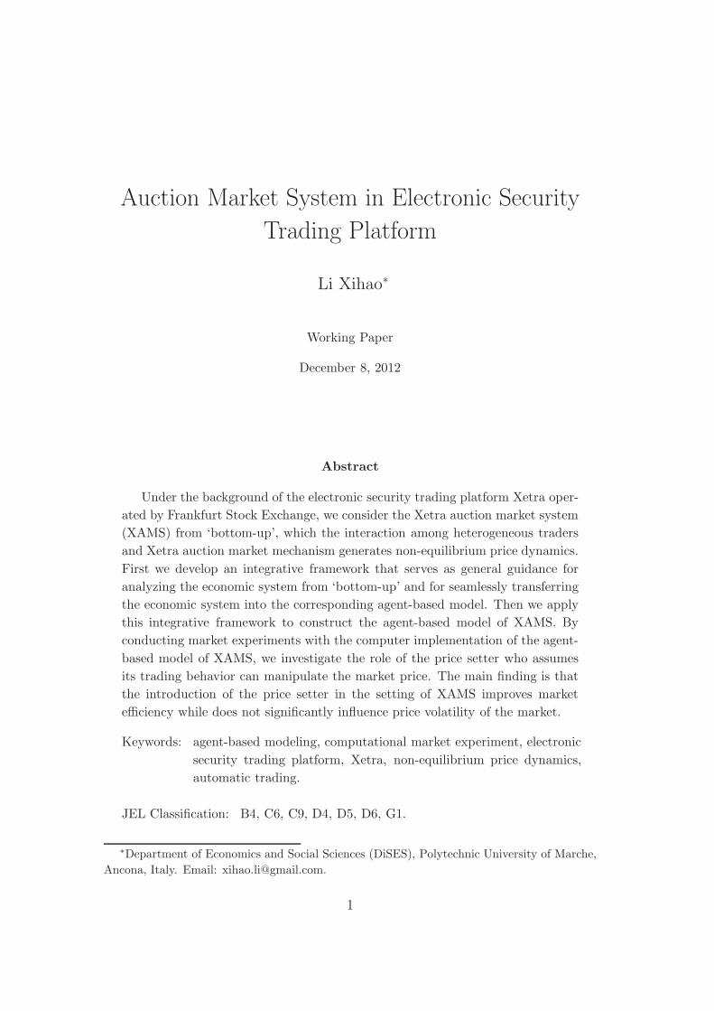
In general, we follow the ACE modeling procedure that is depicted in Figure 1.
First, by applying the Agent-Based Modeling (ABM) method which considers
modeling the system as a collection of interacting agents, the ACE modeler an-
alyzes the economic system and constructs the corresponding ACE model which
is an abstracted representation of the economic system. Then the ACE modeler
employs computer programming languages to implement the ACE model as the
computer software system. After that, the ACE modeler initiates and executes
the software system to observe in the computer environment the evolution of the
software system which represents the dynamics of the economic system.
4
Page 6
EconomicSystem
Agent-BasedModeling
ACEModel
SoftwareSystem
ComputerProgramming
Language
Figure 1: The ACE modeling procedure.
As stated in (LeBaron, 2006), the current difficulty of constructing agent-based
models for economic systems is the lack of general principles that economists
can refer to when constructing agent-based models to represent economic sys-
tems. In this work, we aim at providing an integrative framework that serves as
general guidance for analyzing economic systems from ‘bottom-up’ and for seam-
lessly transferring economic systems into agent-based models. We start from
the perspective of systems theory and the methodology of ABM to investigate
an economic system from ‘bottom-up’ and to derive constructive aspects of the
economic system which serve as the foundation of the integrative framework for
ACE modeling.
2.1 Constructive Aspects of Economic System
Constructive aspects of economic system have the epistemic root in the system-
atic principle of economic phenomena and processes, i.e. economic phenomena
and processes can be regarded as states and evolutionary processes of the corre-
sponding economic systems.1
From systems theory and the methodology of ABM, an economic system from
‘bottom-up’ can be regarded as a dynamical open system which interacts with its
surrounding or environment in the society. An economic system is a collection
1The systematic principle of economic phenomena and processes is the specification of the
systems theory in the field of economics, see (Bertalanffy, 1993).
5
Page 7
of economic entities (consumers, firms, commodities, markets, etc.) interacting
with each other such that the interactions of economic entities perform macro-
scopic behavior of the system given the influence from the environment. From
this understanding on economic systems, we extract four aspects, denoted as
constructive aspects of economic system, that require to be specified to
construct an economic system from ‘bottom-up’.
I. The scope of the economic system and its environment;
II. The interrelation between the economic system and its environment;
III. Elements of the economic system, which are economic entities considered
in the economic system;
IV. The structure of the economic system, which is the interrelation among
elements of the economic system.
To model an economic system, constructive aspects of economic system suggest
to formulate aspect I to IV of the economic system and their updating rules
(also called state transition rules) which represent the dynamics of the economic
system.
Economists normally specify the scope of the economic system and its environ-
ment when initiating their economic research. Consider the composite of the
economic system and its environment as the economic world and regard the inter-
relation between the economic system and its environment as information flows.2
Then one obtains the ACE world which integrates the ACE model of the economic
system and its environment with the information flows.
As observed in contemporary economic literature, economists tend to classify
economic entities into different types in order to investigate the characteristics
of each type. For example, (Pindyck & Rubinfeld, 2001) clusters microeconomic
entities into consumers, producers (firms), commodities, markets, etc. In prin-
ciple, this classification of economic entities regulates elements in the economic
system and the corresponding agents in the ACE model.
The structure of the economic system represents the information flows among
agents in the ACE model. One possibility to explicitly depict in the ACE model
the structure of the economic system is to apply the mathematical concept of
2The concept of information can be termed as diversified meanings. Here the information
is considered as quantitative representations of the economic world. Knowledge, methods, and
actions are regarded as information in this sense once they can be quantified.
6
Page 8
graph. We develop the diagram of the relationship for the ACE model which
nodes represent agents in the ACE model and which arcs visualize information
flows between agents.3 The diagram of the relationship visualizes the interrelation
between the economic system and its environment as the arcs which connect the
corresponding ACE model with its environment.
Now the crucial point is to model economic entities with the concept of agents.
Most economic entities investigated in economic research are concerned with the
functionality and behavior of individual or a group of people in economic world.
We denote all these economic entities interpreting the functionality of human
subject as active economic entities in the sense that they behave actively
to fulfill their needs and objectives. Economic entities which are not directly
involved with the functionality of human subject, e.g. commodities traded in
the markets, are classified as passive economic entities. Correspondingly, we
denote the agent representing the active economic entity as the active economic
agent and the agent representing the passive economic entity as the passive
economic agent.
An economic system can be treated as an economic entity that is used to con-
struct another economic system, whereas an element in the economic system can
be treated as an economic system. This property of system-element duality guar-
antees the hierarchy of economic systems, see (Potts, 2000). More importantly,
this property infers that one can consider the economic entity as a collection of
components whose interaction among each other provides the functionality of the
economic entity and thus one can model the economic entity by formulating its
constructive aspects.
2.2 Constructive Aspects of Active Economic Entity
In economic literature, active economic entities represent the functionality of
decision makers in the economic world. The concept of the decision maker has
been investigated in various fields in science which include psychology, sociology,
computer science, etc. As we are looking for the general framework to construct
the ACE model that is to be implemented as computer software system, we
employ the related concepts in computer science and combine with decision theory
3The diagram of the relationship for the ACE model serves the same purpose as the class
diagram which describes the static structure of objects in a system and their relationships
in Unified Modeling Language (UML), see (Blaha & Rumbaugh, 2004). Comparing with the
class diagram in UML, the diagram of the relationship for the ACE model emphasizes on the
connections of information flows among agents.
7
Page 9
in economics to model the active economic entity.
The skeleton of the decision maker is stated in the concept of the agent in arti-
ficial intelligence (AI), a subfield of computer science. An agent in this field is
“anything that can be viewed as perceiving its environment through sensors and
acting upon that environment through actuators” (Russell & Norvig, 2003, p. 32).
Following this line, we develop a general pattern by integrating behavioral rules of
active economic entities investigated in economic research with the current con-
cept of the learning agent in AI, see (p. 53, ibid.). This general pattern, called
the module of active economic agent (MAEA), is regarded as construc-
tive aspects of the active economic entity and is composed of the submodule of
information acquirement, the submodule of storage, the submodule of learning,
the submodule of objectives, the submodule of forecasting, and the submodule of
action transmission. One applies MAEA to construct the corresponding active
economic agent from ‘bottom-up’ by specifying its submodules and the interre-
lation among submodules. We sketch the functionality of each submodule with
the structure of MAEA illustrated in Figure 2.
Figure 2: The structure of MAEA.
The environment in Figure 2 represents those parts that are out of the scope
of the active economic agent. The information flows between MAEA and the
8
Page 10
environment represent the interrelation of the agent with others in the economic
system.
The submodule of information acquirement establishes the connections with its
environment and collects information through the interrelations. The submodule
of storage stores the information about the state of the agent. It collects the
information transmitted from other submodules and sends out the information on
request. The submodule of forecasting generates the forecast on uncertain factors
that the agent considers. The submodule of objectives depicts the objectives
that the agent intends to achieve, selects the action plan based on its designated
objectives, and sends out the action plan to the submodule of action transmission
to realize the action. The submodule of action transmission receives action plans
from the submodule of objectives and realizes the action through its interrelations
with the environment. The submodule of learning considers the learning process
of the agent, which might not be constructed as it is not a compulsory piece when
modeling the agent in economic literature.
The state of the active economic agent evolves when the agent acts to fulfill its
objectives. The updating rules of the agent are thus the decision making process
that is presented by interactions among submodules.
The decision making process generally starts when the agent initiates its state.
The agent observes information via the submodule of information acquirement
and keeps the information in its memory via the submodule of storage. Then it
applies the submodule of learning to update itself, e.g. to update the forecasting
methods currently applied in the submodule of forecasting in order to provide
more accurate forecast on uncertain factors that the agent considers. After that,
the agent generates its subjective forecast via the submodule of forecasting, se-
lects the action plan to fulfill its objectives via the submodule of objectives,
and transmits the action to the economic system via the submodule of action
transmission. Finally, the agent receives from the environment the feedback of
its action. This general decision making process is illustrated in Figure 3 and
is worked as a benchmark for depicting the updating rules of active economic
agents.
2.3 Constructive Aspects of Passive Economic Entity
Passive economic entities do not behave actively to fulfill their objectives. They
mainly act as information providers that disseminate information to active eco-
nomic entities on request. We propose a general pattern named the module
of passive economic agent (MPEA) to construct passive economic agents.
9
Page 11
Figure 3: The general decision making process of active economic agent.
MPEA consists of a set of economic properties that represent the informa-
tion considered in the agent and associated operations such as the operation of
information update that is regarded as the updating rules of the agent.
2.4 Integrative Framework for ACE Modeling
The integrative framework for ACE modeling is a modeling process that applies
the constructive aspects of the economic system and of the economic entities to
translate the economic system into the corresponding ACE model. Given the
economic system in study, the integrative framework starts with specifying con-
structive aspects of the economic system. Then it applies MAEA and MPEA
as templates to formulate the corresponding economic agents in the economic
system. It models the updating rules of active economic agents with the decision
making process and the updating rules of passive economic agents with the op-
eration of information update. The updating rules of economic agents constitute
the updating rules of the ACE model. Given information flows between the ACE
model and its environment, the interactions among agents generate the dynamics
of the model.
10
Page 12
To explicitly present the dynamic process generated by the interactions among
agents in the ACE model, we assign in the form of the flowchart the diagram
of the interaction for the ACE model to describe the sequence of work-flows
and activities among agents.4 In summary, the integrative framework contains
the modeling procedure as follows:
1. Specify constructive aspects of the economic system;
2. Construct corresponding agents in the ACE model by applying MAEA and
MPEA respectively, model the decision making process of active economic
agents and the operation of information update in passive economic agents;
3. Present the diagram of the interaction to describe the sequence of workflows
and activities among agents for the dynamics of the ACE model.
3 ACE Model of Xetra Auction Market System
We apply the integrative framework to construct the ACE model of XAMS.
Consider an economic world with one risky asset market and one risk-free asset
market in trading period t ∈ {1, . . . , T}. The economic world applies Euro (e) as
the trading currency. The risky asset considered in the market has no dividend
and is traded in integer shares, i.e. traders can trade 19 shares of the risky asset
but not 19.81 shares. The risk-free asset is divisible in any trading quantity with
the trading price normalized to 1. It has a constant interest factor R which can
be interpreted as 1 + r with r denoting the nominal interest rate. N traders
participate in the economic world to trade in the risky asset market and the risk-
free asset market. The economic world has no transaction cost and no short sale
constraint for traders.
The risky asset market is a Xetra auction market that holds one Xetra auction
for each trading period to determine the market price and the trading volume
by XAMM. Xetra auction consists of the call phase and the price determination
phase. During the call phase, XAMM disseminates the real-time trading data
of the central order book in the market. Upon observing the real-time trading
data from the market, traders perform their investment decisions and submit
orders. XAMM then collects the submitted orders to the central order book and
4The diagram of the interaction serves as the flowchart version of the activity diagram
in Unified Modeling Language (UML) which is to represent the sequence of activities among
components in the system, see (Blaha & Rumbaugh, 2004).
11
Page 13
simultaneously updates the real-time trading data. The call phase stops randomly
after a fixed time span and the price determination phase follows to determine
Xetra auction price and the final transaction volumes. After that, XAMM cancels
the unexecuted part of the orders and conducts the settlement to complete the
payment for each transaction. After trading in Xetra auction market, traders
interact with the risk-free asset market and trade for the risk-free asset.
We focus on Xetra auction market and regard the risk-free asset market as the
environment of Xetra auction market. Given the information flows from the
risk-free asset market, the interactions among traders and XAMM provide the
functionality of Xetra auction market, i.e. determining the trading price and
reallocating the risky asset among traders. We apply the integrative framework
to construct the ACE model of XAMS. The first step is to consider constructive
aspects of XAMS.
Example 1 (Constructive aspects of XAMS).
I. XAMS considers economic entities which operate in the market, i.e. N
traders, XAMM, the numeraire employed in the market, and the risky asset
traded in the market. The environment of XAMS is the risk-free asset market.
II. XAMS connects to the risk-free asset market to request the information
of the interest factor R as well as to transmit trader’s trading request on the
risk-free asset. The risk-free asset market connects to XAMS to inform traders
the interest factor R as well as their realized trading quantities of the risk-free
asset. These information flows represent the interrelation between XAMS and
its environment.
III. XAMS is regarded as a dynamical system which implicitly contains the
concept of time. We apply the concept of the system clock to represent the
time horizon considered in the ACE model. Thus, elements of XAMS as well
as the corresponding ACE model are: N traders, XAMM, the numeraire, the
risky asset, and the system clock.
IV. Consider a decentralized market. Traders connect with XAMM in order
to perform the trading behavior, whereas there is no direct connection among
traders. Traders and XAMM connect to the numeraire, the risky asset, and
the system clock to have access to the associated information. Denote Xetra
auction market center in the ACE model as a composite of XAMM, the nu-
meraire, the risky asset, and the system clock. Then the structure of XAMS
follows the type of the star network, see Figure 4. Xetra auction market center
12
Page 14
as the central node in the star network connects with all other nodes of traders
in the ACE model.
……
……
..…...
Risky
AssetXAMM
System
Clock
Numeraire
Figure 4: The diagram of the relationship for the ACE model of XAMS.
Classify agents in XAMS as active economic agents of N traders and XAMM with
passive economic agents of the numeraire, the risky asset, and the system clock.
The second step of the integrative framework is to apply MAEA and MPEA to
construct these agents respectively.
We consider three types of traders in XAMS. The first type is the price setter who
assumes that, with the knowledge on XAMM and the real-time trading data, it
could manipulate the current trading price as well as its transaction volume by its
trading behavior. The second type is the price taker who believes that its trading
behavior has no impact on the market. The last type is the noise trader who is
assumed to act randomly in the market. Assume trader 1 in the ACE model as
the price setter, trader j ∈ {2, . . . , N − 1} as price takers, and trader N as the
noise trader. For simplicity, further assume that each trader submits at most one
order in each trading period with price setter and noise trader submitting the
13
Page 15
market order and price takers submitting the limit order. We apply MAEA to
construct trader 1 in Example 2, trader j ∈ {2, . . . , N − 1} in Example 3, and
trader N in Example 4 respectively.
Example 2 (Trader 1). As stated in Figure 4, trader 1 connects with Xetra
auction market center and the risk-free asset market. At the beginning of the
trading period t, trader 1 is with the initial endowment (y(1)0 [t], Z
(1)0 [t]) where
y(1)0 [t] is the initial holding of the risk-free asset and Z
(1)0 [t] is the initial holding
of the risky asset. Trader 1 obtains through its submodule of information ac-
quirement the interest factor R from the risk-free asset market and the real-time
data set I0[t] of the central order book from XAMM.
By applying the submodule of forecasting, trader 1 computes the expected mean
value qe(1)[t] of the risky asset price for the next trading period t+1 and its asso-
ciated variance V e(1)[t]. As trader 1 can manipulate the current trading price as
well as its transaction volume by submitting its market order, it performs its sub-
jective forecast Pe(1)X [t](Qm) on the current Xetra auction price and Z
e(1)X [t](Qm)
on the final transaction volume for period t which are functions with the control
variable Qm of the quoted trading quantity in its market order. The values of
Pe(1)X [t](Qm) and Z
e(1)X [t](Qm) are the trading price and the final transaction vol-
ume that XAMM would calculate by perceiving the trader’s market order with
quoted trading quantity Qm would be added to the current central order book in
the market.
With its forecast of {Pe(1)X [t](Qm), Z
e(1)X [t](Qm), q
e(1)[t], V e(1)[t]}, the trader has
the budget constraint:
Pe(1)X [t](Qm) · Z
e(1)X [t](Qm) + ye(1)[t] = 0, (1)
where ye(1)[t] is the trader’s expected trading quantity of the risk-free asset in
period t. The trader expects the portfolio holding after trading in period t as
(y(1)0 [t] + ye(1)[t], Z
(1)0 [t] + Z
e(1)X [t](Qm)). Complying with the budget constraint
(1), the trader considers the mean value mean(1)[t] of its future wealth at the end
of the trading period t as:
mean(1)[t] = {qe(1)[t]− R · Pe(1)X [t](Qm)} · Z
e(1)X [t](Qm)
+qe(1)[t] · Z(1)0 [t] +Ry
(1)0 [t]. (2)
The associated variance var(1)[t] is as:
var(1)[t] = {Z(1)0 [t] + Z
e(1)X [t](Qm)}
2 · V e(1)[t]. (3)
14
Page 16
We assume that trader 1 takes the linear mean-variance preference. The trader
presents its objective in the submodule of objectives as the portfolio selection
problem:
maxQm∈Z
mean(1)[t]−α1
2var(1)[t] (4)
⇔ maxQm∈Z
{qe(1)[t]− R · Pe(1)X [t](Qm)} · Z
e(1)X [t](Qm)
+qe(1)[t] · Z(1)0 [t] +Ry
(1)0 [t]−
α1
2{Z
(1)0 [t] + Z
e(1)X [t](Qm)}
2 · V e(1)[t],
where α1 is a constant measure of absolute risk aversion. Trader 1 solves this
portfolio selection problem (4) and obtains the integer maximizer Q(1)m [t] with
Q(1)m [t] > 0 denoting the trading quantity on the demand side and Q
(1)m [t] <
0 denoting the trading quantity on the supply side. Then the trader submits
the market order with the quoted trading quantity Q(1)m [t] to XAMM via the
submodule of action transmission.
Trader 1 realizes the trading price PX [t] and its transaction volume Z(1)X [t] after
XAMM determines the trading price and the trading volume in the price deter-
mination phase. Then the trader completes with XAMM the payment for its
transaction.
After trading the risky asset, trader 1 attains from the risk-free asset market the
share y(1)[t] = −PX [t] · Z(1)X [t] of the risk-free asset. The portfolio holding that
the trader acquires after trading in period t is (y(1)0 [t] + y(1)[t], Z
(1)0 [t] + Z
(1)X [t])
and the trader’s initial endowment of the next trading period t+ 1 is
{
y(1)0 [t+ 1] = R(y
(1)0 [t] + y(1)[t]),
Z(1)0 [t+ 1] = Z
(1)0 [t] + Z
(1)X [t].
(5)
The decision making process of trader 1 is illustrated in Figure 5.
Example 3 (Trader j = 2, . . . ,N− 1). Analogous to trader 1, trader j connects
with Xetra auction market center and the risk-free asset market. At the beginning
of the trading period t, trader j is with the initial endowment (y(j)0 [t], Z
(j)0 [t]). The
trader obtains through its submodule of information acquirement the interest
factor R and the real-time order book data set I0[t].
By applying the submodule of forecasting, trader j computes the expected mean
value qe(j)[t] of the risky asset price for the next trading period t + 1 and its
associated variance V e(j)[t]. As the trader has to decide a limit price to quote in
its limit order, the trader conducts its subjective forecast Pe(j)X [t] on the current
15
Page 17
Collect information via the interrelation
START
END
Store information in the trader’s memory
Generate initial state
Trade for of the risk-free asset from
the risk-free asset market
][)1(
ty
Complete the payment for the transaction
Select the optimal market order to
maximize the trader’s expected utility on the
mean-variance preference
][)1(
tQm
Realize the final transaction volume
with the trading price][)1(
tZ X ][tPX
Forecast the expected mean value ,
the associated variance , the expected
Xetra auction price function ,
and the expected Xetra auction allocation
function
][)1(
tqe
)]([)1(
meX QtZ
)]([)1(
meX QtP][
)1(tV
e
Submit the optimal market order ][)1(
tQ m
Figure 5: The decision making process of trader 1 in Example 2.
Xetra auction price and regards its forecast as the limit price. The trader expects
it will realize from the market the quoted trading quantity Ql in its limit order.
With its forecast of {qe(j)[t], V e(j)[t], Pe(j)X [t]}, the trader has the budget con-
straint:
Pe(j)X [t] ·Ql + ye(j)[t] = 0, (6)
where ye(j)[t] is the trader’s expected trading quantity of the risk-free asset in
period t. The trader expects the portfolio holding after trading in period t as
(y(j)0 [t] + ye(j)[t], Z
(j)0 [t] + Ql). Complying with the budget constraint (6), the
trader considers the mean value mean(j)[t] of its future wealth at the end of the
16
Page 18
trading period t as:
mean(j)[t] = {qe(j)[t]−R · Pe(j)X [t]} ·Ql + qe(j)[t] · Z
(j)0 [t] +Ry
(j)0 [t]. (7)
The associated variance var(j)[t] is as:
var(j)[t] = {Z(j)0 [t] +Ql}
2 · V e(j)[t]. (8)
Assume that trader j takes the linear mean-variance preference. The trader
presents its objective in the submodule of objectives as the portfolio selection
problem:
maxQl∈Z
mean(j)[t]−αj
2var(j)[t] (9)
⇔ maxQl∈Z
{qe(j)[t]− R · Pe(j)X [t]} ·Ql
+ qe(j)[t] · Z(j)0 [t] +Ry
(j)0 [t]−
αj
2{Z
(j)0 [t] +Ql}
2 · V e(j)[t],
where αj is a constant measure of absolute risk aversion. Trader j solves this
portfolio selection problem (9) and obtains the integer maximizer Q(j)l [t]. Then
the trader submits its limit order with the price-quantity pair (Pe(j)X [t], Q
(j)l [t]) to
XAMM via the submodule of action transmission.
Trader j realizes the trading price PX [t] and its transaction volume Z(j)X [t] after
XAMM determines the trading price and the trading volume in the price deter-
mination phase. Then the trader completes with XAMM the payment for its
transaction.
After trading the risky asset, trader j attains from the risk-free asset market the
share of risk-free asset y(j)[t] = −PX [t] · Z(j)X [t]. The portfolio holding that the
trader acquires after trading in period t is (y(j)0 [t] + y(j)[t], Z
(j)0 [t] + Z
(j)X [t]) and
the trader’s initial endowment of the next trading period t + 1 is
{
y(j)0 [t + 1] = R(y
(j)0 [t] + y(j)[t]),
Z(j)0 [t+ 1] = Z
(j)0 [t] + Z
(j)X [t].
(10)
The decision making process of trader j is illustrated in Figure 6.
Example 4 (Trader N). Consider trader N is with the initial endowment of
(y(N)0 [t], Z
(N)0 [t]) at the beginning of the trading period t. Trader N obtains the
interest factor R from the risk-free asset market.
17
Page 19
Collect information via the interrelation
START
END
Store information in the trader’s memory
Generate initial state
Complete the payment for the transaction
Trade for of the risk-free asset from
the risk-free asset market
][)(
tyj
Forecast the expected mean value ,
the associated variance , and the
expected Xetra auction price
][)(
tqje
][)(
tPje
X
][)(
tVje
Submit the optimal limit order
])[],[()()(
tQtPj
lje
X
Select the optimal limit order
to maximize the trader’s
expected utility ])[],[(
)()(tQtP
jl
jeX
Realize the final transaction volume
with the trading price][)(
tZj
X][tPX
Figure 6: The decision making process of trader j in Example 3.
The trader randomly selects Q(N)m [t] from the set Qrange of all possible trading
quantities considered by the noise trader. Then the trader constructs its market
order with the quoted trading quantity Q(N)m [t] and submits the order to XAMM.
Trader N realizes the trading price PX [t] and its transaction volume Z(N)X [t] after
XAMM determines the trading price and the trading volume in the price deter-
mination phase. Then the trader completes with XAMM the payment for its
transaction.
After trading the risky asset, trader N attains from the risk-free asset market the
18
Page 20
shares of the risk-free asset y(N)[t] = −PX [t] · Z(N)X [t]. The portfolio holding that
the trader acquires after trading in period t is (y(N)0 [t] + y(N)[t], Z
(N)0 [t] +Z
(N)X [t])
and the trader’s initial endowment for the next trading period t+ 1 is
{
y(N)0 [t+ 1] = R(y
(N)0 [t] + y(N)[t]),
Z(N)0 [t+ 1] = Z
(N)0 [t] + Z
(N)X [t].
(11)
The decision making process of trader N is illustrated in Figure 7.
Collect information via the interrelation
START
END
Store information in the trader’s memory
Generate initial state
Complete the payment for the transaction
Trade for of the risk-free asset from the risk-free asset market
][)(
tyN
Select the market order randomly][)(
tQN
m
Realize the final transaction volume with the trading price][
)(tZ
NX ][tPX
Submit the market order ][)(
tQN
m
Figure 7: The decision making process of trader N in Example 4.
XAMM is another type of active economic agent considered in the ACE model.
Its objective is to determine Xetra auction price and the final transaction volume
according to the central order book.
19
Page 21
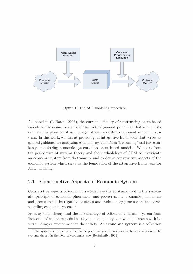
Example 5 (XAMM). At the beginning of the trading period t, XAMM has his-
torical trading prices PX [i] for trading period i ∈ {−KXAMM +1, . . . , 0} with the
memory span KXAMM > 0. It contains trading information (I0[i], PX [i], ZX [i])
for trading period i ∈ {1, . . . , t − 1} where I0[i] is the order book data set
at the end of the call phase, PX [i] is the Xetra auction price, and ZX [i] =
{Z(1)X [i], . . . , Z
(N)X [i]} is the collection of the final transaction volume Z
(j)X [i] for
each trader j ∈ {1, . . . , N}. In summary, XAMM at the beginning of the trading
period t is with the historical trading information set
Infor[t− 1] ={
(I0[t− 1], PX [t− 1], ZX [t− 1]), . . . , (I0[1], PX [1], ZX[1]),
PX [0], . . . , PX [−KXAMM + 1]}
. (12)
During the call phase, XAMM works through the submodule of information ac-
quirement to collect order specifications {Q(1)m [t], . . . , (P
e(j)X [t], Q
(j)l [t]), . . . , Q
(N)m [t]}
submitted by traders and stores this information via the submodule of storage.
It simultaneously disseminates the real-time order book data set I0[t].
The objective of XAMM is to determine in the price determination phase the
Xetra auction price PX [t] and the final transaction volumes ZX [t] = {Z(1)X [t], . . . ,
Z(N)X [t]} by applying Xetra auction trading rules stated in (Gruppe Deutsche
Borse, 2003), see the formulation in Appendix A. After determining Xetra auc-
tion price and the trading volume, XAMM cancels the unexecuted part of order
specifications and conducts the settlement process to complete the payment for
each transaction. Then XAMM closes the market until the next trading period
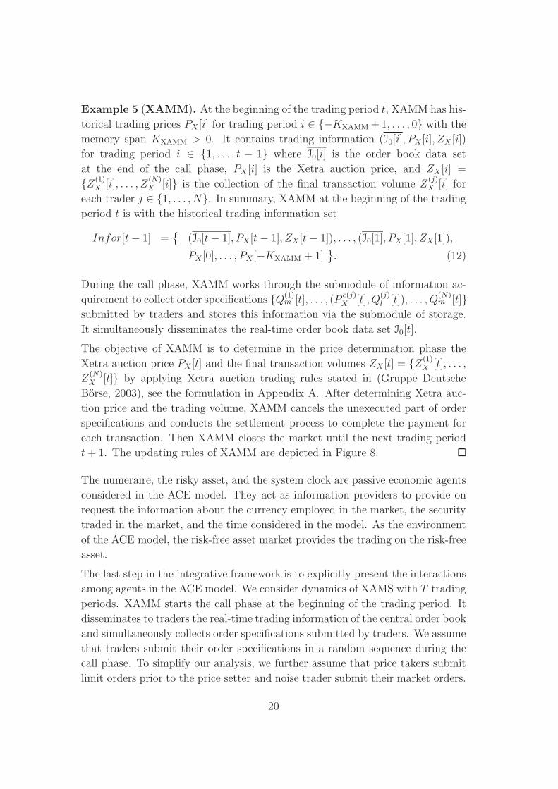
t+ 1. The updating rules of XAMM are depicted in Figure 8.
The numeraire, the risky asset, and the system clock are passive economic agents
considered in the ACE model. They act as information providers to provide on
request the information about the currency employed in the market, the security
traded in the market, and the time considered in the model. As the environment
of the ACE model, the risk-free asset market provides the trading on the risk-free
asset.
The last step in the integrative framework is to explicitly present the interactions
among agents in the ACE model. We consider dynamics of XAMS with T trading
periods. XAMM starts the call phase at the beginning of the trading period. It
disseminates to traders the real-time trading information of the central order book
and simultaneously collects order specifications submitted by traders. We assume
that traders submit their order specifications in a random sequence during the
call phase. To simplify our analysis, we further assume that price takers submit
limit orders prior to the price setter and noise trader submit their market orders.
20
Page 22
START
END
Time to end the call phase?
yes
no
End the trading period
Start the trading period
The price determination phase: compute the
trading price and the final transaction volume, send out the trading information, cancel the
unexecuted part of the order specifications
The settlement process: conduct the payment
process for transactions among traders
The call phase: disseminate the real-time trading information, collect the order
specifications
Figure 8: The updating rules of XAMM.
The call phase stops randomly after a fixed time span and is followed by the
price determination phase. XAMM determines in the price determination phase
the Xetra auction price and the final transaction volume. Then it cancels the
unexecuted part of the orders and conducts the settlement process to complete
the payment for each transaction. After trading in the Xetra auction market,
traders obtain the risk-free asset holdings via the interaction with the risk-free
asset market. XAMS iterates to the next trading period until it reaches the last
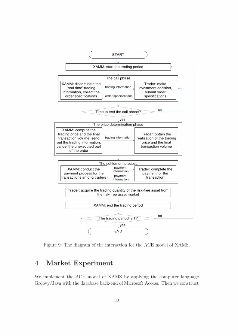
trading period T . The diagram of the interaction in Figure 9 explicitly illustrates
the work-flows of activities among agents in the market dynamics.
21
Page 23
START
END
Time to end the call phase?
yes
no
XAMM: end the trading period
Trader: acquire the trading quantity of the risk-free asset from the risk-free asset market
The trading period is T?
XAMM: start the trading period
no
yes
The call phase
XAMM: disseminate the ‘real-time’ trading
information, collect the order specifications
Trader: make investment decision,
submit order specifications
trading information
order specifications
The price determination phase
XAMM: compute the trading price and the final transaction volume, send
out the trading information, cancel the unexecuted part
of the order
Trader: obtain the realization of the trading
price and the final transaction volume
trading information
The settlement process
XAMM: conduct the payment process for the
transactions among traders
Trader: complete the payment for the
transaction
payment
information
payment
information
Figure 9: The diagram of the interaction for the ACE model of XAMS.
4 Market Experiment
We implement the ACE model of XAMS by applying the computer language
Groovy/Java with the database back-end of Microsoft Access. Then we construct
22
Page 24
the market experiment and conduct the computer simulation of XAMS. The focus
of the market experiment is on the generated dynamics of Xetra auction price.
Specifically, we are concerned with:
1. whether the generated Xetra auction price is generically non market-clearing.
2. the impact of the price setter on the non market-clearing property and on the
volatility of the Xetra auction price in the market.
4.1 Experimental Setup
We setup the simulation profile for the Xetra auction market experiment by
initializing the parameters and by specifying the forecasting methods employed
by agents.
Model’s Parameters to Initialize
• T = 250 . . . time horizon. The time horizon approximates the time span of one
year when considering one auction for each trading day and 255 trading days
for Frankfurt Stock Exchange in the year of 2009.
• N = 22 . . . number of traders. Three types of traders are considered in the
model with 1 price setter, 20 price takers, and 1 noise trader.
• r . . . the interest rate of the risk-free asset. The interest rate is assumed to be
constant in each profile. According to the Eurostat5, the 3-months interest rate
in European Union (27 countries) for the period of October 2008 to September
2009 is in the range of [1.04%, 5.52%]. We choose r randomly from this range.
XAMM’s Parameters to Initialize
• {PX [0], . . . , PX [−KXAMM + 1]} . . . the historical trading prices. We consider
PX [0], . . . , PX [−KXAMM+1] as historical auction prices of the stock “Deutsche
Borse AG” listed in Xetra for the period from August 27, 2009 to November
04, 2009, with the memory span KXAMM = 100.6
5See http://epp.eurostat.ec.europa.eu.6This historical data of the stock trading price is provided online by Deutsche Borse, see
http://deutsche-boerse.com.
23
Page 25
• rangep = 10% . . . the percentage of the price range. The Xetra platform re-
quires transactions executed under certain price range from the last traded
price Pref . While it does not publicly provide the information of the per-
centage of the price range, another electronic trading platform Euronext re-
quires the percentage of ±10%. We employ the setting in Euronext and choose
rangep = 10%. Thus, XAMM considers Xetra auction price in the range of
[Pref(1− 10%), Pref(1 + 10%)].
Trader’s Parameters to Initialize
• y(j)0 [1] . . . trader j’s initial risk-free asset holding at the beginning of the trading
period 1. We take y(j)0 [1] as a random positive number.
• Z(j)0 [1] . . . trader j’s initial risky asset holding at the beginning of the trading
period 1. We take Z(j)0 [1] as a random integer number. To simplify the anal-
ysis, we assume that the aggregated volume in the market is constant with∑22
j=1Z(j)0 [1] = 1000.
• α(j) . . . the measure of absolute risk aversion in the trader’s utility function
with the linear mean-variance preference. α(j) is assumed to be constant in
each profile and is selected randomly from the range of (0, 2].
• Qrange . . . the set of the trading behavior for the noise trader j = 22 depicted
in Example 4.
We assume that the noise trader randomly chooses for each trading period the
trading behavior from the set of Qrange = { selling 1 unit, buying 1 unit }.
We keep the noise trader’s random choice of trading behavior for each period
the same in the benchmark market experiment as in the Xetra auction market
experiment.
Trader’s Forecasting Methods to Initialize
1. Forecasting Methods in Common
For each period t, trader j = 1 depicted in Example 2 and price takers j ∈
{2, . . . , 21} depicted in Example 3 compute the expected mean value qe(j)[t]
of the risky asset price for the next trading period t + 1 and its associated
variance V e(j)[t]. We assume two types of forecasting: the fundamentalist and
the chartist. The forecasting type remains unchanged in each profile after
trader j randomly chooses the forecasting type with equal probability.
24
Page 26
(a) The Fundamentalist
• qe(j)[t] . . . The fundamentalist believes the mean value and the asso-
ciated variance of the market price remain unchanged. It computes
qe(j)[t] as the mean value of the historical trading prices PX [0], . . . ,
PX [−KXAMM + 1] with
qe(j)[t] =1
KXAMM
KXAMM∑
n=1
PX [1− n].
• V e(j)[t] . . . The fundamentalist computes V e(j)[t] as the associated
variance of the historical trading prices PX [0], . . . , PX [−KXAMM + 1]
with
V e(j)[t] =1
KXAMM − 1
KXAMM∑
n=1
(PX [1− n]− qe(j)[t])2.
The fundamentalist has constant forecast of qe(j)[t] and V e(j)[t] for each
trading period.
(b) The Chartist
• qe(j)[t] . . . The chartist expects the trend of the price movement based
on the historical price movement. There are two types of chartists
in our simulation: the trend follower and the contrarian. The trend
follower expects the trading price will increase (decrease) given the
trading price increased (decreased) in the last trading period while
the contrarian expects the opposite. Let the indicator idc = 1 for
trend follower and idc = −1 for contrarian. With historical trading
prices PX [t−1] and PX [t−2], the forecasting of the chartist at period
t is
qe(j)[t] =
PX [t− 1](1 + idc · ω(j)) if PX [t− 1] > PX [t− 2],
PX [t− 1] if PX [t− 1] = PX [t− 2],
PX [t− 1](1− idc · ω(j)) if PX [t− 1] < PX [t− 2];
where ω(j) measures how aggressive of the price movement that the
trader expects.
idc and ω(j) are assumed to be constant after idc is chosen randomly
from {−1, 1} with equal probability and ω(j) is chosen randomly from
the range of (0, rangep].
25
Page 27
• V e(j)[t] . . . It is assumed that the chartist keeps V e(j)[t] constant in
the profile after it is chosen randomly from the range (0, 5].
2. Forecasting Method for Price Setter j = 1 depicted in Example 2
• Pe(1)X [t] . . . the forecast on Xetra auction price in the current trading pe-
riod t. By applying formulation (16) in Appendix B, the price setter
computes the forecast Pe(1)X [t](Q
(1)m [t]) that is a function of the quoted
trading quantity Q(1)m [t] in its market order.
• Ze(1)X [t] . . . the forecast on the trader’s final transaction volume in the
current trading period t. By applying formulation (17) in Appendix B,
the price setter computes Ze(1)X [t](Q
(1)m [t]) that is a function of the quoted
trading quantity Q(1)m [t] in its market order.
3. Forecasting Method for Price Taker j = 2, . . . , 21 depicted in Example 3
• Pe(j)X [t] . . . the forecast on Xetra auction price in the current trading period
t. It is assumed that Pe(j)X [t] is randomly chosen from the price range
[Pref(1− 10%), Pref(1 + 10%)] stipulated in XAMM.
4.2 Experimental Procedure
To investigate the market dynamics and the impact of the price setter in Xetra
auction market, we construct along with the Xetra auction market experiment
a benchmark market experiment. The benchmark market experiment has the
same setup as the Xetra auction market experiment except for the price setter
j = 1 depicted in Example 2. The benchmark market experiment replaces the
price setter j = 1 with the benchmark trader which follows the same setup as
depicted in Example 2 except for adopting the forecast Ze(1)X [t](Qm) = Qm and
Pe(1)X [t](Qm) = Pref where Pref is the last traded price in Xetra auction market.
Thus, the benchmark trader considers its objective in the submodule of objectives
as the portfolio selection problem:
maxQm∈Z
{qe(1)[t]− R · Pref} ·Qm + qe(1)[t] · Z(1)0 [t] +Ry
(1)0 [t]
−α1
2{Z
(1)0 [t] +Qm}
2 · V e(1)[t], (13)
where α1 is a constant measure of absolute risk aversion. As observed in (13), the
trader considers in its portfolio selection problem that the current trading price
and the trader’s final trading volume are independent of Qm. The benchmark
26
Page 28
trader is thus regressed to a price taker who has no manipulation on the current
trading price and on the trading volume by its market order.
We consider 50 rounds of market experiments. It starts with initiating 50 sim-
ulation profiles for each round of the market experiment with the index s ∈
{1, . . . , 50}. Then for each profile s, we conduct the benchmark market exper-
iment and the Xetra auction market experiment with 250 trading periods of
simulations.
4.3 Experimental Results
0 50 100 150 200 250
050
100
150
200
period
price
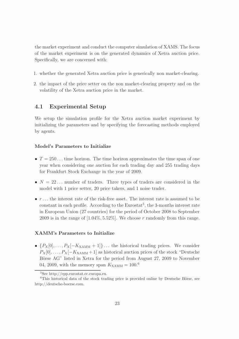
Figure 10: The price dynamics in 50 profiles.
Price Dynamics. We consider the price dynamics for 250 trading periods gen-
erated in the market experiment. Figure 10 illustrates the price dynamics gener-
ated by all 50 simulation profiles. The blue color in this figure as well as in the
following figures is for the benchmark market experiment and the red color is for
the Xetra auction market experiment.
Figure 10 demonstrates the divergence of the price dynamics in the market ex-
periment. Consider the end-of-period trading price as the market price in the
27
Page 29
benchmark market
price
frequ
ency
0 50 100 200
02
46
810
12Xetra auction market
price
frequ
ency
0 50 100 2000
24
68
1012
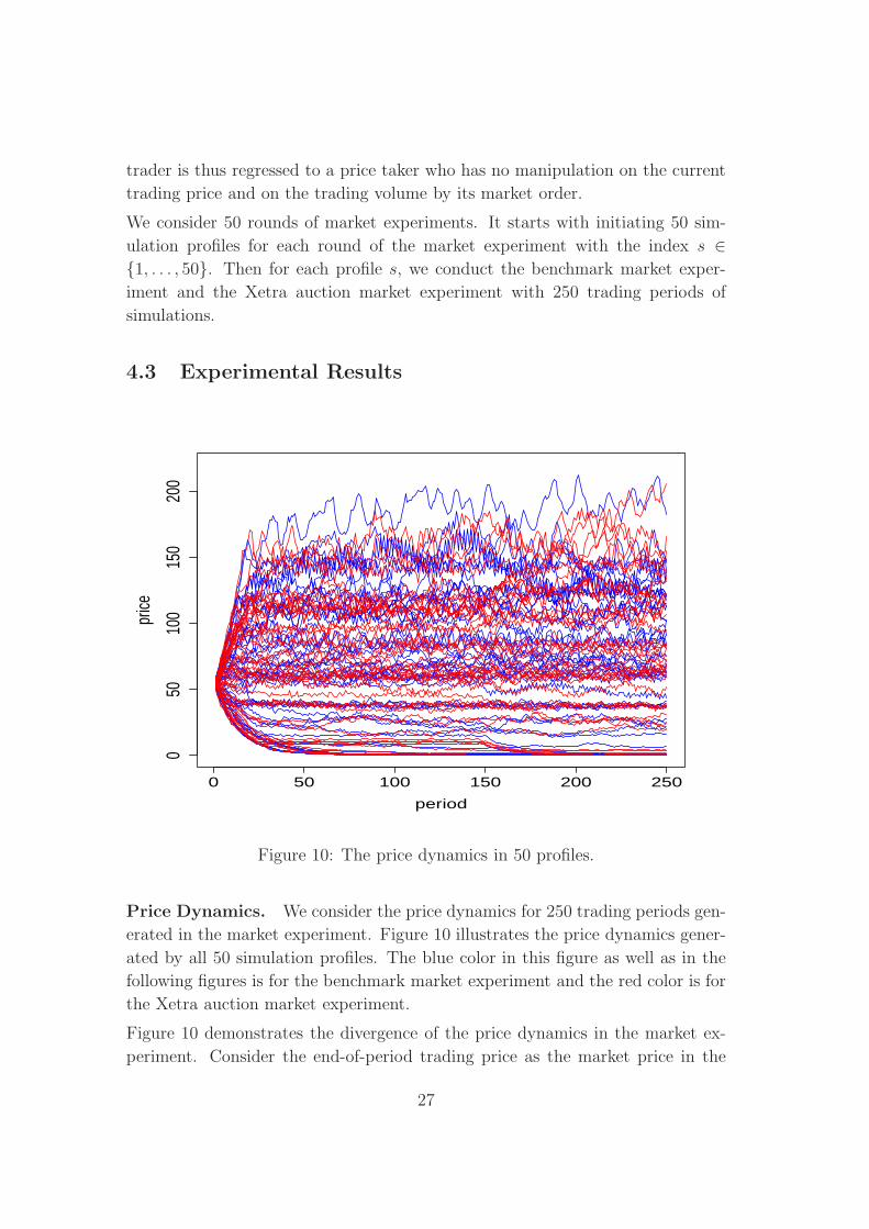
Figure 11: The histogram of the end-of-period trading price in the market exper-
iments.
last trading period t = 250. It ranges [0, 182.67] for all 50 benchmark market
experiments and [0, 205.39] for all 50 Xetra auction market experiments in the
simulation. The histogram of the end-of-period trading price depicted in Figure
11 illustrates the divergence emerges in both market experiments.
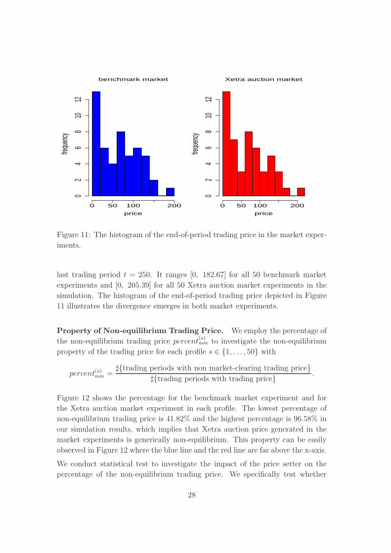
Property of Non-equilibrium Trading Price. We employ the percentage of
the non-equilibrium trading price percent(s)non to investigate the non-equilibrium
property of the trading price for each profile s ∈ {1, . . . , 50} with
percent(s)non =♯{trading periods with non market-clearing trading price}
♯{trading periods with trading price}.
Figure 12 shows the percentage for the benchmark market experiment and for
the Xetra auction market experiment in each profile. The lowest percentage of
non-equilibrium trading price is 41.82% and the highest percentage is 96.58% in
our simulation results, which implies that Xetra auction price generated in the
market experiments is generically non-equilibrium. This property can be easily
observed in Figure 12 where the blue line and the red line are far above the x-axis.
We conduct statistical test to investigate the impact of the price setter on the
percentage of the non-equilibrium trading price. We specifically test whether
28
Page 30
0 10 20 30 40 50
020
4060
8010
0
profile
perce
nt (%
)
Figure 12: The percentage of non market-clearing price.
percent(s)non associated with the benchmark market experiment is greater than that
associated with the Xetra auction market experiment. We apply the nonpara-
metric statistical test – the Wilcoxon signed ranks test – and verbally present
the null hypothesis as: percent(s)non in the benchmark market experiment is no
greater than that in the Xetra auction market experiment. The test result has
p− value = 0.0659 < 0.1. Thus, we reject the null hypothesis with 90% level
of confidence and accept that percent(s)non in the benchmark market experiment
is greater than that in the Xetra auction market experiment. Thus, the Xe-
tra auction market experiment where the price setter participates has a higher
percentage of market equilibrium than the benchmark market experiment. This
implies that the introduction of the price setter increases the possibility of market
equilibrium and thus increases the market efficiency in Xetra auction market.
Intuitively, when Xetra auction market exists a surplus, i.e., the discrepancy
between the aggregate demand and the aggregate supply, the price setter could
submit a market order to accept the surplus without affecting the trading price
in the market. When the price setter would submit a market order exceeding the
surplus, the trading price would jump to an inferior position such that the trading
price would fall down when the price setter would submit a market order in the
sell side and vice versa. Thus the price setter has the incentive to meet but not
outnumber the surplus in the market. When the price setter submits its market
29
Page 31
order to fully accept the surplus, Xetra auction market drives to equilibrium.
The introduction of the price setter thus increases the market efficiency in Xetra
auction market.
Price Volatility. We apply in this work the variance of the price dynamics
{P(s)X [1], . . . , P
(s)X [250]} for each profile s to measure price volatility in the market
experiment. The variance of the price dynamics is formulated as:
V ar(s) =1
249
250∑
n=1
(P(s)X [n]− P
(s)X )2,
where P(s)X is the mean value of {P
(s)X [1], . . . , P
(s)X [250]}. Figure 13 shows the
variance for the benchmark market experiment and for the Xetra auction market
experiment.
0 10 20 30 40 50
010
020
030
040
050
060
070
0
profile
varia
nce
Figure 13: The variance of the trading price dynamics.
We use the Wilcoxon signed ranks test to investigate the impact of the price setter
on the price volatility. The null hypothesis that we test is verbally presented as:
the variance on the price dynamics for the benchmark market experiment has
the same measure as that for the Xetra auction market experiment. The test
result has p− value = 0.8545. We can not reject the null hypothesis to accept
30
Page 32
that the variance on the price dynamics for the benchmark market experiment
is significantly different from that for the Xetra auction market experiment. It
seems that the introduction of the price setter does not significantly impact the
price volatility in Xetra auction market.
Intuitively the price setter influences the price volatility of Xetra auction market
in two different directions. The price setter exploits the market for a profit by
its aggressive trading behavior, which would increase the price volatility in Xetra
auction market. On the other hand, the introduction of the price setter increases
the possibility of market equilibrium. The increase in market efficiency would
allow traders to efficiently adjust their trading behavior to stabilize the market
in equilibrium, which implies a decrease in the price volatility of the market.
These two opposite impacts offset against each other so that the participation
of the price setter would not significantly influence the price volatility in Xetra
auction market.
5 Concluding Remarks
We have developed in this work the integrative framework for ACE modeling as
general guidance for analyzing economic systems from ‘bottom-up’ and for seam-
lessly transferring economic systems into the corresponding agent-based models.
By applying this integrative framework, we have constructed the agent-based
model of XAMS with the formulation of XAMM and of the price setter. The
success of developing the agent-based model of XAMS by applying the inte-
grative framework demonstrates that the modeling procedure and the modeling
templates applied in this framework are sufficiently applicable for analyzing the
economic system and for developing the corresponding agent-based model in a
step-by-step manner.
We have implemented the agent-based model with the computer software sys-
tem and have conducted the computer simulation for market experiments. By
investigating simulation results on market dynamics, we have discovered that
the introduction of the price setter improves market efficiency while does not
significantly influence price volatility in Xetra auction market.
The investigation of simulation results on market dynamics has validated the
property of non-equilibrium trading price in Xetra auction market. This finding
reveals the flexibility of the agent-based model in depicting non-equilibrium mar-
ket dynamics. Another flexibility of the agent-based modeling demonstrated in
our work is on the aspect of modeling active economic agents. We have applied
31
Page 33
MAEA to model heterogeneous traders in Xetra auction market with the mean-
variance preference in the submodule of objectives. Essentially the submodule
of objectives in MAEA presents the mechanism of selection that the agent em-
ploys to choose its action plan. By applying MAEA, one can easily extend the
model of traders by replacing the mean-variance preference with new criteria of
selection that allow more flavor of non-optimizing and adaptive behavioral rules.
One possibility is to introduce psychological patterns of decision making in the
trader’s submodule of objectives, which is open for the future work.
References
Bertalanffy, L. v. (1993). General system theory. New York: Braziller,
revised edition, 11. print. ed.
Blaha, M. & Rumbaugh, J. (2004). Object-Oriented Modeling and Design
with UML. Prentice Hall, second edition ed.
Das, S. (2003). Intelligent market-making in artificial financial markets. Mas-
ter’s thesis, Massachusetts Institute of Technology.
Domowitz, I. . & Yegerman, H. (2005). The cost of algorithmic trading:
A first look at comparative performance. In: Algorithmic Trading: Precision,
Control, Execution (Brian R. Bruce, P. A. M., ed.).
Gruppe Deutsche Borse (2003). The market model stock trading for Xetra.
Frankfurt a. M.
LeBaron, B. (2006). Agent-based computational finance. In: Handbook of
Computational Economics, Vol. 2: Agent-Based Computational Economics.
(Tesfatsion, L. S. & Judd, K. L., eds.), Handbooks in Economics Series,
chap. 9. North-Holland.
Li, X. (2010). Microeconomic Foundation of Investment Decisions for Elec-
tronic Security Trading Systems. Ph.D. thesis, Bielefeld Graduate School of
Economics and Management, Bielefeld University.
Merton, R. C. (1992). Continuous-Time Finance. Blackwell.
NYSE Euronext (2010). Euronext Rule Book - Book I.
Pindyck, R. & Rubinfeld, D. (2001). Microeconomics. Prentice Hall, 5th
edition ed.
32
Page 34
Potts, J. (2000). The new evolutionary microeconomics. New horizons in
institutional and evolutionary economics. Elgar.
Russell, S. J. & Norvig, P. (2003). Artificial intelligence, a Modern Ap-
proach. Prentice Hall series in artificial intelligence. Prentice Hall, 2. ed. ed.
Sharpe, W. (1964). Capital asset prices: A theory of market equilibrium under
conditions of risk. Journal of Finance 19(3), 425–442.
Tesfatsion, L. S. (2006). Agent-based computational economics: A contructive
approach to economic theory. In: Handbook of Computational Economics,
Vol. 2: Agent-Based Computational Economics (Tesfatsion, L. S. & Judd,
K. L., eds.). North-Holland.
33
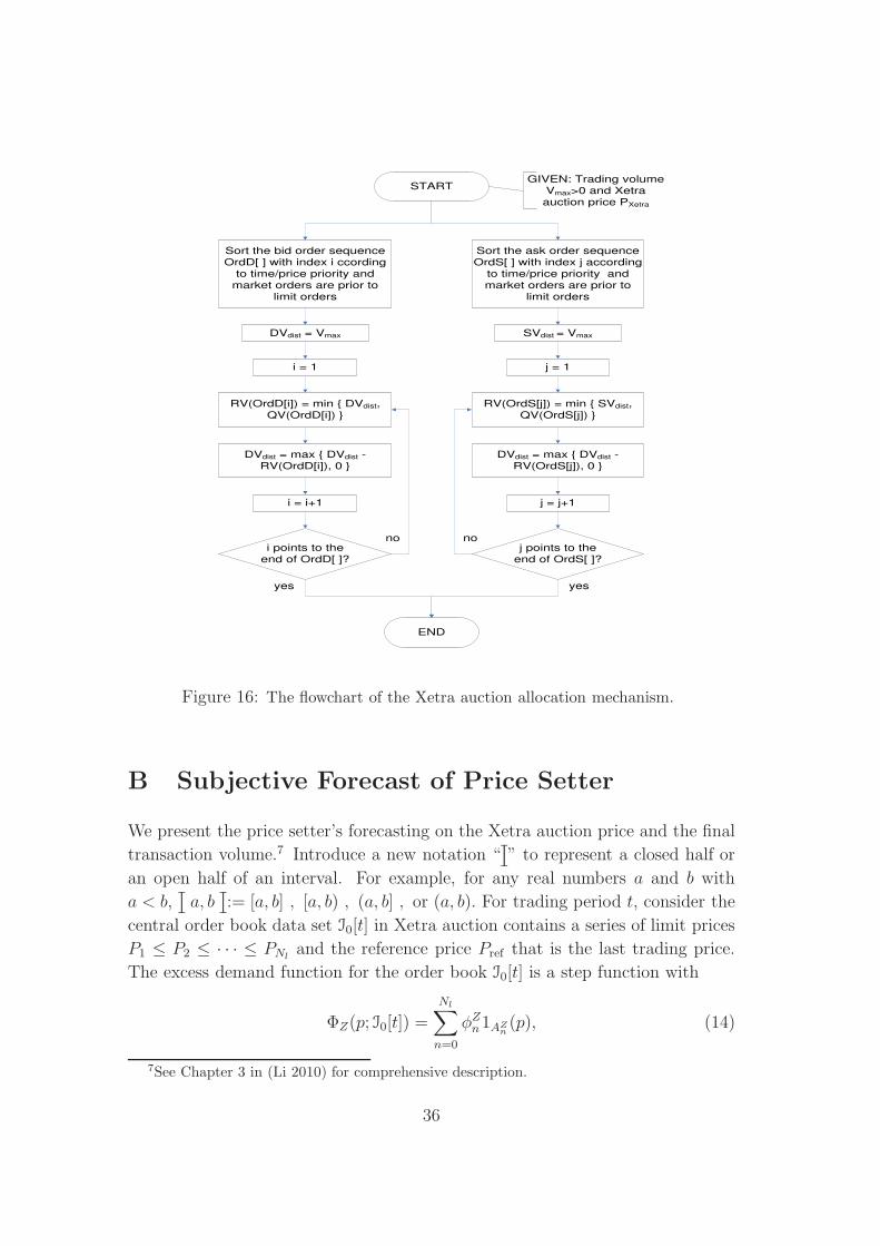
Page 35
A Xetra Auction Market Mechanism
The Xetra auction market mechanism is composed of the Xetra auction price
mechanism and the allocation mechanism to determine the Xetra auction price
and the trading volume respectively. Based on the description of the Xetra auc-
tion trading rules in (Gruppe Deutsche Borse 2003), Figure 14 illustrates the
Xetra auction price mechanism in which the subprocess Xetra-Auction-PDA(I0)
is depicted in Figure 15. The formulation of the Xetra auction allocation mech-
anism is illustrated in Figure 16.
START
GIVEN: order
book data set 0
Limit order exists?
( 0=ø? )
Market orders
in both sides of the
market?
RETURN: Pxetra = Pref
END
Vmax=0?
RETURN: no PXetra
SUBPROCESS:
Xetra-Auction-PDA( 0)
no
yes
yesyes
no
no
COMPUTE: Highest
trading volume Vmax for
all limit price p in 0
COMPUTE: the set of all
volume maximizing prices
V={p 0 | V(p) =Vmax}
RETURN: no PXetra
Figure 14: The flowchart of the Xetra auction price mechanism.
34
Page 36
Surplus on the demand side?
Z ZP 0?
END
COMPUTE: the lowest
surplus Zmin in V
Zmin={ | Z(p)| | p V }
START
COMPUTE: the lowest
candidate price with surplus on
the supply side
Pmax=min{p Z | Z(p)= � Zmin}
COMPUTE: the highest
candidate price with surplus on
the demand side
Pmin=max{p Z | Z(p) = Zmin}
RETURN:
PXetra=max{Pmin, min {Pref, Pmax}}
yes
no
yes
no
yes
no
yes
no
No Surplus?
Z Z Z ZP P 0?
Surplus on the supply side?
Z ZP 0?
RETURN: XetraP
Z ref Zmax P ,min P ,P
RETURN: Xetra ZP P
RETURN: Xetra ZP P
COMPUTE: The highest candidate price
ZP max Z
COMPUTE: The lowest candidate price
ZP min Z
Only one
candidate price?
# Z=1?
RETURN: XetraP ZP
for ZP Z
COMPUTE: the set of all
candidate prices with the
highest trading volume and
the lowest surplus
Z={p V | | Z(p)| =Zmin}
Figure 15: The flowchart of subprocess: Xetra-Auction-PDA(I0).
The function QV (Ord) in Figure 16 returns the quoted trading quantity of the
order Ord and the function RV (Ord) denotes the realized trading volume for the
order Ord.
35
Page 37
STARTGIVEN: Trading volume
Vmax>0 and Xetra auction price PXetra
END
RV(OrdD[i]) = min { DVdist,QV(OrdD[i]) }
DVdist = Vmax
DVdist = max { DVdist -RV(OrdD[i]), 0 }
i = 1
i = i+1
i points to the end of OrdD[ ]?
Sort the bid order sequence OrdD[ ] with index i ccording
to time/price priority and market orders are prior to
limit orders
Sort the ask order sequence OrdS[ ] with index j according
to time/price priority and market orders are prior to
limit orders
RV(OrdS[j]) = min { SVdist,QV(OrdS[j]) }
SVdist = Vmax
DVdist = max { DVdist -RV(OrdS[j]), 0 }
j = 1
j = j+1
j points to the end of OrdS[ ]?
yesyes
no no
Figure 16: The flowchart of the Xetra auction allocation mechanism.
B Subjective Forecast of Price Setter
We present the price setter’s forecasting on the Xetra auction price and the final
transaction volume.7 Introduce a new notation “[]
” to represent a closed half or
an open half of an interval. For example, for any real numbers a and b with
a < b,[]
a, b[]
:= [a, b] , [a, b) , (a, b] , or (a, b). For trading period t, consider the
central order book data set I0[t] in Xetra auction contains a series of limit prices
P1 ≤ P2 ≤ · · · ≤ PNland the reference price Pref that is the last trading price.
The excess demand function for the order book I0[t] is a step function with
ΦZ(p; I0[t]) =
Nl∑
n=0
φZn1AZ
n(p), (14)
7See Chapter 3 in (Li 2010) for comprehensive description.
36
Page 38
where φZn is a constant for n = 0, . . . , Nl and {AZ
0 , AZ1 , . . . , A
ZNl} is a partition of
R+ with AZ0 := [0, P1
[]
; AZn :=
[]
Pn, Pn+1
[]
for n = 1, . . . , Nl − 1; and AZNl
:=[]
PNl,+∞).
The price setter is to submit the market order Q(1)m [t] with Q
(1)m [t] > 0 denoting
a market order on the demand side and Q(1)m [t] < 0 denoting that on the supply
side. After the price setter submit its market order, the excess demand function
updates to the form
Φ′
Z(Q(1)m [t], p; I0[t]) = ΦZ(p; I0[t]) +Q(1)
m [t]
=
Nl∑
n=0
φZn1AZ
n(p) +Q(1)
m [t]. (15)
The price setter expects to be the last trader submitting order to the market.
Then the price setter’s forecast P eX(Q
(1)m [t]) on the upcoming Xetra auction price
is the step function:
P eX(Q
(1)m [t]) =
P1 when Q(1)m [t] ∈ (−∞,−φZ
1 );
P ∗
n when Q(1)m [t] = −φZ
n , n ∈ {1, 2, . . . , Nl − 1};
Pn when Q(1)m [t] ∈ (−φZ
n−1,−φZn ), n ∈ {2, 3, . . . , Nl − 1};
PNlwhen Q
(1)m [t] ∈ (−φZ
Nl−1,+∞);
(16)
where for any n ∈ {1, 2, · · · , Nl − 1}
P ∗
n =
Pn CASE 1;
Pn+1 CASE 2;
max{Pn,min{Pref , Pn+1}} CASE 3;
for CASE 1: either AZn = [Pn, Pn+1) or A
Zn = (Pn, Pn+1) with
|Φ′
Z(−φZn , Pn; I0[t]) |<|Φ
′
Z(−φZn , Pn+1; I0[t]) |;
for CASE 2: either AZn = (Pn, Pn+1] or A
Zn = (Pn, Pn+1) with
|Φ′
Z(−φZn , Pn; I0[t]) |>|Φ
′
Z(−φZn , Pn+1; I0[t]) |;
for CASE 3: either AZn = [Pn, Pn+1] or A
Zn = (Pn, Pn+1) with
|Φ′
Z(−φZn , Pn; I0[t]) |=|Φ
′
Z(−φZn , Pn+1; I0[t]) | .
Consider the notation a+ := max{0, a} and a− := min{0, a} for any a ∈ R. The
price setter’s forecast ZeX(Q
(1)m [t]) on the its final transaction volume is as:
ZeX(Q
(1)m [t]) = max{(−φZ
0 )−,min{Q(1)
m [t], (−φZI+J)
+}}. (17)
37