AUT Jouranl of Modeling and Simulation

AUT J. Model. Simul., 53(1) (2021) 1-10DOI: 10.22060/miscj.2021.19033.5229

Design and Modeling of an In-pipe Inspection Robot with Repairing Capability Equipped with a ManipulatorHami Tourajizadeh*, Samira Afshari, Meisam Azimi

Mechanical engineering Department, Faculty of Engineering, Kharazmi University, Tehran, Iran.

ABSTRACT: In this paper, an in-pipe inspection robot is designed and modeled with a manipulator to provide the manipulation ability. However, most of such robots are limited to perform inspecting operations. In order to design an in-pipe inspection robot capable of performing an operational task within the pipes, the robot is redesigned by adding a two-linkage serial manipulator with two extra DOFs on the main body of the moving robot. In this way, the robot will be a system with three degrees of freedom. The robot’s kinematic and dynamic models are obtained using Denavit-Hartenberg convention and Euler-Lagrange relations, respectively. Also, the system is controlled using inverse dynamics. Formulas verification, as well as analysis of its results, has been done by MATLAB software. The correctness of the model and the efficiency of the proposed manipulation are investigated by comparing the actual and desired paths. The proposed mechanism is efficient regarding ease and cost reduction. It will be seen that the mechanism is fully applicable for this robot to cover the operational tasks.

Review History:

Received: 2020-09-19Revised: 2021-04-26Accepted: 2021-04-30Available Online: 2021-06-15

Keywords:

In-Pipe Inspection Robot

Repairing Robot

Kinematic and Dynamic Modelling

Manipulator

1

*Corresponding author’s email: Tourajizadeh@khu.ac.ir

Copyrights for this article are retained by the author(s) with publishing rights granted to Amirkabir University Press. The content of this article is subject to the terms and conditions of the Creative Commons Attribution 4.0 International (CC-BY-NC 4.0) License. For more information, please visit https://www.creativecommons.org/licenses/by-nc/4.0/legalcode.

1. INTRODUCTIONAll over the world, pipelines widely exist in various

industrial structures, which require thorough inspections about every seven years. Since there are different conditions for the pipelines such as their environmental conditions, the fluid type which flows inside the pipeline, the pipe diameter, and so on, there is not always the possibility for the human entrance to do inspections. Applying robots here can be useful to reduce danger to humans and have more accurate performance. Therefore, in-pipe inspection robots are highly noticed in recent years, and different types of them have been introduced to deal with various challenges in these systems.

An important point in applying in-pipe robots is that they are supposed to perform manipulating operations in addition to inspections. Therefore, to fulfill the expectations, different structures have been introduced with appropriate control methods. The most renowned types of in-pipe robots are the caterpillar type, the wheeled type, the legged type, the inchworm type, the snake type, the screw type, and the PIG type. Among the mentioned categories, wheeled type in-pipe robots are the most applicable systems since they can provide the highest maneuverability. A wheeled type in-pipe robot has a high level of stability since the pipe wall in these robots tolerates an additional force except the robot’s weight, which significantly affects the stability of such robots during the manipulation operation. Moreover, the wheeled type in-pipe robots are categorized in two ways. In the first

one, these robots are Caterpillar wall-pressed type or wheeled wall-pressed type. Also, the second classification includes the simple type and the screw one[1].

In the research history of in-pipe robots, it can be observed that Fukuda et al. proposed an inchworm-type in-pipe inspection robot[2], while Roman and Pellegrino introduced a caterpillar type of this robot[3]. Due to the better stability of wall-pressed robots, Iwashina et al. proposed a wall-pressed in-pipe inspection robot that is capable of moving through sloped pipelines[4]. The kinematic modeling of this type was noticed by Kwon and Yi, who introduced the kinematic model of an in-pipe inspection robot with three caterpillar wheel chains[5]. Also, Zhang and Yan developed an in-pipe robot that is adaptable to different sizes of pipe diameter and automatically adjusts the tractive force. The proposed robot in this study can be applied in the long distances of pipelines with different diameter series[6].

Control of in-pipe inspection robots is the problem in which the research history is still poor. Kwon et al. studied the motion planning of a two-module indoor pipeline inspection robot [7]. Zhang and Chen applied the fuzzy algorithm to control a mobile pipeline robot [8]. Also, Gregory et al. used the optimal control method to plan the optimal path of a system with holonomic constraints[9]. Despite the extensive research that has been done on in-pipe inspection robot systems, a lack of research work on proposing a proper mechanism of end-effector and its appropriate controller to do repairs is perceived. As mentioned, the introduced

UNCORRECTED PROOF

H. Tourajizadeh et al., AUT J. Model. Simul., 53(1) (2020) 1-10, DOI: 10.22060/miscj.2021.19033.5229

2

systems are only capable of inspecting pipelines and are not able to do operations such as repairing. Therefore, in this paper, the proper mechanism of a wall-pressed in-pipe robot is proposed, which is equipped with a manipulator to make it capable of doing the required operations. The kinematic model in the proposed robot system is extracted by the Denavit-Hartenburg method. Moreover, its dynamic model and the related motion equations are derived using the Euler-Lagrange formulation[10]. In order to verify the extracted kinematic and dynamic models, the simulations are considered in both forward and inverse approaches. By determining the values of required parameters and analysis by MATLAB, the simulation results are presented.

The current study consists of 5 main sections. Modeling of the system is extracted in the next section. Here, both the kinematic and dynamic models of the system are extracted. In the third section, an appropriate control method is employed to provide the required robustness of the system for tracking purpose. In the Simulation section, first, some MATLAB simulations are conducted to verify the extracted models. Then, the efficiency of the proposed controller is studied in a similar way. Finally, in the conclusion section, the analytical results and the comprehensive explanation regarding the extracted model of the system are delivered. It is shown that by the aid of the proposed robot and the designed controller, the mentioned inspectional and operational tasks are possible to be performed successfully within a pipeline.

2. MODELINGFigure 1 shows a schematic view of the robot and its

position in a pipeline. In this section, both the kinematic and kinetic models are introduced based on the following assumptions:

Assumption 1: In the proposed mechanism, the length of each wheeled link can be adjusted according to the pipeline diameter. Therefore, the proposed inspection robot can be applicable in pipes with different diameters. However, the related diameter should be constant all over the pipeline.

Assumption 2: As shown in Fig. 1, the angle between every two legs is 120° , and the legs are entirely along the pipe axis. Therefore, the robot does not rotate about the mentioned axis.

Assumption 3: The pipeline is considered to be a straight line, and so, the wheels rotate equally.

Assumption 4: In order to calculate the potential energy of the system, the pipe axle is assumed to be the reference level.

Assumption 5: It is supposed that the static friction is enough to prevent slippage.

Assumption 6: The pipeline is supposed to be empty, and thus, no drag force is involved.

2-1-KinematicsIn this section, the kinematic model of the robot is

extracted, considering forward and inverse approaches. In the forward approach, the end-effector position in its workspace can be calculated according to the joint space variables. Also, through the inverse approach of the kinematic model, the position of each joint space variable can be calculated according to the workspace variables.

Considering the forward approach in the kinematic model, it is supposed to calculate the workspace path according to the joint space variables. To do so, the Denavit-Hartenburg method is applied as follows [10]. By using the D-H method, the translation in every link includes four consecutive transfers, two of which are translational, and the two others are rotational. The mentioned transfer matrix between every two links is defined as:

0 0 10 0 0 1

i i i i i i

i i i i i i

i

ii

i

C S C S S a C

S C C C S a SA

d

θ θ α θ α θ

θ θ α θ α θ

− =

(1)

Here, C and S are the cosine and sine symbols, respectively. a and d are the linear transfers of the coordinate in meters, θ and α are the rotational transfers in radians and the index i refers to the link number. As mentioned, the robot system should be equalized to some links. Considering 1β to be the initial rotation angle about the pipe axle ( 0z axis), in radians, and also considering that the robot moves along the pip-line as the linear transfer along the 0z axis, the distance between the robot and the global coordinate system is the first link whose length is equal to rθ , in meters, and is rotated by 1β . In fact, 1β is the angle, in radians, by which the robot takes place inside the pipeline. D-H parameters are mentioned in Table

Fig. 1 The schematic view of the proposed robot

   

Fig. 1. The schematic view of the proposed robot

UNCORRECTED PROOF

3

H. Tourajizadeh et al., AUT J. Model. Simul., 53(1) (2020) 1-10, DOI: 10.22060/miscj.2021.19033.5229

1. The robot’s first link is considered to be the second link in the D-H transfer, and the robot’s second link is considered to be the third link in it, similarly. The end-effector position according to the third local coordinate system is denoted by 3p . Figure 2 shows a schematic view of equalizing the proposed robot with serial robots by which the information required in the D-H table can be derived.

[ ]3 0 0 0 1 Tp =

(2)

In Eq. (2), 3p denotes the position of the end-effector according to the third local coordinate system, as mentioned. Using the parameters shown in Fig. 2, the D-H table can be formed to extract the kinematic model. The values of mentioned parameters are gathered in table 1.

Therefore, we have:

1 2

1 2

0 0

2

23 1 2 3 3 3 3

1

1 1

a Cxy a S

p A A A p A pz r a

β β

β β

θ

+

+

= = = = +

(3-a)

where 1a and 2a are the length of the first and second link, in meters, relatively. 1β is the robot’s initial rotate angle about 0z axis, 2β is the rotate angle of the first and second link about 0z axis, both in radians, r is the radius of each wheel, in meters, and θ denotes the rotation angle of each wheel, in radians. iA is the transfer matrix related to the link , and

3_ 0P denotes the position of the end-effector according to the global coordinate system. Therefore, the forward position kinematic model can be shown as equation (3-a) in which the joint space variables vector and the workspace variables one are introduced as follows:

2

2

qa

θβ =

(3-b)

xp y

z

=

(3-c)

In order to analyze the kinematic relations between velocity vectors in the joint space and the workspace, the Jacobian matrix should be calculated using Eq. (4).

1 2 1 2

1 2 1 2

2

2

0

0

0 0

a S CpJ a C Sq

r

β β β β

β β β β

+ +

+ +

− ∂

= = ∂

(4)

Finally, the workspace velocity vector can be calculated using Eq. (5):

1 2 1 2

1 2 1 2

2 2 2

2 2 2

a C a S

p Jq a S a C

r

β β β β

β β β β

β

β

θ

+ +

+ +

−

= = +

(5)

where p and q are the velocity vectors in the workspace and joint space of the robot, respectively. 2a is the rate of the second link’s length variation, in meters per second and θ is the angular velocity of the wheels, in radians per second. The rest of the parameters in Eq. (5) have already been introduced in the former explanations. In order to have the inverse kinematic model, the joint space variables vector should be calculated according to the workspace variables using equation (3-a). Thus, we have:

( )1

12 1

2 2 2

tan

z aryqx

ax y

θβ β−

− = = − +

(6)

Table 1 D-H parameters

Link number 𝑎𝑎� 𝛼𝛼� 𝑑𝑑� 𝜃𝜃� 1 0 0 𝑟𝑟𝜃𝜃∗ 𝛽𝛽�

2 0 0 𝑎𝑎� 𝛽𝛽�∗ 3 𝑎𝑎�∗ 0 0 0

Table 1. D-H parameters

Fig. 2 D-H coordinate systems

 

   

   

Fig. 2. D-H coordinate systemsUNCORRECTED PROOF

H. Tourajizadeh et al., AUT J. Model. Simul., 53(1) (2020) 1-10, DOI: 10.22060/miscj.2021.19033.5229

4

where x , y , and z , in meters, are the three components of the end-effector position vector, according to the global coordinate system. Other parameters in Eq. (6) have already been explained.

Using the Jacobian matrix, the inverse model of the velocity can be written as follows:

1q J p−= (7)

where q and p are the joint space and the workspace velocity vectors, relatively. Also, J is the Jacobian matrix of the system, which is calculated in Eq. (4).

2-2-DynamicsExtracting motion equations of the system is one of the

most important parts of this paper. Using motion equations, the robot’s motion can be understood well. Additionally, these equations are used to design an appropriate controller for the system. Analysis of the dynamic model is considered here in both the forward and inverse approaches, similar to the kinematic model. In the inverse approach, the required amounts of forces and torques are calculated by which a specific path in each joint space variable can be tracked. Moreover, through the forward approach, joint space paths are calculated considering the implementation of specific values as the input torques and forces. Therefore, the two mentioned approaches are discussed separately.

In order to conduct a dynamic analysis of the system through the inverse approach and calculate motion equations by the Lagrange method, firstly, it is required to calculate the Lagrangian of the system using the kinetic and the potential energies [10]. The total kinetic energy of the system is calculated in Eq. (8):

( )

2 2 2total 1 2 3 4 5 6 2 2 2 2

2 2 2 2 2 21 1 2 1 2

1 16 2

1 1 334 2 4b w w

K K K K K K K a m a

m r r m m m m m r

β

β θ θ

= + + + + + = + +

+ + + + +

(8)

where totalK is the total kinetic energy of the system, 1K is the translational kinetic energy of the robot body, 2K is the kinetic energy related to the wheels’ rotation, 3K is the kinetic energy resultant of the prismatic motion in the second link,

4K is the kinetic energy related to the translational motion of the center of mass in the second link resultant of its rotation about the first link axle, 5K is the rotational kinetic energy of the second link and 6K is the first link’s rotational kinetic energy. All the mentioned energy amounts are calculated in Joules. Moreover, wm is the wheel’s mass, bm is the mass of the robot body, 1m is the first link’s mass, and 2m is the second one’s, all in kilograms. 1r is the radius of the first link’s cross-section, in meters, and finally, 2β is the angular velocity of the first and second link about the 0z axis, in radians per second.

As mentioned before, the pipe axle is assumed to be the reference level to calculate the potential energy of the system. Thus, the only part of the robot which has a noticeable amount

of potential energy is its second link. The y component in the global coordinate system is related to the second link’s center of mass. Therefore, by multiplying the transfer matrix in the center of mass coordinate, the mentioned component can be calculated according to the global coordinate system.

2 2 0 2

0.5 0 0 00 1 0 00 0 1 00 0 0 1

aCm A p−

=

(9)

Here, 2aCm is the second link’s center of mass coordinate

according to the global coordinate system. Also, 2 0A − is the transfer matrix between the local coordinate systems of 2 and 0, and 2p is the end-effector position according to the 2nd local coordinate system. By Simplifying Eq. (2) and considering the component related to the height, we have:

2 1 220.5 ah a Sβ β+=

(10)

where, 2ah denotes the height of the second link’s center

of mass, in meters, according to the reference potential level. Therefore, the total potential energy of the system is as follows:

2 2 2 1 2total 20.5 a a aP m gh m ga Sβ β+= = (11)

where g is the gravitational acceleration. The Lagrangian of the system is as Eq. (12):

( )2 1 1

1 2 2 1 2

2 2 2 2 2total total 2 2 2 2

2 2 2 22

1 1 16 2 4

1 3 132 4 2

a a a

a a b w w a

La K P a m a m r

r m m m m m r m ga Sβ β

β β

θ θ +

= − = + + +

+ + + + −

(12)

Therefore, the motion equations of the system can be extracted as follows:

ii i

d La Ladt q q

τ ∂ ∂

= − ∂ ∂

(13)

Finally, dynamic equations of the robot can be written as Eq. (14):

2

2

1

2

3 af

θ

β

τ ττ τ τ

τ

= =

(14)

( )1 2

¨21 2 2 2 9

2 a a b wr m m m mθτ θ= + + +

2 2 1 1 2 1 2

¨2 2

2 2 21 1 13 2 2a a a am a m r m ga Cβ β βτ β +

= + +

2 2 1 2

¨2

22 21 2 6 36a af m a a gSβ ββ +

= − + +

UNCORRECTED PROOF

5

H. Tourajizadeh et al., AUT J. Model. Simul., 53(1) (2020) 1-10, DOI: 10.22060/miscj.2021.19033.5229

Here, θτ is the total torque amount of three wheels, and

2βτ is the required torque of the first link, both in Newton-meters. Also,

2af is the prismatic force of the second link, in Newtons. Since the inverse dynamic model of the system is now available, the required input values can be extracted according to the desired paths for joint space variables.

To extract the forward dynamic model as well, the motion equations should be rewritten in the following form:

( ) ( )¨

,M q q CG q qτ = +

(15)

where q , q and ¨q are the position, velocity, and

acceleration of the joint space vector, respectively, according to the global coordinate system. Also, the matrices that are mentioned in this equation are as follows:

( )1

2

3

0 00 00 0

MM q M

M

=

; (16)

( )1 2

21

1 2 2 2 92 a a b wM r m m m m= + + +

2 1 1

2 22 2

1 13 2a a aM m a m r= +

23 aM m=

( )2 1 2

2 1 2

2

22 2

01,2

1 12 3

a

a

CG q q m ga C

m gS a

β β

β β β

+

+

= −

(17)

Here, ( )M q is the inertia matrix, and ( ),CG q q includes the Coriolis terms and gravitation. As it is shown, ( ),CG q qis a function of both the position and derivation of the joint variables. Therefore, the joint space acceleration vector can be written according to the rest of the parameters:

( )

¨

¨ ¨1

2¨

2

q M CG

a

θ

β τ−

= = −

(18)

As explained before, the forward dynamic model is the system response to the implementation of specific values of input torques and forces. Thus, it is necessary to calculate the acceleration vector of joint space variables according to the determined vector pf torques and forces. Afterward, the

position vector of joint space variables can be derived by solving the resultant differential equations. Thus, we have:

[ ]1 2 3Tτ τ τ τ=

(19)

11

1 12

13

0 00 00 0

MM M

M

−

− −

−

=

; (20)

( )1 2

11 2

22 2 2 9a a b w

Mr m m m m

− =+ + +

2 1 1

12 2 2

2

62 3a a a

Mm a m r

− =+

2

13

1

a

Mm

− =

( )

( )

1 2

2 1 2

2 1 1

2 1 2

2

12

2 2¨

2 22

23 2 2

22 2 2 9

162

2 3

1 2 36

a a b w

a

a a a

a

a

r m m m m

m ga Cq

m a m r

m a gS

m

β β

β β

τ

τ

τ β

+

+

+ + + −

= +

− − +

(21)

Eq. (21) shows the joint space acceleration resultant of a specific vector of input torques and forces. Solving this equation results in getting the joint space vector path, which has been done in MATLAB, and the results are presented in the following sections.

3. CONTROLIn this section, a proper controller is designed to control

the position of the robot and the accuracy of its performance, considering that the kinematic and dynamic models have already been extracted. An open-loop control method is noticed here using the inverse dynamic model. The total amount of input vector which should be applied to the robot system consists of the following types:

First, the required inverse dynamic input by which the joint space variables track the desired trajectory in the absence of external force. This type of input is denoted by dynτ and is calculated in Eq. (22). The second one is resτ in Eq. (22), which is the resultant torque and force on the joints due to the presence of external force during the repairment operations. The third type of input vector is the controller reaction to the position error of the end-effector. Its value is calculated according to the error between the actual and desired paths of joint variables. In other words, calculating contτ in Eq. (22), requires the error and its rate to be measured during the simulation time. In ideal circumstances, the error value and its rate are both equal to zero, and consequently, contτ also

UNCORRECTED PROOF

H. Tourajizadeh et al., AUT J. Model. Simul., 53(1) (2020) 1-10, DOI: 10.22060/miscj.2021.19033.5229

6

equals 0. Summation of the three mentioned type of inputs is considered the total amount of control input and is shown as

totτ in Eq. (22).

tot dyn res contτ τ τ τ= + +

(22)

Where:

res 2 2

2 2

; d d

fyJF F f

y zzf

y z

τ µ

µ

= − = +

+

(23)

In Eq. (23), µ is the coefficient of friction between the inner surface of the pipeline and the robot wheels. f is the normal force, in Newtons, implemented on the robot from the pipe surface. It is among parameters determined in Table 2, and can be set according to the required frictional force. The less is the coefficient of friction, the more normal force value should be implemented on the inner surface of the pipe, which can be adjusted by setting thelength of the robot leg. Therefore, the value of f is assumed with respect to the friction force, and then, it is projected on the other two axes on the tangent surface of the pipe. Assuming the robot wheels to role without slippage, the formulation of rolling friction is applicable here, which is shown in Eq. (23). Also, ( ), ,x y z is the velocity vector of the end-effector in its workspace, and in Newton-meters as well as the other values of torques. Moreover, contτ in Eq. (22) is:

cont Ke Leτ = +

(24)

where and L are the proportional and derivative coefficients of the controller, respectively. Also, e and e are respectively the position error and the velocity error of the

joint space vector, which are calculated by Eq. (25).

; d a d ae X X e X X= − = −

(25)

In Eq. (25), dX is the desired vector of joint space position, and aX is the actual one in meters. To show the robustness of the designed controller, a sample disturbance is applied to the system to check the performance of the robot. The considered disturbance is a harmonic function with 0.1 amplitude of the inverse dynamic torque and the frequency of an ordinary vibrational mechanical system. This function is applied to the joints of the system as a disturbing torque. Therefore, we have:

in tot (1 0.2sin80 )tτ τ= + (26)

where totτ is the total amount of force and torque vector calculated in Eq. (22), and inτ is the control input applied to the system. Figure 3 shows the overall view of the presented control method.

In this paper, the summation of two controlling signals is employed, consisting of impedance control accompanied by computed torque method. With the aid of the computed torque method, the desired path can be tracked while the robustness of the system in presence of disturbances can be compensated by the added PD controller. Using the impedance controller, the applied external forces on the end-effector can be neutralized. It is proved in [11] that these two controlling strategies are stable.

4. SIMULATIONAll the required parameters to run the simulations are

given in table 2, and the simulation results are presented in the relevant parts. Then, the results can be analyzed to reach a comprehensive conclusion.

Moreover, the matrix K (the proportional coefficient matrix) and L (the derivative coefficient matrix) are considered as follows:

1.5 0 00 0.5 00 0 0.5

K =

; 1 0 00 1 00 0 1

L =

Table 2 Simulation parameters

symbol value unit 𝑟𝑟 0.12 m 𝑟𝑟� 0.05 m 𝛽𝛽� 0 rad g 9.81 m/s�𝑚𝑚� 0.5 kg 𝑚𝑚� 0.1 kg 𝑚𝑚� 0.2 kg 𝑚𝑚� 0.2 kg 𝑎𝑎� 0.2 m 𝑓𝑓 2 N 𝜇𝜇 0.1 -

Table 2. Simulation parameters

UNCORRECTED PROOF

7

H. Tourajizadeh et al., AUT J. Model. Simul., 53(1) (2020) 1-10, DOI: 10.22060/miscj.2021.19033.5229

4-1-KinematicsAssuming the desired trajectory of Eq. (27) for workspace

variables, the according joint space paths can be derived by the inverse kinematic model presented in Eq. (7). Figure 4 shows the joint space paths according to the desired workspace paths of Eq. (27):

0.19cos4

0.19sin4

0.384

t

xty

zt

=

(27)

Considering the output of the inverse model to be the input of the forward model, the results can be compared to investigate the correctness of the kinematic model. As Fig. 5 shows, the input paths of the inverse kinematic model conform to output paths of the forward case, reasonably. Therefore, it can be concluded that the extracted kinematic model is correct.

4-2-DynamicsIn order to verify the extracted dynamic model, the same

procedure of kinematic verification is considered. First, the required input force and torque vector is calculated by the inverse dynamic model, according to a specific desired path of the joint space vector. Then, the calculated input vector is implemented on the system, and it is supposed to see the system response in accordance with the original desired path. In other words, the two inverse and forward dynamic models are coupled with each other, and the results are compared. Equation (28) presents the considered desired path of the joint space vector according to time (in seconds), which is supposed to be compared in the inverse and forward dynamic models.

2

2

0.120.30.19

tq t

a

θβ = =

(28)

Figure 6 shows the calculated input amounts, which are derived from the inverse dynamic model.

Applying the calculated input values of Fig. 6 to the forward dynamic model of the system, the actual paths of joint space variables are extracted. Figure 7 shows the comparison between the desired and actual paths of joint space variables.

Fig. 3 The proposed control method diagram

   

Fig. 3. The proposed control method diagram

Fig. 4 The inverse kinematic response according to the desired workspace path

   

Fig. 4. The inverse kinematic response according to the desired workspace path

UNCORRECTED PROOF

H. Tourajizadeh et al., AUT J. Model. Simul., 53(1) (2020) 1-10, DOI: 10.22060/miscj.2021.19033.5229

8

As expected, the conformance of joint space paths in the inverse and forward approaches shows the correctness of the extracted dynamic model.

4-3-ControlIn this section, the desired path for the joint space vector

is considered to be as Eq. (29) shows:

( )

2

2

15sin 0.1

5cos15

0.4

d

d d

d

ttq

a

θβ

= =

(29)

Moreover, the control input vector is calculated by Eq.

Fig. 5 Comparison of the workspace paths in the inverse and forward kinematic models

   

Fig. 6 The inverse dynamic response to the desired path of the joint space vector

   

Fig. 5. Comparison of the workspace paths in the inverse and forward kinematic models

Fig. 6. The inverse dynamic response to the desired path of the joint space vector

Fig. 7 Comparison between the joint space paths in the inverse and forward dynamic models

   

Fig. 7. Comparison between the joint space paths in the inverse and forward dynamic models

UNCORRECTED PROOF

9

H. Tourajizadeh et al., AUT J. Model. Simul., 53(1) (2020) 1-10, DOI: 10.22060/miscj.2021.19033.5229

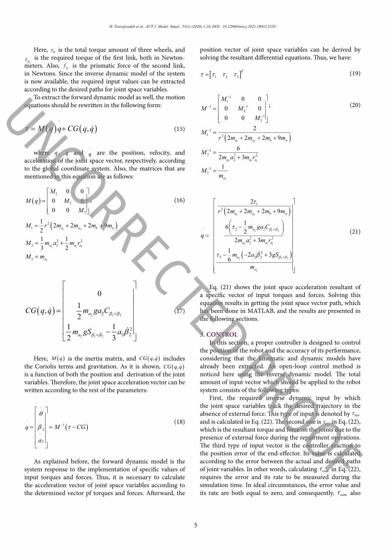
(26), as Fig. 8 shows:The mentioned control input is applied to the system, and

the actual response of the system is extracted. According to the presence of the mentioned harmonic disturbance, the oscillating torque is required to neutralize the disturbance. Thus, the robot will not fail in real scenarios, and its stability will be provided since the required torque to neutralize the applied harmonic disturbance is calculated and applied to the robot. Indeed, the summation of the torque of this figure together with the applied disturbance results in the required inverse dynamic torque of the robot to track the desired path.

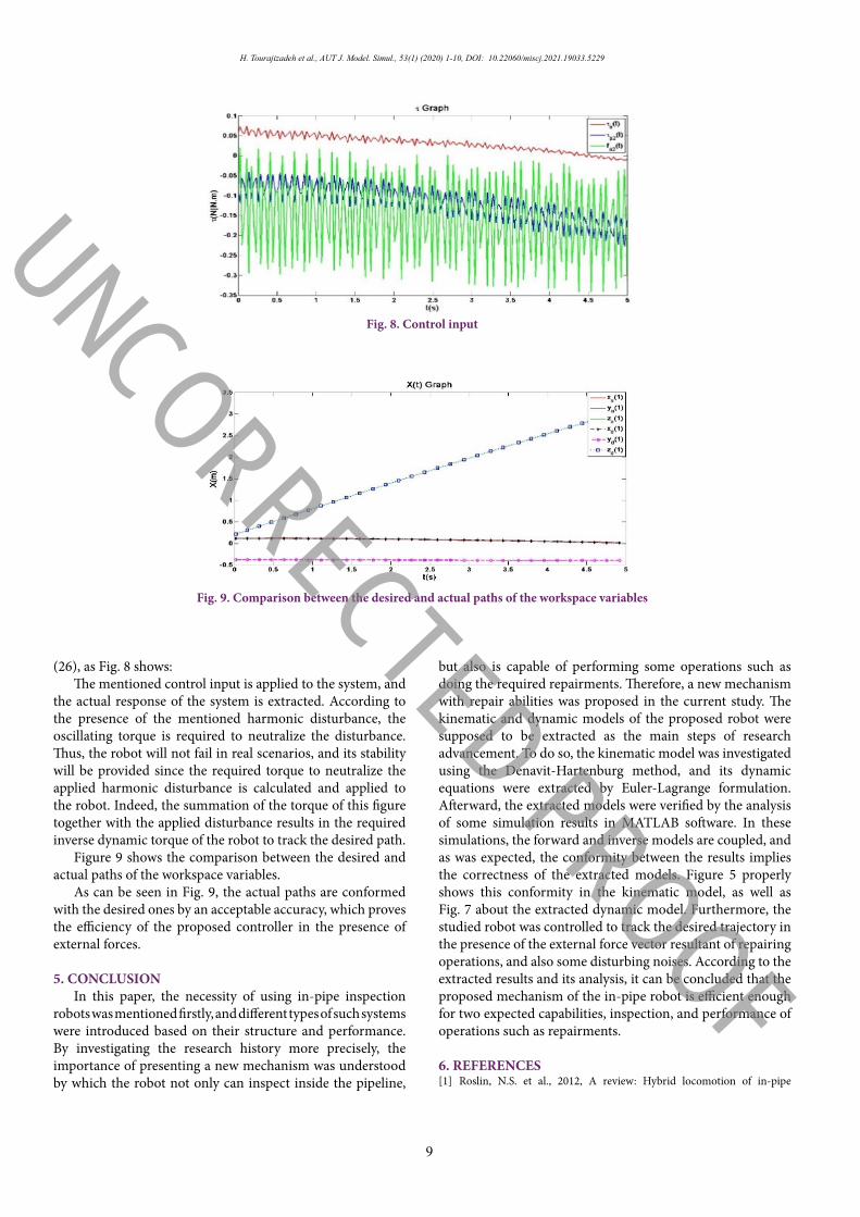
Figure 9 shows the comparison between the desired and actual paths of the workspace variables.

As can be seen in Fig. 9, the actual paths are conformed with the desired ones by an acceptable accuracy, which proves the efficiency of the proposed controller in the presence of external forces.

5. CONCLUSIONIn this paper, the necessity of using in-pipe inspection

robots was mentioned firstly, and different types of such systems were introduced based on their structure and performance. By investigating the research history more precisely, the importance of presenting a new mechanism was understood by which the robot not only can inspect inside the pipeline,

but also is capable of performing some operations such as doing the required repairments. Therefore, a new mechanism with repair abilities was proposed in the current study. The kinematic and dynamic models of the proposed robot were supposed to be extracted as the main steps of research advancement. To do so, the kinematic model was investigated using the Denavit-Hartenburg method, and its dynamic equations were extracted by Euler-Lagrange formulation. Afterward, the extracted models were verified by the analysis of some simulation results in MATLAB software. In these simulations, the forward and inverse models are coupled, and as was expected, the conformity between the results implies the correctness of the extracted models. Figure 5 properly shows this conformity in the kinematic model, as well as Fig. 7 about the extracted dynamic model. Furthermore, the studied robot was controlled to track the desired trajectory in the presence of the external force vector resultant of repairing operations, and also some disturbing noises. According to the extracted results and its analysis, it can be concluded that the proposed mechanism of the in-pipe robot is efficient enough for two expected capabilities, inspection, and performance of operations such as repairments.

6. REFERENCES[1] Roslin, N.S. et al., 2012, A review: Hybrid locomotion of in-pipe

Fig. 8 Control input

   

Fig. 9 Comparison between the desired and actual paths of the workspace variables

 

Fig. 8. Control input

Fig. 9. Comparison between the desired and actual paths of the workspace variables

UNCORRECTED PROOF

H. Tourajizadeh et al., AUT J. Model. Simul., 53(1) (2020) 1-10, DOI: 10.22060/miscj.2021.19033.5229

10

inspection robot, Procedia Engineering 41: p. 1456-1462.[2] Fukuda, T., Hosokai, H., and Uemura, M., 1989, Rubber gas actuator

driven by hydrogen storage alloy for in-pipe inspection mobile robot with flexible structure, in Robotics and Automation, Proceedings, IEEE International Conference on. 1989. IEEE.

[3] Roman, H.T., Pellegrino, B., and Sigrist, W., 1993, Pipe crawling inspection robots: an overview, IEEE transactions on energy conversion 8(3): p. 576-583.

[4] Iwashina, S., et al., 1994, Development of in-pipe operation micro robots, in Micro Machine and Human Science, Proceedings., 5th International Symposium on. 1994. IEEE.

[5] Kwon, Y.-S., Yi., B.-J, 2009, The kinematic modeling and optimal paramerization of an omni-directional pipeline robot, in Robotics and Automation, ICRA’09. IEEE International Conference on. 2009. IEEE.

[6] Zhang, Y., Yan, G., 2007, In-pipe inspection robot with active pipe-

diameter adaptability and automatic tractive force adjusting, Mechanism and Machine Theory 42(12): p. 1618-1631.

[7] Kwon, Y.-S. et al., 2008, Design and motion planning of a two-moduled indoor pipeline inspection robot. in Robotics and Automation, ICRA 2008, IEEE International Conference on. 2008. IEEE.

[8] Zhang, X., Chen, H., 2003, Independent wheel drive and fuzzy control of mobile pipeline robot with vision, in Industrial Electronics Society, IECON’03. The 29th Annual Conference of the IEEE. 2003. IEEE.

[9] Gregory, J., Olivares, A., and Staffetti, E., 2012, Energy-optimal trajectory planning for robot manipulators with holonomic constraints, Systems & Control Letters 61(2): p. 279-291.

[10] Spong, M.W., Hutchinson, S., and Vidyasagar, M., 2006, Robot modeling and control, Vol. 3. Wiley New York.

[11] Asada, H., Slotine, J.-J., 1986, Robot analysis and control, John Wiley & Sons.

HOW TO CITE THIS ARTICLEH. Tourajizadeh, S. Afshari, M. Azimi, Design and Modeling of an In-pipe Inspection Robot with Repairing Capability Equipped with a Manipulator, AUT J. Model. Simul., 53(1) (2021) 1-10.

DOI: 10.22060/miscj.2021.19033.5229

UNCORRECTED PROOF