Author's personal copy - UC Santa Barbara

This article appeared in a journal published by Elsevier. The attachedcopy is furnished to the author for internal non-commercial researchand education use, including for instruction at the authors institution

and sharing with colleagues.

Other uses, including reproduction and distribution, or selling orlicensing copies, or posting to personal, institutional or third party

websites are prohibited.

In most cases authors are permitted to post their version of thearticle (e.g. in Word or Tex form) to their personal website orinstitutional repository. Authors requiring further information

regarding Elsevier’s archiving and manuscript policies areencouraged to visit:

http://www.elsevier.com/copyright

http://www.elsevier.com/copyright

Author's personal copy

A stabilized explicit Lagrange multiplier based domaindecomposition method for parabolic problems q

Zheming Zheng a,*, Bernd Simeon b, Linda Petzold a

a Department of Mechanical Engineering, University of California Santa Barbara, Santa Barbara, CA 93106, USAb Zentrum Mathematik, Technische Universitat Munchen, Boltzmannstrasse 3, D-85748 Garching bei Munchen, Germany

Received 22 June 2007; received in revised form 23 January 2008; accepted 24 January 2008Available online 14 February 2008

Abstract

A fully explicit, stabilized domain decomposition method for solving moderately stiff parabolic partial differential equa-tions (PDEs) is presented. Writing the semi-discretized equations as a differential-algebraic equation (DAE) system wherethe interface continuity constraints between subdomains are enforced by Lagrange multipliers, the method uses the Run-ge–Kutta–Chebyshev projection scheme to integrate the DAE explicitly and to enforce the constraints by a projection.With mass lumping techniques and node-to-node matching grids, the method is fully explicit without solving any linearsystem. A stability analysis is presented to show the extended stability property of the method. The method is straightfor-ward to implement and to parallelize. Numerical results demonstrate that it has excellent performance.� 2008 Elsevier Inc. All rights reserved.

Keywords: Non-overlapping domain decomposition; Lagrange multiplier; Runge–Kutta–Chebyshev; Stability; Parallelization; ParabolicPDE

1. Introduction

Domain decomposition methods (DDM) for the solution of partial differential equations (PDEs) haveattracted a great deal of research interest, due to their flexibility for both multiphysics and parallel computing.For complex multiphysics problems, domain decomposition methods help simplify the problem and reducethe complexity. Then different strategies can be applied to different subdomains for best performance. TheDDM can be cast into two categories: overlapping domain decomposition methods, including the classicalSchwarz alternating method [1] and the two-level overlapping methods – the additive/multiplicative Schwarzmethods [2–8]; and non-overlapping domain decomposition methods, including the Dirichlet–Neumann algo-rithm [9–12], the Neumann–Neumann algorithm [12–16] and the Lagrange multiplier based finite element

0021-9991/$ - see front matter � 2008 Elsevier Inc. All rights reserved.

doi:10.1016/j.jcp.2008.01.057

q This work was supported by the National Science Foundation under NSF award NSF/ITR CCF-0428912.* Corresponding author.

E-mail addresses: [email protected] (Z. Zheng), [email protected] (B. Simeon), [email protected](L. Petzold).

Available online at www.sciencedirect.com

Journal of Computational Physics 227 (2008) 5272–5285

www.elsevier.com/locate/jcp


tearing and interconnecting (FETI) method [17–21]. In the Lagrange multiplier based methods, the problemdomain is decomposed into non-overlapping subdomains where the interface continuity condition betweensubdomains is enforced via Lagrange multipliers.

Most of the above methods are designed for elliptic PDEs. Parabolic problems can be solved by implicitsemi-discretization in time, yielding an elliptic problem at each time step [22,23]. Parabolic problems can alsobe solved by fractional step methods [24–27]. A class of methods for solving parabolic problems with a finitedifference discretization is the hybrid explicit–implicit scheme, including Dawson’s method [28,29], the explicitprediction and implicit correction (EPIC) method [30] and the implicit prediction and implicit correction(IPIC) method [31]. In the above explicit–implicit schemes, the unknowns at the interior of each subdomainare solved implicitly, while the unknowns at the interface are treated differently. Dawson et al. [28,29] calcu-lated the interface values with a half implicit, half explicit scheme. However Dawson’s algorithm is only con-ditionally stable [31]. Zhu and Qian [30] proposed the EPIC method, in which an explicit predictor is first usedto obtain the interface values. Then the interior subdomains are solved for new interior values, and finally theinterface values are corrected with new interior values by an implicit scheme. The EPIC method has betterstability than Dawson’s method. To achieve even better stability, Jun and Mai [31] proposed the IPIC methodwhich replaces the explicit predictor in the EPIC method with an implicit scheme.

In this paper we develop a fully explicit but stabilized domain decomposition method for solving parabolicproblems. A major concern for explicit methods is stability. Stabilized explicit methods, e.g. the Runge–Kutta–Chebyshev (RKC) method [32–34] for solving moderately stiff ordinary differential equations (ODEs)and the Runge–Kutta–Chebyshev projection (RKCP) method [35] for solving differential-algebraic equations(DAEs) have been proposed. In the class of Runge–Kutta–Chebyshev methods only two stages are used toobtain second-order accuracy and all other stages are exploited to extend the real stability boundary alongthe negative real axis. Thus the RKC method is best for diffusion-dominated problems, but a small convection(or other non-diffusion) term is allowed by introducing a damping factor [36]. For reaction–diffusion prob-lems, an implicit–explicit (IMEX) extension of the explicit RKC method has been proposed [37,36], wherethe diffusion terms are treated explicitly by the RKC algorithm and the highly stiff reaction terms implicitly.When the system is convection-dominated, a semi-Lagrangian formulation can be used with the RKC methodto form a finite element semi-Lagrangian explicit RKC method [38] for solving convection-dominated reac-tion–diffusion problems. A variable step-size selection strategy is also presented in the RKC method [34],which can be easily extended to the RKCP method.

In the explicit domain decomposition method of this paper, we decompose the problem domain into non-overlapping subdomains, discretize the parabolic equation with the finite element method (FEM) and enforcethe interface continuity condition via Lagrange multipliers. Hence we formulate the problem into a DAE sys-tem which is to be solved by the RKCP method. By applying the mass lumping technique [39], it is possibleand very promising to develop a stabilized explicit domain decomposition finite element method. In fact theexplicit domain decomposition method also works for finite difference discretization.

The rest of this paper is organized as follows. In Section 2 the domain decomposition problem is definedwith an example of two subdomains for a time-dependent heat equation. The problem is then formulated intoa DAE through weak form and finite element discretization. In Section 3 we present the explicit integrationscheme for the DAE and the stability analysis of this method, as well as a discussion of parallelization issues.Numerical results are presented in Section 4, followed by conclusions in Section 5.

2. Background

2.1. Model problem

In this section we briefly review the domain decomposition method for a parabolic problem. The parabolicproblems we consider in this paper are diffusion-dominated, thus the stiffness comes mainly from the diffusionterm. For simplicity we use the heat equation with a 2-subdomain decomposition as an example in the follow-ing. Consider the domain X � Rd where d is the dimension and the heat equation

ut ¼ Duþ f ðu; tÞ ð1Þ

Z. Zheng et al. / Journal of Computational Physics 227 (2008) 5272–5285 5273


for the unknown heat distribution uðx; tÞ in the domain X. For simplicity of presentation and without loss ofgenerality, we neglect the dependence of f on u whenever it is appropriate. We assume zero Dirichlet boundaryconditions u ¼ 0 on oX and initial values uðx; 0Þ ¼ u0ðxÞ.

A standard approach to solve Eq. (1) is the method of lines, e.g. in combination with finite elements inspace. Eq. (1) is replaced by its weak form and the solution is projected onto a finite dimensional subspaceof H 1ðXÞ. Thus we set uðx; tÞ ¼: NðxÞyðtÞ with basis functions written in matrix notation as NðxÞ and unknowncoefficient vector yðtÞ (the nodal variables in the FEM), to arrive at an ODE system

Myt ¼ �Ayþ b ð2Þwith mass matrix M, stiffness matrix A, vector b corresponding to the discretization of f ðu; tÞ, and initial con-ditions yð0Þ ¼ y0. If mass lumping is used, the mass matrix M is diagonal, hence explicit time integration be-comes attractive.

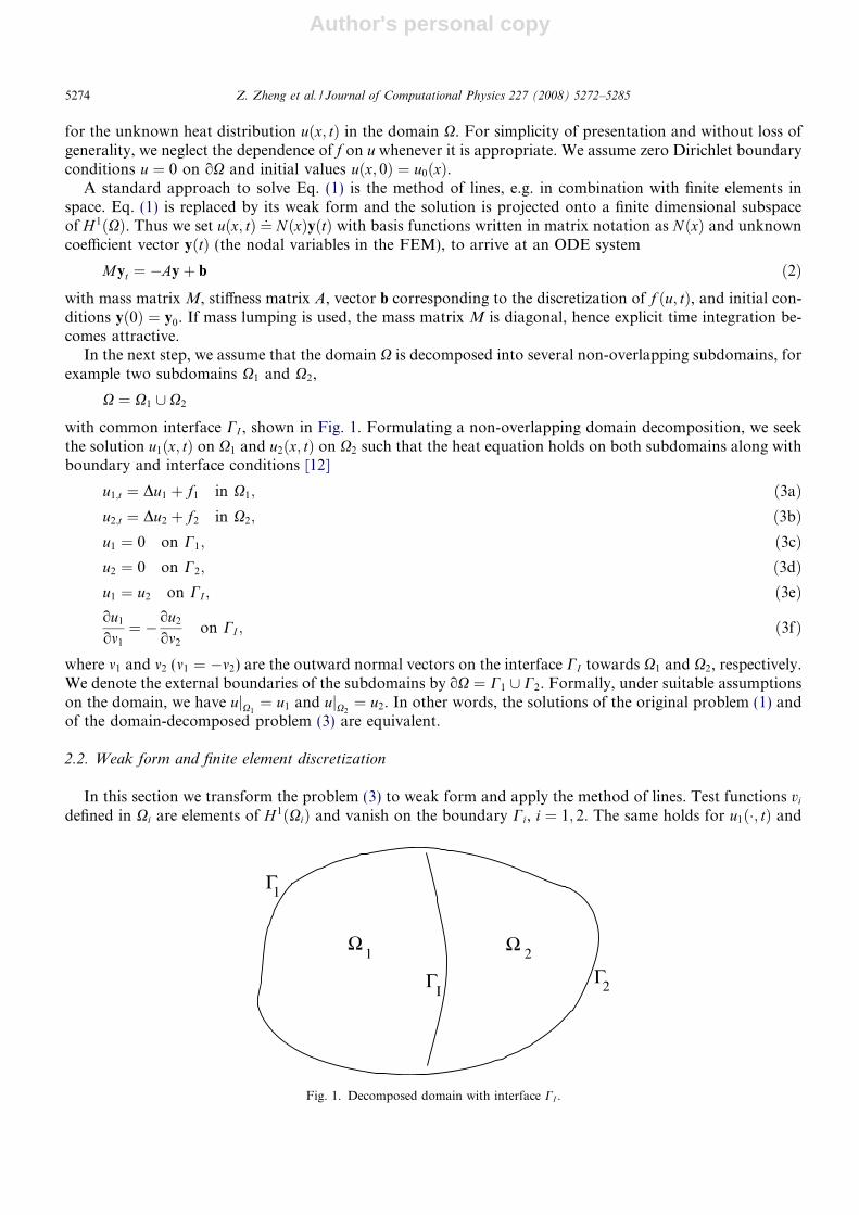
In the next step, we assume that the domain X is decomposed into several non-overlapping subdomains, forexample two subdomains X1 and X2,

X ¼ X1 [ X2

with common interface CI , shown in Fig. 1. Formulating a non-overlapping domain decomposition, we seekthe solution u1ðx; tÞ on X1 and u2ðx; tÞ on X2 such that the heat equation holds on both subdomains along withboundary and interface conditions [12]

u1;t ¼ Du1 þ f1 in X1; ð3aÞu2;t ¼ Du2 þ f2 in X2; ð3bÞu1 ¼ 0 on C1; ð3cÞu2 ¼ 0 on C2; ð3dÞu1 ¼ u2 on CI ; ð3eÞou1

om1

¼ � ou2

om2

on CI ; ð3fÞ

where m1 and m2 (m1 ¼ �m2) are the outward normal vectors on the interface CI towards X1 and X2, respectively.We denote the external boundaries of the subdomains by oX ¼ C1 [ C2. Formally, under suitable assumptionson the domain, we have ujX1

¼ u1 and ujX2¼ u2. In other words, the solutions of the original problem (1) and

of the domain-decomposed problem (3) are equivalent.

2.2. Weak form and finite element discretization

In this section we transform the problem (3) to weak form and apply the method of lines. Test functions vi

defined in Xi are elements of H 1ðXiÞ and vanish on the boundary Ci, i ¼ 1; 2. The same holds for u1ð�; tÞ and

Ω Ω

Γ Γ2

2

Γ

I

1

1

Fig. 1. Decomposed domain with interface CI .

5274 Z. Zheng et al. / Journal of Computational Physics 227 (2008) 5272–5285


u2ð�; tÞ at each instance of time t. On the interface CI , however, test functions and subdomain solutions do notvanish.

Application of Green’s theorem givesZXi

hrui;rviidx�Z

CI

vihrui; miids ¼ �Z

Xi

viDuidx; ð4Þ

and the weak form of the domain decomposition problem readsZX1

v1u1;tdxþZ

X1

hrv1;ru1idxþZ

CI

v1kds ¼Z

X1

v1f1dx for all v1; ð5aÞZ

X2

v2u2;tdxþZ

X2

hrv2;ru2idx�Z

CI

v2kds ¼Z

X1

v2f2dx for all v2; ð5bÞZ

CI

sðu1 � u2Þds ¼ 0 for all s; ð5cÞ

where v1, v2 and s are the test functions and

k ¼ �hru1; m1i ¼ hru2; m2i;defined on CI , is the Lagrange multiplier. We can thus view the Lagrange multiplier as a negative flux (or con-tact pressure) through the interface. By construction, the Neumann boundary condition (3f) is automaticallysatisfied. While the Dirichlet boundary conditions (3c) and (3d) have already been included in this formulationby the choice of v1 and v2, the interface condition u1 � u2 ¼ 0 is still present in the form of the weak constraintEq. (5c). The correct function space for the test function sðxÞ as well as for the Lagrange multiplier kðx; tÞ (withtime t frozen) would be the dual of the trace space H 1=2ðCIÞ.

Eq. (5) form a time-dependent saddle point problem or a partial differential-algebraic equation (PDAE).We can write the system in the abstract form as

ut þ Auþ BT k ¼ l;

Bu ¼ 0;

with u ¼ ðu1; u2Þ and corresponding operators A;B.As above in the unconstrained problem, finite dimensional subspaces are chosen to project the solution.

While the subdomain variables can be treated as before by a finite element ansatz, i.e., u1ðx; tÞ ¼: N 1ðxÞy1ðtÞ

and u2ðx; tÞ ¼: N 2ðxÞy2ðtÞ, the Lagrange multiplier k on the boundary requires special attention. Several possi-

bilities exist.

� Matching grids

If the grids for X1 and X2 match on the interface CI , the simplest choice is node-to-node constraints. Thismeans that the integral

RCI

sðu1 � u2Þds is replaced by the discrete sumP

ifsðu1 � u2Þgjxi, with the index i

running over all nodes on CI . In turn, we get the pointwise condition u1ðxi; tÞ ¼ u2ðxi; tÞ at all interfacenodes, and the Lagrange multiplier kðx; tÞ is discretized to a vector kðtÞ defined on the interface. One couldalso speak of a quadrature rule for the boundary integral.� Non-matching grids

Unlike the matching grids method, the non-matching grids method does not share nodes points betweensubdomains on the interface. The continuity between subdomains can be enforced by the Lagrange multi-plier method. However a special finite element space for the Lagrange multiplier must be chosen to stabilizethe domain decomposition problem.� Mortar element

The mortar method [40] is related to the above approach. It adds extra flexibility, in particular for non-matching grids.

We skip the details here and proceed with the resulting DAE system. All the above three methods reach thefollowing form:



M1y1;t ¼ �A1y1 þ b1 � BT1 k; ð6aÞ

M2y2;t ¼ �A2y2 þ b2 þ BT2 k; ð6bÞ

0 ¼ B1y1 � B2y2; ð6cÞor

Myt ¼ �Ayþ b� BT k; ð7aÞ0 ¼ By; ð7bÞ

where

M ¼M1 0

0 M2

� �; A ¼

A1 0

0 A2

� �; B ¼ ½B1 �B2 �; y ¼

y1

y2

� �; b ¼

b1

b2

� �:

Here, Mi and Ai are the mass and stiffness matrices for the subdomains, and the interface discretization leadsto constraint matrices B1 and B2. If the matrix B has full rank, Eq. (6) or Eq. (7) is a DAE of index 2 withblock-diagonal structure in the differential equations. Moreover, in the case of mass lumping, the mass matri-ces are diagonal. Hence explicit time integration becomes an option.

3. Explicit integration method

3.1. RKCP

In this section we introduce an explicit method for integrating Eq. (7). The RKC method [32–34], an explicitmethod designed for solving moderately stiff ODEs, has good stability properties while maintaining second-order accuracy. The real stability boundary of the RKC method increases quadratically with the number ofstages used. Hence it can use a much larger time step-size than traditional explicit Runge–Kutta methods.Combining the RKC method with the projection method [41,42], the RKCP method [35] was developed asan explicit method for solving DAEs, and it was shown that it preserves the zero-stability and absolute sta-bility properties of the RKC method. Thus we use the RKCP method to integrate the DAE (6). The RKCPalgorithm for integrating from fyn; kng at tn to fynþ1; knþ1g at tnþ1 can be formulated as follows:

Y0 ¼ yn;

F0 ¼ �M�1AY0 þM�1b�M�1BT kn;

Y1 ¼ Y0 þ ~l1DtF0;

Fj�1 ¼ �M�1AYj�1 þM�1b�M�1BT kn;

Yj ¼ ð1� lj � mjÞY0 þ ljYj�1 þ mjY

j�2 þ ~ljDtFj�1 þ ~cjDtF0; ðj ¼ 2; 3; . . . ; sÞ:Solve ðBM�1BT Þ/ ¼ BYs for /:

Update ynþ1 ¼ Ys �M�1BT /:

Update knþ1 ¼ kn þ 2/Dt:

ð8Þ

Here s is the number of Runge–Kutta stages and lj; ~lj; mj;~cj are the coefficients, determined for accuracy andstability of the method. What the above algorithm does is to use the RKC method to integrate Eq. (7a) from tn

to tnþ1 without regard to the constraint (7b) with a ‘‘frozen” k value at tn, i.e., kn. At the last stage of the RKCmethod, a projection procedure is performed to update y so that it satisfies the constraint (7b) and to update kn

to knþ1.Choosing the matching grids method, the continuity constraint (6c) reads

ðy1ÞCI� ðy2ÞCI

¼ 0; ð9Þ

where ðy1ÞCIand ðy2ÞCI

denote the interface nodes on CI of y1 and y2, respectively, and Eqs. (6a) and (6b) canbe elaborated as



M1y1;t ¼0 Zero Dirichlet boundary condition on C1

�A1y1 þ b1 Interior nodes in X1

�A1y1 þ b1 � k Interface nodes on CI

8><>: ; ð10Þ

and

M2y2;t ¼0 Zero Dirichlet boundary condition on C2

�A2y2 þ b2 Interior nodes in X2

�A2y2 þ b2 � k Interface nodes on CI

8><>: : ð11Þ

If additionally mass lumping techniques [39,43] are used in the finite element discretization, the mass matri-ces M1 and M2 can be replaced by diagonal matrices eM 1 and eM 2. Approximating a consistent mass matrix(M1, M2) with a lumped mass matrix ( eM 1, eM 2) will reduce the accuracy of the finite element method, howeverit is shown in [39] that the lumped mass matrix method converges with the order Oðh2Þ where h is the size ofthe finite elements. Thus the loss of spatial accuracy can be recovered by a refined grid. With a diagonal massmatrix, this method yields a fully explicit domain decomposition finite element method. For linear elements,~M1 (or eM 2) can be obtained simply by a row (or column) summation of M1 (or M2) and assigning the resultsonto the corresponding diagonal positions.

With the above simplifications, the projection step in scheme (8) is rewritten as

½ð eM�11 ÞCI

þ ð eM�12 ÞCI

�/ ¼ ðYs1ÞCI� ðYs

2ÞCI; ð12Þ

where ð�ÞCIdenotes the part of vectors or matrices defined on CI . Since both eM 1 and eM 2 are diagonal,

½ð eM�11 ÞCI

þ ð eM�12 ÞCI

� is also diagonal. It is trivial to solve Eq. (12). Hence the RKCP method applied to thedomain decomposition problem (6) is fully explicit. After solving the above equation for /, only the variableson the interface CI need to be updated,

ðynþ11 ÞCI

¼ ðYs1ÞCI� ð eM�1

1 ÞCI/; ð13Þ

ðynþ12 ÞCI

¼ ðYs2ÞCI� ð eM�1

2 ÞCI/; ð14Þ

knþ1 ¼ kn þ 2/Dt: ð15Þ

Overall, the RKCP method applied to the domain decomposition method is a fully explicit integrator, requir-ing no Newton iteration or linear system solver. At each time step, it consists of s explicit stages plus a finalprojection step which ‘‘synchronizes” the subdomains. It thus can be viewed as a fractional-step method whichincludes an explicit integration step and a final synchronization step.

The algorithm has an excellent potential for parallelization. In the integration step, the computation in eachsubdomain is totally independent, hence no communication between processors (subdomains) is needed. Inthe synchronization step, a continuity constraint must be satisfied on each interface which requires informa-tion exchange between the subdomains bordering on the same interface. In other words, the communication islocal, only across the interface between the two subdomains. Therefore the parallelization should be highlyscalable. Because the computation in each subdomain is totally independent, the method is also highly suitablefor multiphysics problems, where the model and/or the discretization may be different in different subdomains.

3.2. Stability analysis

In this section we analyze the zero-stability and the absolute stability properties of the RKCP methodapplied to the domain decomposition problem. We show that the method is zero-stable, and that, for stiffproblems, its stability region is at least as large as that of the corresponding RKC method.

Without loss of generality, we neglect the forcing term b in Eq. (7) and point out that the following analysisholds both for consistent and lumped mass matrices. One step integration of the ODE (7a) (with k frozen tokn) by the RKC method from tn to tnþ1 yields the intermediate solution [35]



ynþ1� ¼ P sð�DtM�1AÞyn þ ½I � P sð�DtM�1AÞ�ð�M�1AÞ�1M�1BT kn; ð16Þ

where P s is the stability polynomial of the RKC method, in the form of [33]

P sðzÞ ¼ 1þ zþ z2

2þXs

k¼3

Ckzk; ð17Þ

with Ck being the coefficients. Note here that M must be nonsingular for M�1 to exist, however A can be sin-gular, because ½I � P sð�DtM�1AÞ�ð�M�1AÞ�1 is a polynomial of A with non-negative exponents. The solutionynþ1 is obtained by a projection of ynþ1

� , written as

ynþ1 ¼ ðI � QÞynþ1� ; ð18Þ

where Q ¼ M�1BT ðBM�1BT Þ�1B. Denoting P sð�DtM�1AÞ as R, it is derived from Eq. (16) that

ynþ1� � yn

� ¼ Rðyn � yn�1Þ þ ðI � RÞð�M�1AÞ�1M�1BT ðkn � kn�1Þ: ð19ÞSince kn � kn�1 ¼ 2/

Dt, where / ¼ ðBM�1BT Þ�1Byn�, Eq. (19) is rewritten as

ynþ1� � yn

� ¼ RðI � QÞðyn� � yn�1

� Þ þ ðI � RÞ 2

Dtð�M�1AÞ�1Qy�n: ð20Þ

Let yn� ¼ vn þ wn, where vn ¼ ðI � QÞyn

� and wn ¼ Qyn�. We rewrite Eq. (20) as

vnþ1 þ wnþ1 � vn � wn ¼ Rðvn � vn�1Þ þ ðI � RÞ 2

Dtð�M�1AÞ�1

wn: ð21Þ

Consider the following two recurrences:

vnþ1 � vn ¼ Rðvn � vn�1Þ; ð22Þ

wnþ1 ¼ I þ ðI � RÞ 2

Dtð�M�1AÞ�1

� �wn: ð23Þ

The propagation matrices for the recurrences (22) and (23) are R and I þ ðI � RÞ 2Dt ð�M�1AÞ�1, respectively.

Expanding R ¼ P sð�DtM�1AÞ in the form of Eq. (17) and considering Dt small, we have

R ¼ I � DtM�1Aþ Dt2

2ðM�1AÞ2 þOðDt3Þ; ð24Þ

and thus

I þ ðI � RÞ 2

Dtð�M�1AÞ�1 ¼ �I þ DtM�1AþOðDt2Þ: ð25Þ

Zero-stability for recurrences (22) and (23), and hence for the RKCP method, is easily established, followingthe standard theory for numerical ODEs (e.g. [44]).

For absolute stability, let z ¼ Dtks, where ks denotes an eigenvalue of �M�1A. It can be shown that for z inthe stability region of the RKC method, i.e., kP sðzÞk 6 1, we always have �1 6 1�P sðzÞ

z 6 0. It follows that

�1 6 1þ 2 1�P sðzÞz 6 1. So we see that both recurrence (22) and recurrence (23) are stable. The sum of these

two recurrences, Eq. (21), is therefore stable.Stability analysis for a general projection method (implicit or explicit) can be found in [45]. It is mentioned

in [46] that mass lumping may affect the dissipation and dispersion properties of the classical time integrationmethods. It is correct that mass lumping affects the eigenvalues and thus leads to a somewhat different stabilityof the semi-discretized equations. In second-order problems (e.g. elasto-dynamics) where we have mostlyimaginary eigenvalues, this shift of the eigenvalues can be a severe difficulty, in particular if resonance frequen-cies for vibrational analysis play a role. However, in our first-order problem (parabolic case), we have mostlynegative real eigenvalues, and the mass lumping results in perturbations of decaying exponential functions. Asthe problem is stable anyway, the perturbations have no strong influence on the solution behavior. Yet they doinfluence the behavior of explicit integrators as the stability regions change somewhat. Thus the stability anal-ysis in this section can be extended to the lumped mass matrix case for the parabolic problems we consider.



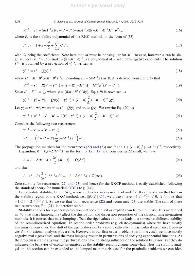
4. Numerical examples

4.1. 1D Brusselator problem

We first applied our method to the following 1D Brusselator problem on X ¼ ½0; 1�, using a finite differencediscretization:

ouot¼ D1

o2u

ox2þ a� ðbþ 1Þuþ u2v; ð26aÞ

ovot¼ D2

o2vox2þ bu� u2v; ð26bÞ

with boundary conditions

uð0; tÞ ¼ uð1; tÞ ¼ a;

vð0; tÞ ¼ vð1; tÞ ¼ b=a;

and initial conditions

uðx; 0Þ ¼ aþ xð1� xÞ;vðx; 0Þ ¼ b=aþ x2ð1� xÞ:

The problem domain X was decomposed into two non-overlapping subdomains X1 ¼ ½0; 0:5� and X2 ¼ ½0:5; 1�which in general may have different physics, namely different diffusion coefficients. The parameters were set asD1 ¼ D2 ¼ 1

40in X1, D1 ¼ D2 ¼ 1

800in X2, and a ¼ 0:6, b ¼ 2 in both X1 and X2. The problem domain was dis-

cretized in space with a second-order central difference for the diffusion term with spacing Dx ¼ 0:01. The timespan for the simulation is T ¼ ½0; 32�.

We implemented the adaptive Runge–Kutta–Chebyshev projection method (see [34] for the adaptive strat-egy) in Matlab scripts, called ARKCP and compared the results with the Matlab ODE solvers ODE15S,ODE45 and ODE23. In the case of the Matlab ODE solvers, the problem (26) was solved as an ODE bysemi-discretization in space. This can be viewed as an overlapping domain decomposition method wherethe interface continuity constraint is implemented as a boundary condition for each subdomain. We supplieda sparse Jacobian matrix for the implicit ODE solver ODE15S. In the tests shown in Table 1, the error is avector of u error and v error, computed as ku�urefk2

kurefk2, where u is the numerical solution and uref is the reference

solution which is computed by ODE15S with a very small error tolerance (RTOL=ATOL=1.0E�13). Underthe condition that each method yielded the same level of accuracy, we compared the computation times. Wesee that from Table 1 ARKCP is much faster than the explicit solvers ODE45 and ODE23, and is also fasterthan the implicit stiff solver ODE15S with the sparse Jacobian matrix. We note that such a PDE in one spatialdimension yields a tightly banded Jacobian matrix which can be factored and solved very efficiently inODE15S. That will no longer be the case in more than one spatial dimension.

Figs. 2 and 3 are plots of number of stages and step-size, respectively, chosen by the adaptive Runge–Kutta–Chebyshev projection (ARKCP) code. It is seen that within the error tolerance the code adjusts thetime step-size and thus the number of stages in response to the stiffness of the problem. Note that the solutionof the problem (26) is oscillatory with an approximate period of 12.

Table 1Numerical results for 1D Brusselator problem

Method RTOL ATOL Error CPU time (s)

ARKCP 1.0E�2 1.0E�2 [1.1E�3 1.2E�3] 1.8ODE15S 1.0E�3 1.0E�3 [2.2E�3 1.8E�3] 2.8ODE45 1.0E�2 1.0E�2 [7.6E�4 6.3E�4] 104.6ODE23 1.0E�2 1.0E�2 [1.4E�3 1.9E�3] 17.8



4.2. 2D Brusselator problem

We then applied our method to the 2D Brusselator problem (27) with a finite elment discretization,

ouot¼ D1

o2uox2þ o2u

oy2

� �þ a� ðbþ 1Þuþ u2v; ð27aÞ

ovot¼ D2

o2vox2þ o2v

oy2

� �þ bu� u2v; ð27bÞ

with boundary conditions

ouon¼ ov

on¼ 0;

at C1 and C2, and initial conditions

uðt ¼ 0Þ ¼ 0:5þ y;

vðt ¼ 0Þ ¼ 1þ 5x:

0 5 10 15 20 25 30 350

5

10

15

20

25mean(s)=13.4353

Time

Num

ber

of s

tage

s s

Fig. 2. Number of stages vs time for 1D Brusselator problem.

0 5 10 15 20 25 30 350

0.05

0.1

0.15

0.2

0.25

0.3

0.35mean(Δ t)=0.10095

Time

Tim

e st

ep—s

ize

Δt

Fig. 3. Time step-size vs time for 1D Brusselator problem.



Decomposed into two subdomains as shown in Fig. 4 and implementing the continuity constraint by Lagrangemultipliers, the problem (27) is formulated into a DAE in the form of Eq. (7). The parameters were set asD1 ¼ D2 ¼ 0:02, and a ¼ 1, b ¼ 3:4 in both subdomains. The time span for the simulation is T ¼ ½0; 8�.

We used COMSOL Multiphysics to implement the finite element model. After building the model in COM-SOL Multiphysics, we used the commands femlin and assemble to extract the mass matrix M, the stiffnessmatrix A and the constraint matrix B. We then applied the RKCP method to obtain the solution of the result-ing DAE. In the case of the Matlab ODE solvers, we first found the underlying ODE (this is basically the ODEwhich results from using the constraints of the DAE to eliminate the corresponding degrees of freedom [47]) ofthe DAE and solved that. We note that this may not be the most efficient way to solve the DAE, but it is thebest we can do if we want to use the Matlab ODE solvers. Linear Lagrange elements were used in the COM-SOL model.

The decomposed grids are shown in Fig. 4, in which the problem domain is discretized to 2014 elements and1048 nodes, decomposed into two subdomains.

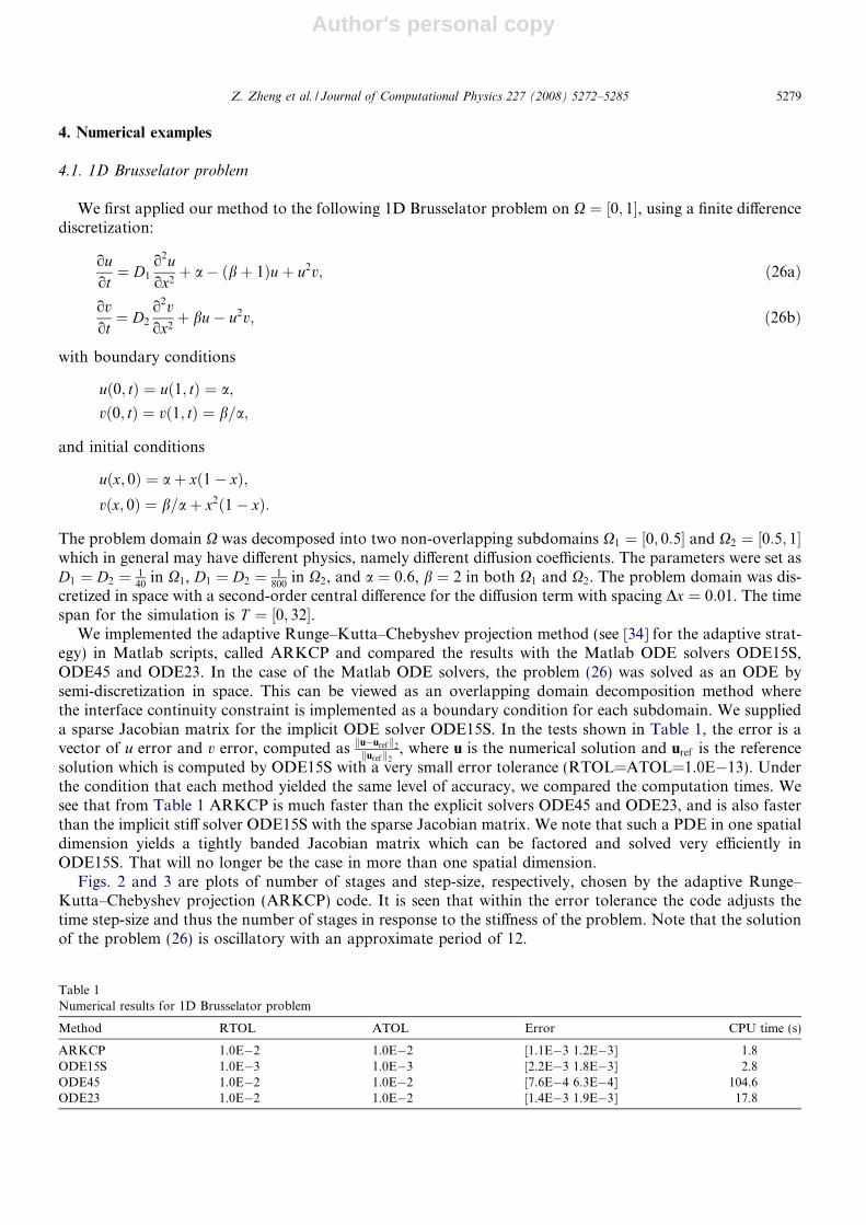
The numerical results with a consistent mass matrix and with a lumped mass matrix are shown in Tables 2and 3, respectively. The error in the tables was again computed as ku�urefk2

kurefk2, where u is the numerical solution

and uref is the reference solution which is the solution computed by COMSOL Multiphysics with a tight errortolerance. It is observed that with the same error tolerance, all the methods yield about the same level of accu-racy, but the ARKCP code is the most efficient.

The CPU time comparison with the Matlab solvers may not be the best proof of the performance of theRKCP method, since the problems used for our numerical tests are simple. However the numerical results

Fig. 4. Finite element grids for 2D Brusselator problem.

Table 2Numerical results for 2D Brusselator problem with consistent mass matrix


ARKCP 1.0E�2 1.0E�2 2.9E�2 113ODE15S 1.0E�2 1.0E�2 2.5E�2 276ODE45 1.0E�2 1.0E�2 1.4E�2 1005ODE23 1.0E�2 1.0E�2 1.4E�2 541



clearly show that the efficiency of the RKCP method is at least comparable to that of the implicit method. Wewould expect the relative advantages of the RKCP to increase, for larger more complex problems.

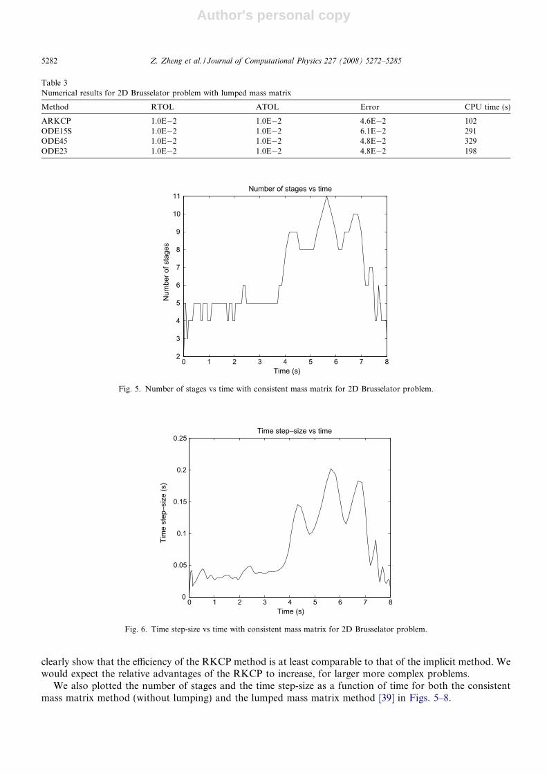
We also plotted the number of stages and the time step-size as a function of time for both the consistentmass matrix method (without lumping) and the lumped mass matrix method [39] in Figs. 5–8.

Table 3Numerical results for 2D Brusselator problem with lumped mass matrix


ARKCP 1.0E�2 1.0E�2 4.6E�2 102ODE15S 1.0E�2 1.0E�2 6.1E�2 291ODE45 1.0E�2 1.0E�2 4.8E�2 329ODE23 1.0E�2 1.0E�2 4.8E�2 198

0 1 2 3 4 5 6 7 82

3

4

5

6

7

8

9

10

11Number of stages vs time

Time (s)

Num

ber o

f sta

ges

Fig. 5. Number of stages vs time with consistent mass matrix for 2D Brusselator problem.

0 1 2 3 4 5 6 7 80

0.05

0.1

0.15

0.2

0.25Time step—size vs time

Time (s)

Tim

e st

ep—s

ize

(s)

Fig. 6. Time step-size vs time with consistent mass matrix for 2D Brusselator problem.



Our numerical experiments verify that the lumped mass matrix method converges to the second-order accu-racy, order Oðh2Þ where h is the finite element size.

5. Conclusions

In this paper a fully explicit, stabilized domain decomposition method for parabolic PDEs is presented.Through semi-discretization in space, the parabolic problem is formulated into a differential-algebraic equa-tion (DAE) system where the interface continuity constraints between subdomains are enforced by Lagrangemultipliers. The Runge–Kutta–Chebyshev projection (RKCP) method is used to integrate the DAE explicitlyand includes one projection per step to enforce the constraints. With mass lumping techniques and node-to-node matching grids, this method is fully explicit without solving any linear system. A stability analysis is pre-sented to show the extended stability property of the method. The method is straightforward to implementand to parallelize, with high scalability and low communication. Numerical results demonstrate that themethod has excellent performance.

0 1 2 3 4 5 6 7 82

3

4

5

6

7

8

9

10

11Number of stages vs time

Time (s)

Num

ber o

f sta

ges

Fig. 7. Number of stages vs time with lumped mass matrix for 2D Brusselator problem.

0 1 2 3 4 5 6 7 80

0.1

0.2

0.3

0.4

0.5

0.6

0.7Time step—size vs time

Time (s)

Tim

e st

ep—s

ize

(s)

Fig. 8. Time step-size vs time with lumped mass matrix for 2D Brusselator problem.



References

[1] H.A. Schwarz, Gesammelte Mathematicsche Abhandlungen, Springer-Verlag, 1890, vol. 2, p. 133.[2] M. Dryja, An additive Schwarz algorithm for two- and three-dimensional finite element elliptic problems, in: T.F. Chan, R.

Glowinski, J. Periaux, O. Widlund (Eds.), Proceedings of the Second International Symposium on Domain Decomposition Methodsfor Partial Differential Equations, SIAM, Philadelphia, PA, 1989, p. 168.

[3] P.E. Bjørstad, M. Skogen, Domain decomposition algorithms of Schwarz type, designed for massively parallel computers, in: D.E.Keyes, T.F. Chan, G.A. Meurant, J.S. Scroggs, R.G. Voigt (Eds.), Proceedings of the Fifth International Symposium on DomainDecomposition Methods for Partial Differential Equations, SIAM, Philadelphia, PA, 1992, p. 362.

[4] X.C. Cai, Additive Schwarz algorithms for parabolic convection–diffusion equations, Numer. Math. 60 (1) (1991) 41.[5] X.C. Cai, O. Widlund, Multiplicative Schwarz algorithms for nonsymmetric and indefinite problems, SIAM J. Numer. Anal. 30

(1993) 936.[6] X.C. Cai, Multiplicative Schwarz algorithms for parabolic problems, SIAM J. Sci. Comput. 15 (1994) 587.[7] X. Zhang, Multilevel Schwarz methods, Numer. Math. 63 (4) (1992) 521.[8] T.P. Mathew, Schwarz alternating and iterative refinement methods for mixed formulations of elliptic problems, part I: Algorithms

and numerical results, Numer. Math. 65 (4) (1993) 445.[9] P.E. Bjørstad, O.B. Widlund, Iterative methods for the solution of elliptic problems on regions partitioned into substructures, SIAM

J. Numer. Anal. 10 (5) (1986) 1053.[10] J.H. Bramble, J.E. Pasciak, A.H. Schatz, An iterative method for elliptic problems on regions partitioned into substructures, Math.

Comp. 46 (173) (1986) 361.[11] D. Funaro, A. Quarteroni, P. Zanolli, An iterative procedure with interface relaxation for domain decomposition methods, SIAM J.

Numer. Anal. 10 (5) (1988) 1053.[12] A. Toselli, O. Widlund, Domain Decomposition Methods – Algorithms and Theory, Springer, 2005.[13] J.F. Bourgat, R. Glowinski, P.L. Tallec, M. Vidrascu, Variational formulation and algorithm for trace operator in domain

decomposition calculations, in: T.F. Chan, R. Glowinski, J. Periaux, O. Widlund (Eds.), Proceedings of the Second InternationalSymposium on Domain Decomposition Methods for Partial Differential Equations, SIAM, Philadelphia, PA, 1989.

[14] Y.D. Roeck, P.L. Tallec, Analysis and test of a local domain decomposition preconditioner, in: R. Glowinski, Y.A. Kuznetsov, G.A.Meurant, J. Periaux, O. Widlund (Eds.), Proceedings of the Fourth International Symposium on Domain Decomposition Methodsfor Partial Differential Equations, SIAM, Philadelphia, PA, 1991.

[15] P.L. Tallec, Y.D. Roeck, M. Vidrascu, Domain decomposition methods for large linearly elliptic three-dimensional problems, J.Comput. Appl. Math. 34 (1) (1991) 93.

[16] J. Xu, J. Zou, Some nonoverlapping domain decomposition methods, SIAM Rev. 40 (4) (1998) 857.[17] C. Farhat, F.X. Roux, A method of finite element tearing and interconnecting and its parallel solution algorithm, Int. J. Numer.

Meth. Eng. 32 (1991) 1205.[18] J. Mandel, R. Tezaur, C. Farhat, An optimal Lagrange multiplier based domain decomposition method for plate bending problems,

Technical Report UCD-CCM-061, Center for Computational Mathematics, University of Colorado at Denver, 1995.[19] M. Lesoinne, K. Pierson, An efficient FETI implementation on distributed shared memory machines with independent numbers of

subdomains and processors, Contemp. Math. 218 (1998) 318.[20] A. Klawonn, O.B. Widlund, A domain decomposition method with Lagrange multipliers for linear elasticity, in: C.H. Lai, P.E.

Bjørstad, M. Cross, O.B. Widlund (Eds.), Proceedings of the Eleventh International Conference on Domain Decomposition Methods,Greenwich, UK, 1998.

[21] R. Tezaur, Analysis of Lagrange Multiplier Based Domain Decomposition. PhD thesis, University of Colorado at Denver, 1998.[22] G. Lube, L. Muller, F.-C. Otto, A non-overlapping DDM of Robin-Robin type for parabolic problems, in: C.H. Lai, P.E. Bjørstad,

M. Cross, O.B. Widlund (Eds.), Proceedings of the Eleventh International Conference on Domain Decomposition Methods,Greenwich, UK, 1998.

[23] M. Israeli, L. Vozovoi, A. Averbuch, Parallelizing implicit algorithms for time dependent problems by parabolic domaindecomposition, J. Sci. Comput. 8 (1993) 151.

[24] M. Dryja, X. Tu, A domain decomposition discretization of parabolic problems, Technical Report 860, Courant Institute ofMathematical Sciences, New York University, 2005.

[25] A.A. Samarskii, P.N. Vabishchevich, Domain decomposition methods for parabolic problems, in: C.H. Lai, P.E. Bjørstad, M. Cross,O.B. Widlund (Eds.), Proceedings of the Eleventh International Conference on Domain Decomposition Methods, Greenwich, UK,1998.

[26] Y. Zhuang, X. Sun, Stabilized explicit–implicit domain decomposition methods for the numerical solution of parabolic equations,SIAM J. Sci. Comput. 24 (2002) 335.

[27] H. Shi, H. Liao, Unconditional stability of corrected explicit–implicit domain decomposition algorithms for parallel approximation ofheat equations, SIAM J. Numer. Anal. 44 (4) (2006) 1584.

[28] C.N. Dawson, Q. Du, T.F. Dupont, A finite difference domain decomposition algorithm for numerical solution of the heat equation,Math. Comput. 57 (195) (1991) 63.

[29] C.N. Dawson, T.F. Dupont, Explicit/implicit, conservative domain decomposition procedures for parabolic problems based onblock-centered finite differences, SIAM J. Numer. Anal. 31 (1994) 1045.

[30] J. Zhu, H. Qian, On an efficient parallel algorithm for solving time dependent partial differential equations, in: Proceedings of thePDPTA’98 International Conference, 1998, p. 394.



[31] Y. Jun, T.-Z. Mai, IPIC Domain decomposition algorithm for parabolic problems, Appl. Math. Comput. 177 (1) (2006) 352.[32] P.J. van der Houwen, B.P. Sommeijer, On the internal stability of explicit, m-stage Runge–Kutta methods for large m-values, Z.

Angew. Math. Mech. 60 (1980) 479.[33] J.G. Verwer, Explicit Runge–Kutta methods for parabolic differential equations, Appl. Numer. Math. 22 (1996) 359.[34] B.P. Sommeijer, L.F. Shampine, J.G. Verwer, RKC: an explicit solver for parabolic PDEs, J. Comp. Appl. Math. 88 (1997) 315.[35] Z. Zheng, L.R. Petzold, Runge–Kutta–Chebyshev projection method, J. Comp. Phys. 219 (2006) 976.[36] J.G. Verwer, B.P. Sommeijer, W. Hundsdorfer, RKC time-stepping for advection–diffusion–reaction problems, J. Comp. Phys. 201

(2004) 61.[37] J.G. Verwer, B.P. Sommeijer, An implicit–explicit Runge–Kutta–Chebyshev scheme for diffusion–reaction equations, SIAM J. Sci.

Comput. 25 (2004) 1824.[38] R. Bermejo, M. El Amrani, A finite element semi-Lagrangian explicit Runge–Kutta–Chebyshev method for convection dominated

reaction–diffusion problems, J. Comput. Appl. Math. 154 (2003) 27.[39] S.R. Wu, Lumped mass matrix in explicit finite element method for transient dynamics of elasticity, Comput. Meth. Appl. Mech. Eng.

195 (2006) 5983.[40] F. Ben Belgacem, The mortar finite element method with Lagrange multipliers, Numer. Math. 84 (1999) 73.[41] A.J. Chorin, Numerical solution of the Navier–Stokes equations, Math. Comp. 22 (104) (1968) 745.[42] R. Temam, Sur l’approximation de la solution des equations de Navier–Stokes par la methode des pas fractionnaires (II), Arch. Rat.

Mech. Anal. 33 (1969) 377.[43] O. Botella, A high-order mass-lumping procedure for B-spline collocation method with application to incompressible flow

simulations, Int. J. Numer. Meth. Fluids 41 (2003) 1295.[44] U.M. Ascher, L.R. Petzold, Computer methods for ordinary differential equations and differential-algebraic equations, Soc. Ind.

Appl. Math. (1998).[45] Z. Zheng, L.R. Petzold, A framework for the analysis of second order projection methods, submitted for publication.[46] T.J.R. Hughes, The Finite Element Method: Linear Static and Dynamic Finite Element Analysis, Dover Publications, 2000.[47] U.M. Ascher, L.R. Petzold, Stability of computational methods for constrained dynamics systems, SIAM J. Sci. Statist. Comput. 14

(1993) 95.


Date post:	03-Feb-2022
Category:	Documents
Upload:	others
View:	1 times
Download:	0 times

Author's personal copy - UC Santa Barbara

Documents