AutoBridge: Coupling Coarse-Grained Floorplanning with Pipelining for High-Frequency HLS Design on Multi-Die FPGAsLicheng Guo1, Yuze Chi1, Jie Wang1, Jason Lau1, Weikang Qiao1, Ecenur Ustun2, Zhiru Zhang2, Jason Cong1

University of California Los Angeles1, Cornell Unversity2lcguo@ucla.eduhttps://github.com/Licheng-Guo/AutoBridge

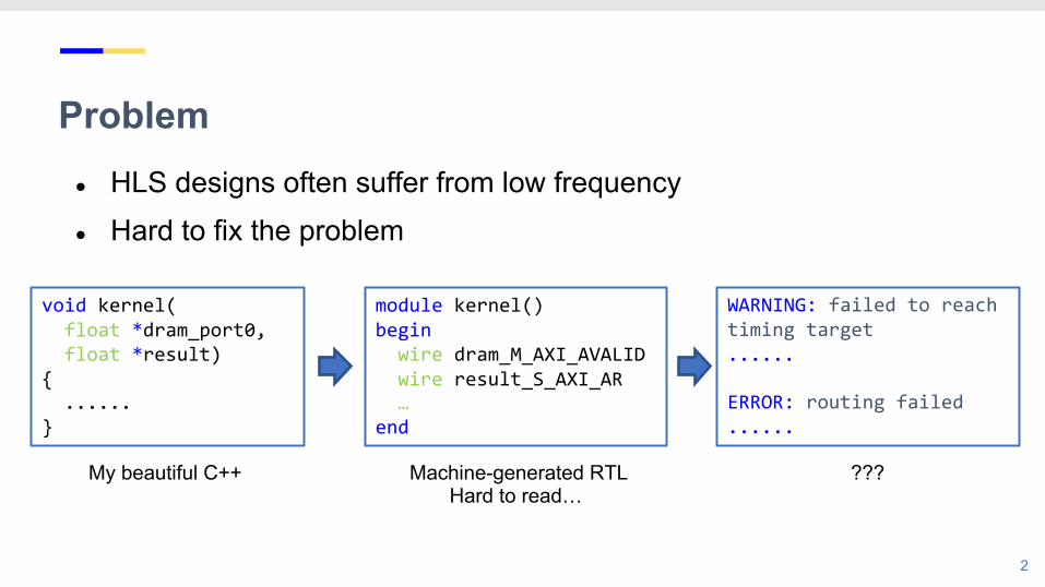
Problem● HLS designs often suffer from low frequency● Hard to fix the problem

2

void kernel(float *dram_port0,float *result)

{ ......

}

module kernel()begin

wire dram_M_AXI_AVALIDwire result_S_AXI_AR…

end

My beautiful C++ Machine-generated RTLHard to read…

WARNING: failed to reach timing target......

ERROR: routing failed......

???

Reason 1: Abstraction Gap● HLS has no physical layout information

○ How far will these two registers be apart?

○ How congested will the area be?

● Current HLS relies on inaccurate pre-characterized delay models

3

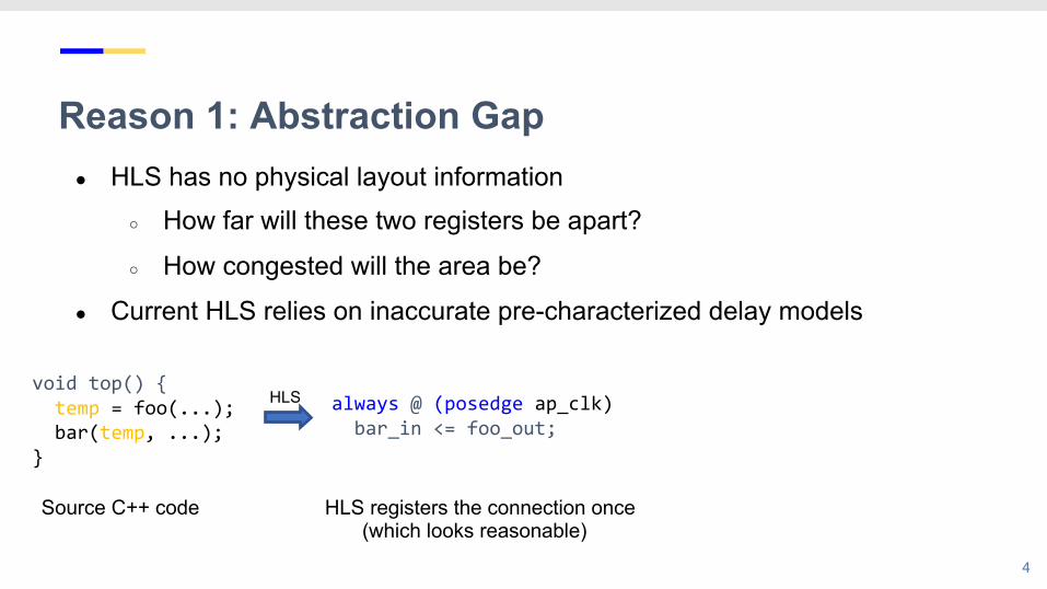
Reason 1: Abstraction Gap● HLS has no physical layout information

○ How far will these two registers be apart?

○ How congested will the area be?

● Current HLS relies on inaccurate pre-characterized delay models

4

always @ (posedge ap_clk)bar_in <= foo_out;

HLS registers the connection once(which looks reasonable)

void top() {temp = foo(...);bar(temp, ...);

}

Source C++ code

HLS

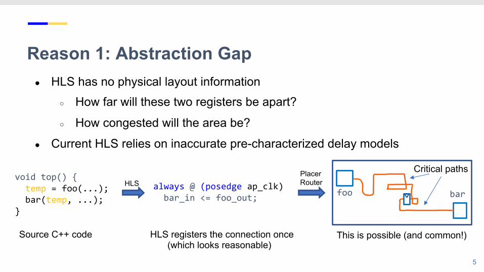
Reason 1: Abstraction Gap● HLS has no physical layout information

○ How far will these two registers be apart?

○ How congested will the area be?

● Current HLS relies on inaccurate pre-characterized delay models

5

always @ (posedge ap_clk)bar_in <= foo_out; foo bar

HLS registers the connection once(which looks reasonable)

Critical paths

This is possible (and common!)

void top() {temp = foo(...);bar(temp, ...);

}

Source C++ code

HLSPlacerRouter

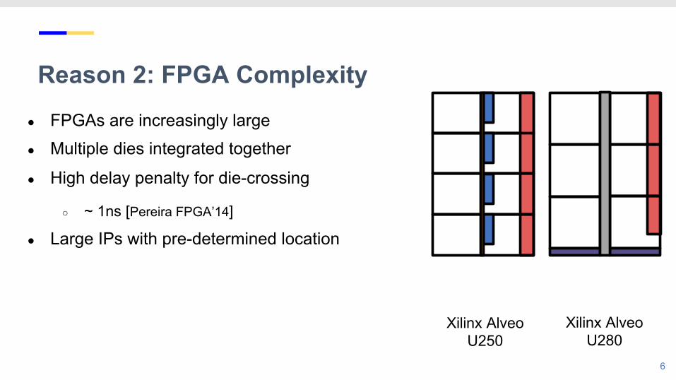
Reason 2: FPGA Complexity● FPGAs are increasingly large● Multiple dies integrated together

● High delay penalty for die-crossing

○ ~ 1ns [Pereira FPGA’14]

● Large IPs with pre-determined location

6

Xilinx AlveoU250

Xilinx AlveoU280

Reason 2: FPGA Complexity

7

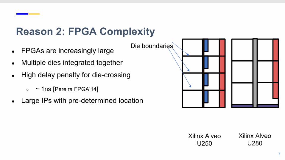
Die boundaries

Xilinx AlveoU250

Xilinx AlveoU280

● FPGAs are increasingly large● Multiple dies integrated together

● High delay penalty for die-crossing

○ ~ 1ns [Pereira FPGA’14]

● Large IPs with pre-determined location

Reason 2: FPGA Complexity● FPGAs are increasingly large● Multiple dies integrated together

● High delay penalty for die-crossing

○ ~ 1ns [Pereira FPGA’14]

● Large IPs with pre-determined location

8

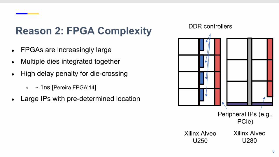
DDR controllers

Peripheral IPs (e.g., PCIe)

Xilinx AlveoU250

Xilinx AlveoU280

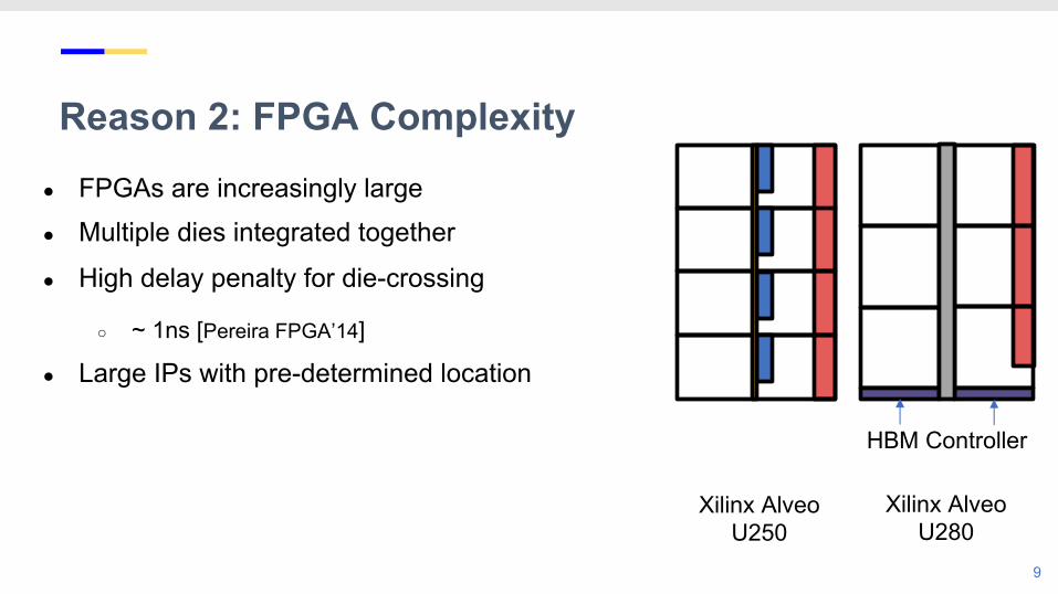
Reason 2: FPGA Complexity● FPGAs are increasingly large● Multiple dies integrated together

● High delay penalty for die-crossing

○ ~ 1ns [Pereira FPGA’14]

● Large IPs with pre-determined location

9

HBM Controller

Xilinx AlveoU250

Xilinx AlveoU280

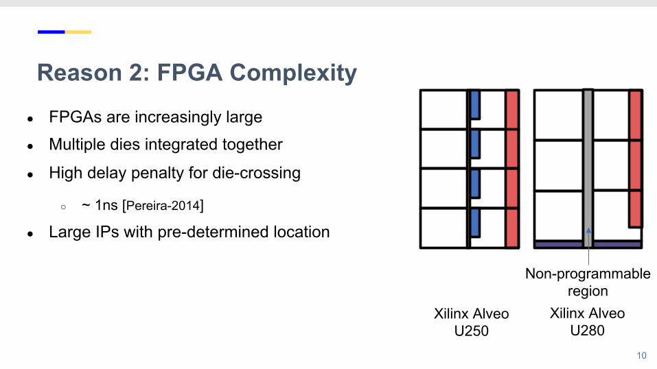
Reason 2: FPGA Complexity● FPGAs are increasingly large● Multiple dies integrated together

● High delay penalty for die-crossing

○ ~ 1ns [Pereira-2014]

● Large IPs with pre-determined location

10

Non-programmableregion

Xilinx AlveoU250

Xilinx AlveoU280

Reason 2: FPGA Complexity● HLS has limited consideration of those

physical barriers

11

Reason 2:● HLS has limited consideration of those

physical barriers

● Placer often needs to pack things together to reduce die crossing

○ Increase local congestion instead

12

Default Floorplan-Guided

Die 0

Die 1

Die 2

Die 3

Systolic arrayon U250

…

…

…

… … …

DDR-0

DDR-1

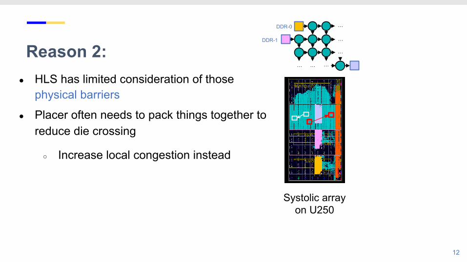
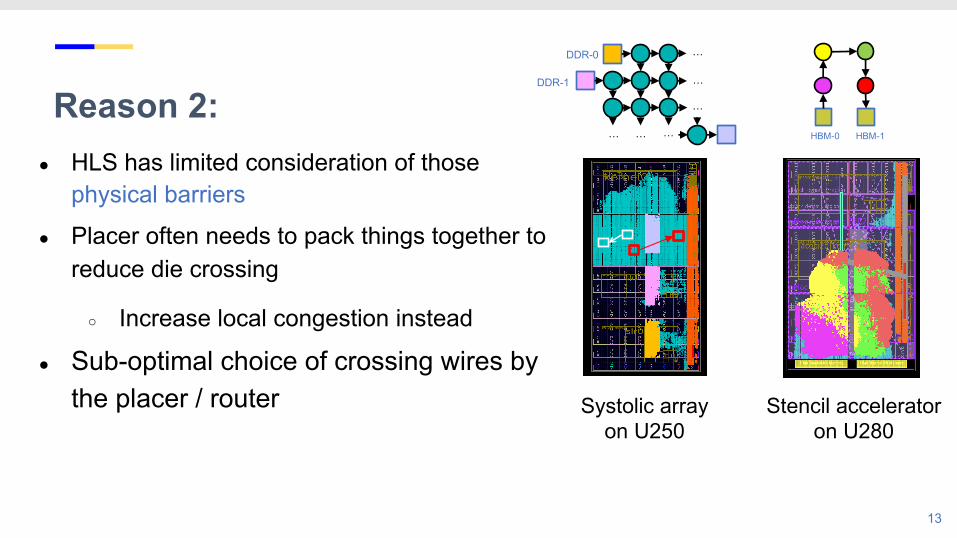
Reason 2:● HLS has limited consideration of those

physical barriers

● Placer often needs to pack things together to reduce die crossing

○ Increase local congestion instead

● Sub-optimal choice of crossing wires by the placer / router

13

Default Floorplan-Guided

Die 0

Die 1

Die 2

Die 3

Default Floorplan-GuidedSystolic array

on U250Stencil accelerator

on U280

HBM-0 HBM-1

…

…

…

… … …

DDR-0

DDR-1

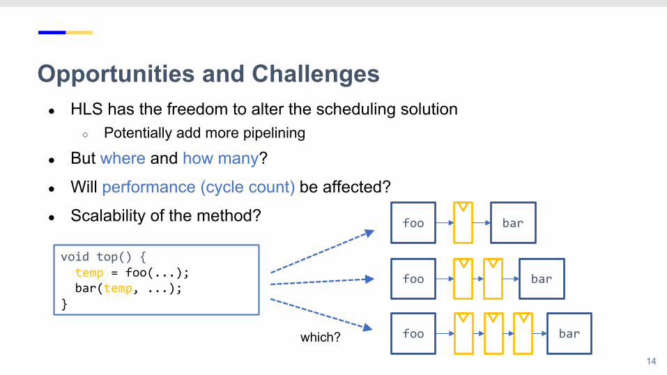
Opportunities and Challenges● HLS has the freedom to alter the scheduling solution

○ Potentially add more pipelining

● But where and how many?

● Will performance (cycle count) be affected?

● Scalability of the method?

14

void top() {temp = foo(...);bar(temp, ...);

}

foo bar

foo bar

foo barwhich?

Previous Attempts● Existing efforts focus on fine-grained delay model calibration

○ [Zheng-FPGA’12] Iteratively place & route to calibrate delay information for HLS

○ [Cong-2004] Placement-driven scheduling and binding

15

Previous Attempts● Existing efforts focus on fine-grained delay model calibration

○ [Zheng-FPGA’12] Iteratively place & route to calibrate delay information for HLS

○ [Cong-2004] Placement-driven scheduling and binding

● Not scalable, limited to tiny designs (only ~1000s of LUTs)

○ Our benchmarks can be 100X larger and many take days to implement

16

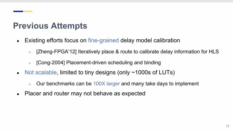
Previous Attempts● Existing efforts focus on fine-grained delay model calibration

○ [Zheng-FPGA’12] Iteratively place & route to calibrate delay information for HLS

○ [Cong-2004] Placement-driven scheduling and binding

● Not scalable, limited to tiny designs (only ~1000s of LUTs)

○ Our benchmarks can be 100X larger and many take days to implement

● Placer and router may not behave as expected

17

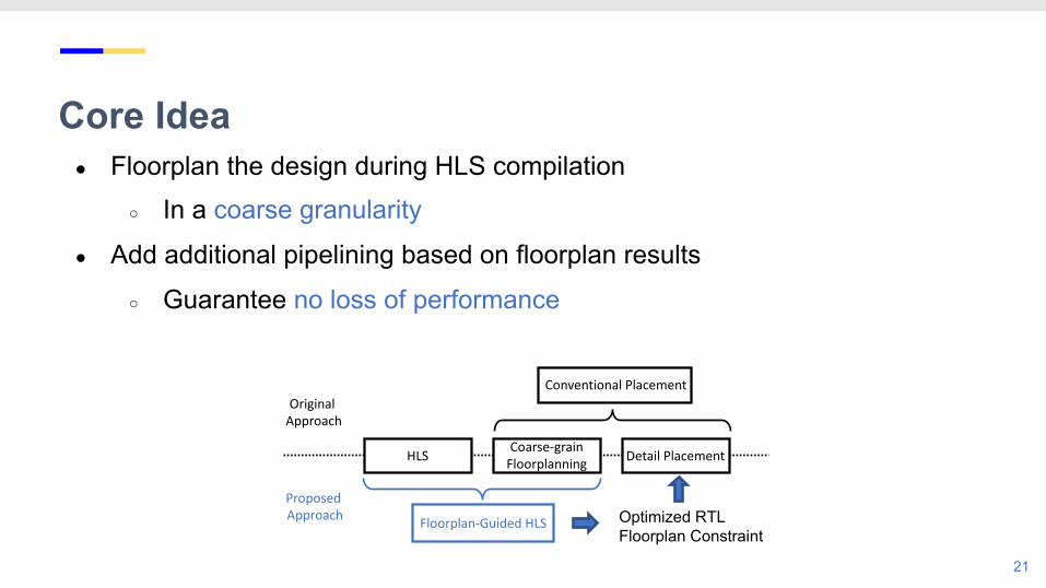
Core Idea● Floorplan the design during HLS compilation

○ In a coarse granularity

● Add additional pipelining based on floorplan results

○ Guarantee no loss of performance

18

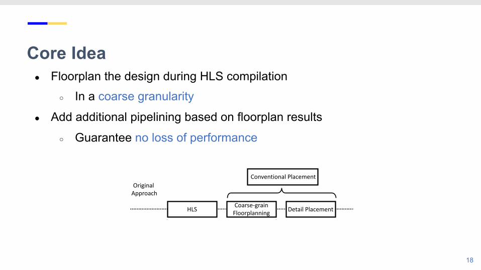
HLS Coarse-grain Floorplanning Detail Placement

Conventional Placement

Floorplan-Guided HLS

Original Approach

Proposed Approach

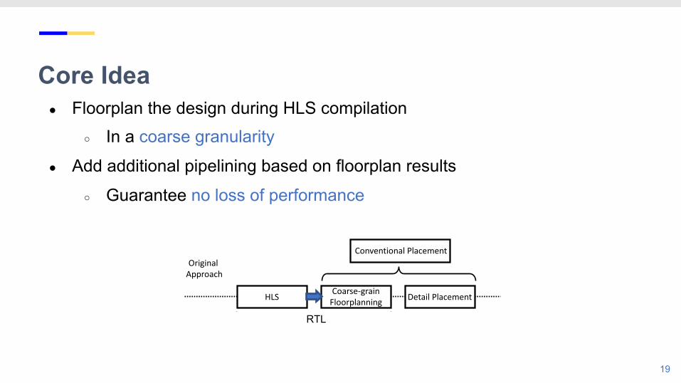
Core Idea● Floorplan the design during HLS compilation

○ In a coarse granularity

● Add additional pipelining based on floorplan results

○ Guarantee no loss of performance

19

HLS Coarse-grain Floorplanning Detail Placement

Conventional Placement

Floorplan-Guided HLS

Original Approach

Proposed Approach

RTL

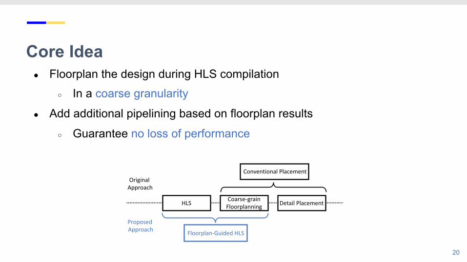
Core Idea● Floorplan the design during HLS compilation

○ In a coarse granularity

● Add additional pipelining based on floorplan results

○ Guarantee no loss of performance

20

HLS Coarse-grain Floorplanning Detail Placement

Conventional Placement

Floorplan-Guided HLS

Original Approach

Proposed Approach

Core Idea● Floorplan the design during HLS compilation

○ In a coarse granularity

● Add additional pipelining based on floorplan results

○ Guarantee no loss of performance

21

HLS Coarse-grain Floorplanning Detail Placement

Conventional Placement

Floorplan-Guided HLS

Original Approach

Proposed Approach Optimized RTL

Floorplan Constraint

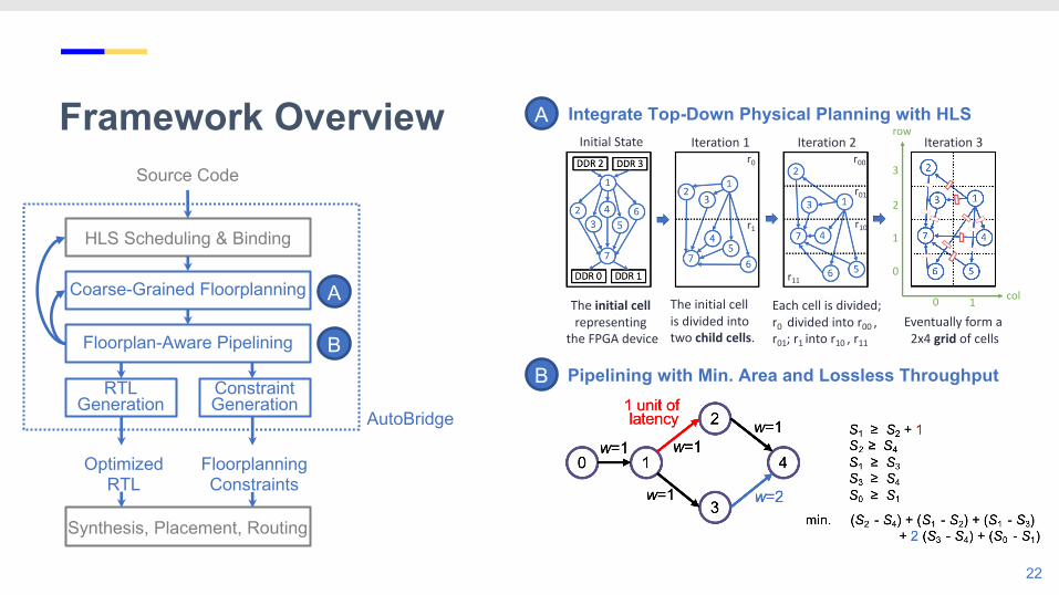
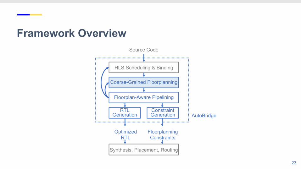
Framework Overview

22

HLS Scheduling & Binding

Coarse-Grained Floorplanning

Floorplan-Aware Pipelining

RTL Generation

Source Code

Synthesis, Placement, Routing

Constraint Generation

Optimized RTL

FloorplanningConstraints

AutoBridge

A

B

A

The initial cell representing

the FPGA device

The initial cell is divided into two child cells.

Eventually form a 2x4 grid of cells

Each cell is divided;r0 divided into r00 ,r01; r1 into r10 , r11

Initial State Iteration 1 Iteration 2 Iteration 3r0

r1

r00

r01

r10

r11

row

col0 1

0

1

2

3

B

Integrate Top-Down Physical Planning with HLS

Pipelining with Min. Area and Lossless Throughput

Framework Overview

23

HLS Scheduling & Binding

Coarse-Grained Floorplanning

Floorplan-Aware Pipelining

RTL Generation

Source Code

Synthesis, Placement, Routing

Constraint Generation

Optimized RTL

FloorplanningConstraints

AutoBridge

Coarse-Grained Floorplanning

24

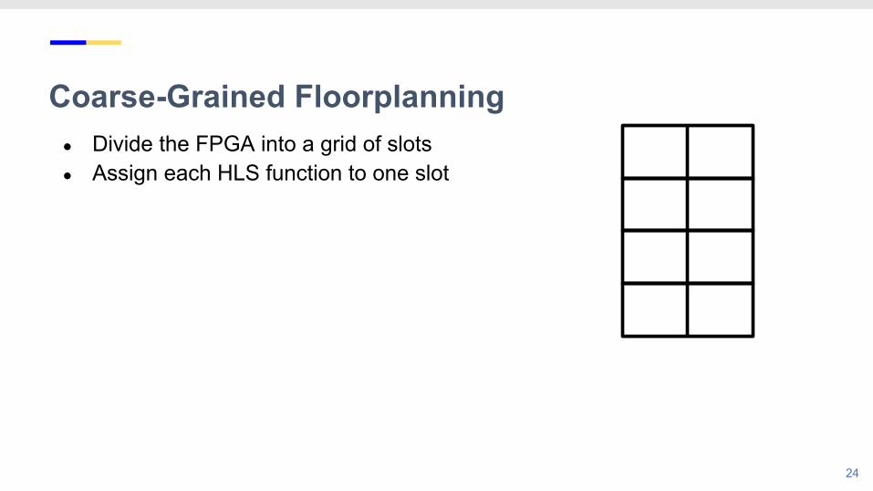
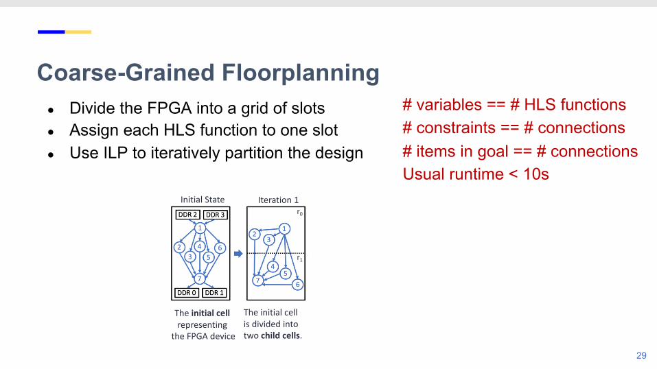
● Divide the FPGA into a grid of slots● Assign each HLS function to one slot

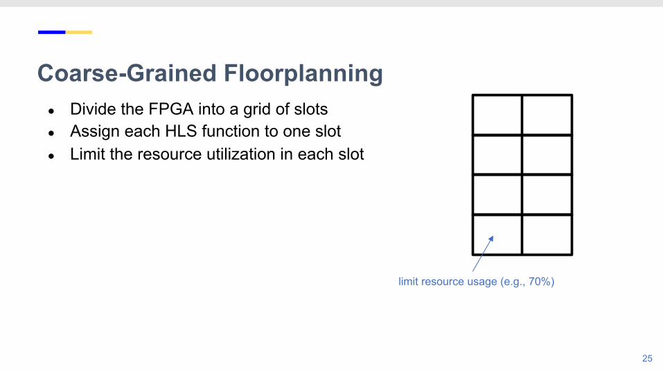
Coarse-Grained Floorplanning

25

● Divide the FPGA into a grid of slots● Assign each HLS function to one slot● Limit the resource utilization in each slot

limit resource usage (e.g., 70%)

Coarse-Grained Floorplanning

26

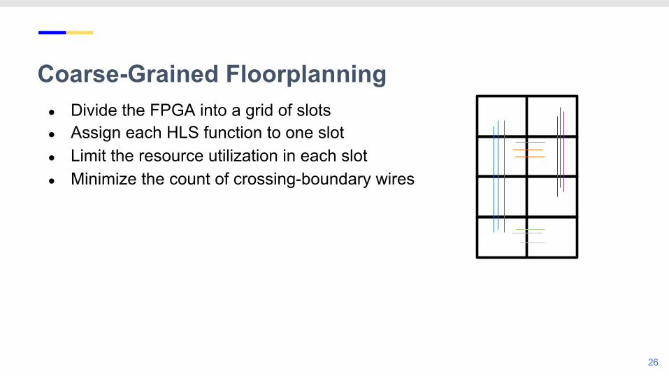
● Divide the FPGA into a grid of slots● Assign each HLS function to one slot● Limit the resource utilization in each slot● Minimize the count of crossing-boundary wires

Coarse-Grained Floorplanning

27

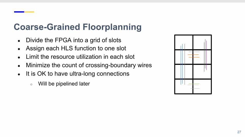
● Divide the FPGA into a grid of slots● Assign each HLS function to one slot● Limit the resource utilization in each slot● Minimize the count of crossing-boundary wires● It is OK to have ultra-long connections

○ Will be pipelined later

Coarse-Grained Floorplanning

28

The initial cell representing

the FPGA device

The initial cell is divided into two child cells.

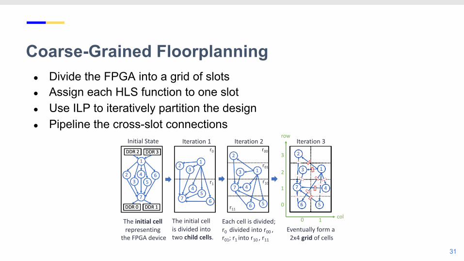
Eventually form a 2x4 grid of cells

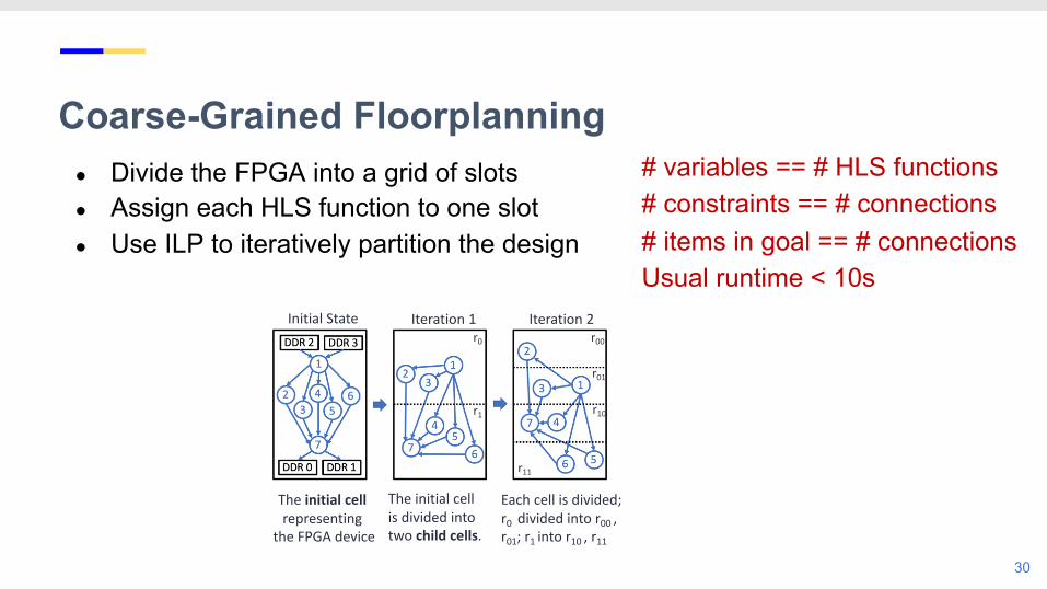
Each cell is divided;r0 divided into r00 ,r01; r1 into r10 , r11

Initial State Iteration 1 Iteration 2 Iteration 3r0

r1

r00

r01

r10

r11

row

col0 1

0

1

2

3

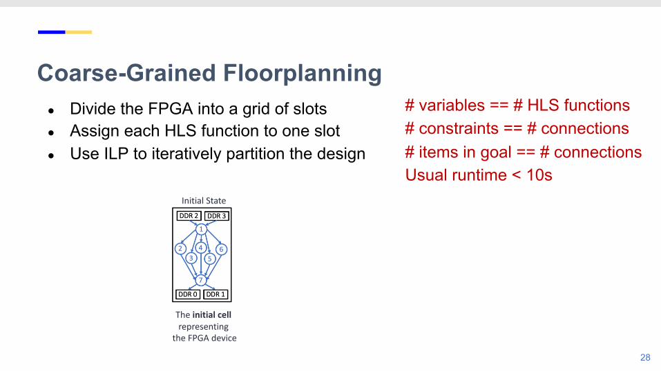
● Divide the FPGA into a grid of slots● Assign each HLS function to one slot● Use ILP to iteratively partition the design

# variables == # HLS functions# constraints == # connections# items in goal == # connectionsUsual runtime < 10s

Coarse-Grained Floorplanning

29

The initial cell representing

the FPGA device

The initial cell is divided into two child cells.

Eventually form a 2x4 grid of cells

Each cell is divided;r0 divided into r00 ,r01; r1 into r10 , r11

Initial State Iteration 1 Iteration 2 Iteration 3r0

r1

r00

r01

r10

r11

row

col0 1

0

1

2

3

● Divide the FPGA into a grid of slots● Assign each HLS function to one slot● Use ILP to iteratively partition the design

# variables == # HLS functions# constraints == # connections# items in goal == # connectionsUsual runtime < 10s

Coarse-Grained Floorplanning

30

The initial cell representing

the FPGA device

The initial cell is divided into two child cells.

Eventually form a 2x4 grid of cells

Each cell is divided;r0 divided into r00 ,r01; r1 into r10 , r11

Initial State Iteration 1 Iteration 2 Iteration 3r0

r1

r00

r01

r10

r11

row

col0 1

0

1

2

3

● Divide the FPGA into a grid of slots● Assign each HLS function to one slot● Use ILP to iteratively partition the design

# variables == # HLS functions# constraints == # connections# items in goal == # connectionsUsual runtime < 10s

Coarse-Grained Floorplanning

31

The initial cell representing

the FPGA device

The initial cell is divided into two child cells.

Eventually form a 2x4 grid of cells

Each cell is divided;r0 divided into r00 ,r01; r1 into r10 , r11

Initial State Iteration 1 Iteration 2 Iteration 3r0

r1

r00

r01

r10

r11

row

col0 1

0

1

2

3

● Divide the FPGA into a grid of slots● Assign each HLS function to one slot● Use ILP to iteratively partition the design● Pipeline the cross-slot connections

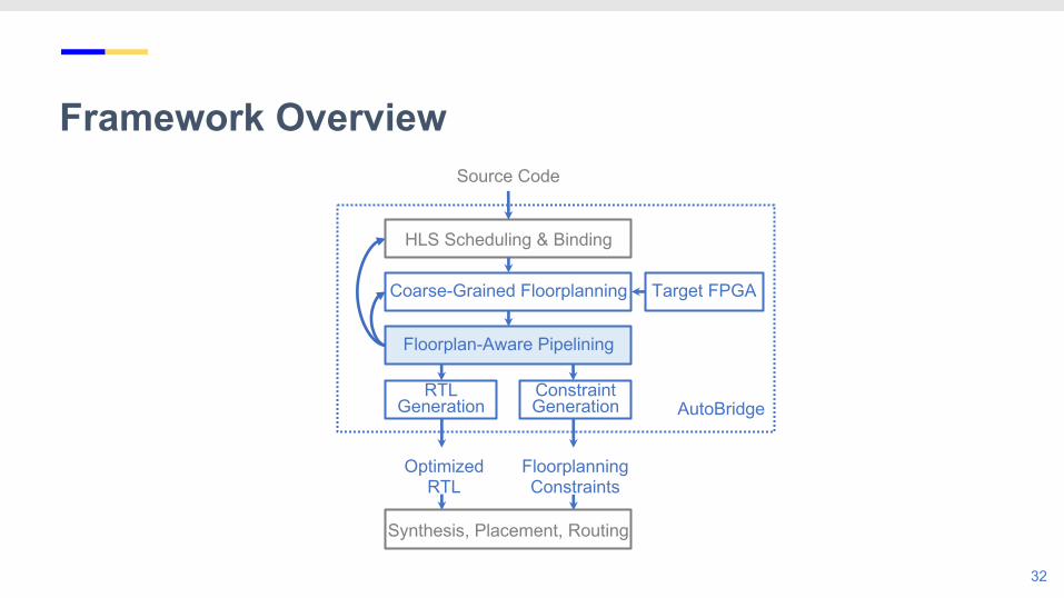
Framework Overview

32

HLS Scheduling & Binding

Coarse-Grained Floorplanning

Floorplan-Aware Pipelining

RTL Generation

Source Code

Synthesis, Placement, Routing

Constraint Generation

Target FPGA

Optimized RTL

FloorplanningConstraints

AutoBridge

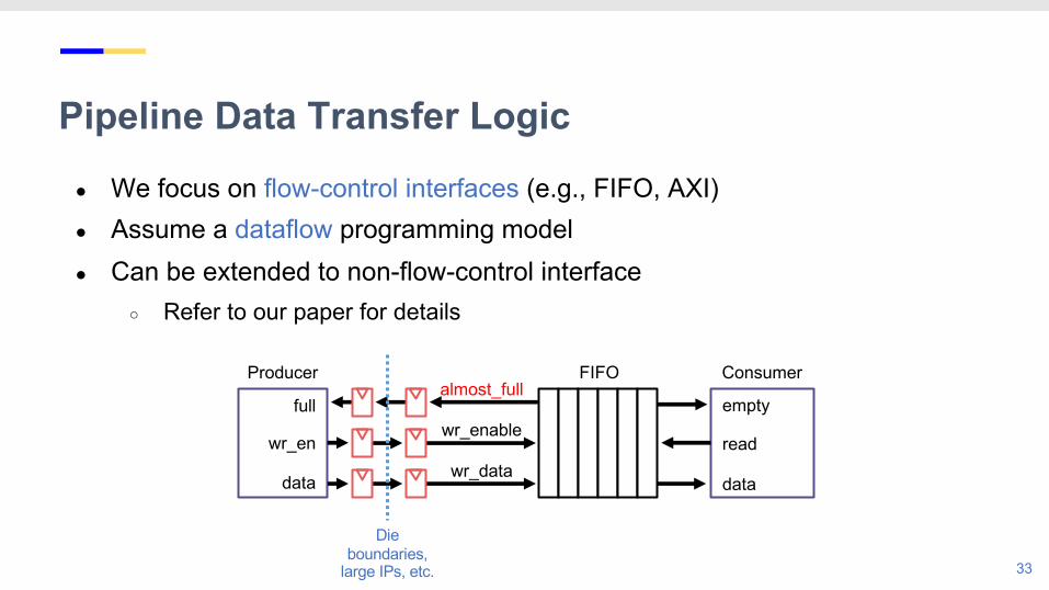
Pipeline Data Transfer Logic

33

almost_full

wr_enable

wr_data

full

wr_en

data

empty

read

data

Producer ConsumerFIFO

Die boundaries,

large IPs, etc.

● We focus on flow-control interfaces (e.g., FIFO, AXI)● Assume a dataflow programming model● Can be extended to non-flow-control interface

○ Refer to our paper for details

Address the Performance Concern● Focus on when modules communicate through FIFOs

○ Hard to statically analyze the impact of additional latency○ The additional latency may cause throughput decrease

34

Address the Performance Concern● Focus on when modules communicate through FIFOs

○ Hard to statically analyze the impact of additional latency○ The additional latency may cause throughput decrease

35

Note that each FIFO is being accessed by an arbitrary functionÞ Different from simplified model such as the Synchronous Data Flow (SDF)

Address the Performance Concern● Focus on when modules communicate through FIFOs

○ Hard to statically analyze the impact of additional latency○ The additional latency may cause throughput decrease

● Adapt cut-set pipelining ○ Add the same latency to all edges in a cut○ Equivalent to balancing the latency of reconvergent paths

36

1

e12

e13

e14

e15

e16

2

3

4

5

6

7

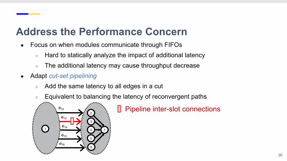
Pipeline inter-slot connections

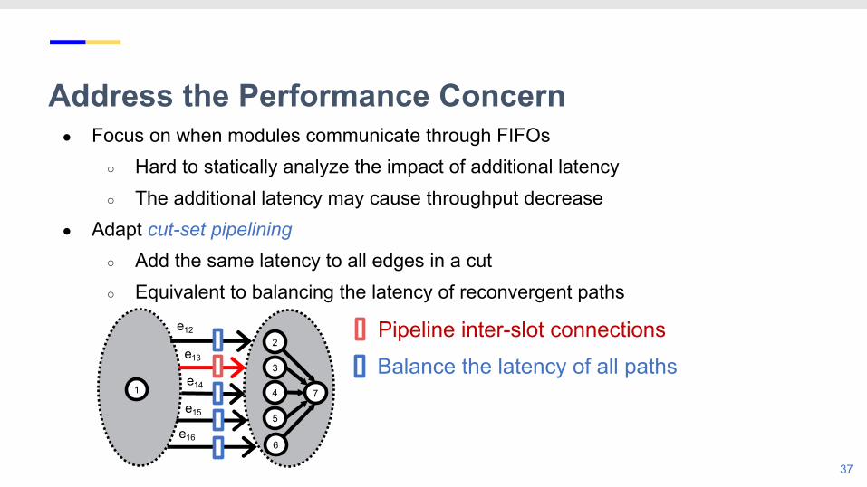
Address the Performance Concern● Focus on when modules communicate through FIFOs

○ Hard to statically analyze the impact of additional latency○ The additional latency may cause throughput decrease

● Adapt cut-set pipelining ○ Add the same latency to all edges in a cut○ Equivalent to balancing the latency of reconvergent paths

37

1

e12

e13

e14

e15

e16

2

3

4

5

6

7

Pipeline inter-slot connections Balance the latency of all paths

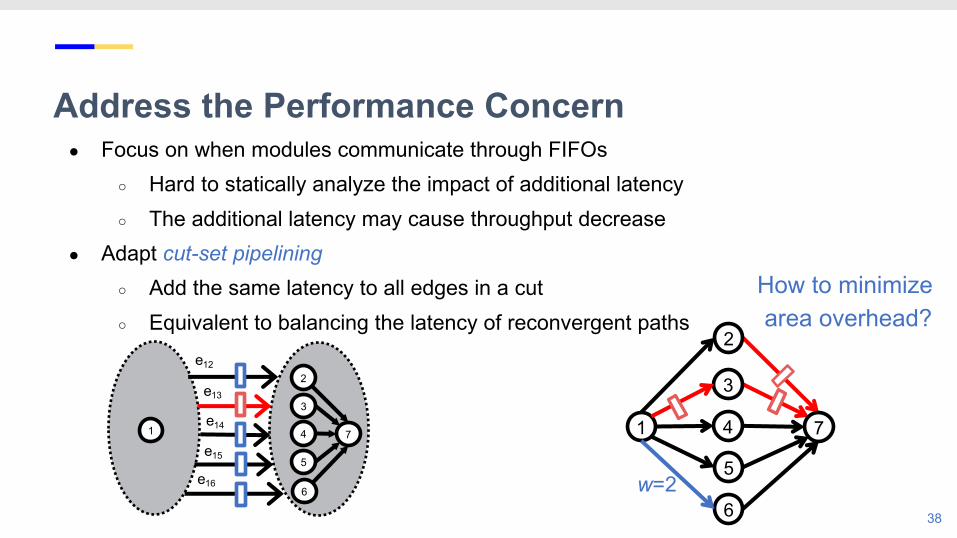
Address the Performance Concern● Focus on when modules communicate through FIFOs

○ Hard to statically analyze the impact of additional latency○ The additional latency may cause throughput decrease

● Adapt cut-set pipelining ○ Add the same latency to all edges in a cut○ Equivalent to balancing the latency of reconvergent paths

38

1

e12

e13

e14

e15

e16

2

3

4

5

6

7

How to minimize area overhead?

2

3

4

5

6

71

w=2

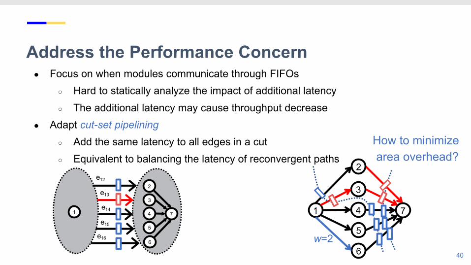
Address the Performance Concern● Focus on when modules communicate through FIFOs

○ Hard to statically analyze the impact of additional latency○ The additional latency may cause throughput decrease

● Adapt cut-set pipelining ○ Add the same latency to all edges in a cut○ Equivalent to balancing the latency of reconvergent paths

40

1

e12

e13

e14

e15

e16

2

3

4

5

6

7

2

3

4

5

6

71

w=2

How to minimize area overhead?

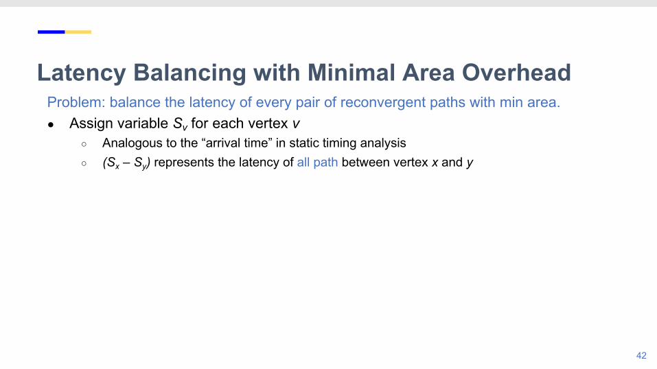
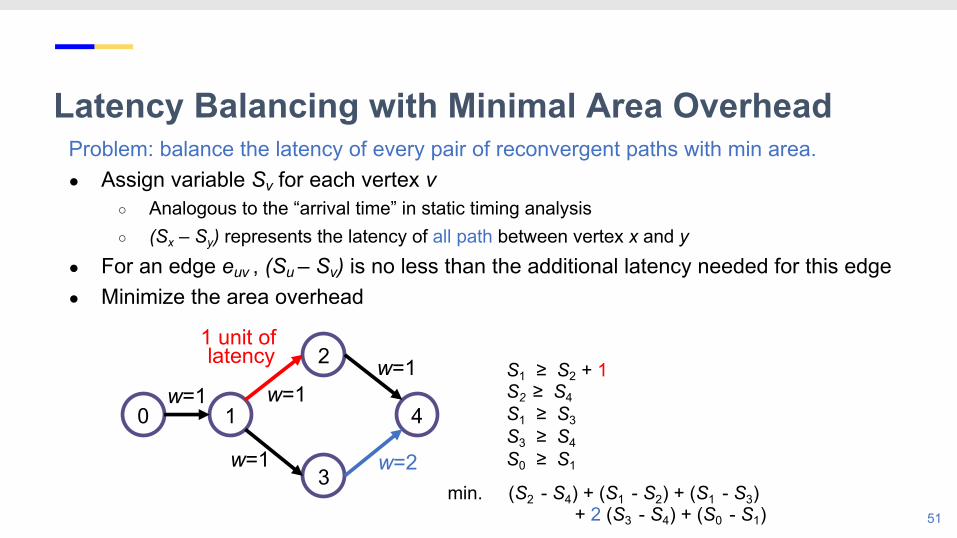
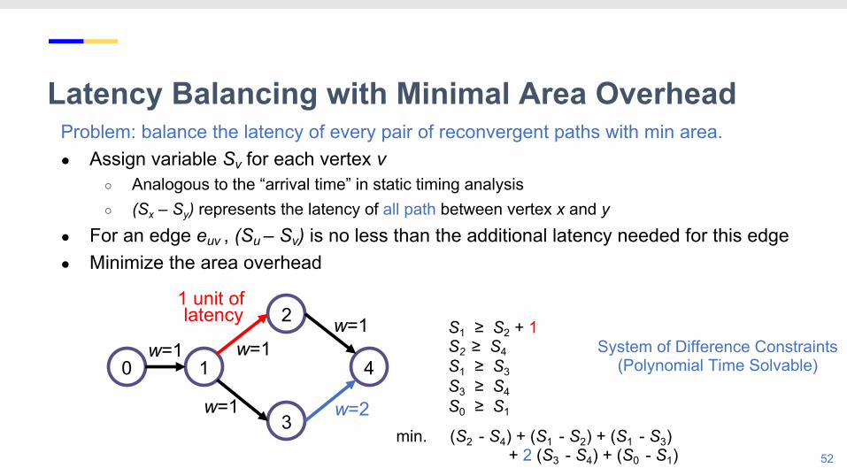
Latency Balancing with Minimal Area OverheadProblem: balance the latency of every pair of reconvergent paths with min area.

41

Latency Balancing with Minimal Area OverheadProblem: balance the latency of every pair of reconvergent paths with min area.● Assign variable Sv for each vertex v

○ Analogous to the “arrival time” in static timing analysis○ (Sx – Sy) represents the latency of all path between vertex x and y

42

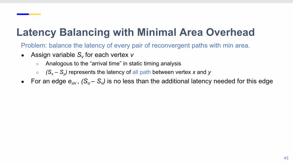
Latency Balancing with Minimal Area OverheadProblem: balance the latency of every pair of reconvergent paths with min area.● Assign variable Sv for each vertex v

○ Analogous to the “arrival time” in static timing analysis○ (Sx – Sy) represents the latency of all path between vertex x and y

● For an edge euv , (Su – Sv) is no less than the additional latency needed for this edge

43

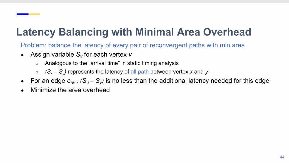
Latency Balancing with Minimal Area OverheadProblem: balance the latency of every pair of reconvergent paths with min area.● Assign variable Sv for each vertex v

○ Analogous to the “arrival time” in static timing analysis○ (Sx – Sy) represents the latency of all path between vertex x and y

● For an edge euv , (Su – Sv) is no less than the additional latency needed for this edge ● Minimize the area overhead

44

Latency Balancing with Minimal Area OverheadProblem: balance the latency of every pair of reconvergent paths with min area.● Assign variable Sv for each vertex v

○ Analogous to the “arrival time” in static timing analysis○ (Sx – Sy) represents the latency of all path between vertex x and y

● For an edge euv , (Su – Sv) is no less than the additional latency needed for this edge ● Minimize the area overhead

45

S1 ≥ S2 + 1S2 ≥ S4S1 ≥ S3S3 ≥ S4S0 ≥ S1

2

1

3

4

w=2w=1

0

1 unit of latency

w=1w=1w=1

min. (S2 - S4) + (S1 - S2) + (S1 - S3)+ 2 (S3 - S4) + (S0 - S1)

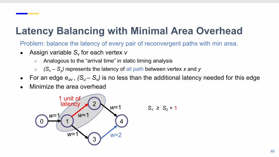
Latency Balancing with Minimal Area OverheadProblem: balance the latency of every pair of reconvergent paths with min area.● Assign variable Sv for each vertex v

○ Analogous to the “arrival time” in static timing analysis○ (Sx – Sy) represents the latency of all path between vertex x and y

● For an edge euv , (Su – Sv) is no less than the additional latency needed for this edge ● Minimize the area overhead

46

S1 ≥ S2 + 12

1

3

4

w=2w=1

0

1 unit of latency

w=1w=1w=1

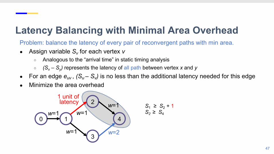
Latency Balancing with Minimal Area OverheadProblem: balance the latency of every pair of reconvergent paths with min area.● Assign variable Sv for each vertex v

○ Analogous to the “arrival time” in static timing analysis○ (Sx – Sy) represents the latency of all path between vertex x and y

● For an edge euv , (Su – Sv) is no less than the additional latency needed for this edge ● Minimize the area overhead

47

S1 ≥ S2 + 1S2 ≥ S4

2

1

3

4

w=2w=1

0

1 unit of latency

w=1w=1w=1

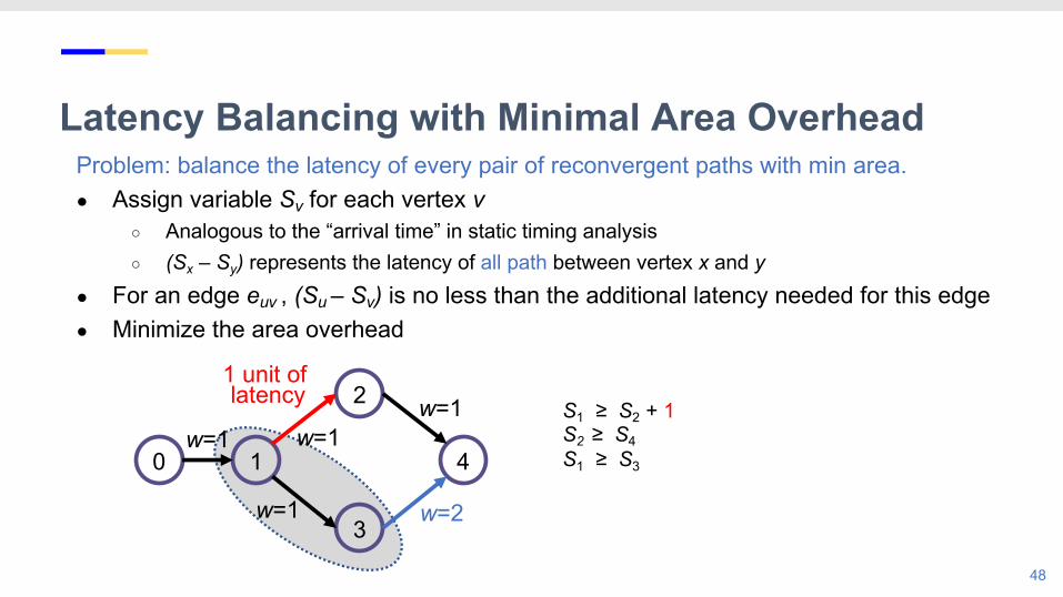
Latency Balancing with Minimal Area OverheadProblem: balance the latency of every pair of reconvergent paths with min area.● Assign variable Sv for each vertex v

○ Analogous to the “arrival time” in static timing analysis○ (Sx – Sy) represents the latency of all path between vertex x and y

● For an edge euv , (Su – Sv) is no less than the additional latency needed for this edge ● Minimize the area overhead

48

S1 ≥ S2 + 1S2 ≥ S4S1 ≥ S3

2

1

3

4

w=2w=1

0

1 unit of latency

w=1w=1w=1

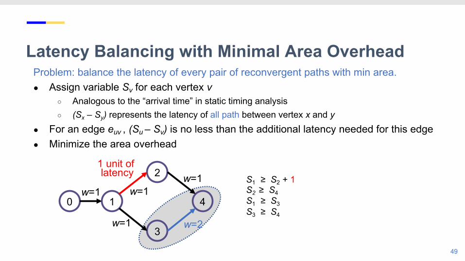
Latency Balancing with Minimal Area OverheadProblem: balance the latency of every pair of reconvergent paths with min area.● Assign variable Sv for each vertex v

○ Analogous to the “arrival time” in static timing analysis○ (Sx – Sy) represents the latency of all path between vertex x and y

● For an edge euv , (Su – Sv) is no less than the additional latency needed for this edge ● Minimize the area overhead

49

S1 ≥ S2 + 1S2 ≥ S4S1 ≥ S3S3 ≥ S4

2

1

3

4

w=2w=1

0

1 unit of latency

w=1w=1w=1

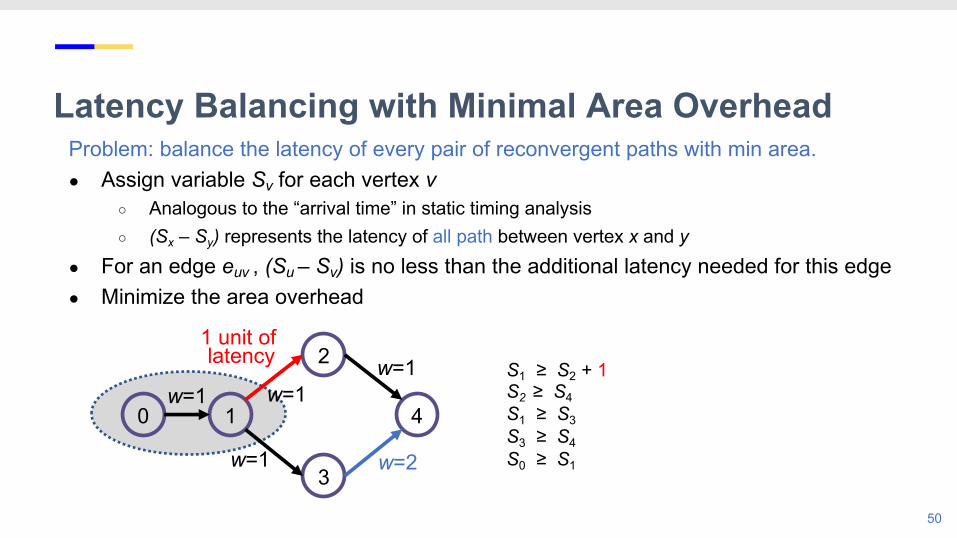
Latency Balancing with Minimal Area OverheadProblem: balance the latency of every pair of reconvergent paths with min area.● Assign variable Sv for each vertex v

○ Analogous to the “arrival time” in static timing analysis○ (Sx – Sy) represents the latency of all path between vertex x and y

● For an edge euv , (Su – Sv) is no less than the additional latency needed for this edge ● Minimize the area overhead

50

S1 ≥ S2 + 1S2 ≥ S4S1 ≥ S3S3 ≥ S4S0 ≥ S1

2

1

3

4

w=2w=1

0

1 unit of latency

w=1w=1w=1

Latency Balancing with Minimal Area OverheadProblem: balance the latency of every pair of reconvergent paths with min area.● Assign variable Sv for each vertex v

○ Analogous to the “arrival time” in static timing analysis○ (Sx – Sy) represents the latency of all path between vertex x and y

● For an edge euv , (Su – Sv) is no less than the additional latency needed for this edge ● Minimize the area overhead

51

S1 ≥ S2 + 1S2 ≥ S4S1 ≥ S3S3 ≥ S4S0 ≥ S1

2

1

3

4

w=2w=1

0

1 unit of latency

w=1w=1w=1

min. (S2 - S4) + (S1 - S2) + (S1 - S3)+ 2 (S3 - S4) + (S0 - S1)

Latency Balancing with Minimal Area OverheadProblem: balance the latency of every pair of reconvergent paths with min area.● Assign variable Sv for each vertex v

○ Analogous to the “arrival time” in static timing analysis○ (Sx – Sy) represents the latency of all path between vertex x and y

● For an edge euv , (Su – Sv) is no less than the additional latency needed for this edge ● Minimize the area overhead

52

S1 ≥ S2 + 1S2 ≥ S4S1 ≥ S3S3 ≥ S4S0 ≥ S1

2

1

3

4

w=2w=1

0

1 unit of latency

w=1w=1w=1

min. (S2 - S4) + (S1 - S2) + (S1 - S3)+ 2 (S3 - S4) + (S0 - S1)

System of Difference Constraints(Polynomial Time Solvable)

Benchmarks

53

… …

…

…

…

… … …

… … … …

Stencil Computation (Chi-ICCAD’18) Genome Sequencing (Guo-FCCM’19)

CNN (Wang-ICCAD’18) PageRank (Chi-Arcxiv’20)

Bucket Sort (Qiao-ISCA’20)

…

… … …… …

DDR-0 DDR-1 DDR-1DDR-0

HBM-0

HBM-1

HBM-7

HBM-8

HBM-9

HBM-15

DDR-0

DDR-1

DDR-2HBM-0

HBM-1

HBM-7

Gaussian Elimination (Wang-FPGA’21)

DDR-0

DDR-1DDR-2

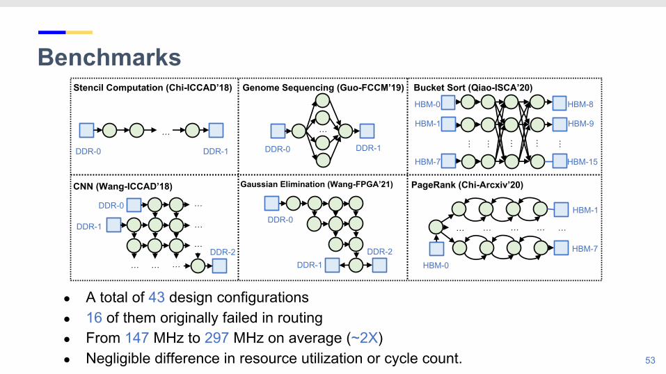
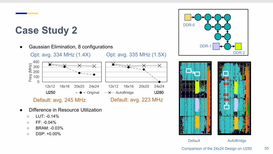
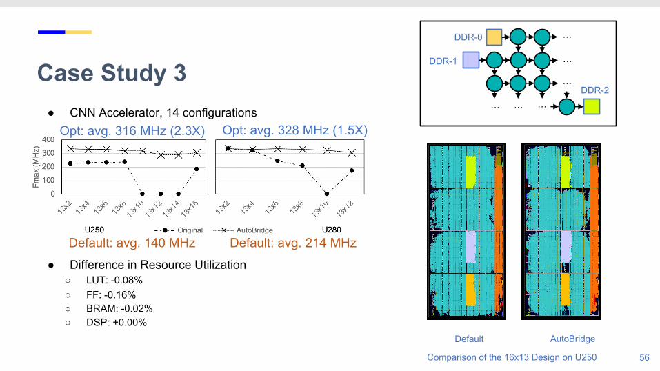
● A total of 43 design configurations ● 16 of them originally failed in routing ● From 147 MHz to 297 MHz on average (~2X)● Negligible difference in resource utilization or cycle count.

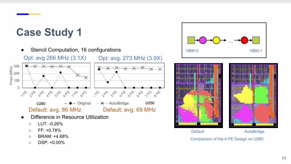
Case Study 1● Stencil Computation, 16 configurations

54

…

HBM-0 HBM-1

Default Floorplan-GuidedComparison of the 4-PE Design on U280

● Difference in Resource Utilization○ LUT: -0.26%○ FF: +0.78%○ BRAM: +4.68%○ DSP: +0.00%

AutoBridgeDefault

Default: avg. 86 MHz Default: avg. 69 MHz

Opt: avg 266 MHz (3.1X) Opt: avg. 273 MHz (3.9X)

Case Study 2● Gaussian Elimination, 8 configurations

55

DDR-0

DDR-1

DDR-2

● Difference in Resource Utilization○ LUT: -0.14%○ FF: -0.04%○ BRAM: -0.03%○ DSP: +0.00%

Comparison of the 24x24 Design on U250

AutoBridgeDefault

Default: avg. 245 MHz Default: avg. 223 MHz

Opt: avg. 334 MHz (1.4X) Opt: avg. 335 MHz (1.5X)

Case Study 3● CNN Accelerator, 14 configurations

56

…

…

…

… … …

DDR-0

DDR-1

DDR-2

● Difference in Resource Utilization○ LUT: -0.08%○ FF: -0.16%○ BRAM: -0.02%○ DSP: +0.00%

Comparison of the 16x13 Design on U250

AutoBridgeDefault

Default: avg. 140 MHz Default: avg. 214 MHz

Opt: avg. 316 MHz (2.3X) Opt: avg. 328 MHz (1.5X)

Impact of Pipelining and Floorplanning● Is it possible that only one of them is the key factor?

○ Baseline: (-) floorplanning, 8 slots (-) pipelining

○ AutoBridge: (+) floorplanning, 8 slots (-) pipelining

○ Case 1: (-) floorplanning (+) pipelining

○ Case 2: (+) floorplanning, 4 slots (neglect the DDRs) (-) pipelining

57Control Experiments Based on Systolic Arrays on U250

Projects Using AutoBridge● AutoSA: Polyhedral-Based Systolic Array Auto-Compilation

○ https://github.com/UCLA-VAST/AutoSA

● TAPA: Extending High-Level Synthesis for Task-Parallel Programs

○ https://github.com/Blaok/tapa

● Acceleration of Bayesian Network Inference (in submission)

● Acceleration of Single-Source-Shortest-Path algorithm (in submission)

58

https://github.com/Licheng-Guo/AutoBridge

Projects Using AutoBridge● AutoSA: Polyhedral-Based Systolic Array Auto-Compilation

○ https://github.com/UCLA-VAST/AutoSA

● TAPA: Extending High-Level Synthesis for Task-Parallel Programs

○ https://github.com/Blaok/tapa

● Acceleration of Bayesian Network Inference (in submission)

● Acceleration of Single-Source-Shortest-Path algorithm (in submission)

59

https://github.com/Licheng-Guo/AutoBridge

Thank You!

60