Solving the “false positives” problem in fraud predictionAutomated Data Science at an Industrial Scale

Roy Wedge and James Max Kanter and Kalyan VeeramachaneniData to AI Lab,

LIDS, MIT,Cambridge, MA-02139

Santiago Moral Rubio and Sergio Iglesias Perez†

Banco Bilbao Vizcaya Argentaria (BBVA)Madrid, Spain

AbstractIn this paper, we present an automated feature engineer-ing based approach to dramatically reduce false pos-itives in fraud prediction. False positives plague thefraud prediction industry. It is estimated that only 1 in 5declared as fraud are actually fraud and roughly 1 in ev-ery 6 customers have had a valid transaction declined inthe past year. To address this problem, we use the DeepFeature Synthesis algorithm to automatically derive be-havioral features based on the historical data of the cardassociated with a transaction. We generate 237 features(>100 behavioral patterns) for each transaction, and usea random forest to learn a classifier. We tested our ma-chine learning model on data from a large multinationalbank and compared it to their existing solution. On anunseen data of 1.852 million transactions, we were ableto reduce the false positives by 54% and provide a sav-ings of 190K euros. We also assess how to deploy thissolution, and whether it necessitates streaming compu-tation for real time scoring. We found that our solutioncan maintain similar benefits even when historical fea-tures are computed once every 7 days.

1. IntroductionDigital payment systems are enjoying growing popular-ity, and the companies that run them now have the abil-ity to store, as data, every interaction a customer haswith a payment system. Combined, these two devel-opments have led to a massive increase in the amountof available transaction data, and have made service

†Authors are the founding members of the Computer Sci-ence and Artificial Intelligence Laboratory (CSAIL), MIT’sCybsersecurity initiative.

providers better equipped than ever to handle the prob-lem of fraud detection.

Fraud detection problems are well-defined super-vised learning problems, and data scientists have longbeen applying machine learning to help solve themBrause, Langsdorf, and Hepp (1999); Ghosh and Reilly(1994). However, false positives still plague the indus-try (Pascual and Van Dyke, 2015). It is not uncommonto have false positive rates as high as 10-15% and haveonly 1 in 5 transactions declared as fraud be truly fraud(Pascual and Van Dyke, 2015). These high rates presentsignificant financial ramifications: many analysts havepointed out that false positives may be costing mer-chants more then fraud itself 1.

To mitigate this, most enterprises have adopted amulti-step process that combines work by human ana-lysts and machine learning models. This process usu-ally starts with a machine learning model generatinga risk score and combining it with expert-driven rulesto sift out potentially fraudulent transactions. The re-sulting alerts pop up in a 24/7 monitoring center, wherethey are examined and diagnosed by human analysts, asshown in Figure 1. This process can potentially reducethe false positive rate by 5% – but this improvementcomes only with high (and very costly) levels of humaninvolvement. Even with such systems in place, a largenumber of false positives remain.

In this paper, we present an improved machine learn-ing solution to drastically reduce the “false positives”in the fraud prediction industry. Such a solution willnot only have financial implications, but also reduce thealerts at the 24/7 control center, enabling security an-

1https://blog.riskified.com/true-cost-declined-orders/

arX

iv:1

710.

0770

9v1

[cs

.AI]

20

Oct

201

7

alysts to use their time more effectively, and thus de-livering the true promise of machine learning/artificialintelligence technologies.

We received a large, multi-year dataset from BBVA,containing 900 million transactions. We were also givenfraud reports that identified a very small subset of trans-actions as fraudulent. Our task was to develop a ma-chine learning solution that: (a) uses this rich transac-tional data in a transparent manner (no black box ap-proaches), (b) competes with the solution currently inuse by BBVA, and (c) is deployable, keeping in mindthe real-time requirements placed on the prediction sys-tem.

We would be remiss not to acknowledge the numer-ous machine learning solutions achieved by researchersand industry alike (more on this in Section 3.). However,the value of extracting patterns from historical data hasbeen only recently recognized as an important factor indeveloping these solutions – instead, the focus has gen-erally been on finding the best possible model given aset of features, and even after this , few studies focusedon extracting a handful of features. Recognizing the im-portance of feature engineering Domingos (2012) – inthis paper, we use an automated feature engineering ap-proach to generate hundreds of features to exploit theselarge caches of data and dramatically reduce the falsepositives.

2. Key findings and resultsKey to success is automated feature engineering:Having access to rich information about cards and cus-tomers exponentially increases the number of possiblefeatures we can generate. However, coming up withideas, manually writing software and extracting featurescan be time-consuming, and may require customizationeach time a new bank dataset is encountered. In thispaper, we use an automated method called deep featuresynthesis(DFS) to rapidly generate a rich set of featuresthat represent the patterns of use for a particular accoun-t/card. Examples of features generated by this approachare presented in Table 4.

As per our assessment, because we were able to per-form feature engineering automatically via Featuretoolsand machine learning tools, we were able to focus ourefforts and time on understanding the domain, evaluat-ing the machine learning solution for financial metrics(>60% of our time), and communicating our results.We imagine tools like these will also enable others tofocus on the real problems at hand, rather than becom-

ing caught up in the mechanics of generating a machinelearning solution.Deep feature synthesis obviates the need for stream-ing computing: While the deep feature synthesis al-gorithm can generate rich and complex features usinghistorical information, and these features achieve supe-rior accuracy when put through machine learning, it stillneeds to be able to do this in real time in order to feedthem to the model. In the commercial space, this hasprompted the development of streaming computing so-lutions.

But, what if we could compute these features onlyonce every t days instead? During the training phase,the abstractions in deep feature synthesis allow featuresto be computed with such a “delay,” and for theiraccuracy to be tested, all by setting a single parameter.For example, for a transaction that happened on August24th, we could use features that had been generated onAugust 10th. If accuracy is maintained, the implicationis that aggregate features need to be only computedonce every few days, obviating the need for streamingcomputing.

What did we achieve?DFS achieves a 91.4% increase in precision com-

pared to BBVA’s current solution. This comes out toa reduction of 155,870 false positives in our dataset – a54% reduction.

The DFS-based solution saves 190K euros over1.852 million transactions - a tiny fraction of the to-tal transactional volume. These savings are over 1.852million transactions, only a tiny fraction of BBVA’syearly total, meaning that the true annual savings willbe much larger.

We can compute features, once every 35 days andstill generate value Even when DFS features are onlycalculated once every 35 days, we are still able toachieve an improvement of 91.4% in precision. How-ever, we do lose 67K euros due to approximation, thusonly saving 123K total euros. This unique capabilitymakes DFS is a practically viable solution.

3. Related workFraud detection systems have existed since the late1990s. Initially, a limited ability to capture, storeand process data meant that these systems almost al-ways relied on expert-driven rules. These rules gener-ally checked for some basic attributes pertaining to the

Information type Attribute recordedVerification results

Card captures information about unique situations during card verification.Terminal captures information about unique situations during verification at a terminal.

About the locationTerminal can print/display messages

can change data on the cardmaximum pin length it can acceptserviced or nothow data is input into the terminal

Authentication device typemode

About the merchant unique idbank of the merchanttype of merchantcountry

About the card authorizerAbout the transaction amount

timestampcurrencypresence of a customer

Table 1: A transaction, represented by a number of attributes that detail every aspect of it. In this table, we are showing*only* a fraction of what is being recorded in addition to the amount, timestamp and currency for a transaction.These range from whether the customer was present physically for the transaction to whether the terminal where thetransaction happened was serviced recently or not. We categorize the available information into several categories.

transaction – for example, “Is the transaction amountgreater then a threshold?” or “Is the transaction hap-pening in a different country?” They were used to blocktransactions, and to seek confirmations from customersas to whether or not their accounts were being used cor-rectly.

Next, machine learning systems were developed toenhance the accuracy of these systems Brause, Langs-dorf, and Hepp (1999); Ghosh and Reilly (1994). Mostof the work done in this area emphasized the modelingaspect of the data science endeavor – that is, learning aclassifier. For example, Chan et al. (1999); Stolfo et al.(1997) present multiple classifiers and their accuracy.Citing the non-disclosure agreement, they do not revealthe fields in the data or the features they created. Addi-tionally, Chan et al. (1999) present a solution using onlytransactional features, as information about their data isunavailable.

Starting with Shen, Tong, and Deng (2007), re-searchers have started to create small sets of hand-crafted features, aggregating historical transactional in-

formation Bhattacharyya et al. (2011); Panigrahi et al.(2009). Whitrow et al. (2009) emphasize the impor-tance of aggregate features in improving accuracy. Inmost of these studies, aggregate features are gener-ated by aggregating transactional information from theimmediate past of the transaction under consideration.These are features like “number of transactions thathappened on the same day”, or “amount of time elapsedsince the last transaction”.

Fraud detection systems require instantaneous re-sponses in order to be effective. This places limitson real-time computation, as well as on the amountof data that can be processed. To enable predictionswithin these limitations, the aggregate features usedin these systems necessitate a streaming computationalparadigm in production 2, 3 Carcillo et al. (2017). As wewill show in this paper, however, aggregate summaries

2https://mapr.com/blog/real-time-credit-card-fraud-detection-apache-spark-and-event-streaming/

3https://www.research.ibm.com/foiling-financial-fraud.shtml

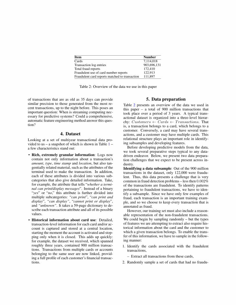
Item NumberCards 7,114,018Transaction log entries 903,696,131Total fraud reports 172,410Fraudulent use of card number reports 122,913Fraudulent card reports matched to transaction 111,897

Table 2: Overview of the data we use in this paper

of transactions that are as old as 35 days can providesimilar precision to those generated from the most re-cent transactions, up to the night before. This poses animportant question: When is streaming computing nec-essary for predictive systems? Could a comprehensive,automatic feature engineering method answer this ques-tion?

4. DatasetLooking at a set of multiyear transactional data pro-vided to us – a snapshot of which is shown in Table 1 –a few characteristics stand out:

• Rich, extremely granular information: Logs nowcontain not only information about a transaction’samount, type, time stamp and location, but also tan-gentially related material, such as the attributes of theterminal used to make the transaction. In addition,each of these attributes is divided into various sub-categories that also give detailed information. Take,for example, the attribute that tells “whether a termi-nal can print/display messages”. Instead of a binary“yes” or “no,” this attribute is further divided intomultiple subcategories: “can print”, “can print anddisplay”, “can display”, “cannot print or display”,and “unknown”. It takes a 59-page dictionary to de-scribe each transaction attribute and all of its possiblevalues.

• Historical information about card use: Detailed,transaction-level information for each card and/or ac-count is captured and stored at a central location,starting the moment the account is activated and stop-ping only when it is closed. This adds up quickly:for example, the dataset we received, which spannedroughly three years, contained 900 million transac-tions. Transactions from multiple cards or accountsbelonging to the same user are now linked, provid-ing a full profile of each customer’s financial transac-tions.

5. Data preparationTable 2 presents an overview of the data we used inthis paper – a total of 900 million transactions thattook place over a period of 3 years. A typical trans-actional dataset is organized into a three-level hierar-chy: Customers ← Cards ← Transactions. Thatis, a transaction belongs to a card, which belongs to acustomer. Conversely, a card may have several trans-actions, and a customer may have multiple cards. Thisrelational structure plays an important role in identify-ing subsamples and developing features.

Before developing predictive models from the data,we took several preparative steps typical to any data-driven endeavor. Below, we present two data prepara-tion challenges that we expect to be present across in-dustry.Identifying a data subsample: Out of the 900 milliontransactions in the dataset, only 122,000 were fraudu-lent. Thus, this data presents a challenge that is verycommon in fraud detection problems – less then 0.002%of the transactions are fraudulent. To identify patternspertaining to fraudulent transactions, we have to iden-tify a subsample. Since we have only few examples offraud, each transaction is an important training exam-ple, and so we choose to keep every transaction that isannotated as fraud.

However, our training set must also include a reason-able representation of the non-fraudulent transactions.We could begin by sampling randomly – but the typesof features we are attempting to extract also require his-torical information about the card and the customer towhich a given transaction belongs. To enable the trans-fer of this information, we have to sample in the follow-ing manner:

1. Identify the cards associated with the fraudulenttransactions,

– Extract all transactions from these cards,

2. Randomly sample a set of cards that had no fraudu-

Figure 1: This graphic depicts the process of detecting and blocking fraudulent transactions in contemporary systems.

lent transactions and,

– Extract all transactions from these cards.

Table 3 presents the sampled subset. We formed atraining subset that has roughly 9.5 million transactions,out of which only 111,897 are fraudulent. These trans-actions give a complete view of roughly 72K cards.Labeling transactions: Fraud reports were collectedfrom over one hundred daily logs. These logs did notinclude a transactionID that would directly link themto transactions in the transaction log file, so we had tolink them ourselves. Using the

– card number,– date of operation, and– transaction amount

for each transaction listed in the fraud report, we at-tempted to match it to an entry in the transaction logfile, comparing these numbers to

– transaction amount,– date and time of operation,– original date and time, and– currency used in every transactionmade by that card.

We formulated a set of rules that allowed us to pin-point the IDs for fraudulent transactions. A total of172,410 transactions were reported as fraud out ofwhich 122,913 were fraudulent use of the card number.Out of these, with our matching rules, we were able tolink a total of 111,897 transactions.

6. Automated feature generationGiven the numerous attributes collected during everytransaction, we can generate hypotheses/features in twoways:

– By using only transaction information: Eachrecorded transaction has a number of attributes thatdescribe it, and we can extract multiple features from

this information alone. Most features are binary,and can be thought of as answers to yes-or-no ques-tions, along the lines of “Was the customer physicallypresent at the time of transaction?”. These featuresare generated by converting categorical variables us-ing one-hot-encoding. Additionally, all the nu-meric attributes of the transaction are taken as-is.

– By aggregating historical information: Any giventransaction is associated with a card, and we have ac-cess to all the historical transactions associated withthat card. We can generate features by aggregatingthis information. These features are mostly numeric– one example is, “What is the average amount oftransactions for this card?”. Extracting these fea-tures is complicated by the fact that, when generat-ing features that describe a transaction at time t, onecan only use aggregates generated about the card us-ing the transactions that took place before t. Thismakes this process computationally expensive duringthe model training process, as well as when these fea-tures are put to use.Broadly, this divides the features we can generate into

two types: (a) so-called “transactional features,” whichare generated from transactional attributes alone, and(b) features generated using historical data along withtransactional features. Given the number of attributesand aggregation functions that could be applied, thereare numerous potential options for both of these featuretypes.

Our goal is to automatically generate numerous fea-tures and test whether they can predict fraud. Todo this, we use an automatic feature synthesis algo-rithm called Deep Feature Synthesis (Kanter and Veera-machaneni, 2015). An implementation of the algorithm,along with numerous additional functionalities, is avail-able as open source tool called featuretools (Fea-ture Labs, 2017). We exploit many of the unique func-tionalities of this tool in order to to achieve three things:(a) a rich set of features, (b) a fraud model that achieves

Original Fraud Non-Fraud# of Cards 34378 36848

# of fraudulent transactions 111,897 0# of non-fraudulent transactions 4,731,718 4,662,741

# of transactions 4,843,615 4,662,741

Table 3: The representative sample data set we extracted for training.

higher precision, and (c) approximate versions of thefeatures that make it possible to deploy this solution,which we are able to create using a unique function-ality provided by the library. In the next subsection,we describe the algorithm and its fundamental buildingblocks. We then present the types of features that it gen-erated.

6.1 Deep Feature SynthesisThe purpose of Deep Feature Synthesis (DFS) is to au-tomatically create new features for machine learning us-ing the relational structure of the dataset. The relationalstructure of the data is exposed to DFS as entities andrelationships.

An entity is a list of instances, and a collection ofattributes that describe each one – not unlike a table in adatabase. A transaction entity would consist of a set oftransactions, along with the features that describe eachtransaction, such as the transaction amount, the time oftransaction, etc.

A relationship describes how instances in two enti-ties can be connected. For example, the point of sale(POS) data and the historical data can be thought of asa “Transactions” entity and a ”Cards” entity. Becauseeach card can have many transactions, the relationshipbetween Cards and Transactions can be described as a“parent and child” relationship, in which each parent(Card) has one or more children (Transactions).

Given the relational structure, DFS searches a built-in set of primitive feature functions, or simply called“primitives”, for the best ways to synthesize new fea-tures. Each primitive in the system is annotated withthe data types it accepts as inputs and the data type itoutputs. Using this information, DFS can stack multi-ple primitives to find deep features that have the bestpredictive accuracy for a given problems.

The primitive functions in DFS take two forms.– Transform primitives: This type of primitive creates a

new feature by applying a function to an existing col-umn in a table. For example, the Weekend primitive

could accept the transaction date column as input andoutput a columns indicating whether the transactionoccurred on a weekend.

– Aggregation primitives: This type of primitive usesthe relations between rows in a table. In this dataset,the transactions are related by the id of the card thatmade them. To use this relationship, we might applythe Sum primitive to calculate the total amount spentto date by the card involved in the transaction.

Synthesizing deep features: For high value predic-tion problems, it is crucial to explore a large space ofpotentially meaningful features. DFS accomplishes thisby applying a second primitive to the output of the first.For example, we might first apply the Hour transformprimitive to determine when during the day a transac-tion was placed. Then we can apply Mean aggregationprimitive to determine average hour of the day thecard placed transactions. This would then read likecards.Mean(Hour(transactions.date))when it is auto-generated. If the card used in thetransaction is typically only used at one time of the day,but the transaction under consideration was at a verydifferent time, that might be a signal of fraud.

Following this process of stacking primitives, DFSenumerates many potential features that can be used forsolving the problem of predicting credit card fraud. Inthe next section, we describe the features that DFS dis-covered and their impact on predictive accuracy.

Data used Number of featuresOHE Numeric

Transactional 91 2Historical 192 44

7. ModelingAfter the feature engineering step, we have 236 featuresfor 4,843,615 transactions. Out of these transactions,only 111,897 are labeled as fraudulent. With machinelearning, our goal is to (a) learn a model that, given thefeatures, can predict which transactions have this label,

Features aggregating information from all the past transactionsExpression Description

cards.MEAN(transactions.amount) Mean of transaction amountcards.STD(transactions.amount) Standard deviation of the transaction amount

cards.AVG TIME BETWEEN(transactions.date) Average time between subsequent transactionscards.NUM UNIQUE(transactions.DAY(date)) Number of unique days

cards.NUM UNIQUE(transactions.tradeid) Number of unique merchantscards.NUM UNIQUE(transactions.mcc) Number of unique merchant categories

cards.NUM UNIQUE(transactions.acquirerid) Number of unique acquirerscards.NUM UNIQUE(transactions.country) Number of unique countries

cards.NUM UNIQUE(transactions.currency) Number of unique currencies

Table 4: Features generated using DFS primitives. Each feature aggregates data pertaining to past transactions fromthe card. The left column shows how the feature is computed via. an expression. The right column describes thefeature in English. These features capture patterns in the transactions that belong to a particular card. For example,what was the mean value of the

(b) evaluate the model and estimate its generalizable ac-curacy metric, and (c) identify the features most impor-tant for prediction. To achieve these three goals, we uti-lize a random forest classifier, which uses subsamplingto learn multiple decision trees from the same data.Learning the model: We used scikit-learn’sclassifier with 100 trees by settingn estimators=100, and used class weight =’balanced’. The “balanced” mode uses the valuesof labels to automatically adjust weights so that theyare inversely proportional to class frequencies in theinput data.Identifying important features: The random forestsused in our model allow us to calculate the relative fea-ture importances. These are determined by calculat-ing the average number of training examples the fea-ture separated in the decision trees that used it. We usethe model trained using all the training data and extractfeature importances.

8. Evaluating the modelTo enable comparison in terms of “false positives”, weassess the model comprehensively. Our framework in-volves (a) meticulously splitting the data into multipleexclusive subsets, (b) evaluating the model for machinelearning metrics, and (c) comparing it to two differentbaselines. Later, we evaluate the model in terms of thefinancial gains it will achieve (in Section 10.).Machine learning metric To evaluate the model, weassessed several metrics, including the area underthe receiver operating curve (AUC-ROC). Since non-

fraudulent transactions outnumber fraudulent transac-tions 1000:1, we first pick the operating point on theROC curve (and the corresponding threshold) such thatthe true positive rate for fraud detection is > 89%,and then assess the model’s precision, which mea-sures how many of the blocked transactions were in factfraudulent. For the given true positive rate, the precisionreveals what losses we will incur due to false positives.Data splits: We first experiment with all the cards thathad one or more fraudulent transactions. To evaluatethe model, we split it into mutually exclusive subsets,while making sure that fraudulent transactions are pro-portionally represented each time we split. We do thefollowing:– we first split the data into training and testing sets.

We use 55% of the data for training the model, calledDtrain, which amounts to approximately 2.663 mil-lion transactions,

– we use an additional 326K, called Dtune, to identifythe threshold - which is part of the training process,

– the remaining 1.852 million million transactions areused for testing, noted as Dtest.

Baselines: We compare our model with two baselines.– Transactional features baseline: In this baseline,

we only use the fields that were available at the timeof the transaction, and that are associated with it. Wedo not use any features that were generated using his-torical data via DFS. We use one-hot-encodingfor categorical fields. A total of 93 features are gen-erated in this way. We use a random forest classifier,

with the same parameters as we laid out in the previ-ous section.

– Current machine learning system at BBVA: Forthis baseline, we acquired risk scores that were gen-erated by the existing system that BBVA is currentlyusing for fraud detection. We do not know the exactcomposition of the features involved, or the machinelearning model. However, we know that the methoduses only transactional data, and probably uses neuralnetworks for classification.

Evaluation process:– Step 1: Train the model using the training data -Dtrain.

– Step 2: Use the trained model to generate predictionprobabilities, Ptu for Dtune.

– Step 3: Use these prediction probabilities, and truelabels Ltu for Dtune to identify the threshold. Thethreshold γ is given by:

γ = argmaxγ

precisionγ × u(tprγ − 0.89

)(1)

where tprγ is the true positive rate that can beachieved at threshold γ and u is a unit step functionwhose value is 1 when tprγ ≥ 0.89. The true pos-itive rate (tpr) when threshold γ is applied is givenby:

tprγ =

∑i

δ(P itu ≥ γ)∑i

Litu,∀i, where Litu = 1

(2)where δ(.) = 1 when P itu ≥ γ and 0 otherwise. Sim-ilarly, we can calculate fprγ (false positive rate) andprecisionγ .

– Step 4: Use the trained model to generate predic-tions for Dtest. Apply the threshold γ and gener-ate predictions. Evaluate precision, recall andf-score. Report these metrics.

9. Results and discussionDFS solution: In this solution we use the featuresgenerated by the DFS algorithm as implemented infeaturetools. A total of 236 features are gener-ated, which include those generated from the fields as-sociated with the transaction itself. We then used arandom forest classifier with the hyperparameter set de-scribed in the previous section.

Tune

Figure 2: The process of splitting data into training/testing sets, followed by validation. Starting with ap-proximately 9.5MM transactions, we split them intosets according to which cards had fraudulent transac-tions and which did not. For the 4,843,615 transactionsfrom the cards that had fraudulent activity, we split theminto three groups: 2.663 million for training, 326K foridentifying threshold and 1.852 million for testing.

Figure 3: The process of using a trained model in realtime. When a transaction is made, binary “yes”/“no”features are extracted from the transaction. Featuresthat quantify patterns from the history of the card’stransactions are extracted. For example, the feature“Number of unique merchants this card had transac-tions with in the past” is extracted by identifying all thetransactions for this card up to the current time and com-puting on it. Both of these feature sets are passed to themachine learning model to make predictions.

In our case study, the transactional features baselinesystem has a false positive rate of 8.9%, while the ma-chine learning system with DFS features has a false pos-itive rate of 2.96%, a reduction of 6%.

When we fixed the true positive rate at > 89%,

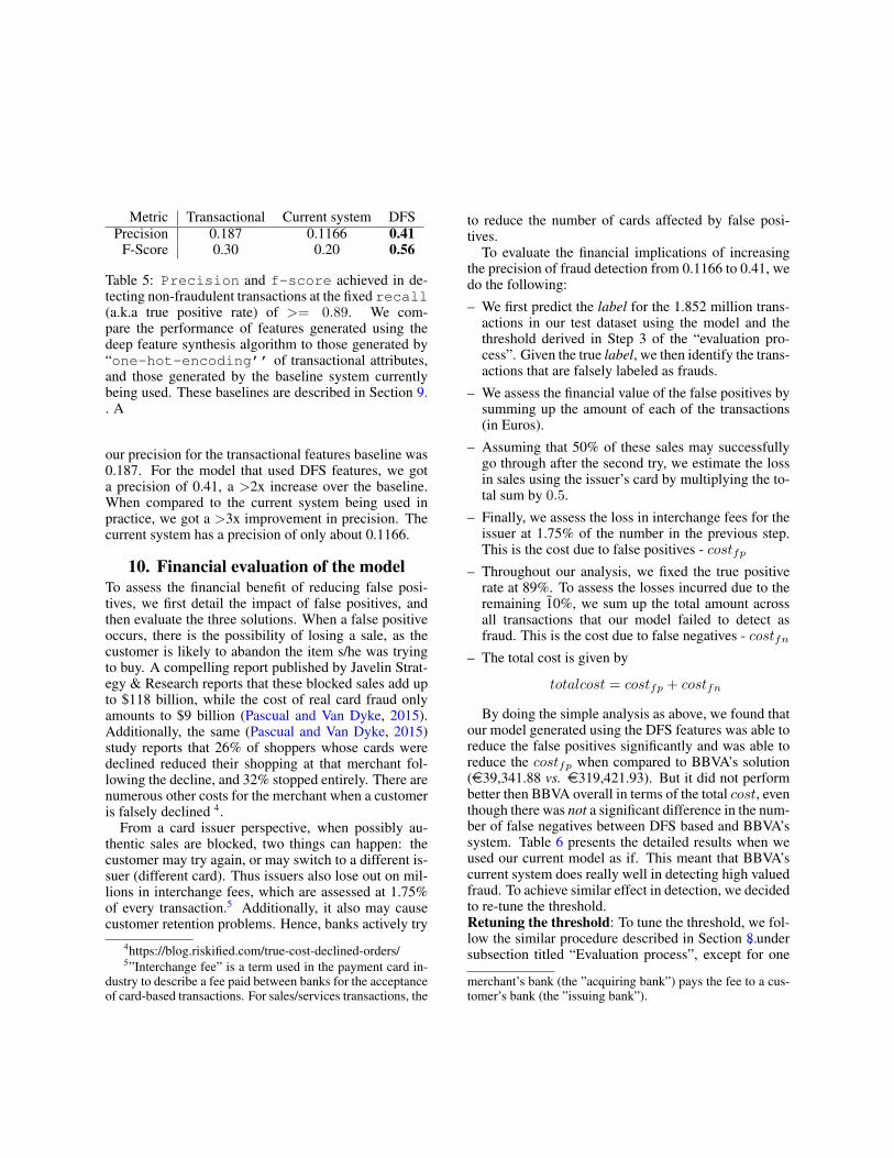
Metric Transactional Current system DFSPrecision 0.187 0.1166 0.41

F-Score 0.30 0.20 0.56

Table 5: Precision and f-score achieved in de-tecting non-fraudulent transactions at the fixed recall(a.k.a true positive rate) of >= 0.89. We com-pare the performance of features generated using thedeep feature synthesis algorithm to those generated by“one-hot-encoding’’ of transactional attributes,and those generated by the baseline system currentlybeing used. These baselines are described in Section 9.. A

our precision for the transactional features baseline was0.187. For the model that used DFS features, we gota precision of 0.41, a >2x increase over the baseline.When compared to the current system being used inpractice, we got a >3x improvement in precision. Thecurrent system has a precision of only about 0.1166.

10. Financial evaluation of the modelTo assess the financial benefit of reducing false posi-tives, we first detail the impact of false positives, andthen evaluate the three solutions. When a false positiveoccurs, there is the possibility of losing a sale, as thecustomer is likely to abandon the item s/he was tryingto buy. A compelling report published by Javelin Strat-egy & Research reports that these blocked sales add upto $118 billion, while the cost of real card fraud onlyamounts to $9 billion (Pascual and Van Dyke, 2015).Additionally, the same (Pascual and Van Dyke, 2015)study reports that 26% of shoppers whose cards weredeclined reduced their shopping at that merchant fol-lowing the decline, and 32% stopped entirely. There arenumerous other costs for the merchant when a customeris falsely declined 4.

From a card issuer perspective, when possibly au-thentic sales are blocked, two things can happen: thecustomer may try again, or may switch to a different is-suer (different card). Thus issuers also lose out on mil-lions in interchange fees, which are assessed at 1.75%of every transaction.5 Additionally, it also may causecustomer retention problems. Hence, banks actively try

4https://blog.riskified.com/true-cost-declined-orders/5”Interchange fee” is a term used in the payment card in-

dustry to describe a fee paid between banks for the acceptanceof card-based transactions. For sales/services transactions, the

to reduce the number of cards affected by false posi-tives.

To evaluate the financial implications of increasingthe precision of fraud detection from 0.1166 to 0.41, wedo the following:

– We first predict the label for the 1.852 million trans-actions in our test dataset using the model and thethreshold derived in Step 3 of the “evaluation pro-cess”. Given the true label, we then identify the trans-actions that are falsely labeled as frauds.

– We assess the financial value of the false positives bysumming up the amount of each of the transactions(in Euros).

– Assuming that 50% of these sales may successfullygo through after the second try, we estimate the lossin sales using the issuer’s card by multiplying the to-tal sum by 0.5.

– Finally, we assess the loss in interchange fees for theissuer at 1.75% of the number in the previous step.This is the cost due to false positives - costfp

– Throughout our analysis, we fixed the true positiverate at 89%. To assess the losses incurred due to theremaining 1̃0%, we sum up the total amount acrossall transactions that our model failed to detect asfraud. This is the cost due to false negatives - costfn

– The total cost is given by

totalcost = costfp + costfn

By doing the simple analysis as above, we found thatour model generated using the DFS features was able toreduce the false positives significantly and was able toreduce the costfp when compared to BBVA’s solution(e39,341.88 vs. e319,421.93). But it did not performbetter then BBVA overall in terms of the total cost, eventhough there was not a significant difference in the num-ber of false negatives between DFS based and BBVA’ssystem. Table 6 presents the detailed results when weused our current model as if. This meant that BBVA’scurrent system does really well in detecting high valuedfraud. To achieve similar effect in detection, we decidedto re-tune the threshold.Retuning the threshold: To tune the threshold, we fol-low the similar procedure described in Section 8., undersubsection titled “Evaluation process”, except for one

merchant’s bank (the ”acquiring bank”) pays the fee to a cus-tomer’s bank (the ”issuing bank”).

Method False postitives False Negatives Total Cost eNumber Cost e Number Cost e

Current system 289,124 319,421.93 4741 125,138.24 444,560Transactional features only 162,302 96,139.09 5061 818,989.95 915,129.05

DFS 53,592 39,341.88 5247 638,940.89 678,282.77

Table 6: Losses incurred due to false positives and false negatives. This table shows the results when thresholdis tuned to achieve tpr ≥ 0.89. Method: We aggregate the amount for each false positive and false negative. Falsenegatives are the frauds that are not detected by the system. We assume the issuer fully reimburses this to the client.For false positives, we assume that 50% of transactions will not happen using the card and apply a factor of 1.75%for interchange fee to calculate losses. These are estimates for the validation dataset which contained approximately1.852 million transactions.

change. In Step 2 we weight the probabilities gener-ated by the model for a transaction by multiplying theamount of the transaction to it. Thus,

P itu ← P itu × amounti (3)

We then find the threshold in this new space. Fortest data, to make a decision we do a similar transfor-mation of the probabilities predicted by a classifier fora transaction. We then apply the threshold to this newtransformed values and make a decision. This weight-ing essentially reorders the the transactions. Two trans-actions both with the same prediction probability fromthe classifier, but vastly different amounts, can have dif-ferent predictions.

Table 7 presents the results when this newthreshold is used. A few points are noteworthy:

– DFS model reduces the total cost BBVA would in-cur by atleast 190K euros. It should be noted thatthese set of transactions, 1.852 million, only repre-sent a tiny fraction of overall volume of transactionsin a year. We further intend to apply this model tolarger dataset to fully evaluate its efficacy.

– When threshold is tuned considering financial im-plications, precision drops. Compared to the pre-cision we were able to achieve previously, when wedid not tune it for high valued transactions, we getless precision (that is more false positives). In orderto save from high value fraud, our threshold gave upsome false positives.

– “Transactional features only” solution has betterprecision than existing model, but smaller finan-cial impact: After tuning the threshold to weighhigh valued transactions, the baseline that generatesfeatures only using attributes of the transaction (and

no historical information) still has a higher precisionthan the existing model. However, it performs worseon high value transaction so the overall financial im-pact is the worse than BBVA’s existing model.

– 54% reduction in the number of false positives.Compared to the current BBVA solution, DFS basedsolution cuts the number of false positives by morethan a half. Thus reduction in number of false pos-itives reduces the number of cards that are falseblocked - potentially improving customer satisfactionwith BBVA cards.

11. Real-time deployment considerationsSo far, we have shown how we can utilize complex fea-tures generated by DFS to improve predictive accuracy.Compared to the baseline and the current system, DFS-based features that utilize historical data improve theprecision by 52% while maintaining the recall at 9̃0%.

However, if the predictive model is to be useful inreal life, one important consideration is: how long doesit take to compute these features in real time, so thatthey are calculated right when the transaction happens?This requires thinking about two important aspects:

– Throughput: This is the number of predictions soughtper second, which varies according to the size ofthe client. It is not unusual for a large bank to re-quest anywhere between 10-100 predictions per sec-ond from disparate locations.

– Latency: This is the time between when a predictionis requested and when it is provided. Latency must below, on the order of milliseconds. Delays cause an-noyance for both the merchant and the end customer.

Method False postitives False Negatives Total Cost(Euros)Number Cost e Number Cost e

Current system 289,124 319,421.93 4741 125,138.24 444,560Transactional features only 214,705 190,821.51 4607 686,626.40 877,447

DFS 133,254 183,502.64 4729 71,563.75 255,066

Table 7: Losses incurred due to false positives and false negatives. This table shows the results when the thresholdis tuned to consider high valued transactions. Method:We aggregate the amount for each false positive and falsenegative. False negatives are the frauds that are not detected by the system. We assume the issuer fully reimbursesthis to the client. For false positives, we assume that 50% of transactions will not happen using the card and apply afactor of 1.75% for interchange fee to calculate losses. These are estimates for the validation dataset which containedapproximately 1.852 million transactions.

Figure 4: The process of approximating of feature values. For a transaction that happens at 1 PM on August 24, wecan extract features by aggregating from transactions up to that time point, or by aggregating up to midnight of August23, or midnight of August 20, and so on. Not shown here, these approximations implicitly impact how frequently thefeatures need to be computed. In the first case, one has to compute the features in real time, but as we move from leftto right, we go from computing on daily basis to once a month.

While throughput is a function of how many requestscan be executed in parallel as well as the time each re-quest takes (the latency), latency is strictly a functionof how much time it takes to do the necessary compu-tation, make a prediction, and communicate the predic-tion to the end-point (either the terminal or an online ordigital payment system). When compared to the pre-vious system in practice, using the complex featurescomputed with DFS adds the additional cost of com-puting features from historical data, on top of the ex-isting costs of creating transactional features and exe-cuting the model. Features that capture the aggregatestatistics can be computed in two different ways:

– Use aggregates up to the point of transaction: This

requires having infrastructure in place to query andcompute the features in near-real time, and would ne-cessitate streaming computation.

– Use aggregates computed a few time steps earlier:We call these approximate features – that is, they arethe features that were current a few time steps t ago.Thus, for a transaction happening at 1PM, August 24,we could use features generated on August 1 (24 daysold). This enables feature computation in a batchmode: we can compute features once every month,and store them in a database for every card. Whenmaking a prediction for a card, we query for the fea-tures for the corresponding card. Thus, the real-timelatency is only affected by the query time.

It is possible that using old aggregates could leadto a loss of accuracy. To see whether this would af-fect the quality of the predictions, we can simulatethis type of feature extraction during the training pro-cess. Featuretools includes an option called ap-proximate, which allows us to specify the intervals atwhich features should be extracted before they are fedinto the model. We can choose approximate = "1day", specifying that Featuretools should only aggre-gate features based on historical transactions on a dailybasis, rather than all the way up to the time of transac-tion. We can change this to approximate = "21days" or approximate = "35 days" 6. Fig-ure 4 illustrates the process of feature approximation.To test how different metrics of accuracy are effected –in this case, the precision and the f1-score – we testedfor 4 different settings: {1 day, 7 days, 21 days, and 35days}.

Using this functionality greatly affects feature com-putation time during the model training process. Byspecifying a higher number of days, we can dramati-cally reduce the computation time needed for featureextraction. This enables data scientists to test their fea-tures quickly, to see whether they are predictive of theoutcome.

Table 8 presents the results of the approximationwhen threshold has been tuned to simply achieve> 0.89 tpr. In this case, there is a loss of 0.05 in pre-cision when we calculate features every 35 days.

In Table 9 presents the precision andf1-score for different levels of approximation,when threshold is tuned taking the financial valueof the transaction into account. Surprisingly, we notethat even when we compute features once every 35days, we do not loose any precision. However, weloose approximately 67K euros in money.

Implications: This result has powerful implicationsfor our ability to deploy a highly precise predictivemodel generated using a rich set of features. It im-plies that the bank can compute the features for all cardsonce every 35 days, and still be able to achieve bet-ter accuracy then the baseline method that uses onlytransactional features. Arguably, a 0.05 increase inprecision as per Table 8 and e67K benefit as perTable 9 is worthwhile in some cases, but this should beconsidered alongside the costs it would incur to extract

6Detailed code examples using approximate are givenin Appendix

features on a daily basis. (It is also important to notethat this alternative still only requires feature extractionon a daily basis, which is much less costly than realtime.)

12. Next stepsOur next steps with the method developed in this paperare as follows:

– Evaluate financial impact of the model on all 900 mil-lion transactions.

– Measure impact of reducing false positives on cus-tomer retention.

– Test the system performance on live data in produc-tion.

AcknowledgementsBBVA authors would like to acknowledge their collab-oration with the Computer Science and Artificial intel-ligence laboratory (CSAIL) alliances program.

Open source acknowledgementsThis work would not have been possible without theopen source software Featuretools and the timespent by software engineers at Feature Labs support-ing the open source release. Likewise, acknowledge-ments are also due to open source software packages -scikit-learn, and pandas.

ReferencesBhattacharyya, S.; Jha, S.; Tharakunnel, K.; and West-

land, J. C. 2011. Data mining for credit cardfraud: A comparative study. Decision Support Sys-tems 50(3):602–613.

Brause, R.; Langsdorf, T.; and Hepp, M. 1999. Neuraldata mining for credit card fraud detection. In Toolswith Artificial Intelligence, 1999. Proceedings. 11thIEEE International Conference on, 103–106. IEEE.

Carcillo, F.; Dal Pozzolo, A.; Le Borgne, Y.-A.; Caelen,O.; Mazzer, Y.; and Bontempi, G. 2017. Scarff: ascalable framework for streaming credit card frauddetection with spark. Information fusion.

Chan, P. K.; Fan, W.; Prodromidis, A. L.; and Stolfo,S. J. 1999. Distributed data mining in credit cardfraud detection. IEEE Intelligent Systems and TheirApplications 14(6):67–74.

Metric DFS with feature approximation1 7 21 35

Precision 0.41 0.374 0.359 0.36F1-score 0.56 0.524 0.511 0.512

Total-cost 678,282.77 735,229.05 716,157.54 675,854.12

Table 8: Precision and f-score achieved in detecting non-fraudulent transactions at the fixed recall (a.k.atrue positive rate) of >= 0.89, when feature approximation is applied and threshold is tuned only to achieve atpr >= 0.89. A loss of 0.05 in precision is observed. No significant loss in financial value is noticed.

Metric DFS with feature approximation1 7 21 35

Precision 0.22 0.223 0.23 0.236F1-score 0.35 0.356 0.366 0.373

Total-cost 255,066 305,282.26 314,590.34 322,250.67

Table 9: Precision and f-score achieved in detecting non-fraudulent transactions at the fixed recall (a.k.atrue positive rate) of >= 0.89, when feature approximation is applied and threshold is tuned to weigh high valuedtransactions more. No significant loss in precision is found, but an additional cost of approximately 67K euros isincurred.

Feature primitive name DescriptionAggregation

sum sum of a numeric feature, or the number of True values in a boolean featuremean a mean value of a numeric feature ignoring

std finds the standard deviation of a numerical featurecount counts the number of non-null values

number of unique number of unique categorical variablesmode most common element in a categorical feature

average time between Maximum of absolute value of value minus previous value(diff)Transformation

weekend transform datetime feature into boolean of weekendday transform Datetime feature into the day (0 - 30) of the month, or Timedelta features into

number of days they encompass

Table 10: Numerical and Categorical feature functions

Domingos, P. 2012. A few useful things to knowabout machine learning. Communications of theACM 55(10):78–87.

Feature Labs, I. 2017. Featuretools: automated featureengineering.

Ghosh, S., and Reilly, D. L. 1994. Credit cardfraud detection with a neural-network. In SystemSciences, 1994. Proceedings of the Twenty-Seventh

Hawaii International Conference on, volume 3, 621–630. IEEE.

Kanter, J. M., and Veeramachaneni, K. 2015. Deepfeature synthesis: Towards automating data scienceendeavors. In Data Science and Advanced Analytics(DSAA), 2015. 36678 2015. IEEE International Con-ference on, 1–10. IEEE.

Panigrahi, S.; Kundu, A.; Sural, S.; and Majumdar,A. K. 2009. Credit card fraud detection: A fusion

approach using dempster–shafer theory and bayesianlearning. Information Fusion 10(4):354–363.

Pascual, Al, M.-K., and Van Dyke, A. 2015. Overcom-ing false positives: Saving the sale and the customerrelationship. In Javelin strategy and research reports.

Shen, A.; Tong, R.; and Deng, Y. 2007. Application ofclassification models on credit card fraud detection.In Service Systems and Service Management, 2007International Conference on, 1–4. IEEE.

Stolfo, S.; Fan, D. W.; Lee, W.; Prodromidis, A.; andChan, P. 1997. Credit card fraud detection usingmeta-learning: Issues and initial results. In AAAI-97Workshop on Fraud Detection and Risk Management.

Whitrow, C.; Hand, D. J.; Juszczak, P.; Weston, D.; andAdams, N. M. 2009. Transaction aggregation as astrategy for credit card fraud detection. Data Miningand Knowledge Discovery 18(1):30–55.