Chapter 10
Automated ModelSelection for MultipleRegression
Given data on a response variable Y and k predictors or binary variables
X1, X2, . . . , Xk, we wish to develop a regression model to predict Y . Assuming
that the collection of variables is measured on the correct scale, and that the
candidate list of effects includes all the important predictors or binary variables,
the most general model is
Y = β0 + β1X1 + · · · + βkXk + ε.
In most problems one or more of the effects can be eliminated from the full
model without loss of information. We want to identify the important effects,
or equivalently, eliminate the effects that are not very useful for explaining the
variation in Y .
We will study several automated non-hierarchical methods for model selec-
tion. Given a specific criterion for selecting a model, a method gives the best
model. Before applying these methods, plot Y against each predictor to see
whether transformations are needed. Although transformations of binary vari-
ables are not necessary, side-by-side boxplots of the response across the levels
of a factor give useful information on the predictive ability of the factor. If a
Prof. Erik B. Erhardt
10.1: Forward Selection 259
transformation of Xi is suggested, include the transformation along with the
original Xi in the candidate list. Note that we can transform the predictors
differently, for example, log(X1) and√X2. However, if several transformations
are suggested for the response, then one should consider doing one analysis for
each suggested response scale before deciding on the final scale.
Different criteria for selecting models lead to different “best models.” Given
a collection of candidates for the best model, we make a choice of model on the
basis of (1) a direct comparison of models, if possible (2) examination of model
adequacy (residuals, influence, etc.) (3) simplicity — all things being equal,
simpler models are preferred, and (4) scientific plausibility.
I view the various criteria as a means to generate interesting models for
further consideration. I do not take any of them literally as best.
You should recognize that automated model selection methods should not
replace scientific theory when building models! Automated methods are best
suited for exploratory analyses, in situations where the researcher has little
scientific information as a guide.
AIC/BIC were discussed in Section 3.2.1 for stepwise procedures and were
used in examples in Chapter 9. In those examples, I included the corresponding
F -tests in the ANOVA table as a criterion for dropping variables from a model.
The next few sections cover these methods in more detail, then discuss other
criteria and selections strategies, finishing with a few examples.
10.1 Forward Selection
In forward selection we add variables to the model one at a time. The steps in
the procedure are:
1. Find the variable in the candidate list with the largest correlation (ignor-
ing the sign) with Y . This variable gives a simple linear regression model
with the largest R2. Suppose this is X1. Then fit the model
Y = β0 + β1X1 + ε (10.1)
UNM, Stat 428/528 ADA2
260 Ch 10: Automated Model Selection for Multiple Regression
and test H0 : β1 = 0. If we reject H0, go to step 2. Otherwise stop and
conclude that no variables are important. A t-test can be used here, or
the equivalent ANOVA F -test.
2. Find the remaining variable which when added to model (10.1) increases
R2 the most (or equivalently decreases Residual SS the most). Suppose
this is X2. Fit the model
Y = β0 + β1X1 + β2X2 + ε (10.2)
and test H0 : β2 = 0. If we do not reject H0, stop and use model (10.1)
to predict Y . If we reject H0, replace model (10.1) with (10.2) and repeat
step 2 sequentially until no further variables are added to the model.
In forward selection we sequentially isolate the most important effect left
in the pool, and check whether it is needed in the model. If it is needed we
continue the process. Otherwise we stop.
The F -test default level for the tests on the individual effects is sometimes
set as high as α = 0.50 (SAS default). This may seem needlessly high. However,
in many problems certain variables may be important only in the presence of
other variables. If we force the forward selection to test at standard levels then
the process will never get “going” when none of the variables is important on
its own.
10.2 Backward Elimination
The backward elimination procedure (discussed earlier this semester) deletes
unimportant variables, one at a time, starting from the full model. The steps
is the procedure are:
1. Fit the full model
Y = β0 + β1X1 + · · · + βkXk + ε. (10.3)
2. Find the variable which when omitted from the full model (10.3) reduces
R2 the least, or equivalently, increases the Residual SS the least. This
Prof. Erik B. Erhardt
10.3: Stepwise Regression 261
is the variable that gives the largest p-value for testing an individual
regression coefficient H0 : βj = 0 for j > 0. Suppose this variable is Xk.
If you reject H0, stop and conclude that the full model is best. If you do
not reject H0, delete Xk from the full model, giving the new full model
Y = β0 + β1X1 + · · · + βk−1Xk−1 + ε
to replace (10.3). Repeat steps 1 and 2 sequentially until no further
variables can be deleted.
In backward elimination we isolate the least important effect left in the
model, and check whether it is important. If not, delete it and repeat the
process. Otherwise, stop. The default test level on the individual variables is
sometimes set at α = 0.10 (SAS default).
10.3 Stepwise Regression
Stepwise regression combines features of forward selection and backward elim-
ination. A deficiency of forward selection is that variables can not be omitted
from the model once they are selected. This is problematic because many vari-
ables that are initially important are not important once several other variables
are included in the model. In stepwise regression, we add variables to the model
as in forward regression, but include a backward elimination step every time a
new variable is added. That is, every time we add a variable to the model we
ask whether any of the variables added earlier can be omitted. If variables can
be omitted, they are placed back into the candidate pool for consideration at
the next step of the process. The process continues until no additional variables
can be added, and none of the variables in the model can be excluded. The
procedure can start from an empty model, a full model, or an intermediate
model, depending on the software.
The p-values used for including and excluding variables in stepwise regres-
sion are usually taken to be equal (why is this reasonable?), and sometimes set
at α = 0.15 (SAS default).
UNM, Stat 428/528 ADA2
262 Ch 10: Automated Model Selection for Multiple Regression
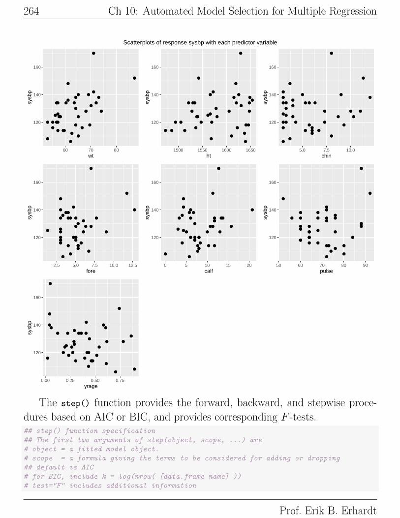
10.3.1 Example: Indian systolic blood pressure
We revisit the example first introduced in Chapter 2. Anthropologists con-
ducted a study to determine the long-term effects of an environmental change
on systolic blood pressure. They measured the blood pressure and several other
characteristics of 39 Indians who migrated from a very primitive environment
high in the Andes into the mainstream of Peruvian society at a lower altitude.
All of the Indians were males at least 21 years of age, and were born at a high
altitude.
Let us illustrate the three model selection methods to build a regression
model, using systolic blood pressure (sysbp) as the response, and seven candi-
date predictors: wt = weight in kilos; ht = height in mm; chin = chin skin fold
in mm; fore = forearm skin fold in mm; calf = calf skin fold in mm; pulse
= pulse rate-beats/min, and yrage = fraction, which is the proportion of each
individual’s lifetime spent in the new environment.
Below I generate simple summary statistics and plots. The plots do not
suggest any apparent transformations of the response or the predictors, so we
will analyze the data using the given scales.#### Example: Indian
fn.data <- "http://statacumen.com/teach/ADA2/ADA2_notes_Ch02_indian.dat"
indian <- read.table(fn.data, header=TRUE)
# Description of variables
# id = individual id
# age = age in years yrmig = years since migration
# wt = weight in kilos ht = height in mm
# chin = chin skin fold in mm fore = forearm skin fold in mm
# calf = calf skin fold in mm pulse = pulse rate-beats/min
# sysbp = systolic bp diabp = diastolic bp
# Create the "fraction of their life" variable
# yrage = years since migration divided by age
indian$yrage <- indian$yrmig / indian$age
# correlation matrix and associated p-values testing "H0: rho == 0"
library(Hmisc)
i.cor <- rcorr(as.matrix(indian[,c("sysbp", "wt", "ht", "chin"
, "fore", "calf", "pulse", "yrage")]))
# print correlations with the response to 3 significant digits
signif(i.cor$r[1, ], 3)
Prof. Erik B. Erhardt
10.3: Stepwise Regression 263
## sysbp wt ht chin fore calf pulse yrage
## 1.000 0.521 0.219 0.170 0.272 0.251 0.133 -0.276
# scatterplots
library(ggplot2)
p1 <- ggplot(indian, aes(x = wt , y = sysbp)) + geom_point(size=2)
p2 <- ggplot(indian, aes(x = ht , y = sysbp)) + geom_point(size=2)
p3 <- ggplot(indian, aes(x = chin , y = sysbp)) + geom_point(size=2)
p4 <- ggplot(indian, aes(x = fore , y = sysbp)) + geom_point(size=2)
p5 <- ggplot(indian, aes(x = calf , y = sysbp)) + geom_point(size=2)
p6 <- ggplot(indian, aes(x = pulse, y = sysbp)) + geom_point(size=2)
p7 <- ggplot(indian, aes(x = yrage, y = sysbp)) + geom_point(size=2)
library(gridExtra)
grid.arrange(grobs = list(p1, p2, p3, p4, p5, p6, p7), ncol=3
, top = "Scatterplots of response sysbp with each predictor variable")
UNM, Stat 428/528 ADA2
264 Ch 10: Automated Model Selection for Multiple Regression
●
●
●
●
●
●
●
●
●
●
●●
●
●
●
●
●●
●
●
●
●
●●
●
●
●
●
●
●
●●
●
●
●
●
●
●
●
120
140
160
60 70 80wt
sysb
p
●
●
●
●
●
●
●
●
●
●
●●
●
●
●
●
●●
●
●
●
●
●●
●
●
●
●
●
●
●●
●
●
●
●
●
●
●
120
140
160
1500 1550 1600 1650ht
sysb
p
●
●
●
●
●
●
●
●
●
●
●●
●
●
●
●
● ●
●
●
●
●
●●
●
●
●
●
●
●
●●
●
●
●
●
●
●
●
120
140
160
5.0 7.5 10.0chin
sysb
p
●
●
●
●
●
●
●
●
●
●
●●
●
●
●
●
● ●
●
●
●
●
●●
●
●
●
●
●
●
●●
●
●
●
●
●
●
●
120
140
160
2.5 5.0 7.5 10.0 12.5fore
sysb
p
●
●
●
●
●
●
●
●
●
●
●●
●
●
●
●
● ●
●
●
●
●
●●
●
●
●
●
●
●
●●
●
●
●
●
●
●
●
120
140
160
0 5 10 15 20calf
sysb
p
●
●
●
●
●
●
●
●
●
●
●●
●
●
●
●
●●
●
●
●
●
●●
●
●
●
●
●
●
●●
●
●
●
●
●
●
●
120
140
160
50 60 70 80 90pulse
sysb
p
●
●
●
●
●
●
●
●
●
●
●●
●
●
●
●
●●
●
●
●
●
●●
●
●
●
●
●
●
●●
●
●
●
●
●
●
●
120
140
160
0.00 0.25 0.50 0.75yrage
sysb
p
Scatterplots of response sysbp with each predictor variable
The step() function provides the forward, backward, and stepwise proce-
dures based on AIC or BIC, and provides corresponding F -tests.## step() function specification
## The first two arguments of step(object, scope, ...) are
# object = a fitted model object.
# scope = a formula giving the terms to be considered for adding or dropping
## default is AIC
# for BIC, include k = log(nrow( [data.frame name] ))
# test="F" includes additional information
Prof. Erik B. Erhardt
10.3: Stepwise Regression 265
# for parameter estimate tests that we're familiar with
Forward selection output The output for the forward selection method
is below. BIC is our selection criterion, though similar decisions are made as if
using F -tests.
Step 1 Variable wt =weight is entered first because it has the highest
correlation with sysbp =sys bp. The corresponding F -value is the square of
the t-statistic for testing the significance of the weight predictor in this simple
linear regression model.
Step 2 Adding yrage =fraction to the simple linear regression model
with weight as a predictor increases R2 the most, or equivalently, decreases
Residual SS (RSS) the most.
Step 3 The last table has “<none>” as the first row indicating that
the current model (no change to current model) is the best under the current
selection criterion.# start with an empty model (just the intercept 1)
lm.indian.empty <- lm(sysbp ~ 1, data = indian)
# Forward selection, BIC with F-tests
lm.indian.forward.red.BIC <- step(lm.indian.empty
, sysbp ~ wt + ht + chin + fore + calf + pulse + yrage
, direction = "forward", test = "F", k = log(nrow(indian)))
## Start: AIC=203.38
## sysbp ~ 1
##
## Df Sum of Sq RSS AIC F value Pr(>F)
## + wt 1 1775.38 4756.1 194.67 13.8117 0.0006654 ***
## <none> 6531.4 203.38
## + yrage 1 498.06 6033.4 203.95 3.0544 0.0888139 .
## + fore 1 484.22 6047.2 204.03 2.9627 0.0935587 .
## + calf 1 410.80 6120.6 204.51 2.4833 0.1235725
## + ht 1 313.58 6217.9 205.12 1.8660 0.1801796
## + chin 1 189.19 6342.2 205.89 1.1037 0.3002710
## + pulse 1 114.77 6416.7 206.35 0.6618 0.4211339
## ---
UNM, Stat 428/528 ADA2
266 Ch 10: Automated Model Selection for Multiple Regression
## Signif. codes: 0 '***' 0.001 '**' 0.01 '*' 0.05 '.' 0.1 ' ' 1
##
## Step: AIC=194.67
## sysbp ~ wt
##
## Df Sum of Sq RSS AIC F value Pr(>F)
## + yrage 1 1314.69 3441.4 185.71 13.7530 0.0006991 ***
## <none> 4756.1 194.67
## + chin 1 143.63 4612.4 197.14 1.1210 0.2967490
## + calf 1 16.67 4739.4 198.19 0.1267 0.7240063
## + pulse 1 6.11 4749.9 198.28 0.0463 0.8308792
## + ht 1 2.01 4754.0 198.31 0.0152 0.9024460
## + fore 1 1.16 4754.9 198.32 0.0088 0.9257371
## ---
## Signif. codes: 0 '***' 0.001 '**' 0.01 '*' 0.05 '.' 0.1 ' ' 1
##
## Step: AIC=185.71
## sysbp ~ wt + yrage
##
## Df Sum of Sq RSS AIC F value Pr(>F)
## <none> 3441.4 185.71
## + chin 1 197.372 3244.0 187.07 2.1295 0.1534
## + fore 1 50.548 3390.8 188.80 0.5218 0.4749
## + calf 1 30.218 3411.1 189.03 0.3101 0.5812
## + ht 1 23.738 3417.6 189.11 0.2431 0.6251
## + pulse 1 5.882 3435.5 189.31 0.0599 0.8081
summary(lm.indian.forward.red.BIC)
##
## Call:
## lm(formula = sysbp ~ wt + yrage, data = indian)
##
## Residuals:
## Min 1Q Median 3Q Max
## -18.4330 -7.3070 0.8963 5.7275 23.9819
##
## Coefficients:
## Estimate Std. Error t value Pr(>|t|)
## (Intercept) 60.8959 14.2809 4.264 0.000138 ***
## wt 1.2169 0.2337 5.207 7.97e-06 ***
## yrage -26.7672 7.2178 -3.708 0.000699 ***
## ---
## Signif. codes: 0 '***' 0.001 '**' 0.01 '*' 0.05 '.' 0.1 ' ' 1
##
## Residual standard error: 9.777 on 36 degrees of freedom
## Multiple R-squared: 0.4731,Adjusted R-squared: 0.4438
## F-statistic: 16.16 on 2 and 36 DF, p-value: 9.795e-06
Prof. Erik B. Erhardt
10.3: Stepwise Regression 267
Backward selection output The output for the backward elimination
method is below. BIC is our selection criterion, though similar decisions are
made as if using F -tests.
Step 0 The full model has 7 predictors so REG df = 7. The F -test in the
full model ANOVA table (F = 4.91 with p-value=0.0008) tests the hypothesis
that the regression coefficient for each predictor variable is zero. This test is
highly significant, indicating that one or more of the predictors is important in
the model.
The t-value column gives the t-statistic for testing the significance of the
individual predictors in the full model conditional on the other variables being
in the model.# start with a full model
lm.indian.full <- lm(sysbp ~ wt + ht + chin + fore + calf + pulse + yrage, data = indian)
summary(lm.indian.full)
##
## Call:
## lm(formula = sysbp ~ wt + ht + chin + fore + calf + pulse + yrage,
## data = indian)
##
## Residuals:
## Min 1Q Median 3Q Max
## -14.3993 -5.7916 -0.6907 6.9453 23.5771
##
## Coefficients:
## Estimate Std. Error t value Pr(>|t|)
## (Intercept) 106.45766 53.91303 1.975 0.057277 .
## wt 1.71095 0.38659 4.426 0.000111 ***
## ht -0.04533 0.03945 -1.149 0.259329
## chin -1.15725 0.84612 -1.368 0.181239
## fore -0.70183 1.34986 -0.520 0.606806
## calf 0.10357 0.61170 0.169 0.866643
## pulse 0.07485 0.19570 0.383 0.704699
## yrage -29.31810 7.86839 -3.726 0.000777 ***
## ---
## Signif. codes: 0 '***' 0.001 '**' 0.01 '*' 0.05 '.' 0.1 ' ' 1
##
## Residual standard error: 9.994 on 31 degrees of freedom
## Multiple R-squared: 0.5259,Adjusted R-squared: 0.4189
## F-statistic: 4.913 on 7 and 31 DF, p-value: 0.0008079
The least important variable in the full model, as judged by the p-value,
UNM, Stat 428/528 ADA2
268 Ch 10: Automated Model Selection for Multiple Regression
is calf =calf skin fold. This variable, upon omission, reduces R2 the least,
or equivalently, increases the Residual SS the least. So calf is the first to be
omitted from the model.
Step 1 After deleting calf , the six predictor model is fitted. At least one
of the predictors left is important, as judged by the overall F -test p-value. The
least important predictor left is pulse =pulse rate.# Backward selection, BIC with F-tests
lm.indian.backward.red.BIC <- step(lm.indian.full
, direction = "backward", test = "F", k = log(nrow(indian)))
## Start: AIC=199.91
## sysbp ~ wt + ht + chin + fore + calf + pulse + yrage
##
## Df Sum of Sq RSS AIC F value Pr(>F)
## - calf 1 2.86 3099.3 196.28 0.0287 0.8666427
## - pulse 1 14.61 3111.1 196.43 0.1463 0.7046990
## - fore 1 27.00 3123.4 196.59 0.2703 0.6068061
## - ht 1 131.88 3228.3 197.88 1.3203 0.2593289
## - chin 1 186.85 3283.3 198.53 1.8706 0.1812390
## <none> 3096.4 199.91
## - yrage 1 1386.76 4483.2 210.68 13.8835 0.0007773 ***
## - wt 1 1956.49 5052.9 215.35 19.5874 0.0001105 ***
## ---
## Signif. codes: 0 '***' 0.001 '**' 0.01 '*' 0.05 '.' 0.1 ' ' 1
##
## Step: AIC=196.28
## sysbp ~ wt + ht + chin + fore + pulse + yrage
##
## Df Sum of Sq RSS AIC F value Pr(>F)
## - pulse 1 13.34 3112.6 192.79 0.1377 0.7130185
## - fore 1 26.99 3126.3 192.96 0.2787 0.6011969
## - ht 1 129.56 3228.9 194.22 1.3377 0.2560083
## - chin 1 184.03 3283.3 194.87 1.9000 0.1776352
## <none> 3099.3 196.28
## - yrage 1 1448.00 4547.3 207.57 14.9504 0.0005087 ***
## - wt 1 1953.77 5053.1 211.69 20.1724 8.655e-05 ***
## ---
## Signif. codes: 0 '***' 0.001 '**' 0.01 '*' 0.05 '.' 0.1 ' ' 1
##
## Step: AIC=192.79
## sysbp ~ wt + ht + chin + fore + yrage
##
## Df Sum of Sq RSS AIC F value Pr(>F)
## - fore 1 17.78 3130.4 189.35 0.1885 0.667013
## - ht 1 131.12 3243.8 190.73 1.3902 0.246810
Prof. Erik B. Erhardt
10.3: Stepwise Regression 269
## - chin 1 198.30 3310.9 191.53 2.1023 0.156514
## <none> 3112.6 192.79
## - yrage 1 1450.02 4562.7 204.04 15.3730 0.000421 ***
## - wt 1 1983.51 5096.2 208.35 21.0290 6.219e-05 ***
## ---
## Signif. codes: 0 '***' 0.001 '**' 0.01 '*' 0.05 '.' 0.1 ' ' 1
##
## Step: AIC=189.35
## sysbp ~ wt + ht + chin + yrage
##
## Df Sum of Sq RSS AIC F value Pr(>F)
## - ht 1 113.57 3244.0 187.07 1.2334 0.2745301
## - chin 1 287.20 3417.6 189.11 3.1193 0.0863479 .
## <none> 3130.4 189.35
## - yrage 1 1445.52 4575.9 200.49 15.7000 0.0003607 ***
## - wt 1 2263.64 5394.1 206.90 24.5857 1.945e-05 ***
## ---
## Signif. codes: 0 '***' 0.001 '**' 0.01 '*' 0.05 '.' 0.1 ' ' 1
##
## Step: AIC=187.07
## sysbp ~ wt + chin + yrage
##
## Df Sum of Sq RSS AIC F value Pr(>F)
## - chin 1 197.37 3441.4 185.71 2.1295 0.1534065
## <none> 3244.0 187.07
## - yrage 1 1368.44 4612.4 197.14 14.7643 0.0004912 ***
## - wt 1 2515.33 5759.3 205.80 27.1384 8.512e-06 ***
## ---
## Signif. codes: 0 '***' 0.001 '**' 0.01 '*' 0.05 '.' 0.1 ' ' 1
##
## Step: AIC=185.71
## sysbp ~ wt + yrage
##
## Df Sum of Sq RSS AIC F value Pr(>F)
## <none> 3441.4 185.71
## - yrage 1 1314.7 4756.1 194.67 13.753 0.0006991 ***
## - wt 1 2592.0 6033.4 203.95 27.115 7.966e-06 ***
## ---
## Signif. codes: 0 '***' 0.001 '**' 0.01 '*' 0.05 '.' 0.1 ' ' 1
summary(lm.indian.backward.red.BIC)
##
## Call:
## lm(formula = sysbp ~ wt + yrage, data = indian)
##
## Residuals:
## Min 1Q Median 3Q Max
## -18.4330 -7.3070 0.8963 5.7275 23.9819
##
UNM, Stat 428/528 ADA2
270 Ch 10: Automated Model Selection for Multiple Regression
## Coefficients:
## Estimate Std. Error t value Pr(>|t|)
## (Intercept) 60.8959 14.2809 4.264 0.000138 ***
## wt 1.2169 0.2337 5.207 7.97e-06 ***
## yrage -26.7672 7.2178 -3.708 0.000699 ***
## ---
## Signif. codes: 0 '***' 0.001 '**' 0.01 '*' 0.05 '.' 0.1 ' ' 1
##
## Residual standard error: 9.777 on 36 degrees of freedom
## Multiple R-squared: 0.4731,Adjusted R-squared: 0.4438
## F-statistic: 16.16 on 2 and 36 DF, p-value: 9.795e-06
In the final table we are unable to drop yrage or wt from the model.
Stepwise selection output The output for the stepwise selection is given
below.
Variables are listed in the output tables in order that best improves the
AIC/BIC criterion. In the stepwise case, BIC will decrease (improve) by con-
sidering variables to drop or add (indicated in the first column by − and +).
Rather than printing a small table at each step of the step() procedure, we use
lm.XXX$anova to print a summary of the drop/add choices made.# Stepwise (both) selection, BIC with F-tests, starting with intermediate model
# (this is a purposefully chosen "opposite" model,
# from the forward and backward methods this model
# includes all the variables dropped and none kept)
lm.indian.intermediate <- lm(sysbp ~ ht + fore + calf + pulse, data = indian)
# option: trace = 0 does not print each step of the selection
lm.indian.both.red.BIC <- step(lm.indian.intermediate
, sysbp ~ wt + ht + chin + fore + calf + pulse + yrage
, direction = "both", test = "F", k = log(nrow(indian)), trace = 0)
# the anova object provides a summary of the selection steps in order
lm.indian.both.red.BIC$anova
## Step Df Deviance Resid. Df Resid. Dev AIC
## 1 NA NA 34 5651.131 212.3837
## 2 - pulse 1 2.874432 35 5654.005 208.7400
## 3 - calf 1 21.843631 36 5675.849 205.2268
## 4 + wt -1 925.198114 35 4750.651 201.9508
## 5 + yrage -1 1439.707117 34 3310.944 191.5335
## 6 - ht 1 79.870793 35 3390.815 188.7995
## 7 - fore 1 50.548149 36 3441.363 185.7131
summary(lm.indian.both.red.BIC)
##
## Call:
Prof. Erik B. Erhardt
10.4: Other Model Selection Procedures 271
## lm(formula = sysbp ~ wt + yrage, data = indian)
##
## Residuals:
## Min 1Q Median 3Q Max
## -18.4330 -7.3070 0.8963 5.7275 23.9819
##
## Coefficients:
## Estimate Std. Error t value Pr(>|t|)
## (Intercept) 60.8959 14.2809 4.264 0.000138 ***
## wt 1.2169 0.2337 5.207 7.97e-06 ***
## yrage -26.7672 7.2178 -3.708 0.000699 ***
## ---
## Signif. codes: 0 '***' 0.001 '**' 0.01 '*' 0.05 '.' 0.1 ' ' 1
##
## Residual standard error: 9.777 on 36 degrees of freedom
## Multiple R-squared: 0.4731,Adjusted R-squared: 0.4438
## F-statistic: 16.16 on 2 and 36 DF, p-value: 9.795e-06
Summary of three section methods
All three methods using BIC choose the same final model, sysbp = β0 +
β1 wt + β2 yrage. Using the AIC criterion, you will find different results.
10.4 Other Model Selection Procedures
10.4.1 R2 Criterion
R2 is the proportion of variation explained by the model over the grand mean,
and we wish to maximize this. A substantial increase in R2 is usually ob-
served when an “important” effect is added to a regression model. With the
R2 criterion, variables are added to the model until further additions give in-
consequential increases in R2. The R2 criterion is not well-defined in the sense
of producing a single best model. All other things being equal, I prefer the
simpler of two models with similar values of R2. If several models with similar
complexity have similar R2s, then there may be no good reason, at this stage
of the analysis, to prefer one over the rest.
UNM, Stat 428/528 ADA2
272 Ch 10: Automated Model Selection for Multiple Regression
10.4.2 Adjusted-R2 Criterion, maximize
The adjusted-R2 criterion gives a way to compare R2 across models with differ-
ent numbers of variables, and we want to maximize this. This eliminates some
of the difficulty with calibrating R2, which increases even when unimportant
predictors are added to a model. For a model with p variables and an intercept,
the adjusted-R2 is defined by
R̄2 = 1− n− 1
n− p− 1(1−R2),
where n is the sample size.
There are four properties of R̄2 worth mentioning:
1. R̄2 ≤ R2,
2. if two models have the same number of variables, then the model with
the larger R2 has the larger R̄2,
3. if two models have the same R2, then the model with fewer variables has
the larger adjusted-R2. Put another way, R̄2 penalizes complex models
with many variables. And
4. R̄2 can be less than zero for models that explain little of the variation in
Y .
The adjusted R2 is easier to calibrate than R2 because it tends to decrease
when unimportant variables are added to a model. The model with the maxi-
mum R̄2 is judged best by this criterion. As I noted before, I do not take any
of the criteria literally, and would also choose other models with R̄2 near the
maximum value for further consideration.
10.4.3 Mallows’ Cp Criterion, minimize
Mallows’ Cp measures the adequacy of predictions from a model, relative to
those obtained from the full model, and we want to minimize Cp. Mallows’ Cpstatistic is defined for a given model with p variables by
Cp =Residual SS
σ̂2FULL− Residual df + (p + 1)
Prof. Erik B. Erhardt
10.5: Illustration with Peru Indian data 273
where σ̂2FULL is the Residual MS from the full model with k variables X1, X2,
. . ., Xk.
If all the important effects from the candidate list are included in the model,
then the difference between the first two terms of Cp should be approximately
zero. Thus, if the model under consideration includes all the important variables
from the candidate list, then Cp should be approximately p+ 1 (the number of
variables in model plus one), or less. If important variables from the candidate
list are excluded, Cp will tend to be much greater than p + 1.
Two important properties of Cp are
1. the full model has Cp = p + 1, where p = k, and
2. if two models have the same number of variables, then the model with
the larger R2 has the smaller Cp.
Models with Cp ≈ p + 1, or less, merit further consideration. As with R2
and R̄2, I prefer simpler models that satisfy this condition. The “best” model
by this criterion has the minimum Cp.
10.5 Illustration with Peru Indian data
R2 Criterion# The leaps package provides best subsets with other selection criteria.
library(leaps)
# First, fit the full model
lm.indian.full <- lm(sysbp ~ wt + ht + chin + fore + calf + pulse + yrage, data = indian)
# Second, create the design matrix which leap uses as argument
# using model.matrix(lm.XXX) as input to leaps()
# R^2 -- for each model size, report best subset of size 5
leaps.r2 <- leaps(x = model.matrix(lm.indian.full), y = indian$sysbp
, method = 'r2'
, int = FALSE, nbest = 5, names = colnames(model.matrix(lm.indian.full)))
str(leaps.r2)
## List of 4
## $ which: logi [1:36, 1:8] FALSE TRUE FALSE FALSE FALSE TRUE ...
## ..- attr(*, "dimnames")=List of 2
UNM, Stat 428/528 ADA2
274 Ch 10: Automated Model Selection for Multiple Regression
## .. ..$ : chr [1:36] "1" "1" "1" "1" ...
## .. ..$ : chr [1:8] "(Intercept)" "wt" "ht" "chin" ...
## $ label: chr [1:8] "(Intercept)" "wt" "ht" "chin" ...
## $ size : num [1:36] 1 1 1 1 1 2 2 2 2 2 ...
## $ r2 : num [1:36] 0.99 0.99 0.989 0.976 0.845 ...
# plot model R^2 vs size of model
plot(leaps.r2$size, leaps.r2$r2, main = "R2")
# report the best model (indicate which terms are in the model)
best.model.r2 <- leaps.r2$which[which((leaps.r2$r2 == max(leaps.r2$r2))),]
# these are the variable names for the best model
names(best.model.r2)[best.model.r2]
## [1] "(Intercept)" "wt" "ht" "chin"
## [5] "fore" "calf" "pulse" "yrage"
●●●
●
●
●●●●●●●●●●
●●●●● ●●●●● ●●●●● ●●●●● ●
1 2 3 4 5 6 7 8
0.85
0.90
0.95
1.00
R2
leaps.r2$size
leap
s.r2
$r2
Adjusted-R2 Criterion, maximize# adj-R^2 -- for each model size, report best subset of size 5
leaps.adjr2 <- leaps(x = model.matrix(lm.indian.full), y = indian$sysbp
Prof. Erik B. Erhardt
10.5: Illustration with Peru Indian data 275
, method = 'adjr2'
, int = FALSE, nbest = 5, names = colnames(model.matrix(lm.indian.full)))
# plot model R^2 vs size of model
plot(leaps.adjr2$size, leaps.adjr2$adjr2, main = "Adj-R2")
# report the best model (indicate which terms are in the model)
best.model.adjr2 <- leaps.adjr2$which[which((leaps.adjr2$adjr2 == max(leaps.adjr2$adjr2))),]
# these are the variable names for the best model
names(best.model.adjr2)[best.model.adjr2]
## [1] "(Intercept)" "wt" "ht" "chin"
## [5] "yrage"
●●●
●
●
●●●●●●●●●●
●●●●● ●●●●● ●●●●● ●●●●● ●
1 2 3 4 5 6 7 8
0.85
0.90
0.95
1.00
Adj−R2
leaps.adjr2$size
leap
s.ad
jr2$a
djr2
Mallows’ Cp Criterion, minimize# Cp -- for each model size, report best subset of size 3
leaps.Cp <- leaps(x = model.matrix(lm.indian.full), y = indian$sysbp
, method = 'Cp'
, int = FALSE, nbest = 3, names = colnames(model.matrix(lm.indian.full)))
# plot model R^2 vs size of model
UNM, Stat 428/528 ADA2
276 Ch 10: Automated Model Selection for Multiple Regression
plot(leaps.Cp$size, leaps.Cp$Cp, main = "Cp")
lines(leaps.Cp$size, leaps.Cp$size) # adds the line for Cp = p
# report the best model (indicate which terms are in the model)
best.model.Cp <- leaps.Cp$which[which((leaps.Cp$Cp == min(leaps.Cp$Cp))),]
# these are the variable names for the best model
names(best.model.Cp)[best.model.Cp]
## [1] "(Intercept)" "wt" "yrage"
●
●
●
●
●
●
●
●
●
●
●●●
●●●●●
●●●
●
1 2 3 4 5 6 7 8
510
1520
2530
Cp
leaps.Cp$size
leap
s.C
p$C
p
All together The function below takes regsubsets() output and formats it
into a table.# best subset, returns results sorted by BICf.bestsubset <- function(form, dat, nbest = 5){
library(leaps)bs <- regsubsets(form, data=dat, nvmax=30, nbest=nbest, method="exhaustive");bs2 <- cbind(summary(bs)$which, (rowSums(summary(bs)$which)-1)
, summary(bs)$rss, summary(bs)$rsq, summary(bs)$adjr2, summary(bs)$cp, summary(bs)$bic);
cn <- colnames(bs2);cn[(dim(bs2)[2]-5):dim(bs2)[2]] <- c("SIZE", "rss", "r2", "adjr2", "cp", "bic");
Prof. Erik B. Erhardt
10.5: Illustration with Peru Indian data 277
colnames(bs2) <- cn;ind <- sort.int(summary(bs)$bic, index.return=TRUE); bs2 <- bs2[ind$ix,];return(bs2);
}# perform on our modeli.best <- f.bestsubset(formula(sysbp ~ wt + ht + chin + fore + calf + pulse + yrage)
, indian)op <- options(); # saving old optionsoptions(width=90) # setting command window output text width wider
i.best
## (Intercept) wt ht chin fore calf pulse yrage SIZE rss r2 adjr2## 2 1 1 0 0 0 0 0 1 2 3441.363 0.47310778 0.44383599## 3 1 1 0 1 0 0 0 1 3 3243.990 0.50332663 0.46075463## 3 1 1 0 0 1 0 0 1 3 3390.815 0.48084699 0.43634816## 3 1 1 0 0 0 1 0 1 3 3411.145 0.47773431 0.43296868## 3 1 1 1 0 0 0 0 1 3 3417.624 0.47674226 0.43189159## 3 1 1 0 0 0 0 1 1 3 3435.481 0.47400828 0.42892328## 4 1 1 1 1 0 0 0 1 4 3130.425 0.52071413 0.46432755## 4 1 1 0 1 0 0 1 1 4 3232.168 0.50513668 0.44691747## 4 1 1 0 1 1 0 0 1 4 3243.771 0.50336023 0.44493203## 4 1 1 0 1 0 1 0 1 4 3243.988 0.50332702 0.44489490## 4 1 1 1 0 1 0 0 1 4 3310.944 0.49307566 0.43343750## 5 1 1 1 1 1 0 0 1 5 3112.647 0.52343597 0.45122930## 5 1 1 1 1 0 0 1 1 5 3126.303 0.52134520 0.44882174## 5 1 1 1 1 0 1 0 1 5 3128.297 0.52103997 0.44847027## 5 1 1 0 1 1 0 1 1 5 3228.867 0.50564205 0.43073933## 5 1 1 0 1 0 1 1 1 5 3231.936 0.50517225 0.43019835## 1 1 1 0 0 0 0 0 0 1 4756.056 0.27182072 0.25214020## 6 1 1 1 1 1 0 1 1 6 3099.310 0.52547798 0.43650510## 6 1 1 1 1 1 1 0 1 6 3111.060 0.52367894 0.43436875## 6 1 1 1 1 0 1 1 1 6 3123.448 0.52178233 0.43211651## 2 1 1 0 1 0 0 0 0 2 4612.426 0.29381129 0.25457859## 6 1 1 0 1 1 1 1 1 6 3228.324 0.50572524 0.41304872## 2 1 1 0 0 0 1 0 0 2 4739.383 0.27437355 0.23406097## 2 1 1 0 0 0 0 1 0 2 4749.950 0.27275566 0.23235320## 2 1 1 1 0 0 0 0 0 2 4754.044 0.27212880 0.23169151## 6 1 1 1 0 1 1 1 1 6 3283.293 0.49730910 0.40305455## 7 1 1 1 1 1 1 1 1 7 3096.446 0.52591643 0.41886531## 1 1 0 0 0 0 0 0 1 1 6033.372 0.07625642 0.05129038## 1 1 0 0 0 1 0 0 0 1 6047.218 0.07413652 0.04911319## 1 1 0 0 0 0 1 0 0 1 6120.639 0.06289527 0.03756811## 1 1 0 1 0 0 0 0 0 1 6217.854 0.04801119 0.02228176## cp bic## 2 1.453122 -13.9989263## 3 1.477132 -12.6388375## 3 2.947060 -10.9124614## 3 3.150596 -10.6793279## 3 3.215466 -10.6053171## 3 3.394238 -10.4020763## 4 2.340175 -10.3650555## 4 3.358774 -9.1176654## 4 3.474934 -8.9779148## 4 3.477106 -8.9753065## 4 4.147436 -8.1785389## 5 4.162196 -6.9236046## 5 4.298910 -6.7528787## 5 4.318869 -6.7280169## 5 5.325728 -5.4939516## 5 5.356448 -5.4569068## 1 12.615145 -5.0439888## 6 6.028670 -3.4275113
UNM, Stat 428/528 ADA2
278 Ch 10: Automated Model Selection for Multiple Regression
## 6 6.146308 -3.2799319## 6 6.270326 -3.1249499## 2 13.177196 -2.5763538## 6 7.320289 -1.8369533## 2 14.448217 -1.5173924## 2 14.554009 -1.4305331## 2 14.595000 -1.3969306## 6 7.870614 -1.1784808## 7 8.000000 0.1999979## 1 25.402961 4.2336138## 1 25.541579 4.3230122## 1 26.276637 4.7936744## 1 27.249897 5.4082455
options(op); # reset (all) initial options
10.5.1 R2, R̄2, and Cp Summary for Peru Indian Data
Discussion of R2 results:
1. The single predictor model with the highest value of R2 has wt = weight
as a predictor: R2 = 0.272. All the other single predictor models have
R2 < 0.10.
2. The two predictor model with the highest value of R2 has weight and
yrage = fraction as predictors: R2 = 0.473. No other two predictor
model has R2 close to this.
3. All of the best three predictor models include weight and fraction as pre-
dictors. However, the increase in R2 achieved by adding a third predictor
is minimal.
4. None of the more complex models with four or more predictors provides
a significant increase in R2.
A good model using the R2 criterion has two predictors, weight and yrage.
The same conclusion is reached with R̄2, albeit the model with maximum R̄2
includes wt (weight), ht (height), chin (chin skin fold), and yrage (fraction)
as predictors.
Discussion of Cp results:
1. None of the single predictor models is adequate. Each has Cp � 1+1 = 2,
the target value.
Prof. Erik B. Erhardt
10.5: Illustration with Peru Indian data 279
2. The only adequate two predictor model has wt = weight and yrage =
fraction as predictors: Cp = 1.45 < 2 + 1 = 3. This is the minimum Cpmodel.
3. Every model with weight and fraction is adequate. Every model that
excludes either weight or fraction is inadequate: Cp � p + 1.
According to Cp, any reasonable model must include both weight and frac-
tion as predictors. Based on simplicity, I would select the model with these
two predictors as a starting point. I can always add predictors if subsequent
analysis suggests this is necessary!
10.5.2 Peru Indian Data Summary
The model selection procedures suggest three models that warrant further con-
sideration.
Predictors Methods suggesting model------------------- ------------------------------------------------------------wt, yrage BIC via stepwise, forward, and backward elimination, and C_pwt, yrage, chin AIC via stepwise and backward selectionwt, yrage, chin, ht AIC via forward selection, Adj-R2
I will give three reasons why I feel that the simpler model is preferable at
this point:
1. It was suggested by 4 of the 5 methods (ignoring R2).
2. Forward selection often chooses predictors that are not important, even
when the significance level for inclusion is reduced from the default α =
0.50 level.
3. The AIC/BIC forward and backward elimination outputs suggest that
neither chin skin fold nor height is significant at any of the standard
levels of significance used in practice. Look at the third and fourth steps
of forward selection to see this.
Using a mechanical approach, we are led to a model with weight and yrage
as predictors of systolic blood pressure. At this point we should closely examine
this model. We did this earlier this semester and found that observation 1 (the
UNM, Stat 428/528 ADA2
280 Ch 10: Automated Model Selection for Multiple Regression
individual with the largest systolic blood pressure) was fitted poorly by the
model and potentially influential.
As noted earlier this semester, model selection methods can be highly influ-
enced by outliers and influential cases. Thus, we should hold out case 1, and
re-evaluate the various procedures to see whether case 1 unduly influenced the
models selected. I will just note (not shown) that the selection methods point
to the same model when case 1 is held out. After deleting case 1, there are no
large residuals, extremely influential points, or any gross abnormalities in plots.
Both analyses suggest that the “best model” for predicting systolic blood
pressure is
sysbp = β0 + β1 wt + β2 yrage + ε.
Should case 1 be deleted? I have not fully explored this issue, but I will note
that eliminating this case does have a significant impact on the least squares
estimates of the regression coefficients, and on predicted values. What do you
think?
10.6 Example: Oxygen Uptake
An experiment was conducted to model oxygen uptake (o2up), in milligrams of
oxygen per minute, from five chemical measurements: biological oxygen demand
(bod), total Kjeldahl nitrogen (tkn), total solids (ts), total volatile solids (tvs),
which is a component of ts, and chemical oxygen demand (cod), each measured
in milligrams per liter. The data were collected on samples of dairy wastes kept
in suspension in water in a laboratory for 220 days. All observations were on
the same sample over time. We desire an equation relating o2up to the other
variables. The goal is to find variables that should be further studied with the
eventual goal of developing a prediction equation (day should not be considered
as a predictor).
We are interested in developing a regression model with o2up, or some
function of o2up, as a response. The researchers believe that the predictor
variables are more likely to be linearly related to log10(o2up) rather than o2up,
Prof. Erik B. Erhardt
10.6: Example: Oxygen Uptake 281
so log10(o2up) was included in the data set. As a first step, we should plot
o2up against the different predictors, and see whether the relationship between
o2up and the individual predictors is roughly linear. If not, we will consider
appropriate transformations of the response and/or predictors.#### Example: Oxygen uptake
fn.data <- "http://statacumen.com/teach/ADA2/ADA2_notes_Ch10_oxygen.dat"
oxygen <- read.table(fn.data, header=TRUE)
day bod tkn ts tvs cod o2up logup1 0 1125 232 7160 85.90 8905 36.00 1.562 7 920 268 8804 86.50 7388 7.90 0.903 15 835 271 8108 85.20 5348 5.60 0.754 22 1000 237 6370 83.80 8056 5.20 0.725 29 1150 192 6441 82.10 6960 2.00 0.306 37 990 202 5154 79.20 5690 2.30 0.367 44 840 184 5896 81.20 6932 1.30 0.118 58 650 200 5336 80.60 5400 1.30 0.119 65 640 180 5041 78.40 3177 0.60 −0.2210 72 583 165 5012 79.30 4461 0.70 −0.1511 80 570 151 4825 78.70 3901 1.00 0.0012 86 570 171 4391 78.00 5002 1.00 0.0013 93 510 243 4320 72.30 4665 0.80 −0.1014 100 555 147 3709 74.90 4642 0.60 −0.2215 107 460 286 3969 74.40 4840 0.40 −0.4016 122 275 198 3558 72.50 4479 0.70 −0.1517 129 510 196 4361 57.70 4200 0.60 −0.2218 151 165 210 3301 71.80 3410 0.40 −0.4019 171 244 327 2964 72.50 3360 0.30 −0.5220 220 79 334 2777 71.90 2599 0.90 −0.05
The plots showed an exponential relationship between o2up and the predic-
tors. To shorten the output, only one plot is given. An exponential relationship
can often be approximately linearized by transforming o2up to the log10(o2up)
scale suggested by the researchers. The extreme skewness in the marginal distri-
bution of o2up also gives an indication that a transformation might be needed.# scatterplots
library(ggplot2)
p1 <- ggplot(oxygen, aes(x = bod, y = o2up)) + geom_point(size=2)
p2 <- ggplot(oxygen, aes(x = tkn, y = o2up)) + geom_point(size=2)
p3 <- ggplot(oxygen, aes(x = ts , y = o2up)) + geom_point(size=2)
p4 <- ggplot(oxygen, aes(x = tvs, y = o2up)) + geom_point(size=2)
UNM, Stat 428/528 ADA2
282 Ch 10: Automated Model Selection for Multiple Regression
p5 <- ggplot(oxygen, aes(x = cod, y = o2up)) + geom_point(size=2)
library(gridExtra)
grid.arrange(grobs = list(p1, p2, p3, p4, p5), nrow=2
, top = "Scatterplots of response o2up with each predictor variable")
●
●
● ●
●●●●●●●●● ●●● ●● ●●0
10
20
30
300 600 900 1200bod
o2up
●
●
●●
● ●● ●●●● ● ●● ●●● ● ● ●0
10
20
30
150 200 250 300tkn
o2up
●
●
●●
●●●●●●●●●● ●● ●●●●0
10
20
30
4000 6000 8000ts
o2up
●
●
●●
●●●●●●●●● ●●●● ●●●0
10
20
30
60 70 80tvs
o2up
●
●
● ●
●●●●● ●● ●●●●●●●●●0
10
20
30
4000 6000 8000cod
o2up
Scatterplots of response o2up with each predictor variable
After transformation, several plots show a roughly linear relationship. A
sensible next step would be to build a regression model using log(o2up) as the
response variable.# scatterplots
library(ggplot2)
p1 <- ggplot(oxygen, aes(x = bod, y = logup)) + geom_point(size=2)
p2 <- ggplot(oxygen, aes(x = tkn, y = logup)) + geom_point(size=2)
p3 <- ggplot(oxygen, aes(x = ts , y = logup)) + geom_point(size=2)
p4 <- ggplot(oxygen, aes(x = tvs, y = logup)) + geom_point(size=2)
p5 <- ggplot(oxygen, aes(x = cod, y = logup)) + geom_point(size=2)
library(gridExtra)
grid.arrange(grobs = list(p1, p2, p3, p4, p5), nrow=2
, top = "Scatterplots of response logup with each predictor variable")
Prof. Erik B. Erhardt
10.6: Example: Oxygen Uptake 283
●
●
● ●
●●
●●
●●
●●●
●
●
●●
●
●
●
−0.5
0.0
0.5
1.0
1.5
300 600 900 1200bod
logu
p
●
●
●●
●●
● ●
●●
● ●●
●
●
●●
●
●
●
−0.5
0.0
0.5
1.0
1.5
150 200 250 300tkn
logu
p
●
●
●●
●●
●●
●●
●●●
●
●
●●
●
●
●
−0.5
0.0
0.5
1.0
1.5
4000 6000 8000ts
logu
p
●
●
●●
●●
●●
●●
●●●
●
●
●●
●
●
●
−0.5
0.0
0.5
1.0
1.5
60 70 80tvs
logu
p
●
●
● ●
●●
●●
●●
● ●●
●
●
●●
●
●
●
−0.5
0.0
0.5
1.0
1.5
4000 6000 8000cod
logu
p
Scatterplots of response logup with each predictor variable
Correlation between response and each predictor.# correlation matrix and associated p-values testing "H0: rho == 0"
library(Hmisc)
o.cor <- rcorr(as.matrix(oxygen[,c("logup", "bod", "tkn", "ts", "tvs", "cod")]))
# print correlations with the response to 3 significant digits
signif(o.cor$r[1, ], 3)
## logup bod tkn ts tvs cod
## 1.0000 0.7740 0.0906 0.8350 0.7110 0.8320
I used several of the model selection procedures to select out predictors.
The model selection criteria below point to a more careful analysis of the model
with ts and cod as predictors. This model has the minimum Cp and is selected
by the backward and stepwise procedures. Furthermore, no other model has a
substantially higher R2 or R̄2. The fit of the model will not likely be improved
substantially by adding any of the remaining three effects to this model.# perform on our model
o.best <- f.bestsubset(formula(logup ~ bod + tkn + ts + tvs + cod)
, oxygen, nbest = 3)
op <- options(); # saving old options
options(width=90) # setting command window output text width wider
o.best
## (Intercept) bod tkn ts tvs cod SIZE rss r2 adjr2 cp bic
UNM, Stat 428/528 ADA2
284 Ch 10: Automated Model Selection for Multiple Regression
## 2 1 0 0 1 0 1 2 1.0850469 0.7857080 0.7604972 1.738781 -21.82112
## 3 1 0 1 1 0 1 3 0.9871461 0.8050430 0.7684886 2.318714 -20.71660
## 3 1 0 0 1 1 1 3 1.0633521 0.7899926 0.7506163 3.424094 -19.22933
## 3 1 1 0 1 0 1 3 1.0643550 0.7897946 0.7503810 3.438642 -19.21047
## 4 1 0 1 1 1 1 4 0.9652627 0.8093649 0.7585288 4.001291 -18.16922
## 1 1 0 0 1 0 0 1 1.5369807 0.6964531 0.6795894 6.294153 -17.85292
## 2 1 0 0 0 1 1 2 1.3287305 0.7375816 0.7067088 5.273450 -17.76910
## 4 1 1 1 1 0 1 4 0.9871272 0.8050467 0.7530592 4.318440 -17.72124
## 1 1 0 0 0 0 1 1 1.5563027 0.6926371 0.6755614 6.574421 -17.60306
## 4 1 1 0 1 1 1 4 1.0388337 0.7948349 0.7401242 5.068450 -16.70015
## 2 1 0 1 0 0 1 2 1.4388035 0.7158426 0.6824124 6.870078 -16.17735
## 5 1 1 1 1 1 1 5 0.9651737 0.8093824 0.7413048 6.000000 -15.17533
## 1 1 1 0 0 0 0 1 2.0337926 0.5983349 0.5760202 13.500489 -12.25127
options(op); # reset (all) initial options
These comments must be taken with a grain of salt because we have not crit-
ically assessed the underlying assumptions (linearity, normality, independence),
nor have we considered whether the data contain influential points or outliers.lm.oxygen.final <- lm(logup ~ ts + cod, data = oxygen)
summary(lm.oxygen.final)
##
## Call:
## lm(formula = logup ~ ts + cod, data = oxygen)
##
## Residuals:
## Min 1Q Median 3Q Max
## -0.37640 -0.09238 -0.04229 0.06256 0.59827
##
## Coefficients:
## Estimate Std. Error t value Pr(>|t|)
## (Intercept) -1.370e+00 1.969e-01 -6.960 2.3e-06 ***
## ts 1.492e-04 5.489e-05 2.717 0.0146 *
## cod 1.415e-04 5.318e-05 2.661 0.0165 *
## ---
## Signif. codes: 0 '***' 0.001 '**' 0.01 '*' 0.05 '.' 0.1 ' ' 1
##
## Residual standard error: 0.2526 on 17 degrees of freedom
## Multiple R-squared: 0.7857,Adjusted R-squared: 0.7605
## F-statistic: 31.17 on 2 and 17 DF, p-value: 2.058e-06
The p-values for testing the importance of the individual predictors are
small, indicating that both predictors are important. However, two observations
(1 and 20) are poorly fitted by the model (both have ri > 2) and are individually
most influential (largest Dis). Recall that this experiment was conducted over
Prof. Erik B. Erhardt
10.6: Example: Oxygen Uptake 285
220 days, so these observations were the first and last data points collected. We
have little information about the experiment, but it is reasonable to conjecture
that the experiment may not have reached a steady state until the second time
point, and that the experiment was ended when the experimental material
dissipated. The end points of the experiment may not be typical of conditions
under which we are interested in modelling oxygen uptake. A sensible strategy
here is to delete these points and redo the entire analysis to see whether our
model changes noticeably.# plot diagnisticspar(mfrow=c(2,3))plot(lm.oxygen.final, which = c(1,4,6))
plot(oxygen$ts, lm.oxygen.final$residuals, main="Residuals vs ts")# horizontal line at zeroabline(h = 0, col = "gray75")
plot(oxygen$cod, lm.oxygen.final$residuals, main="Residuals vs cod")# horizontal line at zeroabline(h = 0, col = "gray75")
# Normality of Residualslibrary(car)qqPlot(lm.oxygen.final$residuals, las = 1, id.n = 3, main="QQ Plot")
## 1 20 7## 20 19 1
## residuals vs order of data#plot(lm.oxygen.final£residuals, main="Residuals vs Order of data")# # horizontal line at zero# abline(h = 0, col = "gray75")
UNM, Stat 428/528 ADA2
286 Ch 10: Automated Model Selection for Multiple Regression
−0.5 0.0 0.5 1.0
−0.
40.
00.
20.
40.
6
Fitted values
Res
idua
ls
●
●
●
●
●
●
●
●●
●
●
●●
●
●
●
●
●
●
●
Residuals vs Fitted
120
7
5 10 15 20
0.0
0.5
1.0
1.5
Obs. number
Coo
k's
dist
ance
Cook's distance1
20
3
0.0
0.4
0.8
1.2
Leverage hii
Coo
k's
dist
ance
●
●
●
●●
●
●
● ●● ●●● ●●
●● ● ●
●
0 0.1 0.2 0.3 0.4
0
0.5
1
1.522.53
Cook's dist vs Leverage hii (1 − hii)1
20
3
●
●
●
●
●
●
●
●●
●
●
●●
●
●
●
●
●
●
●
3000 4000 5000 6000 7000 8000 9000
−0.
4−
0.2
0.0
0.2
0.4
0.6
Residuals vs ts
oxygen$ts
lm.o
xyge
n.fin
al$r
esid
uals
●
●
●
●
●
●
●
●●
●
●
●●●
●
●
●
●
●
●
3000 4000 5000 6000 7000 8000 9000
−0.
4−
0.2
0.0
0.2
0.4
0.6
Residuals vs cod
oxygen$cod
lm.o
xyge
n.fin
al$r
esid
uals
−2 −1 0 1 2
−0.4
−0.2
0.0
0.2
0.4
0.6
QQ Plot
norm quantiles
lm.o
xyge
n.fin
al$r
esid
uals
●
●●
●
● ●● ● ● ●
●● ● ●
●
●
● ●
●
●120
7
Further, the partial residual plot for both ts and cod clearly highlightsoutlying cases 1 and 20.library(car)
avPlots(lm.oxygen.final, id.n=3)
−1000 0 1000 2000 3000
−0.
40.
00.
20.
40.
6
ts | others
logu
p |
othe
rs
●
●
●
●
●
●
●
●
●
●
●
● ●
●
●
● ●●
●
●1 20
7
3
29
−2000 0 1000 2000
−0.
20.
20.
40.
60.
8
cod | others
logu
p |
othe
rs
●
●●
●
●
●
●
●
●
●
●
●
●●
●
●
●
●●
●
1
20
73
1
9
Added−Variable Plots
Prof. Erik B. Erhardt
10.6: Example: Oxygen Uptake 287
10.6.1 Redo analysis excluding first and last obser-vations
For more completeness, we exclude the end observations and repeat the model
selection steps. Summaries from the model selection are provided.
The model selection criteria again suggest ts and cod as predictors. After
deleting observations 1 and 20 the R2 for this two predictor model jumps from
0.786 to 0.892. Also note that the LS coefficients change noticeably after these
observations are deleted.# exclude observations 1 and 20
oxygen2 <- oxygen[-c(1,20),]
Correlation between response and each predictor.# correlation matrix and associated p-values testing "H0: rho == 0"
library(Hmisc)
o.cor <- rcorr(as.matrix(oxygen2[,c("logup", "bod", "tkn", "ts", "tvs", "cod")]))
# print correlations with the response to 3 significant digits
signif(o.cor$r[1, ], 3)
## logup bod tkn ts tvs cod
## 1.000 0.813 0.116 0.921 0.717 0.806
# perform on our model
o.best <- f.bestsubset(formula(logup ~ bod + tkn + ts + tvs + cod)
, oxygen2, nbest = 3)
op <- options(); # saving old options
options(width=90) # setting command window output text width wider
o.best
## (Intercept) bod tkn ts tvs cod SIZE rss r2 adjr2 cp bic
## 2 1 0 0 1 0 1 2 0.3100332 0.8923243 0.8779675 0.1755108 -31.44424
## 3 1 0 0 1 1 1 3 0.3060781 0.8936979 0.8709189 2.0201863 -28.78498
## 3 1 1 0 1 0 1 3 0.3092614 0.8925923 0.8695764 2.1452002 -28.59874
## 3 1 0 1 1 0 1 3 0.3095352 0.8924973 0.8694610 2.1559501 -28.58281
## 1 1 0 0 1 0 0 1 0.4346881 0.8490312 0.8395956 3.0709102 -28.25153
## 2 1 1 0 1 0 0 2 0.3832495 0.8668960 0.8491488 3.0508321 -27.62812
## 2 1 0 0 1 1 0 2 0.4182487 0.8547406 0.8353727 4.4253075 -26.05510
## 4 1 1 0 1 1 1 4 0.3056566 0.8938443 0.8611810 4.0036314 -25.91941
## 4 1 0 1 1 1 1 4 0.3057789 0.8938018 0.8611255 4.0084356 -25.91221
## 4 1 1 1 1 0 1 4 0.3091249 0.8926398 0.8596058 4.1398376 -25.71632
## 5 1 1 1 1 1 1 5 0.3055641 0.8938764 0.8496583 6.0000000 -23.03449
## 1 1 1 0 0 0 0 1 0.9766926 0.6607910 0.6395904 24.3563087 -13.67975
## 1 1 0 0 0 0 1 1 1.0100759 0.6491968 0.6272716 25.6673251 -13.07480
options(op); # reset (all) initial options
Below is the model with ts and cod as predictors, after omitting the end
UNM, Stat 428/528 ADA2
288 Ch 10: Automated Model Selection for Multiple Regression
observations. Both predictors are significant at the 0.05 level. Furthermore,
there do not appear to be any extreme outliers. The QQ-plot, and the plot of
studentized residuals against predicted values do not show any extreme abnor-
malities.lm.oxygen2.final <- lm(logup ~ ts + cod, data = oxygen2)
summary(lm.oxygen2.final)
##
## Call:
## lm(formula = logup ~ ts + cod, data = oxygen2)
##
## Residuals:
## Min 1Q Median 3Q Max
## -0.24157 -0.08517 0.01004 0.10102 0.25094
##
## Coefficients:
## Estimate Std. Error t value Pr(>|t|)
## (Intercept) -1.335e+00 1.338e-01 -9.976 5.16e-08 ***
## ts 1.852e-04 3.182e-05 5.820 3.38e-05 ***
## cod 8.638e-05 3.517e-05 2.456 0.0267 *
## ---
## Signif. codes: 0 '***' 0.001 '**' 0.01 '*' 0.05 '.' 0.1 ' ' 1
##
## Residual standard error: 0.1438 on 15 degrees of freedom
## Multiple R-squared: 0.8923,Adjusted R-squared: 0.878
## F-statistic: 62.15 on 2 and 15 DF, p-value: 5.507e-08
# plot diagnisticspar(mfrow=c(2,3))plot(lm.oxygen2.final, which = c(1,4,6))
plot(oxygen2$ts, lm.oxygen2.final$residuals, main="Residuals vs ts")# horizontal line at zeroabline(h = 0, col = "gray75")
plot(oxygen2$cod, lm.oxygen2.final$residuals, main="Residuals vs cod")# horizontal line at zeroabline(h = 0, col = "gray75")
# Normality of Residualslibrary(car)qqPlot(lm.oxygen2.final$residuals, las = 1, id.n = 3, main="QQ Plot")
## 6 7 15## 18 1 2
## residuals vs order of data#plot(lm.oxygen2.final£residuals, main="Residuals vs Order of data")# # horizontal line at zero# abline(h = 0, col = "gray75")
Prof. Erik B. Erhardt
10.6: Example: Oxygen Uptake 289
−0.4 −0.2 0.0 0.2 0.4 0.6 0.8
−0.
3−
0.1
0.0
0.1
0.2
0.3
Fitted values
Res
idua
ls
●
●
●
●
●
●
●
●
●
●●
●●
●
●
●
●
●
Residuals vs Fitted
6
715
5 10 15
0.0
0.1
0.2
0.3
0.4
Obs. number
Coo
k's
dist
ance
Cook's distance4
3
7
0.0
0.1
0.2
0.3
0.4
Leverage hii
Coo
k's
dist
ance
●
●
●
●●
●
●
●
● ●●● ●
●
●
● ● ●
0 0.1 0.2 0.3 0.4
0
0.5
11.52
Cook's dist vs Leverage hii (1 − hii)4
3
7
●
●
●
●
●
●
●
●
●
●●
●●
●
●
●
●
●
3000 4000 5000 6000 7000 8000 9000
−0.
2−
0.1
0.0
0.1
0.2
Residuals vs ts
oxygen2$ts
lm.o
xyge
n2.fi
nal$
resi
dual
s
●
●
●
●
●
●
●
●
●
●●
●●
●
●
●
●
●
3000 4000 5000 6000 7000 8000
−0.
2−
0.1
0.0
0.1
0.2
Residuals vs cod
oxygen2$cod
lm.o
xyge
n2.fi
nal$
resi
dual
s
−2 −1 0 1 2
−0.2
−0.1
0.0
0.1
0.2
QQ Plot
norm quantiles
lm.o
xyge
n2.fi
nal$
resi
dual
s
●
●
●
●
●
●
●●
●
● ● ●
●●
●●
●
●6
715
library(car)
avPlots(lm.oxygen2.final, id.n=3)
−1000 0 1000 2000
−0.
40.
00.
20.
40.
6
ts | others
logu
p |
othe
rs ●
●
●
●
●
●
●
●
●
●
● ●
●
●
● ●●
●
6
715
3
2
9
−2000 −1000 0 1000 2000
−0.
20.
00.
2
cod | others
logu
p |
othe
rs
●●
●
●
●
●
●
●
●
●
●
●●
●
●
●
●
●
6
715
4
9
3
Added−Variable Plots
Let us recall that the researcher’s primary goal was to identify important
predictors of o2up. Regardless of whether we are inclined to include the end
UNM, Stat 428/528 ADA2
290 Ch 10: Automated Model Selection for Multiple Regression
observations in the analysis or not, it is reasonable to conclude that ts and cod
are useful for explaining the variation in log10(o2up). If these data were the
final experiment, I might be inclined to eliminate the end observations and use
the following equation to predict oxygen uptake:
log10(o2up) = −1.335302 + 0.000185 ts + 0.000086 cod.
Prof. Erik B. Erhardt