Automated Removal of Partial Occlusion Blur

Scott McCloskey, Michael Langer, and Kaleem Siddiqi

Centre for Intelligent Machines, McGill University{scott,langer,siddiqi}@cim.mcgill.ca

Abstract. This paper presents a novel, automated method to removepartial occlusion from a single image. In particular, we are concernedwith occlusions resulting from objects that fall on or near the lens duringexposure. For each such foreground object, we segment the completelyoccluded region using a geometric flow. We then look outward from theregion of complete occlusion at the segmentation boundary to estimatethe width of the partially occluded region. Once the area of completeocclusion and width of the partially occluded region are known, the con-tribution of the foreground object can be removed. We present experi-mental results which demonstrate the ability of this method to removepartial occlusion with minimal user interaction. The result is an imagewith improved visibility in partially occluded regions, which may conveyimportant information or simply improve the image’s aesthetics.

1 Introduction

Partial occlusions arise in natural images when an occluding object falls nearerto the lens than the plane of focus. The occluding object will be blurred in pro-portion to its distance from the plane of focus, and contributes to the exposureof pixels that also record background objects. This sort of situation can arise, forexample, when taking a photo through a small opening such as a cracked door,fence, or keyhole. If the opening is smaller than the lens aperture, some partof the door/fence will fall within the field of view, partially occluding the back-ground. This may also arise when a nearby object (such as the photographer’sfinger, or a camera strap) accidentally falls within the lens’ field of view.

Whatever its cause, the width of the partially-occluded region depends on thescene geometry and the camera settings. Primarily, the width increases with in-creasing aperture size (decreasing f -number), making partial occlusion a greaterconcern in low lighting situations that necessitate a larger aperture.

Fig. 1 (left) shows an image with partial occlusion, which has three distinctregions: complete occlusion (outside the red contour), partial occlusion (betweenthe green and red contours), and no occlusion (inside the green contour). As isthe case in this example, the completely occluded region often has little high-frequency structure because of the severe blurring of objects far from the focalplane. In addition, the region of complete occlusion can be severely underexposedwhen the camera’s settings are chosen to properly expose the background.

In [7], it was shown that it is possible to remove the partial occlusion when thelocation and width of the partially occluded region are found by a user. Because

Y. Yagi et al. (Eds.): ACCV 2007, Part I, LNCS 4843, pp. 271–281, 2007.c© Springer-Verlag Berlin Heidelberg 2007

272 S. McCloskey, M. Langer, and K. Siddiqi

Fig. 1. (Left) Example image taken through a keyhole. Of the pixels that see throughthe opening, more then 98% are partially occluded. (Right) The output of our method,with improved visibility in the partially-occluded region.

of the low contrast and arbitrary shape of the boundary between regions ofcomplete and partial occlusion, this task can be challenging, time consuming,and prone to user error. In the current paper we present an automated solution tothis vision task for severely blurred occluding objects and in doing so significantlyextend the applicability of the method in [7]. Given the input image of Fig. 1(left), the algorithm presented in this paper produces the image shown in Fig. 1(right). The user must only click on a point within each completely-occludedregion in the image, from which we find the boundary of the region of completeocclusion. Next, we find the width of the partially occluded band based on amodel of image formation under partial occlusion. We then process the imageto remove the partial occlusion, producing an output with improved visibility inthat region. Each of these steps is detailed in Sec. 4.

2 Previous Work

The most comparable work to date was presented by Favaro and Soatto [3],who describe an algorithm which reconstructs the geometry and radiance of ascene, including partially-occluded regions. While this restores the background,it requires several registered input images taken at different focal positions.

Tamaki and Suzuki [12] presented a method for the detection of completelyoccluded regions in a single image. Unlike our method, they assume that theoccluding region has high contrast with the background, and that there is noadjacent region of partial occlusion.

A more distantly related technique is presented by Levoy et al. in [5], wheresynthetic aperture imaging is used to see around occluding objects. Though this

Automated Removal of Partial Occlusion Blur 273

ability is one of the key features of their system, no effort is made to identify orremove partial occlusion in the images.

Partial occlusion also occurs in matte recovery which, while designed to ex-tract the foreground object from a natural scene, can also recover the backgroundin areas of partial occlusion. Unlike our method, matte recovery methods requireeither additional views of the same scene [8,9] or substantial user intervention[1,11]. In the latter category, users must supply a trimap, a segmentation of theimage into regions that are either definitely foreground, definitely background,or unknown/mixed. Our method is related to matte recovery, and can be viewedas a way of automatically generating, from a single image, a trimap for imageswith partial occlusion due to blurred foreground objects.

3 Background and Notation

In [7], it was shown that the well-known matting equation,

Rinput(x, y) = α(x, y)Rf + (1 − α(x, y))Rb(x, y), (1)

describes how the lens aperture combines the radiance Rb of the backgroundobject with the radiance Rf of the foreground object. The blending parameterα describes the proportion in which the two quantities combine and Rinput isthe observed radiance. Notionally, the quantity α is the fraction of the pixel’sviewing frustum that is subtended by the foreground object. Since that objectis far from the plane of focus, the frustum is a cone and α is the fraction of thatcone subtended by the occluding object.

In order to remove the contribution of the occluding object, the values of αand Rf must be found at each pixel. Given the location of the boundary betweenregions of complete and partial occlusion, the distance d between each pixel andthe nearest point on the boundary can be found. From d and the width w of thepartially occluded region, the value of α is well-approximated [7] by

α =12

− l√

1 − l2 + arcsin(l)π

, where l = min

(2,

2d

w

)− 1. (2)

This can be done if the user supplies both w and the boundary between regionscomplete and partial occlusion, as in [7]. Unfortunately, this task is time con-suming, difficult, and prone to user error. In this paper, we present an automatedsolution to this vision problem, from which we compute the values α and Rf .

4 Method

To state the vision problem more clearly, we refer to the example1 in Fig. 2. Inthis example, the partial occlusion is due to the handle of a fork directly in front1 The authors of [7] have made this image available to the public at http://www.cim.

mcgill.ca/∼scott/research.html

274 S. McCloskey, M. Langer, and K. Siddiqi

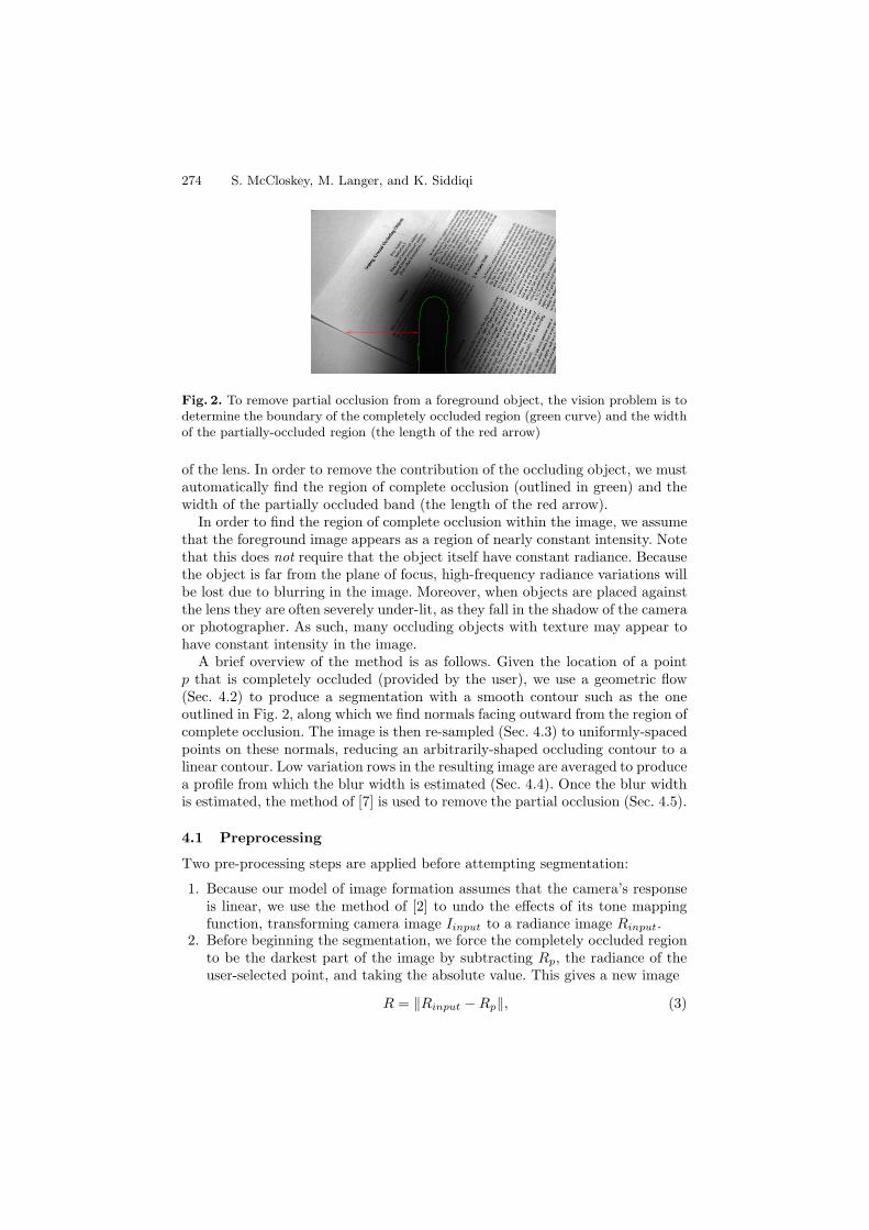
Fig. 2. To remove partial occlusion from a foreground object, the vision problem is todetermine the boundary of the completely occluded region (green curve) and the widthof the partially-occluded region (the length of the red arrow)

of the lens. In order to remove the contribution of the occluding object, we mustautomatically find the region of complete occlusion (outlined in green) and thewidth of the partially occluded band (the length of the red arrow).

In order to find the region of complete occlusion within the image, we assumethat the foreground image appears as a region of nearly constant intensity. Notethat this does not require that the object itself have constant radiance. Becausethe object is far from the plane of focus, high-frequency radiance variations willbe lost due to blurring in the image. Moreover, when objects are placed againstthe lens they are often severely under-lit, as they fall in the shadow of the cameraor photographer. As such, many occluding objects with texture may appear tohave constant intensity in the image.

A brief overview of the method is as follows. Given the location of a pointp that is completely occluded (provided by the user), we use a geometric flow(Sec. 4.2) to produce a segmentation with a smooth contour such as the oneoutlined in Fig. 2, along which we find normals facing outward from the region ofcomplete occlusion. The image is then re-sampled (Sec. 4.3) to uniformly-spacedpoints on these normals, reducing an arbitrarily-shaped occluding contour to alinear contour. Low variation rows in the resulting image are averaged to producea profile from which the blur width is estimated (Sec. 4.4). Once the blur widthis estimated, the method of [7] is used to remove the partial occlusion (Sec. 4.5).

4.1 Preprocessing

Two pre-processing steps are applied before attempting segmentation:

1. Because our model of image formation assumes that the camera’s responseis linear, we use the method of [2] to undo the effects of its tone mappingfunction, transforming camera image Iinput to a radiance image Rinput.

2. Before beginning the segmentation, we force the completely occluded regionto be the darkest part of the image by subtracting Rp, the radiance of theuser-selected point, and taking the absolute value. This gives a new image

R = ‖Rinput − Rp‖, (3)

Automated Removal of Partial Occlusion Blur 275

which is nearly zero at points in the region of complete occlusion, and higherelsewhere. As a result of this step, points on the boundary between theregions of partial and complete occlusion will have gradients ∇R that pointout of the region of complete occlusion. This property will be used to findthe boundary between the regions of complete and partial occlusion.

4.2 Foreground Segmentation

While the region of complete occlusion is assumed to have nearly constant in-tensity, segmenting this region is nontrivial due to the extremely low contrast atthe boundary between complete and partial occlusion. In order to produce goodsegmentations in spite of this difficulty, we use two cues. The first cue is that pix-els on the boundary of the region of complete occlusion have gradients of R thatpoint into the region of partial occlusion. This is assured by the pre-processing ofEq. 3, which causes the foreground object to have the lowest radiance in R. Thesecond cue is that points outside of the completely occluded region will generallyhave intensities that differ from the foreground intensity.

To exploit these two cues, we employ the flux maximizing geometric flow of[13], which evolves a 2D curve to increase the outward flux of a static vectorfield through its boundary. Our cues are embodied in the vector field

−→V = φ∇R

|∇R| , where φ = (1 + R)−2. (4)

The vector field ∇R|∇R| embodies the first cue, representing the direction of the

gradient, which is expected to align with the desired boundary as well as beorthogonal to it2. The scalar field φ, which embodies the second cue, is near 1 inthe completely-occluded region and smaller elsewhere. As noted in [6], an expo-nential form for φ can be used to produce a monotonically-decreasing functionof R, giving similar results. The curve evolution equation works out to be

Ct = div(−→V )−→N =[⟨

∇φ,∇R

|∇R|

⟩+ φκR

]−→N , (5)

where κR is the Euclidean mean curvature of the iso-intensity level set of theimage. The flow cannot leak outside the completely occluded region since byconstruction both φ and ∇φ are nearly zero there.

This curve evolution, which starts from a small circular region containing theuser-selected point, may produce a boundary that is not smooth in the presenceof noise. In order to obtain a smooth curve, from which outward normals can berobustly estimated, we apply a few iterations of the euclidean curve-shorteningflow [4]. While it is possible to include a curvature term in the flux-maximizingflow to evolve a smooth contour, we separate the terms into different flows whichare computed in sequence. Both flows are implemented using level set methods[10]; details are given in the Appendix.2 It is important to normalize the gradient of the image so that its magnitude does

not dominate the measure outside of the occluded region.

276 S. McCloskey, M. Langer, and K. Siddiqi

Fig. 3. (Left) Original image with segmentation boundary (green) and outward-facingnormals (blue) along which the image will be re-sampled. (Right) The re-sampled image(scaled), which is used to estimate the blur width.

Once the curve-shortening flow has terminated, we can recover the radianceRf of the foreground (occluding) object by simply taking the mean radiancevalue within the segmented (completely occluded) region. Note that we use thisinstead of Rp, the radiance of the user-selected point, as there may be somelow-frequency intensity variation within the region of complete occlusion.

4.3 Boundary Rectification and Profile Generation

One of the difficulties in measuring the blur width is that the boundary of thecompletely occluded region can have an arbitrary shape. In order to handle this,we re-sample the image R along outward-facing normals to the segmentationboundary, reducing the shape of the occluding contour to a line along the leftedge of a re-sampled image Rl. The number of rows in Rl is determined by thenumber of points on the segmentation boundary, and pixels in the same rowof Rl come from points on the same outward-facing normal. Pixels in the samecolumn come from points the same distance from the segmentation boundary ondifferent normals and thus, recalling Eq. 2, have the same α value. The number ofcolumns in the image depends on the distance from the segmentation boundaryto the edge of the input image. We choose this quantity to be the largest valuesuch that 80% of the normals remain within the image frame and do not re-enterthe completely-occluded region (this exact quantity is arbitrary and the methodis not sensitive to variations in this choice). Fig. 3 shows outward-facing surfacenormals from the contour in Fig. 2, along with the re-sampled image.

The task of measuring the width of the partially occluded region is also com-plicated by the generality of the background intensity. In the worst case, itis impossible (for human observers or our algorithm) to estimate the width ifthe background has an intensity gradient in the opposite direction of the in-tensity gradient due to partial occlusion. The measurement is straightforwardif the background object had constant intensity, though this assumption is toostrong. Given that the blurred region is a horizontal feature in the re-sampledimage, we average rows of Rl in order to smooth out high-frequency background

Automated Removal of Partial Occlusion Blur 277

0 20 40 60 80 100 120 140 1600

0.2

0.4

0.6

0.8

1

1.2

1.4

1.6

1.8

2

x

P(x

)

20 40 60 80 100 120 140 1600

0.005

0.01

0.015

0.02

0.025

0.03

w′

Fitt

ing

Err

or

Fig. 4. [Left] Profile generated from the re-sampled image in Fig. 3 (black curve). Modelprofile P 50

m with relatively high error (red curve). Model profile P 141m with minimum

error (green curve). [Right] Fitting error as a function of w′.

texture. While we do not assume a uniform background, we have found it usefulto eliminate rows with relatively more high-frequency structure before averaging.In particular, for each row of Rl we compute the sum of its absolute horizontalderivatives ∑

x

‖Rl(x + 1, y) − Rl(x − 1, y)‖. (6)

Rows with an activity measure in the top 70% are discarded, and the remainingrows are averaged to generate the one dimensional blur profile P .

4.4 Blur Width Estimation

Given a 1D blur profile P , like the one shown in Fig. 4 (black curve), we mustestimate the width w of the partially occluded region. We do this by first express-ing P in terms of α. Recalling Eq. 3 and the fact that Rf ≈ Rp, we rearrangeEq. 1 to get

Rl(x, y) = (1 − α(x, y))‖Rlb(x, y) − Rf‖, (7)

where Rlb is the radiance of the background object defined on the same lattice

as the re-sampled image. The profile P (x) is the average of many radiances frompixels with the same α value, so

P (x) = (1 − α(x))‖Rlb(x) − Rf‖, (8)

where Rlb(x) is the average radiance of background points a fixed distance from

the segmentation boundary (which fall in a column of the re-sampled image).As we have removed rows with significant high-frequency structure and averagedthe rows of the re-sampled image, we assume that the values Rl

b(x) are relativelyconstant over the partially-occluded band, and thus

P (x) = (1 − α(x))‖Rlb − Rf‖. (9)

Based on this, the blur width w is taken to be the value that minimizes theaverage fitting error between the measured profile P and model profiles. The

278 S. McCloskey, M. Langer, and K. Siddiqi

model profile Pw′

m for a given width w′ is constructed by first generating a linearramp l and then transforming these values into α values by Eq. 2.

An example is shown in Fig. 4, where the green curve shows the model profilefor which the error is minimized with respect to the measured profile (blackcurve), and the red curve shows another model profile which has higher error.A plot of the error as a function of w′ is shown in figure 4. We see that it has awell-defined global minimum, which is at w = 141 pixels.

4.5 Blur Removal

Once the segmentation boundary and the width w of the partially-occludedregion have been determined, the value of α can be found using Eq. 2. In orderto compute α at each pixel, we must find its distance to the nearest point onthe segmentation boundary. We employ the fast marching method of [10].

Recall that the radiance Rf of the foreground object was found previously, sowe can recover the radiance of the background at pixel (x, y) according to

Rb(x, y) =Rinput(x, y) − α(x, y)Rf

1 − α(x, y). (10)

Finally, the processed image Rb is tone-mapped to produce the output image.This tone-mapping is simply the inverse of what was done in section 4.1.

5 Experimental Results

Fig. 5 shows the processed result from the example image in Fig. 2. The user-selected point was near the center of the completely occluded region though, inour experience, the segmentation is insensitive to the location of the initial point.We also show enlargements of a region near the occluding contour to illustratethe details that become clearer after processing. Near the contour, as α → 1,noise becomes an issue. This is because we are amplifying a small part of theinput signal, namely the part that was contributed by the background.

Fig. 5. (Left) Result for the image shown in Fig. 2. (Center) Enlargement of processedresult. (Right) Enlargement of the corresponding region in the input image.

Automated Removal of Partial Occlusion Blur 279

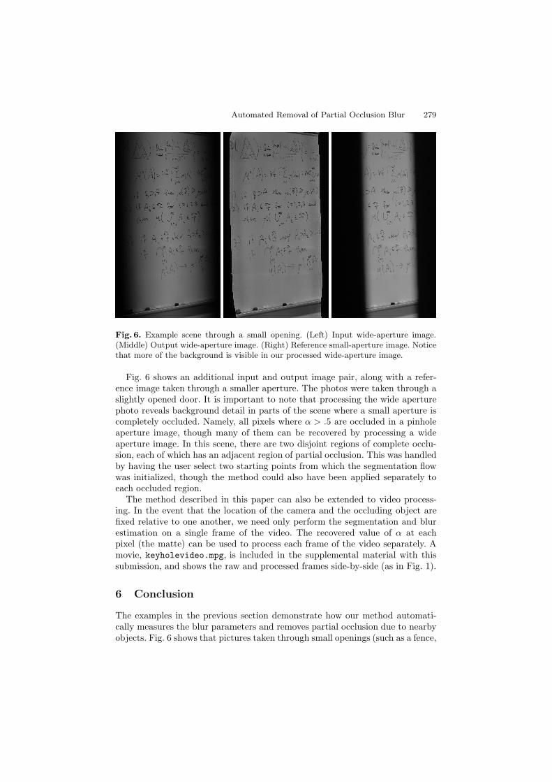
Fig. 6. Example scene through a small opening. (Left) Input wide-aperture image.(Middle) Output wide-aperture image. (Right) Reference small-aperture image. Noticethat more of the background is visible in our processed wide-aperture image.

Fig. 6 shows an additional input and output image pair, along with a refer-ence image taken through a smaller aperture. The photos were taken through aslightly opened door. It is important to note that processing the wide aperturephoto reveals background detail in parts of the scene where a small aperture iscompletely occluded. Namely, all pixels where α > .5 are occluded in a pinholeaperture image, though many of them can be recovered by processing a wideaperture image. In this scene, there are two disjoint regions of complete occlu-sion, each of which has an adjacent region of partial occlusion. This was handledby having the user select two starting points from which the segmentation flowwas initialized, though the method could also have been applied separately toeach occluded region.

The method described in this paper can also be extended to video process-ing. In the event that the location of the camera and the occluding object arefixed relative to one another, we need only perform the segmentation and blurestimation on a single frame of the video. The recovered value of α at eachpixel (the matte) can be used to process each frame of the video separately. Amovie, keyholevideo.mpg, is included in the supplemental material with thissubmission, and shows the raw and processed frames side-by-side (as in Fig. 1).

6 Conclusion

The examples in the previous section demonstrate how our method automati-cally measures the blur parameters and removes partial occlusion due to nearbyobjects. Fig. 6 shows that pictures taken through small openings (such as a fence,

280 S. McCloskey, M. Langer, and K. Siddiqi

keyhole, or slightly opened door) can be processed to improve visibility. In thisand the case of the text image shown in Fig. 5, this method reveals importantimage information that was previously difficult to see.

The automated nature of this method makes the recovery of partially-occludedscene content accessible to the average computer user. Users need only specify asingle point in each completely occluded region, and the execution time of 10-20seconds is likely acceptable. Given such a tool, users could significantly improvethe quality of images with partial occlusions.

In order to automate the recovery of the necessary parameters, we have as-sumed that the combination of blurring and under-exposure produces a fore-ground region with nearly constant intensity. Methods that allow us to relaxthis assumption are the focus of ongoing future work, and must address signifi-cant additional complexity in each of the segmentation, blur width estimation,and blur removal steps.

References

1. Chuang, Y., Curless, B., Salesin, D.H., Szeliski, R.: A Bayesian Approach to DigitalMatting. In: CVPR 2001, pp. 264–271 (2001)

2. Debevec, P., Malik, J.: Recovering High Dynamic Range Radiance Maps fromPhotographs. In: SIGGRAPH 1997, pp. 369–378 (1997)

3. Favaro, P., Soatto, S.: Seeing Beyond Occlusions (and other marvels of a finite lensaperture). In: CVPR 2003, pp. 579–586 (2003)

4. Grayson, M.: The Heat Equation Shrinks Embedded Plane Curves to RoundPoints. Journal of Differential Geometry 26, 285–314 (1987)

5. Levoy, M., Chen, B., Vaish, V., Horowitz, M., McDowall, I., Bolas, M.: SyntheticAperture Confocal Imaging. In: SIGGRAPH 2004, pp. 825–834 (2004)

6. Perona, P., Malik, J.: Scale-Space and Edge Detection using Anisotropic Diffusion.IEEE Trans. on Patt. Anal. and Mach. Intell. 12(7), 629–639 (1990)

7. McCloskey, S., Langer, M., Siddiqi, K.: Seeing Around Occluding Objects. In: Proc.of the Int. Conf. on Patt. Recog. vol. 1, pp. 963–966 (2006)

8. McGuire, M., Matusik, W., Pfister, H., Hughes, J.F., Durand, F.: Defocus VideoMatting. ACM Trans. Graph. 24(3) (2005)

9. Reinhard, E., Khan, E.A.: Depth-of-field-based Alpha-matte Extraction. In: Proc.2nd Symp. on Applied Perception in Graphics and Visualization 2005, pp. 95–102(2005)

10. Sethian, J.A.: Level Set Methods and Fast Marching Methods. Cambridge Univer-sity Press, Cambridge (1999)

11. Sun, J., Jia, J., Tang, C., Shum, H.: Poisson Matting. ACM Trans. Graph. 23(3)(2004)

12. Tamaki, T., Suzuki, H.: String-like Occluding Region Extraction for BackgroundRestoration. In: Proc. of the Int. Conf. on Patt. Recog. vol. 3, pp. 615–618 (2006)

13. Vasilevskiy, A., Siddiqi, K.: Flux Maximizing Geometric Flows. IEEE Trans. onPatt. Anal. and Mach. Intell. 24(12), 1565–1578 (2002)

Appendix: Implementation Details

For the experiments shown here, we down-sample the original 6MP images to334 by 502 pixels for segmentation and blur width estimation. Blur removal is

Automated Removal of Partial Occlusion Blur 281

performed on the original 6MP images. Based on this, blur estimation and imageprocessing takes approximately 10 seconds (on a 3 GHz Pentium IV) to producethe output in Fig. 5. Other images take more or less time, depending on the sizeof the completely-occluded region. Readers should note that some of the codeused in this implementation was written in Matlab, implying that the executiontime could be further reduced in future versions.

As outlined in section 4.2, we initially use a flux-maximizing flow to performthe segmentation, followed by a euclidean curve-shortening flow to produce asmooth contour. For the flux-maximizing flow, we evolve the level function withspeed Δt = 0.1. This parameter was chosen to ensure stability for our 6MPimages; in general it depends on image size. The evolution’s running time de-pends on the size of the foreground region. The curve evolution is terminatedif it fails to increase the segmented area by 0.01% over 10 iterations. As theflux-maximizing flow uses an image-based speed term, we use a narrow-bandimplementation [10] with a bandwidth of 10 pixels.