Page 1
Automated Stock Trading and Portfolio
Optimization Using XCS Trader and Technical
Analysis
Anil Chauhan
[email protected]
Master of Science
Artificial Intelligence
School of Informatics
University of Edinburgh
2008
Page 2
AbstractFinancial market is highly dynamic system for which finding underlying price pattern is highly
complex. We have extended the previous work done on automatic stock trading using extended
classifier system (XCS) by implementing Q (1) and Q (λ) Reinforcement Learning algorithm.
We developed 14 XCS agents using different technical indicators like Moving
averages,RSI,CMF,SAR,ADX etc. We showed that by modeling financial prediction as single
step reinforcement learning problem and using the concept of delayed reward for checking
correctness of action taken, all the benchmarks strategies like buy and hold, 'keeping money in
bank' etc could be beaten. We have also shown that stock price movement is co-related with
other day price movement and reformulated the financial forecasting as a multi step process.
We introduced the concept of passive set and found that multi step problem formulation gives
best results. Q learning gave 18% better performance than single step reward only RL. Finally
we build a portfolio management and optimization system which learns online and does
monthly or quarterly rebalancing using the best trader to trade. The results showed that
reacting to the market dynamics doesn’t necessarily give us the best result. We showed that
such a system give us average performance between the best trader and the worst trader. We
also employed different trading strategies like “using more than 1 best agent” and “mean
reversal strategy” to do portfolio optimization.
ii
Page 3
AcknowledgementsI would like to thank my supervisor Sonia Schulenburg for introducing me to the world of
Finance and Classifier Systems and for giving constant feed back on my project. I would also
like to thank Abu ul Hassan for sharing previous version of XCS java code with me. Many
thanks to my friend Santosh for reviewing my initial draft of thesis and sharing ideas on the
same.
iii
Page 4
Declaration
I declare that this thesis was composed by me, that the work contained herein is my own except
where explicitly stated otherwise in the text, and that thesis work has not been submitted for
any other degree or professional qualification except as specified.
(Anil Chauhan
[email protected] )
iv
Page 5
Table of Contents
1 Introduction..............................................................................................................................1
1.1 Introduction and Purpose....................................................................................................1
1.2 Motivation...........................................................................................................................2
1.3 Objective ............................................................................................................................3
1.4 Outline................................................................................................................................4
2 Background & Related Work.................................................................................................5
2.1 Background.........................................................................................................................5
2.1.1 Market Efficiency........................................................................................................5
2.1.1.1 Version of Efficient Market Hypothesis (EMH)..................................................52.1.2 Technical Analysis.......................................................................................................6
2.1.3 The Portfolio:..............................................................................................................6
2.1.3.1 Why do we need Portfolio?..................................................................................72.1.3.2 Portfolio Management:.........................................................................................7
2.2 Related Work......................................................................................................................7
2.2.1 Machine Learning in Finance and Portfolio Management.........................................8
2.3 XCS Introduction from Stock Trading Perspective..........................................................10
2.3.1 XCS Input and Output...............................................................................................11
2.3.2 XCS Frame Work [15]..............................................................................................12
2.3.3 XCS Learning Cycle..................................................................................................13
2.3.3.1 Updating XCS Parameters..................................................................................152.3.3.2 Genetic Algorithm role and rule evolution[15]..................................................15
2.3.4 Deviation from other LCS based Systems.................................................................16
2.3.5 Mind of XCS System..................................................................................................17
3 Implementation .....................................................................................................................18
3.1 Technical Analysis Usage in XCS....................................................................................18
3.1.1 Description of individual technical Indicators..........................................................19
3.1.2 Combining different technical indicators and working mechanism of different
Agents.................................................................................................................................24
v
Page 6
3.1.2.1 Composition of 14 Agents:.................................................................................253.1.3 Advantage and “Scope of Improvement” of current approach................................26
3.2 Improving the learning of eXtended Classifier System....................................................27
3.2.1 Classifiers in multi step Reinforcement learning problems......................................28
3.2.2 Implementing Q learning in Classifier......................................................................30
3.2.3 Eligibility trace and Watkins's Q(λ) .........................................................................30
4 Experimentation.....................................................................................................................32
4.1 FTSE data and Stability of the XCS System....................................................................32
4.1.1 FTSE Data.................................................................................................................32
4.1.2 Stability of the XCS System.......................................................................................32
4.2 Comparative Study of the 3 different Algorithm..............................................................34
4.2.1 Setting the parameters for the experiments...............................................................34
4.2.1.1 Setting Initial Exploration Rate..........................................................................354.2.1.2 Setting discount rate (gamma)............................................................................364.2.1.3 Setting Trace Decay Parameter...........................................................................37
4.3 Experimental Results for 3 learning Algorithm................................................................37
4.3.1 Observations:............................................................................................................39
4.4 Fault in the previous Reward giving strategy...................................................................40
4.4.1 Experiments with improved delayed reward Strategy...............................................40
4.4.1.1 Setting Initial Exploration Rate..........................................................................414.4.1.2 Setting Discount Rate (gamma)..........................................................................424.4.1.3 Setting Trace Decay (λ)......................................................................................42
4.4.2 Results with new delayed reward strategy................................................................43
4.4.2.1 Observations:......................................................................................................454.4.3 Experimental Results for all 3 learning algorithm with new delayed reward strategy
............................................................................................................................................48
4.4.3.1 Observations.......................................................................................................514.4.4 Fault in Q (1) learning ............................................................................................51
4.4.5 Experimentation with passive Set..............................................................................52
4.4.5.1 Finding optimum parameters..............................................................................524.4.5.2 Observations for Passive set...............................................................................55
5 Implementation & Experimentation-Portfolio Optimization............................................58
5.1 Implementation.................................................................................................................59
vi
Page 7
5.2 Portfolio Performance:......................................................................................................60
5.3 Results...............................................................................................................................61
Portfolio Management Results –.......................................................................................62
5.3.1.1 Observations: Portfolio Management results......................................................635.3.1.2 Analysis and Comments on Portfolio Management System..............................63
5.3.2 Change of Portfolio construction Strategy................................................................64
5.3.2.1 Results of Portfolio Management using more than 1 Agent...............................655.4 Experimentation with Portfolio Management taking few best companies in the Portfolio
................................................................................................................................................65
5.4.1 Steps Followed..........................................................................................................66
5.4.2 Results.......................................................................................................................66
5.4.3 Observation:..............................................................................................................66
5.4.4 Experimentation with Mean Reversal Strategy.........................................................67
5.4.4.1 Results.................................................................................................................675.4.4.2 Observations.......................................................................................................68
6 Conclusion & Future Work..................................................................................................69
6.1 Conclusion .......................................................................................................................69
6.2 Future Work......................................................................................................................71
Bibliography..............................................................................................................................72
Appendix....................................................................................................................................76
vii
Page 8
List of Figures
Figure1 XCS Frame Work [15]...............................................................................................13
Figure 2: Voting Strategy [19].................................................................................................17
Figure3: Q-learning: An off-policy TD control algorithm. [14]...........................................29
Figure4:Back ward view of eligibility trace [14]....................................................................30
Figure5: Tabular version of Watkins's Q (λ) algorithm. [14]...............................................31
Figure6: Mean Performance of 5 companies for different number of runs........................34
Figure7: DSGI Price Chart .....................................................................................................46
Figure8: DSGI, Wealth Chart of agents with old reward strategy......................................46
Figure9: DSGI, Agent’s performance with new delayed reward giving strategy...............47
Figure10: LAND, Price Chart.................................................................................................47
Figure11: LAND, Meta Agents wealth chart with old reward strategy..............................48
Figure12: LAND, Meta Agents wealth chart with new delayed reward strategy...............48
Figure13: Portfolio Management Results...............................................................................62
Figure14: Portfolio management using either best 5 or best 10 or best 20 companies......66
Figure15: Portfolio Management System using trend reversal strategy.............................67
Figure16: Comparison mean reversal strategy with normal strategy.................................68
viii
Page 9
List of Tables
Table1. Composition of different Agents................................................................................26
Table2: Details of 10 FTSE 100 Companies...........................................................................32
Table3: Experimental results for 100 run on 5 FTSE100 companies..................................33
Table4: Setting Exploration rate.............................................................................................35
Table5: Combined Results for Different exploration rate....................................................36
Table6: Setting discount rate...................................................................................................36
Table7: Setting trace decay parameter...................................................................................37
Table8: Experimental Results for 3 learning methodology..................................................39
Table9: Setting Exploration Rate............................................................................................41
Table10: Setting discount rate.................................................................................................42
Table11: Setting trace decay....................................................................................................42
Table12: Comparative results for 90 FTSE 100 companies with delayed reward strategy
for single step reward only RL................................................................................................45
Table13: Results of 90 FTSE100 Companies for different RL with new delayed reward
strategy.......................................................................................................................................50
Table 14: Comparative Results for FTSE 100 companies using Passive Set......................54
Table15: Comparison with Only active set and with additional passive set approach......55
Table16: Combined Results single step RL without Passive set and multi step Q Learning
with passive set..........................................................................................................................57
Table17: Portfolio Optimization using single best Agent....................................................61
Table18: Monthly Portfolio management Using Best 3 agents.............................................64
Table19: Monthly Portfolio Rebalancing using different Number of Best Agents............65
Table 20: Portfolio Management System with quarterly re-balancing taking best 5
companies..................................................................................................................................65
Page 11
Chapter 1
1 Introduction
1.1 Introduction and PurposeAdvances in modern machine learning such as evolutionary computation have
enabled us not only to analyze data more efficiently, but also to understand any
underlying patterns present in the financial market. This effective exploitation of new
computation methods will help organizations to make better informed decisions which
will further improve their competitive edge [5]. Many different approaches like Neural
Networks (NN), Genetic Algorithms (GA) have been widely applied to predict the
financial market. However, for some of these systems the input data might not be as
rich in information content as technical indicators such as various types of moving
averages, break out rules, maximum and minimum prices in the preceding days or
fundamental indicators such as dividends, interest rates and money supply. More
recently, the academic world has shown some promise in the area of learning classifier
systems (rule based models) by Overcoming some of the most common drawbacks
neural models present to practitioners, such as the lack of explanatory power, high
variance in results and the need to continually retrain the nets when performance starts
to decrease. In addition, very few models have addressed the integration of more than
one learning paradigm within a single platform.
In this project, first we will try to improve the learning of the classifier system
by incorporating different Reinforcement learning algorithm. In all the previous
version of eXtended Classifier Systems (XCS), financial forecasting was solely
considered to be a single step Reinforcement Learning problem. However, we believe
price movement is not completely erratic and prices do follows patterns of ups and
downs. Price of any day affects the coming day prices and is in some way co-related.
Due to this we will try to model financial forecasting as a multi step process and
1
Page 12
implement Q (1) and Q (λ) Reinforcement Learning algorithm. Secondly, we will
investigate the methods of portfolio construction and portfolio optimization. This will
be achieved by using a system which evolves technical trading agents, each learning to
trade stocks by modeling groups of traders using a variety of sets of technical
indicators. For portfolio construction, the main task will be to build a portfolio
management system attached to XCS which picks the best agents that can give the
maximum benefit in the long run. For simplicity, the equity market will be the prime
focus for this investigation, although (if time permits), tests could be extended to
foreign exchange to address scalability of the approach.
1.2 MotivationThe financial market is a highly dynamic system which depends on multiple
factors such as bank interest rates, company base strength and everyday changing
news. The motivation behind this project is to develop learning systems that can learn
in an online fashion and cope with rapidly changing financial market environment.
The main idea is to develop set of robust agents which uses Technical Analysis
information and different Reinforcement Learning Algorithm to do automatic stock
trading using eXtended Classifier System (XCS). They should be robust in the sense
that they should be able to trade profitably (beat different benchmark strategies) on all
FTSE 100 stocks. Finally we wish to build a portfolio optimization system which will
interact with this modified eXtended Classifier System (XCS) and harnesses the
strength of best agents and use different strategies like “taking best companies in the
portfolio”,”mean reversal strategies” etc to do monthly or quarterly portfolio
rebalancing.
2
Page 13
1.3 Objective The project has been subdivided into following sub tasks -:
1) Optimize the problem formulation for XCS: The agents present in current
system converts the information given by the technical indicators into Input
(Binary String) for the XCS. The XCS System further tries to learn the
optimum decision it should take when faced with a particular combination of
binary bits. The better we define the problem (i.e. combine the technical
indicator information) for the XCS, the better it will learn the underlying price
pattern and more robust and reliable decisions (buy, sell or hold) we expect it
to give. The aim is to develop such robust agents.
2) Formulate automatic stock trading and financial forecasting as a multi step
problem instead of single step problem by implementing Q learning and Q (λ)
learning algorithm.
3) Experiment with reward mechanism of XCS reinforcement learning portion to
see if the delayed reward feedback is better than currently employed immediate
reward feedback.
4) Explore the possibility of either giving negative reward to the agents for taking
any incorrect action or creating and rewarding passive set for the incorrect
decision taken by an agent.
5) Build a Portfolio Management System attached to the current XCS System.
The portfolio management system will be responsible for -:
a) Portfolio construction using different trading strategies like "utilizing
combinations of best agents instead of a single agent", "mean reversal
strategies" etc.
b) Optimize the portfolio by pro-active monthly, quarterly or yearly
rebalancing.
6) Compare the performance of the trading agents against benchmark agents like
buy and hold, bank etc.
3
Page 14
1.4 OutlineThe rest of this thesis is organized as follows:
Chapter 2 gives the background information on the subject and briefs the
readers about the current state of the art in “Financial forecasting domain”.
Chapter 3 talks about how we have implemented different agents and learning
algorithm as proposed in this thesis. It also talks about what errors we found
during implementation and how we changed our approach to tackle different
problems.
Chapter 4 presents the experimental results obtain after implementing different
Learning algorithm and our critical analysis of the results.
Chapter 5 presents the implementation and experimental results for portfolio
construction and optimization system and critical analysis of the same.
4
Page 15
Chapter 2
2 Background & Related Work
2.1 Background
2.1.1 Market Efficiency
Maurice Kendall in his random walk experiment (1953) [16] found that the
stock prices are completely random and has no relation to the past performance. The
unpredictable price movement seems to confirm the irrationality of the market.
However, on deeper analysis it became apparent that random price movement
indicates a well functioning or efficient market and not an irrational one [17]. In its
most basic form Efficient Market Hypothesis says that markets are information
efficient i.e. all the available information that could be used for profit making
quickly gets absorbed in the stock prices and the prices may increase or decrease only
in response to new unavailable and unpredictable information.
2.1.1.1 Version of Efficient Market Hypothesis (EMH)
There are 3 forms of EMH, which differs in what “all available information” is
composed of.
1) Weak Form hypothesis states that stock prices already reflect all the market
trading information like past price, volume movement etc. It means that if any
form of past price or volume data movement could be used be generate reliable
trading signal then all investors would have used them by now making the
information fruitless[17]. It suggests that any form of Technical analysis is
useless.
2) Semi strong form hypothesis states that any publicly available information
like prospects of firm including fundamental data on the firm’s product line,
quality of management, balance sheet composition, and patents held, earning
5
Page 16
forecast and accounting practices must also be already reflected in the stock
prices [17]. This hypothesis makes the fundamental analysis also useless.
3) Strong form hypothesis states that stock prices also reflect information
available only to company insiders. Such information also generally gets
spread very quickly, leaving very less room for making profits.
Summarizing, we can say that if there is any pattern or information that is
exploitable, then mass of astute investors would attempt to profit from such
predictability, which would ultimately move stock price and cause the trading strategy
to self destruct.
2.1.2 Technical Analysis
Technical analysis is mainly the search for recurrent and predictable patterns in
the stock prices by using the past price or volume data. Technical analysis like weather
forecasting doesn’t result in absolute prediction about the future but help investors
anticipate what is most likely to happen to the prices over time. Dow Theory lies at the
root of technical analysis. 2 important points from Dow Theory are -:
1) Prices discount everything. Current price of stock fully reflects all the
information. Technical analysis utilizes the information captured by the price
to interpret what the market is saying with the purpose of forming a view on
the future [18].
2) Price Movements are not totally random. Most technicians believe that there
are inter spread period of trending prices in between random fluctuations.
Technician aim is to identify the trend and then make use of it to trade or
invest. More detail about technical analysis and how we have used it in our
XCS System is presented in section 3.1.
2.1.3 The Portfolio:
A portfolio is a combination of different investment assets mixed and matched
for the purpose of achieving an investor's goal(s). A portfolio can be viewed as a pie-
chart where each portion represents an allocation of the investment [6].
6
Page 17
2.1.3.1 Why do we need Portfolio?
The aim of portfolios is diversification. Different securities perform differently
at any given point in time, so the idea is that with a mix of assets, the entire portfolio
would not suffer the impact of a decline of any one security. It’s like following the
simple practice of not putting all your eggs in one basket. Spreading investment across
various types of assets and markets reduces the risk of catastrophic financial losses.
2.1.3.2 Portfolio Management:
Portfolio management is defined as the art and science of making decisions
about investment mix and policy, matching investments to objectives, asset allocation
for individuals and institutions, and balancing risk against performance [6]. It is an
attempt to maximize return at a given appetite for risk. In the case of mutual and
exchange traded funds (ETFs), there are two forms of portfolio management: passive
and active. Passive management simply tracks a market index, commonly referred to
as indexing or index investing. Active management usually involves a single manager,
co managers, or a team of managers who attempt to beat the market return by actively
managing a fund's portfolio through investment decisions based on research and
decisions on individual holdings. Closed end funds are generally actively managed.
2.2 Related WorkFama’s Efficient Market Hypothesis [20] (Section 2.1.1) and the Martingale
Model [21], [22] rules out any strategy or publicly available information or private or
return/dividends information, or use of technical analysis for excessive market returns.
There are proponents on both sides who believe we can somehow predict the price and
others who believe the prices are completely random. For example Burton J. Malkiel
in his Random Walk experiment [23] [24] showed that prices are completely random,
whereas MIT's Prof. Andrew Lo and Craig A. MacKinlay [25] published work, points
out that there is a long trend in the prices. Lo and MacKinlay investigated the weekly
US stock from 1962 to 1985 and found that random walk hypothesis could be easily
rejected .They also described several techniques for detecting predictabilities and
evaluating their statistical and economic significance. Work done by Pin Chen and Mu
7
Page 18
Yen Chen [7] using an XCS based decision support system with technical indicators
has shown promises to predict stock price fluctuations efficiently and generated good
returns. Schulenburg [10] in her PhD research developed an LCS model of artificial
traders and tested it in the stock market using several groups of technical indicators.
Stone [26] in his PhD work applied ZCS on foreign exchange market. Competitive
returns were generated in their work in most of the cases, which suggests LCS models
can be successfully applied when modeling financial markets. More recently, Chen,
Lin [8] used XCS for predicting future market price movements. The model used
moving averages of price and volume for constructing environmental message.
Gershoff and Schulenburg [9] explored the collective behavior of XCS agents to
achieve accuracy in prediction.
2.2.1 Machine Learning in Finance and Portfolio Management
Moody and Saffell [1] presented methods for optimizing portfolio by using an
adaptive algorithm, Recurrent Reinforcement Learning (RRL), for discovering
investment policies. They demonstrated how direct reinforcement can be used to
optimize risk adjusted investment returns (including the differential Sharpe ratio)
while accounting for the effects of transaction costs. The RRL algorithm learns
profitable trading strategies in two ways:
● Maximize risk adjusted return as measured by Sharpe ratio. They used a
modified derived form of Sharpe ratio called differential Sharpe ratio for
online optimization of trading system.
● Avoid the downside risk by maximizing the Downside Deviation (DD) ratio,
which is defined as square root of the average of the square of the negative
returns. Using DD as measure of risk they used downside deviation ratio DDR
to measure the utility function.
RRL trader performed far better than Q trader and enables a simpler problem
representation, avoids Bellman’s curse of dimensionality and offers compelling
advantage in efficiency.
GAO and Chan [2] presented a trading and portfolio management system
called QSR which uses Q learning and Sharpe ratio algorithm. They used absolute
8
Page 19
profit and relative risk adjusted profit as performance function to train the system
respectively. The experiments conducted on trading example based on foreign
exchange rate showed promising results.
Neuneir [3] formalized asset allocation as a Markovian Decision Problem and
optimized it using dynamic programming and Q learning algorithms. Neural networks
were used for value function approximations. Experimental results on German Stock
market showed this strategy to be better than heuristic benchmark policy.
Schulenburg and Ross [29][30] developed a LCS model where trader used
technical indicators to predict the price of IBM stocks. The system was able to beat all
the benchmark agents. Kyong and Sungky [4] used genetic algorithms to propose a
portfolio optimization scheme for index fund management. Index funds are designed
to copy the benchmark index with relatively small number of stock. The paper
reported that index fund could improve its performance greatly with the proposed GA
portfolio scheme. There proposed scheme is based on three fundamental variables:
Portfolio beta, trading amount and market capitalization. They demonstrated the
results, for index fund designed to track the Korean Stock Price Index.
Dempster and Jones [11] aimed to develop an adaptive trading system that
trades profitably by emulating the behavior of technical traders who adapt to the
market by changing it trading strategies. There trading system uses Genetic
programming to find the best combination of technical indicator to trade. The genetic
algorithm can chose the combination of technical indicator from initial set of 6
technical indicators namely AMA, CCI, MACD, MA Crossover, Price Channel, RSI
and Stochastic. They used a modified form of Sterling ration to gauge the performance
of trading strategies.
S = Return/ (1 + modified drawdown)
Alongside finding trading strategies via genetic programming they also tried to
optimize the built portfolio by quarterly re optimizing it. There experimental results
showed that such a system which uses combination of technical indicator can make
profit. The best strategy employed was able to give a return of 7% pa. However on an
average they weren’t able to beat buy and hold strategy. They also showed that trading
in adaptive manner wherein quarterly optimization of the trading strategy is done is
9
Page 20
ultimately loss making, which highlight the penalty for over-reaction to short term
market behavior [11].
Schulenburg and Wong [12] experimented on Portfolio allocation using XCS
System by combining input data using technical analysis, general market condition
and options market conditions. There best performing agents performed substantially
better than benchmark agents like buy and hold, trend following, bank agent and
random agent. However, XCS agent’s performance varies depending on initial random
seed chosen and a single best performing agent can’t tell much about the performance
of overall system in general.
Dempster, Payne, Romahi and Thompson [13] used Technical indicators for
Intraday FX Trading using Reinforcement Learning and Genetic programming
technique. The set of technical indicator used by them were price channel break out,
adaptive moving average, relative strength index, stochastic, moving average
convergence divergence, moving average crossover, momentum oscillator and
commodity channel index. The performance of the System was judged on the basis of
Sharpe ratio and sterling ratio. There experiments were able to generate significant in-
sample and out of sample profits. However none of the methods produces significant
profits at realistic transaction costs.
2.3 XCS Introduction from Stock Trading PerspectiveXCS stands for extended Classifier System. It is an accuracy based classifier
system which is different from other classifier in the way that classifier fitness is
derived from estimated accuracy of reward predictions instead of from reward
prediction themselves. It is an Online learning machine, which improves its behavior
with time through interaction with environment. XCS learns through reinforcement
and the aim is not only to get more reward but to maximize the value (Summation of
all the rewards in long run). The System is given least amount of prior information, so
that most of the machine knowledge results from adaptation to the environment. We
don’t tell it how to do things but let it learn through fed inputs, action it takes and the
reinforcement it gets. If it does well, we give it positive reward else penalize it in some
form.
10
Page 21
2.3.1 XCS Input and Output
XCS Input Unit : The input to XCS is binary vector e.g. 10010110 where each bit
can be thought of as crossing the threshold of continuous valued Output of some
sensors. In our XCS, everyday the system gets previous day data about the individual
stock price (open, high, low and close) and volume. The Meta agents present in the
system apply technical analysis on this information to get buy (1), sell (0) signals. A
very simple example is moving average of price and volume. Let’s say a particular
agent calculates the moving average of price and volume for the past 10 days. If the
closing price of stock is greater than 10 day moving average of price, it suggests price
may go up and that’s a buy (1) sign. Similarly, if the volume of the stock is greater
than 10 day moving average of volume, it also predicts a buy (1) sign. So the input
string that will be fed into the XCS will be 11. This is a very simple example. In
actual, system uses more advance technical analysis to form the input binary string
which may range from 6 to 9 bits in length. Each bit can be either 0 (sell) or 1 (buy).
More detail about how the problem is being defined to the XCS System using
technical analysis can be found in section 3.1.
XCS Output: XCS output is discrete action or decisions. For example in our case it is
either 0(sell) or 1(buy). The final aim of learning cycle for XCS is to learn what action
it should take for a particular combination of input binary bits. Please note XCS uses
unsupervised learning (Reinforcement Learning) wherein at any point we don’t tell it
what is right and what is wrong. It has to find this out through experimental trial and
error and reward mechanism. Depending on the input string sometimes it is easy to
predict what the correct action is. For example if input string is 101111 i.e. out of 6
bits, 5 bits are suggesting to buy the stock, then the correct action must be to buy the
stock. However, at other times the correct action might not be so evident. For example
if the input string is 111000, the proportion for both buy and sell signal are equal and
we expect it to learn what weight would be appropriate to give to individual signal.
Even in real life scenario, on a given day an actual trader might face with situation
wherein there is no clear sign of buy or sell from combination of technical indicator.
He/She then have to judge from experience which technical indicator information
should be given more weight and decide accordingly.
11
Page 22
2.3.2 XCS Frame Work [15]
XCS contains population of Classifiers. Each classifier in the population is
characterized by 5 main components -:
1) Condition part C, which specifies on what problem instances the classifier is
applicable.
2) Action part A, specifies what action classifier takes when condition C is
fulfilled.
3) Reward prediction P, estimates what payoff or reward classifier can expect on
executing the action.
4) Reward prediction error ε estimated the mean absolute difference of R with
respect to the actual reward.
5) Fitness F estimates the scaled, relative accuracy of classifier with respect to
other overlapping classifiers in the action set it is present.
In Short a classifier is a set of
<Condition> : <Action> => <Prediction>
Prediction is similar to payoff of Reinforcement Learning.
Eg 01#1## : 1 => 693.2
{0 sell : 1 Buy : # : don’t care}
This classifier says if first bit is 0, second is 1 and fourth is 1 and I don’t care about
others then after taking action 1(Buy), 693.2 will be the payoffs. The payoffs are
updated with the learning of system. The above given classifier’s condition matches
with following 8 input string. It might be the sum of all there payoffs.
010100
010110 There can be 8 such cases
010101
……….
It’s different from other action based systems like Neural Network in the sense that in
Neural Networks payoff information for any Input are distributed over the whole
Network. Each classifier acts only a subset of problems. It checks whether given
condition is one on which it can act. If condition is there, it acts on it and predict
certain payoff.
12
Page 23
Figure1 XCS Frame Work [15]
[P]: Classifier population F: fitness of prediction α 1\ε
[M] : Match Set ε: error in prediction
p: predicted value
2.3.3 XCS Learning Cycle
In the starting the classifier population [P] is generally empty. The agents use
the stock price and volume data to form the input string (For details please see section
3.1). The Input is fed into classifier population [P], which detects if there is any match.
The 4 classifier marked with -- in fig 1 matches the Input 0011. They are put in a
match set [M]. If no classifier matches the given input, XCS creates classifier by
covering mechanism (A rule is created at random and has random action and is
assigned a low prediction). A new rule has a certain number of don’t care sign (#) in
random position. The # sign give classifier an initial generality due to which it can be
tested on many input problem instances.
13
Page 24
Covering is necessary only initially and vast majority of new rules are derived
from existing rules.
For example, suppose Input string is 11000101 and there is no classifier which
matches this input .Then the rule created is 1##0010# : 01 10
Continuing the process, after creation of Match set, XCS estimates payoff for each
possible action by forming a prediction array P (A). In fig1, 2 classifiers in the match
sets are predicting 01 and two are predicting 11. We take the Fitness weighted average
of prediction for each action
Predicted weighted = Σ prediction * fitness
Average --------------------------------
Σ fitness
Eg P(action=01) = 43*99 + 27* 3
-------------------- = 42.57
99+3
Similarly P(action=11) = 16.6
Hence, P(A) shows fitness weighted average of all reward prediction estimates of the
classifier in [M] that advocate classification A. The System follows an ε greedy policy
i.e. it takes the best action most of the time, but with small probability
ε (exploration probability) it also takes suboptimal action and chooses random action
from those in the prediction array. All classifiers in match set [M] that specifies
chosen action A forms the action set [A]. In fig 1, we have chosen the action with
maximum prediction i.e. 01 and 2 classifiers having this action are put in action set.
The System executes the prescribed action. Next day the correctness of the action
taken is judged by the stock price movement. For every correct action a reward of
1000 is given. For wrong action reward of 0 is given. It differs from normal
Reinforcement Learning methodology in the sense that for incorrect action, negative
reward is not given. For example let’s suppose the system predicts rise in the price of
stock and it buys the share. If next day the prices go up, then a reward of 1000 is
given. This reward is used to update the parameters of classifiers in action set [A].
14
Page 25
2.3.3.1 Updating XCS Parameters
Initially on creation of a classifier, it is given a very low prediction value. After
getting the reward for the executed action, its parameters are updated as follows-:
Prediction : Pj Pj + α(R - Pj)
α Is learning rate (~ 0.2)
so if R > Pj then Pj value is increased i.e. it’s prediction will go up. As can be seen, if
this particular classifier is updated many times, Pj will tend toward ‘R’ i.e. predicted
value will tend towards the actual return from the process.
Similarly, other parameters are updated as
Error : Ej Ej + α(|R – Pj| - Ej)
Accuracy : Kj == Ej m− if Ej > Eo else Eo n−
Relative : Kj’= Kj / Σ Kj over [A]
Accuracy
Relative accuracy shows relative accuracy of classifier with respect to classifiers in
action set.
Fitness : Fj Fj + α(Kj’ - Fj)
Fitness of the classifier is an estimate of its accuracy with respect to accuracies of
other classifiers in the action set it occurs
2.3.3.2 Genetic Algorithm role and rule evolution[15]
XCS applies Genetic algorithm for rule evolution. If the average time since the last
GA was applied, exceeds certain threshold then genetic reproduction is invoked in the
current action set [A]. The GA selects 2 parental classifier based on there relative
fitness in action set [A]. Two offspring’s are generated reproducing the parents by
applying crossover and mutation. Parents and offspring’s both compete in the same
population [P]. Niche mutation is applied in the classifier which means that the
mutated classifiers still matches the current problem instance or input binary string
they were able to act previously. If the offspring condition is subsumed by some other
classifier than it is not inserted into the population and only the numerosity of the
subsumer classifier is increased by 1. The classifier population is fixed and deletion is
15
Page 26
done if over populated. Excess classifiers are deleted from [P] with probability
proportional to the action set size estimate that the classifiers occur in. If classifiers are
more experienced with less fitness there probability of deletion is more [15]. For more
information on this, readers are encouraged to read chapter 4 of martin butz book.
The classifiers which are more general will more often be part of an action set
and thus undergo more reproduction events and thus propagates faster. Thus the GA
process is expected to evolve the accurate, maximally general solution as the final
outcome.
For example the below mentioned classifier undergoes cross over to give offspring on
the right hand side.
1 0 # # | 1 1 : 1 1 0 # # 1 # : 1 -----(1)
# 0 0 0 | 1 # : 2 # 0 0 0 1 1 : 2 ------(2)
Please note result of crossing are :
A classifier (1) which is more general than both,
A classifier (2), which is more specific than both.
A more specific classifier can never be less accurate. It is not the case always but the
process tends on balance to search along generality specific dimensions, using piece of
existing higher accuracy classifiers. It is clear that population will tend towards having
classifiers with greater accuracy [15].
2.3.4 Deviation from other LCS based Systems
• XCS reproduces classifiers selecting from the current action set instead of from
the whole population.
• Relative accuracy based fitness measure the performance of a classifier.
• Reproduction favors those who’s condition matches and come more often in
the action set.
• Deletion occurs from whole of the population.
16
Page 27
2.3.5 Mind of XCS System
Figure 2: Voting Strategy [19]
Our modeled XCS System in its basic form consists of 7 Agents which uses
different set of technical analysis information to create the Input binary string. Each
agent has 25 copies which simultaneously do the trading and prediction. One voting
agent combines the prediction of these 25 agents and presents it to the meta-agent. The
system learns in an online fashion. There are two separate phases, learning phase and
trading phase. During the learning phase all the agents simply explores and updates
the parameters of classifiers and no actual money is invested. During the trading
phase, out of 25 agents, system randomly picks some agents who explores (take
random sub-optimal action) and other agents exploit (take best possible action which
is supposed to give maximum reward). While combining the decision, voting-agent
consider the factor of current wealth of 25 agents and discard the decision of those
agents who are loss making. Also any agent who is exploring (taking random action),
his action is not taken into account. Meta agent finally takes the decision of either to
buy or sell using the composite predictive power of 25 XCS Agent. For portfolio
management system 14 different types of XCS Agents were used. Due to continuous
process of exploring and exploitation even during the trading phase, learning of the
system never stops. Due to this continuous learning, if the dynamics of the market
changes, we expect system to capture those variations also.
17
Page 28
Chapter 3
3 Implementation
3.1 Technical Analysis Usage in XCSTechnical analysis overall is more of an art than a science. There is no single
kind of technical indicator which can work for all the stocks in the market. In our XCS
System technical analysis information is used to make the input binary string. For our
purpose we used and coded 14 individual technical indicators. There are open source
library for technical indicators. However, we have coded our own set of technical
indicators, so that some form of heuristic can further be applied to individual technical
indicators to generate more robust buy or sell signal. For example one such technical
indicator, Relative Strength Index (RSI) ranges from 0 to 100 and gives over bought
and over sold condition for RSI greater than 70 and RSI less than 30 respectively. We
used heuristic to generate buy or sell signal in the range 30 and 70.More details about
this can be found in Section 3.1.1.
This section is further divided into following parts -:
3.1.1 Description of individual technical indicators and how they are used to
generate buy or sell signal.
3.1.2 Description of agents which combines different technical indicator
information.
3. Advantages and “scope of improvement” of the current approach.
18
Page 29
3.1.1 Description of individual technical Indicators
Technical indicator is defined as a series of data points that are derived by
applying a formula to the price data of security which can be combination of the open,
high, low or close over a period of time [18]. These data points can be used to generate
buy or sell signal which we shall shortly see. Technical indicators can provide unique
viewpoint on the strength and direction of the underlying price action.
Different technical indicators employed in our XCS System are -:
Moving average:
It is a lagging indicator which simply calculates average price of security over a
specified number of periods. Moving average filters out random noise and offers a
smooth perspective of price action. They work well when stock develops a strong
trend.
Usage of Moving average:
In our XCS System Moving average is used in 2 ways to generate buy and sell signal.
The location of current price, relative to the moving average: 10 and 20 day moving
average is used for this purpose.
if (MA10[index]-close>=0){binary+="0";}else{binary+="1";}if (MA20[index]-close>=0){binary+="0";}else{binary+="1";}
Location of shorter moving average relative to longer moving average.
if(MA20[index]>MA10[index]){binary+="0";}else{binary+="1";}
Please note 1 is for buy signal and 0 is for sell signal. Binary is the appended binary
string which is fed as input to the XCS system.
We have deliberately used shorter moving averages (10 and 20) to reduce the lag in
the signal and concentrate on the short term trends rather than long term trend.
Parabolic SAR:
SAR stands for stop and reverse. It was developed by J. Welles Wilder Jr to find
trends in market price. It develops dotted line either above or below the security price.
The dotted line below the price establish the trailing stop for a long position (generates
19
Page 30
buy signs) and the lines above establish the trailing stop for short position (our System
doesn’t short and only generates sell sign)
Usage in XCS: SAR value greater than current day high of day gives sell sign.
if(sar[index]> high){binary+="0";}else{binary+="1";}* Details of SAR Calculation is given in appendix
Average Directional Index (ADX):
It evaluate strength of current trend, be it up or down. ADX is based on accumulation
distribution line.
Usage in XCS:
Positive and negative direction index (+ DI, -DI ) are used to generate buy and sell
sign.
if(posDI[index]>negDI[index]){binary+=1;}else {binary+=0;}Commodity Channel Index (CCI):
CCI is a typical price based momentum indicator which was developed by Donald
Lambert to identify cyclical turns in commodities.
Usage in XCS:
CCI is band oscillator. Movement above + 100 indicates overbought stock and sell
signal is given. Similarly movement below -100 gives oversold sign and buy signal is
given. Movement between -100 and + 100 doesn’t give clear sign of buy or sell. In
such scenario we have used heuristic that if current CCI is greater than past 5 days
moving average of CCI then a buy signal should be given.
if(CCI[index] >= 100){//over boughtbinary+=0;
}else if (CCI[index] <= -100){//over soldbinary +=1;
}else if(CCI[index] >= CCIMA[index]){// + divergencebinary +=1;
}else{ binary +=0;}
Chaikin Money Flow(CMF):
CMF is an oscillator based on accumulation distribution line.
Usage in XCS:
CMF is bullish when it is positive and bearish when it is negative.
if(CMF[index]< 0){binary+="0";}else{binary+="1";}
20
Page 31
MACD: Moving average convergence divergence.
It is a centered oscillator that is unique in having both leading and lagging component
in it. It is the difference between the 12 day EMA and 26 day EMA of a security.
Usage in XCS :
A positive macd indicates buy sign and vice versa
if(MACD[index]> 0){binary+="1";}else{binary+="0";}
A nine day Exponential moving average, EMA of MACD acts as trigger line to give
buy sells sign
if(MACD[index] > MACDSignal[index]){binary+="1";}else{binary+="0";}
Money Flow Index:
MFI is a Momentum indicator similar to RSI. It’s a good measure of money flowing
into and out of the security.
Usage in XCS
MFI above 80 indicates overbought stock and gives sell sign and below 20
indicates oversold stock and gives buy sign. In between 20 and 80 there is no clear
sign of buy and sold and so we have used positive divergence to create the buy or sell
sign. If current MFI is greater than 5 day average of MFI then a buy sign is given.
if(MFI[index] >= 80){binary+=0;
}else if (MFI[index] <= 20){binary +=1;
}else if(MFI[index] > MFIMA[index]){binary+=1;
}else{binary +=0;}
On balance Volume (OBV):
It’s a Volume based oscillator.
Usage in XCS
A rising bullish OBV line indicates that the smart money is flowing into the
stock and shows price uptrend. We have used it as, if the current OBV is greater than
past 5 days OBV then a sell sign may be given.
21
Page 32
if (OBV[index]>=OBVMA[index]){binary+=1;}else {binary+=0;}
Percentage Price Oscillator (PPO):
This oscillator formed by taking difference of longer moving average from shorter
moving average of price in percentage form.
Usage in XCS: Used in 2 ways-:
if(PPO[index]> 0){binary+="1";}else{binary+="0";}if(PPO[index] > PPOSignal[index]){binary+="1";}else{binary+="0";}PPOSignal is found by taking 5 day moving average of PPO.
Percentage Volume Oscillator (PVO):
Similar to PPO except that instead of price, Volume is used for calculation.
Usage in XCS
if(PVO[index]> 0){binary+="1";}else{binary+="0";}if(PVO[index] > PVOSignal[index]){binary+="1";}else{binary+="0";}
Relative Strength Index (RSI) :
RSI is a momentum oscillator which compares the magnitude of a stock’s recent
gains to the magnitude of its recent losses and turns that information into a number
that range from 0 to 100 [18].
Usage in XCS:
RSI above 70 and below 30 indicates overbought and oversold condition and gives
sell and buy signal respectively. In between 30 and 70 we have used heuristic that if
current day RSI is greater than past 5 day average of RSI then a buy sign is given.
if(RSI[index] >= 80){binary+="0";
}else if(RSI[index] <= 20){binary+="1";
}else if(RSI[index] >= RSIMA[index]){binary+="1";
}else{binary+="0";
}
22
Page 33
Stochastic Oscillator:
It is a momentum indicator.
Usage in XCS
Reading below 20 are considered over sold and above 80 are considered over bought.
We have used fast percent D in XCS. In between 20 and 80, heuristic similar to RSI is
used.
if(fastPercentD[index] >= 80){binary+="0";
}else if(fastPercentD[index] <= 20){binary+="1";
}else if(fastPercentD[index] >= fastPercentDMA[index]){binary+="1";
}else{binary+="0";
}
Cross over of FastPercentK with respect to fast percent D is also used to generate buy
and sell signs.
if(fastPercentK[index] > fastPercentD[index]) {binary+="1";}else{binary+="0";}* for details about Stochastic Oscillator calculation, please see the appendix.
StochRSI :
It is a momentum oscillator wherein Stochastic oscillator is combined with RSI.
Usage in XCS:
if(stochRSI[index] >= 80){binary+="0";
}else if(stochRSI[index] <= 20){binary+="1";
}else if(stochRSI[index] >= stochRSIMA[index]){binary+="1";
}else{binary+="0";}
ROC :
Rate of change is centered oscillator. It gives percentage price change over the last 20
days. Buy signal generated if ROC is greater than zero.
Usage in XCS:
if(ROC[index]< 0){binary+="0";}else{binary+="1";}
23
Page 34
Williams % R:
It’s a momentum indicator that works much like the Stochastic Oscillator.
Usage in XCS:
if(willPercentR[index] >= -20){//overboughtbinary+="0";
}else{binary+="1";
}if(( -80 <= willPercentR[index] && willPercentR[index] <= -100)){//oversold
binary+="1";}else{
binary+="0";}
3.1.2 Combining different technical indicators and working
mechanism of different Agents
Few points which we have considered while combining technical indicators are -:
1) Individual indicators in the combination should provide different perspective
towards the underlying price or volume movement. Indicators should
complement each other instead of moving in unison and generate the same
signal [18].For example Chaikin Money Flow (CMF) and Money flow index
(MFI) are both price based momentum indicator and provides nearly same
information and generates same signal and therefore as such shouldn’t be used
with each other.
2) It is generally useless to combine more than 5 indicators.
Keeping these things in mind and through lot of hit and trial experiments on variety of
stocks, we developed 14 set of agents which uses different combination of technical
indicators.
For example one such combination used for Agent 1 is -:
CMF- A non trend following volume indicator to identify buying and selling pressure.
RSI - A momentum indicator used to identify potential overbought and oversold
levels
Moving Average - A trend following indicator to identify the underlying trend in the
stock.
These indicators have very less in common and complement each other very well. [18]
24
Page 35
3.1.2.1 Composition of 14 Agents:
Name of Agent Composition of AgentAgent 1 Moving Average (10,20),
MACD,RSI,CMF
Agent 2 Moving Average(10,20),PPO,PVO
Agent 3 Moving Average(10,20),Stochastic Oscillator,MACD,CMF
Agent 4 SAR,Moving Average(10,20),CMF, Williams %R
Agent 5 SAR, ADX, Moving Average,OBV
Agent 6 Moving Average (10,20),Williams %R,StochRSI,CMF
Agent 7 MACD, ROC, RSI, PVO
Agent 8 Moving Average(10,20),CCI, RSI, MACD
Agent 9 Moving Average(10,20),CMF,CCI
Agent 10 Stochastic Oscillator,ADX,Moving Average(10,20),CMF
Agent 11 Moving Average(10,20),PPO,CMF
25
Page 36
Name of Agent Composition of AgentAgent 12 Moving Average(10,20),
Stochastic Oscillator, ROC,MFI
Agent 13 Stochastic Oscillator, MACD, CMF
Agent 14 Stochastic Oscillator, Williams %R, MACD
Table1. Composition of different Agents
For initial set of experiments only best 7 agents were used. For portfolio management
System all 14 sets of Agents were used.
3.1.3 Advantage and “Scope of Improvement” of current
approach
Advantages: 1) All the technical indicators were used in there most basic form. No particular
threshold was set for any indicator to generate buy or sell signal. This serves
the purpose of minimum priori to XCS system, i.e. providing it with least
amount of information so that it can mostly learn from its action and adaptation
to the environment.
2) Each individual bit was independent of other bits in the binary string. So no
input information was duplicated in any form.
3) Oscillators generally gives sell or buy signal only when they are in over bought
or over sold range respectively. By using heuristic we were able to take
advantage of upward movement of oscillator and also made sure each
oscillator always gives either buy or sell signal.
Scope of Improvement in combining technical Indicators
1) There is no single correct or optimum way of combining different technical
indicators. A combination which might work for one stock might not work for
another one. We have combined technical indicators with our best knowledge.
Defining the problem in better way for XCS by combining different technical
26
Page 37
indicators is open ended question and can be explored further. One thing is
very clear from our analysis is that the better we combine technical indicators
the better we can expect the learning of XCS agents and better could be the
returns.
2) Parameter optimization: With individual technical indicators, there are many
parameters which can be optimized. In most of the cases we have used widely
used parameters. This can be explored further. For example
a) For calculating positive and negative Directional index we have used
average for 14 days which is widely used. Such short of parameters can
be optimized to give best result with maximum number of stocks.
b) Moving average and moving volume is taken only for 10 and 20 days.
By doing this we have concentrated on short term price or volume
movement. By taking longer moving average, longer and more robust
trends can be identified.
3.2 Improving the learning of eXtended Classifier
SystemIn the previous version of classifier system, financial forecasting was considered
solely as single step problem where each day's Input to the System doesn’t have any
relation to the next or previous day's inputs. Here successive problem instances were
thought of independent of each other and all iterations were treated as independent.
This was based on the assumption that Input technical indicator information for one
day is completely random and has no relation to any other day. In such scenario the
classifier parameters in the current action set [A] are updated only with respect to the
immediate reward feedback only. However, a new approach is taken by us where the
basic idea is that the state of stock market on any particular day is not completely
independent of other days but is affected by how the market has behaved previously in
past few days. There is a positive or negative co-relation between the market states of
each day. Each classifier represents a particular subset of technical indicator
27
Page 38
information it can act on and the possible action it will take. Keeping this thing in
mind, we modeled learning to trade via classifier systems as a Multi Step
Reinforcement learning problem where all classifiers in the action set [A] were
updated with respect to the immediate reward R plus the estimated discounted future
reward (Value function for the next state).
Q and Q (λ) are used as multi-step Reinforcement learning algorithm. Each
classifier represents a condition it can act upon and the action it will take. So each
classifier prediction value can be thought as state action value pair i.e. Q(s,a). Keeping
this thing in mind implementing Q learning is trivial in XCS. However one thing has
to be kept in mind that due to don’t care parameter (#) in the classifiers condition there
can be more than one classifier which can match a particular condition and all of them
form part of action set. So instead of updating just one classifier in each iteration, we
have to update all the classifiers present in action set.
3.2.1 Classifiers in multi step Reinforcement learning problems
A multi step Reinforcement Learning problem poses the additional complication of
back propagation of reward in an appropriate manner. Initial complication might arise
due to inappropriate reward propagation from inaccurate, young or over generalized
classifiers [15]. Q values for a Reinforcement learning problem tell the value of a state
action pair. A single classifier in itself is a combination of condition it can act and the
action it will take. So the prediction value of a classifier is just like Q values for a
particular state in Reinforcement Learning problem.
One-step Q-learning, governing equation is
This is equivalent to XCS update function for the reward prediction
β is the learning rate parameter,
γ is the discount rate
28
Page 39
Reward prediction value thus coincide with the Q values Q(s, a). Thus, the prediction
array coincides with Q value entries. Without generalization XCS is just a tabular Q
learner where each table entry represents a distinct rule. XCS generalizes over states
that yield identical Q values with respect to a specified action [15].
A very important point that should be noted for multi step RL as mentioned by
Butz [15] is
“In initial phase of learning the back propagated reward signal is expected to
fluctuate significantly. As in RL, XCS is expected to progressively learn starting from
those state action combinations that yield actual reinforcement. Once such classifiers
are stably represented, back propagation becomes more reliable and the next reward
level can be learned accurately and so on. Thus as in Q learning reward will be spread
backward starting from the cases that yield the actual reward. Thus XCS learn a
generalized representation of the underlying Q function in the problem.”[15]
Q learning is a temporal difference learning methodology that doesn't require
any explicit model of the environment and learns state action value function just by
generation of episodes. It is an off policy learning methodology i.e. the policy we
follow(behavior policy) is different from the policy we evaluate(or optimize).In our
case we follow an ε greedy policy and learn the Q values for optimum policy. This
enables early convergence towards optimum Q values.
Back up diagram for Q learning is
Algorithm for Q learning
Figure3: Q-learning: An off-policy TD control algorithm. [14]
29
Page 40
3.2.2 Implementing Q learning in Classifier.
The prediction of each classifier in last day action set is updated as
P = reward + cons.gamma * maxPredictionprediction += cons.beta * (P-prediction)Here maxPrediction is the maximum prediction of a classifier in current day action set.
Similarly, error property of each classifier in the last action set is updated taking
maxPrediction into consideration.
3.2.3 Eligibility trace and Watkins's Q(λ)
Q(λ) algorithm is a combination of temporal difference Q learning with
eligibility trace to obtain a more general method that may learn more efficiently. In Q
leaning, the temporal difference error(TD error) is back propagated only to last state
visited, whereas in Q(λ) each state is associated with an additional parameter called
eligibility trace which indicate degree to which each state is eligible for undergoing
learning changes, should a reinforcement event occurs. At each moment we look at
current TD error and assign it backward to each prior state according to state
eligibility trace at that time. We may think ourselves riding along a stream of states
computing TD errors and shouting them back to previously visited states. Figure4:Back ward view of eligibility trace [14]
* For details about eligibility trace and Q( λ) algorithm, readers are encouraged to look
at chapter 7 of Sutton and Barto book[14].
Watkins's Q(λ) is one form of Q(λ) which can be applied online. It offers the
advantage of faster learning. So we applied this to the classifier System to make
learning more efficient.
Watkin’s Q(λ) in pseudo code format.
30
Page 41
Figure5: Tabular version of Watkins's Q (λ) algorithm. [14]
For implementing this learning methodology each classifier in the population
is associated with an extra parameter named eligibility which shows how much it is
eligible for the back propagation of delta error. Watkins Q (λ) is strictly followed as
shown in figure 5.
Delta error for any day represents error in the prediction .It is calculated as
deltaError = reward + cons.gamma * currPredictionValueMax - lastPredictionValue;currPredictionValueMax is maximum prediction value of a classifier in the current day
action set.
lastPredictionValue is the prediction value of the action that was taken yesterday.
Eligibility of all the classifier present in the last action set is increased by 1
The delta error is back propagated into the whole classifiers population taking trace
decay parameter into consideration. Further, if an exploitation step was taken the
eligibility of all the classifier is reduced by a factor of .However if an exploration
step was taken the eligibility of all the classifier is made zero.
Chapter 4
31
Page 42
4 Experimentation
4.1 FTSE data and Stability of the XCS System.
4.1.1 FTSE Data
We used real data of 90, FTSE100 companies. Training + Trading
Period.Company Code
Company Name From To
AAL.LANGLO AMERICAN 5/17/2000 4/29/2008
SBRY.L SAINSBURY 5/16/2000 4/29/2008AV.L AVIVA 5/16/2000 4/29/2008BT-A.L BT GROUP 11/12/2001 4/29/2008CBRY.L CADBURY-SCH 5/16/2000 4/29/2008CCL.L CARNIVAL 4/23/2003 4/29/2008
CNE.LCAIRN ENERGY 2/21/2003 4/29/2008
FGP.L FIRST GROUP 5/16/2000 4/29/2008
FP.LFRIENDS PROV 7/10/2001 4/29/2008
LSE.L LON.STK.EXCH 7/24/2001 4/29/2008Table2: Details of 10 FTSE 100 Companies
* For details of all the 90 FTSE 100 companies used in the experiments please see the
appendix. The FTSE 100 companies data was cleaned and preprocessed at Level E
Limited and was provided by my supervisor Dr. Sonia Schulenburg.
4.1.2 Stability of the XCS System.
The initial generation of classifier population depends on the random seed and
thus Classifiers individual bit can have 0 or 1 or # (don’t care symbol) to represent the
problem space. Due to this variability is introduced in the system and performance of
XCS System varies in different run. A single run of XCS on a particular stock might
not give clear picture of the learning of the system. To check for the stability of the
system we followed following steps-:
1) Run the experiment 100 times to find the mean, max, min and standard deviation of the performance
32
Page 43
2) In each run, find the yearly performance of individual agent on the stock. Yearly performance of the XCS agent on a stocks is measured as follows
a. After each year, calculate yearly percentage returns as
Yearly Percentage = Final Wealth of agents – Initial Agents wealth
return -------------------------------------------------------*100
Initial agent’s wealth
b. To find the net performance of stock, we can either take arithmetic mean or geometric mean of these yearly percentage returns. We took geometric means of different yearly percentage return as final performance measure for the stock
3) Take the average of yearly performance of all 7 agents to get the performance of an average XCS agent on that particular stock.
For our experiment we choose 5 companies which have different volatility
characteristics. By volatility, we mean they have different amount of fluctuation in
there price pattern.
Experiment results
Company OM.L LMI.L LLOY.L SVT.L XTA.LMean 11.77187 28.11772 6.221785 14.39186 29.08665Max 15.10893 33.09195 7.658274 15.91277 33.41367Min 8.665734 24.5644 4.536309 12.72837 23.99098Standarddeviation 1.413307 1.695753 0.621009 0.630542 1.837757
Table3: Experimental results for 100 run on 5 FTSE100 companies.
We also ran experiment to find mean for different number of runs like mean for 2 ,
3,5,7,9,12,16,20,25 runs.
33
Page 44
Mean Performance for different number of runs
0
5
10
15
20
25
30
35
1 2 3 5 7 9 12 16 20 25
Number of runs
Per
form
ance
% OML.LLMI.LLLOY.LSVT.LXTA.L
Figure6: Mean Performance of 5 companies for different number of runs
Observations
1) The system is found to give pretty stable performance as can be seen from low standard deviation for different companies in table 3.
2) Performance is pretty stable and approaches the mean performance after 16 runs.
For all our further experiments we ran the system 20 times to see the final
performance. All the result henceforth presented are the mean of 20 runs. A very
important point to mention here is that XCS is exposed to data only once and learning
is completely online. So at any point of time we are not cheating.
4.2 Comparative Study of the 3 different AlgorithmThe base XCS java code was written by Martin V. Butz and further modified by
Matthew Gershoff and Abu ul Hassan during there MSC thesis.
4.2.1 Setting the parameters for the experiments
The first step in comparative study is to find and set the optimum parameters
for each algorithm. From performance point of view Classifier Systems are considered
very robust in terms of setting of parameters. However we felt it must to at least
optimize following 3 parameters-:
1) Initial Exploration rate of all 3 learning methods.
2) Discount rate (gamma) for Q learning.
3) Trace decay parameter for Q(λ) algorithm.
34
Page 45
4.2.1.1 Setting Initial Exploration Rate
To find the optimum parameters, experiments are run on a small subset of
stock (5 companies). We experimented with 3 different exploration rates 0.5, 0.2 and
0.02. For individual stock 7 different XCS agents are trading and there averaged
performance is taken for the comparison purpose. For example for company RR.L
Only Reward Learning(RR.L)
Exploration Rate = 0.5
Exploration Rate = 0.2
Exploration Rate =.02
MetaAgent1 17.95 15.66 16.99MetaAgent2 11.75 12.79 12.51MetaAgent3 14.73 17.96 16.40MetaAgent4 11.30 13.67 15.38MetaAgent5 12.47 14.16 15.44MetaAgent6 15.88 18.30 16.98MetaAgent7 12.76 11.77 11.35Agents Average 13.84 14.90 15.01buyandHoldAgent 27.63 27.63 27.63RadomAgent 13.74 16.62 9.69trendFollowingAgent 3.68 3.68 3.68BankAgent 2.53 2.53 2.53
Table4: Setting Exploration rate
Average shown in Blue is used for comparison purpose.
Combined results for different exploration rate
Single Step RL
CompaniesExploration Rate = 0.5
Exploration Rate = 0.2
Exploration Rate =.02
RR.L 13.84 14.90 15.01CNE.L 11.98 12.87 12.40BLND.L 13.74 13.88 13.88SABRY 2.80 2.92 2.19AAL.L 5.71 5.85 5.49Average 9.61 10.09 9.79
Multi Step RL - Q Learning
CompaniesExploration Rate = 0.5
Exploration Rate = 0.2
Exploration Rate =.02
RR.L 18.08 19.23 19.10CNE.L 11.67 12.32 11.81BLND.L 14.04 13.61 13.43SABRY 4.11 3.63 3.10AAL.L 9.70 9.21 7.76Average 11.52 11.60 11.04
35
Page 46
Q(λ) Learning
CompaniesExploration Rate = 0.5
Exploration Rate = 0.2
Exploration Rate =.02
RR.L 13.33 17.18 17.42CNE.L 12.37 12.32 14.42BLND.L 11.22 11.27 11.57SABRY -0.02 1.07 0.60AAL.L 4.58 4.86 3.78Average 8.30 9.34 9.56
Table5: Combined Results for Different exploration rate
For single step RL exploration rate of 0.2 showed better performance than 0.5 and
0.02. For Q learning also, exploration rate of 0.2 was found best .The performance
didn’t change much between exploration rate of 0.2 and 0.02. For Q (λ) exploration
rate of 0.2 was found better than 0.5. However, exploration rate of 0.02 also showed
nearly same performance. In the end we decided to keep exploration rate to 0.02.
4.2.1.2 Setting discount rate (gamma)
We experimented with 4 different discount rates 0.95, 0.70, 0.50 and 0.2 for
different stocks keeping optimize exploration rate of 0.2 and found that keeping high
discount rate of 0.95 gave best performance (Which is also default value of gamma in
Butz XCS code).
Result of one stock is shown below-:
RR.L Gamma(0.95) Gamma(0.70) Gamma(0.50) Gamma(0.20)MetaAgent1 13.29 8.45 12.33 9.85MetaAgent2 14.62 8.00 10.43 11.47MetaAgent3 15.66 9.03 8.67 10.79MetaAgent4 16.99 7.89 9.45 9.34MetaAgent5 13.67 7.27 10.78 7.33MetaAgent6 15.28 11.28 11.00 12.12MetaAgent7 16.80 4.77 7.07 6.99buyandHoldAgent 19.61 19.61 19.61 19.61RadomAgent 7.13 6.89 13.61 18.73trendFollowingAgent 1.51 1.51 1.51 1.51BankAgent 2.53 2.53 2.53 2.53
Table6: Setting discount rate
36
Page 47
4.2.1.3 Setting Trace Decay Parameter
We experimented with 4 different trace decay parameter 0.1, 0.2, 0.5, 0.8 for
Q (λ) algorithm.
Combined Result for 9 companies is as shown below
CompaniesTrace Decay(0.1)
Trace Decay(0.2)
Trace Decay(0.5)
Trace Decay(0.8)
MKS.L 7.55 6.59 7.03 8.59NXT.L -2.90 -2.41 -1.30 -3.25OML.L 0.54 1.52 1.71 2.56PRU.L -5.37 -4.86 -3.63 -6.67PSN.L 5.42 5.79 5.00 4.66PSON.L -3.37 -2.61 -2.82 -1.56PUB 9.64 9.48 7.78 9.22RBL 4.36 4.91 4.32 3.26RBS -0.29 -0.23 -0.53 -2.54Average 1.73 2.02 1.95 1.58
Table7: Setting trace decay parameter.
Performance of stocks seems pretty robust regarding trace decay parameter. We used
trace decay parameter = 0.2 for our further experiments.
4.3 Experimental Results for 3 learning AlgorithmWe conducted experimented on 86 FTSE companies and compared there average
performance against Buy and hold strategy.
CompanyRewardOnly RL Q RL Q(λ) RL B&H
RR.L 15.69 23.07 17.61 27.62CNE.L 14.52 12.75 13.08 35.80PUB.L 7.11 10.69 9.66 10.11MKS.L 4.42 4.97 7.48 16.29XTA.L 30.67 37.22 36.01 50.88LMI.L 20.63 21.93 19.62 37.83PSN.L 9.06 11.49 9.24 9.49FP.L 2.30 2.45 2.56 4.51HBOS.L 0.72 -0.42 -0.97 -3.94LSE.L 27.94 32.48 30.30 37.02AMEC.L 20.74 22.26 16.04 26.07BDEV.L 10.39 12.59 10.81 10.02TLW.L 23.22 25.08 22.79 49.56CPG.L -2.83 -0.81 -0.01 3.01BB.L 4.44 4.31 4.27 1.61
37
Page 48
CompanyReward Only RL Q RL Q(λ) RL B&H
TW.L 8.41 11.52 10.93 9.49KGF.L -4.15 -0.13 0.25 -13.83CCL.L -4.51 -4.93 1.08 -11.51NXT.L 0.47 -4.12 -0.19 -4.57LAND.L 1.19 0.52 -0.26 8.52STAN.L 1.32 3.40 4.72 17.37CPW.L 16.20 17.75 11.83 28.54UUL.L 1.20 -0.15 2.04 2.32SN.L -2.88 -1.00 1.12 7.96ICI.L 15.26 12.98 9.12 28.87RSA.L 0.63 2.38 0.05 -0.35KEL.L 11.20 15.45 9.47 19.00FGP.L 7.76 9.48 7.31 12.67ABF.L 5.92 4.29 4.23 9.44BA.L 9.40 8.36 6.16 19.19AL.L -3.44 -4.37 -2.14 -4.55REX.L -3.26 -5.35 -1.35 -0.40GSK.L -2.24 -3.60 -2.96 0.59CPI.L 7.94 8.48 7.50 12.76IPR.L 15.08 19.63 10.45 20.12BP.L -2.65 -1.48 -1.14 -0.69REL.L -2.78 -1.42 -0.06 -0.13WPP.L 2.64 -2.55 -0.87 1.50SGE.L -3.25 -4.51 -1.79 4.70MRW.L 5.84 3.12 3.01 7.77BAY.L 11.74 9.26 3.88 17.55PRUL.L -6.51 0.22 -3.37 2.91RTOL.L -2.17 -5.31 -1.76 -16.73BSY.L -7.68 -8.36 -2.94 -6.16RTR.L 25.69 19.30 12.07 33.17TATE.L 8.85 7.98 7.04 10.16LGEN.L -1.22 -0.15 -0.35 0.92SCTN.L -0.35 3.24 2.18 0.92DGE.L -0.79 0.31 0.75 2.91CBR.L 5.94 7.10 -0.28 4.50SAB.L 16.06 17.18 11.81 16.25RBS.L -1.18 0.85 -0.68 -6.20WOS.L 6.56 6.74 3.26 4.13SHP.L 11.90 9.01 7.45 14.31BLT.L 12.73 18.99 14.64 28.53SSE.L 12.24 12.60 11.41 14.91SMIN.L 5.29 1.23 1.59 3.93VOD.L 3.24 3.57 4.58 2.66TT.L 7.19 4.92 5.69 14.59
38
Page 49
CompanyRewardOnly RL Q RL Q(λ) RL B&H
ANTO.L 35.39 31.57 28.53 39.83PSON.L -6.09 -8.71 -3.30 -1.44LLOY.L -2.49 -3.46 -1.59 -4.04BARC.L -2.21 -0.12 -1.32 0.32IIL.L 4.13 3.40 3.70 4.78HSBA.L 1.38 1.82 -0.09 0.43BLND.L 15.24 15.51 12.23 15.68ITV.L -0.46 2.95 0.33 5.76CW.L 9.56 4.04 2.37 3.68RB.L -0.19 4.25 4.89 16.30BATS.L 13.11 12.64 10.72 21.30JMAT.L 8.28 8.62 10.59 12.52IMT.L 3.92 6.02 3.64 13.49LII.L 9.57 9.51 8.36 15.50SDRC.L 5.12 5.60 2.72 9.42SDR.L 6.19 4.38 2.38 11.72DSGI.L -4.72 -3.89 -4.03 -8.26AAL.L 7.36 9.79 4.44 18.46AZN.L -6.39 -4.72 -3.07 -6.77ULVR.L 3.34 3.38 1.61 5.42FTSE 5.43 7.74 6.60 10.33BTA.L -0.06 -1.26 3.75 4.99DMGT.L -4.54 -6.75 -5.08 -6.00SBRY.L 6.20 7.38 4.67 4.50HMSO.L 16.44 15.76 12.23 17.42TSCO.L 10.67 8.79 7.64 10.32SVT.L -3.28 -2.89 -1.79 5.25Average 5.92 6.32 5.41 9.95 1.00 1.07 0.86Table8: Experimental Results for 3 learning methodology
4.3.1 Observations:
1) Q learning gave 6 % better performance than single step Reinforcement
learning. However, Q (λ) performance wasn’t better than single step RL.
2) None of the 3 learning strategy was able to beat buy and hold strategy.
3) There were many stocks for which average performance of agents was
negative. This indicates that XCS agents for these stocks aren’t able to learn
the underlying mapping of binary input to the correct action properly.
39
Page 50
4.4 Fault in the previous Reward giving strategyThese observations made it clear that the classifiers weren’t able to learn
properly i.e. there parameters weren’t getting updated correctly. We identified that the
possible reason for this could be the way reward was judged in the system. The
correctness of the classifier’s action was decided on the next day price movement of
the stock. For example, if today XCS predict that prices are going to go up and it buys
the stock, then the reward is given to the classifiers in the action set [A] by checking
what happens to the prices the very next day. If the price goes up, which implies it was
right to buy the stock, it is given a reward of 1000 else a reward of 0 is given.
However, we believe the daily prices of the stock contain a lot of noise, fluctuations
and the judgment on the correctness of the action shouldn’t be solely done on the next
day price movement. For this reason, we changed the reward giving strategy and in the
modified system, reward was delayed by 5 days. We took the simple moving average
of the next 5 days closing price and on the 6th day we judged the correctness of the
action taken. So if we took a decision of buying the stock on the first day and the
average of next 5 days stock price was greater than first day stock price then it means
prices were actually in an upward trend and our decision of buying the stock was
correct and we further gave a reward of 1000. In this way we smoothen the noise in
the stock prices and expect it learn properly.
4.4.1 Experiments with improved delayed reward Strategy
We experimented again on all 90 FTSE 100 stocks starting from optimization of the
System parameters.
40
Page 51
4.4.1.1 Setting Initial Exploration Rate
We experimented with 3 different exploration rates 0.5, 0.2 and 0.02
Reward Only Learning
CompaniesExploration Rate = 0.5
Exploration Rate = 0.2
Exploration Rate =.02
RR.L 23.88 21.17 22.29CNE.L 25.27 24.82 21.56BLND.L 24.29 24.05 23.40SABRY 14.59 14.44 13.70AAL.L 17.79 15.28 15.46MKS.L 15.56 15.61 14.83SDR.L 19.57 17.39 18.77Average 20.14 18.96 18.57
Q Learning
CompaniesExploration Rate = 0.5
Exploration Rate = 0.2
Exploration Rate =.02
RR.L 20.53 19.02 18.32CNE.L 17.23 16.94 16.41BLND.L 15.55 15.46 14.49SABRY 10.44 10.44 10.25AAL.L 10.32 8.37 8.67MKS.L 12.96 12.47 12.28SDR.L 10.26 9.73 9.56Average 13.90 13.21 12.85
Q(λ) Reinforcement Learning
CompaniesExploration Rate = 0.5
Exploration Rate = 0.2
Exploration Rate =.02
RR.L 10.91 10.34 11.21CNE.L 14.28 13.57 13.23BLND.L 15.34 14.30 13.66SABRY 6.14 7.05 5.87AAL.L 5.98 7.65 7.81MKS.L 10.81 12.07 10.19SDR.L 6.88 6.83 6.08Average 10.05 10.26 9.72
Table9: Setting Exploration Rate
For single step RL and Q learning, exploration rate of 0.5 gave the best results. For Q
(λ) exploration rate of 0.2 gave the best results. Few things that can be noted from
above results are -:
1) Changing exploration rate doesn’t affect the performance much.
41
Page 52
2) For Q (λ) small exploration rate gave best performance. This make sense as the
eligibility trace is cut off whenever system explores, loosing much of the
advantage of Q (λ) algorithm.
4.4.1.2 Setting Discount Rate (gamma)
We experimented with 3 different discount rates 0.95, 0.50 and 0.25 for
different stocks keeping optimize exploration rate of 0.5 and found that keeping low
discount rate of 0.25 gives best performance.
Company Gamma(0.95) Gamma(0.50) Gamma(0.25)RR.L 20.29 23.00 23.54MKS.L 12.07 14.80 15.01NXT.L -0.56 3.94 4.00OML.L 7.87 13.05 14.32HSBA.L 4.42 9.22 10.15ICI.L 11.11 19.43 17.94MRW.L 7.69 15.40 15.28AVERAGE 8.99 14.12 14.32
Table10: Setting discount rate
4.4.1.3 Setting Trace Decay (λ)
We experimented with 4 different trace decay parameters and found that keeping high
trace decay (0.8) gave best results.
CompaniesTrace Decay(0.1)
Trace Decay(0.2)
Trace Decay(0.5)
Trace Decay(0.8)
RR.L 11.39 12.57 11.05 10.95MKS.L 10.92 9.43 11.40 13.49NXT.L -1.60 -0.33 -1.93 -0.38OML.L 7.29 7.90 8.48 7.84HSBA.L 3.03 3.32 4.16 4.90ICI.L 11.48 10.57 13.18 13.54MRW.L 3.55 4.64 5.58 7.52Average 6.58 6.87 7.42 8.27
Table11: Setting trace decay.
We kept these optimized parameters for further experimentations.
The thing that is very clear from above mentioned results is that Q learning is giving
best performance at low discount rate. It means it is tending towards single step
reward only RL. Also Q (λ) by setting high trace decay rate is tending towards Q (1)
42
Page 53
Learning. Under such circumstances we don’t expect Q (1) or Q (λ) to give better
results than single step reward only RL for all companies.
4.4.2 Results with new delayed reward strategy
Results for 90 of FTSE100 companies: We first experimented with single step
reward only RL.
Agents Average WealthStandard Deviation(Yearly Performance)
Company Name
Old Reward Strategy
New Reward Strategy
Buy and Hold
Old Reward Strategy
New Reward Strategy
Buy and Hold
AAL.L 4.68 16.68 15.59 20.72 24.31 27.75ABF.L 4.96 13.20 8.86 11.40 4.64 12.43AL.L -3.14 12.21 -8.70 10.32 6.19 27.20AMEC.L 16.58 28.81 25.38 24.20 19.40 14.27ANTO.L 31.80 36.23 38.24 21.18 18.40 22.76AV.L -1.42 11.79 -3.89 20.23 12.53 32.71AZN.L -7.40 4.64 -10.41 9.61 4.37 28.56BA.L 11.81 26.13 6.14 29.64 23.91 49.12BARC.L -5.51 11.03 -2.84 13.26 8.55 26.22BATS.L 12.20 16.41 19.36 19.45 10.86 23.95BAY.L 5.23 14.89 -0.16 27.96 20.89 71.39BB.L 5.10 10.03 -2.27 20.72 15.00 29.69BDEV.L 9.44 17.91 -3.12 25.40 23.27 49.03BG.L 28.01 28.05 23.99 24.81 19.95 33.90BLND.L 14.50 23.23 10.08 19.22 13.81 36.32BLT.L 9.44 17.80 25.42 27.20 21.73 29.08BP.L -3.56 4.62 -3.17 14.86 8.35 23.55BSY.L -8.18 8.81 -6.82 12.02 6.90 12.06BT-A.L -1.78 8.87 3.29 9.83 10.40 19.75CBRY.L -4.74 5.88 2.73 12.76 3.55 19.23CCL.L -10.04 4.57 -11.51 11.17 5.66 11.31CNE.L 7.62 25.24 33.23 17.80 14.51 32.01CPG.L 0.43 9.67 0.03 7.52 8.00 26.28CPI.L 8.76 19.50 9.16 12.10 6.99 27.68CPW.L 5.62 34.32 22.81 47.97 35.63 44.18CW.L 2.50 22.89 -10.42 21.97 36.70 46.82DGE.L 2.90 8.78 1.85 7.05 5.17 15.41DMGT.L -6.76 6.61 -11.00 11.49 8.08 33.12DSGI.L -8.30 9.86 -17.08 18.34 12.25 39.54FGP.L 9.66 20.19 9.59 17.22 15.02 28.19FP.L 2.81 18.45 1.27 16.05 11.75 26.16FTSE100 4.25 6.84 10.18 6.92 3.80 7.07GSK.L -5.28 6.74 -0.27 14.17 6.45 15.17
43
Page 54
Agents Average WealthStandard Deviation(Yearly Performance)
Company Name
Old Reward Strategy
New Reward Strategy
Buy and Hold
Old Reward Strategy
New Reward Strategy
Buy and Hold
HMSO.L 15.97 19.97 15.19 13.73 10.40 23.24HSBA.L 0.51 8.96 -0.60 7.43 6.90 15.94ICI.L 12.27 18.00 12.16 21.06 14.74 57.84III.L 2.73 14.09 -1.82 22.74 12.59 38.93IMT.L 2.52 6.84 12.47 17.98 12.03 16.28IPR.L 10.90 21.90 10.12 19.07 19.07 43.66ITV.L -4.13 10.70 -5.22 24.11 17.47 62.86JMAT.L 4.41 15.61 10.31 22.14 13.76 23.38KEL.L 11.69 15.88 18.43 14.53 11.79 12.83KGF.L -6.08 9.22 -19.68 11.33 12.11 37.07LAND.L -4.73 15.70 7.16 19.74 11.09 19.82LGEN.L 1.64 17.50 -4.78 11.94 13.42 32.62LII.L 6.53 15.91 13.67 18.68 13.28 21.20LLOY.L -7.59 7.83 -8.30 10.50 6.89 27.98LMI.L 12.88 31.68 29.38 45.84 34.16 54.78LSE.L 22.14 29.59 25.64 42.77 47.11 70.99MKS.L 2.40 14.90 9.73 29.98 11.46 39.30MRW.L 1.41 15.74 4.59 19.35 12.45 29.71NXT.L -2.17 3.71 -8.73 19.44 8.01 31.42OML.L -1.01 13.82 0.81 19.79 14.52 32.80PRU.L -4.68 8.78 -2.13 15.30 9.25 30.63PSN.L 4.85 20.63 2.13 11.64 21.37 41.44PSON.L -6.52 10.01 -4.58 17.33 8.87 25.03PUB.L 8.74 20.17 1.92 16.56 12.96 41.50RB.L 3.13 11.14 15.61 10.67 6.12 13.41RBS.L -3.99 3.39 -9.41 5.82 4.67 23.97REL.L -2.95 8.90 -1.20 7.67 7.49 14.93REX.L -0.99 10.38 -1.75 11.72 9.09 17.66RIO.L 12.16 15.64 25.12 37.24 26.82 44.72RR.L 7.69 22.83 19.61 44.90 42.83 58.63RSA.L -4.72 16.15 -13.72 24.22 17.14 49.57RTO.L -6.11 6.90 -19.19 9.70 7.68 20.90RTR.L 15.57 12.98 1.10 40.24 29.92 101.20SAB.L 9.34 15.58 13.29 24.31 14.46 28.46SBRY.L 0.69 14.39 -3.39 33.05 21.70 43.32SCTN.L 6.90 12.91 5.51 13.49 6.20 27.03SDR.L 4.80 18.32 7.33 18.49 11.86 30.72SDRC.L 6.17 15.40 5.81 20.09 10.95 27.29SGE.L -2.11 10.57 -1.19 19.47 12.04 37.26SHP.L 9.45 20.46 11.25 18.26 13.10 28.61SMIN.L 5.55 14.68 2.68 7.74 6.75 17.73
44
Page 55
Agents Average WealthStandard Deviation(Yearly Performance)
Company Name
Old Reward Strategy
New Reward Strategy
Buy and Hold
Old Reward Strategy
New Reward Strategy
Buy and Hold
SSE.L 12.67 14.78 13.86 16.16 15.59 16.96STAN.L 3.66 14.21 17.23 8.09 6.16 6.36SVT.L -3.64 17.20 4.06 14.53 27.92 17.27TATE.L 7.49 18.64 6.45 28.39 16.68 34.97TLW.L 19.43 26.11 45.68 27.10 25.90 34.52TSCO.L 10.52 15.08 7.58 17.47 12.22 25.93TT.L 4.37 20.04 12.99 21.95 15.36 20.51TW.L 8.76 21.76 6.98 17.67 14.49 24.51ULVR.L 0.21 7.59 4.94 10.84 5.52 10.80UU.L 1.03 9.57 1.68 7.65 7.06 12.53VOD.L 3.79 17.14 2.23 15.16 15.48 10.12WOS.L 4.72 13.83 -4.46 17.82 13.72 43.48WPP.L -0.94 10.75 -5.18 10.78 11.37 36.87XTA.L 35.08 30.84 50.60 8.58 10.26 10.55Average 4.18 15.17 5.71 18.36 14.10 30.12
Table12: Comparative results for 90 FTSE 100 companies with delayed reward
strategy for single step reward only RL.
4.4.2.1 Observations:
1) The new delayed reward strategy gave 263% better performance than old
reward strategy.
2) The new delayed reward strategy was also able to beat Buy and hold strategy
by 166%.
3) In new reward strategy 88 of 90 companies showed better performance than
old reward giving strategy.
4) In new reward strategy 79 of 90 companies (i.e. 88% companies) showed
better performance than benchmark buy and hold strategy.
5) The Standard Deviation (risk) for new reward strategy is 23% less than
standard deviation for the old reward strategy.
6) Standard Deviation (risk) for new reward strategy is 53% less than standard
deviation of buy and hold strategy.
45
Page 56
Let’s take few examples to illustrate this
Company : DSGI
Figure7: DSGI Price Chart
The price of DSGI has fluctuated a lot from January 2002 to July 2008. With previous
approach of immediate reward feedback the very next day, agents gave an average
performance of -8.29% annually.
Figure8: DSGI, Wealth Chart of agents with old reward strategy
Please note few important things from the agent performance with old reward
strategy-:
1) The wealth of the agents nearly follows the same pattern as that of stock price.
This has been the characteristics of almost all the FTSE 100 Stock. So when
the price of stock rises, agent’s wealth also rises and when there price falls,
agent’s wealth also fall. This confirms our initial remark that classifiers are not
able to learn the prediction value corresponding to a particular technical
indicator binary input properly.
2) None of the agent is able to predict the fall in the price of stock during January
2007 to July 2008.
46
Page 57
Figure9: DSGI, Agent’s performance with new delayed reward giving strategy.
Points to note for new reward strategy-:
1) With new approach the average performance of Meta Agents rose from -8.29%
to 9.85% annually.
2) All the agents were able to predict the fall in stock price from January 2007 to
July 2008 and all of them perform better than buy and hold strategy. When
Agents predicts fall in the stock price they simply sell the stock and keep the
money in bank. Straight lines in the above graph correspond to such behavior.
Note similar behavior of another stock LAND.L
Figure10: LAND, Price Chart
47
Page 58
Figure11: LAND, Meta Agents wealth chart with old reward strategy.
Figure12: LAND, Meta Agents wealth chart with new delayed reward strategy.
The average performance of Meta Agents rose from -4.73% to 15.69% annually.
4.4.3 Experimental Results for all 3 learning algorithm with new
delayed reward strategy
We also experimented with all 3 learning methodology, single step RL, multi step Q
and Q(λ) with the optimum parameters found above.
Average Agents WealthStandard Deviation(Yearly Performance)
Company Name
Only Reward RL Q - RL
Q(λ) RL B&H
Only Reward RL Q – RL
Q(λ) RL B&H
AAL.L 17.09 15.27 13.84 15.59 24.27 25.11 15.95 27.75ABF.L 14.18 13.42 11.42 8.86 5.33 4.93 4.89 12.43AL.L 12.35 11.22 11.21 -8.70 6.56 6.29 10.61 27.20AMEC.L 28.08 27.63 19.01 25.38 19.06 20.34 15.65 14.27ANTO.L 38.09 38.15 25.14 38.24 18.17 18.01 25.75 22.76AV.L 11.94 11.56 6.04 -3.89 12.65 13.47 12.48 32.71AZN.L 4.86 4.07 5.69 -10.41 4.65 3.42 5.42 28.56
48
Page 59
Average Agents Wealth Standard Deviation
Company Name
Only Reward RL Q - RL
Q(λ) RL B&H
Only Reward RL Q – RL
Q(λ) RL B&H
BARC.L 10.68 10.71 5.77 -2.84 8.29 8.05 11.79 26.22BATS.L 17.35 16.32 16.68 19.36 11.82 11.72 12.04 23.95BAY.L 16.15 15.51 11.98 -0.16 21.51 20.53 20.29 71.39BB.L 10.79 10.26 9.40 -2.27 16.65 16.44 21.57 29.69BDEV.L 17.87 18.52 13.90 -3.12 22.94 22.90 17.69 49.03BG.L 28.79 28.19 26.73 23.99 20.04 19.09 14.61 33.90BLND.L 24.04 22.53 17.81 10.08 12.78 13.34 12.33 36.32BLT.L 19.07 18.45 18.29 25.42 22.72 21.67 23.45 29.08BP.L 5.06 4.85 4.05 -3.17 7.95 8.31 7.15 23.55BSY.L 9.75 8.25 8.82 -6.82 7.18 7.86 7.96 12.06BT-A.L 8.35 8.63 9.76 3.29 9.54 9.30 9.79 19.75CBRY.L 6.66 5.18 8.06 2.73 3.64 3.13 7.48 19.23CCL.L 5.02 4.97 0.49 -11.51 5.88 6.50 3.63 11.31CNE.L 25.80 23.86 17.11 33.23 15.18 15.42 16.55 32.01CPG.L 10.14 8.89 10.44 0.03 8.47 7.95 5.30 26.28CPI.L 20.33 19.03 15.40 9.16 6.17 7.41 9.56 27.68CPW.L 34.83 31.92 26.27 22.81 33.87 34.80 26.22 44.18CW.L 24.50 24.84 20.59 -10.42 39.80 42.66 39.31 46.82DGE.L 9.47 8.72 8.34 1.85 5.94 5.25 4.95 15.41DMGT.L 7.12 6.44 1.99 -11.00 7.81 7.48 9.89 33.12DSGI.L 11.18 9.92 8.92 -17.08 11.40 11.37 13.25 39.54FGP.L 20.05 19.45 18.22 9.59 14.51 14.83 14.85 28.19FP.L 19.62 18.91 14.63 1.27 11.70 11.62 16.32 26.16FTSE100 7.43 6.29 4.25 10.18 4.24 4.48 5.10 7.07GSK.L 6.77 5.92 6.30 -0.27 6.77 6.29 9.32 15.17HBOS.L 9.27 7.61 6.12 -8.61 14.48 14.01 7.45 30.35HMSO.L 21.38 20.96 18.84 15.19 9.54 9.83 8.06 23.24HSBA.L 9.20 9.13 7.94 -0.60 7.29 7.28 10.32 15.94ICI.L 17.77 17.06 17.21 12.16 14.66 14.87 12.99 57.84III.L 14.10 13.78 13.45 -1.82 14.39 14.92 13.34 38.93IMT.L 8.73 7.17 9.17 12.47 10.44 12.17 11.87 16.28IPR.L 22.81 22.62 22.27 10.12 20.25 20.51 11.84 43.66ITV.L 10.96 11.10 7.31 -5.22 16.98 17.71 12.67 62.86JMAT.L 16.39 16.02 12.30 10.31 14.05 14.93 10.83 23.38KEL.L 16.69 14.92 13.60 18.43 11.62 11.75 8.80 12.83KGF.L 9.97 8.41 7.59 -19.68 12.43 10.96 9.58 37.07LAND.L 15.84 13.33 9.88 7.16 11.30 11.27 10.93 19.82LGEN.L 19.96 17.45 19.52 -4.78 14.02 14.36 16.31 32.62LII.L 16.20 15.74 10.68 13.67 13.36 13.17 10.41 21.20LLOY.L 8.46 7.45 4.27 -8.30 7.40 6.22 6.12 27.98LMI.L 31.98 33.05 21.30 29.38 34.56 36.34 24.94 54.78LSE.L 30.04 30.81 26.37 25.64 47.90 48.63 45.66 70.99
49
Page 60
Average Agents Wealth Standard Deviation
Company Name
Only Reward RL Q - RL
Q(λ) RL B&H
Only Reward RL Q – RL
Q(λ) RL B&H
MRW.L 16.55 15.47 14.29 4.59 13.16 13.09 12.59 29.71NXT.L 4.26 3.07 2.55 -8.73 7.87 8.02 7.09 31.42OML.L 13.88 13.06 11.95 0.81 15.61 18.25 12.55 32.80PRU.L 8.92 8.93 11.71 -2.13 9.53 9.03 13.02 30.63PSN.L 21.37 19.40 14.07 2.13 21.93 20.89 17.61 41.44PSON.L 9.75 9.70 7.20 -4.58 9.69 9.70 7.82 25.03PUB.L 21.51 19.67 14.74 1.92 13.09 12.10 13.10 41.50RB.L 12.24 10.50 11.17 15.61 5.94 6.33 6.86 13.41RBS.L 3.90 3.48 0.33 -9.41 4.39 5.59 8.65 23.97REL.L 9.23 8.98 6.86 -1.20 7.37 7.69 6.91 14.93REX.L 10.86 9.72 9.61 -1.75 9.11 8.84 7.87 17.66RIO.L 15.47 14.86 7.54 25.12 26.36 25.93 16.25 44.72RR.L 23.22 22.12 12.98 19.61 43.26 43.18 45.13 58.63RSA.L 17.30 17.04 6.66 -13.72 17.11 19.17 20.43 49.57RTO.L 8.02 6.72 1.56 -19.19 8.29 7.79 6.05 20.90RTR.L 14.07 13.00 11.78 1.10 31.27 31.54 29.89 11.20SAB.L 16.28 15.23 14.48 13.29 14.10 15.19 13.98 28.46SBRY.L 14.73 13.36 14.30 -3.39 22.73 22.32 15.45 43.32SCTN.L 13.23 11.57 8.56 5.51 6.21 6.09 9.53 27.03SDR.L 20.07 18.38 15.78 7.33 11.23 11.65 11.45 30.72SDRC.L 15.47 14.28 13.35 5.81 11.24 10.58 10.71 27.29SGE.L 11.61 10.29 10.22 -1.19 12.56 11.83 16.87 37.26SHP.L 20.30 19.02 9.09 11.25 13.39 14.15 10.85 28.61SMIN.L 14.90 13.93 7.26 2.68 6.97 6.86 7.74 17.73SN.L 12.10 11.40 9.41 7.00 6.36 7.57 9.43 16.24SSE.L 15.65 14.11 16.03 13.86 16.17 16.57 13.70 16.96STAN.L 16.68 14.80 15.29 17.23 7.48 6.22 9.75 6.36SVT.L 17.69 17.30 15.75 4.06 27.83 27.18 27.82 17.27TATE.L 19.97 19.44 16.90 6.45 17.57 18.75 18.35 34.97TLW.L 27.16 24.93 22.86 45.68 26.25 25.73 18.88 34.52TSCO.L 15.00 13.39 12.43 7.58 13.39 11.87 14.27 25.93TT.L 22.23 20.46 19.01 12.99 15.63 16.02 11.39 20.51TW.L 21.61 21.18 18.60 6.98 13.61 12.32 12.46 24.51ULVR.L 7.97 7.63 6.76 4.94 5.68 5.83 7.87 10.80UU.L 9.98 9.29 8.05 1.68 6.61 6.73 7.32 12.53VOD.L 17.23 16.19 12.98 2.23 16.12 16.15 14.73 10.12WOS.L 14.56 13.54 12.66 -4.46 13.52 12.94 14.39 43.48WPP.L 11.25 10.11 9.40 -5.18 11.09 11.89 10.96 36.87XTA.L 33.38 34.12 24.41 50.60 9.19 7.63 13.02 10.55Average 15.83 14.93 12.44 5.71 14.32 14.38 13.74 29.90
Table13: Results of 90 FTSE100 Companies for different RL with new delayed reward strategy.
50
Page 61
4.4.3.1 Observations
1) All 3 learning methodology were able to beat buy and hold strategy. Single
step RL gave 177% better performance,1step Q learning gave 161% better
performance and Q (λ) gave 117% better performance than buy and hold
strategy.
2) Both Q learning and Q (λ) performance was less than Single step reward only
RL.
3) Standard Deviation (risk) for all three learning algorithm was less than buy and
hold strategy. Single step RL showed 52% less standard deviation, 1step Q
learning showed 52% less standard deviation and Q (λ) showed 54% less
standard deviation.
4.4.4 Fault in Q (1) learning
With our initial assumption that market behavior on different days is co-
related, we expected multi step Q learning to perform better than single step reward
only RL. However the results were contrary. We found that the reason for this was that
currently for any wrong action XCS just gave a reward of zero and didn’t penalizes
classifier by giving negative reward. Let say for example on a given day XCS can take
two actions either sell or buy. It took action sell which turns out to be wrong. We
expect the prediction of such classifier with incorrect action, sell to go down.
However, in old XCS version for Q (1) RL, with wrong action it will just be given
zero reward. Due to this prediction will still go up because of update equation.
Here, even if r is zero, Q(s, a) will increase because of γ max Q(St+1,a) .
We found this approach wrong. To tackle this, either of the below mentioned two
things could be done-:
1) If a classifier takes wrong action, give negative reward. The amount of
negative reward that should be given is another optimization problem and need
careful consideration.
OR
51
Page 62
2) After the creation of match set [M] we find which action is winner say 01
(Buy). Make two sets:
a) One action set containing all the classifiers who have won (already being
done).
b) Second a “Passive set” containing all the classifiers who have lost i.e. there
action was not taken.
Union of action set and passive set makes match set. In case wrong decision is taken
instead of penalizing classifiers in action set (as suggested in point 1), we will give a
reward of 1000 to the passive set. This approach makes sense, since if instead of
action 01(buy), action 00 (sell) would have been taken then that would have been
correct and Passive set classifier would have been rewarded. By working this way we
avoid the necessity of giving negative reward.
4.4.5 Experimentation with passive Set
4.4.5.1 Finding optimum parameters
We again started with finding optimum parameters as has been done before.
For single step reward only RL and Q learning, exploration rate of 0.5 gave best
results on small set of companies and for Q (λ) exploration rate of 0.2 gave best
results.
Trace decay of 0.2 gave best results for Q (λ). For details of experimental results
please see appendix. Discount rate was taken as 0.95.
Comparative Results for FTSE 100 companies using Passive Set.
Average Agents Wealth Standard Deviation(Yearly Returns)
Company Name
Only Reward RL
Q - RL
Q(λ) RL B&H
Only Reward RL
Q - RL
Q(λ) RL B&H
AAL.L 15.27 22.79 7.44 15.59 28.06 16.65 10.48 27.75ABF.L 5.62 19.46 2.79 8.86 16.62 4.99 8.01 12.43AL.L -9.25 -1.28 -2.19 -8.70 27.40 19.47 7.28 27.20AMEC.L 22.28 26.25 9.55 25.38 13.63 20.78 8.01 14.27ANTO.L 37.24 46.00 17.03 38.24 24.00 21.38 12.46 22.76AV.L 7.56 19.94 2.14 -3.89 22.88 11.92 1.42 32.71AZN.L -6.72 6.07 1.70 -10.41 24.28 13.56 1.76 28.56BA.L 25.88 27.05 1.52 6.14 31.07 26.50 7.05 49.12
52
Page 63
Average Agents Wealth Standard Deviation(Yearly Returns)
Company Name
Only Reward RL
Q - RL
Q(λ) RL B&H
Only Reward RL
Q - RL
Q(λ) RL B&H
BARC.L -6.02 9.07 -0.66 -2.84 25.09 13.64 4.70 26.22BATS.L 17.53 16.59 11.80 19.36 26.22 17.62 16.34 23.95BAY.L 12.15 21.95 1.65 -0.16 50.48 40.30 14.00 71.39BB.L -0.33 10.91 1.34 -2.27 30.38 24.97 10.54 29.69BDEV.L -9.93 18.86 4.67 -3.12 45.29 34.08 9.72 49.03BG.L 25.62 26.44 19.02 23.99 32.03 17.42 21.87 33.90BLND.L 9.15 22.72 9.15 10.08 36.99 19.07 14.71 36.32BP.L -2.81 11.68 1.07 -3.17 23.11 10.75 2.30 23.55BSY.L -4.89 0.80 1.09 -6.82 9.97 10.40 2.07 12.06BT-A.L 13.05 7.24 5.05 12.73 8.85 2.13 9.62 9.41CBRY.L 6.59 13.57 0.97 2.73 13.84 8.78 4.43 19.23CCL.L 2.87 4.16 -1.08 -11.51 23.65 17.28 3.32 11.31CNE.L 31.49 55.29 14.15 33.23 28.61 31.39 17.00 32.01CPG.L -1.63 10.79 1.49 0.03 25.83 14.22 2.50 26.28CPI.L 20.43 21.26 8.25 9.16 12.73 23.39 7.96 27.68CPW.L 20.33 39.82 4.12 22.81 45.57 31.63 6.64 44.18CW.L -4.13 23.41 1.60 -10.42 42.92 21.98 2.34 46.82DGE.L 8.59 7.62 1.18 1.85 7.99 8.41 2.79 15.41DMGT.L -3.76 10.97 -0.99 -11.00 28.93 13.76 3.92 33.12DSGI.L -16.43 4.18 1.35 -17.08 38.95 36.13 2.06 39.54FGP.L 9.86 23.75 4.38 9.59 27.88 20.84 14.72 28.19FP.L -2.97 16.76 2.87 1.27 24.29 21.76 5.04 26.16FTSE100 8.89 13.62 6.54 10.18 5.38 1.52 4.00 7.07GSK.L -0.38 7.13 1.99 -0.27 15.12 9.53 2.57 15.17HBOS.L -8.12 -2.53 0.44 -8.61 30.24 28.51 5.62 30.35HMSO.L 15.46 31.64 6.98 15.19 23.20 10.40 10.50 23.24HSBA.L 1.89 11.04 0.57 -0.60 14.06 9.11 2.74 15.94ICI.L 14.28 29.75 5.84 12.16 56.23 43.43 7.65 57.84III.L -0.58 8.99 0.82 -1.82 37.76 22.56 4.44 38.93IMT.L 10.93 16.87 6.29 12.47 18.33 9.29 15.59 16.28IPR.L 10.38 27.14 3.56 10.12 43.30 26.16 4.79 43.66ITV.L -8.10 13.53 1.31 -5.22 64.57 37.60 5.51 62.86JMAT.L 12.21 18.25 3.67 10.31 19.77 19.57 8.07 23.38KEL.L 17.41 22.78 9.60 18.43 14.20 9.99 9.48 12.83KGF.L -21.21 7.72 -1.44 -19.68 37.13 18.94 3.84 37.07LAND.L 6.87 13.96 9.42 7.16 19.24 17.00 12.65 19.82LGEN.L 1.24 16.24 1.26 -4.78 26.20 18.53 2.87 32.62LII.L 11.44 15.95 8.05 13.67 21.69 19.81 8.67 21.20LLOY.L -5.85 5.00 1.70 -8.30 25.23 17.84 1.88 27.98LMI.L 30.80 42.58 16.92 29.38 52.19 40.04 38.49 54.78LSE.L 26.59 41.10 11.51 25.64 70.70 54.46 40.46 70.99MKS.L 4.20 26.07 4.16 9.73 39.27 21.21 7.74 39.30
53
Page 64
Average Agents WealthStandard Deviation(Yearly Returns)
Company Name
Only Reward RL
Q - RL
Q(λ) RL B&H
Only Reward RL
Q - RL
Q(λ) RL B&H
MRW.L 3.49 23.24 -0.93 4.59 30.40 16.00 11.61 29.71NXT.L 8.35 20.11 -3.70 6.58 20.85 16.82 2.81 22.65OML.L -0.91 10.95 2.35 0.81 34.08 27.85 7.10 32.80PRU.L 2.24 8.83 0.73 -2.13 25.58 13.30 2.73 30.63PSN.L 3.13 20.42 6.02 2.13 41.57 34.67 27.42 41.44PSON.L -0.45 10.56 2.07 -4.58 17.94 12.54 1.62 25.03RB.L 13.67 15.69 8.84 15.61 15.22 9.35 14.29 13.41RBS.L -8.33 9.05 -0.11 -9.41 23.42 14.36 3.06 23.97REL.L -0.90 7.80 0.95 -1.20 14.22 7.01 2.09 14.93REX.L 2.38 10.40 -2.26 -1.75 13.56 8.84 4.91 17.66RIO.L 25.74 23.63 15.40 25.12 44.08 24.78 29.35 44.72RR.L 15.84 30.62 18.57 19.61 48.63 43.65 37.32 58.63RSA.L -5.13 26.67 2.26 -13.72 41.76 30.89 0.77 49.57RTO.L -16.96 3.09 2.34 -19.19 19.17 11.87 0.44 20.90RTR.L 12.96 35.36 2.46 1.10 98.71 68.67 0.31 101.20SAB.L 14.30 19.88 6.90 13.29 27.43 20.66 12.39 28.46SCTN.L 3.62 12.47 3.07 5.51 29.14 12.50 3.38 27.03SDR.L 7.55 28.15 1.94 7.33 30.07 19.67 6.94 30.72SDRC.L 6.91 20.72 2.90 5.81 25.37 11.80 8.07 27.29SGE.L 2.77 13.86 0.32 -1.19 33.72 26.07 6.82 37.26SHP.L 9.51 24.09 2.55 11.25 30.36 13.21 6.46 28.61SMIN.L 2.23 9.51 0.10 2.68 18.30 14.00 3.90 17.73SN.L 6.35 12.45 1.09 7.00 16.68 12.96 5.56 16.24SSE.L 13.55 14.66 8.67 13.86 17.29 13.32 13.99 16.96STAN.L 13.69 21.17 7.89 17.23 9.18 6.30 3.90 6.36SVT.L 5.96 14.64 6.79 4.06 17.19 11.14 13.80 17.27TATE.L 6.36 12.12 0.48 6.45 35.11 23.20 12.87 34.97TLW.L 45.04 50.41 20.11 45.68 35.34 26.77 20.44 34.52TSCO.L 10.47 16.57 5.91 7.58 22.54 17.16 6.86 25.93TT.L 13.27 31.91 4.30 12.99 20.52 22.54 10.21 20.51TW.L 10.88 21.77 3.74 6.98 29.94 14.30 10.64 24.51ULVR.L 4.93 14.03 -1.92 4.94 10.76 7.99 6.05 10.80UU.L 1.35 12.56 0.95 1.68 12.70 11.39 3.39 12.53VOD.L 0.45 11.38 2.41 2.23 11.27 12.60 4.05 10.12WOS.L -3.54 14.68 2.00 -4.46 42.99 26.64 23.17 43.48WPP.L -3.34 15.48 1.16 -5.18 34.88 21.38 2.82 36.87XTA.L 48.56 48.03 34.26 50.60 13.55 18.67 16.51 10.55Average 7.22 18.70 4.73 5.98 28.41 19.84 9.28 29.90
Table 14: Comparative Results for FTSE 100 companies using Passive Set.
54
Page 65
Average Agents Wealth Standard Deviation
Learning Type
Only Reward RL Q RL
Q(λ) RL B&H
Only Reward RL Q RL
Q(λ) RL B&H
Active Set 15.83 14.93 12.44 5.71 14.32 14.38 13.74 29.90Passive Set 7.22 18.70 4.73 5.71 28.41 19.84 9.28 29.90Optimization 15.83 18.70 12.44 5.71 14.32 19.84 13.74 29.90Table15: Comparison with Only active set and with additional passive set approach
4.4.5.2 Observations for Passive set.
1) As expected the performance of Q learning increases from 14.93% to 18.70%.
However, performance decreases for reward only learning RL and Q (λ)
learning. The reason for this is not very clear.
2) Multi step Q learning is better than single step RL for 62 of 90 FTSE 100
companies.
3) Standard Deviation (risk) for Only Reward RL with active set is 28% less the
standard deviation for Q, RL.
4) Q learning with passive set approach was found to be best on performance
criteria. It gave 18% better than only reward RL. So for further portfolio
management only reward RL was used without passive set and Q learning was
used with passive set approach.
Combined Results single step RL without passive set and multi step Q with
passive set.
Average Agents Wealth Standard Deviation
Company Name
Only Reward RL Q RL B&H
Only Reward RL Q RL B&H
AAL.L 17.09 22.79 15.59 24.27 16.65 27.75ABF.L 14.18 19.46 8.86 5.33 4.99 12.43AL.L 12.35 -1.28 -8.70 6.56 19.47 27.20AMEC.L 28.08 26.25 25.38 19.06 20.78 14.27ANTO.L 38.09 46.00 38.24 18.17 21.38 22.76AV.L 11.94 19.94 -3.89 12.65 11.92 32.71AZN.L 4.86 6.07 -10.41 4.65 13.56 28.56BA.L 26.57 27.05 6.14 25.11 26.50 49.12BARC.L 10.68 9.07 -2.84 8.29 13.64 26.22
55
Page 66
Average Agents Wealth Standard Deviation
Company Name
Only Reward RL Q RL B&H
Only Reward RL Q RL B&H
BATS.L 17.35 16.59 19.36 11.82 17.62 23.95BAY.L 16.15 21.95 -0.16 21.51 40.30 71.39BB.L 10.79 10.91 -2.27 16.65 24.97 29.69BDEV.L 17.87 18.86 -3.12 22.94 34.08 49.03BG.L 28.79 26.44 23.99 20.04 17.42 33.90BLT.L 19.07 33.19 25.42 22.72 24.16 29.08BP.L 5.06 11.68 -3.17 7.95 10.75 23.55BSY.L 9.75 0.80 -6.82 7.18 10.40 12.06BT-A.L 8.35 7.24 12.73 9.54 2.13 9.41CBRY.L 6.66 13.57 2.73 3.64 8.78 19.23CCL.L 5.02 4.16 -11.51 5.88 17.28 11.31CNE.L 25.80 55.29 33.23 15.18 31.39 32.01CPG.L 10.14 10.79 0.03 8.47 14.22 26.28CPI.L 20.33 21.26 9.16 6.17 23.39 27.68CPW.L 34.83 39.82 22.81 33.87 31.63 44.18CW.L 24.50 23.41 -10.42 39.80 21.98 46.82DGE.L 9.47 7.62 1.85 5.94 8.41 15.41DMGT.L 7.12 10.97 -11.00 7.81 13.76 33.12DSGI.L 11.18 4.18 -17.08 11.40 36.13 39.54FGP.L 20.05 23.75 9.59 14.51 20.84 28.19FP.L 19.62 16.76 1.27 11.70 21.76 26.16FTSE100 7.43 13.62 10.18 4.24 1.52 7.07GSK.L 6.77 7.13 -0.27 6.77 9.53 15.17HBOS.L 9.27 -2.53 -8.61 14.48 28.51 30.35HMSO.L 21.38 31.64 15.19 9.54 10.40 23.24HSBA.L 9.20 11.04 -0.60 7.29 9.11 15.94ICI.L 17.77 29.75 12.16 14.66 43.43 57.84III.L 14.10 8.99 -1.82 14.39 22.56 38.93IMT.L 8.73 16.87 12.47 10.44 9.29 16.28IPR.L 22.81 27.14 10.12 20.25 26.16 43.66ITV.L 10.96 13.53 -5.22 16.98 37.60 62.86JMAT.L 16.39 18.25 10.31 14.05 19.57 23.38KEL.L 16.69 22.78 18.43 11.62 9.99 12.83KGF.L 9.97 7.72 -19.68 12.43 18.94 37.07LAND.L 15.84 13.96 7.16 11.30 17.00 19.82LGEN.L 19.96 16.24 -4.78 14.02 18.53 32.62LII.L 16.20 15.95 13.67 13.36 19.81 21.20LLOY.L 8.46 5.00 -8.30 7.40 17.84 27.98LMI.L 31.98 42.58 29.38 34.56 40.04 54.78LSE.L 30.04 41.10 25.64 47.90 54.46 70.99MKS.L 15.71 26.07 9.73 12.68 21.21 39.30
56
Page 67
Average Agents Wealth Standard Deviation
Company Name
Only Reward RL Q RL B&H
Only Reward RL Q RL B&H
MRW.L 16.55 23.24 4.59 13.16 16.00 29.71NXT.L 4.26 20.11 6.58 7.87 16.82 22.65OML.L 13.88 10.95 0.81 15.61 27.85 32.80PRU.L 8.92 8.83 -2.13 9.53 13.30 30.63PSN.L 21.37 20.42 2.13 21.93 34.67 41.44PUB.L 21.51 31.28 1.92 13.09 12.90 41.50RB.L 12.24 15.69 15.61 5.94 9.35 13.41RBS.L 3.90 9.05 -9.41 4.39 14.36 23.97REL.L 9.23 7.80 -1.20 7.37 7.01 14.93REX.L 10.86 10.40 -1.75 9.11 8.84 17.66RIO.L 15.47 23.63 25.12 26.36 24.78 44.72RR.L 23.22 30.62 19.61 43.26 43.65 58.63RSA.L 17.30 26.67 -13.72 17.11 30.89 49.57RTO.L 8.02 3.09 -19.19 8.29 11.87 20.90RTR.L 14.07 35.36 1.10 31.27 68.67 101.20SAB.L 16.28 19.88 13.29 14.10 20.66 28.46SBRY.L 14.73 10.77 -3.39 22.73 32.55 43.32SCTN.L 13.23 12.47 5.51 6.21 12.50 27.03SDR.L 20.07 28.15 7.33 11.23 19.67 30.72SDRC.L 15.47 20.72 5.81 11.24 11.80 27.29SGE.L 11.61 13.86 -1.19 12.56 26.07 37.26SHP.L 20.30 24.09 11.25 13.39 13.21 28.61SMIN.L 14.90 9.51 2.68 6.97 14.00 17.73SN.L 12.10 12.45 7.00 6.36 12.96 16.24SSE.L 15.65 14.66 13.86 16.17 13.32 16.96STAN.L 16.68 21.17 17.23 7.48 6.30 6.36SVT.L 17.69 14.64 4.06 27.83 11.14 17.27TATE.L 19.97 12.12 6.45 17.57 23.20 34.97TLW.L 27.16 50.41 45.68 26.25 26.77 34.52TSCO.L 15.00 16.57 7.58 13.39 17.16 25.93TT.L 22.23 31.91 12.99 15.63 22.54 20.51TW.L 21.61 21.77 6.98 13.61 14.30 24.51ULVR.L 7.97 14.03 4.94 5.68 7.99 10.80UU.L 9.98 12.56 1.68 6.61 11.39 12.53VOD.L 17.23 11.38 2.23 16.12 12.60 10.12WOS.L 14.56 14.68 -4.46 13.52 26.64 43.48WPP.L 11.25 15.48 -5.18 11.09 21.38 36.87XTA.L 33.38 48.03 50.60 9.19 18.67 10.55Average 15.83 18.70 5.71 14.32 19.84 29.90Table16: Combined Results single step RL without Passive set and multi step Q
Learning with passive set
57
Page 68
Chapter 5
5 Implementation &
Experimentation-Portfolio
OptimizationMost of the discussion till this point, concentrated on the learning of the XCS
System and therefore we concentrated on cumulative average performance of all the
agents. We haven’t looked and used the performance capabilities of single best agents.
The agents vary in the type of technical indicators they used to formulate the problem
and find the underlying price pattern. Due to this they give good performance for
certain stock and bad performance for others. Also, the performance of agents may
vary according to whether the stock is in trending period or in trading period. In
trending period we expect the combination of lagging indicators like moving average
to perform better. In trading periods such indicators will not perform better and
combinations of leading technical indicators like oscillators, Stochastic or CMF are
expected to perform much better. However, please note while designing the agents we
have tried to make them robust so that they give best performance on a variety of
stocks.
Aim of Portfolio management in XCS is to harness the profit making
capabilities of individual agents. We aim to build a subsystem which interact with
existing eXtended Classifier System and do monthly or quarterly portfolio rebalancing
and optimization. In this system all the agents will trade. According to some
performance measure (either maximum return or maximum sterling ratio for last
period) we will see which agent has done best in the last period (month or quarter) and
accordingly we will use that agent to trade for the next period (month or quarter). In
58
Page 69
further sections we have explored different strategies like 'taking best 3 or best 5
agents to do the trading','taking top best companies in the portfolio' and 'mean reversal
strategy'.
5.1 ImplementationFor portfolio management we used all 14 set of agents as described in technical
analysis section. We needed certain criteria on the basis of which we can judge the
performance of the individual agents. The performance measures used were -:
1) Percentage Return from last period- In this we simply find which agents
have given us maximum percentage return in the last period (month or quarter)
and use that agent to trade for next period.
2) Sterling ratio: It is a risk adjusted return measurement. It is calculated as
Sterling ratio = Average Return for the period
--------------------------------------------
Maximum draw down for that period
Unlike, Sharpe ratio, sterling ratio penalizes volatility only in downward
direction.
For portfolio performance measurement also, average return from 20 runs, as
has been described before is used to gauge the performance of different stocks.
Experiments were conducted on 56 FTSE 100 companies (Please note, we wish to do
monthly or quarterly rebalancing of portfolio for which it was essential to have same
starting date of trading for different stocks. Out of 90 FTSE 100 Companies, only 56
company’s data was available from Year 2000 onwards. So, we used only these 56
companies in our portfolio construction and rebalancing). Experiments were
conducted on both single step reward only RL and Q learning methodology with the
optimum parameters as found before.
59
Page 70
5.2 Portfolio Performance:To measure the overall risk adjusted performance of the portfolio, Sharpe ratio
is used. Sharpe ratio was developed by Nobel laureate William F. Sharpe and is
calculated by subtracting the risk-free rate such as that of the10-year U.S. Treasury
bond (we took standard 5% for this) from the rate of return for a portfolio and dividing
the result by the standard deviation of the portfolio returns.
Sharpe Ratio = Rp – Rf
--------------
σp
Where,
Rp = Expected Portfolio return (annual),
Rf = Risk Free rate (annual)
σp = Portfolio standard deviation
A higher Sharpe ratio describes how much extra return we can receive for the extra
volatility(risk) endured.
While doing monthly portfolio rebalancing modified form of Sharpe ratio formula is
used
Here, r is monthly portfolio return, f is the monthly risk free rate (taken as 0.42%) and
σr is monthly standard deviation in returns.
60
Page 71
5.3 ResultsResult for one company for which monthly portfolio rebalancing and optimization is
done
Transaction Date Total Wealth
Best Agent Trading
5/2/2002 99889.28 Agent16/6/2002 100109.27 Agent47/8/2002 100329.74 Agent18/7/2002 98222.54 Agent19/9/2002 99350.09 Agent610/9/2002 106272.98 Agent711/8/2002 129037.14 Agent1212/10/2002 126184.09 Agent141/14/2003 126461.98 Agent42/13/2003 131545.70 Agent43/17/2003 129894.77 Agent14/16/2003 130836.95 Agent145/21/2003 115670.29 Agent26/23/2003 115202.85 Agent14
Table17: Portfolio Optimization using single best Agent
Please note how different agents were used to trade for a particular month
depending on there performance for last month. For the first month, May 2002 Agent
1 was chosen as default for trading. For second month June 2002, we compared the
performance of all 14 agents for the first month May and found that agent4 gave the
best results. We further used this agent to do the trading for second month, June 2002
and so on.
61
Page 72
Portfolio Management Results –
Figure13: Portfolio Management Results
62
Page 73
5.3.1.1 Observations: Portfolio Management results.
1) In initial system in which an average agent is trading with no portfolio
rebalancing or optimization at any time, annual return is 21.82%. In the new
system for which best agent is selected according to maximum return or
maximum sterling ratio for the last period and monthly or quarterly portfolio
re-balancing was done, performance of the system didn’t show much
improvement.
2) Sharpe ratio also didn’t show much of the improvement in comparison to the
initial system.
3) For Portfolio which uses Q learning methodology, similar observations were
noted.
5.3.1.2 Analysis and Comments on Portfolio Management System
While creating different agents we used combination of technical indicator in
such a way that they should show good performance on majority of stocks. We used
combination of both leading (oscillators) and lagging (moving average and moving
volume) indicators while designing Agents. Due to this the agents created were pretty
robust and doesn’t necessarily capture the movement of only leading or lagging range.
Also, different agents didn’t have remarkable difference in the performance. Due to
this portfolio using best agents was showing an average performance.
It should also be noted that the best agent for the last period might not be the
best agent for the next period. We expect that if Agents are solely designed to capture
either trending (only lagging indicators combination used) or trading market (only
leading indicators are used), then they have the capability to show much higher return
on the portfolio.
63
Page 74
5.3.2 Change of Portfolio construction Strategy
We also noted that the best agent for the last period might not be the best agent
for the next quarter and using solely that agent for trading is not the best idea. Possible
remedy for this is that for the last traded period we find the best 3 or best 5 agents and
then let them trade for the next period. It’s like not keeping all your eggs in one
basket. Also, by using more than one best agent to do the trading, we are making the
system more robust. We expect such system to perform much better. We further
experimented by selecting best 3 or best 5 agents for the last trading period and using
them for next period.
Portfolio using Q learning showed better results than portfolio using single
step RL. However, trend in the results for both was similar. We further restrict
ourselves to experimenting only with 1 step reward only Reinforcement Learning. An
example showing Monthly Portfolio management Using Best 3 agents
Sr.NoTransaction Date
Total Wealth Best Agents Name
1 5/2/2002 356275.2 Agent1-Agent2-Agent3-2 6/6/2002 348550.4 Agent14-Agent13-Agent3-3 7/8/2002 347118.5 Agent7-Agent14-Agent8-4 8/7/2002 345733 Agent12-Agent13-Agent9-5 9/9/2002 360158.9 Agent3-Agent1-Agent8-6 10/9/2002 354231.6 Agent10-Agent11-Agent6-7 11/8/2002 348939.4 Agent14-Agent7-Agent1-8 12/10/2002 348692.1 Agent14-Agent6-Agent4-9 1/14/2003 349808.9 Agent12-Agent3-Agent10-10 2/13/2003 354686.5 Agent10-Agent4-Agent9-11 3/17/2003 366920.4 Agent3-Agent2-Agent11-12 4/16/2003 367894 Agent2-Agent8-Agent3-
Table18: Monthly Portfolio management Using Best 3 agents
For first month (May 2002) default Agent1, Agent2 and Agent 3 were used to
trade on all the portfolio stocks. Each agent was given 10k to trade. After first month
we just find out which 3 agents gave us the best performance in term of maximum
return or maximum sterling ratio. Such 3 agents (Agent14, Agent13 and Agent3) were
further used for the second month (June) trading. The accumulated portfolio wealth
after first month (May) was equally distributed among these 3 agents for the second
month (June).
64
Page 75
5.3.2.1 Results of Portfolio Management using more than 1 Agent
Monthly Portfolio RB, Criteria Maximum Return1Best Agent 3 Best Agents 5 Best AgentsRET% VOL SR RET% VOL SR RET% VOL SR
Portfolio 23.32 12.38 1.48 22.90 12.52 1.43 22.55 12.26 1.43Table19: Monthly Portfolio Rebalancing using different Number of Best Agents
Portfolio using more than 1 best agent is also giving nearly the same performance as a
portfolio with single best agent. As has been explained earlier, the agents were
designed to perform on majority of stocks and though agents use different set of
technical indicators, they have similar performance. Due to this even after taking
different number of agents we are getting nearly same percentage return. However,
taking more number of agents in our portfolio makes it more robust which can be seen
by the drop in volatility of the portfolio by 3 % when best 3 agents were taken.
5.4 Experimentation with Portfolio Management
taking few best companies in the PortfolioTill now we have experimented with portfolio management using all the
companies available to us. However, in real scenario a person can not afford to have
stocks of all FTSE 100 companies. He may just want to have stocks of best 10
companies in his portfolio. We build of a Portfolio management system (PMS),
which can learn online and have only few companies in it say 5 or 10 or 20. The
procedure followed is similar to what we did before while creating portfolio with all
companies. Lets illustrate the steps followed for building portfolio management
system with best 5 companies in it and re-balancing it quarterly.
Best 5 Companies
Sr.NbrPortfolio Wealth Companies in Portfolio Performance
1 49706.78 SCTN-ABF-BATS-AL-RB -0.592 49964.53 UU-VOD-AV-BG-BATS 0.523 51077.29 CPI-REX-DGE-SMIN-AAL 2.234 60423.27 SN-IPR-AAL-BAY-RSA 18.305 61973.84 RSA-IPR-LGEN-TSCO-RTR 2.576 63422.65 BA-BLT-PRU-OML-RTO 2.34
Table 20: Portfolio Management System with quarterly re-balancing taking best 5
companies
65
Page 76
5.4.1 Steps Followed
1) For the first Quarter randomly pick any 5 companies from FTSE 100 stocks. These companies are shown in blue. During this time XCS System keeps tracks of the performance of all the stocks.
2) At the end of first Quarter, PMS checks among all FTSE 100 companies, which 5 companies gave the best performance. It further re-balances and optimizes the portfolio with these 5 companies. The criteria used for checking the performance of companies was either maximum return or maximum sterling ratio from the last Quarter.
3) The process is repeated after each quarter.
5.4.2 Results
We experimented with the Portfolio Management System using either best 5 or best 10
or best 20 companies.
0
5
10
15
20
25
30
35
Vol
atili
ty
Sha
rpe
Rat
io
Per
form
ance
Vol
atili
ty
Sha
rpe
Rat
io
Per
form
ance
Vol
atili
ty
Sha
rpe
Rat
io
Per
form
ance
5 Companies 10 companies 20 companies
Monthly Max SterlingQuarterly Max Sterling
Figure14: Portfolio management using either best 5 or best 10 or best 20 companies.
Here the performance criteria used to judge the performance of companies is
maximum sterling ratio for the last period.
5.4.3 Observation:
1) By taking more companies in the portfolio, risk (volatility) decreases and risk adjusted return i.e. Sharpe ratio increases. This shows that as you take more number of companies in the portfolio, it becomes more robust and less risky.
66
Page 77
2) Quarterly portfolio optimization showed better performance results than monthly portfolio optimization. This shows that it is not beneficial to short term react to the market dynamics.
3) It is easily identifiable that by taking more number of companies in the portfolio we are taking less risk. However, if we take more companies in the portfolio there is no particular trend in the performance of portfolio.
5.4.4 Experimentation with Mean Reversal Strategy
According to Investopedia
“The mean reversion strategy is based on the mathematical premise that all prices
will eventually move back towards the mean or average return. Thus, if a stock is
underperforming, its price will move towards its average value when the market
rebounds.”
This strategy main idea is to incorporate under performing stocks in the
portfolio in the hope that trend reversal will take place in price movement and they
will become profitable.
Here, we followed the similar steps as described in section 5.4.1 except that
instead of including best performing 5 or 10 or 20 companies, we include the worst
performing 5 or 10 or 20 companies of last quarter.
5.4.4.1 Results
0
5
10
15
20
25
30
Vol
atili
ty
Sha
rpe
Rat
io
Per
form
ance
Vol
atili
ty
Sha
rpe
Rat
io
Per
form
ance
Vol
atili
ty
Sha
rpe
Rat
io
Per
form
ance
5 Companies 10 companies 20 companies
Monthly Least SterlingQuarterly Least Sterling
Figure15: Portfolio Management System using trend reversal strategy.
67
Page 78
Here also, the performance criteria used to judge companies is sterling ratio for
last period.
5.4.4.2 Observations
1) As more companies are taken in the portfolio, it became more robust. Risk (Volatility) has shown a steady decreases and Sharpe ratio (risk adjusted return) a steady increase for both monthly and quarterly re-balancing.
2) A riskier portfolio has potential to give more percentage return. By taking more companies in our portfolio the risk is getting reduced and so does the percentage return. Portfolio management is all about how much extra risk we are ready to endure for that extra amount of returns.
0
5
10
15
20
25
30
35
Vol
atili
ty
Sha
rpe
Rat
io
Per
form
ance
Vol
atili
ty
Sha
rpe
Rat
io
Per
form
ance
Vol
atili
ty
Sha
rpe
Rat
io
Per
form
ance
5 Companies 10 companies 20 companies
Quarterly RB Normal StrategyQuarterly RB Trend reversal
Figure16: Comparison mean reversal strategy with normal strategy.
3) The normal strategy of taking best companies showed better performance than mean reversal strategy. The trading period used for the experiments is 6 years and this shows that in long run trend reversal strategy doesn’t work. I believe market follows trends of ups and down. It’s important to identify these trends. When market is in steady uptrend or steady downtrend, normal strategy of taking best companies will work best. However, in time of ups and downs, trend reversal might perform best. Conclusively we can say in the long run normal strategy of taking best companies is our best bet for maximum profit making, rather than mean reversal strategy.
* For details of the results please see the appendix.
68
Page 79
Chapter 6
6 Conclusion & Future Work
6.1 Conclusion We started the project with the aim of improving the learning of the XCS
system for financial trading purpose. We began with creation and experimentation of
large set of technical indicators and used heuristic to optimize the problem formulation
which was then used to provide input to the XCS System. In the process, we
developed a set of 14 agents using different set of technical indicators whose
performance was far better than the agents which were previously getting used in the
XCS System. For future we expect that by utilizing more expert knowledge in
technical analysis we could further improve on this area. Next, we formulated
financial forecasting as a multi step Reinforcement Learning problem by
implementing Q learning and Q (λ) learning. During the implementation of this new
approach we find it necessary that if agents take a wrong decision we should either
penalize all agents (by giving negative reward) in the action set or reward the
complementary passive set (union of action and passive set is the initial match set).
We also found that the learning of the classifiers was improper with the old strategy
that judged the correctness of action taken solely on the basis of next days price
movement. For this we used the concept of delayed reward feedback in which reward
was delayed by 5 days and the reward judgment was done on the basis of moving
average of next 5 days closing prices. In the initial version of system we found that the
cumulative performance of agents for 90 FTSE 100 companies wasn’t able to beat the
buy and hold strategy. After implementing the above mentioned algorithm and
strategy, we found that the cumulative performance of all 90 FTSE 100 companies
was able to beat buy and hold strategy by nearly 160 %. We were able to confirm that
learning is proper in our new system. We were also able to prove that market does
69
Page 80
follow short trends and it is better to formulate financial forecasting as a multi step
problem rather than a single step problem. Q learning gave 18% better performance
than single step reward only RL.
Finally, we built a portfolio management system attached to modified XCS
system which did monthly, quarterly or yearly portfolio rebalancing by using
predictive capability of best agent at a particular time. As performance measure to find
the best agent, we used maximum reward or sterling ratio for the last period. We found
that the performance of such a system is equal to the average performance of all 14
agents. This confirms the view point that reaction to market behavior doesn’t
necessarily generate better results. We also employed strategy of “using combination
of best agents”to optimize the portfolio. However, results of using this strategy didn’t
show much improvement over the existing portfolio management system. Finally, we
built a portfolio using best few companies(5 or 10 or 15) in it. We found that such
portfolio gives far better performance in comparison to the portfolio containing all the
companies. We also employed mean reversal strategy on this portfolio. However, we
observed that normal strategy of taking best companies showed better performance
than mean reversal strategy. There are many things which can be improved in the
current system. They have been mentioned in the future work.
70
Page 81
6.2 Future WorkFollowing are the key areas which can be explored further to improve the modified
eXtended Classifier System -:
1) We believe after the amendments made to the learning of the XCS System, It is
learning properly and efficiently. However, currently XCS System is able to
use only the rise in the stock prices and when it predicts drop in prices, it
simply sell the company's shares and put the money in bank. The performance
can further be improved by implementing Shorting. Short selling or
"Shorting" is the practice of selling securities the seller does not own, in the
hope of repurchasing them later at a lower price. This is done in an attempt to
profit from an expected fall or decline in price of a security,
2) We believe the better we define the input binary string, the better XCS system
can perform. Work done on the combination of technical indicator can serve as
starting point for future work. The main questions that need to be tackled are -:
a) What other combinations of technical indicators can be used?
b) How many of the technical indicators should be combined for giving
input to XCS system.
3) Portfolio management system can be made more robust by including different
optimization strategies like low beta portfolio or high beta portfolio.
4) It is not very clear why passive set approach didn't work with single step
reinforcement learning and Q(λ) learning. The reason for this could be
researched over.
5) Currently XCS is used to do stock trading and portfolio management system
which is attached to XCS simply uses some heuristic to optimize the portfolio.
It would be very interesting to explore how XCS itself could be used for
optimizing the portfolio.
71
Page 82
7 Bibliography
[1] John Moody and Matthew Saffell, ”Learning to Trade via Direct Reinforcement”
IEEE transactions on Neural Networks, Vol 12 No. 4, July 2001.
[2] Xiu Gao, Laiwan Chan, “An Algorithm for Trading and Portfolio Management
Using QLearning and Sharpe Ratio Maximization” Proceedings of the International
Conference on Neural Information Processing, 2000 .
[3] Neunier, R. (1996), "Optimal asset allocation using adaptive dynamic
programming",inD.Touretzky, M. Mozer & M. Hasselmo, eds, "Advances in Neural
Information Processing Systems 8", MIT Press.
[4] Kyong Joo Oha,*, Tae Yoon Kimb, Sungky Mina ,”Using genetic algorithm to
support portfolio optimization for index fund management” Expert System with
application,Volume 28, Issue 2, February 2005, Pages 371-379.
[5] Edward P.K Tsang and Serafin Martinez Jaramillo ,”Computational Finance” ,
IEEE Computational Intelligence Society Newsletter (August 2004) .
[6] http://www.investopedia.com/
[7] An Pin Chen, MuYenChen, “Integration extended classifier system and knowledge
extraction model for financial investment prediction: An empirical study”, Institute of
Information Management , national Chiao Tung University, 1001TaHsueh Road,
Hsinchu30050, Taiwan, ROC.
[8] Mei Chih Chen, ChangLi Lin, AnPin Chen, “Constructing a dynamic
stockportfolio decisionmaking assistance model: using the taiwan 50 Index
constituentsas an example”, Soft Comput DOI10.1007/s005000070158y.
72
Page 83
[9] Gershoff, M. and S. Schulenburg (2007). "Collective behavior based hierarchical
XCS." Proceedings of the 2007 GECCO conference companion on Genetic and
evolutionary computation: 26952700.
[10] Schulenburg, S. and P. Ross (2001). "Explorations in LCS Models of Stock
Trading." Advances in Learning Classifier Systems: 151–180.
[11] M A H Dempster and C M Jones, “A real time adaptive trading system using
genetic programming” Quant. Finance, 2001
[12] Sor Ying Wong, Sonia Schulenburg, “Portfolio Allocation using XCS Experts in
technical Analysis, Market Conditions and Options Market”,Proceedings of the 2007
GECCO conference companion on Genetic and evolutionary computation .
[13] M.A.H. Dempster, Tom W. Payne, Yazann Romahi and G.W.P. Thompson,
Computational Learning Techniques for Intraday FX Trading Using Popular Technical
Indicators. IEEE Transactions on Neural Network, Vol. 12 No. 4 July 2001
[14] Richard S. Sutton and Andrew G. Barto. Reinforcement Learning: An Introduction
( Adaptive Computation and Machine Learning). The MIT Press, March 1998.
[15] Martin V. Butz ,Rule-Based Evolutionary Online Learning Systems, A Principled
Approach to LCS Analysis and Design, Chapter 4
[16] Maurice Kendall,”The Analysis of Economic Time series Part I: Prices” , Journal
of the Royal Statistical Society 96(1953).
[17] Investements, Zvi Bodie, Alex Kane, and Alan J. Marcus,McGraw-Hill
Companies, Chapter 12 market efficiency.
[18] www.stockchart.com
73
Page 84
[19] Abu ul Hassan Tajwer, MSC Dissertation Evolving Trading Rules using Multi-
Agents XCS Environment.
[20] Fama, E. F. (1970). "Efficient Capital Markets: A Review of Theory andEmpirical Work." The Journal of Finance 25(2): 383-417.
[21] Samuelson, P.A, “Proof that properly anticipated prices fluctuate randomly”, Industrial Management Review, 6(1965): 41-49
[22] Mandelbrot, B. “forecasts of future prices, unbiased markets and martingale models”, Journal of Business, 39(1966):242-255
[23] Malkiel, B. G. (1996). A Random Walk Down Wall Street: Including a Lifecycle Guide to Personal Investing, WW Norton & Company.
[24] Burton, M. (1999). A Random Walk Down Wall Street, New York, itd.: Norton.
[25] Lo, Andrew W., and A. C. Mackinlay. A Non-Random Walk Down Wall Street. 5th ed. Princeton: Princeton University P, 2002. 4-47.
[26] Stone, C. and L. Bull (2004). "Foreign Exchange Trading using a LearningClassifier System." University of the West of England Bristol, Bristol UnitedKingdom.
[27] M. B. Porecha,_P. K. Panigrahi, J. C. Parikh, C. M. Kishtawal, and Sujit Basu
(2005) "Forecasting non-stationary financial time series through genetic algorithm"
[28] Leigh W., Paz M., and Purvis R. (2002): "An analysis of a hybrid neural network
and pattern recognition technique for predicting short-term increases in the NYSE
composite index "OmegaVol.30, Number 2, pp 69-76(8).
[29] Sonia Schulenburg and Peter Ross. An Adaptive Agent Based Economic
Model.In Pier Luca Lanzi, Wolfgang Stolzmann, and Stewart W. Wilson, editors,
Learning Classifier Systems: From Foundations to Applications, volume 1813 of
74
Page 85
Lecture Notes in Artificial Intelligence, pages 265–284. Springer-Verlag, Berlin,
2000.
[30] Sonia Schulenburg and Peter Ross. Strength and Money: An LCS Approach to
Increasing Returns. In Pier Luca Lanzi, Wolfgang Stolzmann, and Stewart W. Wilson,
editors, Advances in Learning Classifier Systems, volume 1996 of Lecture Notes in
Artificial Intelligence, pages 114–137. Springer-Verlag, Berlin, 2001.
75
Page 86
8 Appendix
8.1 Technical indicators calculation.1) SAR :
Tomorrow's SAR value is built using data available today. The general formula used for this is:
Where SARn and SARn + 1 represent today's and tomorrow's SAR values
The extreme point, EP, is a record kept during each trend that represents the highest value reached by the price during the current uptrend. The α value represents the acceleration factor. Usually, this is set to a value of 0.02 initially. This factor is increased by 0.02 each time a new EP is recorded. To keep it from getting too large, a maximum value for the acceleration factor is normally set at 0.20, so that it never goes beyond that. The SAR is recursively calculated in this manner for each new period. There are, however, two special cases that will modify the SAR value:
• If tomorrow's SAR value lies within (or beyond) today's or yesterday's price range, the SAR must be set to the closest price bound. For example, if in an uptrend, the new SAR value is calculated and it results to be greater than today's or yesterday's lowest price, the SAR must be set equal to that lower boundary.
• If tomorrow's SAR value lies within (or beyond) tomorrow's price range, a new trend direction is then signaled, and the SAR must "switch sides."
Upon a trend switch, several things happen. The first SAR value for this new trend is set to the last EP recorded on the previous trend. The EP is then reset accordingly to this period's maximum. The acceleration factor is reset to its initial value of 0.02[18].
2) Accumulation Distribution Line: Popular volume indicator. Basic idea is that volume precedes price. First we find “Close location value”(CLV) which shows value of close, relative to the range of the period.
CLV = ((C - L) –(H - C)/(H - L))
Accumulation distribution Line = Σ (CLV * Volume for a period)
3) Commodity Channel Index :4 Steps involved:
a) Calculate Typical price(TP) = (H + L + C)/3
b) Calculate 20 days simple moving average of typical price
76
Page 87
c) Calculate the mean deviation
d) CCI = (Typical Price - SMATP)/(0.015 * Mean Deviation)
4) Chaikin Money Flow(CMF)CMF = cumulative total of Accumulation Distribution Value for 21 periods
divided by cumulative total of volume for 21 periods.
5) Money Flow IndexTypical price(TP) = (H + L + C)/3
Money Flow = (Typical Price * Volume)
For past 14 days find
Money Ratio = Cummulative Positive Money Flow /
Cummulative Negative Money flow
Money Flow Index = 100 – (100 / 1+ Money Ratio)
6) On balance Volume(OBV)If todays price is greater than yesterday price
OBV = Yesterdays OBV + Todays Volume
Else if todays closing price is less than yesterday price
OBV = Yesterdays OBV - Todays Volume
Else
OBV = Yesterdays OBV
7) Percentage Volume Oscillator(PVO)PVO = (Shorter EMA of Volume – Longer EMA of Volume)/ Longer EMA of
Volume * 100
8) Relative Strength Index(RSI)RSI = 100 – 100/(1 + RS)
RS = Average Gain / Average Loss
Average Gain = [(Previous Average Gain)* 13 + current Gain]/14
First Average Gain = Total of Gains during past 14 periods / 14
Average Loss = [(Previous Average Loss)* 13 + current Loss]/14
First Average Loss = Total of Losses during past 14 periods / 14
77
Page 88
9) Stochastic Oscillator
10) Williams % R%R = [(highest high over 14 periods - close)/(highest high over 14 periods - lowest
low over 14 periods)] * -100
78
Page 89
8.2 FTSE 100 Companies DetailsTraining + Trading
Period.
S.NbrCompany Code Company Name From To
1 AAL.L ANGLO AMERICAN 5/17/2000 4/29/20082 ABF.L A.B. FOOD 5/16/2000 4/29/20083 AL.L ALLIANCE TRUST 5/16/2000 4/29/20084 AMEC.L AMEC ORD 6/19/2001 4/29/20085 ANTO.L ANTOFAGSTA 1/5/2000 4/29/20086 AV.L AVIVA 5/16/2000 4/29/20087 AZN.L ASTRASENECA 5/17/2000 4/29/20088 BA.L BAR Systems 5/16/2000 4/29/20089 BARC.L BARCLAYS 5/16/2000 4/29/2008
10 BATS.L BR. AMER.TOB 5/16/2000 4/29/200811 BAY.L BR. AIRWAYS 5/16/2000 4/29/200812 BB.L BB 12/6/2000 4/29/200813 BDEV.L BARRATT DEVEL 6/19/2001 4/29/200814 BG.L BG GRP 5/16/2000 4/29/200815 BLND.L BR. LAND 5/16/2000 4/29/200816 BLT.L BHP BILLITON 5/16/2000 4/29/200817 BP.L BP 5/16/2000 4/29/200818 BSY.L BSKYB 5/16/2000 4/29/200819 BT-A.L BT GROUP 11/12/2001 4/29/200820 CBRY.L CADBURY-SCH 5/16/2000 4/29/200821 CCL.L CARNIVAL 4/23/2003 4/29/200822 CNE.L CAIRN ENERGY 2/21/2003 4/29/200823 CPG.L COMPASS GROUP 2/6/2001 4/29/200824 CPI.L CAPITA GROUP 5/16/2000 4/29/200825 CPW.L CARPHONE WARE 7/17/2000 4/29/200826 CW.L CABLE AND WIRE 1/5/2000 4/29/200827 DGE.L DIAGEO 5/16/2000 4/29/200828 DMGT.L DAILY MAIL'A' 5/16/2000 4/29/200829 DSGI.L DSG INTL 1/5/2000 4/29/200830 FGP.L FIRST GROUP 5/16/2000 4/29/200831 FP.L FRIENDS PROV 7/10/2001 4/29/200832 FTSE100 FTSE INDEX 3/11/2003 4/29/200833 GSK.L GLAXOSMITHKLINE 12/28/2000 4/29/200834 HBOS.L HBOS 9/11/2001 4/29/200835 HMSO.L HAMMERSON 1/5/2000 4/29/200836 HSBA.L HSBC HLDGS UK 5/16/2000 4/29/200837 ICI.L ICI 5/16/2000 4/29/200838 III.L 3 I Grp 5/16/2000 4/29/200839 IMT.L IMP. TOBACCO GRP 5/16/2000 4/29/200840 IPR.L INTL POWER 5/16/2000 4/29/200841 ITV.L ITV 1/5/2000 4/29/200842 JMAT.L JOHNSON,MATTH 5/16/2000 4/29/200843 KEL.L KELDA GROUP 5/16/2000 4/29/200844 KGF.L KINGFISHER 7/8/2003 4/29/2008
79
Page 90
Training + Trading Period.
S.NbrCompany Code Company Name From To
45 LAND.L LAND SECS 9/9/2002 4/29/200846 LGEN.L LEGAL AND GEN 5/16/2000 4/29/200847 LII.L LIBERTY INTL 1/5/2000 4/29/200848 LLOY.L LLOYDS TSB GRP 5/16/2000 4/29/200849 LMI.L LONMIN 2/26/2002 4/29/200850 LSE.L LON.STK.EXCH 7/24/2001 4/29/200851 MKS.L MARKS AND SP. 3/20/2002 4/29/200852 MRW.L MORRISON(WM) 5/16/2000 4/29/200853 NXT.L NEXT 11/26/2002 4/29/200854 OML.L OLD MUTUAL 5/16/2000 4/29/200855 PRU.L PRUDENTIAL 5/16/2000 4/29/200856 PSN.L PERSIMMON 9/25/2001 4/29/200857 PSON.L PERSON 5/16/2000 4/29/200858 PUB.L PUNCH TVNS 5/24/2002 4/29/200859 RB.L RECKITT BEN GP. 5/16/2000 4/29/200860 RBS.L RECKITT BEN. GP 5/16/2000 4/29/200861 REL.L REED ELSEVIER 5/16/2000 4/29/200862 REX.L REXAM 5/16/2000 4/29/200863 RIO.L RIO TINTO 1/5/2000 4/29/200864 RR.L ROLLS-ROYCE 6/24/2003 4/29/200865 RSA.L ROYAL AND SUNN ALL. 5/16/2000 4/29/200866 RTO.L RENTOKIL INITL 5/16/2000 4/29/200867 RTR.L REUTERS GRP 5/16/2000 4/29/200868 SAB.L SABMILLER 5/16/2000 4/29/200869 SBRY.L SAINSBURY 5/16/2000 4/29/200870 SCTN.L SCOTTISH&NEWCASTLE 5/16/2000 4/29/200871 SDR.L SCHRODERS 1/5/2000 4/29/200872 SDRC.L SCHRODERS NV 1/5/2000 4/29/200873 SGE.L SAGE GRP 5/16/2000 4/29/200874 SHP.L SHIRE 5/16/2000 4/29/200875 SMIN.L SMITHS GROUP 5/16/2000 4/29/200876 SN.L SMITH&NEPHEW 5/16/2000 4/29/200877 SSE.L SCOT. AND STH.ENRGY 5/16/2000 4/29/200878 STAN.L STAND.CHART 1/22/2001 4/29/200879 SVT.L SEVERN TRENT 5/16/2000 4/29/200880 TATE.L TATE & LYLE 5/16/2000 4/29/200881 TLW.L TULLOW OIL 12/19/2000 4/29/200882 TSCO.L TESCO 5/16/2000 4/29/200883 TT.L TUI TRAVEL 1/5/2000 4/29/200884 TW.L TAYLOR WIMPEY 12/19/2000 4/29/200885 ULVR.L UNIVELVER 5/16/2000 4/29/200886 UU.L UTD UTILITIES 5/16/2000 4/29/200887 VOD.L VODAFONE GRP. 5/17/2000 4/29/200888 WOS.L WOLSELEY 5/16/2000 4/29/200889 WPP.L WPP GRP 5/16/2000 4/29/200890 XTA.L XSTRATA 3/21/2002 4/29/2008
Table21: 90, FTSE 100 Companies
80
Page 91
8.3 Setting parameters for Passive Set.Setting Exploration rateReward Only Learning 0.5 0.2 B&HAAL.L 15.54611 15.60947 15.59329HSBA.L 2.082694 1.903172 -0.60372ICI.L 14.27386 13.486 12.1563MKS.L 4.446728 4.082051 9.730154MRW.L 3.307717 4.16874 4.593169NXT.L 8.187518 7.798162 6.575918OML.L -1.06169 -1.78683 0.805047RR.L 15.53187 15.85369 19.60784Average 7.789352 7.639307 8.557249Q Learning
0.5 0.2 B&HAAL.L 21.45264 20.78705 15.59329HSBA.L 11.34646 11.56546 -0.60372ICI.L 29.76451 28.95684 12.1563MKS.L 23.82818 25.23381 9.730154MRW.L 23.47143 22.91625 4.593169NXT.L 20.38398 18.9197 6.575918OML.L 10.6473 9.8369 0.805047RR.L 32.08418 30.20801 19.60784Average 21.62233 21.053 8.557249Q(λ) Learning
0.5 0.2 0.02 B&HAAL.L 6.746205 9.001104 3.096389 15.59329HSBA.L -0.09619 0.411505 1.010946 -0.60372ICI.L 7.725501 6.210549 6.078729 12.1563MKS.L 8.96266 8.009718 4.437538 9.730154MRW.L -2.20793 -2.18329 -0.32745 4.593169NXT.L -4.61885 -4.63048 -2.55267 6.575918OML.L 3.289822 2.829204 2.37 0.805047RR.L 9.335978 12.02342 18.13777 19.60784Average 3.642148 3.958965 4.031406 8.557249
Setting trace DecayQ(λ) Learning 0.8 0.5 0.2 B&HAAL.L 9.001104 6.379423 7.036763 15.59329HSBA.L 0.411505 0.703608 0.359937 -0.60372ICI.L 6.210549 7.17197 6.469978 12.1563MKS.L 8.009718 4.027111 3.425882 9.730154MRW.L -2.18329 -0.66926 -1.49622 4.593169NXT.L -4.63048 -4.18156 -2.6183 6.575918OML.L 2.829204 1.474072 1.948605 0.805047RR.L 12.02342 14.21432 20.37181 19.60784Average 3.958965 3.63996 4.437307 8.557249
Table 22 Setting parameters for passive set.
81
Page 93
8.4 Portfolio Management Results
8.4.1 Reward Only Learning
Company Name
Before -No portfolio Rebalancing Criteria- Max Return Criteria -Max Sterling RatioAverage Agent Buy and Hold
Monthly Portfolio RB
Quarterly Portfolio RB
Monthly Portfolio RB
Quarterly Portfolio RB
RET% VOL B&HRETB&H Vol RET% VOL SR RET% VOL SR RET% VOL SR RET% VOL SR
AAL.L 31.62 24.27 24.59 27.75 33.99 20.69 0.80 27.75 21.71 0.66 41.53 20.64 0.92 21.67 16.74 0.66ABF.L 19.47 5.33 11.32 12.43 23.64 10.30 1.06 22.56 8.69 1.21 16.41 10.34 0.72 23.58 8.41 1.30AL.L 14.80 6.56 -6.69 27.20 23.76 11.78 0.94 18.01 10.14 0.83 14.09 9.68 0.63 16.23 9.25 0.80AV.L 15.54 12.65 -2.62 32.71 20.76 13.49 0.74 20.69 12.23 0.82 13.70 11.37 0.53 15.91 12.39 0.61
AZN.L 4.88 4.65 -6.46 28.56 2.71 6.64-0.3
3 3.93 4.52-0.2
7 4.06 5.84-0.1
9 4.50 4.46-0.1
6BA.L 47.48 25.11 6.01 49.12 53.59 18.61 1.18 48.45 17.20 1.20 42.16 16.85 1.10 51.60 19.88 1.11BARC.L 15.91 8.29 -2.49 26.22 19.66 9.18 0.98 14.31 7.95 0.78 17.26 9.13 0.85 17.36 7.74 1.02BATS.L 26.87 11.82 31.71 23.95 27.43 11.33 1.11 23.69 9.93 1.12 28.14 10.94 1.17 23.60 10.44 1.07BAY.L 25.69 21.51 -0.54 71.39 25.19 16.74 0.74 27.58 17.13 0.80 24.68 16.61 0.74 21.02 19.39 0.57BG.L 63.01 20.04 53.13 33.90 51.98 14.06 1.48 59.37 15.17 1.54 45.54 13.43 1.41 66.32 14.12 1.75BLND.L 45.33 12.78 10.23 36.32 48.85 13.30 1.49 36.38 14.81 1.12 46.76 12.46 1.54 41.57 13.36 1.36BLT.L 38.42 22.72 57.65 29.08 39.30 19.81 0.91 45.91 17.32 1.15 32.21 17.80 0.86 52.32 15.44 1.39BP.L 8.63 7.95 -0.30 23.55 6.13 7.91 0.09 7.23 7.01 0.22 6.42 7.66 0.12 6.03 6.74 0.09BSY.L 11.76 7.18 -5.78 12.06 9.40 8.06 0.38 12.45 8.43 0.61 12.22 8.38 0.59 8.13 7.87 0.29CBRY.L 7.83 3.64 3.43 19.23 13.53 7.61 0.74 11.45 4.56 0.94 9.42 7.67 0.40 9.97 4.82 0.69CPI.L 33.37 6.17 10.77 27.68 37.14 9.43 1.69 36.38 10.17 1.58 41.02 9.67 1.78 43.97 12.03 1.56DGE.L 11.21 5.94 1.98 15.41 9.89 6.30 0.52 10.20 7.70 0.48 10.04 6.79 0.50 7.70 7.59 0.25DMGT.L 7.09 7.81 -7.53 33.12 5.27 7.45 0.15 4.26 6.83 0.05 5.06 5.66 0.14 5.77 7.35 0.26FGP.L 33.32 14.51 14.30 28.19 34.16 10.45 1.44 40.04 11.74 1.49 29.87 10.08 1.33 28.02 11.37 1.15HSBA.L 12.16 7.29 1.62 15.94 11.06 5.39 0.74 10.56 4.64 0.80 10.04 4.65 0.71 8.37 4.42 0.51ICI.L 34.84 14.66 16.51 57.84 45.20 16.80 1.19 29.93 13.44 1.11 39.28 16.28 1.11 26.68 11.86 1.13III.L 22.22 14.39 -0.04 38.93 22.90 11.17 0.96 25.52 12.10 1.00 18.48 9.76 0.87 16.56 11.30 0.69IMT.L 10.92 10.44 19.48 16.28 11.87 11.67 0.43 9.64 9.78 0.35 9.72 11.35 0.32 11.12 8.99 0.48IPR.L 41.74 20.25 17.70 43.66 52.14 17.22 1.23 36.54 18.47 0.93 48.21 17.50 1.16 48.25 19.79 1.06
1
Page 94
JMAT.L 26.40 14.05 14.62 23.38 31.19 9.94 1.40 28.17 11.00 1.19 26.45 9.81 1.23 27.44 10.88 1.18KEL.L 24.83 11.62 29.32 12.83 23.04 9.04 1.19 25.45 10.97 1.16 28.49 8.62 1.51 26.14 11.45 1.14LGEN.L 29.50 14.02 -3.67 32.62 29.96 12.51 1.10 36.92 11.22 1.46 27.44 12.48 1.02 39.43 13.35 1.31LLOY.L 11.70 7.40 -6.31 27.98 11.65 9.67 0.48 10.30 6.46 0.56 12.22 9.39 0.53 12.02 8.01 0.60MRW.L 27.52 13.16 6.00 29.71 28.82 14.04 0.96 23.43 11.60 0.96 32.37 13.93 1.06 22.86 14.06 0.79OML.L 21.59 15.61 3.43 32.80 26.66 14.06 0.90 27.73 14.51 0.92 19.12 13.25 0.69 27.57 13.74 0.96PRU.L 11.98 9.53 -0.66 30.63 11.60 9.42 0.49 23.02 9.47 1.14 12.05 8.61 0.56 14.64 9.67 0.68PSON.L 12.23 9.69 -4.51 25.03 17.98 8.87 0.92 11.78 8.90 0.54 11.32 9.17 0.48 11.62 7.69 0.60RB.L 15.24 5.94 25.89 13.41 24.77 9.32 1.21 16.25 8.13 0.90 18.87 8.76 0.98 13.81 6.97 0.84
RBS.L 5.19 4.39 -6.88 23.97 6.07 8.42 0.08 6.68 6.99 0.16 4.60 8.18-0.0
6 6.93 7.20 0.19REL.L 11.53 7.37 -0.84 14.93 9.17 7.38 0.39 10.59 7.16 0.54 9.46 6.77 0.45 11.10 7.53 0.56REX.L 13.79 9.11 -1.05 17.66 15.98 9.49 0.75 21.38 9.93 1.01 7.99 6.26 0.32 17.51 10.15 0.80RSA.L 31.08 17.11 -9.18 49.57 33.77 17.89 0.89 36.16 20.82 0.84 24.40 17.30 0.71 37.53 20.05 0.88RTO.L 8.90 8.29 -10.96 20.90 9.22 6.04 0.47 11.50 6.23 0.71 9.81 5.46 0.58 9.20 7.04 0.42RTR.L 21.78 31.27 2.05 101.20 25.98 17.75 0.72 28.68 15.04 0.92 17.32 17.58 0.50 23.09 13.80 0.81SAB.L 23.40 14.10 22.77 28.46 19.66 13.88 0.69 24.42 11.64 1.00 23.67 13.76 0.82 23.92 11.70 0.97SBRY.L 20.61 22.73 -1.18 43.32 22.08 11.19 0.92 19.74 13.36 0.72 20.76 10.12 0.95 22.08 13.02 0.82SCTN.L 16.53 6.21 7.08 27.03 19.23 11.71 0.77 13.07 9.39 0.60 17.05 9.20 0.83 14.80 9.75 0.68SGE.L 16.27 12.56 -0.48 37.26 13.76 9.55 0.62 14.08 7.12 0.85 15.55 8.38 0.81 11.07 7.72 0.55SHP.L 35.28 13.39 12.86 28.61 29.60 16.31 0.86 38.03 14.15 1.21 27.27 15.48 0.84 37.19 14.43 1.17SMIN.L 21.83 6.97 3.03 17.73 25.90 10.25 1.16 25.31 12.59 0.96 18.57 9.38 0.90 22.61 12.04 0.90SN.L 15.67 6.36 9.19 16.24 18.05 10.05 0.82 16.48 12.09 0.64 19.22 8.74 1.00 17.38 11.96 0.69SSE.L 22.75 16.17 17.42 16.96 24.11 11.50 0.98 25.80 15.28 0.83 22.96 10.94 0.98 21.94 13.66 0.78SVT.L 28.04 27.83 5.90 17.27 31.34 24.13 0.65 31.10 22.45 0.69 24.81 24.18 0.54 27.51 22.63 0.63TATE.L 35.11 17.57 8.15 34.97 34.45 12.06 1.27 42.23 16.52 1.13 37.12 12.48 1.30 41.33 15.78 1.16TSCO.L 20.94 13.39 11.61 25.93 21.59 11.14 0.91 17.68 13.45 0.64 21.61 10.52 0.95 17.38 13.58 0.62ULVR.L 10.83 5.68 6.01 10.80 7.57 9.13 0.21 10.78 7.13 0.56 7.36 8.26 0.20 10.55 6.44 0.59UU.L 13.73 6.61 2.97 12.53 18.43 9.21 0.91 20.44 10.28 0.94 16.47 9.06 0.81 18.03 9.74 0.86VOD.L 26.38 16.12 3.50 10.12 26.56 9.88 1.23 27.99 12.09 1.09 26.92 9.84 1.24 30.87 12.33 1.16WOS.L 19.70 13.52 -4.25 43.48 16.77 10.62 0.72 18.33 10.57 0.81 19.28 10.21 0.87 22.75 10.72 1.00WPP.L 15.95 11.09 -4.01 36.87 18.02 10.71 0.78 17.54 12.02 0.69 14.33 9.97 0.63 19.52 11.62 0.80Portfolio 21.82 11.77 7.01 13.88 23.32 12.38 1.48 22.98 11.98 1.50 21.11 11.59 1.39 22.47 13.42 1.30
Table 23: Reward Only Learning Portfolio Management Result
2
Page 95
8.4.2 Q Learning Portfolio Management
Company Name
Before -No portfolio Rebalancing Criteria- Max Return Criteria -Max Sterling RatioAverage Agent Buy and Hold Monthly Portfolio RB
Quarterly Portfolio RB Monthly Portfolio RB
Quarterly Portfolio RB
RET% VOL B&HRETB&H Vol RET% VOL SR RET% VOL SR RET% VOL SR RET% VOL SR
AAL.L 41.78 16.65 24.59 27.75 55.29 18.98 1.18 61.43 15.59 1.53 55.44 18.98 1.18 51.51 15.37 1.39ABF.L 32.58 4.99 11.32 12.43 28.07 13.57 0.97 28.56 10.72 1.24 29.31 13.23 1.02 28.10 10.78 1.21
AL.L -1.15 19.47 -6.69 27.20 -1.49 18.53-0.2
7 -1.07 20.95-0.1
8 -1.74 18.62-0.2
8 -1.38 21.02 -0.20AV.L 33.25 11.92 -2.62 32.71 37.18 18.77 0.91 42.16 10.43 1.73 27.96 15.45 0.86 39.04 9.59 1.77AZN.L 8.98 13.56 -6.46 28.56 9.87 12.49 0.31 8.39 12.00 0.24 10.33 12.55 0.33 9.10 11.66 0.28BA.L 54.00 26.50 6.01 49.12 55.59 17.07 1.30 51.61 17.73 1.22 53.03 16.88 1.27 51.85 17.72 1.23BARC.L 10.84 13.64 -2.49 26.22 9.69 12.30 0.30 12.03 11.44 0.45 7.76 12.81 0.19 12.39 11.28 0.48BATS.L 26.72 17.62 31.71 23.95 30.34 14.78 0.96 26.85 13.73 0.94 27.71 14.80 0.89 28.06 13.66 0.98BAY.L 36.76 40.30 -0.54 71.39 38.12 24.24 0.77 41.94 32.35 0.68 36.82 23.42 0.77 46.89 32.68 0.72BG.L 59.91 17.42 53.13 33.90 59.02 14.07 1.60 58.05 12.35 1.83 53.50 14.09 1.50 60.17 12.73 1.82BLND.L 36.22 19.07 10.23 36.32 35.64 15.73 1.03 41.38 16.53 1.12 34.33 15.78 1.00 41.70 16.36 1.14BLT.L 87.19 24.16 57.65 29.08 77.74 21.18 1.30 95.86 17.88 1.74 70.87 21.40 1.23 93.35 17.68 1.73BP.L 21.00 10.75 -0.30 23.55 16.85 11.99 0.66 17.44 10.74 0.76 18.25 11.81 0.73 16.94 10.85 0.73
BSY.L 1.24 10.40 -5.78 12.06 2.88 13.46-0.1
0 3.54 14.18-0.0
5 5.30 12.63 0.04 2.65 14.29 -0.10CBRY.L 19.32 8.78 3.43 19.23 20.48 11.37 0.84 24.07 7.36 1.51 20.32 11.22 0.85 20.48 8.06 1.18CPI.L 35.66 23.39 10.77 27.68 41.57 12.54 1.41 29.61 16.32 0.88 40.29 13.24 1.31 30.22 16.32 0.89DGE.L 9.22 8.41 1.98 15.41 9.57 9.62 0.35 9.04 9.01 0.33 10.15 9.49 0.39 9.95 8.87 0.40DMGT.L 11.74 13.76 -7.53 33.12 11.22 21.78 0.37 11.55 21.28 0.41 11.68 21.75 0.39 12.07 21.21 0.43FGP.L 41.53 20.84 14.30 28.19 44.04 15.30 1.23 46.78 17.68 1.15 51.40 15.14 1.37 44.41 17.99 1.09HSBA.L 18.88 9.11 1.62 15.94 16.96 10.47 0.74 18.59 8.41 1.02 16.87 10.06 0.76 18.29 8.35 1.01ICI.L 59.90 43.43 16.51 57.84 62.30 25.36 1.02 59.55 21.33 1.19 54.13 25.39 0.94 56.69 21.68 1.14
III.L 10.87 22.56 -0.04 38.93 5.13 15.85 0.06 11.35 18.89 0.31 2.72 15.76-0.0
7 11.36 18.90 0.31IMT.L 32.71 9.29 19.48 16.28 35.55 11.69 1.34 27.67 9.45 1.35 33.14 11.70 1.27 26.30 9.35 1.31IPR.L 62.19 26.16 17.70 43.66 58.16 22.40 1.06 66.12 23.06 1.13 50.05 21.78 0.99 63.73 23.03 1.11JMAT.L 32.19 19.57 14.62 23.38 28.88 13.23 1.01 29.77 14.56 0.97 29.47 13.32 1.02 28.91 14.58 0.95KEL.L 40.13 9.99 29.32 12.83 36.80 11.85 1.38 38.81 10.34 1.74 35.50 11.86 1.34 39.25 10.33 1.75LGEN.L 25.98 18.53 -3.67 32.62 22.93 13.86 0.80 22.28 14.25 0.77 22.58 13.87 0.78 23.02 14.02 0.80
3
Page 96
LLOY.L 5.22 17.84 -6.31 27.98 4.79 15.33 0.03 5.15 16.11 0.06 3.46 14.89-0.0
5 4.85 16.07 0.04MRW.L 47.09 16.00 6.00 29.71 43.66 17.68 1.07 44.68 19.19 1.04 45.89 17.86 1.10 41.39 19.06 0.99OML.L 16.76 27.85 3.43 32.80 15.89 20.13 0.43 14.86 21.72 0.39 12.45 20.64 0.33 15.70 21.17 0.42PRU.L 14.69 13.30 -0.66 30.63 19.37 15.33 0.63 18.58 14.02 0.66 18.37 15.41 0.59 21.00 13.55 0.76PSON.L 11.97 12.54 -4.51 25.03 11.51 14.46 0.35 10.77 11.59 0.38 13.45 14.19 0.44 12.19 12.50 0.43RB.L 24.70 9.35 25.89 13.41 23.19 10.80 1.00 27.90 10.73 1.21 25.43 10.75 1.09 25.89 11.01 1.11RBS.L 13.52 14.36 -6.88 23.97 15.19 14.09 0.51 13.37 12.62 0.49 15.12 14.13 0.51 14.58 12.60 0.54REL.L 9.92 7.01 -0.84 14.93 8.11 10.00 0.24 11.83 7.17 0.65 9.38 9.81 0.33 11.49 6.87 0.65REX.L 14.28 8.84 -1.05 17.66 15.48 12.15 0.59 12.09 10.56 0.49 13.44 11.97 0.50 11.67 10.67 0.46RSA.L 62.42 30.89 -9.18 49.57 76.86 21.51 1.28 64.14 25.04 1.04 67.17 20.92 1.21 55.83 24.56 0.97
RTO.L 3.76 11.87 -10.96 20.90 2.62 15.10-0.0
9 0.62 13.66-0.2
5 4.12 15.17 0.00 -0.43 13.12 -0.35RTR.L 94.09 68.67 2.05 101.20 72.00 26.92 1.03 82.92 26.44 1.14 73.52 27.02 1.03 90.07 33.27 0.98SAB.L 38.19 20.66 22.77 28.46 30.83 18.22 0.82 35.15 16.71 0.99 34.28 17.56 0.92 37.41 16.95 1.03SBRY.L 17.16 32.55 -1.18 43.32 14.56 17.51 0.42 13.08 20.97 0.35 18.99 17.47 0.56 12.53 21.06 0.33SCTN.L 18.49 12.50 7.08 27.03 16.27 13.83 0.56 20.30 10.91 0.88 17.40 13.72 0.61 18.89 11.08 0.81SGE.L 19.23 26.07 -0.48 37.26 21.52 14.60 0.72 18.50 14.17 0.64 21.44 14.38 0.72 23.72 15.06 0.78SHP.L 35.76 13.21 12.86 28.61 37.70 18.55 0.93 37.79 17.10 1.02 41.67 18.24 1.01 38.33 17.03 1.03SMIN.L 11.64 14.00 3.03 17.73 10.96 14.15 0.34 11.48 12.80 0.39 10.04 13.84 0.30 9.98 11.92 0.33SN.L 19.35 12.96 9.19 16.24 16.65 14.63 0.55 20.88 15.61 0.67 15.51 15.12 0.50 20.27 15.61 0.65SSE.L 21.09 13.32 17.42 16.96 24.42 12.17 0.94 21.26 14.30 0.73 24.66 12.20 0.95 21.14 14.20 0.73SVT.L 23.38 11.14 5.90 17.27 20.15 11.74 0.81 20.22 9.22 1.03 21.10 11.60 0.86 24.02 9.11 1.23TATE.L 18.94 23.20 8.15 34.97 18.48 22.27 0.47 15.40 27.34 0.37 15.60 22.54 0.40 14.75 27.45 0.35TSCO.L 24.71 17.16 11.61 25.93 25.00 11.97 0.98 27.24 13.16 0.99 23.09 12.79 0.86 24.45 12.24 0.96ULVR.L 20.42 7.99 6.01 10.80 23.38 11.48 0.95 20.50 10.48 0.93 21.42 11.74 0.86 19.32 10.63 0.86UU.L 15.87 11.39 2.97 12.53 16.58 10.00 0.75 16.71 10.70 0.73 16.03 10.14 0.71 15.95 10.69 0.69VOD.L 14.80 12.60 3.50 10.12 15.18 16.50 0.46 13.73 19.68 0.38 15.22 16.67 0.46 15.68 19.58 0.43WOS.L 19.45 26.64 -4.25 43.48 19.43 17.26 0.58 15.44 19.96 0.43 18.41 17.00 0.55 19.22 17.81 0.57WPP.L 23.56 21.38 -4.01 36.87 28.31 13.34 0.99 27.79 19.39 0.72 23.72 13.45 0.84 23.07 15.38 0.74Portfolio 27.46 19.85 7.01 13.88 27.21 19.19 1.16 27.74 20.52 1.11 26.32 17.98 1.19 27.42 20.10 1.12
Table 24: Q (1) Learning Portfolio Management Result
4
Page 97
8.4.3 Different Number of Best Agents
Monthly Portfolio RB, Criteria Max Return 1Best Agent 3 Best Agents 5 Best AgentsCompany Name RET% VOL SR RET% VOL SR RET% VOL SRAAL.L 33.99 20.69 0.80 37.79 18.16 0.96 35.37 17.36 0.95ABF.L 23.64 10.30 1.06 22.77 9.73 1.08 21.94 9.80 1.03AL.L 23.76 11.78 0.94 14.29 10.88 0.58 14.08 10.79 0.58AV.L 20.76 13.49 0.74 16.22 13.35 0.58 15.16 12.28 0.57AZN.L 2.71 6.64 -0.33 3.91 6.58 -0.18 5.15 6.35 -0.02BA.L 53.59 18.61 1.18 55.66 16.93 1.31 60.27 16.42 1.41BARC.L 19.66 9.18 0.98 15.91 8.73 0.81 14.83 8.82 0.73BATS.L 27.43 11.33 1.11 29.48 11.14 1.20 28.49 10.75 1.21BAY.L 25.19 16.74 0.74 25.16 16.75 0.74 25.41 16.37 0.76BG.L 51.98 14.06 1.48 53.16 12.78 1.64 50.93 12.70 1.60BLND.L 48.85 13.30 1.49 45.48 12.49 1.51 46.44 12.27 1.55BLT.L 39.30 19.81 0.91 35.01 18.73 0.88 35.25 17.99 0.91BP.L 6.13 7.91 0.09 6.52 7.79 0.13 6.09 7.74 0.09BSY.L 9.40 8.06 0.38 11.80 7.62 0.60 10.75 7.73 0.51CBRY.L 13.53 7.61 0.74 10.02 7.25 0.47 9.50 7.26 0.42CPI.L 37.14 9.43 1.69 31.73 9.45 1.49 34.42 9.40 1.60DGE.L 9.89 6.30 0.52 9.16 5.89 0.47 10.03 5.78 0.58DMGT.L 5.27 7.45 0.15 5.91 6.25 0.27 8.65 8.31 0.51FGP.L 34.16 10.45 1.44 34.59 10.02 1.51 36.40 10.19 1.55HSBA.L 11.06 5.39 0.74 11.73 4.85 0.90 11.58 4.57 0.94ICI.L 45.20 16.80 1.19 41.71 15.21 1.23 34.44 14.48 1.12III.L 22.90 11.17 0.96 19.55 10.81 0.84 20.90 10.61 0.91IMT.L 11.87 11.67 0.43 12.02 10.33 0.48 12.67 9.72 0.54IPR.L 52.14 17.22 1.23 49.73 16.01 1.28 46.87 15.92 1.23JMAT.L 31.19 9.94 1.40 26.97 9.93 1.24 27.69 9.78 1.28KEL.L 23.04 9.04 1.19 26.41 8.80 1.39 27.32 8.71 1.44LGEN.L 29.96 12.51 1.10 36.55 11.50 1.39 36.06 11.10 1.42
5
Page 98
LLOY.L 11.65 9.67 0.48 13.20 10.14 0.56 13.66 9.81 0.60MRW.L 28.82 14.04 0.96 28.21 12.98 1.01 27.88 12.97 1.00OML.L 26.66 14.06 0.90 26.91 12.47 1.00 23.33 11.67 0.94PRU.L 11.60 9.42 0.49 11.35 6.56 0.65 11.55 6.60 0.66PSON.L 17.98 8.87 0.92 14.43 7.27 0.84 13.25 6.93 0.78RB.L 24.77 9.32 1.21 19.32 7.90 1.10 17.83 7.70 1.03RBS.L 6.07 8.42 0.08 5.51 7.50 0.03 5.39 7.41 0.02REL.L 9.17 7.38 0.39 9.80 6.88 0.47 10.25 6.58 0.54REX.L 15.98 9.49 0.75 15.41 7.80 0.86 14.47 7.14 0.86RSA.L 33.77 17.89 0.89 35.75 16.90 0.98 29.37 16.90 0.84RTO.L 9.22 6.04 0.47 8.96 5.26 0.49 9.00 5.28 0.50RTR.L 25.98 17.75 0.72 22.97 17.07 0.67 23.45 17.20 0.68SAB.L 19.66 13.88 0.69 21.29 13.70 0.75 21.72 13.22 0.79SBRY.L 22.08 11.19 0.92 23.42 10.92 1.00 22.95 10.86 0.98SCTN.L 19.23 11.71 0.77 18.68 9.26 0.92 16.83 8.57 0.88SGE.L 13.76 9.55 0.62 14.79 8.02 0.79 14.80 7.93 0.80SHP.L 29.60 16.31 0.86 39.23 15.51 1.12 38.98 15.37 1.12SMIN.L 25.90 10.25 1.16 23.58 10.12 1.07 24.15 9.76 1.14SN.L 18.05 10.05 0.82 14.52 8.31 0.75 14.97 8.27 0.78SSE.L 24.11 11.50 0.98 23.63 11.24 0.98 23.31 11.07 0.98SVT.L 31.34 24.13 0.65 30.39 23.46 0.65 27.76 21.21 0.66TATE.L 34.45 12.06 1.27 37.41 12.28 1.33 37.11 12.17 1.33TSCO.L 21.59 11.14 0.91 21.56 10.18 0.98 21.75 9.43 1.06ULVR.L 7.57 9.13 0.21 10.09 8.74 0.41 10.64 8.04 0.48UU.L 18.43 9.21 0.91 15.77 8.37 0.83 15.26 8.18 0.81VOD.L 26.56 9.88 1.23 27.68 9.13 1.37 27.79 8.45 1.48WOS.L 16.77 10.62 0.72 18.83 10.29 0.84 19.13 10.18 0.87WPP.L 18.02 10.71 0.78 17.32 9.95 0.79 16.93 9.80 0.78Portfolio 23.32 12.38 1.48 22.90 12.52 1.43 22.55 12.26 1.43
Table 25: Portfolio Management using different Number of best agents.
6
Page 99
8.4.4 Portfolio Construction using 10 best companies-with Quarterly optimization
10 companies
S.Nbr Portfolio Wealth Companies in Portfolio Performance
1 99716.85 SCTN-ABF-BATS-AL-RB-BA-BLND-BARC-TATE-ULVR- -0.282 100199.59 UU-VOD-AV-BG-BATS-PRU-FGP-TATE-IMT-CBRY- 0.483 103442.81 CPI-REX-DGE-SMIN-AAL-SGE-PSON-WPP-IPR-RTO- 3.244 116273.44 SN-IPR-AAL-BAY-RSA-SHP-BG-ULVR-TATE-JMAT- 12.405 120470.56 RSA-IPR-LGEN-TSCO-RTR-WPP-SMIN-BAY-OML-BLND- 3.616 123253.30 BA-BLT-PRU-OML-RTO-JMAT-TSCO-PSON-BARC-MRW- 2.317 130099.50 BAY-SAB-RTR-BG-REX-SHP-LGEN-AAL-MRW-RTO- 5.558 133260.26 RTR-WOS-IPR-BG-SAB-UU-BP-CPI-IMT-BA- 2.439 146987.21 AV-BA-SAB-BLND-SSE-WOS-TATE-BLT-FGP-AL- 10.30
10 154305.89 TATE-MRW-SAB-AV-SSE-BLND-TSCO-CPI-VOD-SVT- 4.9811 154975.36 BLT-BAY-LLOY-WOS-BLND-BATS-III-PRU-LGEN-SMIN- 0.4312 161914.01 IPR-PRU-SAB-SMIN-SCTN-RB-BG-DGE-CBRY-SVT- 4.4813 170102.33 IPR-BA-III-BG-JMAT-SHP-BLT-ABF-BP-IMT- 5.0614 183743.21 AAL-TATE-III-RSA-BAY-BATS-BARC-SAB-BG-IMT- 8.0215 182089.95 SHP-OML-BA-BG-BLND-CPI-AV-FGP-AAL-RSA- -0.9016 187322.71 FGP-AL-SVT-BLT-BSY-LGEN-JMAT-VOD-WPP-RB- 2.8717 207039.30 TATE-BAY-RSA-ABF-TSCO-REL-BSY-SBRY-SSE-BLND- 10.5318 211874.25 SVT-BAY-SSE-SHP-FGP-BLND-LGEN-TATE-VOD-RSA- 2.3419 213992.24 SBRY-SN-MRW-RSA-CPI-BA-OML-WPP-BATS-PSON- 1.0020 220112.87 BLT-AAL-SMIN-IPR-VOD-BG-SHP-CBRY-ABF-RB- 2.8621 231661.70 BA-REX-VOD-CPI-BLT-BSY-SHP-DGE-IPR-RB- 5.2522 239646.38 BG-VOD-RSA-BLT-REL-SCTN-MRW-CPI-BA-IMT- 3.4
Figure26:Portfolio Construction with 10 best companies with quarterly optimization
7
Page 100
8.4.5 Combined Results for Portfolio Management System taking less number of companies.
5 Companies 10 companies 20 companies
VolatilitySharpe Ratio PER Volatility
Sharpe Ratio PER Volatility
Sharpe Ratio PER
Monthly Max Sterling 8.77 1.03 20.03 7.71 1.38 22.56 5.84 1.92 24.10Quarterly Max Sterling 9.71 1.66 31.20 6.97 1.76 23.27 5.84 2.47 28.71Monthly Least Sterling 6.11 1.85 24.54 4.35 2.35 22.27 3.18 2.72 19.22Quarterly least Sterling 7.17 1.91 25.92 4.58 2.37 20.82 3.83 2.34 17.38
Monthly Max Reward 9.50 1.31 27.35 8.46 1.55 28.13 6.03 2.08 27.06Quarterly Max Reward 8.02 1.81 27.70 7.75 1.74 25.17 5.97 2.32 27.12Monthly Least Reward 5.69 1.47 18.73 4.51 2.09 20.75 3.38 2.29 17.50Quarterly Least Reward 5.98 2.25 25.66 4.62 2.56 22.67 3.77 2.68 19.43
Table 27: Combined Results for portfolio management taking less number of companies.
8


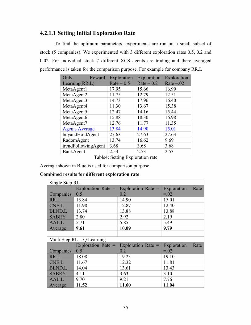


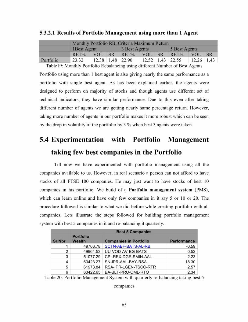


![A Unified Trading Model Based on Robust Optimization for Day … · Robust optimization is suggested in [9] because of the randomness of the wind generation. The above summarized](https://static.documents.pub/doc/80x56/5f375f22261f0b2bb035fcee/a-unified-trading-model-based-on-robust-optimization-for-day-robust-optimization.jpg)


