Automatic Differentiation for Gradient-Based Optimization of Radiatively Heated

Microelectronics Manufacturing Equipment

Christopher D. Moen * and Paul A. Spence t Thermal and Plasma Processes Department

Juan C. Meza 3 and Todd D. Plantenga t Scientific Computing Department

Sandia National Laboratory P.O. Box 969

Livermore, CA 94551-0969

Abstract Automatic differentiation is applied to the op- timal design of microelectronics manufacturing equipment. The performance of nonlinear, least- squares optimization methods is compared between numerical and analytic gradient approaches. The optimization calculations are performed by running large finite-element codes in an object-oriented optimization environment. The Adifor automatic differentiation tool is used to generate analytic derivatives for the finite-element codes. The per- formance results support previous observations that automatic differentiation becomes beneficial as the number of optimization parameters increases. The increase in speed, relative to numerical differences, has a limiting value and results are reported for two different analysis codes.

Introduction There is a great need for equipment and process design optimization in the microelectronics man- ufacturing industry. Manufacturing equipment is becoming more expensive to build and operate as device feature-scales continue to decrease be- low 0.35pm. Sandia has applied computational models and optimization techniques to assist U.S. semiconductor equipment suppliers to develop and improve reactor designs. The equipment of in- terest in this paper is used in thermal processes. Thermal processing plays an important role in manufacturing discrete microelectronic components on silicon wafers. The most important design

*Senior Technical Staff, Member AIAA +Senior Technical Staff $Distinguished Technical Staff

Originally published by American Institute of Aeronautics and Astronautics, 6th AIAAJNASAJISSMO Symposium on Multidisciplinary Analysis and Optimization, September 4-6, 1996, Bellevue, WA.

specification for thermal processing is temperature uniformity. Strict wafer temperature tolerances are crucial to controlling the chemical processes that create material features. Designs optimized for thermal uniformity lead to higher yield and smaller feature scales.

Our automated optimization approach uses the OPT++ object-oriented optimization package’ to generate objective functions and numerical gradients from our finite-element heat transfer code^.^.^ The objective function is formulated using least-squares and is minimized with nonlinear, gradient-based methods. The automated optimization design methods were first demonstrated for rotating-disk reactors4 and later extended to vertical furnaces and rapid thermal processing reactor^.^

Gradients derived from numerical differences (ND) are often inaccurate and become computation- ally expensive when the number of design parame- ters becomes very large, such as calculating optimal heating trajectories.6 Also, the function evaluation is often expensive, requiring on the order of an hour of computer time. Automatic differentiation (AD) is a fast and accurate alternative. Automatic differentiation creates source code for calculating derivatives by applying the derivative chain-rule to an existing code. Gradients from AD are exact so truncation errors in numerical derivatives are eliminated. In particular, we use the Adifor code7 to compute gradient information.

Automatic differentiation is starting to be used to generate sensitivity information for optimization and engineering analysis. Automatic differentiation has been used for sensitivity analysis in simple finite-element structural analysis,s applications to various analysis problem^,^ nonlinear control,1° and creating sparse Jacobian matrices.ll More recently, AD has been applied to a large-scale computational fluid dynamics code12 to generate

sensitivity derivatives for aerodynamic design. We, at Sandia, are applying AD to large-scale radiation heat transfer codes, coupled to object-oriented opti- mization software, to optimize power configurations for thermal processing.

In the following sections, we define a design optimization problem for a vertical batch furnace, present the numerical methods used in the optimiza- tion and analysis codes, and discuss the performance of automatic differentiation in optimization.

Heat Transfer Design Problem The performance of automatic differentiation in design optimization is demonstrated for a vertical, multi-wafer furnace. Vertical furnaces can process up to 200 silicon wafers in a single batch and have been used for thin film deposition, oxidation, and other thermal process steps. Thermal modeling has made particularly important contributions to the design of vertical furnaces.13 The engineering heat transfer models of Houf2 and Badgwell14 were written specifically for the analysis of vertical furnaces. Application of general-purpose, finite- element heat transfer models by Spence15 provided more detailed calculations.

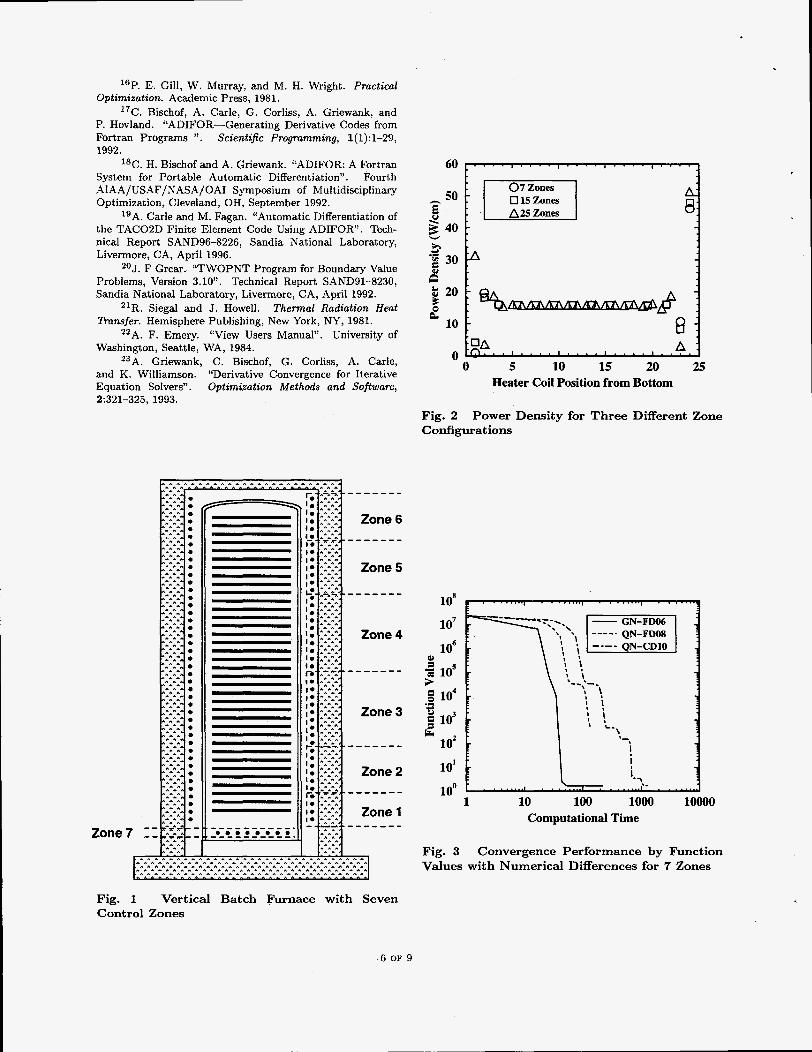
The evolution of vertical furnaces has been driven by the need for process uniformity (i.e., wafer-to-wafer and within-wafer uniformity) and high wafer throughput. A recent variation of the multiwafer reactor design is the small-batch, fast- ramp (SBFR) furnace. The SBFR is designed to heat-up and cool-down quickly, thus reducing cycle time and thermal budget. The SBFR consists of a stack of 50 eight-inch (diameter) silicon wafers enclosed in a vacuum-bearing quartz jar. The stack is radiatively heated by resistive coil heaters contained in an insulated canister. The heating coils can be individually controlled or ganged together in zones to vary the emitted power along the length of the reactor; a seven-zone configuration is shown in Figure 1. There are six control zones (each containing several heating coils) along the length of the furnace and one heater zone in the base. The zones near the ends of the furnace are run hotter than the middle zones to make up for heat loss.

The thermal design optimization problem is: given a discrete number of fixed heating coils, how can the coils be grouped in the fewest number of control zones such that the temperature uniformity about a fixed set-point is maximized. For this paper, we concentrate on finding the optimal power settings and related temperature uniformity for a k e d zone configuration. The objective function, F , is defined by a least-squares fit of the N discrete wafer temperatures, T,,,, to a prescribed profile, Ts,i,

N

F (Pj) = (Tw,z - TS,d2 (1) Z = 1

2 OF

where the p j are the unknown power parameters. The power optimization can be automated while the integer problem of configuring zones is performed in an outer loop.

Numerical Issues The nonlinear, least-squares optimization problem is solved using the quasi-Newton and Gauss-Newton gradient methods16 from the OPT++ library.' The object-oriented software provides optimization classes that are based on the availability of deriva- tives of the objective function. The user only needs to define how the objective function and analytic derivatives (if they exist) are generated. In our case, the information comes from the heat transfer analysis codes. Numerical gradients are generated by OPT++ through multiple evaluations of the objective function.

The derivative-code for generating analytic gradients of the objective function is created from the original finite-element code using the Adifor automatic differentiation a oft ware.^? 1 7 3 The derivative-code returns both the solution variables and their derivatives with respect to the optimiza- tion parameters. The procedure for generating derivative-code with Adifor consists of three steps: code canonicalization, variable nomination, and code generation. In the code canonicalization step, an existing analysis code is rewritten into a standardized format. Adifor produces warnings for non-standard code. In the variable nomination step, Adifor decides which variables are associated with gradient information and generates interaction graphs. In the code generation step, Adifor gen- erates FORTRAN 77 code for generating analytic derivatives.

We generated analytic gradients for two different heat transfer codes applied to vertical furnaces- TWAFER2 and TAC0.3.19 For both codes, we found it quite easy to run the Adifor code by following the steps outlined in the manuaL7 Some work was required in rewriting old "legacy code" to be ANSI-compliant, consisting mostly of data type- casting issues. There were no modifications to the solution procedures.

The TWAFER heat transfer code is an engi- neering code, specific to vertical furnaces. The heat transfer formulation is simplified by using mass lumping and one-dimensional approximations. The nonlinear transport equations are solved using the TWOPNT solver,20 which is a Newton method with a time evolution feature. The TWAFER program has approximately 27000 lines of FORTRAN code and has an image size of 0.9 Mb '. After processing with Adifor for 25 independent variables, the program increases to 39000 lines with an image size of 6.8 Mb.

Compiled on a SGI Power Challenge with -02 flag.

9

DISCLAIMER

This report was prepared as an account of work sponsored by an agency of the United States Government. Neither the United States Government nor any agency thereof, nor any of their employees, makes any warranty, express or implied, or assumes any legal liability or responsibility for the accuracy, completeness, or use- fulness of any information, apparatus, product, or process disclosed, or represents that its usc would not infringe privately owned rights. Reference herein to any spe- cific commercial product, proctss, or service by trade name, trademark, manufac- turer, or otherwise does not necessarily constitute or imply its endorsement, recorn- mendation, or favoring by the United States Government or any agency thereof. The views and opinions of authors exptessed herein do not necessarily state or reflect those of the United States Government or any agency thereof.

DISCLAIMER

Portions of this document may be illegible electronic image products. Images are produced from the best available original document.

Detailed finite-element simulations are per- formed with the TACO heat transfer code. Radiant exchange between enclosure surfaces is based on the net radiation method.21 View factors for the enclosure radiation exchange are computed using VIEWC.22 The finite-element thermal simulations of the SBFR use 1500 nodes and three enclosures with a total of 500 surfaces. The surfaces are treated as diffuse gray and the semi-transparency of the quartz window is approximated using enclosure averaging. The nonlinear transport equations are solved iteratively using time marching with a skyline-LDU decomposition. The TACO program has approximately 12800 lines of FORTRAN code and an image size of 9.3 Mb. After processing with Adifor for 25 independent variables, the program increases to 20000 lines with an image size of 210 Mb.

Examde Problems The performance of analytic gradients versus numer- ical gradients is explored using both the TWAFER code and the TACO code. The goal is to study the behavior of the methods as the number of parameters grows. In all cases, the objective is to optimize the heater zone powers in order to bring the wafer temperatures as close to 1300 K as possible.

The power optimization problems are solved with either the quasi-Newton method (QN) or the Gauss-Newton (GN) method, both with trust region search algorithms. Different numerical difference accuracies are used to characterize the performance of numerical gradients. Forward differences were tested with a function accuracy of (FD06) and lo-* (FD08). Central differences were tested with a function accuracy of (CD10). The function accuracy determines the step size for numerical differences.

(CD06) and

TWAFER: Power Optimization

There are many different parameter combina- tions considered in the study of the TWAFER code. There are three different heater zone configurations: 7 zones, 15 zones, and 25 zones. There is always one bottom heater and the rest are equally-sized side heaters. In addition, both the QN and GN algorithms were tested with the full suite of function accuracies. Convergence plots for the 7- zone problem are included to demonstrate typical behavior. Results for the 15 and %-zone problems are tabulated since they exhibit behavior similar t o the 7-zone problem.

The initial guess at the powers is 4.8 kW, distributed evenly between the side heaters. The bottom heater power is the same power as a side heater. The optimization terminates when the norm of the gradient of the objective function goes below

or when the change in the value of the objective function becomes less than

The resulting power distribution is characterized by a large central flat zone with temperature variations at the ends. The optimal power densities are shown in Figure 2. The root-mean-square temperature variation across the stack for 7 power zones is is less than 0.1 K and the maximum temperature differs only by 1 K from the target temperature. The uniformity is even better for the 25-zone configuration because it can adapt to the heat losses at the ends of the furnace.

TWAFER Numerical Gradient Performance

Of the two optimization methods, Gauss- Newton converges much faster than quasi-Newton with little sensitivity to errors in the gradient. A plot of the function value with respect to computational time is shown in Figure 3 for numerical gradients. The use of central differences with the GN method has no benefit and results in convergence times twice as long as forward differences. The QN method with numerical gradients is very sensitive to the accuracy of the gradients. The use of forward differences results in premature termination of the optimization when the trust region becomes too small to advance the solution. Central differences with a function accuracy of are required in order to generate gradients accurate enough for QN to work.

The optimization problem is ill-conditioned. Large variations in power near the ends of the furnace result in only small changes in temperature. The condition number of the approximate Hessian used for the Gauss-Newton method is on the order of lo9. The quasi-Newton method has a difficult time converging for ill-conditioned problems and is very sensitive to truncation errors in the numerical differences. With- numerical differences, QN only achieves a condition number of lo6 before failing because of the trust region size. With analytic .gradients, the QN method converges and the condition number does reach lo9.

The lz-norm of the gradient is an indication of how close the solution is to optimal and a plot of the gradient norms is shown in Figure 4. The oscillation in the gradient norm for the QN method corresponds to the stair-stepping in the function value. The QN method is taking several steps in directions very close to one another. A sudden drop in function value corresponds to a large change in search direction. The gradient builds up in size before each direction change, indicating that the solution might be better advanced by just taking the steepest decent.

TWAFER: Analytic Gradient Performance

Adifor is applied to TWAFER to generate a code called AD-TWAFER that returns both the function value and the gradient. The convergence rate of the GN and QN methods with analytic gradients is compared to the fastest numerical

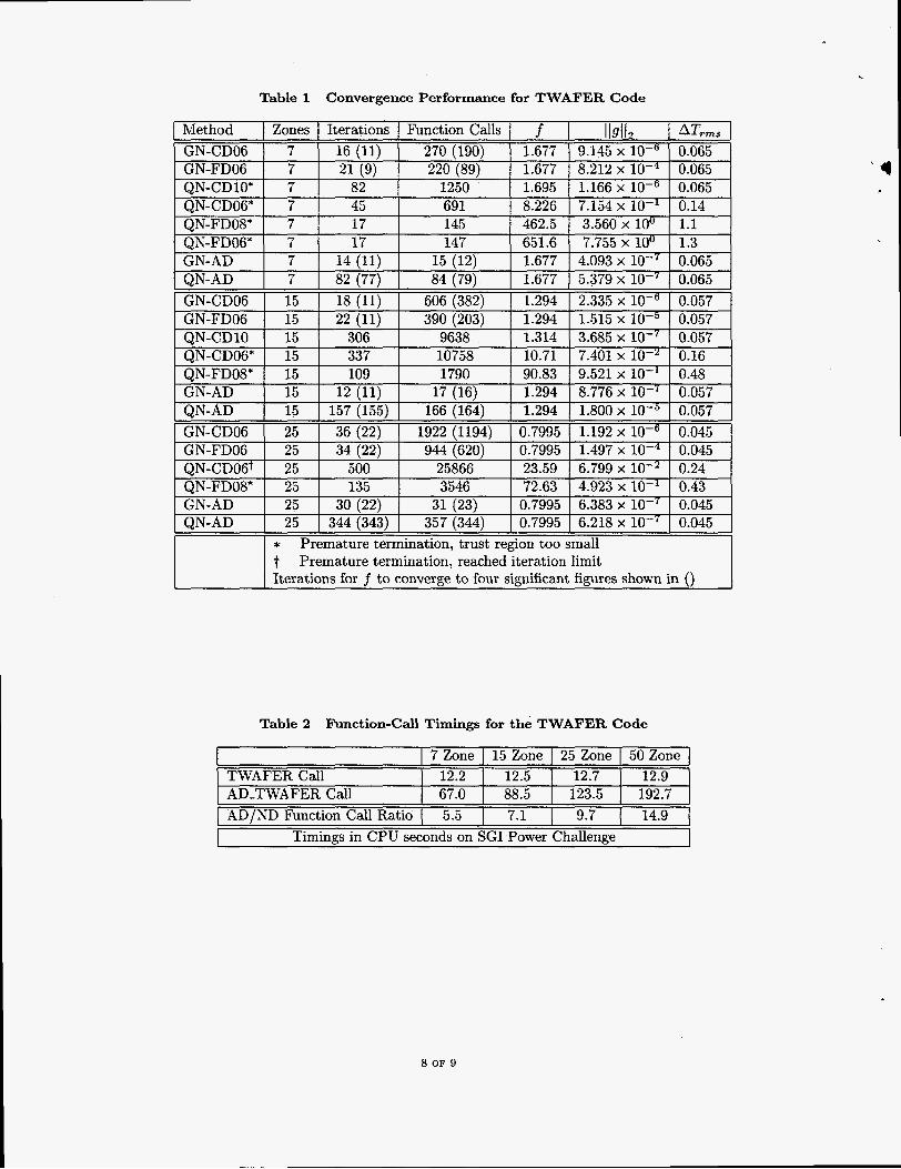
gradient method (GN with forward differences) in Figure 5. The GN method with analytic derivatives is faster than numerical gradients by a factor of 1.6 for seven parameters. The QN method continues to be slow, but the method does converge since the gradients are exact. The convergence of the ln-norm of the gradient is shown in Figure 6. A tabulation of convergence information for all three zone configurations is included in Table 1.

TWAFER. AD Scaling

The performance of AD, relative to ND with the Gauss-Newton method, improves as the number of optimization parameters increases. The compu- tational work required to form gradients with AD becomes less, relative to ND, and the supporting TWAFER function-call timings are given in Table 2. The first row of the table lists the average CPU time required to complete one function evaluation with TWAFER. The second row of the table lists the average CPU time required to calculate the function value and analytic gradient with AD-TWAFER.

Whereas the TWAFER code runs the same no matter how many power zones are used, the work required by AD-TWAFER appears to scale linearly with the number of independent parameters, shown in the third row of Table 2. The slope of the growth rate of AD (normalized by an ND call) with respect to the slumber of parameters is 0.2, shown in Figure 7. The performance of AD over ND improves with the number of parameters, but at a diminishing rate. The performance ratio compares the work required to take one Newton step. The AD/ND performance ratio asymptotes to 0.2. For the TWAFER code using GN, the largest improvement in convergence we expect to see is a factor of five.

TACO: AD Scaling

It is difficult t o assess the performance of analytic derivatives in the TACO code because the computational work required for each function evaluation is extremely dependent on the starting temperature guess. Each function evaluation consists of time-marching the governing equations to steady-state, and requires anywhere from 500 to 3500 seconds of CPU time. The solution of the enclosure radiation problem by Gauss-Seidel iteration also complicates the overall evaluation.

The largest change in temperature from the actual solution to the transport equations occurs after each Newton step when the powers are up- dated. It is computationally expensive to generate gradients during the time iteration to steady state. This fact was noted pre~iously'~ and efficiency can be improved by using simplified recurrence differentiati0n.2~ As an alternative, we found it useful to first update the solution with the standard

TACO code after each optimization step, before time marching with the analytic gradient code.

The AD parameter scaling is estimated based on the work involved in taking a single time step in the TACO code. A time step involves loading a coefficient matrix, loading a forcing function, and inverting the linear system. The matrix and forcing function may be reformed many times during a sub-iteration process to advance one time step. In addition, each time the forcing function is formed, the enclosure radiation problem must be solved. The matrix and forcing function calculations require the bulk of the CPU time with very little time required for the matrix inversion.

The CPU times required for the different calculations required in a time step are listed in Table 3. The CPU time required for a time step in the standard version of TACO is the same, regardless of the number of parameters. The timings have been broken out into the CPU time to load the matrix, the CPU time to evaluate the forcing function, and the overall CPU time to take the time step. It turns out that the analytic derivatives are more expensive than forward differences until there are at least 16 optimization parameters. Even then, the limiting speed-up appears to be only two times faster than numerical derivatives.

As the number of independent variables shrinks towards zero, the Adifor-generated code does not run as fast as the original code. The automatic differentiation adds overhead to the analysis codes, mainly through external loops over the independent variables. As a result, there is a threshold number of variables for which automatic differentiation be- comes more expensive than numerical differencing. The threshold points for both TACO and TWAFER are illustrated in Figure 7, a plot of how the computational work scales with the number of parameters.

Concluding Remarks Gradient-based optimization methods were applied to the design of power configurations in a vertical furnace. The performance using analytic gradients was compared to numerical gradients for two different optimization algorithms.

0 For nonlinear, least-squares optimization prob- lems with numerical gradients, the Gauss- Newton method is much more robust than the quasi-Newton, even though Gauss-Newton is more expensive per nonlinear step.

0 The Gauss-Newton gradient method is not very sensitive to numerical difference truncation errors.

0 The analytic gradients are much more accurate than numerical gradients. The performance of the quasi-Newton method is the best indicator

4 OF 9

of the difference between the two approaches for generating gradients. The quasi-Newton method rarely convergences when numerical dif- ferences are used, even central differences. The method will converge when analytic gradients are used.

0 For the TWAFER code with the Gauss-Newton optimization method, the AD gradients lead to faster convergence than numerical gradients, but the rate ratio asymptotes to a factor of five.

0 For the TACO code, the AD gradients are slower than forward differences until a break- even point of 16 parameters. For a large number of parameters, the AD gradients are faster, but the acceleration factor asymptotes to a factor of two.

0 Given the computer memory resources, it is always favorable to use AD gradients for optimization with the TWAFER code. The TACO code has too large a benefit threshold to warrant using analytic gradients for most of the problems we are interested in. The acceleration factor and threshold for the TACO code can probably be improved by changing the solution strategy for the transport equations and enclosure radiation problem.

To date, we have only considered parameter optimization based on thermal issues. Future work looks towards shape optimization based on material deposition criteria. The material deposition rate and uniformity are computed using reacting Aow models with conjugate heat transfer. The shape optimization is expected to be very expensive because of the radiation transport processes. Each shape variation results in recalculating radiation view factors. Using numerical gradients increases the number of view factor calculations that must be performed.

Acknowledgements We would like to thank Alan Carle and Mike Fagan of Rice University for their assistance in applying Adifor to our heat transfer codes. This work was funded by the Department of Energy under a Laboratory-Directed Research and Development program.

References

References ‘J. C. Meza. “OPT++: An Object-Oriented Class

Library for Nonlinear Optimization”. Technical Report SAND94-8225, Sandia National Laboratory, Livermore, CA, March 1994.

2W. G. Houf, J . F. Grcar, and W. G. Breiland. “A Model for Low Pressure Chemical Vapor Deposition in a Hot- Wall Tubular Reactor”. Materials Science Engineering, B, Solid State Materials for Advanced Technology, 17(1/3):163- 171, February 1993.

“TAC03D - A Three-Dimensional Finite Element Heat Transfer Code”. Technical Report SAND83-8212, Sandia National Laboratory, Livermore, CA, April 1983.

4C. D. Moen, P. A. Spence, and J. C. Meza. “Optimal Heat Transfer Design of Chemical Vapor Deposition Reactors”. Technical Report SAND95-8223, Sandia National Laboratory, Livermore, CA, April 1995.

5P. A. Spence, W. S. Winters, R. J. Kee, and A. Kermani. “The Application of Computational Simulation to Design Optimization of an Axisymmetric Rapid Thermal Processing System”. In 2nd International Rapid Thermal Processing Conference, Monterey, CA, pages 139-145, Au- gust 1994.

6J. C. Meza and T. D. Plantenga. “Optimal Control of a CVD Reactor for Prescribed Temperature Behavior”. Technical Report SAND95-8224, Sandia National Laboratory, Livermore, CA, April 1995.

‘C. Bischof, A. Carle, P. Hovland, P. Khademi, and A. Mauer. “ADIFOR 2.0 User’s Guide”. Technical Report CRPC-TR95516-S, Rice University, Houston, TX, March 1995. Revised: May 1995. Also available as ANL/MCS-TM- 192, Argonne National Laboratory.

“Higher-Order Sensitivity Analysis of Finite Element Method by Automatic Differentiation”. Computational Mechanics, 16(4):223-234, July 1995.

9S. Chinchalkar. “The Application of Automatic Differentiation to Problems in Engineering Analysis”. Com- puter Methods in Applied Mechanics and Engineering, 118(1/2):197-207, September 1994.

loS. L. Campbell, E. Moore, and Y. Zhong. “Utilization of Automatic Differentiation in Control Algorithms”. ZEEE lhnsactions on Automatic Control, 39(5):1047-1052, May 1994.

”B. M. Averick, J. J. More, C. H. Bischof, A. Carle, and A. Griewank. “Computing Large Sparse Jacobian Matrices Using Automatic Differentiation”. SIAM Journal of Scientific Computing, 15(2):285-294, 1994.

12L. L. Green, P. A. Newman, and K. J. Haigler. “Sensitivity Derivatives for Advanced CFD Algorithm and Viscous Modeling Parameters via Automatic Differentiation”. Journal of Computational Physics, 125:313-324, 1996.

I3T. A. Badgwell, T. Breedijk, S. G . Bushman, S. W. Butler, S. Chatterjee, T. F. Edgar, A. J. Toprac, and I. Trachtenberg. “Modeling and Control of Microelectronics Material Processing”. Computers in Chemical Engineering, 19(1):1-41, January 1995.

‘*T. A. Badgwell, I. Trachtenberg, and T. F. Edgar. “Modeling the Wafer Temperature Profile in a Multiwafer LPCVD Furnace”. Journal of the Electrochemical Society, 141 ( 1 ) : 161-1 72, January 1994.

15P. A. Spence, W. G. Houf, J . F. Grcar, R. J. Kee, R. S. Larson, W. G. Breiland, H. K. Moffat, and M. E. Coltrin. “The Development and Application of Computational Simulation to Hot-Wall Multiple-Wafer Low- Pressure Chemical Vapor Deposition Diffusion Furnaces”. Technical Report SETEC93-037, Sandia National Laboratory, Livermore, CA, January 1993. Prepared for Sematech, Austin, TX. Limited Distribution.

3W. E. Mason.

Osaki, F. Kimura, and M. Berz.

16P. E. Gill, W. Murray, and M. H. Wright. Practical Optimization. Academic Press, 1981.

“C. Bischof, A. Carle, G. Corliss, A. Griewank, and P. Hovland. “ADIFOR-Generating Derivative Codes from Fortran Programs ”. Scientific Progmmming, 1( 1):1-29, 1992.

I8C. H. Bischof and A. Griewank. “ADIFOR: A Fortran System for Portable Automatic Differentiation”. Fourth AIAA/USAF/NASA/OAI Symposium of Multidisciplinary Optimization, Cleveland, OH, September 1992.

19A. Carle and M. Fagan. “Automatic Differentiation of the TACO2D Finite Element Code Using ADIFOR”. Tech- nical Report SAND96-8226, Sandia National Laboratory, Livermore, CA, April 1996.

2oJ. F Grcar. “TWOPNT Program for Boundary Value Problems, Version 3.10”. Technical Report SAND91-8230, Sandia National Laboratory, Livermore, CA, April 1992.

21R. Siegal and J. Howell. Thermal Radiation Heat Tmnsfer. Hemisphere Publishing, New York, NY, 1981.

22A. F. Emery. “View Users Manual”. University of Washington, Seattle, WA, 1984.

23A. Griewank, C. Bischof, G. Corliss, A. Carle, and K. Williamson. “Derivative Convergence for Iterative Equation Solvers”. Optimization Methods and Software, 2:321-325, 1993.

Zone

50

40

h

E

s 2 30 .C

a” 5 20 B

10 rE

Fig. 2 Configurations

Power Density for Three Different Zone

10’

lo6 3 io5 g io4 5 io3

lo2

10’

loo

8

* .I c)

k

1 10 100 1000 10000 Computational Time

Fig. 3 Values with Numerical Differences for 7 Zones

Convergence Performance by Function

Fig. 1 Vertical Batch Furnace with Seven Control Zones

6 OF 9

10’ lo4 lo3

E 10’ 2 10’ i$ loo 3 10-1

6 lo-’ i o 3 lo4 lo-’

Fig. 4

10 100 1000 10000 Computational Work

Convergence Performance by Gradient Norms with Numerical Differences for 7 Zones

g io4 2 io3

lo’

.I U

Lu

10’

loo 1 10 100 1000

Computational Time

los 104 103

E 10’ 10’

3 loo 3 1 0 - I

h

a lo-’ 105 104 10”

Fig. 6 Norm

1 10 100 1000 Computational Work

Convergence Performance by Gradient with Automatic Differentiation for 7 Zones

Fig. 5 Convergence Performance by Function Value with Automatic Differentiation for 7 Zones

Method GN-CDO6 GN-FDO6

* t Iterations for f to converge to four significant figures shown in ()

Premature termination, trust region too small Premature termination, reached iteration limit

Zones Iterations Function Calls f 1191 12 AT,,, 7 16 (11) 270 (190) 1.677 9.145 x 0.065 7 21 f9) 220 (89) 1.677 8.212 x 0.065

TWAFER Call AD-TWAFER Call AD/ND Function Call Ratio

I I I I I

Timings in CPU seconds on SGI Power Challenge

7 Zone 15 Zone 25 Zone 50 Zone 12.2 12.5 12.7 12.9 67.0 88.5 123.5 192.7 5.5 7.1 9.7 14.9

8 OF 9

25

TACO/Matrix

TACO/Time Step TACO/Force Vector

AD-TACO/Matrix AD-TACO/Force Vector AD-TACO/Time Step

I ' * " I " " I ' " '

AD-TWAFER

5 Zone 9 Zone 15 Zone 25 Zone 0.1 0.1 0.1 0.1 0.17 0.17 0.17 0.17 5.8 5.8 5.8 5.8 0.96 1.08 1.36 1.89 1.35 1.75 2.34 3.12 62.1 79.4 96.3 130.3

0 5 10 15 20 Number of Parameters

Fig. 7 Analytic Gradients Accelerate Convergence of Optimization Algorithms

Table 3 Function-Call Timings for the TACO Code