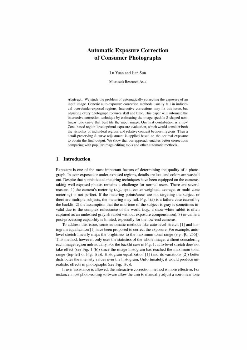
Automatic Exposure Correction of Consumer Photographs Lu Yuan and Jian Sun Microsoft Research Asia Abstract. We study the problem of automatically correcting the exposure of an input image. Generic auto-exposure correction methods usually fail in individ- ual over-/under-exposed regions. Interactive corrections may fix this issue, but adjusting every photograph requires skill and time. This paper will automate the interactive correction technique by estimating the image specific S-shaped non- linear tone curve that best fits the input image. Our first contribution is a new Zone-based region-level optimal exposure evaluation, which would consider both the visibility of individual regions and relative contrast between regions. Then a detail-preserving S-curve adjustment is applied based on the optimal exposure to obtain the final output. We show that our approach enables better corrections comparing with popular image editing tools and other automatic methods. 1 Introduction Exposure is one of the most important factors of determining the quality of a photo- graph. In over-exposed or under-exposed regions, details are lost, and colors are washed out. Despite that sophisticated metering techniques have been equipped on the cameras, taking well-exposed photos remains a challenge for normal users. There are several reasons: 1) the camera’s metering (e.g., spot, center-weighted, average, or multi-zone metering) is not perfect. If the metering points/areas are not targeting the subject or there are multiple subjects, the metering may fail. Fig. 1(a) is a failure case caused by the backlit; 2) the assumption that the mid-tone of the subject is gray is sometimes in- valid due to the complex reflectance of the world (e.g., a snow-white rabbit is often captured as an undesired grayish rabbit without exposure compensation); 3) in-camera post-processing capability is limited, especially for the low-end cameras. To address this issue, some automatic methods like auto-level stretch [1] and his- togram equalization [1] have been proposed to correct the exposure. For example, auto- level stretch linearly maps the brightness to the maximum tonal range (e.g., [0, 255]). This method, however, only uses the statistics of the whole image, without considering each image region individually. For the backlit case in Fig. 1, auto-level stretch does not take effect (see Fig. 1 (b)) since the image histogram has reached the maximum tonal range (top-left of Fig. 1(a)). Histogram equalization [1] (and its variations [2]) better distributes the intensity values over the histogram. Unfortunately, it would produce un- realistic effects in photographs (see Fig. 1(c)). If user assistance is allowed, the interactive correction method is more effective. For instance, most photo editing software allow the user to manually adjust a non-linear tone
Abstract. We study the problem of automatically correcting the exposure of aninput image. Generic auto-exposure correction methods usually fail in individ-ual over-/under-exposed regions. Interactive corrections may fix this issue, butadjusting every photograph requires skill and time. This paper will automate theinteractive correction technique by estimating the image specific S-shaped non-linear tone curve that best fits the input image. Our first contribution is a newZone-based region-level optimal exposure evaluation, which would consider boththe visibility of individual regions and relative contrast between regions. Then adetail-preserving S-curve adjustment is applied based on the optimal exposureto obtain the final output. We show that our approach enables better correctionscomparing with popular image editing tools and other automatic methods.
1 Introduction
Exposure is one of the most important factors of determining the quality of a photo-graph. In over-exposed or under-exposed regions, details are lost, and colors are washedout. Despite that sophisticated metering techniques have been equipped on the cameras,taking well-exposed photos remains a challenge for normal users. There are severalreasons: 1) the camera’s metering (e.g., spot, center-weighted, average, or multi-zonemetering) is not perfect. If the metering points/areas are not targeting the subject orthere are multiple subjects, the metering may fail. Fig. 1(a) is a failure case caused bythe backlit; 2) the assumption that the mid-tone of the subject is gray is sometimes in-valid due to the complex reflectance of the world (e.g., a snow-white rabbit is oftencaptured as an undesired grayish rabbit without exposure compensation); 3) in-camerapost-processing capability is limited, especially for the low-end cameras.
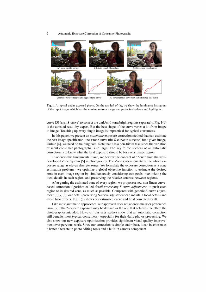
To address this issue, some automatic methods like auto-level stretch [1] and his-togram equalization [1] have been proposed to correct the exposure. For example, auto-level stretch linearly maps the brightness to the maximum tonal range (e.g., [0, 255]).This method, however, only uses the statistics of the whole image, without consideringeach image region individually. For the backlit case in Fig. 1, auto-level stretch does nottake effect (see Fig. 1 (b)) since the image histogram has reached the maximum tonalrange (top-left of Fig. 1(a)). Histogram equalization [1] (and its variations [2]) betterdistributes the intensity values over the histogram. Unfortunately, it would produce un-realistic effects in photographs (see Fig. 1(c)).
If user assistance is allowed, the interactive correction method is more effective. Forinstance, most photo editing software allow the user to manually adjust a non-linear tone
2 Automatic Exposure Correction of Consumer Photographs
(d) interactive correction and applied tone curve (e) our automatic correction and estimated tone curve
Fig. 1. A typical under-exposed photo. On the top-left of (a), we show the luminance histogramof the input image which has the maximum tonal range and peaks in shadows and highlights.
curve [3] (e.g., S-curve) to correct the dark/mid-tone/bright regions separately. Fig. 1(d)is the assisted result by expert. But the best shape of the curve varies a lot from imageto image. Touching up every single image is impractical for typical consumers.
In this paper, we present an automatic exposure correction method that can estimatethe best image specific non-linear tone curve (the S-curve in our case) for a given image.Unlike [4], we need no training data. Note that it is a non-trivial task since the variationof input consumer photographs is so large. The key to the success of an automaticcorrection is to know what the best exposure should be for every image region.
To address this fundamental issue, we borrow the concept of “Zone” from the well-developed Zone System [5] in photography. The Zone system quantizes the whole ex-posure range as eleven discrete zones. We formulate the exposure correction as a zoneestimation problem - we optimize a global objective function to estimate the desiredzone in each image region by simultaneously considering two goals: maximizing thelocal details in each region, and preserving the relative contrast between regions.
After getting the estimated zone of every region, we propose a new non-linear curve-based correction algorithm called detail-preserving S-curve adjustment, to push eachregion to its desired zone, as much as possible. Compared with generic S-curve adjust-ment [6][7][8], our detail-preserving S-curve adjustment can maintain local details andavoid halo effects. Fig. 1(e) shows our estimated curve and final corrected result.
Like most automatic approaches, our approach does not address the user preferenceissue [9]. The “correct” exposure may be defined as the one that achieves the effect thephotographer intended. However, our user studies show that an automatic correctionstill benefits most typical consumers - especially for their daily photos processing. Wealso show our new exposure optimization provides significant visual quality improve-ment over pervious work. Since our correction is simple and robust, it can be chosen asa better alternate in photo editing tools and a built-in camera component.
Automatic Exposure Correction of Consumer Photographs 3
2 Related Work
Automatic exposure control is one of the most essential research issues for cameramanufacturers. The majority of developed techniques are hardware-based. Representa-tive work include HP “Adaptive Lighting” technology [10] , Nikon “D-Lighting” tech-nology [11]. These methods compress the luminance range of images by a known tonemapping curve (e.g., Log curve) and further avoid local contrast distortion by “Retinex”processing [12]. Specific hardware has been designed to perform per-pixel exposurecontrol [13] or scene-based (e.g., backlit, frontlit [14] or face [15]) exposure control.Some automatic techniques (e.g. [16]) are proposed to estimate the optimal exposureparameters (shutter speed and aperture) during taking photos.
There are numerous techniques about software-based exposure adjustment, includ-ing most popular global correction (e.g., auto-level stretch, histogram equalization [1])and local exposure correction [17][18]. However, these methods only use some heuris-tic histogram analysis to map per-pixel exposure to the desired one, without consideringthe spatial information of pixels (or regions). An interesting work [19] tries to enhance-ment image via frequency domain (i.e., block DCT). But some fixed tone curves areused for each image and blocking artifacts occasionally occur in their results.
Some algorithms [8][20] only consider the exposure of the regions of interest (ROI)and assume it is most important to the whole image correction. Different from ours,they use a known and predefined tone curve but we will estimate the specific curve forevery image. Some tone mapping algorithms [21] can also be used to estimate the key ofscene and infer a tone curve to map its original exposure to the desired key. However, thekey estimation is based on the global histogram analysis and is sometimes inaccurate.Exposure fusion [22] combines well-exposed regions together from an image sequencewith bracketed exposures. In contrast, we only use a single image as the input.
Since the exposure correction is kind of subjective, recent methods [23][4][9] en-hance the input image using training samples from internet or personalized photos.However, our exposure correction is not relied on the selection of training images andonly focuses on the input image itself. Another issue worth mentioning is that our ap-proach does not aim to restore completely saturated pixels like [24].
3 Automatic Exposure Correction Pipeline
Our exposure correction pipeline is depicted in Fig. 2 and divided to two main steps:exposure evaluation and S-curve adjustment. Both components are performed in theluminance channel. To avoid bias due to different camera metering systems, or user’smanual settings, we would linearly normalize the input tonal range to [0, 1] at first.
The heart of our system is an optimization-based, region-level exposure evaluation(see Section 4). In the exposure evaluation, we apply a Zone-based exposure analysisto estimate the desired zone (i.e., exposure) for each image region. We first segment theinput image into individual regions (i.e., super-pixels). In each region, we measure vis-ible details, region size, and relative contrast between regions. Then we formulate theoptimal zone estimation as a global optimization which takes into account all these fac-tors. We also use the high level information (e.g., face) to set the priority of the regions.
4 Automatic Exposure Correction of Consumer Photographs
After the exposure evaluation, we estimate a best non-linear curve (S-curve) mappingfor the entire image to push each region to its optimal zone. We further introduce adetail-preserving S-curve adjustment (see Section 5) instead of naıve S-curve mappingto preserve local details and suppress halo effects in the final result.
4 Region-level Exposure Evaluation
The aim of our exposure evaluation is to infer the image specific tone curve for theconsequent detail-preserving S-curve adjustment. To achieve this goal, we first need toknow what is the “best” exposure of each region and how to estimate them all together.
4.1 Zone region
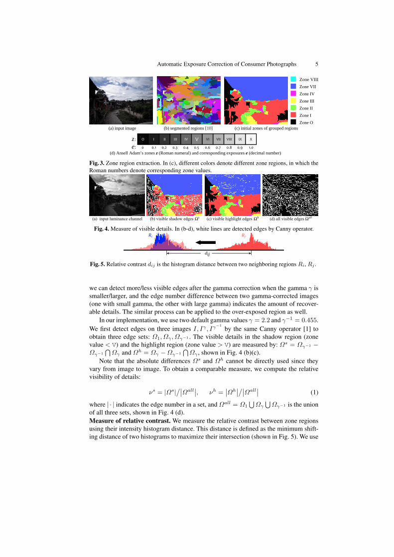
To measure the exposure, we borrow the concept of “Zone” from Ansel Adams’ ZoneSystem [5], which is shown in Fig. 3(d). In Zone System, the entire luminance range [0,1] is equally divided into 11 zones, ranging from O to X denoted by Roman numbers,with O representing black, V middle gray, and X pure white; these values are known aszones. In each zone, the mean intensity value is referred as its corresponding exposure.This concept was also used in recent HDR tone mapping applications [21][25] andrealistic image composition [26].
We represent the image by a number of zone regions. We first decompose the imageinto a set of regions by graph-based segmentation [27]. Each region falls into one of thezones. Then, we merge the neighboring regions with the same zone value. To extracthigh-level information (e.g., face/sky) for high priority of adjustment, we need to detectfacial regions [28] and sky regions [29]. All connected regions belonging to face/skyregions are also merged. We call the final merged region as “zone region”. Fig. 3(a-c)shows the procedure of the zone region extraction.
4.2 Optimal zones estimation
The optimal zone estimation can be formulated as a global optimization problem byconsidering two aspects: maximizing the visual details and preserving the original rel-ative contrast between neighboring zone regions.Measure of visible details. The amount of visible details in under-/over-exposed re-gions can be measured by the difference of the detected edges in these images whichare generated by applying different gamma-curves on the input image I (the process isdenoted as Igamma = Iγ). It is based on an observation: in an under-exposed region,
Automatic Exposure Correction of Consumer Photographs 5
(a) input image (b) segmented regions [10] (c) initial zones of grouped regions
Zone VII
Zone O
Zone VIII
Zone IIZone IIIZone IV
Zone I
O I II III IV V VI VII VIII IX X
0 0.1 0.2 0.3 0.4 0.5 0.6 0.7 0.8 0.9 1.0
::
ze
(d) Ansell Adam’s zones z (Roman numeral) and corresponding exposures e (decimal number)
Fig. 3. Zone region extraction. In (c), different colors denote different zone regions, in which theRoman numbers denote corresponding zone values.
Fig. 4. Measure of visible details. In (b-d), white lines are detected edges by Canny operator.Ri Rj
ijd
Fig. 5. Relative contrast dij is the histogram distance between two neighboring regions Ri, Rj .
we can detect more/less visible edges after the gamma correction when the gamma γ issmaller/larger, and the edge number difference between two gamma-corrected images(one with small gamma, the other with large gamma) indicates the amount of recover-able details. The similar process can be applied to the over-exposed region as well.
In our implementation, we use two default gamma values γ = 2.2 and γ−1 = 0.455.We first detect edges on three images I, Iγ , Iγ
−1
by the same Canny operator [1] toobtain three edge sets: Ω1, Ωγ , Ωγ−1 . The visible details in the shadow region (zonevalue < V) and the highlight region (zone value > V) are measured by: Ωs = Ωγ−1 −Ωγ−1
⋂Ωγ and Ωh = Ωγ −Ωγ−1
⋂Ωγ , shown in Fig. 4 (b)(c).
Note that the absolute differences Ωs and Ωh cannot be directly used since theyvary from image to image. To obtain a comparable measure, we compute the relativevisibility of details:
νs = |Ωs|/∣∣Ωall∣∣, νh =
∣∣Ωh∣∣/∣∣Ωall∣∣ (1)
where | · | indicates the edge number in a set, and Ωall = Ω1
⋃Ωγ⋃Ωγ−1 is the union
of all three sets, shown in Fig. 4 (d).Measure of relative contrast. We measure the relative contrast between zone regionsusing their intensity histogram distance. This distance is defined as the minimum shift-ing distance of two histograms to maximize their intersection (shown in Fig. 5). We use
6 Automatic Exposure Correction of Consumer Photographs
the term “relative contrast” for this distance. For example, when their histograms aretoo close, we say their relative contrast is small.Zones estimation as an optimization. With the two measures defined, we formulatethe best zone estimation as a graph-based labeling problem. Each zone region is regard-ed as a node and any two neighboring zone regions are connected by a link. The optimallabels Z = z∗i of nodes are the final desired zones. We define the Markov RandomField (MRF) energy function E(Z) of the graph as:
Z∗ = argminZE(Z) = argmin
Z(∑
iEi + λ
∑i,jEij),
where Ei is the data term of an individual region i, and Eij is the pairwise term be-tween two adjacent regions i and j. In our work, the data term and pairwise term arerespectively specified by the form: Ei = −log(P (i)) and Eij = −log(P (i, j)).
The likelihood P (i) of a region i is measured by its visibility of details νi, theregion size Ci (normalized by the whole image size), and the important region size θi(normalized by the whole image size). The important region is directly computed fromthe probability map of facial/sky detector. We take into account all the three factors:
where zi is the original zone, zi is the new zone and ρ(t) = 1/ (1 + exp(−t)) is asigmoid function. The likelihood would encourage shadow/highlight regions to moveto higher/lower zones. For mid-zones (zone V), it takes no effect.
The coherence P (i, j) is defined by the change of relative contrast between twoneighboring regions, from the original relative contrast dij (before the optimization) tothe new relative contrast dij (after the optimization), which is denoted by
P (i, j) = Cj × G(dij − dij), (3)
where G(·) is a zero-mean gaussian function with variance 0.15 and the weight Cj isused so that relatively smaller regions contribute less. The coherence would penalizethe dramatic change of relative contrast.
To obtain the global optimum, we use a brute-force searching method to travel allcombinations of zone candidates for all regions because the total number of zone re-gions is not very high after region merging. To automatically estimate the weight λ, wefirst calculate the sum of data terms and the sum of pairwise terms across all combi-nations of zone candidates. Then we set λ to the ratio of two summations. We found itworks very well in our experiments and does not require any tuning.
5 Detail-preserving S-curve Adjustment
After getting the optimal zone for every region, we might have mapped the zone val-ue (i.e., exposure) of each region to its desired zone individually. However, this localmapping has the risk to produce exposure distortion in relatively small regions becausethese regions often contain insufficient information to estimate their optimal zones. To
Automatic Exposure Correction of Consumer Photographs 7
0 0.1 0.2 0.3 0.4 0.5 0.6 0.7 0.8 0.9 10
0.1
0.2
0.3
0.4
0.5
0.6
0.7
0.8
0.9
1
0 0.1 0.2 0.3 0.4 0.5 0.6 0.7 0.8 0.9 10
0.1
0.2
0.3
0.4
0.5
amount : 100%
amount : 60%
amount : 30%
s
h
(a) (b)
input intensity
outp
ut in
tens
ity
input intensity
outp
ut in
tens
ity
Fig. 6. (a) S-curve, φs, φh control the magnitude of S-curve adjustment in the shadow range andthe highlight range respectively. (b) the curves of f∆(x) weighted by different amount φ.
address this issue, we use a non-linear tone curve to globally map the brightness of ev-ery pixel to its desired exposure. We further preserve local contrast by fusion betweenthe global curve mapping and an adaptive local detail enhancement.S-curve adjustment. Most photographers often use an S-shaped non-linear curve (S-curve) to manually adjust the exposure in shadow/mid-tone/highlight areas. Fig. 6 (a)shows a typical (inverse) S-curve. This kind of S-curve can be simply parameterized bytwo parameters: shadow amount φs and highlight amount φh, which is denoted by:
f(x) = x+ φs × f∆(x)− φh × f∆(1− x), (4)
where x and f(x) are the input and output pixel intensities. f∆(x) is the incrementalfunction and empirically defined as: f∆(x) = κ1x exp (−κ2xκ3), where κ2 and κ3control the modified tone range of the shadows or highlights. We use the default param-eters (κ1 = 5, κ2 = 14, κ3 = 1.6) of f∆(x) to make the modified tonal range fall in[0, 0.5]. The effect of shadow/highlight amounts (φs, φh) is shown in Fig. 6 (b).Inference of correction amounts. We infer the amounts (φs, φh) from the estimatedoptimal zone in every region. For the shadow regions, we want to set the amount φs sothat the original zone value of each shadow region can be moved to its optimal zonevalue, as much as possible. The amount φh can be estimated in a similar way.
Suppose the original exposure and new exposure of a shadow region i are respec-tively ei and ei. (The relationship between the exposure and its corresponding zonevalue is shown on Fig. 3(d)). The original exposure is calculated by the intensity mean:ei =
∑I/ci, where I is original intensity and ci is the region size. After the S-curve
adjustment (by Eqn. 4), the new exposure ei =∑f(I)/ci =
∑(I + φs × f∆(I))/ci.
Thus, the shadow amount φs of this region should be: φs = (ei − ei)× ci ×∑f∆(I).
To consider all regions, we take the weighted average of the estimated shadow amountsof all regions. We use the percentage of region size as the weight.Detail-preserving S-curve adjustment. If we directly apply the S-curve mapping (inEqn. 4) to the input image, we may lose local details. Fig. 7(b) shows such a case,where the result looks too flat although dark areas are lightened. This undesired effectis due to: moving the intensities from shadows and highlights to the middle will com-press the mid-tones. Since the S-curve is usually monotonic, the contrast between twoneighboring pixels in the mid-tones could be reduced.
To address this issue, we propose a detail-preserving S-curve adjustment. Givenan input image I , we adaptively fuse its S-curve result f(I) with a local detail image
8 Automatic Exposure Correction of Consumer Photographs
(a) input image I (b) naive S-curve mapping f(I) (c) detail-preserving S-curve I
Fig. 7. Comparison between direct S-curve mapping and detail-preserving S-curve adjustment.
(a) input image (b) using Gaussian filter (c) using guided filter
Fig. 8. Comparisons of halo effects reduction between Gaussian filter and guided filter [30].
∆I . Note that ∆I is the difference between the input image I and its low-pass filteredversion IF : ∆I = I − IF . Here, we compute IF by a fast edge-preserving low-passfilter, the so-called guided filter [30] to suppress halo effects. In Fig. 8, we show theresult against a Gaussian filter. In our implementation, the radius is set to 4% of theshort side of the image I . The final output image I is a weighted linear combination:
I = f(I) + [2× f(I)(1− f(I))]×∆I, (5)
where the second term on the right side adaptively compensates for the reduction oflocal details. The weight f(I)(1 − f(I)) reaches its maximum (when f(I) = 0.5) inthe mid-tone range where there is notable loss in local details. In other words, we addmore details back to the mid-tone than the shadow or highlight range. Specially in s-mooth regions, the output is mainly determined by the S-curve results. Such an adaptiveadjustment mechanism can help us produce more natural-looking results (Fig. 7(c))
For a color image, we need to compensate the possible reduction of color saturationcaused by the luminance adjustment, especially on shadows. To avoid this issue, wetransform it to YIQ color space and then scale the corresponding I, Q chroma values bythe adjustment of Y luminance values.Efficient implementation. For efficient computation, we enforce two extra constraintsto largely reduce our search space of possible zone values: 1) Our adjustment uses theglobal S-curve which would map the same input pixel values to the same output. Thuswe can consider the change of zone should be the same for the regions with the sameoriginal zone values; 2) Since our employed S-curve won’t change values across themiddle gray (0.5), we can consider that the change of every zone is not allowed acrosszone V. In addition, our exposure is evaluated on the down-scaled image with their longedge no more than 400 pixels. So our segmentation and face/sky detection can be veryefficient. For an 16-megapixel RGB image, the whole evaluation and correction time is0.3 second on Core2 Duo CPU 3.16GHz with single-thread, no SSE acceleration.
Automatic Exposure Correction of Consumer Photographs 9
6 Experiments
6.1 Usability Study
Dataset: We perform our evaluation using a database of 4,000 images taken by ourfriends (including amateur and professional photographers) with direct camera output.These images varies on scenes, locations, lighting conditions and camera models (e.g.,DSLR, compact, mobile cameras). We ask five subjects to divide all images into threegroups according to different extents of exposure problem. Three groups are “severelybadly-exposed, definitely need correction” (Group A), “slightly badly-exposed photos,may require a little correction” (Group B), and “well-exposed, no more correction”(Group C). Finally, we obtain three different datasets respectively: “Group A” (975images), “Group B” (1,356 images) and “Group C” (1,669 images) according to themajority agreement of five subjects. Fig. 9 (a) shows several examples.Procedure: We will compare with automatic exposure corrections in several popularphoto editing tools to manifest our method would become a better candidate. All ofresults are achieved by default parameters. We invite other 12 volunteers (7 males and5 females) with balanced expertise in photography and camera use to perform pairwisecomparison between our result and one of three other images: 1) input image, 2) re-sult by Windows Live Photo Gallery’s Auto-adjust, exposure only (http://download.live.com/photogallery), 3) result by Google Picasa’s Auto-contrast (http://picasa.google.com/). For each pairwise comparison, the subject has three options: better, or worse,or no preference. Subjects are allowed to view each image pair back and forth for thecomparison. To avoid the subjective bias, the group of images, the order of pairs, andthe image order within each pair are randomized and unknown to each subject. Thisusability study is conducted in the same settings (room, light, and monitor).Usability study results: The main user study results are summarized in Fig. 9 (b).Each color bar is the averaged percentage of the favored image over all 12 subjects (I-shape error bar denotes the standard deviation). From results on “All Groups” (withoutdistinguishing the photos from different groups), we can see that the participants over-whelmingly select our result over the input (70.2% vs. 5.9%), Photo Gallery (60.5% vs.29.6%), and Picasa (58.3% vs. 12.5%).
“Group A” results show that our approach works significantly better for severelybadly-exposed photos. The participants show a strong bias in preference towards ourcorrection when compared to input images (92.3% vs. 2.7%) and other automatic tools(87% vs. 8.5% against Photo Gallery, 84% vs. 6.4% against Picasa). The results from“Group B” indicate that slightly badly-exposed photos can benefit more from our cor-rection than other methods as well. In “Group C”, our approach also performs very well- for near 92% photos, our method does not make the result worse. It is quite nontrivialand very important for practical use, especially for batch-processing photos.
Fig. 9 (b) also graphically show two phenomenons on “Group C” compared with“Group A”: 1) the margin between our result favored and no preference is smaller, and2) all standard derivations are larger. They both indicate that the exposure correctionitself is somewhat subjective especially for “not bad” photos. Subjects show differenttastes for good photos correction, which has been discussed in [9][4], but most of thesesubjects consistently agree with our correction for relatively bad photos.
10 Automatic Exposure Correction of Consumer Photographs
Fig. 9. Usability studies. (a) Examples from three groups: A (severely badly-exposed), B (slight-ly badly-exposed), C (well-exposed). (b) pairwise comparison of ours against the input, PhotoGallery, and Picasa, in all groups and three different groups respectively. Each color bar denotesthe average percentage of favored image (with I-shape standard deviation bars).
Fig. 10. Examples randomly chosen from Group A. We can notice more details on foregroundfaces (a), foreground audiences (b) and street scene (c). (Better View in Electronic Version).
(a)
input images our results
(b)
(c)
(d)
input images our results
Fig. 11. Two examples randomly chosen from Group B (a-b) and two from Group C (c-d).
Automatic Exposure Correction of Consumer Photographs 11
After the user study, we also ask all participants to articulate the criteria for theirfeedbacks. We conclude the main criteria: 1) the over-/under-exposed regions of interestshould be well corrected; 2) well-exposed regions should not be over-corrected; and 3)the colors in corrected images should look natural. Other feedbacks include “the colorof a few individual regions sometimes looks slightly unrealistic”, “in some cases, thecorrected results bring in some noise”, and “I want some parameters tuning so that Ican control the results.”. Overall, most participants like our correction and want to useit for their daily photos processing.Visual quality comparisons: Fig. 10 shows three examples from “Groups A”. Thesephotos show several common badly-exposed scenarios, such as outdoor backlit, dim-light indoor environment, which are very challenging for existing tools. As we cansee, their corrections take no effect, but our method brings more visible details intobadly-exposed areas while preserving the original appearance in well-exposed areas.Fig. 11(a)(b) show two examples from “Groups B”, whose exposures look somewhatproblematic. Our results look much more appealing, especially on important areas, e.g.,over-exposed sky (Fig. 11(a)) and under-exposed face (Fig. 11(b)). Fig. 11(c)(d) showtwo well-exposed examples from “Groups C”. Our corrections seem to be imperceptiblebecause the dark silhouette regions (Fig. 11(c)) have few detectable visible details andthe black clothes (Fig. 11(d)) have lower priority than well-exposed faces, which wouldcontribute little to the change of zone in our optimization.
6.2 Comparisons with other academic methods
In consequent comparisons, our results are generated by the same parameters used inuseability study. In Fig. 12(b)(c), we compare with two traditional histogram equal-ization algorithm [1][2] (by Matlab function histeq, adapthisteq). We can notice lo-cal contrast reduction and undesired halo effects in their correction results shown inFig. 12(b)(c). However, our result shown in Fig. 12(e) looks more natural. We also com-pare our method with a well-known tone-mapping operator [21] (shown in Fig. 12(d)).Since their automatically estimated scene key is not accurate and tends to be higher thanthe actual key in this case, their result looks a little over-exposed.
In Fig. 13, we directly use the image and result from internet-based image restora-tion [23] for comparison. In this case, we can see our result has more visual details inlocal under-exposed areas than their provided result. Besides, their approach exagger-ates over-exposed sky areas while our method can preserve their original appearance.
Exposure Fusion [22] is a fairly new concept that fuses all well-exposed regionstogether from a series of bracketed exposures. The good exposure is measured by somefeatures: contrast, saturation and closeness to middle gray. Fig. 14 shows an examplefrom their paper. We can see our result is visually approaching theirs, but our input isonly a single frame from their input sequence. To perceive how well their algorithmworks on a single input image, we make a modification of their method for comparison:(1) applying a series of global brightness adjustment (e.g., multiplying luminance with1/4, 1/2, 1, 2, 4) in Fig. 15(a); (2) applying a set of different gamma curves (e.g., gammavalues -3, -1.5, 1, 1.5, 3) in Fig. 15(b). Their results look either less vivid, or have lowerglobal contrast than ours.
12 Automatic Exposure Correction of Consumer Photographs
(a) input images (b) histogram equalization(HE) (c) adaptive HE (d) tone reproduction (e) our results
Fig. 12. Comparisons with histogram equalizations [1], adaptive histogram equalization [2] andtone reproduction [21]. The yellow/red arrows show unwanted halo effect/contrast reduction.
0 0.2 0.4 0.6 0.8 10
0.1
0.2
0.3
0.4
0.5
0.6
0.7
0.8
0.9
1
input intensities
output intensities
(a) input image (b) reference result (key = 0.35) (c) K. Dale et. al. [8] (d) our result and estimated curve
Fig. 13. Comparison with internet-based restoration [23]. Images (a-c) are taken from their paper.The reference result (b) is applied a fixed key. The yellow/red arrows show under-/over-exposed.
input exposure bracketed sequence sequence exposure fused result our corrected result only from (b)
(a)
(b)
(c)
Fig. 14. Comparison with Exposure Fusion [22] on input image sequence (taken from their pa-per). Our algorithm only uses the single frame (b) as the input.
synthesized image sequenceinput image exposure fused result our corrected result
(a)
(b)
Fig. 15. Comparison with Exposure Fusion [22] on a single input image. We only use the inputimage (depicted in Green box) while Exposure Fusion uses the synthesized image sequence withdifferent exposures from the input image. The red arrow shows unwanted artifacts.
Automatic Exposure Correction of Consumer Photographs 13
(a) input image (b) V. Bychkovsky et. al. [5] (c) our result (d) Retoucher E
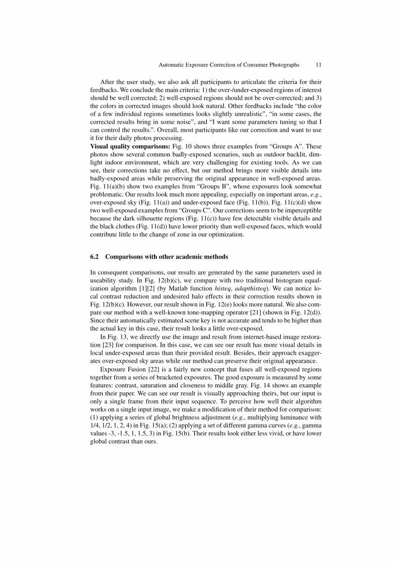
Fig. 16. Comparisons with learning-based tonal adjustment [4]. Images (a,b,d) are taken from [4].
We show the comparison with learning-based adjustment [4] and assisted correc-tion by expert in Fig. 16. As we can see, our result has more luminance details thantheir result on under-exposed areas and even much closer to the assisted result (from“Retoucher E” mentioned in [4]). Here, please ignore the difference in colors and fo-cus on the luminance modification since the assisted adjustment includes both exposurecorrection and white balance. Without the need of training images, our approach obtainappealing results as well.
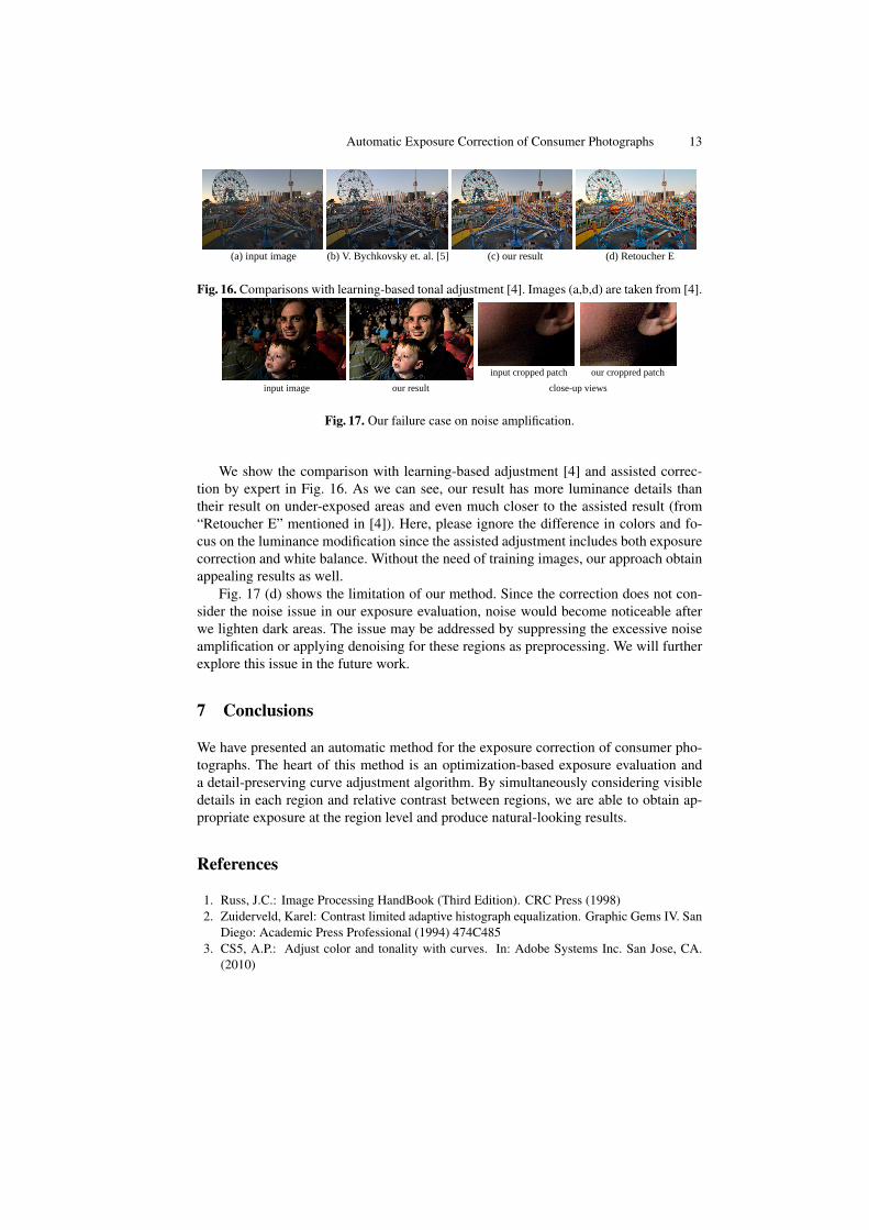
Fig. 17 (d) shows the limitation of our method. Since the correction does not con-sider the noise issue in our exposure evaluation, noise would become noticeable afterwe lighten dark areas. The issue may be addressed by suppressing the excessive noiseamplification or applying denoising for these regions as preprocessing. We will furtherexplore this issue in the future work.
7 Conclusions
We have presented an automatic method for the exposure correction of consumer pho-tographs. The heart of this method is an optimization-based exposure evaluation anda detail-preserving curve adjustment algorithm. By simultaneously considering visibledetails in each region and relative contrast between regions, we are able to obtain ap-propriate exposure at the region level and produce natural-looking results.
Diego: Academic Press Professional (1994) 474C4853. CS5, A.P.: Adjust color and tonality with curves. In: Adobe Systems Inc. San Jose, CA.
(2010)
14 Automatic Exposure Correction of Consumer Photographs
4. Bychkovsky, V., Paris, S., Chan, E., Durand, F.: Learning photographic global tonal adjust-ments with a database of input / output image pairs. CVPR (2011)
5. Ansel, A.: The Negative. The Ansel Adams Photography Series (1981)6. Battiato, S., Bosco, A., Castorina, A., Messina, G.: Automatic image enhancement by con-
tent dependent exposure correction. Journal on Applied Signal Processing 12 (2004) 1849–1860
7. Bhukhanwala, S.A., Ramabadran, T.V.: Automated global enhancement of digitized pho-tographs. IEEE Trans. on. Consumer Electronics 40 (1994) 1–10
8. dong Lee, K., Kim, S., Kim, S.D.: Dynamic range compression based on statistical analysis.ICIP (2009)
9. Kang, S.B., Kapoor, A., Lischinski, D.: Personalization of image enhancement. CVPR(2010)
10. Sobol, R.: Improving the retinex algorithm for rendering wide dynamic range photographs.Journal of Electronic Imaging 13, No. 1 (2004)
11. Chesnokov, V.: Dynamic range compression preserving local image contrast. In: GB Patent2417381. (2006)
12. Jobson, D.J., Rahman, Z., Woodell, G.A.: Properties and performance of a center/surroundretinex. IEEE Trans. on Image Processing 6 (1997) 451–462
13. Nayar, S.K., Branzoi, V.: Adaptive dynamic range imaging: Optical control of pixel expo-sures over space and time. (ICCV 2003)
14. Shimizu, S., Kondo, T., Kohashi, T., Tsuruta, M., Komuro, T.: A new algorithm of exposurecontrol based on fuzzy logic for video cameras. ICCE. (1992)
15. Yang, M., Wu, Y., Crenshaw, J., Augustine, B., Mareachen, R.: Face detection for automaticexposure control in handheld camera. In: ICVS. (2006)
16. Ilstrup, D., R, M.: One-shot optimal exposure control. In: ECCV. (2010)17. Brajovic, V.: Brightness perception, dynamic range and noise: a unifying model for adaptive
image sensors. In: CVPR. (2004)18. Safonov, I.: Automatic correction of amateur photos damaged by backlighting. GraphiCon
(2006)19. Mukherjee, J., Mitra, S.K.: Enhancement of color images by scaling the dct coefficients.
IEEE Trans. on Image Processing 17 (2008) 1783–179420. Ovsiannikov, I.: Backlit subject detection in an image. In: US Patent 7813545. (2010)21. Reinhard, E., Stark, M., Shirley, P., Ferwerda, J.: Photographic tone reproduction for digital