Automatic fault surface detection by using 3D Hough transformZhen Wang∗ and Ghassan AlRegib,Center for Energy & Geo Processing (CeGP), Georgia Institute of Technology
SUMMARY
Detection of faults plays an important role in the characteri-zation of reservoir regions. In this paper, we propose an auto-matic fault surface detection method using 3D Hough transfor-m to improve the interpretation efficiency. We first highlightthe likely fault points in seismic data by thresholding the cor-responding discontinuity volumes. Then, we apply 3D Houghtransform to detect the likely fault planes in seismic volumes.After filtering out the noisy planes, we apply the weightedplane fitting method to extract the smooth fault surfaces fromthe remaining fault planes. Experimental results show that theproposed method has the capability of detecting fault surfacesin real seismic data with high accuracy and fewer human inter-ventions.
INTRODUCTION
Conventionally, it is the experienced interpreters that manu-ally perform fault interpretation. However, with the giganticamount of seismic data collected in today’s hydrocarbon ex-ploration, manual interpretation is time consuming and laborintensive. Therefore, to improve the interpretation efficiency,in recent years several research teams have developed semi-automatic fault interpretation technologies that require limitedhuman interaction.
Most algorithms that were developed to semi-automaticallydetect faults in seismic volumes consist of two major steps.The first step is the selection of appropriate and useful seis-mic attributes. Since faults are the discontinuous regions a-long horizons, seismic attributes, including coherency (Mar-furt et al. (1999)), variance (Van Bemmel and Pepper (2000)),curvature (Boe and Daber (2010)), and gradient (Song et al.(2012)), have been proposed to characterize the geological struc-tures of faults. Interpreters apply thresholds on one or com-bined fault-sensitive seismic attributes to highlight the likelyfault points.
The second step is the extraction of fault structures from thesehighlighted fault points. Based on the dimensional disparity inseismic data, the detection methods are usually classified in-to two classes. One class of methods focuses on the detectionof fault lines in 2D seismic images and the other class detectsfault planes in 3D seismic volumes. AlBinHassan and Mar-furt (2003) suggested to detect fault lines in seismic sectionsby using 2D Hough transform. However, the detected resultsare not accurate enough because of noisy lines. To improve ac-curacy, Wang and AlRegib (2014b) filtered out the noisy linefeatures detected by 2D Hough transform based on the criteri-a derived from the geological constraints. Similarly, Admasuet al. (2006) applied the log-Gabor filter to remove noise a-
long directions of faults and tracked the fault lines through theneighboring seismic sections by fitting active contours. An-other fault tracking algorithm proposed by Wang and AlRegib(2014a) borrowed the ideas of motion vectors in video cod-ing and processing techniques and synthesized the fault linesby combining two reference fault lines. In contrast, Yan et al.(2012) implemented the ant colony algorithm to track faults inseismic sections.
In general, by tweaking local parameters, faults delineated in2D seismic images are more accurate than the detected faultsurfaces in 3D seismic volumes. Nevertheless, this processdoes not scale up when the size of the data set grows consid-erably and thus the algorithm’s efficiency degrades. Besides,without involving the coherence between neighboring section-s, the fault surfaces generated by connecting the detected re-sults in 2D sections are not accurate enough to reflect the 3Dcomplicated structures of faults.
To label fault surfaces in 3D seismic data, Gibson et al. (2005)proposed a multi-stage work flow. After highlighting the faultpoints in semblance cubes, they grouped them into the lo-cal planar patches and then merged these patches into largerfault surfaces under certain geometric constraints. However, itmakes this method inefficient that a group of parameters haveto be decided by trial and error. This issue was addressed inthe work of Cohen et al. (2006) where 3D directional filtersare applied on seismic volumes to enhance the semblance at-tribute and consequently a thinning algorithm extracts the one-pixel-width fault surfaces. The cascade Hough transform hasalso been introduced by Jacquemin and Mallet (2005) to detec-t fault surfaces. Similarly, Aqrawi and Boe (2011) suggestedto extract fault surfaces based on gradients calculated by 3DSobel filter while Hale (2013) proposed to first detect the 2Dfault lines in cross-sections of seismic volumes on different di-rections and then applied dynamic time warping to generatethe fault surfaces based on the boundary constraints derivedfrom the detected fault lines.
In this paper, we propose the automatic fault surface detectionmethod by using 3D Hough transform, which involves lim-ited human interventions. We first highlight the likely faultpoints in seismic volumes by thresholding the correspondingdiscontinuity volumes. Then, we apply 3D Hough transformon the binary volumes to detect the potential fault planes inseismic volumes. According to the likely positions and direc-tions of fault planes estimated by interpreters, we filter out thenoisy planes and obtain a group of fault planes located aroundthe fault regions. Since these planes are determined by thehighlighted fault points, we propose the weighted plane fittingmethod to extract local fault surfaces piecewise on depth direc-tion by involving the geological constraints. After connectingthe local fitted results, we obtain the smooth fault surfaces inseismic volumes.
The block diagram of the proposed method is shown in Fig-ure 1. In the following sections, we explain each step of theproposed method in detail.
Fault PointHighlighting
3D Hough Transform
Fault Surface Labeling
SeismicVolumes
Faultsurfaces
Figure 1: Block diagram of the proposed method.
Fault Point HighlightingThe most prominent feature of faults is the discontinuity inhorizons. Semblance attribute proposed by Marfurt et al. (1998)characterizes such discontinuity by involving neighboring in-formation and structural dips. In this paper, we propose thediscontinuity attribute as a logarithmic function of semblanceattribute in order to increase the contrast between fault re-gions and horizons. In 3D seismic data, x, y and z represen-t the inline, crossline, and depth direction, respectively. Fora point located at [x,y,z], we calculate its discontinuity val-ue D[x,y,z] in the corresponding analysis cube with an edgelength of (2rd +1), as shown in Eq. (1),
D[x,y,z] =
∣∣∣∣∣∣∣∣ln
⎡⎢⎢⎣
rd∑k=−rd
(rd∑
i, j=−rd
s[x+i,y+ j,z+k+Δz]
)2
(2rd+1)2rd∑
i, j,k=−rd
s2[x+i,y+ j,z+k+Δz]
⎤⎥⎥⎦∣∣∣∣∣∣∣∣, (1)
where s[x,y,z] represents seismic signal’s intensity at point [x,y,z]and rd decides the dimension of analysis cubes. Δz reflects theinfluence of structural dips on depth direction and is calculatedas follows,
Δz =⌊tanθx · i+ tanθy · j
⌉, (2)
where θx and θy respectively correspond to the dips along in-line and crossline direction and the function �·� rounds Δz tothe nearest integer. In Eq. (1), greater discontinuity value in-dicates that the point [x,y,z] has a higher possibility of beinglocated at fault regions. In contrast, the discontinuity valueclose to 0 means the point is in a horizon. To highlight thelikely fault points, we apply a global threshold on the obtaineddiscontinuity volume as follows,
B[x,y,z] =
{1 D[x,y,z]≥ D0
0 otherwise, (3)
where D0 as a designed parameter is determined empirically.Based on these highlighted fault points, we propose to extractfault planes by using 3D Hough transform in the followingsections.
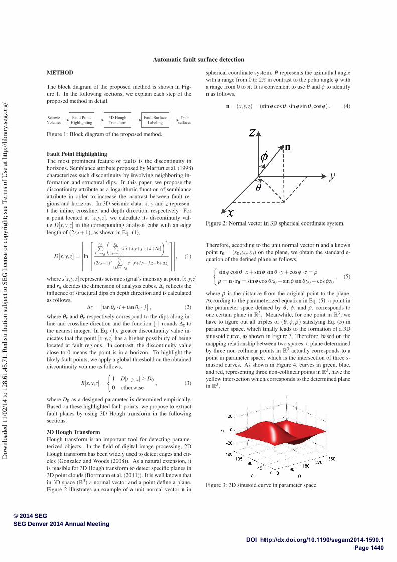
3D Hough TransformHough transform is an important tool for detecting parame-terized objects. In the field of digital image processing, 2DHough transform has been widely used to detect edges and cir-cles (Gonzalez and Woods (2008)). As a natural extension, itis feasible for 3D Hough transform to detect specific planes in3D point clouds (Borrmann et al. (2011)). It is well known thatin 3D space (R3) a normal vector and a point define a plane.Figure 2 illustrates an example of a unit normal vector n in
spherical coordinate system. θ represents the azimuthal anglewith a range from 0 to 2π in contrast to the polar angle φ witha range from 0 to π . It is convenient to use θ and φ to identifyn as follows,
n = (x,y,z) = (sinφ cosθ ,sinφ sinθ ,cosφ) . (4)
Figure 2: Normal vector in 3D spherical coordinate system.
Therefore, according to the unit normal vector n and a knownpoint r0 = (x0,y0,z0) on the plane, we obtain the standard e-quation of the defined plane as follows,{
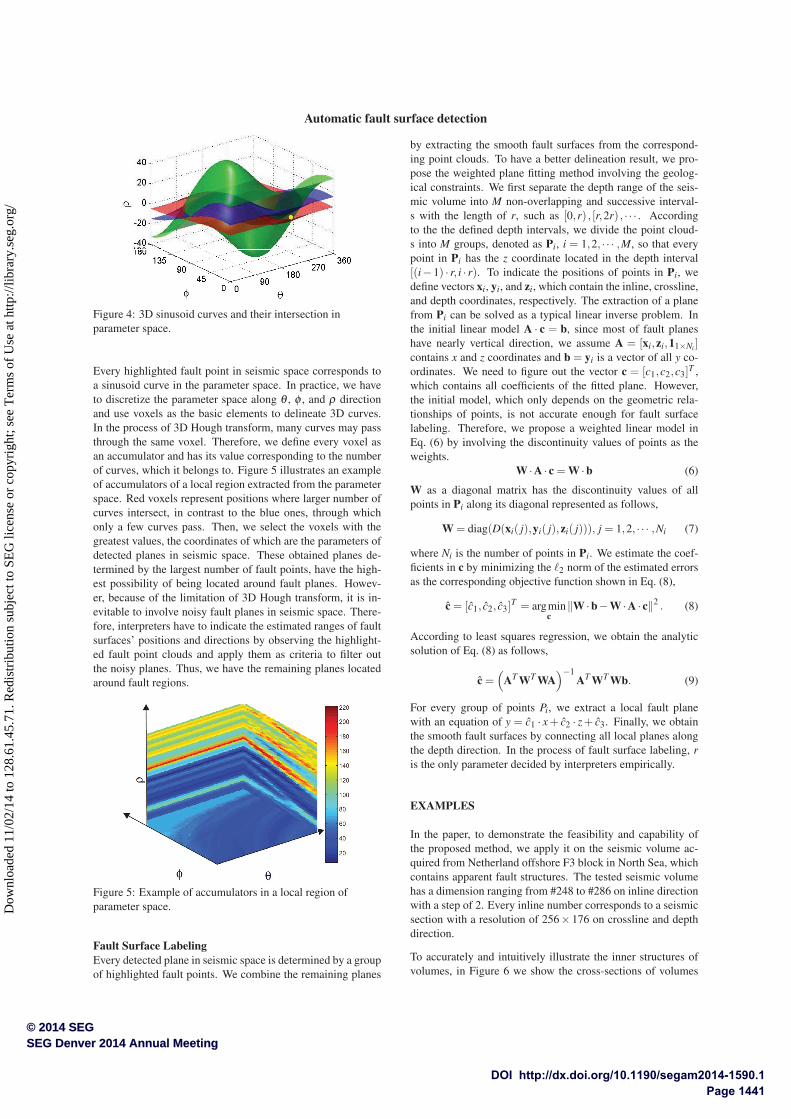
where ρ is the distance from the original point to the plane.According to the parameterized equation in Eq. (5), a point inthe parameter space defined by θ , φ , and ρ , corresponds toone certain plane in R
3. Meanwhile, for one point in R3, we
have to figure out all triples of (θ ,φ ,ρ) satisfying Eq. (5) inparameter space, which finally leads to the formation of a 3Dsinusoid curve, as shown in Figure 3. Therefore, based on themapping relationship between two spaces, a plane determinedby three non-collinear points in R
3 actually corresponds to apoint in parameter space, which is the intersection of three s-inusoid curves. As shown in Figure 4, curves in green, blue,and red, representing three non-collinear points in R
3, have theyellow intersection which corresponds to the determined planein R
Figure 4: 3D sinusoid curves and their intersection inparameter space.
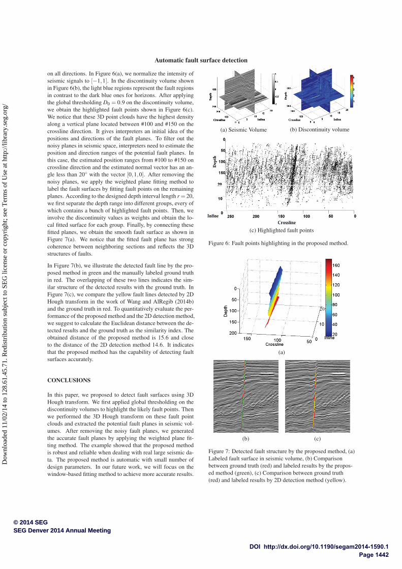
Every highlighted fault point in seismic space corresponds toa sinusoid curve in the parameter space. In practice, we haveto discretize the parameter space along θ , φ , and ρ directionand use voxels as the basic elements to delineate 3D curves.In the process of 3D Hough transform, many curves may passthrough the same voxel. Therefore, we define every voxel asan accumulator and has its value corresponding to the numberof curves, which it belongs to. Figure 5 illustrates an exampleof accumulators of a local region extracted from the parameterspace. Red voxels represent positions where larger number ofcurves intersect, in contrast to the blue ones, through whichonly a few curves pass. Then, we select the voxels with thegreatest values, the coordinates of which are the parameters ofdetected planes in seismic space. These obtained planes de-termined by the largest number of fault points, have the high-est possibility of being located around fault planes. Howev-er, because of the limitation of 3D Hough transform, it is in-evitable to involve noisy fault planes in seismic space. There-fore, interpreters have to indicate the estimated ranges of faultsurfaces’ positions and directions by observing the highlight-ed fault point clouds and apply them as criteria to filter outthe noisy planes. Thus, we have the remaining planes locatedaround fault regions.
Figure 5: Example of accumulators in a local region ofparameter space.
Fault Surface LabelingEvery detected plane in seismic space is determined by a groupof highlighted fault points. We combine the remaining planes
by extracting the smooth fault surfaces from the correspond-ing point clouds. To have a better delineation result, we pro-pose the weighted plane fitting method involving the geolog-ical constraints. We first separate the depth range of the seis-mic volume into M non-overlapping and successive interval-s with the length of r, such as [0,r) , [r,2r) , · · · . Accordingto the the defined depth intervals, we divide the point cloud-s into M groups, denoted as Pi, i = 1,2, · · · ,M, so that everypoint in Pi has the z coordinate located in the depth interval[(i−1) · r, i · r). To indicate the positions of points in Pi, wedefine vectors xi, yi, and zi, which contain the inline, crossline,and depth coordinates, respectively. The extraction of a planefrom Pi can be solved as a typical linear inverse problem. Inthe initial linear model A · c = b, since most of fault planeshave nearly vertical direction, we assume A = [xi,zi,11×Ni ]contains x and z coordinates and b = yi is a vector of all y co-ordinates. We need to figure out the vector c = [c1,c2,c3]
T ,which contains all coefficients of the fitted plane. However,the initial model, which only depends on the geometric rela-tionships of points, is not accurate enough for fault surfacelabeling. Therefore, we propose a weighted linear model inEq. (6) by involving the discontinuity values of points as theweights.
W ·A · c = W ·b (6)
W as a diagonal matrix has the discontinuity values of allpoints in Pi along its diagonal represented as follows,
where Ni is the number of points in Pi. We estimate the coef-ficients in c by minimizing the �2 norm of the estimated errorsas the corresponding objective function shown in Eq. (8),
c = [c1, c2, c3]T = argmin
c‖W ·b−W ·A · c‖2 . (8)
According to least squares regression, we obtain the analyticsolution of Eq. (8) as follows,
c =(
AT WT WA)−1
AT WT Wb. (9)
For every group of points Pi, we extract a local fault planewith an equation of y = c1 · x+ c2 · z+ c3. Finally, we obtainthe smooth fault surfaces by connecting all local planes alongthe depth direction. In the process of fault surface labeling, ris the only parameter decided by interpreters empirically.
EXAMPLES
In the paper, to demonstrate the feasibility and capability ofthe proposed method, we apply it on the seismic volume ac-quired from Netherland offshore F3 block in North Sea, whichcontains apparent fault structures. The tested seismic volumehas a dimension ranging from #248 to #286 on inline directionwith a step of 2. Every inline number corresponds to a seismicsection with a resolution of 256× 176 on crossline and depthdirection.
To accurately and intuitively illustrate the inner structures ofvolumes, in Figure 6 we show the cross-sections of volumes
on all directions. In Figure 6(a), we normalize the intensity ofseismic signals to [−1,1]. In the discontinuity volume shownin Figure 6(b), the light blue regions represent the fault regionsin contrast to the dark blue ones for horizons. After applyingthe global thresholding D0 = 0.9 on the discontinuity volume,we obtain the highlighted fault points shown in Figure 6(c).We notice that these 3D point clouds have the highest densityalong a vertical plane located between #100 and #150 on thecrossline direction. It gives interpreters an initial idea of thepositions and directions of the fault planes. To filter out thenoisy planes in seismic space, interpreters need to estimate theposition and direction ranges of the potential fault planes. Inthis case, the estimated position ranges from #100 to #150 oncrossline direction and the estimated normal vector has an an-gle less than 20◦ with the vector [0,1,0]. After removing thenoisy planes, we apply the weighted plane fitting method tolabel the fault surfaces by fitting fault points on the remainingplanes. According to the designed depth interval length r = 20,we first separate the depth range into different groups, every ofwhich contains a bunch of highlighted fault points. Then, weinvolve the discontinuity values as weights and obtain the lo-cal fitted surface for each group. Finally, by connecting thesefitted planes, we obtain the smooth fault surface as shown inFigure 7(a). We notice that the fitted fault plane has strongcoherence between neighboring sections and reflects the 3Dstructures of faults.
In Figure 7(b), we illustrate the detected fault line by the pro-posed method in green and the manually labeled ground truthin red. The overlapping of these two lines indicates the sim-ilar structure of the detected results with the ground truth. InFigure 7(c), we compare the yellow fault lines detected by 2DHough transform in the work of Wang and AlRegib (2014b)and the ground truth in red. To quantitatively evaluate the per-formance of the proposed method and the 2D detection method,we suggest to calculate the Euclidean distance between the de-tected results and the ground truth as the similarity index. Theobtained distance of the proposed method is 15.6 and closeto the distance of the 2D detection method 14.6. It indicatesthat the proposed method has the capability of detecting faultsurfaces accurately.
CONCLUSIONS
In this paper, we proposed to detect fault surfaces using 3DHough transform. We first applied global thresholding on thediscontinuity volumes to highlight the likely fault points. Thenwe performed the 3D Hough transform on these fault pointclouds and extracted the potential fault planes in seismic vol-umes. After removing the noisy fault planes, we generatedthe accurate fault planes by applying the weighted plane fit-ting method. The example showed that the proposed methodis robust and reliable when dealing with real large seismic da-ta. The proposed method is automatic with small number ofdesign parameters. In our future work, we will focus on thewindow-based fitting method to achieve more accurate results.
(a) Seismic Volume (b) Discontinuity volume
(c) Highlighted fault points
Figure 6: Fault points highlighting in the proposed method.
20
(a)
(b) (c)
Figure 7: Detected fault structure by the proposed method, (a)Labeled fault surface in seismic volume, (b) Comparisonbetween ground truth (red) and labeled results by the propos-ed method (green), (c) Comparison between ground truth(red) and labeled results by 2D detection method (yellow).
http://dx.doi.org/10.1190/segam2014-1590.1 EDITED REFERENCES Note: This reference list is a copy-edited version of the reference list submitted by the author. Reference lists for the 2014 SEG Technical Program Expanded Abstracts have been copy edited so that references provided with the online metadata for each paper will achieve a high degree of linking to cited sources that appear on the Web. REFERENCES
Admasu, F., S. Back, and K. Toennies, 2006, Auto-tracking of faults on 3D seismic data: Geophysics, 71, no. 6, A49–A53, http://dx.doi.org/10.1190/1.2358399.
AlBinHassan, N. M., and K. J. Marfurt, 2003, Fault detection using Hough transforms: Presented at the 83rd Annual International Meeting, SEG.
Aqrawi, A. A., and T. H. Boe, 2011, Improved fault segmentation using a dip guided and modified 3D Sobel filter: 81st Annual International Meeting, SEG, Expanded Abstracts, 999–1003.
Boe, T. H., and R. H. Daber, 2010, Seismic features and the human eye: RGB blending of azimuthal curvatures for enhancement of fault and fracture interpretation: Presented at the 80th Annual International Meeting, SEG.
Borrmann, D., J. Elseberg, K. Lingemann, and A. Nüchter, 2011, The 3D Hough transform for plane detection in point clouds: A review and a new accumulator design: 3D Research, 2, 1–13.
Cohen, I., N. Coult , and A. A. Vassiliou, 2006, Detection and extraction of fault surfaces in 3D seismic data: Geophysics, 71, no. 4, P21–P27, http://dx.doi.org/10.1190/1.2215357.
Gibson, D., M. Spann, J. Turner, and T. Wright, 2005, Fault surface detection in 3D seismic data: Geoscience and Remote Sensing: IEEE Transactions on, 43, 2094–2102.
Gonzalez, R. C., and R. E. Woods, 2008, Digital image processing: Prentice Hall.
Hale, D., 2013, Methods to compute fault images, extract fault surfaces, and estimate fault throws from 3D seismic images: Geophysics, 78, no. 2, O33–O43, http://dx.doi.org/10.1190/geo2012-0331.1.
Jacquemin, P., and J. Mallet, 2005, Automatic faults extraction using double Hough transform: 75th Annual International Meeting, SEG, Expanded Abstracts, 755–758.
Marfurt, K. J., R. L. Kirlin, S. L. Farmer, and M. S. Bahorich, 1998, 3D seismic attributes using a semblance-based coherency algorithm: Geophysics, 63, 1150–1165, http://dx.doi.org/10.1190/1.1444415.
Marfurt, K. J., V. Sudhaker, A. Gersztenkorn, K. D. Crawford, and S. E. Nissen, 1999, Coherency calculations in the presence of structural dip : Geophysics, 64, 104–111, http://dx.doi.org/10.1190/1.1444508.
Song, J., X. Mu, Z. Li, C. Wang, and S. Y., 2012, A faults identification method using dip guided facet model edge detector: 82nd Annual International Meeting, SEG, Expanded Abstracts, doi: 10.1190/segam2012-0042.1.
Van Bemmel, P. P., and R. E. F. Pepper, 2000, Seismic signal processing method and apparatus for generating a cube of variance values: U. S. Patent 6,151,555.
Wang, Z., and G. AlRegib , 2014a, Automatic fault tracking across seismic volumes via tracking vectors: IEEE ICIP.