162
Automatic segmentation and registration of CT and US images of abdominal aortic aneurysm using ITK Bjørn Hanch Sollie

Automatic segmentation and registration ofCT and US images of
abdominal aortic aneurysmusing ITK
Bjørn Hanch Sollie


NTNU Faculty of Information Technology,Norwegian University of Mathematics and Electrical EngineeringScience and Technology
DIPLOMA THESIS
FACULTY OF INFORMATION TECHNOLOGY,MATHEMATICS AND ELECTRICAL ENGINEERING
NTNU
Candidate: Stud.Techn. Bjørn Hanch Sollie
Discipline: Mathematics
Date started: February 26, 2002
Date due: July 23, 2002
New date due: August 20, 2002
Title: Automatic segmentation and registration of CT and USimages of abdominal aortic aneurysm using ITK
Thesis formulation: The thesis is about automatic segmentation and registra-tion of abdominal aortic aneurysm (AAA) as seen in postoperative CT images,using the Insight segmentation and registration toolkit (ITK). The focus should beset primarily on the segmentation. With this background, the thesis is expected tocontain:
• Theoretical background for the employed segmentation algorithm.
• Theoretical background for the employed registration algorithm.
• Segmentation of AAA as seen in postoperative CT images.
• Registration of postoperative CT and US images of AAA.
• Evaluation of the usefulness of ITK for solving these problems.
The diploma thesis is to be carried out at the Department of mathematical sciencesunder the supervision of Ketil Bø and Harald Hanche-Olsen, in cooperation withSintef Unimed under supervision of Frank Lindseth and Jon Harald Kaspersen.
Trond DigernesChair
Dept. of Mathematical Sciences
Harald Hanche-OlsenAssociate Professor
Dept. of Mathematical Sciences


Preface
This diploma thesis was written at the Faculty of Information Technology, Math-ematics and Electrical Engineering for the dept. of Mathematical Sciences at theNorwegian University of Science and Technology (NTNU). The thesis was donein cooperation with Sintef Unimed, which is part of Sintef, The Foundation forScientific and Industrial Research. The Sintef group is the largest independentresearch organization in Scandinavia.
The author of this thesis is Bjørn Hanch Sollie. Supervisor from the dept. ofComputer and Information Science was Associate Professor Ketil Bø. Supervisorfrom the dept. of Mathematical Sciences was Associate Professor Harald Hanche-Olsen. External supervisors at Sintef Unimed were Frank Lindseth and Jon HaraldKaspersen.
I started the work on this thesis with no prior knowledge of image processing ormedicine in general or medical imaging in particular. This work has been veryexploratory in the sense that none of my supervisors or I had any prior experiencewith the in-development medical imaging tool used, the Insight Segmentation andRegistration Toolkit (ITK). The ability to learn and use known and unknown ele-ments from the sciences of mathematics, programming, medicine and image pro-cessing, has been essential. Additionally, achieving a firm grasp of both the basicsand some more complex components of medical imaging from the bottom up, hasalso required a lot of learning. In hindsight I can safely say that it has been both afun and rewarding experience.
Lastly, the way I got involved with this work is a matter of funny and bizarrecoincidence, so much as to be worth mentioning here: When the time came tostart the work on my diploma thesis I still hadn’t managed to decide what I wantedto work with, despite a considerable search. Time continued to pass by, and bylate fall last year the issue of finding an appealing topic was starting to becomea matter of worrisome inconvenience. This was underlined by the fact that all Ireally knew about what I wanted to do was that it preferably include some practical

and immediately useful work. Then, one evening, when I was flipping through thechannels on my TV, and this very matter was occupying my mind, there was oneprogram on that caught my attention. It was a report about Sintef Unimed andtheir recent innovations and work in the field of medical imaging. Here was thepotential for something to do which was both practical, interesting and usefuland which could possibly even carry the reward of being fun. I jotted down afew names, as they appeared in the interviews on the TV screen. The next day Icontacted the people at Sintef Unimed with the hopes of appointing a meeting onthe matter, the eventual result of which is described on the next one hundred or sopages.
Trondheim, August 20, 2002
Bjørn Hanch Sollie

Abstract
The goal of this project was to perform automatic segmentation and registrationof the inner and outer aortic wall in abdominal aortic aneurysm as seen in post-operative CT and US images. These tasks were performed by using the existingframework provided by the Insight segmentation and registration toolkit (ITK),a new in-development software toolkit for performing segmentation and registra-tion. An evaluation is to be provided of the current usefulness of ITK to performthe cited tasks.
The methods explored for segmentation include use of the watershed algorithm,fuzzy connectedness and level sets, while for registration, the use of mutual infor-mation was investigated.
The achieved results are mixed. A scheme to perform segmentation of the innerand outer aortic walls with minimal user intervention has been presented. Thesegmentation is performed automatically after manual selection of only four initialvalues. The spatial extent of the segmented structure includes a region from belowthe renal arteries to the top of the iliac arteries, below the aortic bifurcation pointin the lower abdomen. Searches indicate that no such scheme has previously beenpresented. The use of watershed and fuzzy connectedness algorithms respectivelyare also discussed. Using using mutual information to automatically register CTand US images, with the use of two different image alignment optimizers, did notproduce satisfactory results.
The achieved results of the segmentation indicate that ITK is a medical imagingtool with great potential. The achieved results of the registration indicate that it isa bit too early to make full use of the toolkit in clinical applications. The currentlimitations of the ITK framework are thought to have been met for both of ourspecific problems, and thus the goals of the project were achieved.


Acknowledgements
Special thanks to the friendly staff at Sintef Unimed for offering me this work.
Special thanks to Frank Lindseth, Jon Harald Kaspersen, Ketil Bø and HaraldHanche-Olsen for all the help and assistance they have provided.
Thanks to Luis Ibanez, Joshua Cates and the other members of the insight-usersmailing list for patiently and thoroughly answering my questions on several occa-sions.
Thanks to Bjørn Olstad for help and advice prior to starting this work.
Thanks to Sven Loncaric and Marko Subasic for sharing with me some of thedetails of their work presented in [LONCA-01].
Thanks to Marleen de Bruijne for providing me with an article ([BRUIN-02])about the most recent work by her research team at the Image Sciences Instituteat the University Medical Center in Utrecht in the Netherlands.
Thanks to Toril Nagelhus Hernes for reading and providing feedback on my re-port.
Thanks to everyone I forgot to mention.


Contents
1 Introduction 1
1.1 Motivation . . . . . . . . . . . . . . . . . . . . . . . . . . . . . . 1
1.2 Problem definition . . . . . . . . . . . . . . . . . . . . . . . . . 3
1.2.1 Background . . . . . . . . . . . . . . . . . . . . . . . . . 3
1.2.2 Segmentation of the CT images . . . . . . . . . . . . . . 3
1.2.3 Registration of the CT and US images . . . . . . . . . . . 3
1.2.4 Evaluation of ITK . . . . . . . . . . . . . . . . . . . . . 4
1.3 Abdominal Aortic Aneurysm (AAA) . . . . . . . . . . . . . . . . 4
1.3.1 Introduction to AAA . . . . . . . . . . . . . . . . . . . . 4
1.3.2 Repair surgery . . . . . . . . . . . . . . . . . . . . . . . 5
1.3.3 Detection and condition assessment . . . . . . . . . . . . 6
1.4 Computer tomography (CT) imaging . . . . . . . . . . . . . . . . 8
1.5 Ultrasound (US) imaging . . . . . . . . . . . . . . . . . . . . . . 10
1.6 Image segmentation . . . . . . . . . . . . . . . . . . . . . . . . . 11
1.6.1 General image segmentation . . . . . . . . . . . . . . . . 11
1.6.2 Image segmentation in medicine . . . . . . . . . . . . . . 12
1.7 Image registration . . . . . . . . . . . . . . . . . . . . . . . . . . 12
1.7.1 General image registration . . . . . . . . . . . . . . . . . 12
1.7.2 Image registration in medicine . . . . . . . . . . . . . . . 13

ii Contents
2 Previous work 15
2.1 Segmentation of abdominal aortic aneurysm . . . . . . . . . . . . 15
2.1.1 Background . . . . . . . . . . . . . . . . . . . . . . . . . 15
2.1.2 Vessel axis extraction and border estimationapproaches . . . . . . . . . . . . . . . . . . . . . . . . . 16
2.1.3 Neural network approaches . . . . . . . . . . . . . . . . . 16
2.1.4 Active shape model (ASM) approaches . . . . . . . . . . 16
2.1.5 Watershed-based approaches . . . . . . . . . . . . . . . . 17
2.1.6 Region growing approaches . . . . . . . . . . . . . . . . 17
2.1.7 Level set-based approaches . . . . . . . . . . . . . . . . . 18
2.2 Registration of CT and US images . . . . . . . . . . . . . . . . . 18
2.2.1 Background . . . . . . . . . . . . . . . . . . . . . . . . . 18
2.2.2 Gradient and intensity information approaches . . . . . . 18
2.2.3 Mutual information approaches . . . . . . . . . . . . . . 19
2.3 Summary . . . . . . . . . . . . . . . . . . . . . . . . . . . . . . 19
3 Materials and methods 21
3.1 Problem solving strategy . . . . . . . . . . . . . . . . . . . . . . 21
3.1.1 Segmentation . . . . . . . . . . . . . . . . . . . . . . . . 21
3.1.2 Registration . . . . . . . . . . . . . . . . . . . . . . . . . 23
3.2 Solution criteria . . . . . . . . . . . . . . . . . . . . . . . . . . . 24
3.3 Visualization . . . . . . . . . . . . . . . . . . . . . . . . . . . . 24
3.4 ITK . . . . . . . . . . . . . . . . . . . . . . . . . . . . . . . . . 25
3.4.1 Introduction to ITK . . . . . . . . . . . . . . . . . . . . . 25
3.4.2 Overview of the segmentation filters . . . . . . . . . . . . 27
3.4.3 Overview of the registration filters . . . . . . . . . . . . . 27
3.4.4 Documentation . . . . . . . . . . . . . . . . . . . . . . . 28
3.4.5 Getting started . . . . . . . . . . . . . . . . . . . . . . . 29

Contents iii
3.4.6 Using ITK . . . . . . . . . . . . . . . . . . . . . . . . . 29
3.5 Segmentation algorithms . . . . . . . . . . . . . . . . . . . . . . 30
3.5.1 Overview . . . . . . . . . . . . . . . . . . . . . . . . . . 30
3.5.2 Watershed . . . . . . . . . . . . . . . . . . . . . . . . . . 30
3.5.3 Fuzzy connectedness . . . . . . . . . . . . . . . . . . . . 31
3.5.4 Level set methods . . . . . . . . . . . . . . . . . . . . . . 32
3.5.4.1 Introduction to level sets . . . . . . . . . . . . . 32
3.5.4.2 Level sets vs. deformable models . . . . . . . . 32
3.5.4.3 Evolving interfaces . . . . . . . . . . . . . . . 33
3.5.4.4 Finding a level set representation . . . . . . . . 33
3.5.4.5 Selecting a speed function . . . . . . . . . . . . 37
3.5.4.6 Selecting a potential function . . . . . . . . . . 38
3.5.4.7 Improving the performance . . . . . . . . . . . 38
3.5.4.8 Fast marching . . . . . . . . . . . . . . . . . . 39
3.5.4.9 Narrow banding . . . . . . . . . . . . . . . . . 40
3.5.4.10 Benefits of using level sets in image processing 40
3.6 Registration algorithms . . . . . . . . . . . . . . . . . . . . . . . 41
3.6.1 Overview . . . . . . . . . . . . . . . . . . . . . . . . . . 41
3.6.2 Mutual information . . . . . . . . . . . . . . . . . . . . . 41
3.6.2.1 Introduction to mutual information . . . . . . . 41
3.6.2.2 Entropy . . . . . . . . . . . . . . . . . . . . . 42
3.6.2.3 Finding a transformation estimator . . . . . . . 42
3.6.2.4 Stochastic maximization of the mutual infor-mation . . . . . . . . . . . . . . . . . . . . . . 44
4 Experiments and results 47
4.1 Image data . . . . . . . . . . . . . . . . . . . . . . . . . . . . . . 47
4.1.1 CT image data . . . . . . . . . . . . . . . . . . . . . . . 47
iv Contents
4.1.2 US image data . . . . . . . . . . . . . . . . . . . . . . . 49
4.1.3 Initial registration . . . . . . . . . . . . . . . . . . . . . . 50
4.2 The watershed approach . . . . . . . . . . . . . . . . . . . . . . 51
4.2.1 The problems . . . . . . . . . . . . . . . . . . . . . . . . 51
4.2.2 Attempted corrections . . . . . . . . . . . . . . . . . . . 53
4.2.3 Conclusion . . . . . . . . . . . . . . . . . . . . . . . . . 53
4.3 The fuzzy connectedness approach . . . . . . . . . . . . . . . . . 53
4.3.1 The problems . . . . . . . . . . . . . . . . . . . . . . . . 53
4.3.2 Attempted corrections . . . . . . . . . . . . . . . . . . . 55
4.3.3 Conclusion . . . . . . . . . . . . . . . . . . . . . . . . . 55
4.4 Implementing level sets . . . . . . . . . . . . . . . . . . . . . . . 56
4.4.1 Background . . . . . . . . . . . . . . . . . . . . . . . . . 56
4.4.2 Manual initialization . . . . . . . . . . . . . . . . . . . . 56
4.4.3 Automatic lumen segmentation . . . . . . . . . . . . . . 58
4.4.4 Automatic thrombus segmentation . . . . . . . . . . . . . 58
4.4.5 3D segmentation of the lumen . . . . . . . . . . . . . . . 59
4.4.5.1 Overview . . . . . . . . . . . . . . . . . . . . 59
4.4.5.2 Preprocessing . . . . . . . . . . . . . . . . . . 59
4.4.5.3 Segmentation . . . . . . . . . . . . . . . . . . 65
4.4.5.4 Postprocessing . . . . . . . . . . . . . . . . . . 72
4.4.6 3D segmentation of the thrombus . . . . . . . . . . . . . 74
4.4.6.1 Overview . . . . . . . . . . . . . . . . . . . . 74
4.4.6.2 Preprocessing . . . . . . . . . . . . . . . . . . 74
4.4.6.3 Segmentation . . . . . . . . . . . . . . . . . . 79
4.4.6.4 Postprocessing . . . . . . . . . . . . . . . . . . 84
4.4.7 2D segmentation of the thrombus . . . . . . . . . . . . . 85
4.4.7.1 Overview . . . . . . . . . . . . . . . . . . . . 85

Contents v
4.4.7.2 Preprocessing . . . . . . . . . . . . . . . . . . 86
4.4.7.3 Segmentation . . . . . . . . . . . . . . . . . . 86
4.4.7.4 Postprocessing . . . . . . . . . . . . . . . . . . 90
4.4.7.5 The segmentation error . . . . . . . . . . . . . 91
4.5 Implementing mutual information optimization . . . . . . . . . . 94
4.5.1 Background . . . . . . . . . . . . . . . . . . . . . . . . . 94
4.5.2 The CT and US image modalities . . . . . . . . . . . . . 94
4.5.3 Registering CT and US images . . . . . . . . . . . . . . . 96
4.5.3.1 Manual preparations . . . . . . . . . . . . . . . 96
4.5.3.2 Full automatization . . . . . . . . . . . . . . . 97
4.5.4 The registration procedure . . . . . . . . . . . . . . . . . 98
4.5.5 Using the GradientDescent optimizer . . . . . . . . . . . 100
4.5.6 Using the RegularStepGradientDescent optimizer . . . . . 101
4.5.7 Parameter selection . . . . . . . . . . . . . . . . . . . . . 102
4.5.8 The problems . . . . . . . . . . . . . . . . . . . . . . . . 103
4.5.9 Attempted corrections . . . . . . . . . . . . . . . . . . . 103
5 Discussion and conclusions 105
5.1 Segmentation . . . . . . . . . . . . . . . . . . . . . . . . . . . . 105
5.2 Registration . . . . . . . . . . . . . . . . . . . . . . . . . . . . . 106
5.3 Conclusive evaluation of ITK . . . . . . . . . . . . . . . . . . . . 107
5.4 Conclusion . . . . . . . . . . . . . . . . . . . . . . . . . . . . . 108
6 Future work 111
6.1 Improving the segmentation scheme . . . . . . . . . . . . . . . . 111
6.2 Improving the registration . . . . . . . . . . . . . . . . . . . . . 112
6.3 Improving ITK . . . . . . . . . . . . . . . . . . . . . . . . . . . 112
6.4 Further development . . . . . . . . . . . . . . . . . . . . . . . . 113

vi Contents
A Tables and charts 115
A.1 Error measurements of the 3D lumensegmentation . . . . . . . . . . . . . . . . . . . . . . . . . . . . 115
A.2 Evolution of the lumen 3D segmentation . . . . . . . . . . . . . . 117
A.3 Error measurements of the 3D thrombussegmentation . . . . . . . . . . . . . . . . . . . . . . . . . . . . 120
A.4 Evolution of the thrombus 3D segmentation . . . . . . . . . . . . 121
A.5 Error measurements of the 2D thrombussegmentation . . . . . . . . . . . . . . . . . . . . . . . . . . . . 124
A.6 Evolution of the thrombus 2D segmentation . . . . . . . . . . . . 125
B Glossary 135
Bibliography 137

List of Figures
1.1 Abdominal aortic aneurysm. . . . . . . . . . . . . . . . . . . . . 4
1.2 Treatment of abdominal aortic aneurysm. To the left, a healthyaorta. In the middle, a diseased aorta prior to surgery. To theright, an aorta after endovascular surgery, repaired with a stent graft. 5
1.3 A stent graft for surgical repair of abdominal aortic aneurysm. . . 6
1.4 Examples of abdominal aortic aneurysms. The outer aortic wall(thrombus region) has been manually delimited by a solid whiteline. . . . . . . . . . . . . . . . . . . . . . . . . . . . . . . . . . 7
1.5 Example of a CT image. . . . . . . . . . . . . . . . . . . . . . . 8
1.6 Example of an ultrasound image. . . . . . . . . . . . . . . . . . . 10
3.1 CT and US images, registered with a marker and positioning sys-tem, displaying a similar anatomical region of the abdomen. . . . 24
3.2 Illustration of general filter operation in ITK. The input and outputare usually images, but may be other types of data objects as well.The input is usually the output of another filter. Similarly, theoutput is usually passed on to another filter. Connecting filterssequentially, the output data of one filter serves as the input datafor the next. . . . . . . . . . . . . . . . . . . . . . . . . . . . . . 29
3.3 Level set formulation of the equations of motion. The upper twoimages show the curveΓ and the surfaceΨ(x) att = 0. The lowertwo images show the curveΓ and the corresponding surfaceΨ(x)at timet. . . . . . . . . . . . . . . . . . . . . . . . . . . . . . . . 36
3.4 A narrow band of widthε around the level set. . . . . . . . . . . . 40

viii List of Figures
4.1 Two CT slices from the same volume showing the variation inintensities after conversion. Note especially the difference ingraylevel value of the lumen. In the left picture, the lumen is therelatively dark region with a brighter circle around it, while in theright picture, the same region is relatively bright overall, almostto the point of being solid. . . . . . . . . . . . . . . . . . . . . . 48
4.2 Two US slices from the same volume. In the left image, the bi-furcated stent graft can be vaguely seen slightly to the left in theimage. The dark region above it is caused by most of the sound-waves being reflected by the graft. In the right image, the graftcan can be seen as a small dark circular area within the aneurysm,which is the bigger and slightly brighter region around it. . . . . . 49
4.3 Examples of 3D watershed segmentation. The top left picture isthe initial slice while the other three are the same slice segmentedwith different sets of parameters as follows: Top right: threshold= 0.08, level = 0.07. Bottom left: threshold = 0.10, level = 0.07.Bottom right: threshold = 0.08, level = 0.03. By varying the pa-rameters only very slightly, significantly different segmentationsare obtained . . . . . . . . . . . . . . . . . . . . . . . . . . . . . 52
4.4 Example of 3D fuzzy connectedness segmentation. The right up-per and lower images are initial slices from the same volume. Theleft upper and lower images are the same slices, segmented us-ing the same set of parameters. This is a typical example of thealgorithm segmenting both too little and too much. . . . . . . . . 54
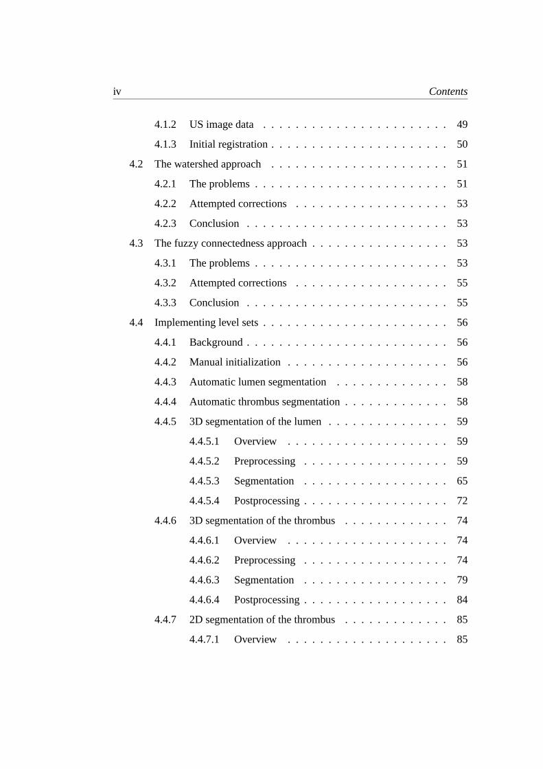
4.5 The four initial values selected through the manual initializationof the CT segmentation. . . . . . . . . . . . . . . . . . . . . . . . 57
4.6 Illustration of the desired results of the segmentation process. Tothe left, the region acquired by lumen segmentation. To the right,the region acquired by thrombus segmentation. . . . . . . . . . . 57
4.7 Two initial slices from the same unfiltered volume. In the leftslice, taken from below the bifurcation point, the lumen can beseen as two bright round regions next to each other in the middleof the picture. In the right slice, taken from above the bifurcationpoint, the lumen is seen as a single bright region. . . . . . . . . . 60
4.8 Gaussian filtered image, created with DiscreteGaussianImage-Filter (variance = 0.9). . . . . . . . . . . . . . . . . . . . . . . . 60

List of Figures ix
4.9 Median filtered image, created with MedianImageFilter(radius = 2). . . . . . . . . . . . . . . . . . . . . . . . . . . . . . 62
4.10 Contrast adjusted image (ilower = 70 andiupper = 170). . . . . . . 63
4.11 Gradient magnitude image, created with GradientMagnitudeIm-ageFilter. . . . . . . . . . . . . . . . . . . . . . . . . . . . . . . 64
4.12 Gradient image with optimized dynamic range, created withRescaleIntensityImageFilter (OutputMinimum = 0, OutputMax-imum = 255). . . . . . . . . . . . . . . . . . . . . . . . . . . . . 64
4.13 Pseudocode for the 3D level set segmentation of the lumen. . . . . 68
4.14 Slices from the 3D level set filtered image, created with ShapeDe-tectionLevelSetFilter. (The numerical parameters used are listedin table 4.1.) . . . . . . . . . . . . . . . . . . . . . . . . . . . . . 68
4.15 3D level set filtering of the lumen, showing the evolution of thesolution. From top left to bottom right, the images show the initialcubical level set and the segmented lumen region after 10, 20 and30 iterations. . . . . . . . . . . . . . . . . . . . . . . . . . . . . 70
4.16 3D level set filtering of the lumen, showing the evolution of thesolution. From top left to bottom right, the images show the seg-mented lumen region after 40, 50, 60 and 100 iterations. Thelower right image is also the final solution. . . . . . . . . . . . . . 71
4.17 Binary median filtered image, created with BinaryMedianImage-Filter (radius = 2). . . . . . . . . . . . . . . . . . . . . . . . . . . 72
4.18 Rendered model of the lumen region segmented using level setsin 3D. . . . . . . . . . . . . . . . . . . . . . . . . . . . . . . . . 73
4.19 Slices from the initial unfiltered image. . . . . . . . . . . . . . . . 74
4.20 Slices from the initial image after the segmented region has beenmasked. . . . . . . . . . . . . . . . . . . . . . . . . . . . . . . . 75
4.21 Intensity values aboveiupper = 170 have been thresholded off.Voxels with intensities above this limit have all been set toiupper. . 76
4.22 Gaussian filtered image, created with DiscreteGaussianImage-Filter (variance = 1.0). . . . . . . . . . . . . . . . . . . . . . . . 77
4.23 Median filtered image, created with MedianImageFilter(radius = 2). . . . . . . . . . . . . . . . . . . . . . . . . . . . . . 77

x List of Figures
4.24 Gradient magnitude image, created with GradientMagnitudeIm-ageFilter. . . . . . . . . . . . . . . . . . . . . . . . . . . . . . . 78
4.25 Gradient image with optimized dynamic range, created withRescaleIntensityImageFilter (OutputMinimum = 0, OutputMax-imum = 255). Note how different the edge features in these slicesare from those shown in figure 4.12, especially how the traces ofthe lumen have been removed and those of the thrombus are moreprominent. . . . . . . . . . . . . . . . . . . . . . . . . . . . . . . 78
4.26 Pseudocode for the 3D level set segmentation of the thrombus. . . 80
4.27 Slices from the 3D level set filtered image, created with ShapeDe-tectionImageFilter. (The numerical parameters used are listed intable 4.2.) . . . . . . . . . . . . . . . . . . . . . . . . . . . . . . 80
4.28 3D level set filtering of the thrombus, showing the evolution of thesolution. From top left to bottom right, the images show the initiallevel set and the segmented region after 10, 20 and 30 iterations.Notice that the initial level set is the same as the segmentationshown in figure 4.18 . . . . . . . . . . . . . . . . . . . . . . . . . 82
4.29 3D level set filtering of the thrombus, showing the evolution ofthe solution. From top left to bottom right, the images show thesegmented region after 40, 50, 70 and 90 iterations. The lowerright image shows the final segmentation. . . . . . . . . . . . . . 83
4.30 Binary median filtered image, created using the BinaryMedianIm-ageFilter (radius = 3). . . . . . . . . . . . . . . . . . . . . . . . . 84
4.31 Rendered model of the thrombus region segmented using levelsets in 3D. . . . . . . . . . . . . . . . . . . . . . . . . . . . . . . 85
4.32 Pseudocode for the 2D level set segmentation of the thrombus. . . 87
4.33 Slices from the 2D level set filtered image, created using theShapeDetectionImageFilter. (The numerical parameters used arelisted in table 4.3.) . . . . . . . . . . . . . . . . . . . . . . . . . 87
4.34 2D level set filtering, showing the evolution of the solution in oneof the slices. From top left to bottom right, the images show theinitial level set and the segmented region after 10, 30 and 60 iter-ations. The lower right image shows the final segmentation. . . . . 88

List of Figures xi
4.35 2D level set filtering, showing the evolution of the solution in an-other of the slices. From top left to bottom right, the images showthe segmented region after 10, 30 and 130 iterations. The lowerright image shows the final segmentation. . . . . . . . . . . . . . 89
4.36 Binary median filtered image, created with BinaryMedianImage-Filter (radius = 3). . . . . . . . . . . . . . . . . . . . . . . . . . . 90
4.37 Rendered model of the thrombus region segmented using levelsets in 2D. . . . . . . . . . . . . . . . . . . . . . . . . . . . . . . 91
4.38 Illustration of the positions of the five slices used to calculate thesegmentation error. . . . . . . . . . . . . . . . . . . . . . . . . . 92
4.39 Illustration of the error measures in slices 1-4, above the bifurca-tion point. . . . . . . . . . . . . . . . . . . . . . . . . . . . . . . 93
4.40 Illustration of the error measures in slice 5, below the bifurcationpoint. In this case, the segmentation error is measured separatelyfor both of the iliac arteries. . . . . . . . . . . . . . . . . . . . . . 93
4.41 CT and US images of similar features in the abdomen prior tomanual extraction of the subregions to be registered. The CT andUS images are from corresponding data sets. While the lumen andthe thrombus show up as solid regions in the CT images, it is theedges of these structures that are the most predominant features inthe US images. The lower right US image also illustrates how USdata is often very degraded by noise. . . . . . . . . . . . . . . . . 95
4.42 Pseudocode for the registration procedure. . . . . . . . . . . . . . 99
A.1 The chart shows the growth measure ratio for each check of thestopping criterion, performed every 10 iterations. Notice how itconverges almost asymptotically to 1. . . . . . . . . . . . . . . . 117
A.2 The chart shows the growth measure ratio for each check of thestopping criterion, performed every 10 iterations. . . . . . . . . . 121
A.3 The chart shows the total number of iterations per slice in each ofthe three data sets for the 2D thrombus segmentation. . . . . . . . 125


1 Introduction
In this chapter we present a brief introduction and explanation for some importantterms and concepts essential to understand and to solve the tasks at hand. Startingwith our motivations and definition of the problem, we continue by explaining thebasics of computer tomography (CT) and ultrasound (US) imaging, abdominalaortic aneurysm (AAA), image segmentation and image registration.
1.1 Motivation
The interest for segmentation and registration of medical images has greatly in-creased over the past decades. Our knowledge of the causes and treatment ofmedical conditions has increased by orders of magnitude. With the advancesin computer technology in general, and processing power and image acquisitiontechniques in particular, the amount of research in the field of medical imaginghas grown dramatically.
The introduction of x-ray computer tomography (CT) 25 years ago revolutionizedmedical imaging. CT provided the first clear cross sectional images of the humanbody with substantial contrast between different types of soft tissues. Since then,medical imaging has increasingly become a more important tool in all stages ofpatient treatment. Today, surgeons and radiologists commonly use complex visu-alization software to plan, simulate and monitor complicated surgery.
Image segmentation denotes the process of subdividing an image into its con-stituent parts or objects [RCEGW-93], while image registration denotes the pro-cess of bringing the involved pictures into spatial alignment [VIERG-97]. Animaging modality refers to a specific way of acquiring images, such as CT orultrasound (US) for example. Multimodal registration refers to registration ofimages acquired through different image acquisition techniques (such as CT andUS).

2 Introduction
Accurate and reproducible segmentation and registration schemes are becomingmore important in view of the rapid increase in the use of three-dimensional imag-ing modalities. An accurate segmentation allows for accurate quantitative andmorphological analysis and is indispensable for proper visualization and inter-pretation of images, for preoperative planning and for postoperative assessment.Manual segmentation and registration of, especially three-dimensional, imagesare time-consuming and hence expensive tasks. Manual segmentation is also sub-jective and thus cannot be reproduced, and often a high level of expertise is re-quired.
Minimally invasive endovascular surgery on the abdominal aorta and postopera-tive assessment after such surgery are areas in which the use of automation andmultimodal imaging is becoming a promising, realistic and viable possibility. Theabdominal aorta is a delicate and crucial part of the human body, and developingnew and effective procedures to reduce the risks of treatment is therefore essential.This is also true in the treatment of abdominal aortic aneurysm, a disease whichwill commonly lead to serious impairment or death, if left untreated.
CT is the primary tool for patient followup assessment today. By employing ultra-sound equipment instead, patients may be spared from going through up to severalCT sessions, thereby reducing health risks from x-ray radiation considerably, asultrasound equipment is non-radiating. In this context, development of an auto-matic segmentation and registration scheme for CT and US has the potential tocontribute to both safer and better treatment.
Software development is generally both time-consuming and costly. With the de-velopment of ITK, the Insight segmentation and registration toolkit, the medicalcommunity will receive a new tool, freely available to anyone, specifically de-signed for segmentation and registration of images in medical settings. ITK hasthe potential to make development of software for medical imaging applicationseasier, faster and more cost-effective. Its potential makes it well worth for themedical imaging communities to make use of the new software and assess howwell it performs for the specific need of each community; in this case segmenta-tion and registration of abdominal aortic aneurysm as seen in CT and US images.

Problem definition 3
1.2 Problem definition
1.2.1 Background
The tools used to implement the software are the C++ programming language andthe Insight segmentation and registration toolkit (ITK). As the central problemsare segmentation and registration, and not developing ITK, the focus has beenkept on using the ITK package as-is. Extra functionality was only implementedwhen strictly necessary, or when the time-cost of adding needed features was notcritical.
Although focusing strictly on either segmentation or registration would have beenpossible, there was agreement between all supervisors and the candidate from thebeginning that the study include both a segmentation problem and a registrationproblem. This choice was made to test and evaluate both of the two main branchesof functionality in ITK. The segmentation problem is presented in the most detail.
1.2.2 Segmentation of the CT images
We seek to extract the structures of the inner and outer aortic walls in postoperativeCT images of patients with abdominal aortic aneurysm. The extracted structuresshould contain all parts of the abnormally dilated aortic tissue and the inner andouter aortic wall in the height of the surgically inserted stent graft. Thus, thesegmented structures will represent the aorta from below the renal arteries to thetop of the iliac arteries, including the aortic bifurcation point. See figures 1.1 and1.2 for illustrations.
1.2.3 Registration of the CT and US images
We seek to register the postoperative CT images with postoperative followup USimages using rigid registration techniques only. Although the CT and US imagesare initially registered using a marker and positioning system, this initial registra-tion contains inaccuracies, and the objective is to improve it.

4 Introduction
1.2.4 Evaluation of ITK
A conclusive evaluation of the current usefulness of ITK for solving the segmen-tation and registration problems described is provided.
1.3 Abdominal Aortic Aneurysm (AAA)
1.3.1 Introduction to AAA
Abdominal aortic aneurysm (AAA) denotes the disease in which the infrarenalabdominal aorta tends to increase in size, either slowly or suddenly, resulting fromweakened arterial walls. Aneurysms may occur in any blood vessel in the body,but the most common place in the abdomen is on the aorta between the renalarteries and the aortic bifurcation point in the lower abdomen. An illustration ofthis can be seen in figure 1.1.
Figure 1.1: Abdominal aortic aneurysm.
An AAA is usually diagnosed when an increase of more than 50 % of the aorticdiameter is detected relative to a normal healthy diameter [RAVHO-98], or whenthe diameter is bigger than 50-55mm and increasing. Once present, AAAs maycontinue to enlarge and, if left untreated, become increasingly susceptible to rup-ture, usually resulting in lethal hemorrhage [MAGEE-00]. AAA is the 13th majorcause of death in the United States [BELKI-94], and occurs in up to seven percentof people of age 60 and older.

Abdominal Aortic Aneurysm (AAA) 5
1.3.2 Repair surgery
Worldwide, approximately 100,000 interventions for AAA repair are performedeach year, of which around 30 % are endovascular [ECALL-97]. An AAA ex-panding at a faster rate than 5mm over a period of six months is perceived to be ata high risk for imminent rupture, usually prompting surgical repair [BROWN-92].During the endovascular repair surgery, a synthetic stent graft is positioned insidethe aortic lumen to correct the blood flow and to reduce stress on the aortic walls.See figure 1.2 for an illustration.
Figure 1.2: Treatment of abdominal aortic aneurysm. To the left, a healthyaorta. In the middle, a diseased aorta prior to surgery. To the right, an aortaafter endovascular surgery, repaired with a stent graft.
Progressing aneurysmal disease after surgery and damage to or fatigue of the graftmaterial may result in leakage, curling, twisting and migration of the graft. Com-plications of this nature may eventually result in rupture or occlusion [BRUIN-01].As a consequence of this, careful and frequent patient followup is required. Apatient is imaged every three to twelve months, depending on the state of theaneurysm.
After surgery, the volume in the aneurysm between the graft and the aortic wallis usually filled with thrombus. In the remainder of this text, the outer aortic wallwill, for the sake of simplicity, often be referred to as the thrombus region, or justthe thrombus. Also, the inner aortic wall, which includes the stent graft and theregion inside the aorta with unobstructed blood flow, will regularly be referred toas the lumen region or just the lumen, unless otherwise noted.
The surgically inserted stent graft is made up of a woven polyester tube (usuallygore-tex) covered by a tubular metal mesh (usually stainless steel). An exampleof what such a graft may look like can be seen in figure 1.3.

6 Introduction
Figure 1.3: A stent graft for surgical repair of abdominal aortic aneurysm.
1.3.3 Detection and condition assessment
Ultrasound is the imaging modality most frequently used to determine if a pa-tient has an abdominal aortic aneurysm [BLANK-00]. The most widely usedmethod for further AAA planning and condition assessment is computer tomogra-phy (CT). Intravenous injection of contrast during CT image acquisition providesgood enhancement of the abdominal aorta.
The followup examination procedure usually includes some form of aneurysmdelimitation. As of today, this procedure is most commonly performed with somedegree of manual intervention. As previously mentioned, the problems with thisis that performing this task manually is time consuming, thus expensive, and it issubject to different radiologists producing different results.
To reduce analysis time, reduce variability and to increase reproducibility, auto-matic segmentation of the abdominal aorta and the aneurysm would be of greatvalue. Unfortunately, CT images of AAA are difficult to segment, because theouter aortic boundary is often obscured by surrounding tissue of similar density.There are also lot of other structures close in proximity to the aortic wall, whichwill frequently reduce the visibility of edges.
The radius of the aneurysm may also vary greatly over a short distance, and vari-ations in size and shape may be large between patients as well as in one patientover time. This can make the boundary difficult to detect even when surroundingstructures are absent. Lumen and thrombus texture and grayvalue can vary withthe presence of calcifications, graft metal, intravenous contrast and differencesbetween individual CT scanners.

Abdominal Aortic Aneurysm (AAA) 7
Figure 1.4: Examples of abdominal aortic aneurysms. The outer aortic wall(thrombus region) has been manually delimited by a solid white line.

8 Introduction
1.4 Computer tomography (CT) imaging
Computer tomography (CT), also referred to as computer assisted tomography(CAT), is a method of obtaining image data from different angles of differentparts of the body using x-rays. With the help of a computer, this information isprocessed to create a cross sectional view of body tissues and organs.
CT imaging is a powerful imaging tool because it can show several types of tissuesand materials, fluids, bone, blood vessels and internal organs with great claritycompared to most other imaging techniques. For this reason, CT is one of the besttools today for studying the abdomen. Using specialized equipment and expertiseto create and interpret CT scans of the body, radiologists can more easily diagnoseproblems such as cancers, infectious diseases, cardiovascular disease and, in ourcase, abdominal aortic aneurysm.
Figure 1.5: Example of a CT image.
CT imaging works by passing small controlled amounts of x-ray radiation throughthe body [RSNAW-02]. Different materials and tissues inside the body absorbvariable amounts of radiation, and the differences in the level of radiation emerg-ing on the other side is recorded by an array of detectors, which measure the x-rayprofile. This is in contrast to conventional x-ray radiology, where the x-rays pass-ing through the imaged object are instead captured on a special film.
A rotating gantry inside the CT scanner has an x-ray tube mounted on one sideand an arc-shaped detector on the opposite side. An x-ray beam is emitted in afan-shape as the x-ray tube and detector rotates around the patient. Each time thetube and detector makes one full rotation, the image of a thin section is acquired.

Computer tomography (CT) imaging 9
During each rotation, the detector records about 1,000 profiles of the expandedx-ray beam. Each profile is then reconstructed by a dedicated computer into a twodimensional cross-sectional image, or slice, of the section that was scanned.
When this is done multiple times in succession, while moving the patient’s bodya small distance relative to the frame for each time, the result is a set of multipleimages which may be assembled to give a detailed three-dimensional view of theinterior of the patient’s body.
Advantages:
• CT examinations are fast and simple and can quickly reveal internal injuriesand bleeding.
• CT imaging has been shown to be a cost-effective tool for a wide range ofclinical problems.
• CT imaging offers detailed views of many different kinds of tissues.
• CT imaging is painless, noninvasive and accurate.
• Through use of CT scanning, it is possible to identify both normal and abnor-mal structures. This makes it a useful tool for guiding radiotherapy, needlebiopsies and other minimally invasive procedures. In many cases this caneliminate the need for invasive surgery.
Disadvantages:
• CT involves exposure to radiation in the form of x-rays. The typical radia-tion dose from a CT exam is equivalent to the natural background radiationreceived over a year’s time. Special care must be taken during x-ray examina-tions and the patient’s abdomen and pelvis should normally be shielded by alead apron. In Norway alone, it is estimated that 40-50 patients develop fatalcancer every year, due to exposure to x-rays from CT scanners [TNRPA-02].
• CT exams are generally not recommended for pregnant women.
Limitations:
• Very fine details in soft tissue cannot always be seen with CT imaging. Insome situations, soft tissues may be obscured by bone structures. In thesecases, magnetic resonance (MR) imaging may be preferable.
• Using CT imaging as a means of guidance during patient surgery is inconve-nient, as the patient will have to be moved in and out of the CT scanner eachtime an updated image is needed.

10 Introduction
1.5 Ultrasound (US) imaging
Ultrasound (US) imaging, also referred to as sonography, is a method of obtainingimages of the inside of the body through the use of high frequency sound waves.Ultrasound imaging is based on the same principles involved in the sonar used fornavigation by ships at sea. As a controlled sound bounces against an object, theechoing waves can be used to identify how far away the object is, how big it is,and how uniform it is.
In preparation for the procedure, the skin of the area to be examined is exposedand coated with a special gel. This gel serves to ensure that there is no air betweenthe ultrasound transducer and the skin during the time of image acquisition, thusreducing noise and providing a clearer picture.
Figure 1.6: Example of an ultrasound image.
An ultrasound transducer functions as both a loudspeaker (to create the sounds)and a microphone (to record them) [RSNAW-02]. When the transducer is pressedagainst the skin, it directs a stream of inaudible, high-frequency sound waves intothe body. As the sound waves echo from the tissues and structures inside the body,the microphone in the transducer records small changes in the direction, intensity,frequency and wavelength in the reflected sound [SHOLM-98]. These signaturewaves are measured by a computer, which converts them into a real-time movingpicture. Still frames of the moving picture may be captured to produce a series ofimages, or slices. Figure 1.6 shows an example. By moving the transducer alongthe skin, while at the same time measuring its physical position, it is possible tocreate a three-dimensional view of the inside of the patient’s body.

Image segmentation 11
Advantages:
• Unlike CT, ultrasound does not use x-rays or any other kinds of potentiallyharmful radiation.
• Ultrasound equipment can produce moving images in real-time.
• Ultrasound has been used for abdominal examinations for about 40 years, andfor standard diagnostic ultrasound there are no known risks or harmful effectsto humans.
• Ultrasound is a cost-effective means of image acquisition in medicine.
Disadvantages:
• The patient has to undergo a slightly more intrusive session than is the casewith a CT session, including the removal of clothes and application of the gel.
• The quality of the recorded images is dependent on the operator’s skill ofhandling the equipment.
Limitations:
• Ultrasound imaging produces images that are far inferior in quality to CT.Proper identification of structures and regions in the finalized ultrasound im-ages generally requires personnel with expertise and training to do so.
1.6 Image segmentation
1.6.1 General image segmentation
Image segmentation denotes the process of subdividing an image into its con-stituent parts or objects [RCEGW-93]. The amount of subdivision performed isdependent of the problem, so that the segmentation should stop when the struc-tures of interest have been isolated.
In general, autonomous segmentation is one of the most difficult tasks in imageprocessing [RCEGW-93]. This step in the process determines the eventual successor failure of the image analysis. In fact, effective segmentation rarely fails to leadto a successful solution. For this reason, considerable care should be taken toimprove the probability of getting a segmentation output of high quality.

12 Introduction
1.6.2 Image segmentation in medicine
In medical sciences, image segmentation allows us to do volume measurements,generate 3D models for visualizing complex structures, see the placement of struc-tures in relation to each other, and to perform better preoperative planning, inter-operative guidance and postoperative control.
The objective of segmentation of medical images is generally to find regionswhich represent single anatomical structures. Segmentation is a crucial step inbuilding systems for the further analysis of an image.
The availability of regions which represent single anatomical structures makestasks such as interactive visualization and automatic measurement of clinical pa-rameters directly feasible. In addition, segmented images can be further processedwith computers to perform higher-level tasks such as shape analysis and compar-ison, recognition and other kinds of decision-making.
Unfortunately, automatic segmentation of medical images is a very difficult task.This is due to noise, masking of structures, individual variations in biologicalshape, tissue inhomogeneity and more. Completely automated methods that arefool-proof and that have been demonstrated to work correctly routinely in trialsinvolving a large number of patient studies do not seem to have been constructedyet [UDUPA-00].
1.7 Image registration
1.7.1 General image registration
Image registration denotes the process of bringing the involved pictures into spa-tial alignment [VIERG-97]. In other words, image registration denotes the processof matching two images so that corresponding coordinate points in the two imagescorrespond to the same physical region of the scene being imaged. This is doneby calculating an optimal transformation matrix between the two images.
To do this, one image is selected as the fixed image and the other as the movingimage. Following the definitions of the terms, as they are used in ITK, the fixedimage is then moved relative to the moving image, guided by an optimizationfunction which measures how well some predefined features of the images corre-spond to each other. Thus, the method generally works by minimizing an errorfunction or maximizing a suitable quality function.

Image registration 13
The registration process basically takes pixels from the fixed image (or voxels,which are the equivalents of pixels in three dimensions) and map their spatiallocation through a transform into the geometric space of the moving image. Thismeans that the moving image should be the image of greater resolution and extent,as the time to compute the optimal transformation will be shorter.
Once an acceptable registration has been calculated, image data may be trans-formed (or resampled) into the coordinate system of the other image, or combinedwith the other image.
1.7.2 Image registration in medicine
In medical imaging registration is necessary primarily in four different situations[UDUPA-00]. In the first case, images are acquired for the same body region fromdifferent modalities, for example CT and US. By combining images from differ-ent modalities, registration can help improve the visual accuracy of the imagedregion. In the second case, images are acquired for the same body region usingthe same modality at different points in time. The distance in time may be smallfor studying the motion or displacement of a structure inside the body, or biggerfor studying the growth or change of a structure. In the third case, in certain in-terventional procedures, information derived from acquired image data is used toprovide navigational aid for the devices used in the procedure. In these situationsit becomes necessary to register the body region, and the scene. In the fourth andfinal case, images acquired for a given body region are matched to a computer-ized model of the same body region. This is often helpful for studying statisticalvariations in structures in a population, as well as in scene segmentation.
With the increasing use of imaging in medicine, automated registration of im-ages has become a very important field of research. A wide range of registrationtechniques has been developed for many different types of applications and data.Given the diversity of the data, it is unlikely that a single registration scheme willwork satisfactorily for all different applications.


2 Previous work
In this chapter, a brief overview of previous work regarding segmentation andregistration of AAA images is presented. The methods regarding works about seg-mentation include vessel axis and border estimation approaches, neural networkapproaches, active shape models (ASMs), watershed approaches, region growingapproaches and level set-based approaches. The studied works about registrationreported the use of intensity and gradient information and mutual information.The chapter is concluded with a summary of our findings.
2.1 Segmentation of abdominal aortic aneurysm
2.1.1 Background
Compared to the number of people affected by AAA, there has been relativelylittle effort and funding for research to explore and develop new methods of treat-ment for the disease [TILSO-02]. While a lot of lot of different approaches havebeen researched in the area of segmenting vessels in general, [JENSE-01], rela-tively few works deal with segmentation of AAA. Out of the works that deal withAAA, several deal with segmenting the inner aortic wall or the stent graft only,while the much more difficult problem of segmenting the outer aortic wall and theaneurysm is only relatively scarcely covered, in comparison. We wish to find outwhat approaches have been attempted for segmentation of AAA in the past, andimplement a scheme based on the current framework for segmentation in ITK.

16 Previous work
2.1.2 Vessel axis extraction and border estimationapproaches
A method for automated central vessel axis extraction and border estimate is pre-sented in [OWINK-00]. In [VERDO-96], a method to determine the lumen bound-ary is established through dynamic programming using slices reformatted to beperpendicular to that axis.
According to [BRUIN-01], these methods work best in cases where the patienthas received a graft with radiopaque markers sewn onto the outside of the graft,which produce artifacts in the image, signaling the position of the graft. Also, thestrategy as presented suffers from the drawback of being unable to satisfactorilyhandle bifurcated vessels.
2.1.3 Neural network approaches
The method outlined in [SMADA-95] uses a neural network to learn thresholds formultilevel thresholding and a constraint-satisfaction neural network to smooth theboundaries of labeled segments. After segmentation, a small number of imagesare edited manually, before a connectivity procedure automatically selects corre-sponding segments from other sections by comparing adjacent voxels within, andacross, sections for label identity.
The results suggest that automated segmentation followed by manual editing is apromising approach to segmentation of CT images of AAA. The biggest problemwith this approach with regard to our motivations however, is that ITK at presenthas no tools for neural network segmentation at all.
2.1.4 Active shape model (ASM) approaches
[BRUIN-01] presents a method for segmentation the outer aortic wall of abdom-inal aortic aneurysms, based on active shape models (ASMs), as put forward byCootes and Taylor in [TAYLO-95], [TAYLO-00] and [TAYLO-01]. Active shapemodels combine statistical knowledge of object shape and shape variation withlocal appearance models near object contours. A model generated from grayvalueprofiles in training images is used to fit the shape model to the image. Subsequentfitting in sequential slices is performed, using the contour obtained in one sliceto initialize the contour in the adjacent slice. Two significant modifications with

Segmentation of abdominal aortic aneurysm 17
respect to the conventional ASM approach are reported. The first involves the cor-relation with grayvalue profiles of adjacent slices, rather than grayvalue profilesobtained from the training set. The second involves the extension of the schemewith a penalty function for inclusion of low-intensity tissue and a refinement stepto locally adjust the position of the landmark points to points with maximum gra-dient. The results are reported to outperform the conventional ASM significantlywith these extensions. Further improvements and results to this approach are pre-sented in [BRUIN-02], again confirming its promising potential.
Although accurate and robust, the slice-by-slice scheme outlined contains no de-tails on how to handle bifurcated vessels, as the method described is specificallydevised to segment the outer wall of the aneurysm region only. Also, the methodrequires extensive manual initialization, and may require some user interventionunderway.
2.1.5 Watershed-based approaches
No previous work has been found on using the watershed algorithm for segmenta-tion of abdominal aortic aneurysm. However, the algorithm is well implementedin ITK, and the supervisors at Sintef Unimed considered this as an interestingapproach with good potential.
2.1.6 Region growing approaches
Region growing algorithms build on the principle of allowing a number of seedpoints to grow into a region in the image as long as the addition of new points tothe region doesn’t violate defined constraints. [POHLE-00] outlines a fully au-tomatic region growing algorithm that learns its homogeneity criterion automati-cally from characteristics of the region to be segmented. The method is based on amodel that describes homogeneity and simple shape properties of the region. Pa-rameters of the homogeneity criterion are estimated from sample locations in theregion. These locations are selected sequentially in a random walk starting at theseed point, and the homogeneity criterion is updated continuously. The methodswere tested by segmenting the inner aortic wall in abdominal aortic aneurysms,among other structures, in CT and MR images.
The method is reported to be robust and produce reliable results, as long as theassumptions the model makes about homogeneity and region characteristics hold.As ITK encompasses the required tools for this type of segmentation (fuzzy con-nectedness), this method seems like a suitable approach, at least for the segmen-tation of the lumen.

18 Previous work
2.1.7 Level set-based approaches
In [MAGEE-00] a level set based method for the segmentation of complexanatomical structures from CT images is reported. The level set method is basedon the work by J. A. Sethian described in [JASET-99]. The method is concludedto have much promise in the area of 3D arterial segmentation if the applicationis not time-critical. The only cited disadvantage to the level set method is thecomputational cost involved.
[LONCA-01] also presents a technique for segmentation of AAA from CT im-ages using level sets, additionally incorporating narrow banding. The inner aorticborder is initially segmented using 3D level sets, while 2D level sets are used tosegment the outer wall, using the output of the initial segmentation as a zero levelset. The stopping criterion is based on curve expansion speed designed to keepthe boundary from growing into surrounding tissue. Their experiments with thisscheme are cited to have shown good results.
The strengths of the level set method lies in its generality as it is able to han-dle image data of different dimensionality equally well and handles topologicalchanges satisfactorily. It encompasses mechanisms to handle regions with lackingboundary information, and it has been demonstrated to be readily able to handlebifurcated vessels. This looks like a promising approach for segmenting both thelumen and the thrombus.
2.2 Registration of CT and US images
2.2.1 Background
Although much work has been done in the area of multimodal image registration,much less work has been conducted on the specific problem of registering CT andUS images. The work reported in [MAINT-98] also seems to confirm this. Basedon our findings, and the available selection of registration methods in ITK, themost appropriate method will be chosen.
2.2.2 Gradient and intensity information approaches
A technique to rigidly register intraoperative three-dimensional ultrasound imageswith preoperative MR images is demonstrated in [ROCHE-01]. Images are auto-matically registered by maximization of a similarity measure which generalizes

Summary 19
the correlation ratio, which involves incorporating multivariate information fromthe MR data, both intensity and gradient. In addition, the similarity measure isbuilt on an intensity-based distance measure, which makes it possible to handle avariety of US artifacts.
The registration errors reported are of the order of the MR image resolution atworst. The method looks very promising, but unfortunately ITK doesn’t yet havethe required tools for performing this type of registration.
2.2.3 Mutual information approaches
In [FMAES-97], a method for registering multimodal images is reported. Themethod presented applies mutual information, or relative entropy, to measure thestatistical dependence or information redundancy between the image intensitiesof corresponding voxels in images, which is assumed to be maximal if the imagesare geometrically aligned. The method is validated for rigid body registrationof computed tomography (CT), magnetic resonance (MR), and photon emissiontomography (PET) images. In [UNSER-00] mutual information is used with amultiresolution optimizer to achieve a registration accuracy of about a tenth of apixel under very noisy conditions using normal photographs. [GRIMS-00] reportsthe use of a mutual information-based registration algorithm which establishes theproper alignment via a stochastic gradient ascent strategy. Their primary achieve-ment is improved execution time of the algorithm.
The results indicate that sub-voxel accuracy can be achieved completely automat-ically and without any prior segmentation, feature extraction, or other preprocess-ing steps. Although little work is reported on the use of mutual information toregister CT and US images, ITK has most of the tools for doing this type of regis-tration implemented. Thus, the potential for registering CT and US images usingthis technique remains unknown, but promising.
2.3 Summary
Studies of previous work indicate that segmentation of AAA as seen in CT imagesand registration of CT and US images are problems that have received relativelylittle attention in the past. Much of the work devoted to create automatic seg-mentation schemes of AAA from CT images has been mostly exploratory andexperimental, and there has been relatively little focus on developing functionalend products. A common denominator for much of the earlier work regarding our

20 Previous work
particular segmentation problem is that the focus is set on a considerably smallerproblem than the one we’re interested in. Relatively few works deal with all theissues of segmenting the inner, and especially the outer, wall of the aorta from be-low the renal arteries to the iliac arteries, including the bifurcation point. Instead,the focus often remains on one of the following two problems:
• Segmentation of the outer aortic wall in healthy patients only, avoiding thevery difficult problem of thrombus segmentation and vascular structures withirregular anatomy.
• Segmentation of only the thrombus region in AAA patients, avoiding theproblems associated with the segmentation of bifurcated vessels and vascularstructures with a more complex topology.
One of the reasons for the tendency towards opting to focus on only one of theproblems appears to be that schemes appropriate for vessel extraction lack theproperties required for segmenting structures where edge information is scarceand where lack of graylevel information makes it hard to distinguish between rel-evant and irrelevant regions. On the other hand, the deformable model methodscommonly used for segmentation of the dilated parts of the aorta, cannot easilydeal with topologically complex structures, such as bifurcated vessels. The pre-sented schemes, which are often very capable of handling a limited problem, oftenhave weaknesses when used at the bigger problem we are looking at.
After extensive studies, it becomes clear that segmentation of AAA as seen in CTimages is a complex and difficult task, and a scheme to perform such segmentationautomatically with minimal initialization does not seem to have been devised.
Little work on registration of CT and US images of AAA were found, and au-tomatic schemes to perform such registration automatically do not seem to havebeen reported.

3 Materials and methods
In this chapter, we first present a general problem solving strategy and some gen-eral solution criteria for the segmentation and registration schemes to be devised.We then present an overview of ITK and have a brief look at the tools it encom-passes for segmentation and registration of medical images. Last in this chapter,a more detailed background is presented on the theory of the level set method forsegmentation and the mutual information method for registration. A less elaboratebackground on the watershed and fuzzy connectedness segmentation algorithmsis also provided.
3.1 Problem solving strategy
3.1.1 Segmentation
The basic strategy, as discussed and agreed on with the supervisors at SintefUnimed, was to first find out which algorithms could be effective for solving theproblem. The least complex schemes would be tested first, and in the case of ascheme producing unsatisfactory results, the scheme would be abandoned and amore advanced scheme would be introduced to replace it.
Based on the literature and previous work studied, the task of segmenting a struc-ture is usually divided into the following three general steps:
• Preprocessing: Enhancement of the desired structure.
• Extraction: Separation of the structure from the rest of the image.
• Postprocessing: Improvement of the extracted structure.
Preprocessing is necessary to reduce noise, enhance the relevant structures andreduce the possibility of irrelevant image features from interfering with the later

22 Materials and methods
analysis. The purpose of this step is to increase the chances for success whenwe segment the image later on. When segmenting AAA images, preprocessingwill typically include applying filters for noise reduction, smoothing and contrastenhancement, for example.
Postprocessing is necessary to improve the quality and topology of the extractedstructure and generally to obtain a final shape which makes sense with regardsto what we know about the actual anatomy of the structure. The purpose of thisstep is to increase the accuracy and correctness of the extracted structure. In ourproblem, this typically includes applying filters, such as median filters, to reducesharp corners and edges and improve topology.
The studies of previous work makes clear that segmenting the inner and outeraortic walls are quite different, and difficult, problems. It was therefore decidedthat the aortic structure would be segmented in two separate steps:
1. Segmentation of the inner aortic wall including the stent graft (lumen). Thisis the least difficult part to segment as the difference in gray level to the sur-rounding tissues is generally good due to the injected blood contrast. Thisstep may also serve as a good indicator of the robustness of the algorithm. Analgorithm producing an unsatisfactory result in this step is unlikely to performbetter when applied to segment the outer aortic wall later on. The desired re-sult of this step is an solid region outline of the lumen that may be used forinitialization or some other way of general guidance or help for performingthe next step.
2. Segmentation of the outer aortic wall including the dilated parts of the aorta(thrombus). This is by far the most difficult of the two steps, as contrastto the surrounding tissues may be very poor, and edge information is muchweaker or may even be missing completely. One way of making this stepeasier to accomplish is to find a way to use the more easily obtainable lumensegmentation from the previous step for guidance. The desired output is asolid region outline of the outer aortic wall and the thrombus.
Since the first part of the segmentation is the least complicated to perform, it wasassumed that this step would also be the easiest to implement with a minimalamount of manual initialization. It was therefore presumed to be a good startingpoint. Once a segmentation of the lumen has been achieved, the acquired structurewould serve as a stepping stone for performing the second step, as it providesus with significant knowledge about the location of the outer aortic wall. Usingthe information we obtain about the structure in the first step has potential forreducing much of the need for manual initialization that would otherwise havebeen required for performing the second step.

Problem solving strategy 23
After the initial studies of previous work, and following the recommendationsof the supervisors, it was decided that the watershed, fuzzy connectedness andlevel set algorithms for segmentation were the techniques offering the greatestprospects of success. These algorithms were subsequently tested in the aforemen-tioned order.
3.1.2 Registration
The basic strategy was discussed and agreed on in advance with supervisors atSintef Unimed. The postoperative CT image should be registered with the post-operative US image. The desired output of this step is the optimal transformationmatrix that aligns the two volumes in the best possible way. Care must be takenwhen choosing a metric and a metric for the registration method as the CT and USimages have quite different properties and qualities:
• The 3D CT images are relatively noise-free, and the abdomen is imaged infull cross sections. The image contains a relatively high amount of detail. Inaddition to edges, it also contains regional information in the form of varyinggraylevels. In the images of patients who have been injected with contrast,the abdominal aorta can be seen roughly as the shape of an inverted “Y”, ofrelatively high intensity, stretching through most of the image from top tobottom.
• The 3D US images are generally extremely noisy and contain a much smallerregion; only the part of the abdomen containing the aneurysm is containedin these images (the bifurcation is generally not included). The ultrasoundimage also contains edge information for the most part, and it is much moredifficult to distinguish between different structures. In US images, the ab-dominal aorta is considerably harder to discern, and a fuzzy, roundish partialedge is often the only indicator of its presence.
In cooperation with the supervisors, it was decided that the mutual informationmetric should be used for registration. Maximization of mutual information is avery general and powerful registration criterion, because no assumptions are maderegarding the intensities of the images, and no limiting constraints are imposed onthe image content of the modalities involved. In theory, this makes it very usefulfor registering images with very different properties, which is the case with CTand US. The mutual information functionality was also the most complete part ofthe registration framework in ITK, at the time of this work.

24 Materials and methods
Figure 3.1: CT and US images, registered with a marker and positioningsystem, displaying a similar anatomical region of the abdomen.
3.2 Solution criteria
A segmentation and registration scheme with the following properties is desired:
• High degree of automatization. Any manual intervention should preferablybe performed in an initialization step before starting the procedure.
• High degree of extensibility. Additions, improvements and refinements to thescheme should be easy to implement.
3.3 Visualization
As previously stated, the problem focus has been set mainly on segmentation andregistration and not on visualization. The only visualization performed is thatwhich has been strictly necessary to document, evaluate and to get a better viewof the finished output. The 2D cross sectional images in this report were pro-duced by an application, written by the author, to convert 3D image volumes to aset of 2D image slices for fast and easy viewing. The rendered 3D views of thesegmented image data were created with Dynamic Imager. Dynamic Imager, aprogram developed by Ceetron ASA, is an easy-to-use visualization tool devel-oped in accordance with the ISO 12087 standard.

ITK 25
3.4 ITK
3.4.1 Introduction to ITK
ITK is an abbreviation for the National Library of Medicine Insight Segmentationand Registration Toolkit. ITK is an open-source software system for performingsegmentation and registration of data in two, three and more dimensions. Thetoolkit is implemented in generic (templated) C++ and is intended to be as cross-platform as possible [ITKSR-02]. The system is currently under active develop-ment and today runs under the Microsoft Windows and Linux operating systems,while efforts to port it to MacOS are underway. Additionally, an automated wrap-ping process exists to generates interfaces between C++ and interpreted program-ming languages such as Tcl, Java and Python.
ITK was developed by six principal organizations: three academic (University ofNorth Carolina at Chapel Hill, University of Utah and University of Pennsylva-nia) and three commercial (GE Corporate Research & Development, Kitware andInsightful) [ITKSR-02]. Several other smaller team members and individual usersalso contribute actively.
ITK has been developed to support the Visible Human Project [VHPRO-02] andto be a repository of fundamental algorithms for image segmentation and registra-tion, saving medical imaging communities from reinventing the wheel over andover again. The system is intended to serve to establish a foundation for futureresearch, as well as providing a platform for advanced product development andconventions for future work.
The idea behind the open-source license of ITK is to open up for the possibilityfor developers from around the world to freely contribute to the software’s furtherextension and development. Creating a self-sustaining community of both usersand developers is cited as a main objective by the ITK development team.

26 Materials and methods
The following is a summary of important points regarding the philosophy behindthe toolkit.
Design:
• ITK provides algorithms for performing segmentation and registration.
• The focus is primarily on medical applications.
• ITK provides data representation in a general form for images with arbitrarydimension.
• Multi-threaded shared memory parallel processing is supported.
Architecture:
• ITK is organized around an object oriented data flow architecture. Data isrepresented using data objects (e.g. images). These data objects are processedby process objects (filters).
• Data objects and process objects are connected together into pipelines.
• Pipelines can process the data in pieces according to a user-specified memory-limit set on the pipeline.
Implementation:
• ITK is implemented using templated C++.
• ITK is cross-platform (Linux, Unix and Windows).
• Binding to interpreted languages such as Tcl, Python and Java is supported.
• Memory management is handled automatically through the use of so-called“smart pointers”.
ITK does not provide any tools for visualization and does not provide any graphi-cal user interface (GUI). Also, the toolkit provides only a minimal framework forhandling of files and file format. Both of these are intended to be provided byother tools.

ITK 27
3.4.2 Overview of the segmentation filters
ITK contains the following three different types of image segmentation filters:
1. Intensity-based segmentation filters use the intensity values of the pixels tosegment an image. Usually, spatial contiguity is not considered in intensity-based segmentation filters. These segmentation filters are often used to detectstructure boundaries. The following submodules exist:
• Pixel classification filters
• Supervised classification filters
• Unsupervised classification filters
• Watershed-based segmentation filters
2. Region-based segmentation filters segment an image based on similarity ofintensity values between spatially adjacent pixels. These filters are often usedto detect object regions. There are the following submodules:
• Fuzzy connectedness-based segmentation filters
• Region growing filters
• Markov random field-based filters
3. Model-based segmentation filters segment an image by starting with a modeland then updating the model based on image features. The updates are typ-ically constrained by a priori knowledge about the models. The followingsubmodules exist:
• Mesh-based segmentation filters
• Level set-based segmentation filters
As mentioned earlier, the architecture of ITK makes it possible to create hybridfilters by combining the various intensity-, region-, or model-based filters.
3.4.3 Overview of the registration filters
Registration methods in ITK are implemented by combining basic components,allowing for great flexibility. When creating a registration filter, the followingcomponents are used (as defined in ITK):
• Fixed image: This is an image that will be transformed into the coordinatesystem of the moving image.

28 Materials and methods
• Moving image: This is the image into which we map the fixed image.
• Transform: A mapping that associates a point in the fixed image space with apoint in the moving image space.
• Interpolator: A technique used to interpolate intensity values when imagesare resampled through the transform.
• Metric: A measure of how well the fixed image matches the moving imageafter transformation.
• Optimizer: A method used to find the transform parameters that optimize themetric.
A registration method is defined by selecting specific implementations of each oneof the listed basic components.
The registration tools in ITK are organized in the following manner:
• Components of registration methods
• Metrics
• Optimizers
• Image registration methods
• Rigid registration methods
• Affine registration methods
• Deformable registration methods
• Model to image registration methods
• Pointset to image registration methods
3.4.4 Documentation
As ITK is still in an early stage of development, the only documentation for thetoolkit is that which can be found online, on the ITK website ([ITKSR-02]). Thedocumentation is provided in the form of a brief description of the API (Applica-tion Program Interface) and a suite of example- and test-programs. As of todaythere are no printed books yet to be found, documenting the functionality of thetoolkit. Consequently, frequent and elaborate reading of source code and imple-mentation of trial and error schemes are often necessary to acquire the needed

ITK 29
understanding to make meaningful use of the software. The members of the in-sightusers mailing list, and the mailing list archive, are also very helpful and valu-able sources of information.
3.4.5 Getting started
ITK comes in the form of a set of libraries. Pre-compiled versions of the librariesare not provided, so a source code archive had to be downloaded from the ITKwebsite, configured and compiled. With ITK being in a state of relative infancy,and without any substantial documentation, getting comfortable with the API andthe ITK programming style was a very challenging task. When the work on thisproject started, no working code was provided with ITK for either reading orwriting the image files. Also, as ITK doesn’t contain any kind of functionality forvisualization, some tools to facilitate viewing of the results had to be implementedas well. To implement the needed functionality to handle the input and output ofimages and files necessitate a thorough understanding of the way ITK handlesdata and data processing. The needed utilities to get raw image data in and out ofITK were implemented along with tools to convert 3D volumetric images into 2Dslices, needed in order to make viewing with a simple 2D viewer possible.
3.4.6 Using ITK
Segmentation and registration schemes are implemented in ITK by combiningfilters as illustrated in figure 3.2.
Figure 3.2: Illustration of general filter operation in ITK. The input andoutput are usually images, but may be other types of data objects as well.The input is usually the output of another filter. Similarly, the output isusually passed on to another filter. Connecting filters sequentially, the outputdata of one filter serves as the input data for the next.

30 Materials and methods
The development of this project is for the most part based on the intermittent ver-sions of ITK released after the first beta, the latter of which became available inlate February 2002. Although it was initially seen as desirable to stay with theinitial beta version of ITK to ensure full compatibility between all parts of thesoftware written for this project, the increasing requirements for more complexfunctionality as development went on meant that intermediate development ver-sions of the toolkit had to be used instead. Although a beta release is usuallyassociated with a feature-locked version of the software, with the primary focusset on fixing errors, ITK remains in very active development.
3.5 Segmentation algorithms
3.5.1 Overview
As mentioned before, three segmentation schemes using three different algorithmswere implemented: watershed, fuzzy connectedness and level sets. Each of thesealgorithms belong to each of the three different main groups of segmentation al-gorithms, described in section 3.4.2. This way, we also get a means of evaluatingwhich one of the three groups of segmentation algorithms is best suited for solvingthe problem: intensity-based, region-based or model-based segmentation filters.
Since level sets are the centerpiece of the implemented segmentation scheme, thetheory of this method is presented in more extensive detail than the other two,along with some clues to why this might be a good choice for segmenting AAAin CT images.
3.5.2 Watershed
The watershed segmentation algorithm is a grayscale-based algorithm. Watershedsegmentation gets its name from the manner in which the algorithm segmentsregions into catchment basins. If a functionf is a continuous height functiondefined over an image domain, then a catchment basin is defined as the set ofpoints whose paths of steepest descent terminate at the same local minimum off . In other words, the catchment basins should theoretically correspond to thehomogeneous graylevel regions of the image.
An appropriate choice of height function is made, dependent on the application,and the basic watershed algorithm operates independently of that choice. Forintensity-based image data, a calculation of gradient magnitude is often used.

Segmentation algorithms 31
The watershed algorithm proceeds in several steps. First, an initial classificationof all points into catchment basin regions is done by tracing each point downits path of steepest descent to local minima. Next, neighboring regions and theboundaries between them are analyzed according to some saliency measure, suchas minimum boundary height, to produce a tree of merges among adjacent regions.These merges occur at different maximum saliency values. The set of all possiblemerges up to a specified saliency “flood level” is often referred to as a “mergetree”.
Metaphorically, the flood level is a value that reflects the amount of water thatis rained into the catchment basins. As the flood level rises, boundaries betweenadjacent segments will merge. The minimum value of the flood level is zero andthe maximum value is the difference between the highest and lowest values in theinput image.
Once the segmentation is done to produce the merge tree, it is easy to producea hierarchy of labeled images. The complexity of the watershed algorithm is inthe computation of the merge tree. Once that tree has been created, the initialsegmented image can be relabeled to reflect any maximum saliency value foundin the tree by identifying a subset of segment merges from the tree.
3.5.3 Fuzzy connectedness
The fuzzy connectedness algorithm is a region-based method. In the case of agrayscale image, the algorithm performs segmentation via thresholding of a fuzzyconnectedness scene. A seed point, or a set of seed points, is first specified withinthe region of interest. A construct named the fuzzy affinity is then computed be-tween neighboring pixels such as to reflect their similarity and assign a probabilitythat these pixels belong to the same object. This way, a “path” is created betweenpixels in the form of a list of pixels that connect them. The strength of a particularpath is defined as the weakest affinity between the neighbor pixels that form thepath. The fuzzy connectedness between two pixels is defined as the strongest pathstrength between these two pixels.
The segmentation based on fuzzy connectedness assumes that the fuzzy connect-edness between any two pixels from a single structure is significantly higher thanthose for pixels belonging to different structures. The strength depends on howclose pixels are located spatially and in terms of intensity and intensity-basedproperties. After the fuzzy connectedness scene is first computed, a threshold isapplied to the fuzzy scene, and a binary segmented object may be extracted.

32 Materials and methods
3.5.4 Level set methods
3.5.4.1 Introduction to level sets
Level set algorithms are model-based algorithms. They were introduced by S.Osher and J. A. Sethian in 1988, and are techniques created to follow the evolutionof N -dimensional curves (interfaces), by observing their curvature. Level sets aredesigned to handle problems in which the evolving interfaces can develop sharpcorners and cusps, change topology and become very complex.
Most existing shape modeling techniques require that the topology of the objectbe known before the shape recovery can commence. However, it is not alwayspossible to specify the topology of an object prior to its recovery. One importantconcern is topological change resulting from tracking the evolution of curve orsurface boundaries through time. During their evolution, interfaces may changeconnectivity and split, thereby undergoing a topological transformation which isoften very difficult to follow using traditional approaches. In the level set ap-proach, the convergence to the final result may be relatively independent of theinitial shape, and branches, splits and merges can develop without problems asthe front moves. Generally, the method may be applied even where no a prioriassumptions about the object’s topology are made.
Also, the evolution of curves and surfaces is a defining component of many phys-ical phenomena. For example, surface tension in a soap bubble and freezing ratesat the edge of a snowflake both depend on the curvature at a point [JASET-96].The level set methods have been widely used in the fields of fluid mechanics andmaterial sciences for some time [MALLA-95] and have in recent years been ap-plied in image processing for segmentation problems [JASET-99].
3.5.4.2 Level sets vs. deformable models
Deformable model techniques generally attempt to follow boundaries by placing aset of discrete marker points on the evolving front and then changing the positionof these markers to correspond to the front as it moves. The discrete markers areupdated in time using a set of finite difference approximations to the equations ofmotion. However, there are several problems with this approach [JASET-02], themost important of which are the following:
• Deformable models have a tendency to become unstable as the curvature in-creases around a cusp. An entropy condition must then be observed to pro-duce a correct solution [JASET-99].

Segmentation algorithms 33
• Deformable models suffer from the tendency of small errors in the position toproduce large errors in the determination of the curvature [BRUIN-01]. Thismay be solved by a frequent redistribution of the markers, using a small timestep, but has the drawback of altering the motion of the curve in a nonobviousway.
• Deformable models have great difficulties coping with topological changes.When an interface is deforming, and its topology changes significantly (splitor merge, for example), tracking the possible changes is an extremely com-plex task which is incredibly hard to perform [SAPIR-01].
Due to these problems associated with the traditional deformable model-methods,we instead choose to look more closely at level sets.
3.5.4.3 Evolving interfaces
Let us consider interfaces evolving in time. LetΓ(p, t) : SN−1 × [0, T ) → RN
denote a family of closed interfaces, wheret parametrizes the family (time) andpparametrizes the interface (space). We will assume that this family of interfacesobeys the following partial differential equation:
∂Γ(p, t)
∂t= α(p, t)~T (p, t) + β(p, t) ~N (p, t), (3.1)
whereΓ(p, 0) is the initial condition. Here~N stands for the outward unit normaland ~T is a unit tangent vector. This is the most general form and means that theinterfaceΓ is moving withα velocity in the tangential direction~T andβ velocityin the normal direction~N .
We choose to parametrizeΓ because it is a more general approach to the problem,as there is no guarantee that an evolving front can always be expressed as the graphof a function in a fixed coordinate system. Parametrizing the interface relieves usof this concern.
3.5.4.4 Finding a level set representation
The central idea of level sets is that, rather than follow the movement ofΓ itself,we instead add one extra dimension to the problem. At first glance, it might seemcounterintuitive to add an extra dimension, since more dimensions usually meansmore work and a more complex model. However, the extra dimension will turnout to be a very powerful addition because, rather than track discrete points ofΓ

34 Materials and methods
around, which can collide and stretch apart, we will be able to track the front byadjusting the height of a whole function instead.
Using this approach, the evolving frontΓ can be represented by a level set functionΨ in one higher dimension. In the case of the parametrized interfaceΓ(p, t) in(N−1)D space, this involves using a functionΨ(x, t) in a fixed coordinate systemin ND space, withx = [x1, x2, ..., xN ]. Note that we reintroduce a coordinatesystem when we’re working with the functionΨ.
Specifically, if we letΓ be represented by
∂Γ(p, t)
∂t= α(p, t)~T (p, t) + β(p, t) ~N (p, t)
= α~T + β ~N= ~V,
(3.2)
usingΓ(p, 0) as the initial condition, we may representΓ as the level set of anembedding function, a level set function,Ψ. By this we mean thatΨ is defined asa mappingΨ(x, t) : RN × [0, T )→ R
N−1 such that
Λc(t) = {x ∈ RN : Ψ(x, t) = c}= {Γ(p, t) : p ∈ SN−1},
(3.3)
wherec ∈ R is a given constant.
The initial interfaceΓ(p, 0) can be represented as the zero level set of the higherdimensional functionΨ(x, 0). We can expressΨ(x, 0) by considering the signeddistance functiond(x) from a point in(N − 1)D space to the curveΓ(x, 0), neg-ative in the interior and positive in the exterior ofΓ(x, 0), so that
Ψ(x, 0) = d(x) + c. (3.4)
We now have to find the evolution ofΨ so that
Γ(p, t) ∈ Λc(t), (3.5)
that is, the evolution of the original curveΓ coincides with the evolution of thelevel sets ofΨ.
A consequence of equation 3.3 is that:
Ψ(Γ(p, t), t) = c. (3.6)
By differentiating with respect tot, we get
∂
∂t(Ψ(Γ(p, t), t)) =
∂
∂t(c)

Segmentation algorithms 35
∇Ψ(Γ(p, t), t) · ∂Γ(p, t)
∂t+∂Ψ(Γ(p, t), t)
∂t= 0. (3.7)
We observe that there is no need to specify the level set valuec, as it is eliminatedfrom the equation when the derivative is taken.
The unit normal vector can be expressed by the directional derivative as
∇Ψ
‖∇Ψ‖= ~N , (3.8)
where ~N is the normal to the level setΛc.
Combining equations 3.2, 3.7 and 3.8, we get:
0 = ∇Ψ · ~V +∂Ψ
∂t
= ∇Ψ · (α~T + β ~N ) +∂Ψ
∂t
= ∇Ψ · (α~T + β
(∇Ψ
‖∇Ψ‖
)) +
∂Ψ
∂t
= 0 + β‖∇Ψ‖+∂Ψ
∂t
= β‖∇Ψ‖+∂Ψ
∂t.
We observe that due to the dot product, the tangential component has no effect onthe evolution of the front, so that observing the evolution of
∂Γ(p, t)
∂t= β(p, t) ~N (p, t),
is equivalent to observing
∂Γ(p, t)
∂t= α(p, t)~T (p, t) + β(p, t) ~N (p, t).
Rearranging and using the more customary notationF = β for the speed function,we get the basic level set equation:
∂Ψ
∂t+ F‖∇Ψ‖ = 0. (3.9)
We refer to this as a Hamilton–Jacobi type equation, since for certain forms ofthe speed functionF , we obtain the standard Hamilton–Jacobi equation. Theevolving functionΨ(x, t) will always remain a function as long asF is smooth[MALLA-95].

36 Materials and methods
However, the level setΛc and hence the propagating interfaceΓ, may changetopology considerably as the functionΨ evolves.
To summarize, level set methods exchange a general geometric moving coordinaterepresentation for a fixed coordinate perspective where each point adjusts its valueto measure the distance to the evolving interface.
A further appealing aspect of the level set approach is that the basic concept is thesame regardless of the dimensionality of the problem. First, we embed the evolv-ing surface in a function in one higher dimension. Then, we adjust this higherdimensional function corresponding to motion of the interface, and compute thezero level set to find the position of the propagating interface. All together, thetrick of embedding the front in a higher dimensional function is well worth theadded cost.
Figure 3.3: Level set formulation of the equations of motion. The uppertwo images show the curveΓ and the surfaceΨ(x) at t = 0. The lower twoimages show the curveΓ and the corresponding surfaceΨ(x) at timet.

Segmentation algorithms 37
3.5.4.5 Selecting a speed function
In image segmentation applications, the speed function in equation 3.9 is typicallycomposed so that the shape of the evolving front is influenced by the followingthree components ([MAGEE-00]):
• A constant advection component, independent of the geometry of the front.
• A component depending on the curvature of the front.
• A component containing information about the image (such as edges).
To do this, we use a speed function on the following form, as proposed by[MALLA-95]:
F = P (F0 + F1(κ)). (3.10)
F0 is the constant advection component, representing a uniform speed, indepen-dent of the geometry of the evolving front. This is remniscent of the inflation forceused in some deformable model techniques.
F1, being dependent on the curvatureκ, acts like a diffusion component, anddepends on the intrinsic geometric properties of the front. This component hasthe effect of smoothing out regions of high curvature, and metaphorically it canbe thought of as the viscosity of a fluid. In fluid mechanics, viscosity is a measureof the relationship between the shear stress exerted on a fluid and the fluid’s rateof deformation [GERHA-92]. Loosely speaking, viscosity measures the ability ofa fluid to damp sharp transitions and mute sudden changes.
P is the image dependent component, usually in the form of an edge potentialfunction, derived from the gradient map of the input image. In order to segmentimages, we need to make the speed functionF in equation 3.9 dependent on theimage we wish to segment. This dependency condition should preferably causean initial level set interface in the image to stop at the boundary of the desiredobject.
As proposed by [MALLA-95] we formulate the speed function as follows:
F = P (I)(1− εκ). (3.11)
Here,0 < ε < 1 is a constant,I is the image intensity andκ is the curvature,obtained from divergence of the gradient of the normal vector to the front:
κ = ∇ ∇Ψ
‖∇Ψ‖. (3.12)
The basic speed equation component1 − εκ is fundamental for image analysispurposes [SAPIR-01]. The advection termF0 = 1, provides us with a means of

38 Materials and methods
growing a region from an initial front, the viscosity termF1 = εκ provides uswith a way of controlling the front of the region as it expands, and the potentialfunctionP = P (I), provides the image information required to halt the evolvingfront at the desired structure boundaries.
3.5.4.6 Selecting a potential function
The edge potential function,P (I), whereI is still the image intensity, takes theoriginal image as input and gives an edge representation of the original image asoutput. Thus, the edge potential image is in essence an edge map created from theinitial imageI we want to segment.
The potential map is usually defined in the way that seems most appropriate forthe current application. Indeed, when applying the level set algorithm for seg-mentation purposes in image processing, much of the preprocessing step is aboutfinding the right potential function to produce the best potential image for the levelset algorithm. Two examples of functions commonly used for creating a potentialimage,P (I), are:
P (I) = e−|∇G∗I| and P (I) =1
1 + |∇G ∗ I|, (3.13)
where∇G is the derivative of the gaussian operator. Depending on the amountof preprocessing needed, this function can be chosen to be arbitrarily simple orarbitrarily complex.
For our application, none of functions in 3.13 were used, as more extensive pre-processing turned out to be necessary in order to achieve a satisfactory segmen-tation. AsP (I) is basically a function that contains the whole preprocessing stepit is not always easy or feasible to provide a simple expression for it, and this isthe case here. However, the details of the preprocessing are explained later on inchapter 4.
Thus, our final level set equation for segmentation is given by
∂Ψ
∂t+ P (I)(1− εκ)‖∇Ψ‖ = 0 (3.14)
3.5.4.7 Improving the performance
In a numerical implementation, the spatial parameters ((x1, x2) in the 2D case; inthe 3D case(x1, x2, x3)) are discretized into a grid of points. Each pixel (voxel) in

Segmentation algorithms 39
this grid, or distance map, holds a value for the level set function and updates itsvalue as the surface moves, using neighborhood values to determine the necessarypartial derivatives in the level set equation.
One of the biggest problems of implementing equation 3.9 is that it is rather slow.When solving equation 3.9 for a 2D curve evolution, the complexity isO(N2), andsimilarlyO(N3) for a 3D surface, whereN is again the size of the grid. Becauseof this, level set algorithms commonly use the following improvements:
• Fast marching: In the case of fronts that move forward under speeds wherethe speed functionF never changes sign, a considerably more time-efficientmethod may be preferred over the general level set method.
• Narrow banding: Rather than update the level set function everywhere, thework is confined to a thin region on both sides of the evolving front.
3.5.4.8 Fast marching
The fast marching method makes the simplifying assumption that the speed func-tionF never changes sign, so that the front is always moving forward or backward.
The position of the expanding front is then characterized by computing the arrivaltimeT (x) as it crosses each pointx. For this reason,T is often referred to as thetime-of-arrival function. SinceF never changes sign,T (x) is indeed a function,and the curve crosses each planar point no more than once.∇T is orthogonal tothe level sets ofT , and its magnitude is inversely proportional to the speed:
|∇T |F = 1, T = 0 on Γ. (3.15)
Here,Γ is the initial position of the interface.
In other words, the solution is found by solving a boundary value problem. This isagain a Hamilton–Jacobi equation, which if the speedF depends only on position,reduces to what is known as the Eikonal equation. The main idea is to exploit afast heapsort technique to systematically locate the proper grid point to update, sothat backtracking over previously evaluated grid points is never necessary. Theresulting technique traverses a grid ofN total points inN log(N) steps to obtainthe evolving time position of the front as it propagates through the grid, thus thename for the algorithm.

40 Materials and methods
3.5.4.9 Narrow banding
Execution time can be improved by using the narrow band technique. The basicidea behind narrow banding is to operate only on a surrounding band around theregion of the level set being tracked. This will reduce the complexity toO(kN) inthe 2D case andO(kN2) in the 3D case, wherek is the width of the narrow band.Using this technique, equation 3.9 is solved only inside the narrow band, and thisband is updated each time the interface approaches the border of the band, or aftera certain number of iterations.
Figure 3.4: A narrow band of widthε around the level set.
When the level set function used is a distance function, a narrow band width ofεaround the zero level set, is given by those points on the level set function with anabsolute value less than or equal toε. This way, all we need to do is to maintain thelevel set function as a signed distance function and update only those points wherethe level set function is less than a certainε. This simplifies the computation ofthe narrow band greatly.
3.5.4.10 Benefits of using level sets in image processing
A skilled eye can pick out the desired boundaries from a noisy image, even thosedelimited by slight changes in image intensity. Drawing outlines manually on

Registration algorithms 41
each image slice is both extremely time-consuming and inexact. To create a pieceof software to ignore noise and at the same time avoid introducing non-existentfeatures has the potential to solve these problems, but is hard to implement. Inthe level set approach, the imaginary front is allowed to propagate from an initialposition. The trick is to adjust the speedF to detect the edge of the shape:
• When the interface passes over places where the image gradient is small, weassume that we are not near a boundary, and we let the curve expand quickly.
• When the curve passes over places where the image gradient is large, wesuspect we are near the boundary, and the expansion is slowed down.
• In addition, a little surface tension (in the form of motion by curvature) isincluded to slightly constrain the expanding contours.
3.6 Registration algorithms
3.6.1 Overview
The registration method tested for registering CT and US images is mutual infor-mation, a method based on a formulation of a general measure of content simi-larity between the images to be processed. Due to the differences of the natureof the images to be registered, and considering the other alternatives available inITK at the time of this work, it was strongly suggested by the supervisors that thismethod be used.
3.6.2 Mutual information
3.6.2.1 Introduction to mutual information
One of the biggest challenges when registering images of different modalities, isto find a metric able to cope with similar structures in images with very differentcharacteristics. Rather than require the moving image to be given by a function ofthe fixed image, as is the case with many registration methods, one generalizationis to just require the moving image to be predictable from the fixed image. Instatistics, predictability is closely related to the concept of entropy. If a randomvariable is predictable, it has low entropy, while if it is unpredictable, it has highentropy. By formulating a connection based on entropy, many of the drawbacksof relying on strict connection through a function can be eliminated.

42 Materials and methods
3.6.2.2 Entropy
The entropyH of a random variablex is defined as:
H(x) = −∫p(x) ln(p(x))dx. (3.16)
The joint entropy of two random variablesx andy is given by
H(x, y) = −∫p(x, y) ln p(x, y)dxdy. (3.17)
Log likelihood and entropy are closely related, and using [COVER-91] it can beshown that under certain conditions, the conditional log likelihood of the movingimage is a multiple of the conditional entropy of the moving image given the fixedimage:
log p(m(T (x) | f(x), T )) = −NH(m(T (x)) | f(x), T ), (3.18)
whereN is the number of fixed image points.
Mutual information is a measure of the statistical independence between two ran-dom variables, or the amount of information one variable contains about the other.Mutual informationI is defined in terms of entropy in the following way:
I(f(x),m(T (x))) = H(f(x)) +H(m(T (x)))−H(f(x),m(T (x))). (3.19)
HereH is the entropy function of the random variablex, f is the fixed image,mis the moving image andT is a transform, allocating points from the fixed imageinto the moving image.
Mutual information has three components. The first term on the right is the en-tropy in the fixed image. This does not depend onT . The second term is theentropy of the part of the fixed image the moving image is transformed into. Thethird term is the negative joint entropy of the fixed image and the moving image.
3.6.2.3 Finding a transformation estimator
We now wish to find an estimate of the transform̂T that aligns the moving im-agem(x) and fixed imagef(x) by maximizing their mutual information over thetransformT . The random variablex is defined over the coordinate space of thefixed image.
In other words, we want to find the transformation estimatorT̂ such that
T̂ = arg maxT
I(f(x),m(T (x))). (3.20)

Registration algorithms 43
The described entropies are defined by integrals over the probability densitiesassociated with the fixed imagef and the moving imagem. When we look atimages we will generally not have access to the densities. To compensate, weuse a differentiable estimate of the entropy of a random variable calculated fromsamples instead. It is possible to express the entropy of a random variabley as theexpected value of the negative logarithm of the probability density:
H(y) = −Ey(ln p(y)). (3.21)
To estimate the entropies from samples, the first step is to approximate the un-derlying probability densityp(y) through a superposition of gaussian densitiescentered on the elements of a sampleS1 drawn fromy:
p(y) ≈ 1
NS1
∑xj∈S1
Gσ(x− xj), (3.22)
where
Gσ(y) =1
2πn/21
|σ|1/2e(− 1
2yT σ−1y). (3.23)
This is known as the Parzen window method of estimating density. Using thegaussian density in the Parzen density estimate simplifies some of the followinganalysis, but any differentiable function can be used instead.
The next step is to approximate the statistical expectation with the sample meanover another sampleS2, drawn fromy:
Ey(u(y)) ≈ 1
NS2
∑yi∈S2
u(yi). (3.24)
An approximation for the entropy of a random variabley may now be expressedas
H(y) ≈ − 1
NS2
∑yi∈S2
ln1
NS1
∑yj∈S1
Gσ(yi − yj). (3.25)
The density ofy may be a function of a set of parametersT . We can now find themaxima of mutual information. By calculating the derivative of the entropy withrespect toT , we get the following expression, after simplifying:
d
dTH(y(T )) ≈ 1
NS2
∑yi∈S2
∑yj∈S1
Wy(yi, yj)(yi − yj)Tσ−1 d
dT(yi − yj), (3.26)
where
Wx(xi, xj) =Gσ(xi − xj)∑
xk∈S1Gσ(xi − xk)
. (3.27)

44 Materials and methods
Here,Wy(yi, yj) is a weighing factor with values between 0 and 1. Ifyi is signifi-cantly closer toyj than it is to any other element ofS1, it will approach 1. It willapproach 0 if some other element ofS1 is significantly closer toyi. Distance isinterpreted with respect to the squared Mahalanobis distance, given by:
Dσ(y) = yTσ−1y. (3.28)
In other words,Wy(yi, yj) is an indicator of the degree of match betweenyi andyj.
3.6.2.4 Stochastic maximization of the mutual information
The entropy approximation in equation 3.25 may now be used to evaluate themutual information of the fixed image and the moving image in equation 3.19. Toobtain a maximum of the mutual information, we first calculate an approximationto its derivative:
d
dTI(f(x),m(T (x))) =
d
dTH(m(T (x)))− d
dTH(f(x),m(T (x))). (3.29)
We will assume that the covariance matrices of the component densities used inthe approximation scheme for the joint density, are block diagonal. That is:
σ−1fm = diag(σ−1
ff , σ−1mm). (3.30)
Using this assumption and equation 3.26, we find an estimate for the derivative ofthe mutual information:
d̂I
dT=
1
NS2
∑xi∈S2
∑xj∈S1
(mi −mj)T [Wm(mi,mj)σ
−1m
−Wfm(wi, wj)σ−1mm]
d
dT(mi −mj).
(3.31)
The weighting factors are defined according to equation 3.27:
Wm(mi,mj) =Gσm(mi −mj)∑
xk∈S1Gσm(mi −mk)
(3.32)
and
Wfm(wi, wj) =Gσfm(wi − wj)∑
xk∈S1Gσfm(wi − wk)
, (3.33)

Registration algorithms 45
using the following notation:
fi = f(xi),mi = m(T (xi)), and wi = [fi,mi]T . (3.34)
The notation is similar for indicesj andk.
If we are to increase the mutual information, then the first term in the bracketsof equation 3.31 works to increase the squared distance between sample pairs thatare nearby in image intensity, while the second term decrease the squared distancebetween sample pairs that are nearby in both image intensity and the propertiesof the fixed image. The termd
dT(mi − mj) generally involves gradients of the
intensities of the image and the derivative of transformed coordinates with respectto the transformation.
WhenT is a linear operator, the following expression holds:
d
dTm(T (xi)) = ∇m(T (xi))x
Ti . (3.35)
In the end, a different structure of gray levels in the images is not a problem whenusing mutual information, as it does not directly measure the similarity in thegraylevels of the pixels, but rather how often the intensities appear together. Thus,the algorithm can match structures of low intensity in one image to structures ofhigh intensity in another. By using mutual information, having structures that arebright in one modality and darker, or marked by edges, in the other is generallynot a problem. A potential risks however is if each modality has two differentanatomical structures that look similar and could lead the registration algorithmto try to match them.


4 Experiments and results
In this chapter we first have a look at the available image test data. We brieflydiscuss the use of watershed and fuzzy connectedness for segmentation, beforethe final implementation using level sets is presented in more detail. We end thechapter with a discussion of the use of mutual information for registration.
4.1 Image data
To test the schemes to be implemented, three postoperative CT images along withthree corresponding US images were used.
4.1.1 CT image data
The CT image data has been acquired from patients with abdominal aorticaneurysm, injected with contrast to increase the visibility of the aortic structure.The original CT data to be analyzed were volumetric512 × 512 × n images in16 bit grayscale, withn, the number of slices or cross-sections, in the range be-tween 100 and 200. These images are stored in DICOM format (Digital Imagingand COmmunications in Medicine), which is a standard image format for the ex-change of medical images [NEMAX-93]. As ITK at the time of this work didn’thave any kind of functionality to handle the DICOM format, the images had to bepassed through an elaborate conversion procedure and stored in a much simplerraw data format more easily handled with ITK. The conversion software availableto Sintef Unimed to do this conversions had the following unfortunate limitations:
• Each image slice was downsampled from512× 512 to 256× 256 pixels.
• The grayscale depth was reduced from 16 bit to 8 bit.

48 Experiments and results
• Each image slice was converted separately, its dynamic range being adjustedautomatically, based on the intensity features of the slice.
Downsampling the images naturally means that a considerable amount of detailwas lost. It is obviously more difficult to process images that contain only 25 %of the original spatial information.
Reducing the grayscale depth also reduces the amount of information available inthe image, especially when combined with the spatial downsampling explainedabove.
As for the grayscale adjustment of each slice, the composition of intensity val-ues in each slice is usually different from the next with regards to maximum andminimum intensity values and the number of distinct graylevels used. When theimages were converted, this has the unfortunate consequence of introducing inten-sity gradients throughout the images in the vertical direction, through the cross-sectional plane, parallel to the general direction of the aorta. The result is thatregions in different slices, which were originally of the same intensity, wouldsometimes end up with considerably different intensities. An example of this canbe seen in figure 4.1.
Figure 4.1: Two CT slices from the same volume showing the variationin intensities after conversion. Note especially the difference in graylevelvalue of the lumen. In the left picture, the lumen is the relatively dark regionwith a brighter circle around it, while in the right picture, the same region isrelatively bright overall, almost to the point of being solid.

Image data 49
The problem with all of these issues, as they are a result of the image conversiononly, is that they introduce artifacts that do not represent anything real. Since theresulting graylevels may vary considerably in a nonobvious way, it becomes moredifficult to process the images. It should be stressed that these problems werebeyond the author’s control.
4.1.2 US image data
The ultrasound data were also volumetric images in 8 bit grayscale. The resolutionof these images are variable, but smaller than for the CT images. The spatial res-olution of the ultrasound images is frequently less than half of the correspondingvalues of the CT.
The issues with image conversion were not a problem with the US images. How-ever, the available US data has been resampled to the equivalent of the CT imageresolution. This means that the smaller ultrasound images have been padded withregions of black voxels (voxels with intensity equal to zero) to make them thesame resolution as the CT images.
Figure 4.2: Two US slices from the same volume. In the left image, thebifurcated stent graft can be vaguely seen slightly to the left in the image.The dark region above it is caused by most of the soundwaves being reflectedby the graft. In the right image, the graft can can be seen as a small darkcircular area within the aneurysm, which is the bigger and slightly brighterregion around it.

50 Experiments and results
4.1.3 Initial registration
When the CT and US images were originally acquired, they were registered us-ing a positioning system. Before the postoperative CT scan is acquired, physicalmarkers called fiducials are attached in predetermined spots on the skin of thepatient’s body. The positioning system is then used to keep track of the fiducialsin relation to a reference coordinate system. When the CT image is acquired, themarkers will show up in the image, making it possible to obtain the position ofthe image relative to the reference coordinate system. Using this information, atransformation matrixTCT→ref is calculated, which transforms a point from CTimage space into the space of the reference coordinate system.
In a similar manner, when the US images are to be acquired, a tracking device isattached to the ultrasound probe, making it possible to track the probe’s positionwith regard to the same reference coordinate system as was used for the CT. Theultrasound probe is moved by hand across the patient’s body, acquiring a seriesof 2D image slices. After acquisition, the 2D US data is resampled to create a3D ultrasound image. As the position relative to the reference coordinate systemis known, a transformation matrixTUS→ref can be obtained, which transforms apoint from US image space into the reference space.
Using these two matrices, it is now possible to map a point from US image spaceinto CT image space, or vice versa, by means of the following transformations:
TCT→US = TCT→refT−1US→ref
TUS→CT = TUS→refT−1CT→ref
(4.1)
If these operations were without fault, no further registration would be needed,as the transformed images would line up perfectly. However, the procedure isinexact for several reasons:
• The biggest source of error lies in tracking the position of the ultrasoundprobe.
• When acquiring the CT image, the fiducials are manually placed on the pa-tient’s body. This may be inaccurate because of patient respiration.
• The positioning devices used when acquiring both the CT and US imagesmay not be perfectly calibrated, meaning that there are errors in the recordedpositions.
• The patient may be physically positioned in a slightly different way duringthe two different examinations.

The watershed approach 51
• Several other factors may variably affect the volume and position of the inter-nal organs in the abdomen between the two examinations.
4.2 The watershed approach
4.2.1 The problems
The watershed algorithm was the first technique tested for segmenting the lumenin 3D. Watershed works best when the region to segment is composed of voxelswhich are very close to each other in intensity, so that they form a single regionwhen the edge image is “flooded”, as explained in section 3.5.2. The complica-tions encountered with this method stems from its sensitivity to noise, both onthe voxel level and the regional level. The persisting problem is that the resultingsegmented image is divided into too many regions. Neighboring voxels (or smallclusters of) within the region of interest, will frequently differ too much in inten-sity for smoothing and denoising to blend them together into a region sufficientlyuniform for the watershed method to label it as just one region.
On the pixel scale, the result is that a number of small regions or single pixels areseparated from the bigger aortic structure they really are a part of. This naturallytend to happen around the edges, where the variation in graylevels are highest.
On the regional scale, the slight gradients throughout the image, especially theintensity variations caused by the described conversion process, tend to cause thelumen region to be “fractured” into several smaller chunks, corresponding to re-gions of slightly different intensity in the original image.
The watershed algorithm was also found to be very sensitive to the choice ofparameters, being heavily dependent on the threshold and level parameters to bewithin a small range in order to segment the desirable regions. This is illustratedin figure 4.3.
Consequently, intensity variations within the region of interest is something thewatershed algorithm doesn’t handle very well, and this is a phenomenon that oc-curs frequently in our problem. Thus the result is often an image which containsboth oversegmentation and undersegmentation, in the sense that the image has lotsof small regions around the edges and the whole aortic structure being “fractured”into several smaller regions. This in turn makes it extremely difficult to automati-cally determine which regions are actually part of the structure and which aren’t.Thus, the segmented region will too easily contain undesirable portions of theimage in some places and lack portions in other places.

52 Experiments and results
Figure 4.3: Examples of 3D watershed segmentation. The top left pictureis the initial slice while the other three are the same slice segmented withdifferent sets of parameters as follows: Top right: threshold = 0.08, level =0.07. Bottom left: threshold = 0.10, level = 0.07. Bottom right: threshold =0.08, level = 0.03. By varying the parameters only very slightly, significantlydifferent segmentations are obtained

The fuzzy connectedness approach 53
4.2.2 Attempted corrections
Gaussian filtering, median filtering and anisotropic diffusion were used in at-tempts to reduce noise and smooth the initial image to improve the performance ofthe scheme. However, these types of noise reduction and smoothing also result indegrading and obscuring the level of detail in the image. Relatively little noise re-duction would tend to leave the big local gradients relatively untouched, resultingin severe oversegmentation (too many regions), while too much smoothing wouldlead to instances of edges blurring together, resulting in undersegmentation (toofew regions).
4.2.3 Conclusion
The biggest problem with the watershed algorithm is that it is too sensitive tonoise and too conspicuous with regard to the quality of the input image. It isalso too dependent on images to have sharp edges delimiting monotonous regionsto produce good results. The input image would have to undergo considerablymore advanced forms of noise removal for the watershed algorithm to segmentadequately. Thus, it made more sense to abandon the algorithm in favor of anapproach less sensitive to noise in the CT images.
It becomes clear that the replacement algorithm must be very capable of clas-sifying voxels as belonging to the same region despite some level of intensityvariations and noise in the image.
4.3 The fuzzy connectedness approach
4.3.1 The problems
The fuzzy connectedness algorithm was the second technique tested for 3D lumensegmentation. Although more robust than watershed, the problem with this tech-nique is mainly that it is based only on statistical measures of gray level similaritywith no regards to the shape or boundary characteristics of the segmented region.
Generally, an image region which is close in proximity and intensity to the regionof actual interest is too easily included in the final segmentation.

54 Experiments and results
Figure 4.4: Example of 3D fuzzy connectedness segmentation. The rightupper and lower images are initial slices from the same volume. The leftupper and lower images are the same slices, segmented using the same setof parameters. This is a typical example of the algorithm segmenting bothtoo little and too much.

The fuzzy connectedness approach 55
As the fuzzy connectedness region expands, it will too easily tend to “leak” intoparts of other structures with pixel regions sharing the same characteristics as thegrowing region. This is a frequent problem in the segmentation of the lumen,as the aorta runs parallel to the spinal column and through the hip. Parts of theseregions consist of dense tissues and are often very similar in graylevel to the aorticlumen with injected contrast.
Although the end result of the segmentation is a single region, this region willfrequently contain parts of vertebrae or parts of the hip or both. An example of thisis shown in figure 4.4. A scheme would have to be implemented to automaticallyanalyze the segmented image and remove such unwanted artifacts.
4.3.2 Attempted corrections
Techniques for smoothing, contrast adjustment and thresholding were explored inorder to correct the problems with this scheme, with little success in removingthe core problem. While regions with a degree of similarity are indeed detectedand segmented despite variable intensity levels, the region grows too arbitrarily.As with the watershed approach, this results in both oversegmentation and un-dersegmentation of the input. As these problems are characteristics inherent tothe segmentation algorithm and image data in question, it is something furtherpreprocessing doesn’t easily solve. Also, the threshold parameters, used by thealgorithm, has to be adjusted for every individual data set, and automatically es-timating the thresholds that gives an appropriate segmentation for each individualdata set is not a trivial task.
4.3.3 Conclusion
The biggest problem with fuzzy connectedness is that there are too few restric-tions imposed on the development of the front of the expanding region. Althoughthe algorithm shows promising signs of being able to cope with the type of im-ages in question, it ultimately falls short of the goal of segmenting the lumen.Again, the input would have to undergo much more advanced preprocessing forthis algorithm to produce good results.
Although the application of fuzzy connectedness overcome the fundamental prob-lems of the watershed algorithm, there is no way to impose rules on the shape ofthe expanding front by using this scheme. This gives us few means to avoid theinclusion of irrelevant image regions with characteristics similar to what we’reinterested in. Thus, we see that the ability to model and place restrictions on the

56 Experiments and results
evolving front is very desirable, and such a scheme will likely be more capable ofproducing a more satisfactory segmentation of the structure we are looking for.
4.4 Implementing level sets
4.4.1 Background
As the results of watershed and fuzzy connectedness methods were deemed un-satisfactory, and as their characteristics and capabilities were ultimately found tobe insufficient for the purpose of solving the problem, they will not be discussedin further detail in this text. Level sets was the third technique tested for seg-mentation. Using the current framwork for level set segmentation in ITK, 3Dsegmentation of the lumen was done, and both 3D and 2D segmentation of thelumen was also performed. The results were generally very pleasing.
4.4.2 Manual initialization
The automatic segmentation procedure is initialized by manually selecting fourinitial values in the CT image.
Prior to segmentation, the CT image is examined and a subvolume containing thestent graft is delimited by manually selecting two slices,zupper andzlower. Thissubvolume consists of all voxels between, and including, these two delimitingslices, and contains the entire anatomical region we are interested in. The loca-tions of the two slices are illustrated in figure 4.5. When the segmentation processis initiated, only this subvolume is actually processed.
Additionally, two seed points are selected manually to aid the process. The firstseed point is a voxel located somewhere within the lumen region. This pointis used to initiate the lumen segmentation procedure after preprocessing. Thesecond seed point is a voxel located somewhere within the thrombus, between thelumen and the outer aortic wall. This point will be used to sample an appropriategrayvalue, which is used to mask the segmented lumen region, before segmentingthe thrombus and outer aortic wall. The location of the two seed points are alsoillustrated in figure 4.5.
When the segmentation commences, the subvolume delimited by the sliceszupperandzlower is extracted. The lumen is segmented first, and then the obtained struc-ture is used to aid the segmentation of the thrombus.
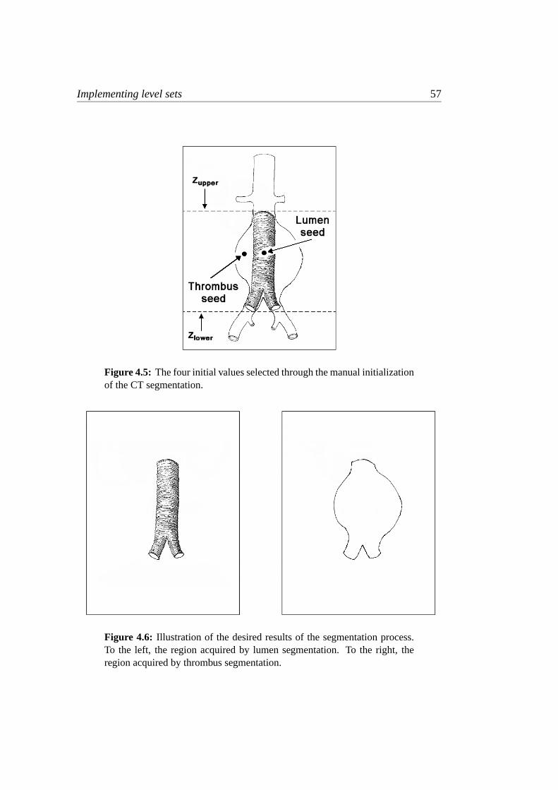
Implementing level sets 57
Figure 4.5: The four initial values selected through the manual initializationof the CT segmentation.
Figure 4.6: Illustration of the desired results of the segmentation process.To the left, the region acquired by lumen segmentation. To the right, theregion acquired by thrombus segmentation.

58 Experiments and results
The desired outcomes of these two steps are illustrated in figure 4.6. When thesegmentation of a structure is completed, the processed subvolume is re-insertedin the correct position into a volume of the same size as the original input.
4.4.3 Automatic lumen segmentation
The lumen is segmented in 3D using the level set method.
The aortic vessel structure is generally not visible in all slices of the CT volumes.Especially, it tends to be obscure in the lower slices of the image, below the bi-furcation point. If the image volume is not delimited by the two slices, as shownin figure 4.5, the evolving level set region may eventually tend to grow into ir-relevant parts of the image or the segmentation may become inaccurate in imageregions where traces of the vessel structure gradually disappear. This will be ofno concern if a subvolume is properly delimited prior to segmentation.
When the lumen segmentation commences, a tiny initial volume is initializedaround the seed point. The initial volume may be of any shape, as long as itis completely confined within the edges of the lumen. The level set algorithm willthen grow a region from this initial volume until it occupies the aortic lumen inits entirety. At first, the small volume will expand evenly outwards. As the ex-panding region is constrained by the edges delimiting the lumen in the potentialimage, it will progress to expand mostly upwards and downwards. Eventually, itis contained by the two slices delimiting the subvolume, and the volume will stopgrowing. As the measured growth of the region drops below a specified limit, thelumen segmentation is ended.
4.4.4 Automatic thrombus segmentation
The thrombus is segmented in both 3D and 2D slice-by-slice using the level setmethod.
The thrombus is a much harder region to segment than the lumen. The outeraortic wall and the aneurysm may at times be very hard to distinguish from thesurrounding soft tissues, and edge information may be scarce or even missingfrom the potential image. In such cases we hope that the possibilities of curvaturerestriction in the level set algorithm will prove to be useful.
To segment the thrombus, the intensity value sampled from the thrombus seedpoint is initially used to mask the previously segmented lumen structure, so that

Implementing level sets 59
the traces of the lumen edges will be eliminated when a new potential image isproduced.
When we segment the thrombus, the obtained segmentation of the lumen is usedas the initial level set. This is practical as it is located completely within the bor-ders of the outer aortic wall. Since the masking procedure has now removed theedges which constrained the growing region when we segmented the lumen, theinitial level set will now expand freely until it is constrained by the next boundary,which is that of the outer aortic wall. The two selected slices delimiting the sub-volume constrains the volume expansion, as it did before. As when segmentingthe lumen, when the measured growth of the region falls below a specified limit,the segmentation stops and the thrombus segmentation is complete.
4.4.5 3D segmentation of the lumen
4.4.5.1 Overview
The goal of the 3D lumen segmentation is to segment the inner aortic wall. Thesegmented region will include the aorta through the lower abdomen, from belowthe renal arteries, to slightly past the bifurcation point in the lower abdomen, in-cluding the top of the iliac arteries.
4.4.5.2 Preprocessing
Figure 4.7 shows two examples of slices from the initial volume. As can be seenin this figure, the graylevel can vary quite substantially from voxel to voxel. Thismeans that even in regions where the graylevel intensity is relatively monotonouson a big scale, the intensity values can be quite variable between single adjacentvoxels. This is an unfortunate characteristic when we want to detect edges in theimage later on, since edges are marked by intensity changes in the image.
To remedy this problem, we first employ a smoothing filter. The gaussian filterblurs an image by reducing detail and noise at the voxel level, while leaving struc-tures and regions on a bigger scale relatively intact. The degree of smoothing isdetermined by the variance of the gaussian; a bigger variance means a greater de-gree of smoothing. Thus, a gaussian outputs a weighted average of each voxel’sneighborhood, with the average weighted more towards the value of the centralvoxels. The result of gaussian filtering can be seen in figure 4.8.

60 Experiments and results
Figure 4.7: Two initial slices from the same unfiltered volume. In the leftslice, taken from below the bifurcation point, the lumen can be seen as twobright round regions next to each other in the middle of the picture. In theright slice, taken from above the bifurcation point, the lumen is seen as asingle bright region.
Figure 4.8: Gaussian filtered image, created with DiscreteGaussianImage-Filter (variance = 0.9).

Implementing level sets 61
Through experiments, the range of values for the variance found to work best isin the range 0.75 to 1.0. By selecting values below this range, the potential imagewill tend to contain too much noise, reducing the quality of the segmentation.Selecting values above this range, leaves us with an image with washed-out edges,again reducing the quality of the segmentation, as the segmentation will tend to“leak” into surrounding areas more easily.
Experiments indicated that although an even greater degree of smoothing wouldbe necessary to achieve a better segmentation, further use of the gaussian filterwould reduce the quality of the edges too much. On the other hand, the medianfilter was found to accomplish the task of more smoothing quite well, and is there-fore applied to the gaussian filtered image for further effect.
The median filter iterates over each voxel in the image. For each voxel a medianvalue is calculated from a cubical region with radiusr around the voxel, whereris defined by the user. For a three-dimensional image, this region is typically acube containing(2r + 1)3 voxels. The median filter is a robust average, since asingle unrepresentative voxel in the neighborhood does not significantly affect themedian value. Also, since the median value is actually one of the voxels in theneighborhood, the median filter doesn’t create any new unrealistic voxel valueswhen the filter is crossing an edge with large differences in graylevel values, forexample. This makes the median filter much better at preserving edges than thevery closely related mean filter and the gaussian filter.
Experiments showed that if the gaussian filter is applied after the median filter theresult is an image with weaker edge characteristics, and, later on, the final imageis much more likely to be oversegmented. The result of applying the median filterafter gaussian filtering can be seen in figure 4.9.
After these initial steps to smooth the image, it’s worth observing that, at thispoint, the areas in the image, which are similar in intensity on a regional level,contain voxels that are much closer in intensity values than they were to beginwith. This is of course what we set out to achieve.
Thus, it makes sense to shift our attention from considering the image at the voxel-level to looking at things at the region-level. That is, in order to create the bestpossible potential image, we want the region of interest (the lumen in this case) tobe as distinguishable as possible in intensity from the surrounding regions, therebyincreasing the edge gradients. One way to accomplish this is to increase the imagecontrast.
Contrast enhancement of the image was implemented follows: First, two thresholdintensities are selected. All voxels with intensities below the lower thresholdtloweris set to the minimum intensity,imin (0 in our case), and all voxels above the upperthresholdtupper is set to the maximum intensityimax (255 in our case). Voxel

62 Experiments and results
Figure 4.9: Median filtered image, created with MedianImageFilter(radius = 2).
intensities in the range betweentlower andtupper are redistributed according to thefollowing equation:
ivoxel =ivoxel − iloweriupper − ilower
imax.
As already noted,imax is the maximum possible intensity value, andivoxel is theintensity of the voxel to be recalculated. The upper and lower threshold intensities,iupper, andilower, are given relative toimax by
ilower = tlower · imaxiupper = tupper · imax,
wheretlower andtupper are values between 0 and 1.
Adjusting contrast generally helps to reduce the impact of the varying intensitylevels introduced by the data conversion process described earlier. As a lot ofvoxels in the lumen region will be thresholded by the upper intensity limit in theprocess, the region becomes more uniform. Edges will also show up more clearly,and it is easier to distinguish between regions of significantly different intensities.Without adjusting the contrast at all, the segmentation will generally be poor orsometimes unacceptable with frequent undersegmentation. Adjusting it too muchwill usually lead to oversegmentation and generally a structure containing a sig-nificantly less detail than can be seen in the original image.
Thus, it is important to take great care when we adjust the intensity level usingthresholds in this way. Generally, we have attempted to adjust the contrast asmuch as possible, but without losing important details in the image. Contrast
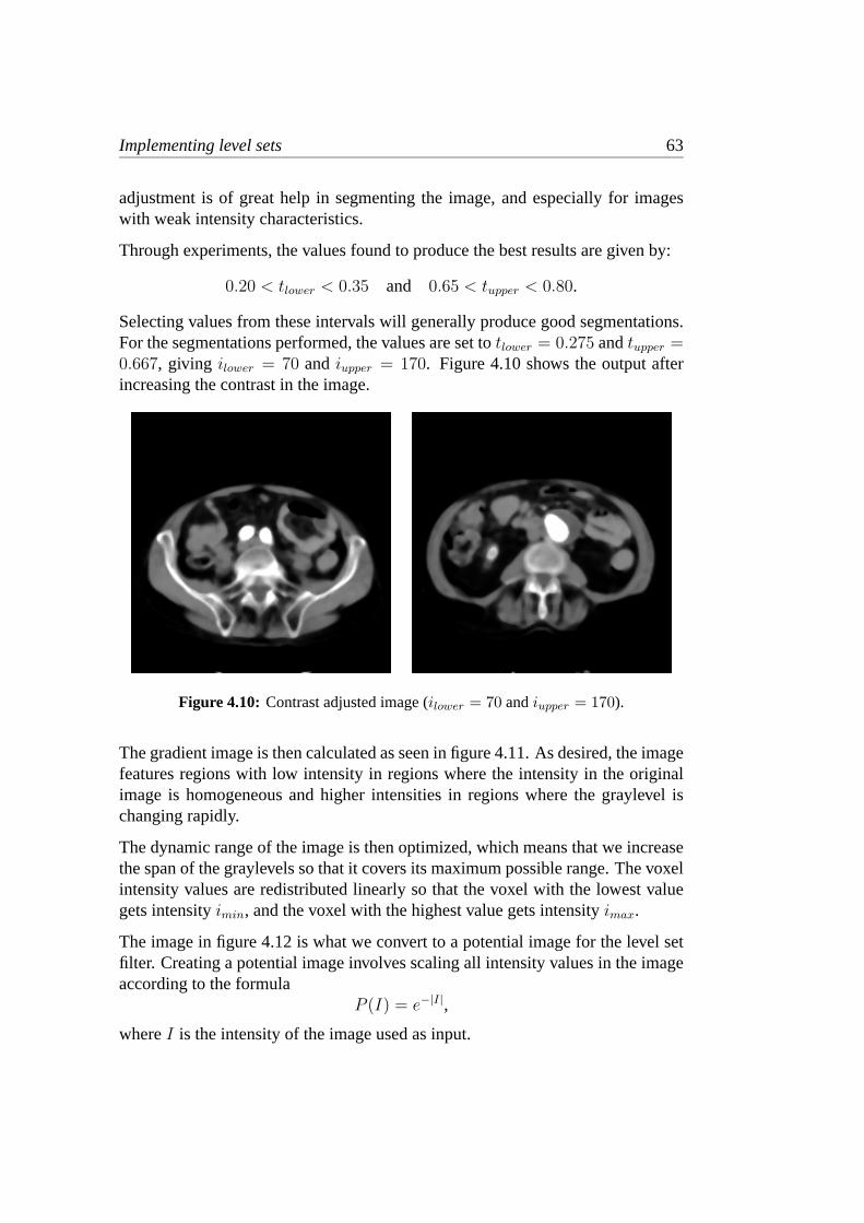
Implementing level sets 63
adjustment is of great help in segmenting the image, and especially for imageswith weak intensity characteristics.
Through experiments, the values found to produce the best results are given by:
0.20 < tlower < 0.35 and 0.65 < tupper < 0.80.
Selecting values from these intervals will generally produce good segmentations.For the segmentations performed, the values are set totlower = 0.275 andtupper =0.667, giving ilower = 70 andiupper = 170. Figure 4.10 shows the output afterincreasing the contrast in the image.
Figure 4.10: Contrast adjusted image (ilower = 70 andiupper = 170).
The gradient image is then calculated as seen in figure 4.11. As desired, the imagefeatures regions with low intensity in regions where the intensity in the originalimage is homogeneous and higher intensities in regions where the graylevel ischanging rapidly.
The dynamic range of the image is then optimized, which means that we increasethe span of the graylevels so that it covers its maximum possible range. The voxelintensity values are redistributed linearly so that the voxel with the lowest valuegets intensityimin, and the voxel with the highest value gets intensityimax.
The image in figure 4.12 is what we convert to a potential image for the level setfilter. Creating a potential image involves scaling all intensity values in the imageaccording to the formula
P (I) = e−|I|,
whereI is the intensity of the image used as input.

64 Experiments and results
Figure 4.11: Gradient magnitude image, created with GradientMagni-tudeImageFilter.
Figure 4.12: Gradient image with optimized dynamic range, created withRescaleIntensityImageFilter (OutputMinimum = 0, OutputMaximum =255).

Implementing level sets 65
Ideally, the resulting potential image has values equal to zero in regions with con-stant intensity and intensities close to one at the edges. In practice, this is hardto achieve perfectly, but as long as the edges delimiting the region of interest aremuch stronger than edge traces found in the interior of the region, this will gener-ally not be a problem.
4.4.5.3 Segmentation
After these preprocessing steps, we can finally initiate the segmentation. As a firstattempt at applying the level set approach, the fast marching method, describedin section 3.5.4.8 was tested (FastMarchingImageFilter in ITK). This special caseapplies to our problem because the speed of the evolving front we observe neverchanges sign, as it always moves outward from the initial level set. The advan-tage of this method is it’s speed, as it can do a segmentation much faster than thegeneral level set method. Its most serious drawback however, is that it does notencompass the same possibilities for restraining the curvature as does the generalmethod. Thus, it turns out to have a weakness very similar to that of the fuzzyconnectedness algorithm tested earlier, as the solution will tend to evolve intosurrounding regions even if only very small sections of edges are missing in thepotential image. This was quickly discovered upon testing the algorithm, as over-segmented images were frequently the result, and for this reason fast marchingwas abandoned in favor of the general level set approach.
The level set filter in ITK takes as input the potential image and the image of theinitial level set surface. A tiny volume in the shape of a3 × 3 cube is initializedaround the seed point. This initial volume of 27 voxels serves as the initial levelset. (A volume is initialized because the ShapeDetectionLevelSetFilter in ITK isunable to grow regions from a single voxel. This has no negative consequencesfor us, however.) A set of numerical parameters is also passed to the filter. Thesenumerical parameters will be further explained in the following.
The level set algorithm itself doesn’t specify any stopping criteria for the segmen-tation, as it is only a set of rules for how to evolve the relevant interface. Ratherthan just have the algorithm execute a large number of iterations, and then stop,stopping criteria are applied to halt the evolution of the solution to achieve thebest possible segmentation.
The implemented method works by having the level set filter iterate on the imagefor a specified number of iterations, after which stopping criteria are checked.If the stopping criteria are met, no further segmentation is performed, and thesegmented image is postprocessed. If not, the level set is reinitialized, using the

66 Experiments and results
currently segmented region as the new initial level set, and the iteration continuesagain for the specified number of iterations. This procedure goes on until thestopping criterion is met.
The implemented stopping criterion is based on a measure of the growth of thesegmented region, which is checked after the specified number of iterations. Thegrowth of the segmented region is measured as the ratio of the voxel count inthe most recently segmented region relative to that of the previous one. Thisratio is a numberr, where0 < r ≤ 1. The iteration stops whenr reaches acertain specified limit, which depends on the application and is found throughexperiments. Naturally, the typical ratio is a number close to 1, which indicatesthat the process will stop iterating when the solution evolves only very slowly orhas stopped evolving completely.
The exact parameters used for the 3D lumen segmentation are listed in table 4.1.These values were all determined by experimenting with the implemented setupuntil the values that produced the best results were found.
In the table, the parameters “iterations” and “ratio” are the same as those justdescribed. The parameters “epsilon” and “narrowband” were described in chapter3. The “timestep” parameter is related to the numerical implementation of thelevel set filter in ITK. Although details of the numerical implementation of theITK filters are not the focus of this text, a brief description of this parameter isprovided, since it is used explicitly: The timestep controls the speed at which thesolution is allowed to converge from one iteration to the next. The parameter isused to maintain stability in the solution by limiting the maximum change that avoxel can make in any one particular iteration. It must be low enough to keep thesolution stable, but should be high enough to keep the solution progressing at areasonable rate. (At some point in the future, functionality will be implementedin ITK to determine this parameter automatically.)
parameter iterations epsilon narrowband timestep ratiovalue 10 0.4 4 3 0.998
Table 4.1: The parameters used for the 3D lumen segmentation.
Selecting good values for the timestep, the width of the narrow band and the num-ber of iterations was done as follows: First, the value used for the timestep wasfound through experiments. For values higher than the one listed in table 4.1, thesolution would run the risk of becoming unstable, and for lower values, the so-lution would progress at a very slow rate. Generally, the progress of the solutionis slow, even for the highest timestep value that produces stable solutions. In thiscontext, “slow” means that the region will grow with too few pixels over one it-

Implementing level sets 67
eration so that the ratio measure will easily fluctuate too much to be useful as aconvergence criterion if it were to be checked after every single iteration. For thisreason, the highest possible timestep value was used.
Having found a good value for the timestep, the next issue was to determine anappropriate number of iterations to be executed between each time the stoppingcriterion is checked. The difference between the solutions of two consecutiveiterations, using the selected timestep, is still very small. To make it big enoughfor our stopping criterion to be viable, we increase the number of iteration betweeneach check. Starting with one iteration, the number of iterations was increaseduntil the solution evolved sufficiently between each condition check to make ourratio test for growth a reliable stopping criterion.
Having accomplished this, the last thing to do was to find the smallest possiblenarrow band that would contain the entire progress of the solution for the chosentimestep and iteration values. Starting with a narrow band of 10, this number wasdecreased as much as possible, while still containing the region evolved betweenthe chosen number of iterations.
Through experiments, it was determined that, for the same preprocessing steps,the final solution would be very similar by selecting different (reasonable andworking) sets of these three parameters. The primary gain lies in a much fasterconvergence to a final solution if a good set of parameters is selected. For anunfortunate selection of parameters, finding a solution may take hours, while fora good selection, a solution can be found in a matter of minutes (on a fast PC).Generally, for these three parameters, the same values were found to work equallywell when segmenting the thrombus in 3D and 2D later on.
Regarding the epsilon value, the edges of the lumen structure are generally veryclear and discernable, and the places where edge information is lacking are usu-ally few and far between. As explained in chapter 3, the epsilon value regulatesthe curvature of the expanding front. A greater value indicates that the front willtend to evolve more smoothly and uniformly. This has the advantage of keepingthe region from leaking through gaps in the potential image in places where edgefeatures are weak. Choosing a too big epsilon, close to 1, can make the segmen-tation stop before the narrowest parts of the aortic structure are fully segmented.This can typically happen in the iliac arteries in the bottom of the image. Select-ing very small values, closer to 0, might cause the solution to evolve into regionson the outside of the lumen, but because of the generally good quality of the po-tential images, this was found to occur rarely, even for small values of epsilon.In this case, finding a value for the parameter that produced a good solution wasrelatively easy.

68 Experiments and results
As for the value of the ratio parameter, experiments showed that it was unproblem-atic to select a value very close to 1, as the progress of the solution (and hence thegrowth of the segmented region) would drop off rapidly as the confining edges ofthe potential image were reached. Several values were tested for segmenting thetest data, and the value producing the most accurate segmentations was chosen.
The output of the level set filter is a binary image as seen in figure 4.14. A displayof the evolution of front of the region can be seen in figures 4.15 and 4.16.
initialize 3D level setwhile (stopping criterion not met){
reinitialize 3D level setfor (number of iterations){
do one level set iteration}
}
Figure 4.13: Pseudocode for the 3D level set segmentation of the lumen.
Figure 4.14: Slices from the 3D level set filtered image, created with Sha-peDetectionLevelSetFilter. (The numerical parameters used are listed in ta-ble 4.1.)

Implementing level sets 69
70 Experiments and results
Figure 4.15: 3D level set filtering of the lumen, showing the evolution of thesolution. From top left to bottom right, the images show the initial cubicallevel set and the segmented lumen region after 10, 20 and 30 iterations.

Implementing level sets 71
Figure 4.16: 3D level set filtering of the lumen, showing the evolution ofthe solution. From top left to bottom right, the images show the segmentedlumen region after 40, 50, 60 and 100 iterations. The lower right image isalso the final solution.

72 Experiments and results
4.4.5.4 Postprocessing
In the postprocessing step, we wish to improve the shape of the segmented region,remove sharp corners and generally smooth the edges of the segmented region sothat it conforms better to the actual anatomy of the lumen. A variety of techniquesfor smoothing the edges of the segmented region were tested, among them gaus-sian filtering with thresholding, dilation and erosion filtering and median filtering.(Using Fourier filters was also thought of, but ITK doesn’t yet contain any func-tionality for Fourier filtering.) Of these methods, the median filter was the filterproducing the best results. The problem with the median filter however, is that itis very slow, especially when the filter radius is big and the image to be filtered isin 3D. Specifically, even using a relatively small radius of 2 (or 3 later on) meansthat the filter, for each voxel in the image, has to sort a total of 125 and 343 vox-els respectively. The typical CT test image contains about108 voxels. Using theMedianImageFilter in ITK, with a radius of 3, this task took approximately 15minutes (on a fast PC).
Figure 4.17: Binary median filtered image, created with BinaryMedianIm-ageFilter (radius = 2).
Rather than dismiss the filter completely (which would also have implied lesssatisfactory results) because of its time penalty, it was decided to try to find away of increasing performance specifically for filtering of binary images. Theoptimized filter developed uses the following two facts:
• Only the subportion of the image containing the segmented object needs tobe filtered.
• Since the image is binary, the median can be obtained by simply counting

Implementing level sets 73
the voxels rather than sorting them. When more than half the voxels in aneighborhood has been found to be of either one of the two intensity valuesrepresented in the image, the median has been obtained.
Using these optimizations, the new BinaryMedianImageFilter processed theaforementioned image in about 30 seconds, producing the exact same results.The filter was subsequently submitted to the ITK developers and included in ITK[BINAR-02]. The binary median filtered image is shown in figure 4.17.
The end result of the lumen segmentation, a rendered 3D model of the obtainedregion, can be seen in figure 4.18.
Figure 4.18: Rendered model of the lumen region segmented using levelsets in 3D.

74 Experiments and results
4.4.6 3D segmentation of the thrombus
4.4.6.1 Overview
The 3D thrombus segmentation is performed by using the segmentation of thelumen as the initial level set, advancing the position of the front outwards in asimilar manner as before until it is constrained by the edges of the outer aorticwall and the stopping criterion is met.
4.4.6.2 Preprocessing
To begin with, the same preprocessing steps as were used for segmenting thelumen were tested. However, the resulting segmentation turned out to be unsatis-factory. This was mostly due to the contrast enhancement, which would tend toenhance differences between graylevels in the thrombus, thus amplifying inten-sity variations that lead to unfortunate characteristics in the potential image. Adifferent preprocessing pipeline had to be devised for the thrombus segmentation.
Figure 4.19 shows two slices from the initial image.
Figure 4.19: Slices from the initial unfiltered image.
When the thrombus is segmented, we want to make sure that there are no interfer-ing edges between the initial level set and the thrombus border. For this reason,we need to mask the brighter voxels of the lumen region to the darker intensitiescharacteristic of the thrombus region surrounding it. Thus, the edges of the lumen

Implementing level sets 75
won’t interfere when we segment the outer aortic wall, as they will be eliminatedfrom the potential image.
The masking is done as follows: First, the segmented lumen structure is veryslightly dilated by using a gaussian, so that it covers slightly more voxels thanwere actually segmented. This is done to ensure that all the brighter pixels thatproduce edge traces around the lumen region will be masked. The voxels of thisdilated structure are then copied into the CT image subvolume using the intensityvalue of the thrombus seed. The actual intensity value of the thrombus seed pointis determined by selecting the median intensity from a3 × 3 × 3 neighborhoodin the initial image 4.19, with this neighborhood centered on the seed voxel. Theresult after pasting the slightly expanded lumen region into the initial image canbe seen in figure 4.20.
Figure 4.20: Slices from the initial image after the segmented region hasbeen masked.
Care must be taken to not dilate the region too much, as we will run the risk ofmasking pixels outside the thrombus region. On the other hand it’s important notto mask too small an area, as segmentation of the thrombus will be much moredifficult if traces of the lumen edges remain inside the region of interest. Fromexperiments, the value found to dilate the area by an appropriate amount is avariance of 0.1. (An obvious alternative to this procedure would be to mask thelumen area in the lumen gradient image directly, thereby eliminating the need forthe intensity sample of the thrombus as well. In practice, this approach turned outto result in a very poor segmentation, as the edges of the thrombus are generallynot very clear in the edge map of the lumen.)
After masking, all voxels with intensities aboveiupper are thresholded by setting

76 Experiments and results
their intensity value toiupper, as seen in figure 4.21. Note that this is the same valueas used for the upper threshold for contrast enhancement in the lumen segmenta-tion. As this is an automatically computed threshold, it is not accurate enough tobe effective for removing the lumen edges without the prior masking. However,used in combination, these two steps were found to remove enough of the tracesof the lumen region for the thrombus segmentation to proceed without significantproblems.
Figure 4.21: Intensity values aboveiupper = 170 have been thresholded off.Voxels with intensities above this limit have all been set toiupper.
We apply the gaussian operator on this image to reduce intensity variations on avoxel-to-voxel scale to obtain more uniform regions. The result of this step canbe seen in figure 4.22.
In figure 4.23 we have used the median filter for further smoothing. Again, apply-ing a median filter for smoothing proved to make regions with similar intensitiesmore uniform and edges are better preserved compared to simply increasing thevariance of the gaussian operator.
The gradient magnitude image calculated is shown in figure 4.24.
We then optimize the dynamic range of the edge image in exactly the same wayas we did when we segmented the lumen. The result can be seen in figure 4.25.

Implementing level sets 77
Figure 4.22: Gaussian filtered image, created with DiscreteGaussianImage-Filter (variance = 1.0).
Figure 4.23: Median filtered image, created with MedianImageFilter(radius = 2).

78 Experiments and results
Figure 4.24: Gradient magnitude image, created with GradientMagni-tudeImageFilter.
Figure 4.25: Gradient image with optimized dynamic range, created withRescaleIntensityImageFilter (OutputMinimum = 0, OutputMaximum =255). Note how different the edge features in these slices are from thoseshown in figure 4.12, especially how the traces of the lumen have been re-moved and those of the thrombus are more prominent.

Implementing level sets 79
4.4.6.3 Segmentation
The preprocessed image is then passed on to the level set filter to be used as thepotential image. The model of the lumen segmented in section 4.4.5 is also inputto the filter, as the initial level set. The parameters used for this segmentation arelisted in table 4.2.
parameter iterations epsilon narrowband timestep ratiovalue 10 0.6 4 3 0.994
Table 4.2: The parameters used for the 3D thrombus segmentation.
Note that a slightly bigger epsilon-value is used this time, compared to the 3Dlumen segmentation. The reason for this is that the edges of the thrombus aremuch less prominent in the potential image than was the case with the lumen.Much bigger portions of the edges will be missing, and there is a greater need torestrain the expansion of the solution. Decreasing the parameter below the valuein the table easily causes the segmented region to expand beyond the borders ofthe thrombus. Increasing it, however, sometimes lead to undersegmentation as theregion stops expanding before the edges of the thrombus are reached.
The ratio parameter used for the stopping criterion is slightly smaller than theone used for the lumen segmentation. The reason for this is that the edges of thethrombus are of lower quality than those for the lumen, and it was observed thatthe solution can grow very slowly for a very long time before it stops and evenexpand beyond the edges if the ratio is set too high. The listed value was obtainedthrough experiments and is set so that we get the most accurate segmentation. Ifset lower, the segmentation may terminate prematurely with undersegmentationas the result, and if set higher, oversegmentation is more likely to happen.
As mentioned previously, the other parameters values were found to work well,so no additional changes were needed. The resulting output of this step is shownin figure 4.27.

80 Experiments and results
initialize 3D level setwhile (stopping criterion not met){
reinitialize 3D level setfor (number of iterations){
do one level set iteration}
}
Figure 4.26: Pseudocode for the 3D level set segmentation of the thrombus.
Figure 4.27: Slices from the 3D level set filtered image, created with Sha-peDetectionImageFilter. (The numerical parameters used are listed in table4.2.)

Implementing level sets 81

82 Experiments and results
Figure 4.28: 3D level set filtering of the thrombus, showing the evolution ofthe solution. From top left to bottom right, the images show the initial levelset and the segmented region after 10, 20 and 30 iterations. Notice that theinitial level set is the same as the segmentation shown in figure 4.18

Implementing level sets 83
Figure 4.29: 3D level set filtering of the thrombus, showing the evolution ofthe solution. From top left to bottom right, the images show the segmentedregion after 40, 50, 70 and 90 iterations. The lower right image shows thefinal segmentation.

84 Experiments and results
4.4.6.4 Postprocessing
Again, we smooth the edges using a binary median filter. The obtained region ismore rugged this time, caused by the fact that the small variations in the potentialimage, inside the region of interest, are relatively big compared to the potential ofthe edges. (Remember that these variations was not a problem when segmentingthe lumen because the characteristics of the lumen edges were so strong.) Thus,the need for postprocessing the result is more urgent, so a bigger radius is usedin the binary median filter. The processed output can be seen in figure 4.30. Therendered end result of the thrombus segmentation is shown in figure 4.31.
Figure 4.30: Binary median filtered image, created using the BinaryMedi-anImageFilter (radius = 3).

Implementing level sets 85
Figure 4.31: Rendered model of the thrombus region segmented using levelsets in 3D.
4.4.7 2D segmentation of the thrombus
4.4.7.1 Overview
The 2D thrombus segmentation is also performed by using the segmentation ofthe lumen as the initial level set. This time, however, we segment the thrombusslice-by-slice, using the slices of the segmented lumen as the initial level sets.After all the slices are segmented, they are inserted into a volume of the same sizeas the original input to produce a 3D model.

86 Experiments and results
4.4.7.2 Preprocessing
The preprocessing stage for this segmentation is exactly the same as for the 3Dsegmentation of the thrombus described in section 4.4.6.3.
4.4.7.3 Segmentation
The parameters used for this segmentation are listed in table 4.3.
parameter iterations epsilon narrowband timestep ratiovalue 10 0.8 4 3 0.995
Table 4.3: The parameters used for the 2D thrombus segmentation.
Compared to the 3D segmentation of the thrombus, the epsilon value has beenincreased. When segmenting in 2D, a bigger value for epsilon is needed to achievesimilar results compared to when 3D segmentation is performed. In 3D, when thealgorithm is confronted with a section of the thrombus where edge characteristicsare weak, the algorithm will apply the curvature restraint globally. Frequently,edge traces are weak only in a few consecutive slices at a time, which often makesfor areas with low potential that are small in height, but bigger in width. In thesecases, it is clearly easier to contain the evolving front if the curvature restraint isapplied to the whole region rather than independently to successive slices. Thus,a larger epsilon turned out to be required when segmenting in 2D.
Only a minor adjustment is performed on the ratio parameter, compared to the 3Dthrombus segmentation. This is done mostly to compensate for the fact that theuse of a bigger epsilon generally requires more iterations to evolve into a similarsolution, mostly because the evolving front doesn’t pass obstacles in the potentialimage as easily, and therefore expands at a slower rate.
Again, the other values were found to work well, so no changes were needed.

Implementing level sets 87
for (all slices){
initialize 2D level setwhile (stopping criterion not met){
reinitialize 2D level setfor (number of iterations){
do one level set iteration}
}}
Figure 4.32: Pseudocode for the 2D level set segmentation of the thrombus.
Figure 4.33: Slices from the 2D level set filtered image, created using theShapeDetectionImageFilter. (The numerical parameters used are listed intable 4.3.)

88 Experiments and results
Figure 4.34: 2D level set filtering, showing the evolution of the solution inone of the slices. From top left to bottom right, the images show the initiallevel set and the segmented region after 10, 30 and 60 iterations. The lowerright image shows the final segmentation.

Implementing level sets 89
Figure 4.35: 2D level set filtering, showing the evolution of the solution inanother of the slices. From top left to bottom right, the images show thesegmented region after 10, 30 and 130 iterations. The lower right imageshows the final segmentation.

90 Experiments and results
4.4.7.4 Postprocessing
In this case, also, the segmented image is postprocessed in the same way as de-scribed in section 4.4.6.4. The binary median filter was found to be very good forprocessing the 2D segmented thrombus image, since using the median voxel ofa neighborhood easily eliminates extreme protrusions or dents in the segmentedregion caused by single unrepresentative slices. The result of the median filteringis shown in figure 4.36. A rendered model of the outer aortic wall is displayed infigure 4.37.
Figure 4.36: Binary median filtered image, created with BinaryMedianIm-ageFilter (radius = 3).

Implementing level sets 91
Figure 4.37: Rendered model of the thrombus region segmented using levelsets in 2D.
4.4.7.5 The segmentation error
To evaluate the results of the volumetric segmentations performed, it is desir-able to measure the difference of the segmented regions to the actual anatomicalregions. The segmented region is usually compared slice by slice to the actualregion segmented manually. As no manual segmentation of the test images ex-isted, they would first have to be segmented manually if an error estimate was tobe produced. However, since manually segmenting both the inner and outer aorticwalls from all three test images (all of which contain well over 100 slices) wouldhave been an excruciating and extremely time-consuming task, a compromise wasmade to select five slices from each test image. In these five slices, both the inner

92 Experiments and results
and outer aortic walls were extracted manually, and these manual segmentationswere then compared with the equivalent slices from the automatically segmenteddata.
In all three cases the five slices were selected as follows: Slice 1 is the fifth fromthe top of the volume, while slice 5 is the fifth from the bottom of the volume.Slice 3 is located at the point where the diameter of the aneurysm is at a maximum,and slices 2 and 4 are located 15 slices above and below slice 3, respectively.Figure 4.38 shows an illustration of the location of the five slices.
Figure 4.38: Illustration of the positions of the five slices used to calculatethe segmentation error.
To measure the error in a slice, a center pixel is selected at the same index inboth the manually and automatically segmented slices. Horizontal and verticallines are then traced in both slices until they reach the edges of the manuallyand automatically segmented regions. The distance from the center, measured inpixels, is then recorded. The error, denoted byd, is the positive difference betweenthe distances in the automatically segmented slice and the equivalent distances inthe manually segmented slice. In the slices where we have a bifurcated structure,this process is done twice, once for each of the aortic branches. An illustrationcan bee seen in figures 4.39 and 4.40.
When the errorsd1 to d4 (andd5 to d8 for slice 5) have been found, the mean errorfor each slice is calculated as:
1
n
n∑i=1
dn,
wheren is the number of distances measured in the slice (4 or 8).

Implementing level sets 93
Figure 4.39: Illustration of the error measures in slices 1-4, above the bifur-cation point.
Figure 4.40: Illustration of the error measures in slice 5, below the bifur-cation point. In this case, the segmentation error is measured separately forboth of the iliac arteries.

94 Experiments and results
The error in millimeters is found by multiplying each result by the pixel spac-ing. The pixel spacing is the spatial extent of one pixel, in our case measured inmillimeters, given as one number for each spatial dimension.
The measured segmentation errors in millimeters are listed in table 4.4. Moredetailed data for the slices of each image can be found in appendix A.
segmentation 1 2 3 4 5 alllumen 3D 0.47 0.22 0.71 0.70 1.05 0.63thrombus 3D 1.95 1.05 1.41 1.61 2.02 1.61thrombus 2D 2.17 1.17 1.41 1.36 1.82 1.59
Table 4.4: Error measures in millimeters of the different segmentations.The values in each row are averaged over the three segmented test images.
4.5 Implementing mutual information optimization
4.5.1 Background
We want to perform 3D rigid registration using the mutual information metric.Rigid registration means that only translation and rotation of the two images areperformed to align them. No scaling is performed, as the scale of the CT and USimages are already equivalent. This implies that if the distance between the sametwo anatomical points in the two images are measured in voxels and multipliedby their respective voxel spacings, the distance measured in millimeters will bethe same. Unfortunately, no satisfactory results were obtained using the currentframework for mutual information registration in ITK.
4.5.2 The CT and US image modalities
As noted earlier, the CT data is acquired from patients with injected contrast en-hancement. In these images, the graft and the lumen appears as a solid region ofbright voxels. The aneurysm around it appears as a region of darker voxels. Thecontrast between the lumen and the thrombus is generally good, while the contrastbetween the thrombus and surrounding tissues can be much more diffuse.

Implementing mutual information optimization 95
Figure 4.41: CT and US images of similar features in the abdomen prior tomanual extraction of the subregions to be registered. The CT and US imagesare from corresponding data sets. While the lumen and the thrombus showup as solid regions in the CT images, it is the edges of these structures thatare the most predominant features in the US images. The lower right USimage also illustrates how US data is often very degraded by noise.

96 Experiments and results
In the US images, the AAA and the stent graft are the most predominantly visiblestructures, and there is hope that these structures can be used as the main featureto register the images. The metal structure in the graft gives a high amplitudeecho in the US images, and so does the outer aortic wall. These regions show upas bright voxels, while the space between the graft and the outer aortic wall hasdarker intensity.
These different characteristics are illustrated in the images in figure 4.41. In gen-eral, the intensity maps for CT and US images are very different in that structuresthat are bright in the CT volume may be less bright or even close to black inthe US volume. The application of many other common registration techniqueswould easily lead to confusion as structure intensities and other image character-istics don’t match directly. Thus they would have great difficulties matching theright structures to each other. The appearance of bright edges in the US imagecould easily be confused with structures that are bright in the CT volume, such asbone tissue, for example.
4.5.3 Registering CT and US images
4.5.3.1 Manual preparations
The available ultrasound test data were already resampled to the equivalent of theCT image resolution. Since the CT image is so big compared to the original USimage (see section 4.1), the resampled ultrasound image will contain a majorityof black voxels, with a relatively small region of actual ultrasound data inside it.
CT images generally also contain a lot of black voxels, as demonstrated in picturesthroughout this text.
If these images are registered the way they are, the large regions of black voxelswill influence the mutual information metric in an undesirable way, as they gen-erally do not contain information about the anatomical region of interest. Whenvoxels are sampled, as explained in section 3.6.2.3, there will be a significantnumber of (black, black) and (black, non-black) pairs which do not contain pa-tient information. (Of course, the effect is negative not because the voxels areblack, but because black voxels will mostly be sampled from regions in the im-ages that doesn’t contain information relevant for registering the images. Blackvoxels located within the image regions that actually represent anatomical dataare not a problem.)
To exclude the problematic regions of black voxels from the computation, a small

Implementing mutual information optimization 97
subvolume is extracted from both the CT and US images. These two subvolumesare of the same size and contain the CT and US voxels from corresponding voxelindices respectively. The volumes are delimited so that they contain only voxelsthat represent actual anatomical data obtained from the patient.
4.5.3.2 Full automatization
Since the issue of automatization is important in this report, an explanation isprovided on how this procedure is intended to be fully automated, without theneed for manual extraction of subvolumes from the CT and US images.
Although the US images available for use in this project were resampled to thesame resolution as the CT images, the US images will generally not be resampledthis way, and they will contain only voxels from within the patient’s abdomen.When the initial transform is executed to initially align the two images beforethe registration procedure starts, the ultrasound image, which in the un-resampledform is much smaller than the CT image, will be transformed into a region of theCT that contains a majority of relevant voxels. Thus, the irrelevant black pixelsinitially causing problems here will generally not be an issue. (Naturally, thesample pairs used by the mutual information metric will always have to residewithin the region of the smallest of the two images to be registered. The initialregistration performed by the positioning system is accurate enough so that, afterthe initial transformation, the volume alignment will generally be good enough tomake the risk of sampling too many irrelevant voxels a non-issue.)
When registering images in ITK, it is usually favorable to take advantage of thefact that the role of the moving image and the fixed image is not symmetric. Thismeans that when the CT is the fixed image and the US is the moving image, theregistration process will behave differently compared to when the roles of the twoimages are interchanged.
As described in section 1.7.1, the registration process basically takes voxels fromthe fixed image and map their spatial location through the registration transforminto the geometric space of the moving image. It is best to use the US as the fixedimage since such a setup is more favorable. The reasons for this has to do with theresolution of the image data. The US images typically contain around107 voxels,while the converted CT data contain about108 voxels. As mentioned earlier, bothare 8 bit grayscale.
If the CT is used as the fixed image, each evaluation of the metric will need to visit108 voxels. (When using the full-size DICOM CT data, this number will easilygrow by an order of magnitude.) Most of the voxels will end up being mapped

98 Experiments and results
to the outside of the ultrasound image, thus not at all contributing to the metric,while still using a lot of processing time.
If, on the other hand, the US is used as the fixed image, the computation of themetric will be visiting about107 voxels. Most of them will be mapped to regionsof the CT image that contain relevant information, thus they are very likely tocontribute to the metric.
(Specifically, when using the mutual information metric this not exactly true, sincea precise number of voxels are selected and the metric is computed only for thosepixels. For the use of most other metrics however, this is a fact important to beaware of.)
Another advantage of exchanging the role of the images is that the derivative ofthe metric uses the gradient of the moving image, and it is generally better to usethe gradient of the CT image than the gradient of the US image. This is alsoanother reason for using the CT image as the moving image.
Other than this, interchanging the role of the fixed and moving images will simplyresult either in a final transformT or its inverseT−1.
4.5.4 The registration procedure
The registration framework in ITK is modular, as explained in section 3.4.3. Thus,when composing a registration method, each component is relatively independentof the others. The most critical components though, are the metric and the opti-mizer.
Before the registration process is started, the images are normalized to have amean value of 0 and a standard deviation of 1. This is done to get the intensityvalues in the image on the standard form the mutual information metric workswith, and is remniscent of the way we converted gradient images into the potentialimages required by the level set filter.
The registration process is started by first applying the initial offset transforma-tion, which has been produced by the marker and positioning system and is de-scribed in section 4.1.3. This aligns the images as accurately as the system wasable to record when the images were acquired. Of course, this initial transform isonly applied once, after which the registration method takes over to further refinethe image alignment.
All the voxels in the fixed image are then mapped to the moving image using theselected registration transform.

Implementing mutual information optimization 99
As the voxel values are mapped into the moving image, their spatial position willgenerally be mapped to non-grid positions. This means that a mapped voxel doesnot overlap exactly with one of the voxels in the other image. The interpolatorthen helps determine what the voxel intensity should be.
After this, the metric, that is the mutual information in our case, then evaluateshow well features in the two images match each other. This is done by comparingthe moving image with the transformed fixed image.
Lastly, the role of the optimizer is to keep changing the parameters of the reg-istration transform, searching for a combination that gives the best value of themetric. Thus, the execution of the registration method is ultimately driven by theoptimizer.
perform initial transformfor (number of iterations){
transform fixed image to moving imageinterpolate voxelsevaluate mutual information metricevaluate optimizer
}
Figure 4.42: Pseudocode for the registration procedure.
A technique known as multiresolution registration was also employed. To saveprocessing time, both images to be registered may be downsampled to a lower res-olution, before the registration starts. Registration is performed on the downsam-pled images for a number of iterations before it continues on the full-resolutionimages. The technique is generalized so that the original images may be sub-sampled any number of times, to different resolutions. When the registration iscompleted on one level, it steps up to the next level and the images are registeredagain, and so on, until the full-resolution images are registered. This increases theperformance considerably compared to working with the full-resolution imagesall the time.
When multiresolution registration is used, the for-loop in figure 4.42 is executedonce for each level, as every single level in the multiresolution framework is acomplete registration in its own right.
The ultimate goal of the registration process is to find the set of values for thetransformation that optimize the metric. The output of the registration is a trans-formation matrix which can be used to resample the moving image to align it withthe fixed image.

100 Experiments and results
Following the advice of the ITK developers, two different optimizers were tested:the GradientDescent optimizer and the RegularStepGradientDescent optimizer.
4.5.5 Using the GradientDescent optimizer
The GradientDescent optimizer implements one of the many variants of gradientdescent. The central parameter in this optimizer is the learning rate. The learningrate is one of the hardest parameters to adapt in the entire process. It is used bythe Gradient descent in order to compute how long each step should be in theparameter space of the optimizer.
When we perform rigid registration in 3D, the parameter space is six-dimensional,consisting of a translation(x, y, z) and a rotation(γ, θ, φ).
The optimizer starts with a particular combination of(x, y, z, γ, θ, φ). It evaluatesthe metric for these values and the derivative of the metric with respect tox, y, zandγ, θ, φ. Using this derivative, the optimizer obtains a gradient direction inthis 6D parameter space(x, y, z, γ, θ, φ). The metric may then be improved bymoving in the direction of this gradient.
To find out how far to move, the GradientDescent optimizer computes the lengthof this movement by multiplying the metric-derivative vector by the learning rate.Naturally, the larger the learning rate, the longer the step will be.
Initially, the easiest thing to do is to use relatively small values for the learningrate. The size will depend on the values of the metric derivative because whatmatters in the end is the product of the metric derivative and the learning rate. Tofind good values for the learning rate, the following procedure can be used:
• First, an arbitrary value is selected, for example in the order of10−3.
• A registration is performed and the values of the transform from one iterationto the next is tracked.
• If the distance moved from one iteration to the next is too big, the learningrate is reduced.
• If, on the other hand, the distance moved is too low, the learning rate is in-creased.
A movement in the range of 0.1 to 10 voxels per iteration is usually preferred, butthis is dependent on the application and on the current degree of image alignment.
The value of the learning rate depends on the value of the metric derivative be-tween the two images. The metric derivative can only be found through testing and

Implementing mutual information optimization 101
depends on the nature and content of the images, as well as the type of transformused. Thus, the only way to find a good value is through experiments.
The learning rate of the GradientDescent optimizer has the serious drawback thatthe length of the step is proportional to the derivative of the metric, and it is prettyhard to get an idea of how this derivative will change as the registration evolves.For this reason, even if a good learning rate for the initial steps of the registrationis selected, the value may become inappropriate at any moment. In the same way,low gradient regions in the metric can easily make the step size too big. Theadvantage of this optimizer is that it is fast, and it is useful to experiment to findgood initial values for some of the registration parameters before switching to adifferent and more robust optimizer.
4.5.6 Using the RegularStepGradientDescent optimizer
The RegularStepGradientDescent optimizer also uses the metric derivative to de-termine in which direction to move. However, this optimizer applies a differentstrategy for computing the step size. The regularStepGradientDescent uses anindependent, user provided, initial value for the step.
This optimizer computes the derivative of the metric with respect to(x, y, z, γ, θ, φ)and normalizes it, so that only the direction of the derivative is used, and not itsmagnitude. This normal vector is then multiplied by the initial step value providedby the user. This way the first step will always be what the user specified amountof voxels, completely independent of the value of the metric derivative.
The optimizer will continue using this step size until it advances one step withoutany improvement of the metric value. At this point, the optimizer steps back, andthe current step size is multiplied by -0.5, so that its direction is reversed and thestep size is halved. It then proceeds as before, again advancing until the metricstops improving.
Every time that the direction changes more than 90 degrees, the step length isdivided by two. A good initial value for rigid transforms is 0.1, which is equivalentto a moderate rotation of about 5 degrees.
The algorithm stops when the step size reaches a minimum value, also providedby the user.
This is generally a more robust method than the GradientDescent optimizer, withthe drawback that it is much slower.

102 Experiments and results
4.5.7 Parameter selection
After selecting a metric and an optimizer, the parameters for the chosen methodsthat produce the best results must be determined. In general, the most difficulttask in registration is to find a good combination of parameters for the problem.The challenge lies in finding the parameters that fine-tune a particular approachfor a particular application.
Through correspondence with the ITK developers, it was learned that the selec-tion of these parameters is a huge and very lengthy process of trial and error. Asof today, there are no documented rules or directions for tuning the parameters forthe use of mutual information. According to ITK developers, it appears that inthe past, the importance of documenting the process of parameter tuning for thistechnique has passed relatively unnoticed. As a consequence, the default parame-ters for mutual information provided in ITK are mostly those found through initialtesting and experiments performed during development.
Mutual information is estimated using two sample sets: one to calculate the singu-lar and joint probability density functions and one to calculate the entropy integral.By default 50 samples points are used in each set in ITK. In our tests, values be-tween 50 and 80 were used, according to the recommendations of the developers.Using more sample points would make the process extremely slow, running forhours.
A gaussian kernel was used in the density estimation in the mutual information.The quality of the density estimate depends on the choice of the kernel’s vari-ance. The optimal choice will depend on the images in question. It can be shownthat around the optimal variance, the mutual information estimate is relatively in-sensitive to small changes of the variance. Experiments performed by the ITKdevelopers have shown that a variance of around 0.4 works well for images nor-malized to have a mean of zero and a standard deviation of 1.0. Variances in therange 0.3 to 0.5 were tested.
Selecting the right parameters for the optimizer is critical to reach a good result.According to the ITK developers, the only way to find what values give the bestresults is to experiment, using different values for the learning rate in the case ofthe GradientDescent, and the initial step value in the case of RegularStepGradi-entDescent. The step size and learning rate values used in our tests were both inthe order of10−6 to 101.
The number of iterations in the registration can be set to any amount. A numberof iterations in the orders of103 to 104 were tested, and using a number smallerthan in the order of103 was not recommended, as the images would not have timeto align.

Implementing mutual information optimization 103
The number of levels for multiresolution registration can also be varied. Thenumber of levels used in our tests were between 1 and 4.
A parameter value is also used to scale between the translation and rotation pa-rameters. This parameter is dependent on the images, and has to do with howmuch the edges of an image will move as a result of the image being rotated aboutits center. It was recommended that this value be set to approximately the voxelspacing in millimeters, and values of this order of the voxel spacings were tested.
4.5.8 The problems
Despite collaboration with the supervisors at Sintef Unimed and extensive cor-respondence with the developers of ITK to find a good set of parameters, it hasso far been found extremely difficult to register US to CT using the registrationmethods currently available in ITK.
Using the GradientDescent optimizer with small learning rates of10−6 to 10−5,the registration will move arbitrarily. It never reaches the correct position, andthe steps are very small, in the range10−2 to 10−1. The result is fluctuationsaround the starting point in a random way. Using multiresolution registration,or changing the other parameters did not produce any observable improvementsin the outcome. When the learning rate is increased up to a certain threshold(about5 · 10−4 to 1 · 10−3), the step size becomes too big, and the algorithmwill consistently move the two images apart until their respective spatial regionsare completely disjoint. The values of the transform were checked after eachiteration, but there was generally a consistent lack of any pattern to the movementand direction of the image.
Tests performed with the RegularStepGradientDescent optimizer showed that, re-gardless of the initial learning rate used, the algorithm would consistently movethe two images apart until their respective spatial regions were completely dis-joint. Again, applying the multiresolution technique and considerably changingthe set of parameters did not produce better results or observable improvements.
4.5.9 Attempted corrections
Initially, the CT and US images to be registered were not preprocessed in any waybefore the registration process started. Using a gaussian to blur the CT and the USimages was tested, using variances between 0.6 and 1.0.

104 Experiments and results
Smoothing either or both images before registering was also tried, but did notlead to observable improvements in the results. Attempts at registering the gra-dient map of gaussian smoothed CT rather than the original CT were also made.Unfortunately, none of these changes led to any observable improvement in re-sults.

5 Discussion and conclusions
In this chapter, we discuss our findings and results on the use of ITK for medicalsegmentation and registration and sum up our work. A conclusive evaluation ofITK is also provided.
5.1 Segmentation
The segmentation scheme presented in this report performs automatic segmenta-tion of both the inner and outer aortic wall in postoperative CT images of patientswith AAA, using 2D and 3D level sets, requiring the manual initialization of onlyfour values. The spatial extent of the segmentation includes a region from belowthe renal arteries to the top of the iliac arteries, including the aortic bifurcationpoint in the lower abdomen.
The inner aortic wall has been segmented using the level set method in 3D. Theaverage segmentation error in this case is 0.63mm, which implies that sub-voxelaccuracy has been achieved. The outer aortic wall has been segmented using thelevel set method in both 3D and 2D. In this case, the average errors measured were1.61mm and 1.59mm respectively. This is an error margin of slightly more thanone voxel. The segmentation error for the inner aortic wall is generally smallerthan that of the outer aortic wall, and this can mainly be attributed to the muchlower visibility of the outer aortic wall in the CT images.
Although schemes to segment AAA using level sets are also presented in[LONCA-01] and [MAGEE-00], these do not focus on, or detail, how to auto-mate the presented methods. The deformable model scheme for semi-automaticsegmentation presented in [BRUIN-02], produces a segmentation with a smallererror, compared to the one presented in this text, but also requires extensive man-ual initialization and user intervention. It also avoids the challenges associatedwith the aortic bifurcation by segmenting the dilated aortic tissue only. Further
106 Discussion and conclusions
searches indicate that an automatic scheme for segmentation AAA such as theone documented in this report, has not previously been presented.
More testing needs to be performed to determine whether it is best to use levelsets in 2D or 3D for segmentation of the outer aortic wall. The current resultssuggest that the error is very similar for both. However, it is easier to imposevarying structure constraints when segmenting slice-by-slice, as conditions maybe imposed on each individual slice when segmenting in 2D. This is in contrast tothe 3D segmentation where the whole volume is handled as one single structure.
Using the current framework for level set segmentation in ITK and the availabletest data, it is likely that the achieved results are close to as good as one canrealistically expect. As ITK is further developed, there are good prospects forimprovement of the scheme in the future.
5.2 Registration
A scheme to perform automatic registration of CT and US images of AAA usingmutual information has been discussed. The tests performed indicate that an ap-proach using the framework currently available in ITK, may not by be sufficient.Despite intense collaboration at Sintef Unimed and extensive correspondence withthe developers of ITK, no set of parameters providing satisfactory registration ofthe CT and US data was achieved.
While the process of determining the right parameters for the registration is indeeda huge process of trial and error, the fact that no improvement in results wasobserved, despite using parameter values as recommended by the ITK developers,is alarming. Between the extreme cases of the registration fluctuating randomlyabout its initial state and the two volumes moving completely apart, it would bereasonable to expect to see the registration moving in a way more or less consistentwith our intentions. This was not found to be the case and was never observed.These results may be due to several factors.
The quality of the ultrasound data may be too poor, with too much noise, so thatthere is simply not enough mutual information in the sample pairs from the CTand US images for the mutual information algorithm to actually register them.Similarly, the converted CT data has been downsampled and contain only 25 % ofthe original information. Performing registration using the original CT data ratherthan the converted data would also be interesting. Using the original image dataof higher resolution and without intensity artifacts may possibly produce betterresults. Although mutual information is basically immune to the differences in

Conclusive evaluation of ITK 107
graylevels due to the different image modalities involved, it cannot do much if theimages in question don’t actually have enough potential matching regions.
Exploring other algorithms, such as the one described in [ROCHE-01], may be aworthwhile option over the risk of spending months attempting to find workingparameters for a registration algorithm that may or may not be appropriate for theproblem. At this time though, this method is not available in ITK.
The mutual information method for registration is the most promising method theITK toolkit has for registration of CT and US images at the time of this work. Still,it may be that a different algorithm is needed to achieve better results. Althoughit may be desirable to perform further testing to confirm or deny the results of thework presented on registration of CT and US images in this text, it is likely thatthe methods of the existing registration framework available in ITK is insufficientfor registering the image data used in this project.
5.3 Conclusive evaluation of ITK
As mentioned in section 3.4.6, the development of this project is for the most partbased on intermittent versions of ITK released after the first beta. The first betabecame available in February 2002, shortly after this project was begun, and thesecond beta was ready in June. Although it was initially seen as desirable to staywith the beta version of ITK to ensure full compatibility between all the piecesof software written for this project, the increasing requirements for more complexfunctionality as development went on, intermediate development versions of thetoolkit had to be used instead. In practice, frequent upgrades were necessary toget access to new and essential functionality.
Although the first beta versions of ITK have been released, the software remainsin very active development, and the first fully developed version is still monthsaway. The sheer increase in the amount of source code well illustrates the pace ofdevelopment of the toolkit. Over the span of four months, from March to June, thecode base of ITK grew from 21MB to 32MB, an increase of more than 50 %. Itis not always easy to keep up with the latest development of such a large softwarepackage, and the constant process of development, redevelopment and modifica-tion of existing functionality may sometimes lead to undesirable situations for theend user.
Since of the code in ITK is still relatively new, the coding style isn’t always con-sistent, which means that it may be necessary to perform the same type of functioncalls in slightly different ways, depending on what filter or functionality is used.
108 Discussion and conclusions
This can make the API confusing, especially when the API is the only documenta-tion available much of the time. Also, new functionality is added and changed ona regular basis, which can make software development difficult. The typical sce-nario encountered is the one where new features are added to the software, whichthe at some point is found to be necessary to solve the problem the user is workingon. When an upgrade to the more recent version of the software is made, the newversion turns out to contain other changes as well, requiring further modificationof the user’s own code.
The whole level set code framework in ITK has also been under redevelopmentfor the full length of this work, and the current level set implementation, used inthis project, will eventually be removed from the codebase at some point in thefuture.
The lack of tutorials, books and documentation in general makes ITK difficult tolearn and use. Thus, there was quite some time of learning before useful code wasproduced for this project. Also, the lack of a DICOM reader and a general lack ofrobust IO-modules at the time the development of this project started, meant thatessential functionality to get data in and out of ITK had to be implemented beforethe relevant tasks could be considered. Time-consuming reading of source codeto understand how to implement basic and absolutely necessary IO-functionality,with the API as the only documentation available, is not the kind of situation a userwants to be in when everything is new and time is the most scarce and valuableresource of all.
Despite these problems and drawbacks, it should be kept in mind that most ofthem are caused by the fact that ITK is still in a stage of relatively early devel-opment, and thus cannot by any means be expected to be fully functional for allintended purposes yet. Thus, for most medical imaging communities, it is a lit-tle too early to make full use of the toolkit today, but in the longer run, ITK hasgreat potential. In time, it is quite possible that ITK will achieve a similar sta-tus in medical imaging communities as VTK (the visualization toolkit) enjoys invisualization communities today.
5.4 Conclusion
The starting point of this project was to perform segmentation and registrationof abdominal aortic aneurysm as seen in CT and US images, using the existingframework provided by ITK. The achieved results of the segmentation indicatethat ITK is a medical imaging tool with great potential. The achieved results of

Conclusion 109
the registration indicate that it is a bit too early to make full use of the software inclinical applications. The current limitations of the ITK framework are thought tohave been met for both of our specific problems, and thus the goals of this projecthave been achieved.


6 Future work
In this chapter a number of suggestions are made for possible improvements ofthe segmentation and registration. Some of the future improvements planned forITK by the ITK development team are also mentioned.
6.1 Improving the segmentation scheme
Several improvements can be made to the segmentation scheme, some of whichrequire only more time to implement, while others depend on the further develop-ment of ITK.
The robustness of the method may be improved by further testing it on more datasets and adjusting the various parameters to better fit a wider variety of input.
One of the most interesting improvements would be further improvement of theautomatization to require fewer initialization values. One possibility would beto use some means of pattern recognition analysis (such as a neural network) tofind a suitable seed point for the lumen segmentation. An initial analysis with thepurpose of detecting characteristic regions could possibly eliminate the need tomanually initialize the seed point to initiate the segmentation. The second seedpoint may be eliminated if some way of creating a gradient image for the thrombuscan be found without relying on grayvalue masking. With such improvements, thenew scheme would come very close to complete automatization.
It is also desirable to improve the accuracy of the method when segmenting datasets with severe lack of boundary information. The promising active shape model-based method presented for thrombus segmentation in [BRUIN-02], turns out tobe robust in terms of improving accuracy with regard to this issue, but also has theformerly mentioned problems of the deformable model-based methods. Adding adeformable model-based method as a final refinement step to improve on the levelset segmentation might still be an interesting possibility. This would also be a

112 Future work
way of implementing a more prominent use of a priori knowledge of the shape ofthe (diseased) aortic structure. Implementing a method for inter-slice correalationwhen segmenting in 2D would also be very useful to improve the accuracy.
6.2 Improving the registration
According to the ITK developers, recent papers have proposed variations of mu-tual information in which gradient information is added. Such methods are not yetavailable in ITK, although they might well be included in the future, as publishedresults using these methods seem to be positive so far. Especially, a much moreefficient procedure for finding the optimal parameters for mutual information reg-istration is desirable.
6.3 Improving ITK
Although improving ITK is not a part of this project, the following overview ofthings to come is provided for completeness. The ITK development team hasreported to be aware of the following issues to be addressed in the near or fore-seeable future:
• Better documentation and more examples will be added.
• A tutorial on ITK will be presented at the IEEE Visualization 2002 confer-ence.
• The need for a book to provide organized and complete information on thetoolkit has been acknowledged.
• The need for more robust and uniform code has been identified and is beingworked on.
• The IO modules will be improved and DICOM support will be added.
• Wrapping for more scripting languages will be added.
Invitations are generally open for anyone to contribute new algorithms and func-tionality to the toolkit.

Further development 113
6.4 Further development
In the bigger picture, the work presented in this report is a step on the way toimplement the following scheme:
1. Segment the CT image.
2. Register the CT and US images.
3. Segment the US image using deformable registration.
Exploiting multimodal image analysis and using both ultrasound and CT diag-nostics rather than CT alone can pave the way for reduced time and costs in thetreatment of diseases in general, not just AAA. The hope is that, by combiningpost-surgical CT image data with more recently gathered ultrasound images, con-dition assessment can be done by representing what is already known along withmore recently acquired information in a single model, thus providing better in-formation and a better overall picture. If this can be done, costs can be greatlyreduced by relying more heavily on ultrasound equipment which is considerablycheaper, and both easier and safer to use than CT.


A Tables and charts
A.1 Error measurements of the 3D lumensegmentation
The following three tables give more detailed information about the measurementsof the segmentation error. Thed-values have been obtained as described in section4.4.7.5.
slice d1 d2 d3 d4 d5 d6 d7 d8 sum avg(vox) avg(mm)1 0 0 1 0 1 0.2500 0.34672 1 0 0 0 1 0.2500 0.34673 0 0 1 1 2 0.5000 0.69344 0 0 1 1 2 0.5000 0.69345 1 1 0 1 1 2 0 1 7 0.8750 1.2134
All 0.4750 0.6587
Table A.1: Dataset 1 (AAA43).
slice d1 d2 d3 d4 d5 d6 d7 d8 sum avg(vox) avg(mm)1 1 0 0 0 1 0.2500 0.32132 0 0 1 0 1 0.2500 0.32133 0 0 1 0 1 0.2500 0.32134 0 0 1 1 2 0.5000 0.64265 0 0 0 2 0 2 1 0 5 0.6250 0.8033
All 0.3750 0.4820
Table A.2: Dataset 2 (AAA52).

116 Tables and charts
slice d1 d2 d3 d4 d5 d6 d7 d8 sum avg(vox) avg(mm)1 0 1 0 1 2 0.5000 0.75202 0 0 0 0 0 0.0000 0.00003 0 1 1 1 3 0.7500 1.12794 0 1 1 0 2 0.5000 0.75205 1 1 0 1 1 1 0 1 6 0.7500 1.1279
All 0.5000 0.7520
Table A.3: Dataset 3 (AAA59).

Evolution of the lumen 3D segmentation 117
A.2 Evolution of the lumen 3D segmentation
The three following tables include more detailed output of the 3D level set seg-mentation of the lumen of the three test datasets. The first column in the tablesspecifies the number of iterations performed. The second specifies the total num-ber of voxels in the segmented region at the time of the previous check of the stop-ping criterion. The third column specifies the number of voxels in the segmentedregion at the following check of the stopping criterion (after 10 iterations). Fi-nally, the fourth column specifies the ratio of the pixel count in the current regionto the previous one. In the test setup, the initial level set was a3× 3× 3 cube, andthus the size of the first initial volume is always 27 (the first value in the secondcolumn). The iteration was halted when the ratio was equal to, or greater than,0.998, as can be seen from the final ratio value in each table.
Figure A.1: The chart shows the growth measure ratio for each check of thestopping criterion, performed every 10 iterations. Notice how it convergesalmost asymptotically to 1.

118 Tables and charts
iteration initial current ratio10 27 2023 0.01334720 2023 8934 0.22643830 8934 13855 0.64482140 13855 18041 0.76797350 18041 21733 0.83012060 21733 23953 0.90731870 23953 25296 0.94690980 25296 26507 0.95431490 26507 27128 0.977109100 27128 27465 0.987730110 27465 27566 0.996336120 27566 27619 0.998081
Table A.4: Dataset 1 (AAA43).
iteration previous current ratio10 27 1980 0.01363620 1980 9171 0.21589830 9171 15926 0.57585140 15926 21140 0.75335950 21140 25877 0.81694260 25877 30478 0.84903970 30478 33512 0.90946580 33512 34607 0.96835990 34607 34920 0.991037100 34920 34988 0.998056
Table A.5: Dataset 2 (AAA52).

Evolution of the lumen 3D segmentation 119
iteration previous current ratio10 27 1984 0.01360920 1984 8836 0.22453630 8836 15190 0.58169840 15190 20528 0.73996550 20528 25584 0.80237660 25584 29055 0.88053770 29055 31024 0.93653380 31024 32392 0.95776790 32392 33204 0.975545100 33204 33405 0.993983110 33405 33466 0.998177
Table A.6: Dataset 3 (AAA59).

120 Tables and charts
A.3 Error measurements of the 3D thrombussegmentation
slice d1 d2 d3 d4 d5 d6 d7 d8 sum avg(vox) avg(mm)1 4 1 1 3 9 2.2500 3.12012 0 1 1 0 2 0.5000 0.69343 1 0 1 0 2 0.5000 0.69344 1 2 1 1 5 1.2500 1.73345 1 2 1 2 2 2 0 1 11 1.3750 1.9067
All 1.1750 1.6294
Table A.7: Dataset 1 (AAA43).
slice d1 d2 d3 d4 d5 d6 d7 d8 sum avg(vox) avg(mm)1 1 1 1 2 5 1.2500 1.60652 1 0 1 1 3 0.7500 0.96393 4 0 0 0 4 1.0000 1.28524 1 1 2 1 5 1.2500 1.60655 2 2 0 3 3 2 0 1 13 1.6250 2.0885
All 1.1750 1.5101
Table A.8: Dataset 2 (AAA52).
slice d1 d2 d3 d4 d5 d6 d7 d8 sum avg(vox) avg(mm)1 0 1 2 0 3 0.7500 1.12792 2 1 0 1 4 1.0000 1.50393 1 0 3 2 6 1.5000 2.25594 1 1 1 1 4 1.0000 1.50395 2 1 1 1 2 1 1 2 11 1.3750 2.0679
All 1.1250 1.6919
Table A.9: Dataset 3 (AAA59).

Evolution of the thrombus 3D segmentation 121
A.4 Evolution of the thrombus 3D segmentation
The 3D segmentation of the thrombus proceeds in the same manner as for thelumen. The only differences are the initial level set, which in this case is the finalpreprocessed result of the lumen segmentation, and the segmentation parameters.
Figure A.2: The chart shows the growth measure ratio for each check of thestopping criterion, performed every 10 iterations.

122 Tables and charts
iteration previous current ratio10 26466 34342 0.77066020 34342 36583 0.93874230 36583 39053 0.93675340 39053 40546 0.96317850 40546 41535 0.97618960 41535 42297 0.98198570 42297 43304 0.97674680 43304 44301 0.97749590 44301 45030 0.983811100 45030 45516 0.989322110 45516 45868 0.992326120 45868 46160 0.993674130 46160 46420 0.994399
Table A.10: Dataset 1 (AAA43).
iteration previous current ratio10 33632 42036 0.80007620 42036 43798 0.95977030 43798 44880 0.97589140 44880 45765 0.98066250 45765 46435 0.98557160 46435 47380 0.98005570 47380 47997 0.98714580 47997 48363 0.99243290 48363 48606 0.995001
Table A.11: Dataset 2 (AAA52).

Evolution of the thrombus 3D segmentation 123
iteration previous current ratio10 32185 44353 0.72565620 44353 49901 0.88882030 49901 55050 0.90646740 55050 60251 0.91367850 60251 63967 0.94190860 63967 65708 0.97350470 65708 66930 0.98174280 66930 67881 0.98599090 67881 68729 0.987662100 68729 69426 0.989961110 69426 70051 0.991078120 70051 70608 0.992111130 70608 71160 0.992243140 71160 71562 0.994382
Table A.12: Dataset 3 (AAA59).

124 Tables and charts
A.5 Error measurements of the 2D thrombussegmentation
slice d1 d2 d3 d4 d5 d6 d7 d8 sum avg(vox) avg(mm)1 3 2 1 4 10 2.5000 3.46682 0 1 1 1 3 0.7500 1.04003 0 1 0 1 2 0.5000 0.69344 1 3 1 0 5 1.2500 1.73345 1 2 0 2 2 2 1 1 11 1.3750 1.9067
All 1.2750 1.7680
Table A.13: Dataset 1 (AAA43).
slice d1 d2 d3 d4 d5 d6 d7 d8 sum avg(vox) avg(mm)1 1 1 1 3 6 1.5000 1.92782 2 0 0 1 3 1.7500 0.96393 2 0 0 2 4 0.0000 1.28524 1 1 1 2 5 1.2500 1.60655 3 2 0 2 3 2 0 2 14 1.7500 2.2491
All 1.2500 1.6065
Table A.14: Dataset 2 (AAA52).
slice d1 d2 d3 d4 d5 d6 d7 d8 sum avg(vox) avg(mm)1 0 1 2 0 3 0.7500 1.12792 2 0 0 2 4 1.0000 1.50393 1 0 2 3 6 1.5000 2.25594 1 0 0 1 2 0.5000 0.75205 2 1 0 1 2 0 0 1 7 0.8750 1.3159
All 0.9250 1.3911
Table A.15: Dataset 3 (AAA59).

Evolution of the thrombus 2D segmentation 125
A.6 Evolution of the thrombus 2D segmentation
The three following tables include more detailed output of the 2D level set seg-mentation of the thrombus of the three test datasets. The first column specifies theslice number of the delimited subvolume. The second specifies the total number ofvoxels in the segmented region at the time of the second-to-last check of the stop-ping criterion. The third column specifies the number of voxels in the segmentedregion when the stopping criterion was met. The fourth column specifies the ratioof the pixel count in the current region to the previous one, and the fifth specifiesthe total number of iterations necessary to reach convergence. When segmentingthe lumen in 2D, the iteration was halted when the ratio was equal to, or greaterthan, 0.995. At the end of the table is specified the average values for each of thefour data columns.
Figure A.3: The chart shows the total number of iterations per slice in eachof the three data sets for the 2D thrombus segmentation.

126 Tables and charts
Table A.16: Dataset 1 (AAA43).
slice previous current ratio iterations1 431 432 0.997685 602 410 412 0.995146 703 415 417 0.995204 504 427 429 0.995338 1005 411 413 0.995157 906 369 369 1.000000 807 348 348 1.000000 1008 292 293 0.996587 409 286 287 0.996516 5010 279 280 0.996429 4011 270 271 0.996310 5012 247 248 0.995968 2013 273 274 0.996350 5014 295 295 1.000000 9015 298 298 1.000000 7016 297 297 1.000000 8017 308 309 0.996764 8018 298 299 0.996656 5019 309 310 0.996774 7020 317 317 1.000000 8021 334 335 0.997015 10022 336 337 0.997033 6023 349 350 0.997143 7024 364 364 1.000000 7025 411 413 0.995157 12026 428 429 0.997669 10027 450 451 0.997783 7028 475 477 0.995807 8029 508 510 0.996078 10030 573 575 0.996522 12031 619 622 0.995177 12032 667 670 0.995522 16033 760 762 0.997375 23034 810 814 0.995086 19035 850 854 0.995316 20036 1042 1046 0.996176 28037 1122 1127 0.995563 27038 1243 1249 0.995196 360

Evolution of the thrombus 2D segmentation 127
slice previous current ratio iterations39 1162 1165 0.997425 28040 1180 1184 0.996622 25041 1188 1191 0.997481 19042 1191 1195 0.996653 17043 1186 1189 0.997477 16044 1194 1199 0.995830 17045 1259 1264 0.996044 22046 1205 1211 0.995045 19047 1179 1181 0.998307 25048 1023 1028 0.995136 23049 891 895 0.995531 23050 868 871 0.996556 34051 655 655 1.000000 20052 540 542 0.996310 5053 550 552 0.996377 7054 516 518 0.996139 3055 507 508 0.998031 5056 483 484 0.997934 4057 471 471 1.000000 4058 456 458 0.995633 6059 433 435 0.995402 4060 420 421 0.997625 5061 413 415 0.995181 5062 402 404 0.995050 5063 411 412 0.997573 9064 393 394 0.997462 6065 373 374 0.997326 6066 360 361 0.997230 4067 379 379 1.000000 7068 379 379 1.000000 4069 401 403 0.995037 6070 425 425 1.000000 6071 426 427 0.997658 5072 410 412 0.995146 6073 401 403 0.995037 4074 411 412 0.997573 5075 403 404 0.997525 8076 402 403 0.997519 6077 433 434 0.997696 12078 427 429 0.995338 70

128 Tables and charts
slice previous current ratio iterations79 444 445 0.997753 10080 428 430 0.995349 8081 421 423 0.995272 5082 433 434 0.997696 11083 409 411 0.995134 8084 405 407 0.995086 6085 400 402 0.995025 6086 408 408 1.000000 70Avg 547.38 549.19 0.996904 105.23

Evolution of the thrombus 2D segmentation 129
Table A.17: Dataset 2 (AAA52).
slice previous current ratio iterations1 306 307 0.996743 1902 258 259 0.996139 703 344 344 1.000000 1304 408 409 0.997555 705 491 492 0.997967 1006 517 519 0.996146 707 528 529 0.998110 808 515 517 0.996132 709 506 508 0.996063 7010 442 444 0.995495 4011 403 405 0.995062 10012 357 358 0.997207 3013 339 340 0.997059 4014 331 332 0.996988 6015 315 316 0.996835 3016 334 335 0.997015 8017 345 346 0.997110 5018 343 343 1.000000 5019 341 341 1.000000 5020 336 337 0.997033 4021 342 343 0.997085 4022 350 351 0.997151 7023 347 348 0.997126 6024 346 347 0.997118 5025 354 354 1.000000 6026 376 376 1.000000 9027 362 363 0.997245 8028 385 385 1.000000 9029 414 416 0.995192 12030 417 419 0.995227 8031 481 481 1.000000 14032 525 527 0.996205 14033 586 588 0.996599 15034 610 612 0.996732 13035 579 581 0.996558 6036 643 646 0.995356 8037 703 706 0.995751 10038 788 789 0.998733 150

130 Tables and charts
slice previous current ratio iterations39 825 827 0.997582 15040 875 878 0.996583 15041 913 917 0.995638 14042 939 942 0.996815 15043 969 973 0.995889 15044 965 969 0.995872 13045 980 984 0.995935 15046 965 968 0.996901 17047 938 942 0.995754 19048 842 846 0.995272 13049 849 850 0.998824 15050 826 830 0.995181 11051 806 810 0.995062 12052 778 781 0.996159 16053 749 750 0.998667 12054 728 729 0.998628 7055 717 719 0.997218 8056 697 698 0.998567 8057 661 664 0.995482 6058 605 607 0.996705 5059 569 571 0.996497 3060 548 550 0.996364 3061 536 537 0.998138 4062 510 511 0.998043 3063 502 503 0.998012 3064 494 496 0.995968 4065 495 497 0.995976 7066 485 487 0.995893 8067 455 457 0.995624 5068 447 447 1.000000 4069 443 444 0.997748 6070 449 450 0.997778 5071 451 453 0.995585 3072 487 488 0.997951 7073 498 500 0.996000 6074 478 480 0.995833 4075 466 468 0.995726 5076 464 466 0.995708 4077 478 479 0.997912 7078 481 481 1.000000 60

Evolution of the thrombus 2D segmentation 131
slice previous current ratio iterations79 484 486 0.995885 6080 486 487 0.997947 5081 511 512 0.998047 15082 476 478 0.995816 6083 469 470 0.997872 8084 471 472 0.997881 8085 462 464 0.995690 7086 459 461 0.995662 7087 461 463 0.995680 6088 483 485 0.995876 10089 481 482 0.997925 10090 475 477 0.995807 90Avg 538.31 539.99 0.997004 84.00

132 Tables and charts
Table A.18: Dataset 3 (AAA59).
slice previous current ratio iterations1 234 235 0.995745 802 242 243 0.995885 1003 248 248 1.000000 704 265 266 0.996241 605 344 344 1.000000 1206 438 439 0.997722 1007 473 475 0.995789 608 527 528 0.998106 1109 503 504 0.998016 9010 475 476 0.997899 5011 454 456 0.995614 6012 426 427 0.997658 7013 380 381 0.997375 9014 349 350 0.997143 11015 321 322 0.996894 11016 346 346 1.000000 17017 285 286 0.996503 5018 293 294 0.996599 5019 282 283 0.996466 3020 306 307 0.996743 8021 287 288 0.996528 5022 331 332 0.996988 14023 308 309 0.996764 12024 298 299 0.996656 13025 261 262 0.996183 6026 260 261 0.996169 4027 367 368 0.997283 21028 421 423 0.995272 20029 617 620 0.995161 32030 606 607 0.998353 28031 619 622 0.995177 22032 737 739 0.997294 19033 890 892 0.997758 27034 883 887 0.995490 19035 863 866 0.996536 11036 964 966 0.997930 15037 1021 1025 0.996098 13038 1084 1089 0.995409 140

Evolution of the thrombus 2D segmentation 133
slice previous current ratio iterations39 1125 1128 0.997340 14040 1178 1183 0.995773 12041 1234 1239 0.995964 12042 1295 1300 0.996154 12043 1363 1368 0.996345 16044 1535 1541 0.996106 23045 1567 1573 0.996186 19046 1525 1529 0.997384 18047 1572 1578 0.996198 18048 1550 1557 0.995504 16049 1565 1572 0.995547 17050 1544 1551 0.995487 15051 1584 1588 0.997481 18052 1539 1545 0.996117 14053 1528 1534 0.996089 14054 1547 1552 0.996778 15055 1546 1552 0.996134 16056 1530 1535 0.996743 17057 1500 1505 0.996678 18058 1349 1352 0.997781 17059 1280 1283 0.997662 13060 1259 1260 0.999206 14061 1178 1182 0.996616 12062 1127 1131 0.996463 13063 1038 1041 0.997118 14064 948 949 0.998946 18065 857 861 0.995354 16066 824 827 0.996372 14067 781 784 0.996173 13068 730 733 0.995907 16069 669 672 0.995536 16070 595 596 0.998322 12071 561 562 0.998221 6072 561 561 1.000000 5073 579 579 1.000000 9074 574 575 0.998261 6075 572 572 1.000000 5076 577 577 1.000000 7077 574 576 0.996528 6078 559 561 0.996435 50

134 Tables and charts
slice previous current ratio iterations79 526 528 0.996212 4080 515 516 0.998062 7081 496 497 0.997988 4082 492 494 0.995951 9083 471 473 0.995772 5084 452 454 0.995595 5085 458 459 0.997821 8086 429 431 0.995360 4087 439 440 0.997727 6088 426 427 0.997658 3089 431 432 0.997685 7090 415 417 0.995204 6091 429 431 0.995360 9092 401 403 0.995037 6093 402 404 0.995050 7094 403 404 0.997525 11095 387 388 0.997423 70Avg 743.15 745.55 0.996903 116.84

B Glossary
AAA Abdominal Aortic Aneurysm.
aneurysm An abnormal blood-filled dilatation of a blood vessel, and especiallyan artery, resulting from disease of the vessel wall.
bifurcation point In this text, this term generally denotes the point in the lowerabdomen where the aorta splits into the iliac arteries leading blood to the legs.
CAT Computer Assisted Tomography
CT Computer Tomography
DICOM Digital Imaging and COmmunications in Medicine
ITK The Insight segmentation and registration ToolKit
image registration The process of subdividing an image into its constituent partsor objects.
image segmentationThe process of bringing the involved pictures into spatialalignment.
lumen In this text, the inner aortic wall is often referred to as the lumen for thesake of simplicity.
MR Magnetic Resonance
multimodal imaging Combining, in some way, two or more techniques for im-age acquisition
PET Photon Emission Tomography
thrombus In this text, the outer aortic wall is often referred to as the thrombusfor the sake of simplicity.
US UltraSound

136 Glossary
VTK The Visualization ToolKit
voxel The three-dimensional equivalent of a pixel

Bibliography
[BELKI-94] M. Belkin, M. C. Donaldson and A. D. Whittermore,Abdominalaortic aneurysms, Current Opt. Capitol., (1994), pp. 581–590.
[BINAR-02] BinaryMedianImageFilter, 2002. <URL:http://www.itk.org/Doxygen/html/ classitk_1_1BinaryMedianImageFilter.html>.
[BLANK-00] J. D. Blankensteijn,Imaging techniques for endovascular repairof abdominal aortic aneurysms, 2000.
[BROWN-92] P. M. Brown, R. Pattenden and J. R. Gutelius,The selective man-agement of small abdominal aortic aneurysms: the Kingstonstudy, Journal of Vascular Surgery, (1992), pp. 21–27.
[BRUIN-01] M. de Bruijne, Bram van Ginneken, Wiro J. Niessen, J. B. An-toine Maintz and Max A. Viergever,Active shape models exploit-ing slice-to-slice correlation in segmentation of 3D CTA AAAimages, 2001.
[BRUIN-02] Marleen de Bruijne, Bram van Ginneken, Wiro J. Niessen, J. B.Antoine Maintz and Max A. Viergever,Active shape model basedsegmentation of abdominal aortic aneurysms in CTA images,2002.
[COVER-91] Thomas M. Cover and Joy A. Thomas,Elements of InformationTheory, Wiley, 1991.
[ECALL-97] H. Schumacher, H. H. Eckstein, F. Kallinowski and J. R. Al-lenberg, Morphometry and classification in abdominal aorticaneurysms: Patient selection for endovascular and open surgery,Journal of Endovascular Surgery, 4 (1997), pp. 39–44.
[FMAES-97] Frederik Maes, Andre Collignon, Dirk Vandermeulen, Guy Mar-chal and Paul Suetens,Multimodality Image Registration by

138 Bibliography
Maximization of Mutual Information, IEEE Transactions onMedical Imaging, 16 (1997), pp. 187–198.
[GERHA-92] Philip M. Gerhart, Richard J. Gross and John I. Hochstein,Funda-mentals of Fluid Mechanics, Addison Wesley, second ed., 1992.
[GRIMS-00] L. Zollei, E. Grimson, A. Norbash and W. Wells,2D-3D RigidRegistration of X-Ray Fluoroscopy and CT Images Using Mu-tual Information and Sparsely Sampled Histogram Estimators,2000.
[ITKSR-02] NLM Insight Segmentation and Registration Toolkit (ITK),2002. <URL:http://www.itk.org/>.
[JASET-02] J. A. Sethian’s pages on level set and fast marching methods,2002. <URL:http://math.berkeley.edu/~sethian/>.
[JASET-96] J. A. Sethian,Level Set Methods: An Act of Violence, 1996.
[JASET-99] J. Sethian,Level Set Methods and Fast Marching Methods, Cam-bridge University Press, 1992.
[JENSE-01] Tormod Omholt-Jensen,Segmentation of the hepatic vessels asseen in MR or CT images, 2001.
[LONCA-01] Sven loncaric, Marko Subasic and Erich Sontarin,3-D deformablemodel for abdominal aortic aneurysm segmentation from CT im-ages, 2000.
[MAGEE-00] Derek Magee and Andrew Buliptt and Elizabeth Berry,Level SetMethods for the 3D Segmentation of CT Images of AbdominalAortic Aneurysms, 2000.
[MAINT-98] J. B. Antoine Maintz and M. A. Viergever,A survey of medicalimage registration, 1998.
[MALLA-95] R. Malladi, J. A. Sethian and B. Vemuri,Shape modeling withfront propagation: A level set approach., IEEE Trans. on Patternanalysis and Machine Intelligence, 17 (1995), pp. 158–175.
[NEMAX-93] National Electrical Manufacturers Association (NEMA),Digitalimaging and communications in medicine, 1993.
[OWINK-00] O. Wink, W. J. Niessen and M. A. Viergever,Fast delineationand visualization of vessels in 3-D angiographic images, IEEETransactions on Medical Imaging, 19 (2000), pp. 337–346.

Bibliography 139
[POHLE-00] Regina Pohle and Klaus D. Toennies,Segmentation of medicalimages using adaptive region growing, 2000.
[RAVHO-98] R. Ravhon and D. Adam and L. Zelmanovitch,Validation ofUltrasonic Image Boundary Recognition in Abdominal AorticAneurysm, IEEE Transactions on Medical Imaging, 20 (2001),pp. 751–763.
[RCEGW-93] Rafael E. Gonzalez and Richard E. Woods,Digital Image Pro-cessing, Addison Wesley, 1993.
[ROCHE-01] Alexis Roche, Xavier Pennec, Gregoire Malandain and NicholasAyache, Rigid Registration of 3-D Ultrasound With MR Im-ages: A New Approach Combining Intensity and Gradient In-formation, IEEE Transactions on Medical Imaging, 20 (2001),pp. 1038–1049.
[RSNAW-02] RadiologyInfo, 2002. The Public Information web sitedeveloped and funded by the American College of Ra-diology and the Radiological Society of North America.<URL:http://www.radiologyresource.com/>.
[SAPIR-01] Guillermo Sapiro,Geometric Partial Differential Equations andImage Analysis, Cambridge University Press, 2001.
[SHOLM-98] Sverre Holm,Medisinsk ultralydavbildning (Medical ultrasoundimaging), 1998.
[SMADA-95] S. Shiffman, G. D. Rubin, S. Napel,Semiautomated editing ofcomputed tomography sections for visualization of vasculature,1995.
[TAYLO-00] T. F. Cootes and C. J. Taylor,Statistical models of appearance forcomputer vision, 2000.
[TAYLO-01] T. Cootes and C. J. Taylor,Statistical models of appearance formedical image analysis and computer vision, Medical Imaging:Image Processing, Proceedings SPIE, (2001), pp. 236–248.
[TAYLO-95] T. F. Cootes, C. J. Taylor and D. H. Cooper and J. Graham,Activeshape models: their training and application., Computer Visionand Image Understanding, 61 (1995), pp. 38–59.
[TILSO-02] Answers to FAQs about abdominal aortic aneurysms, 2002.<URL:http://www.columbia.edu/~mdt1/faqs.html>.

140 Bibliography
[TNRPA-02] The Norwegian Radiation Protection Authority (Statens stråle-vern), 2002. <URL:http://www.nrpa.no/>.
[UDUPA-00] Jayaram K. Udupa and Gabor T. Herman,3D Imaging inMedicine, CRC Press, second ed., 2000.
[UNSER-00] Philippe Thevenaz and Michael Unser,Optimization of Mu-tual Information for Multiresolution Image Registration, IEEETransactions on Image Processing, 3 (2000), pp. 2083–2099.
[VERDO-96] B. Verdonck, I. Bloch, H. Maitre, D. vandermeulen, P. Suetensand G. Marchal,Accurate segmentation of blood vessels from3D medical images, IEEE International Conference on Image Pro-cessing, 3 (1996), pp. 311–314.
[VHPRO-02] The National Library of Medicine’s Visible Human Project,2002. <URL:http://www.nlm.nih.gov/research/visible/visible_human.html>.
[VIERG-97] J. B. Antoine Maintz and Max A. Viergever,A survey of MedicalImage Registration, 1997.


