Automatic Speech Recognition - alpha.tmit.bme.hualpha.tmit.bme.hu/meresek/ttmer16a_eng.pdf · After...

Automatic Speech

Recognition

Theoretical background material

Written by Bálint Lükõ, 1998

Translated and revised by Balázs Tarján, 2011

Budapest, BME-TMIT

CONTENTS

1. INTRODUCTION ................................................................................................................................... 3

2. ABOUT SPEECH RECOGNITION IN GENERAL............................................................................ 4

2.1 BASIC METHODS ........................................................................................................................................ 4

3. THE OPERATION OF PROGRAM VDIAL ....................................................................................... 6

3.1 START AND END POINT DETECTION ............................................................................................................ 6

3.2 FEATURE EXTRACTION .............................................................................................................................. 7

3.3 TIME ALIGNMENT AND CLASSIFICATION ................................................................................................... 10

3.4 REFERENCE ITEMS ................................................................................................................................... 13

3.5 SCRIPT FILES ............................................................................................................................................ 13

4. THE USAGE OF PROGRAM VDIAL ................................................................................................ 15

4.1 MENUS .................................................................................................................................................... 15

4.2 DESCRIPTION FILES .................................................................................................................................. 16

5. APPENDIX ............................................................................................................................................ 17

5.1 A SCRIPT FILE AND ITS OUTPUT ................................................................................................................ 17

Automatic Speech Recognition

3

1. Introduction

During everyday life we often interact with computers and computer-controlled devices.

The method of communicating with them determines the effectiveness, therefore, we strive

to make it easier. The human speech perfectly suitable for this purpose, because for us it is

the most natural form of communication. So the machines have to be taught to talk and

understand speech.

In this measurement a complete speech recognition system will be presented. The

demonstration program runs on an IBM PC-compatible computer. If the computer is

equipped with a microphone, the recognition system can be trained with user-specific

utterances. After training process in recognition mode, the accuracy of the speech

recognizer can be tested. The user only has to talk into the microphone; the program detects

word boundaries and returns the most probable item from its vocabulary.

In order to improve the quality of the recognition, it is necessary to run recognition

tests in the same circumstances. In the system, various detection algorithms can be easily

tested, by using speech recognition scripts. Fully automated tests can be carried out with

the scripts and the results can be logged.


4

2. About speech recognition in general

2.1 Basic methods

Speech information is partly contained in the acoustic level, and partly in the grammatical

level, hence considering only the acoustic level would not be efficient. Therefore, speech

recognizers try to determine different grammatical characteristics of speech to perform

comparison among the items of the vocabulary.

2.1.1 Isolated word speech recognizers

Isolated word recognizers are able to process word-groups or words separated by short

pauses.

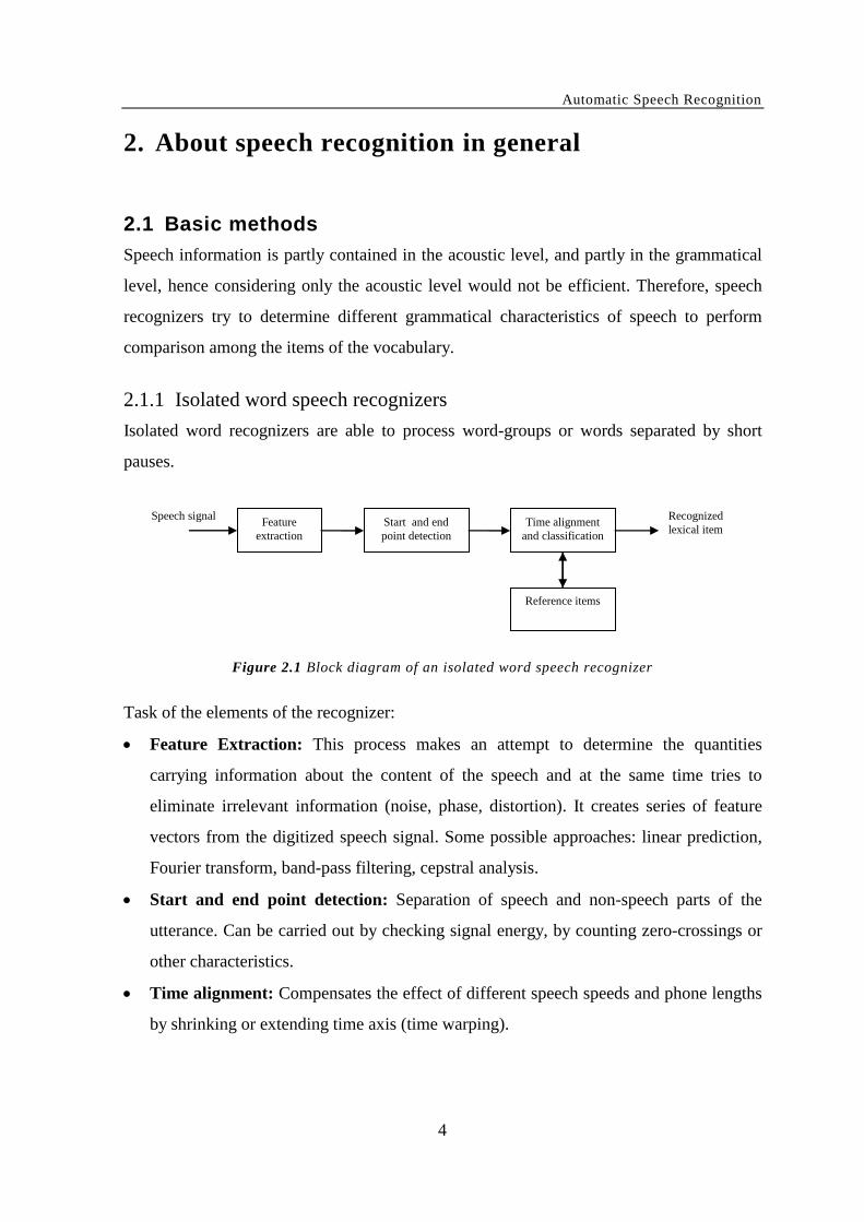
Figure 2.1 Block diagram of an isolated word speech recognizer

Task of the elements of the recognizer:

Feature Extraction: This process makes an attempt to determine the quantities

carrying information about the content of the speech and at the same time tries to

eliminate irrelevant information (noise, phase, distortion). It creates series of feature

vectors from the digitized speech signal. Some possible approaches: linear prediction,

Fourier transform, band-pass filtering, cepstral analysis.

Start and end point detection: Separation of speech and non-speech parts of the

utterance. Can be carried out by checking signal energy, by counting zero-crossings or

other characteristics.

Time alignment: Compensates the effect of different speech speeds and phone lengths

by shrinking or extending time axis (time warping).

Recognized

lexical item

Speech signal Feature

extraction

Start and end

point detection

Time alignment

and classification

Reference items


5

Classification: Selects a reference item having feature vectors series that is the most

close to the feature vector series of the utterance. Distance can be measured by using

some kind of metrics (e.g. Euclidean distance)

The above described steps are usually referred to as Dynamic Time Warping (DTW)

technique. DTW-based recognizers are speaker dependent (every reference item has to be

trained with the user’s voice), and their lexicon size usually under 100 items. However, the

content of the lexicon in the most cases is not fixed; it can be edited by the user.

2.1.2 Continuous speech recognition

Nowadays for continuous speech recognition purposes almost exclusively Hidden Markov

Model (HMM) based systems are used. In this model, words and sentences are built up

from phone-level based HMM models. The incoming feature vector series – provided by

the feature extractor module – are evaluated with the so-called Viterbi algorithm to

determine the probability of each HMM state. After phone-based probabilities are

calculated the so-called pronunciation model helps to move up from level of phones to the

level of words. Continuous speech recognizers are commonly supported by word-based

grammars that contain probability weights for the connection of every lexical item.

Continuous speech recognizers work efficiently if the recognition task has limited

vocabulary and grammar. Hence e.g. medical dictation systems perform exceptionally well,

whereas recognition of spontaneous speech is still a major challenge. The HMM-based

method has the advantage over DTW, that it is performs much better for speaker

independent tasks. However DTW is language independent method and can be a better

choice for small vocabulary, speaker dependent solutions. HMM-based recognizers need to

be trained with large quantity (hundreds of hours) of speech, while DTW is manually

trained by user by uttering the lexical items.


6

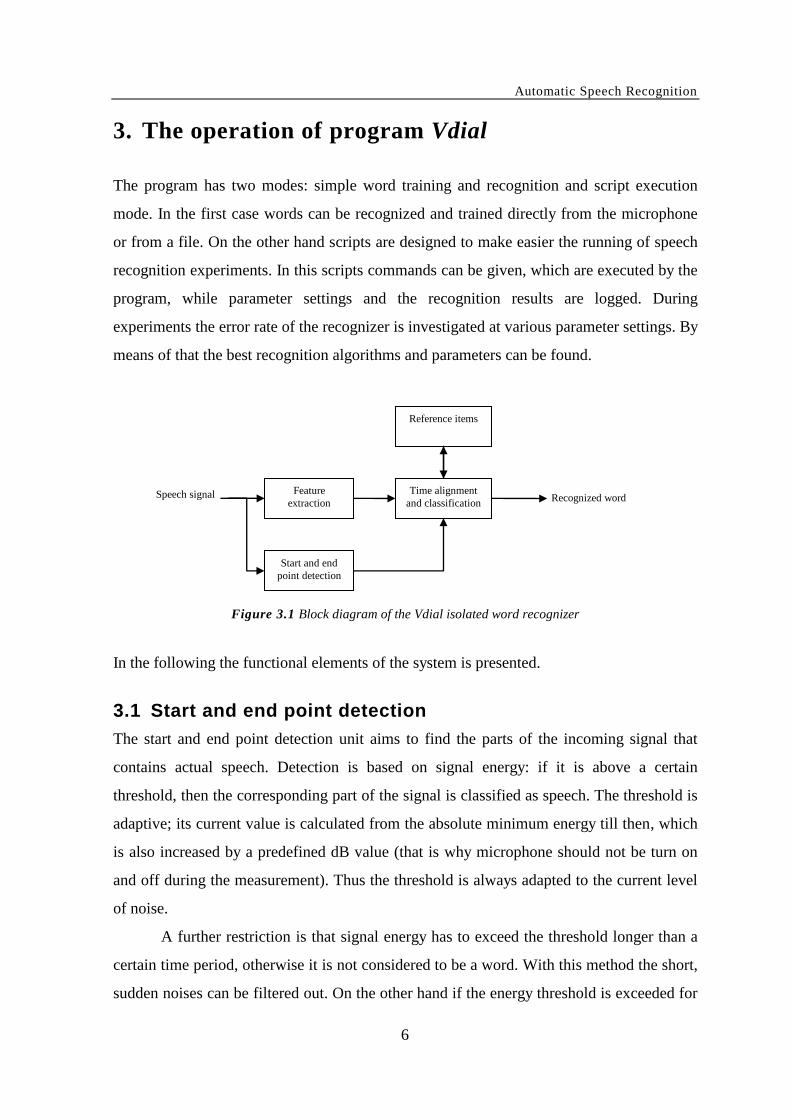
3. The operation of program Vdial

The program has two modes: simple word training and recognition and script execution

mode. In the first case words can be recognized and trained directly from the microphone

or from a file. On the other hand scripts are designed to make easier the running of speech

recognition experiments. In this scripts commands can be given, which are executed by the

program, while parameter settings and the recognition results are logged. During

experiments the error rate of the recognizer is investigated at various parameter settings. By

means of that the best recognition algorithms and parameters can be found.

Figure 3.1 Block diagram of the Vdial isolated word recognizer

In the following the functional elements of the system is presented.

3.1 Start and end point detection

The start and end point detection unit aims to find the parts of the incoming signal that

contains actual speech. Detection is based on signal energy: if it is above a certain

threshold, then the corresponding part of the signal is classified as speech. The threshold is

adaptive; its current value is calculated from the absolute minimum energy till then, which

is also increased by a predefined dB value (that is why microphone should not be turn on

and off during the measurement). Thus the threshold is always adapted to the current level

of noise.

A further restriction is that signal energy has to exceed the threshold longer than a

certain time period, otherwise it is not considered to be a word. With this method the short,

sudden noises can be filtered out. On the other hand if the energy threshold is exceeded for

Recognized word Speech signal Feature

extraction

Time alignment

and classification

Reference items

Start and end

point detection


7

too long (longer than a given time period), the given piece of signal is rejected to be part of

speech in order to avoid any long-term source of noise disturbs the system. Besides, these

long, large volume parts are used to refine the threshold level. One additional important

aspect is that words containing short, inter-word silences should not be split into two parts.

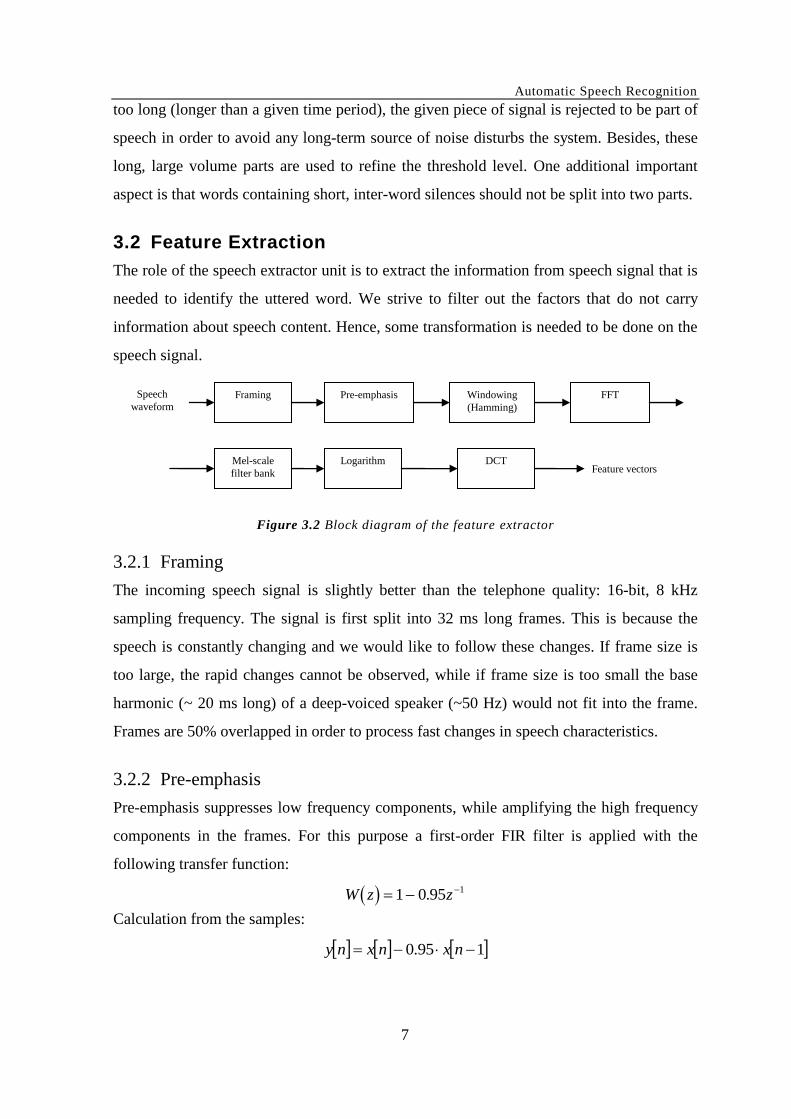
3.2 Feature Extraction

The role of the speech extractor unit is to extract the information from speech signal that is

needed to identify the uttered word. We strive to filter out the factors that do not carry

information about speech content. Hence, some transformation is needed to be done on the

speech signal.

Figure 3.2 Block diagram of the feature extractor

3.2.1 Framing

The incoming speech signal is slightly better than the telephone quality: 16-bit, 8 kHz

sampling frequency. The signal is first split into 32 ms long frames. This is because the

speech is constantly changing and we would like to follow these changes. If frame size is

too large, the rapid changes cannot be observed, while if frame size is too small the base

harmonic (~ 20 ms long) of a deep-voiced speaker (~50 Hz) would not fit into the frame.

Frames are 50% overlapped in order to process fast changes in speech characteristics.

3.2.2 Pre-emphasis

Pre-emphasis suppresses low frequency components, while amplifying the high frequency

components in the frames. For this purpose a first-order FIR filter is applied with the

following transfer function:

W z z 1 0 95 1.

Calculation from the samples:

195.0 nxnxny

Feature vectors

Framing Pre-emphasis Windowing

(Hamming)

FFT Speech

waveform

Mel-scale

filter bank

Logarithm DCT


8

3.2.3 Hamming-window

Before discrete Fourier transform (DFT) is performed, the signal has to be windowed, since

speech is not a perfectly periodic signal. The simplest, rectangular window spreads the

spectrum, thus it is not suitable for our purposes. However, by using Hamming window,

spectrum can be sharpened. Multiplication with the window function in the time domain

corresponds to convolution with the Fourier transform of the window function in the

frequency domain. So, the windowing of the signal can be interpreted as filtering of the

signal spectrum.

Function of the Hamming window:

h nn

N 0 54 0 46

2. . cos

where n = 0 ... N-1, and N is the window size.

3.2.4 Discrete Fourier transform

By applying discrete Fourier transform we can switch over from time to frequency domain.

This is necessary because factors charactering speech can only be observed in the spectrum.

In addition, many distortions in the input signal e.g. random phase shift, additive noise and

distortion (convolutional noise) can only be removed in frequency domain.

DFT is computed with the fast algorithm (FFT), because it is incomparably faster

than simple DFT algorithm. Only the square of the absolute value of the resulting complex

spectrum is further processed, phase information is irrelevant to the content of speech, thus

it is omitted. Calculation of DFT components:

F x i ek

i

Nj i k

0

12

where x[i] is the signal function in time domain, N is the size of transformation, while Fk-s

are the Fourier coefficients (k = 0 ... N-1, in our case k = 0…N/2-1).

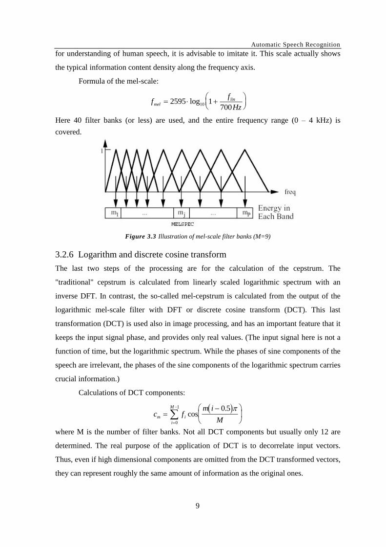
3.2.5 Mel-scale filter banks

The sensitivity of human sound perception varies in the function of the frequency. At

higher frequencies only larger distances in frequency can be distinguished than at lower

frequency. This distinctive ability (frequency resolution) under 1000 Hz changes

approximately linearly, while over it logarithmically (thus above 1000 Hz width of bands

increases exponentially). This is called the mel-scale. Since human hearing performs well


9

for understanding of human speech, it is advisable to imitate it. This scale actually shows

the typical information content density along the frequency axis.

Formula of the mel-scale:

ff

Hzmel

lin

2595 1

70010log

Here 40 filter banks (or less) are used, and the entire frequency range (0 – 4 kHz) is

covered.

Figure 3.3 Illustration of mel-scale filter banks (M=9)

3.2.6 Logarithm and discrete cosine transform

The last two steps of the processing are for the calculation of the cepstrum. The

"traditional" cepstrum is calculated from linearly scaled logarithmic spectrum with an

inverse DFT. In contrast, the so-called mel-cepstrum is calculated from the output of the

logarithmic mel-scale filter with DFT or discrete cosine transform (DCT). This last

transformation (DCT) is used also in image processing, and has an important feature that it

keeps the input signal phase, and provides only real values. (The input signal here is not a

function of time, but the logarithmic spectrum. While the phases of sine components of the

speech are irrelevant, the phases of the sine components of the logarithmic spectrum carries

crucial information.)

Calculations of DCT components:

c f

m i

Mm i

i

M

0

1 0 5cos

.

where M is the number of filter banks. Not all DCT components but usually only 12 are

determined. The real purpose of the application of DCT is to decorrelate input vectors.

Thus, even if high dimensional components are omitted from the DCT transformed vectors,

they can represent roughly the same amount of information as the original ones.


10

3.3 Time alignment and classification

The time alignment and classification unit takes the distance between the feature vector

series of the utterance and all the stored vector series. The result of the recognition is the

label of that stored vector series that is closest to the utterance. Time alignment here is

performed with the Dynamic Time Warping (DTW) algorithm.

The inputs of dynamic time warping are two vector series, while the output is the

aggregated distance between them. To solve the task we can draw up a coordinate system

in which the two axes show (discrete) time belongs to the compared vector series, while

grid points contain distance of the corresponding two vectors. As a metric for distance

Euclidean distance is used:

d x y x yk k

k

N

( , )

1

2

Figure 3.4 Linear time warping for two vectors with different length

In figure 3.4 the thick line indicates the path along which the incoming vector is uniformly

shrunk or extended for the comparison. This is called linear time warping. Stepping out on

the shaded area means some part of the vector is unevenly extended compared to other

parts. Actually this is the commonly good approach, because changes in length are usually

spread unevenly across the vector. For instance, in most languages if a word is pronounced

longer the expansion of vowels is relatively higher than the expansion of the consonants.

Therefore the path of the warping is usually not the diagonal. (Fig. 3.5.)


11

Figure 3.5 Time alignment along a curved path

However the path of time warping cannot be arbitrary. It is not allowed to go

backwards. In addition, the forward progress also can be restricted in various ways

depending on how much variation we allow during the process. Fig. 3.6 presents a few

options. In our system, the first one is used.

Figure 3.6 Some local continuity restrictions and the corresponding paths

To define the optimal route, some notations have to be introduced! Denote the time

warping functions with x and y, which create a relationship between ix and iy indices of

the vector series and between k discrete time.


12

x (k) = ix k = 1, 2, ..., T

and

y (k) = iy k = 1, 2, ..., T

where T is the normalized length of the two vector series. If a valid x and y pair is

denoted with = (x, y), then a global distance between the vector series for a given is

the following:

d X Y d k kX Y

k

T

( , ) ,

1

Therefore distance between X and Y can be defined as:

d X Y d X Y, : min ,

where has to meet certain conditions:

- starting point: x (1) = 1 y (1) = 1

- end: x (T) = Tx y (T) = Ty

- monotony: x (k+1) x (k) y (k+1) y (k)

- local continuity: x (k+1) - x (k) 1 y (k+1) - y (k) 1.

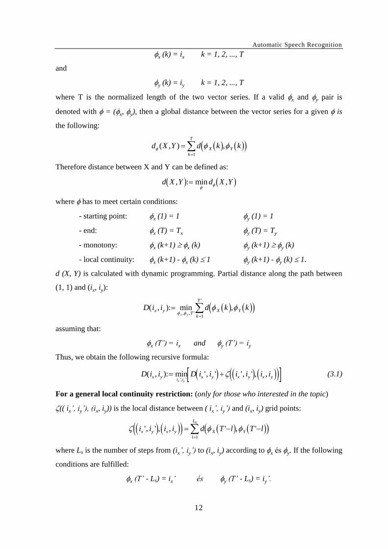
d (X, Y) is calculated with dynamic programming. Partial distance along the path between

(1, 1) and (ix, iy):

D i i d k kx yT

X Y

k

T

x y

( , ): min ,, , '

'

1

assuming that:

x (T’) = ix and y (T’) = iy

Thus, we obtain the following recursive formula:

D i i D i i i i i ix yi i

x y x y x yx y

( , ): min ', ' ', ' , ,', '

(3.1)

For a general local continuity restriction: (only for those who interested in the topic)

(( ix’, iy’), (ix, iy)) is the local distance between ( ix’, iy’) and (ix, iy) grid points:

i i i i d T l T lx y x y X Y

l

LS

', ' , , ' , '

1

where Ls is the number of steps from (ix’, iy’) to (ix, iy) according to x és y. If the following

conditions are fulfilled:

x (T’ - Ls) = ix’ és y (T’ - Ls) = iy’.


13

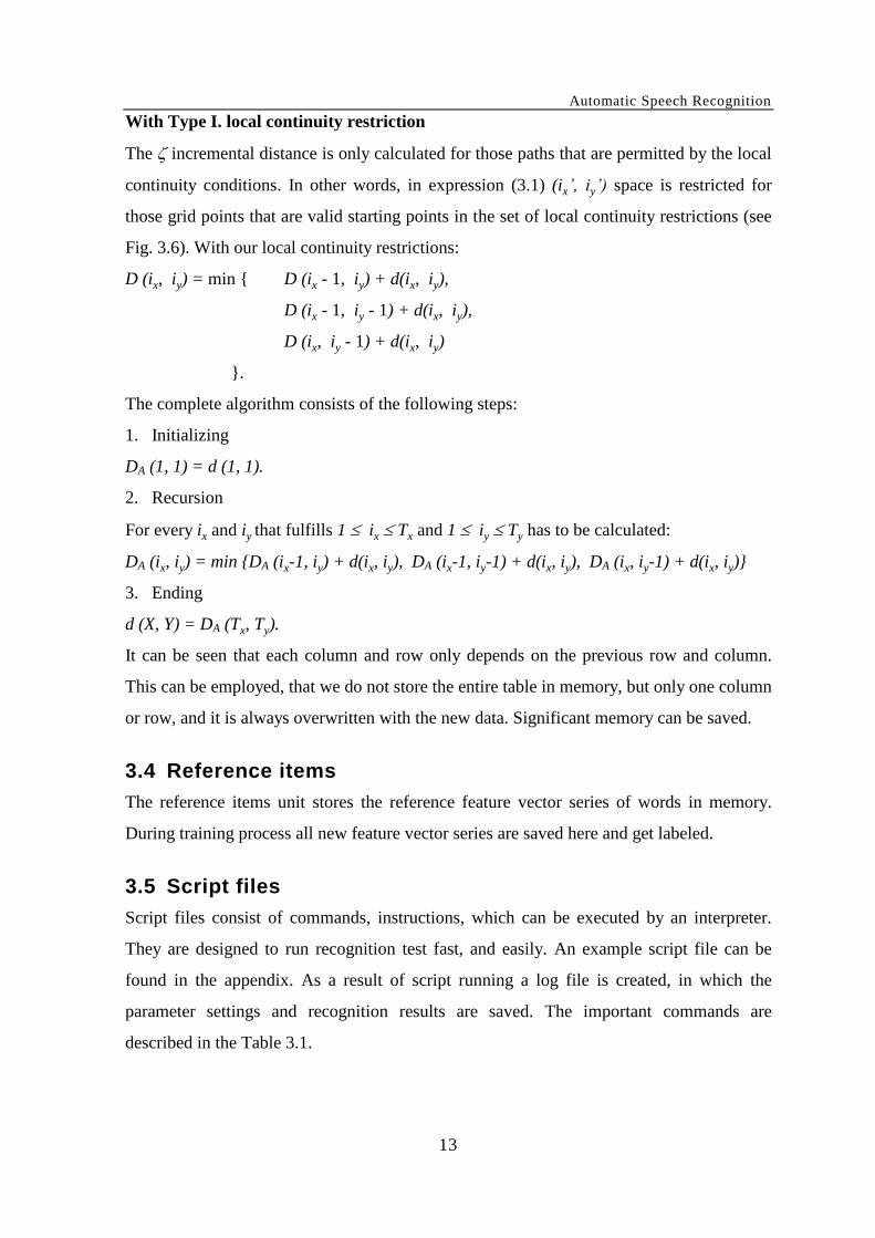
With Type I. local continuity restriction

The incremental distance is only calculated for those paths that are permitted by the local

continuity conditions. In other words, in expression (3.1) (ix’, iy’) space is restricted for

those grid points that are valid starting points in the set of local continuity restrictions (see

Fig. 3.6). With our local continuity restrictions:

D (ix, iy) = min { D (ix - 1, iy) + d(ix, iy),

D (ix - 1, iy - 1) + d(ix, iy),

D (ix, iy - 1) + d(ix, iy)

}.

The complete algorithm consists of the following steps:

1. Initializing

DA (1, 1) = d (1, 1).

2. Recursion

For every ix and iy that fulfills 1 ix Tx and 1 iy Ty has to be calculated:

DA (ix, iy) = min {DA (ix-1, iy) + d(ix, iy), DA (ix-1, iy-1) + d(ix, iy), DA (ix, iy-1) + d(ix, iy)}

3. Ending

d (X, Y) = DA (Tx, Ty).

It can be seen that each column and row only depends on the previous row and column.

This can be employed, that we do not store the entire table in memory, but only one column

or row, and it is always overwritten with the new data. Significant memory can be saved.

3.4 Reference items

The reference items unit stores the reference feature vector series of words in memory.

During training process all new feature vector series are saved here and get labeled.

3.5 Script files

Script files consist of commands, instructions, which can be executed by an interpreter.

They are designed to run recognition test fast, and easily. An example script file can be

found in the appendix. As a result of script running a log file is created, in which the

parameter settings and recognition results are saved. The important commands are

described in the Table 3.1.


14

Command Parameters What it does

Train WAVE files

separated by space

Read files from the input, searches for words in them,

performs feature extraction, and stores the feature vector

series into the word database

TrainFromMic – Does the same as the previous command, but it trains the

system from microphone

Test WAVE files

separated by space

Read every file step by step, performs word recognition in

them (searches for the closest reference file), and returns the

recognized strings

Play a WAVE file Plays back the given sound file

Rem optional text After this command comments can be written which are

ignored by the interpreter

Stop – The script execution stops

Call name of a procedure Calls a procedure

Proc name of a procedure Marks the beginning of a procedure

EndProc – Marks the end of a procedure

Echo optional text Everything written after this command is sent to the log file

ForgetTemplates – Delete the content of word database

ClearStatistics – Delete all statistics

ShowStatistics – Statistical data is sent to the log file

Set Path path Path for the wave files can be given

Set VectorType FilterBank or

MelCep

Type of feature extraction can be modified

Set FilterBankSize an integer Number of filter banks can be modified. If VectorType=

FilterBank, then this number also gives the dimension of the

feature vector. If VectorType= MelCep then is gives the

dimension of the vectors entering into cepstrum processing

Set MelCepSize an integer Order of mel-cepstrum processing can be modified. If

VectorType= FilterBank then this command is ignored

Table 3.1. Instruction set


15

4. The usage of program Vdial

4.1 Menus

4.1.1 Templates menu

By using this menu items content of word database can be saved to disk, loaded from disk

or deleted.

4.1.2 Run menu

Selecting Analyze from mic menu item the program performs feature extraction on

microphone signal, and tries to find word boundaries

Analyze file... menu item similar to the previous one, but it operates on wave files

Train from mic command stores all the words in the word database that we label in the

utterance. A label can be designated to more than one utterance.

Train file... command works on a chosen wave file. A description file has to be

attached! (see below)

Recognize from mic performs recognition on the signal gave to the microphone

Recognize file... performs speech recognition from sound file. If a description file is

attached, then it goes through the words step by steps and compares them to the

recognized strings. Thus recognition statistics can be made.

Run command file... runs a script file

4.1.3 Options menu

if Step by step item is active, the program only calculates if space button is pressed, if it

is engaged calculation hangs up

if Word by word item is active, the program goes performs recognition word by word

Do next frame substitutes space button in step by step mode

Do next word substitutes space button in word by word mode

Pause item hangs up calculation if step by step or word by word mode is not active

Stop hangs up the currently running calculation. Same as pressing Escape button

if Playback item is active, the program plays back the sound files after every processing


16

Isolated word recognition, Connected word recognition, Continuous recognition

The latter two is only experimentally realized here.

4.1.4 Settings menu

Find word settings: parameters of word search can be modified here

Signal processing settings: sampling frequency, the parameters of feature extraction,

type of feature vectors and additive noise related parameters can be set here

Plot settings: features of the plotted functions can be modified

4.2 Description files

Description file is a text file (TXT extension) that has to be stored next to wave file having

the same name as the wave file. It contains words separated by space or new line character

that was uttered in the recorded audio file.


17

5. Appendix

5.1 A script file and its output TEST1.CMD:

ClearTemplates

Set VectorType = FilterBank

Set FilterBankSize = 8

Call Test12


Call Test12


Call Test12


Call Test12

Set VectorType = MelCep

Set MelCepSize = 8


Call Test12


Call Test12


Call Test12


Call Test12

Set MelCepSize = 12


Call Test12


Call Test12


Call Test12


Call Test12

Stop

Proc Test12

Call Test1

Call Test2

EndProc

Proc Test1

Set Path = WAVES\SZAMOK

ClearStatistics

Echo Train files: lb1 - lb4, test files: lb1 - lb4

ClearTemplates

Train lb1

Test lb2 lb3 lb4

ClearTemplates

Train lb2

Test lb1 lb3 lb4

ClearTemplates

Train lb3

Test lb1 lb2 lb4

ClearTemplates

Train lb4

Test lb1 lb2 lb3

ShowStatistics

ClearStatistics


ClearTemplates

Train lb5

Test lb6 lb7 lb8

ClearTemplates

Train lb6

Test lb5 lb7 lb8

ClearTemplates

Train lb7

Test lb5 lb6 lb8

ClearTemplates

Train lb8

Test lb5 lb6 lb7

ShowStatistics

ClearStatistics


ClearTemplates

Train lb9

Test lb10 lb11 lb12

ClearTemplates

Train lb10

Test lb9 lb11 lb12

ClearTemplates

Train lb11

Test lb9 lb10 lb12

ClearTemplates

Train lb12

Test lb9 lb10 lb11

ShowStatistics

Echo

ClearTemplates

EndProc

Proc Test2

Set Path = WAVES\SZAMOK

ClearStatistics


ClearTemplates

Train lb1

Test lb2 lb3 lb4 lb5 lb6 lb7 lb8 lb9 lb10 lb11 lb12

ClearTemplates

Train lb2


ClearTemplates

Train lb3


ClearTemplates

Train lb4


ShowStatistics

ClearStatistics


ClearTemplates

Train lb5


ClearTemplates

Train lb6


ClearTemplates

Train lb7


ClearTemplates

Train lb8


ShowStatistics

ClearStatistics


ClearTemplates

Train lb9


ClearTemplates

Train lb10


ClearTemplates

Train lb11


ClearTemplates

Train lb12


ShowStatistics

Echo

ClearTemplates

EndProc


18

TEST1.LOG:

Project OVSR - CMD Log file

VectorType = FilterBank

FilterBankSize = 8

Train files: lb1 - lb4, test files: lb1 - lb4

Word error rate: 2% (3 of 120)











FilterBankSize = 12













FilterBankSize = 20













FilterBankSize = 30













VectorType = MelCep

MelCepSize = 8

FilterBankSize = 8













FilterBankSize = 12













FilterBankSize = 20













FilterBankSize = 30













MelCepSize = 12

FilterBankSize = 8













FilterBankSize = 12













FilterBankSize = 20













FilterBankSize = 30













Date post:	15-Mar-2018
Category:	Documents
Upload:	vankhuong
View:	219 times
Download:	2 times

Automatic Speech Recognition - alpha.tmit.bme.hualpha.tmit.bme.hu/meresek/ttmer16a_eng.pdf · After...

Documents