Instructor: Preethi Jyothi Jan 23, 2017

Automatic Speech Recognition (CS753)Lecture 7: Hidden Markov Models (Part III)Automatic Speech Recognition (CS753)

AcousticFeatures

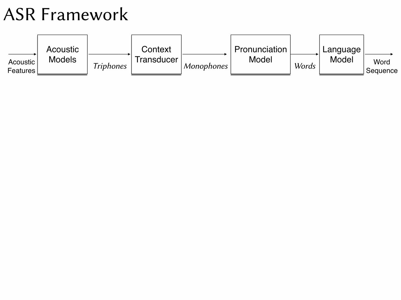
ASR Framework

Language Model Word

Sequence

AcousticModels

Triphones

ContextTransducer

Monophones

Pronunciation Model

Words

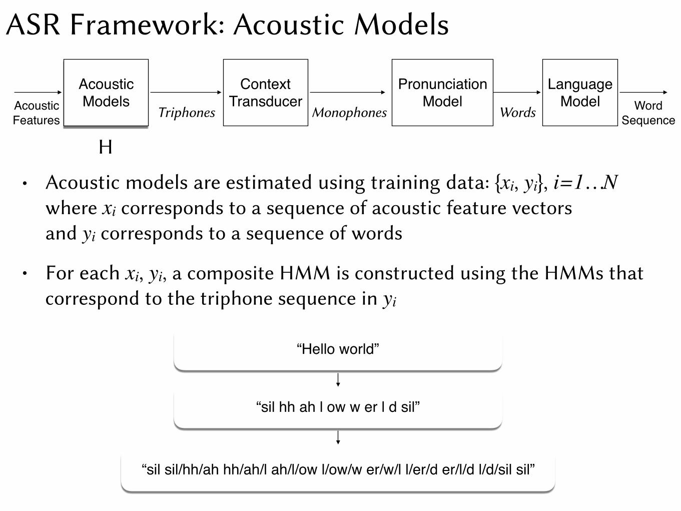
ASR Framework: Acoustic Models

AcousticFeatures

Language Model Word

Sequence

AcousticModels

Triphones

ContextTransducer

Monophones

Pronunciation Model

Words

H

• Acoustic models are estimated using training data: {xi, yi}, i=1…Nwhere xi corresponds to a sequence of acoustic feature vectorsand yi corresponds to a sequence of words

“Hello world”

“sil hh ah l ow w er l d sil”

“sil sil/hh/ah hh/ah/l ah/l/ow l/ow/w er/w/l l/er/d er/l/d l/d/sil sil”

• For each xi, yi, a composite HMM is constructed using the HMMs that correspond to the triphone sequence in yi

ASR Framework: Acoustic Models

AcousticFeatures

Language Model Word

Sequence

AcousticModels

Triphones

ContextTransducer

Monophones

Pronunciation Model

Words

H

• Acoustic models are estimated using training data: {xi, yi}, i=1…Nwhere xi corresponds to a sequence of acoustic feature vectorsand yi corresponds to a sequence of words

• For each xi, yi, a composite HMM is constructed using the HMMs that correspond to the triphone sequence in yi

• These parameters are fit to the acoustic data {xi}, i=1…N using the Baum-Welch algorithm (EM)

• Parameters of these composite HMMs are the parameters of the constituent triphone HMMs.

Parameter θ determines Pr(x, z; θ) where x is observed and z is hidden

Observed data: i.i.d samples xi, i=1, …, N

Goal: Find where

Initial parameters: θ0

Iteratively compute θl as follows:

Recall EM: Fitting Parameters to Data

Q(✓, ✓

`�1) =

NX

i=1

X

z

Pr(z|xi; ✓`�1

) log Pr(xi, z; ✓)

✓` = argmax

✓Q(✓, ✓`�1

)

L(✓) =NX

i=1

log Pr(xi; ✓)argmax

✓L(✓)

L(✓)� L(✓`�1) � Q(✓, ✓`�1)�Q(✓`�1, ✓`�1)

Estimate θl cannot get worse over iterations because for all θ:

EM is guaranteed to converge to a local optimum [Wu83]

Coin example to illustrate EM

Coin�1 Coin�2 Coin�3

𝜌1 = Pr(H) = 0.3 𝜌2 = Pr(H) = 0.4 𝜌3 = Pr(H) = 0.6

The following sequence is observed: “HH, TT, HH, TT, HH”

How do you estimate 𝜌1, 𝜌2 and 𝜌3?

Toss Coin�1�privately if it shows H: Toss Coin�2 twiceelse Toss Coin�3 twice

Repeat:

Coin example to illustrate EM

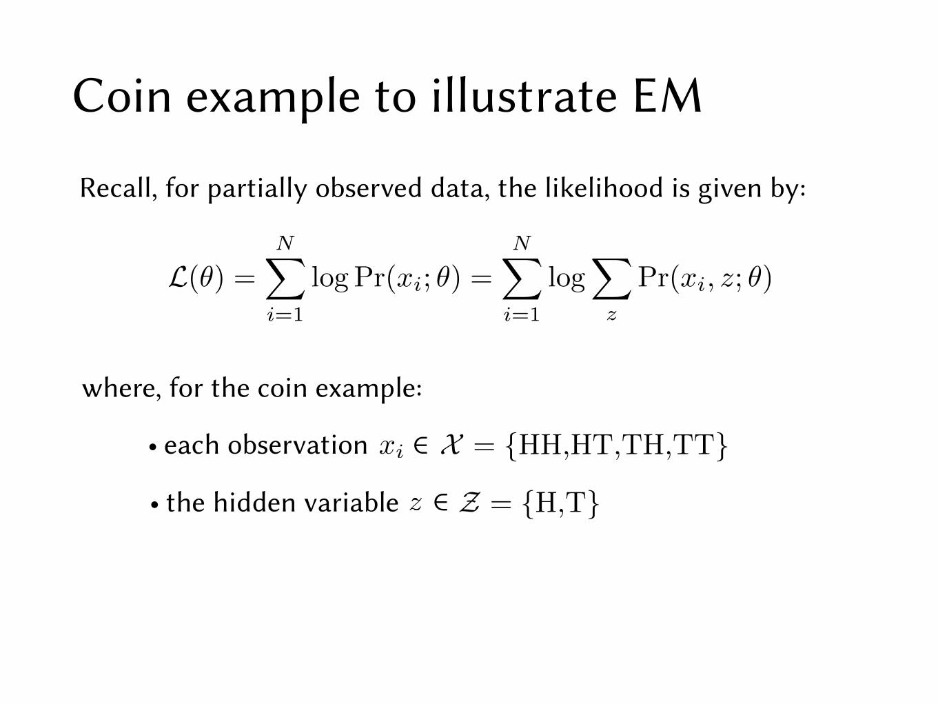
Recall, for partially observed data, the likelihood is given by:

∈ • each observation xi

where, for the coin example:

• the hidden variable ∈z

X = {HH,HT,TH,TT}

Z = {H,T}

L(✓) =NX

i=1

log Pr(xi; ✓) =

NX

i=1

log

X

z

Pr(xi, z; ✓)

Coin example to illustrate EM

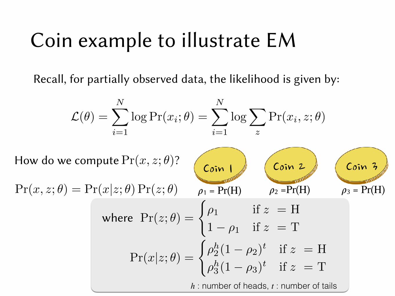
Recall, for partially observed data, the likelihood is given by:

Pr(x, z; ✓) = Pr(x|z; ✓) Pr(z; ✓)

How do we compute ?Pr(x, z; ✓)

where Pr(z; ✓) =

(⇢1 if z = H

1� ⇢1 if z = T

Coin�1𝜌1 = Pr(H)

Coin�2 Coin�3

𝜌2 =Pr(H) 𝜌3 = Pr(H)

L(✓) =NX

i=1

log Pr(xi; ✓) =

NX

i=1

log

X

z

Pr(xi, z; ✓)

h : number of heads, t : number of tails

Pr(x|z; ✓) =(⇢

h2 (1� ⇢2)

t if z = H

⇢

h3 (1� ⇢3)

t if z = T

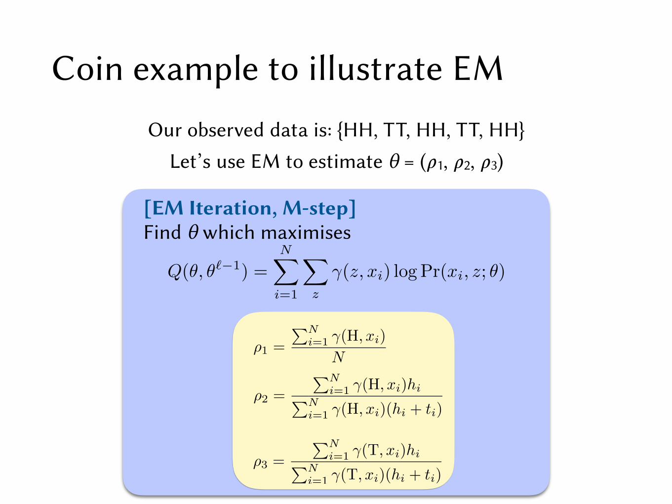
Our observed data is: {HH, TT, HH, TT, HH}

Let’s use EM to estimate θ = (𝜌1, 𝜌2, 𝜌3)

= 0.16= 0.49 What is 𝛾(H, TT)?

What is 𝛾(H, HH)?

Suppose θl -1 is 𝜌1 = 0.3, 𝜌2 = 0.4, 𝜌3 = 0.6:

[EM Iteration, E-step]Compute quantities involved in

where 𝛾(z, x) = Pr(z | x ;θl -1)

Q(✓, ✓

`�1) =

NX

i=1

X

z

�(z, xi) log Pr(xi, z; ✓)

Coin example to illustrate EM

i.e., compute 𝛾(z, xi) for all z and all i

Our observed data is: {HH, TT, HH, TT, HH}

[EM Iteration, M-step]Find θ which maximises

Q(✓, ✓

`�1) =

NX

i=1

X

z

�(z, xi) log Pr(xi, z; ✓)

Coin example to illustrate EM

⇢2 =

PNi=1 �(H, xi)hiPN

i=1 �(H, xi)(hi + ti)

⇢1 =

PNi=1 �(H, xi)

N

⇢3 =

PNi=1 �(T, xi)hiPN

i=1 �(T, xi)(hi + ti)

Let’s use EM to estimate θ = (𝜌1, 𝜌2, 𝜌3)

Coin example to illustrate EM

This was a very simple HMM (with observations from 3 steps)

State remains the same after the first transition

γ estimated the distribution of this state

More generally, will need the distribution of the state and the transition at each time step

EM for general HMMs: Baum-Welch algorithm (1972) predates the general formulation of EM (1977)

H

T

ε/𝜌1

ε/1-𝜌1

H/𝜌2

T/1-𝜌2

H/𝜌3

T/1-𝜌3

Observed data: N sequences, xi = (xi1, …, xiTi), i=1…N where xit ∈ ℝd

Parameters θ : transition matrix A, observation probabilities B

[EM Iteration, E-step]Compute quantities involved in Q(θ,θl -1) 𝛾i,t (j) = Pr(zt = j | xi ;θl -1) 𝛏i,t(j,k) = Pr(zt-1 = j, zt = k | xi ;θl -1)

Baum-Welch Algorithm as EM

Parameters θ : transition matrix A, observation probabilities B

[EM Iteration, M-step]Find θ which maximises Q(θ,θl -1)

Baum-Welch Algorithm as EM

Observed data: N sequences, xi = (xi1, …, xiTi), i=1…N where xit ∈ ℝd

Aj,k =

PNi=1

PTi

t=2 ⇠i,t(j, k)PNi=1

PTi

t=2

Pk0 ⇠i,t(j, k0)

Bj,v

=

PN

i=1

Pt:xit=v

�i,t

(j)P

N

i=1

PTi

t=1 �i,t(j)

Gaussian Observation Model• So far we considered HMMs with discrete outputs

• In acoustic models, HMMs output real valued vectors

• Hence, observation probabilities are defined using probability density functions

• A widely used model: Gaussian distribution

N (x|µ,�2) =1p2⇡�2

e

� 12�2 (x�µ)2

• HMM emission/observation probabilities bj(x) = 𝒩(x | µj, σj2)where µj is the mean associated with state j and σj2 is its variance.

• For multivariate Gaussians, bj(x) = 𝒩(x | µj, Σj) where Σ is the covariance associated with state j

BW for Gaussian Observation Model

Parameters θ : transition matrix A, observation prob. B = {(µj,Σj)} for all j

[EM Iteration, M-step]Find θ which maximises Q(θ,θl -1)

µj =

PNi=1

PTi

t=1 �i,t(j)xitPNi=1

PTi

t=1 �i,t(j)

⌃j =

PNi=1

PTi

t=1 �i,t(j)(xit � µj)(xit � µj)TPNi=1

PTi

t=1 �i,t(j)

A and π same as with discrete outputs

Observed data: N sequences, xi = (xi1, …, xiTi), i=1…N where xit ∈ ℝd

B = {(µj,Σj)} for all j

Gaussian Mixture Model• A single Gaussian observation model assumes that the

observed acoustic feature vectors are unimodal

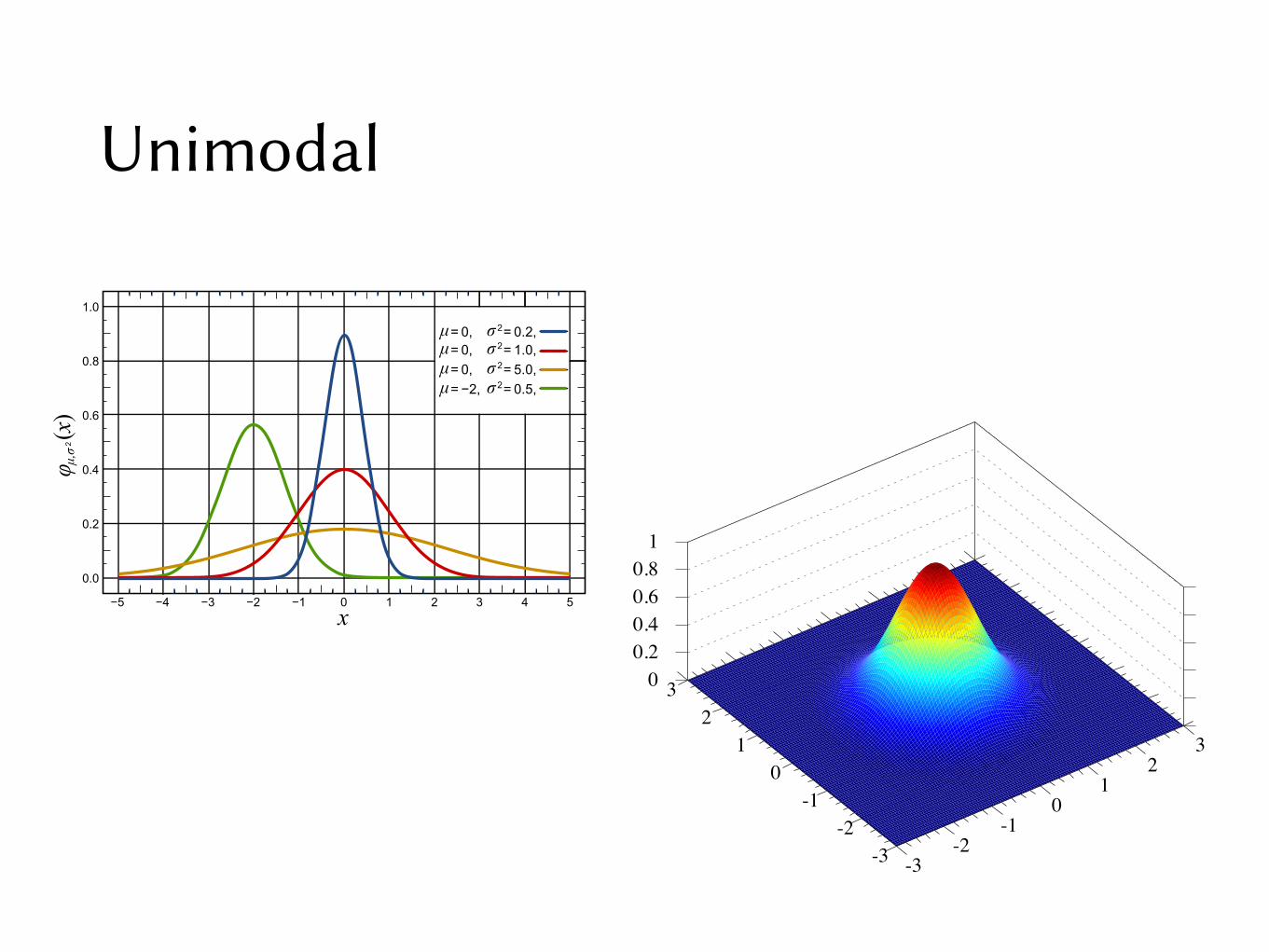
Unimodal

23/01/2017 https://upload.wikimedia.org/wikipedia/commons/7/74/Normal_Distribution_PDF.svg

https://upload.wikimedia.org/wikipedia/commons/7/74/Normal_Distribution_PDF.svg 1/1

φ μ,σ

2(

0.8

0.6

0.4

0.2

0.0

−5 −3 1 3 5x

1.0

−1 0 2 4−2−4

x)

0,μ=0,μ=0,μ=−2,μ=

2 0.2,σ =2 1.0,σ =2 5.0,σ =2 0.5,σ =

23/01/2017 Gnuplot

https://upload.wikimedia.org/wikipedia/commons/3/3e/Gaussian_2d.svg 1/1

-3-2

-10

12

3

-3-2

-10

12

300.20.40.60.81

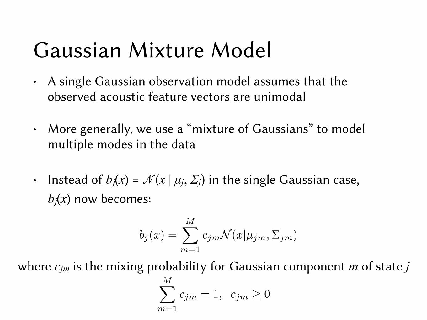
Gaussian Mixture Model• A single Gaussian observation model assumes that the

observed acoustic feature vectors are unimodal

• More generally, we use a “mixture of Gaussians” to model multiple modes in the data

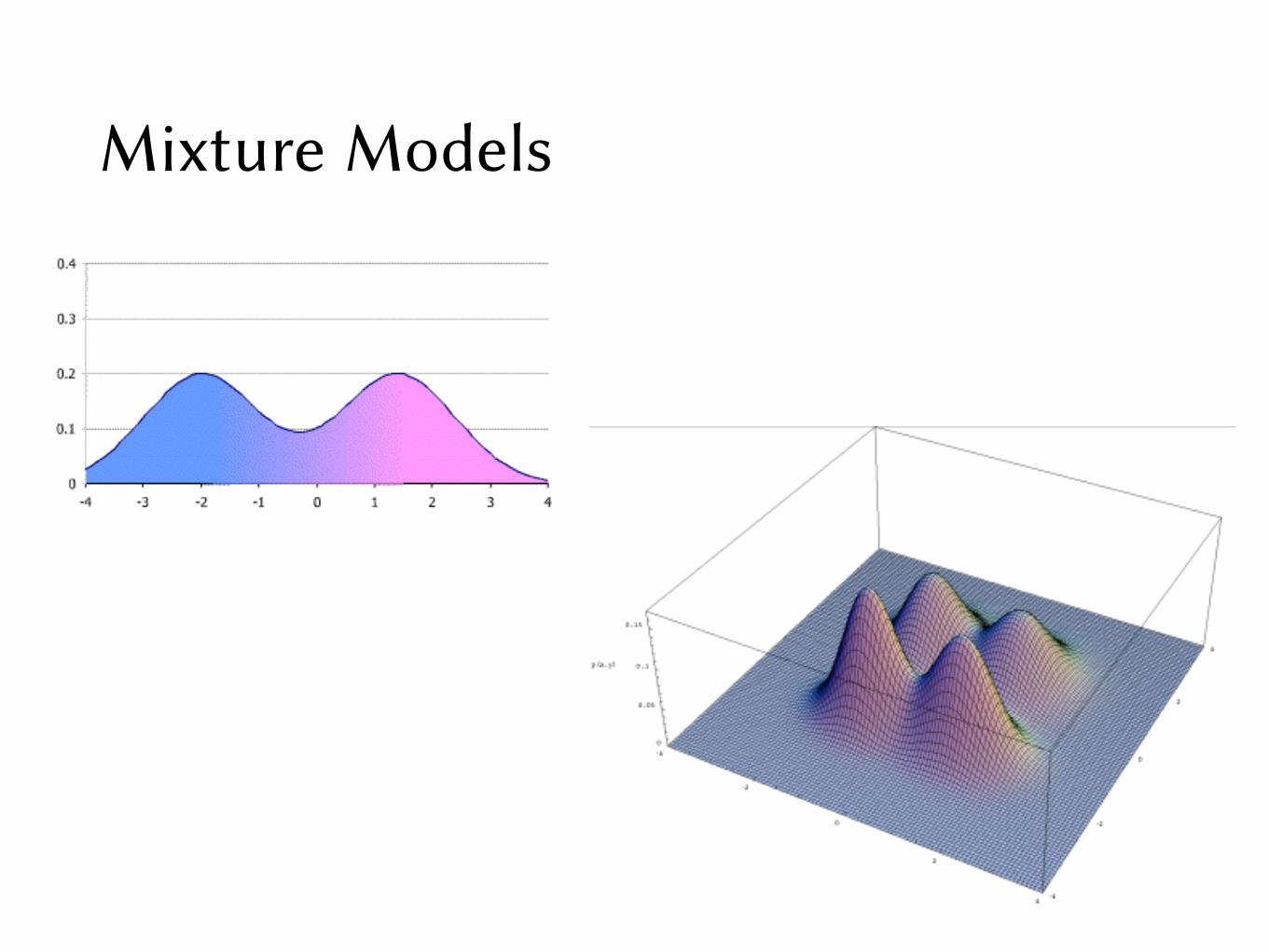
Mixture Models

Gaussian Mixture Model

• More generally, we use a “mixture of Gaussians” to model multiple modes in the data

• Instead of bj(x) = 𝒩(x | µj, Σj) in the single Gaussian case, bj(x) now becomes:

bj(x) =MX

m=1

cjmN (x|µjm,⌃jm)

where cjm is the mixing probability for Gaussian component m of state jMX

m=1

cjm = 1, cjm � 0

• A single Gaussian observation model assumes that the observed acoustic feature vectors are unimodal

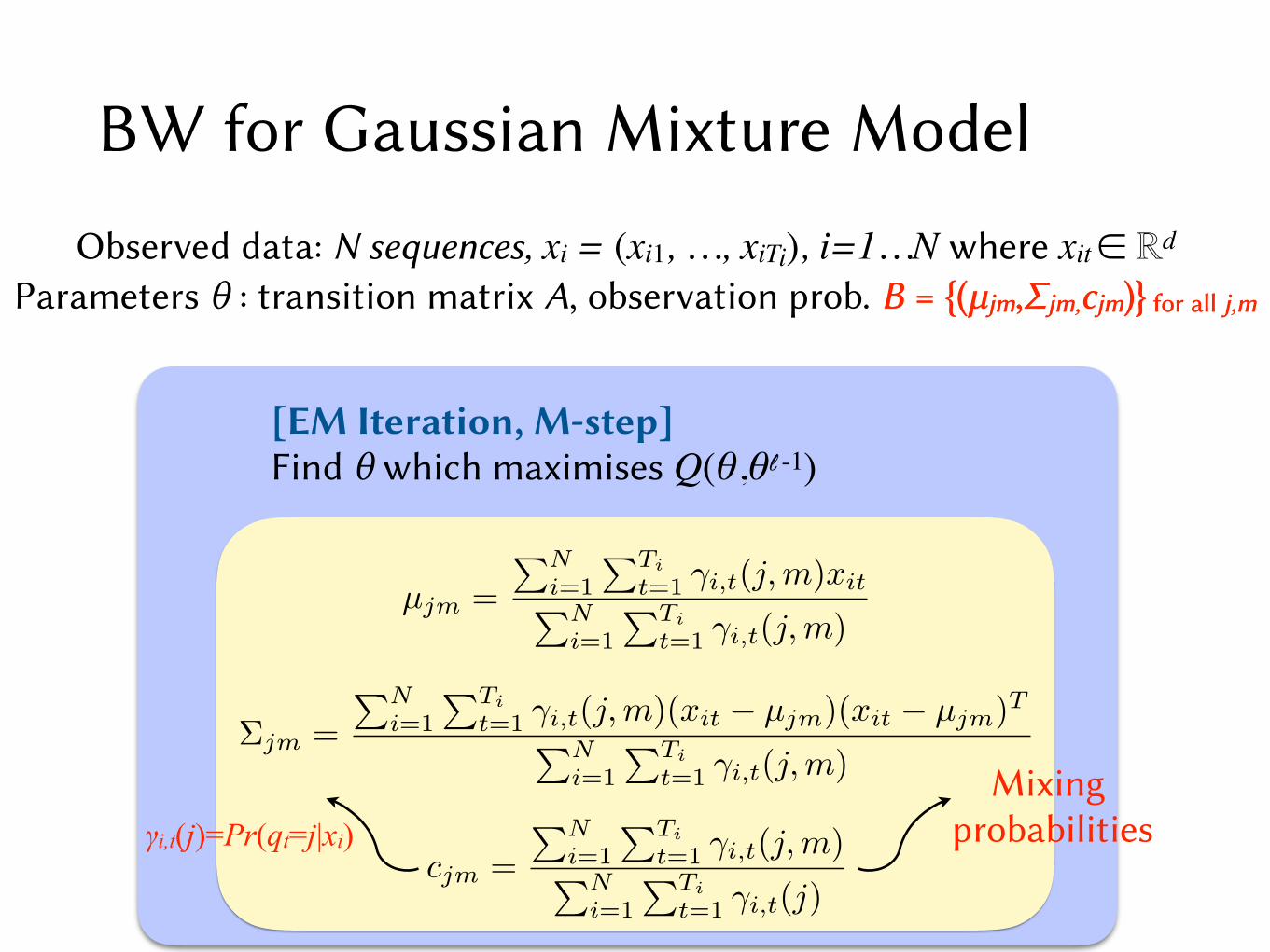
BW for Gaussian Mixture Model

Parameters θ : transition matrix A, observation prob. B = {(µjm,Σjm,cjm)} for all j,m

[EM Iteration, M-step]Find θ which maximises Q(θ,θl -1)

µjm =

PNi=1

PTi

t=1 �i,t(j,m)xitPNi=1

PTi

t=1 �i,t(j,m)

⌃jm =

PNi=1

PTi

t=1 �i,t(j,m)(xit � µjm)(xit � µjm)TPN

i=1

PTi

t=1 �i,t(j,m)

cjm =

PNi=1

PTi

t=1 �i,t(j,m)PN

i=1

PTi

t=1 �i,t(j)

Observed data: N sequences, xi = (xi1, …, xiTi), i=1…N where xit ∈ ℝd

Mixing probabilities

B = {(µjm,Σjm,cjm)} for all j,m

γi,t(j)=Pr(qt=j|xi)

Number of HMM-GMM Parameters

• Number of triphones that appear in data ≈ 1000s or 10,000s

• If each triphone HMM has 3 states and each state generates m-component GMMs (m ≈ 64), for d-dimensional acoustic feature vectors (d ≈ 40) with Σ having d2 parameters

• Results in millions of HMM-GMM parameters!

• How do we effectively estimate these parameters?

• One solution is “parameter tying” at the state level

Next class: Tied-state Triphone HMMs