Automatic Tuning of Data-Intensive Analytical Workloads by Herodotos Herodotou Department of Computer Science Duke University Date: Approved: Shivnath Babu, Supervisor Jun Yang Jeffrey Chase Christopher Olston Dissertation submitted in partial fulfillment of the requirements for the degree of Doctor of Philosophy in the Department of Computer Science in the Graduate School of Duke University 2012
Transcript
Automatic Tuning of Data-Intensive Analytical
Workloads
by
Herodotos Herodotou
Department of Computer ScienceDuke University
Date:Approved:
Shivnath Babu, Supervisor
Jun Yang
Jeffrey Chase
Christopher Olston
Dissertation submitted in partial fulfillment of the requirements for the degree ofDoctor of Philosophy in the Department of Computer Science
in the Graduate School of Duke University2012
Abstract
Automatic Tuning of Data-Intensive Analytical
Workloads
by
Herodotos Herodotou
Department of Computer ScienceDuke University
Date:Approved:
Shivnath Babu, Supervisor
Jun Yang
Jeffrey Chase
Christopher Olston
An abstract of a dissertation submitted in partial fulfillment of the requirements forthe degree of Doctor of Philosophy in the Department of Computer Science
4.5 A subset of job profile fields for two Word Co-occurrence jobs run withdifferent settings for io.sort.mb. . . . . . . . . . . . . . . . . . . . . . 52
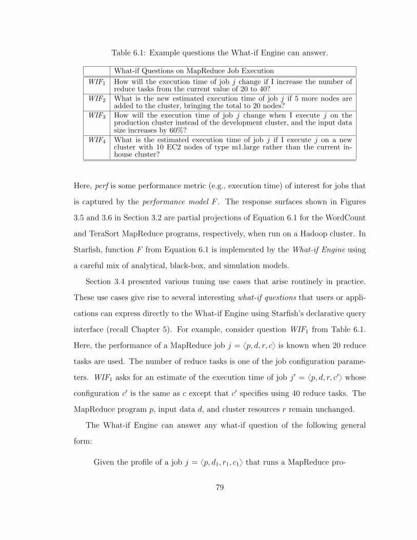
6.1 Example questions the What-if Engine can answer. . . . . . . . . . . 79
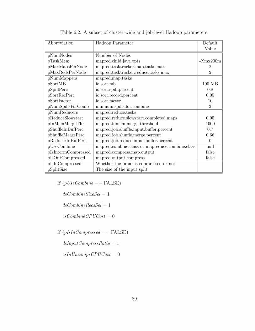
6.2 A subset of cluster-wide and job-level Hadoop parameters. . . . . . . 89
6.3 Cluster-wide Hadoop parameter settings for five EC2 node types. . . 111
6.4 MapReduce programs and corresponding datasets for the evaluationof the What-if Engine. . . . . . . . . . . . . . . . . . . . . . . . . . . 111
7.1 MapReduce programs and corresponding datasets for the evaluationof the Job Optimizer. . . . . . . . . . . . . . . . . . . . . . . . . . . . 134
7.2 MapReduce job configuration settings in Hadoop suggested by Rules-of-Thumb and the cost-based Job Optimizer for the Word Co-occurrenceprogram. . . . . . . . . . . . . . . . . . . . . . . . . . . . . . . . . . . 135
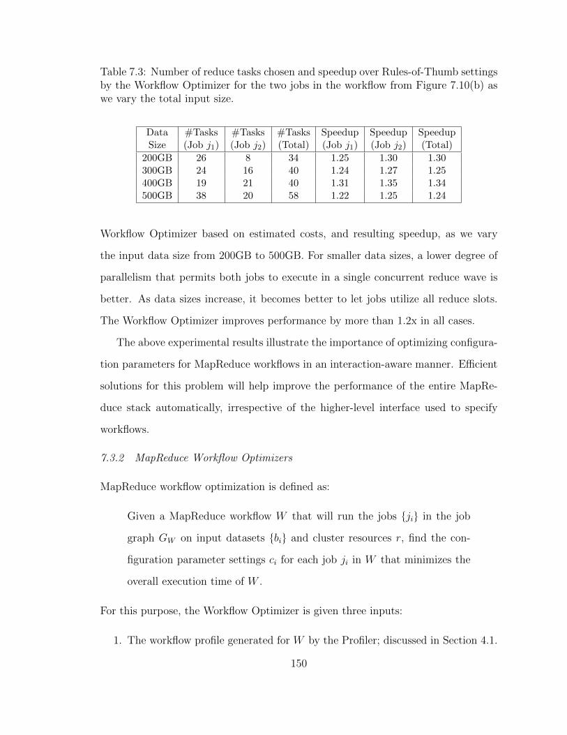
7.3 Number of reduce tasks chosen and speedup over Rules-of-Thumb set-tings by the Workflow Optimizer for a workflow as we vary the totalinput size. . . . . . . . . . . . . . . . . . . . . . . . . . . . . . . . . . 150
x
7.4 MapReduce workflows and corresponding dataset sizes on two clustersfor the evaluation of the Workflow Optimizer. . . . . . . . . . . . . . 160
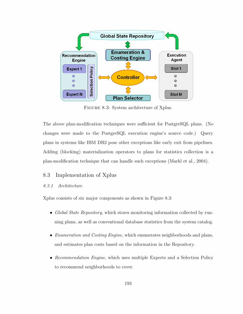
8.1 Properties of the current experts in Xplus. . . . . . . . . . . . . . . . 189
8.2 Comparison of Xplus, Leo, Pay-As-You-Go, and ATO. . . . . . . . . 199
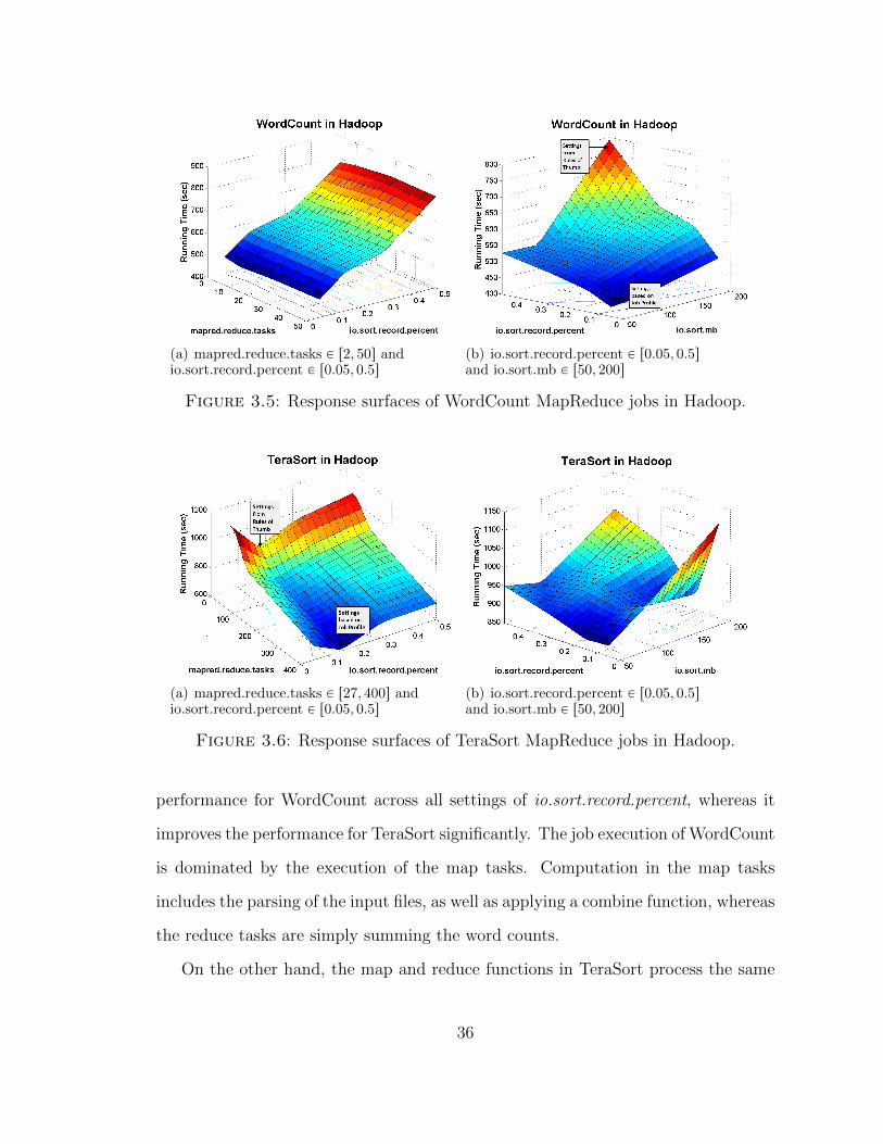
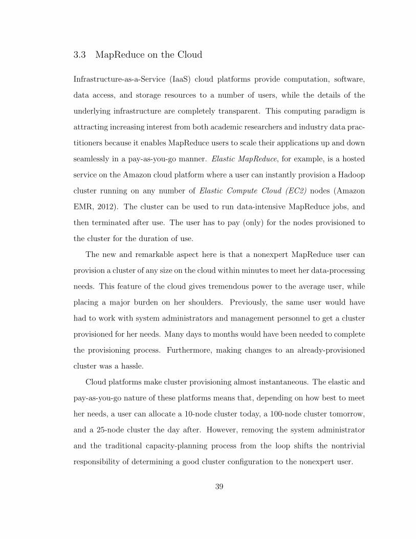
3.5 Response surfaces of WordCount MapReduce jobs in Hadoop. . . . . 36
3.6 Response surfaces of TeraSort MapReduce jobs in Hadoop. . . . . . . 36
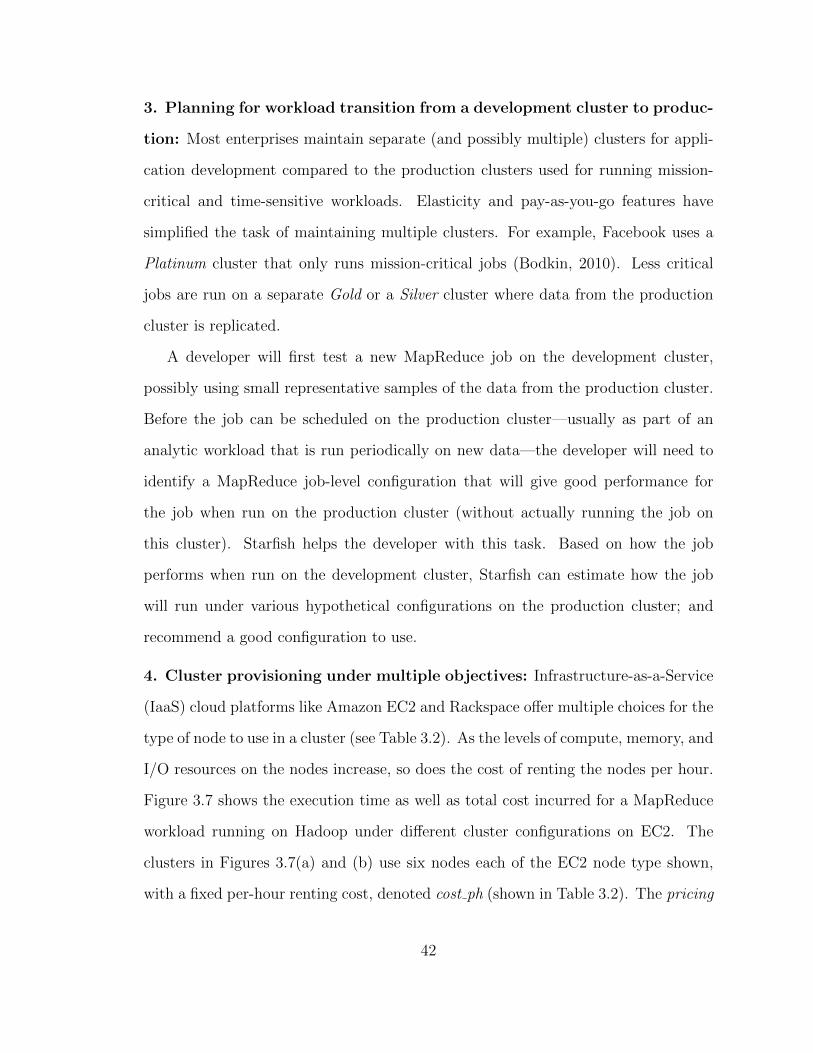
3.7 Performance Vs. pay-as-you-go costs for a workload that is run ondifferent EC2 cluster resource configurations. . . . . . . . . . . . . . . 43
3.8 Pay-as-you-go costs for a workload run on Hadoop clusters usingauction-based EC2 spot instances. . . . . . . . . . . . . . . . . . . . . 44
4.1 Map and reduce time breakdown for two Word Co-occurrence jobs runwith different settings for io.sort.mb. . . . . . . . . . . . . . . . . . . 53
4.2 Total map execution time, Spill time, and Merge time for a represen-tative Word Co-occurrence map task as we vary the setting of io.sort.mb. 54
4.3 (a) Overhead to measure the (approximate) profile, and (b) corre-sponding speedup given by Starfish as the percentage of profiled tasksis varied for Word Co-occurrence and TeraSort MapReduce jobs. . . . 59
xii
5.1 Screenshot from the Starfish Visualizer showing the execution timelineof the map and reduce tasks of a MapReduce job running on a Hadoopcluster. . . . . . . . . . . . . . . . . . . . . . . . . . . . . . . . . . . . 71
5.2 Screenshot from the Starfish Visualizer showing a histogram of themap output data size per map task. . . . . . . . . . . . . . . . . . . . 72
5.3 Screenshot from the Starfish Visualizer showing a visual representationof the data flow among the Hadoop nodes during a MapReduce jobexecution. . . . . . . . . . . . . . . . . . . . . . . . . . . . . . . . . . 73
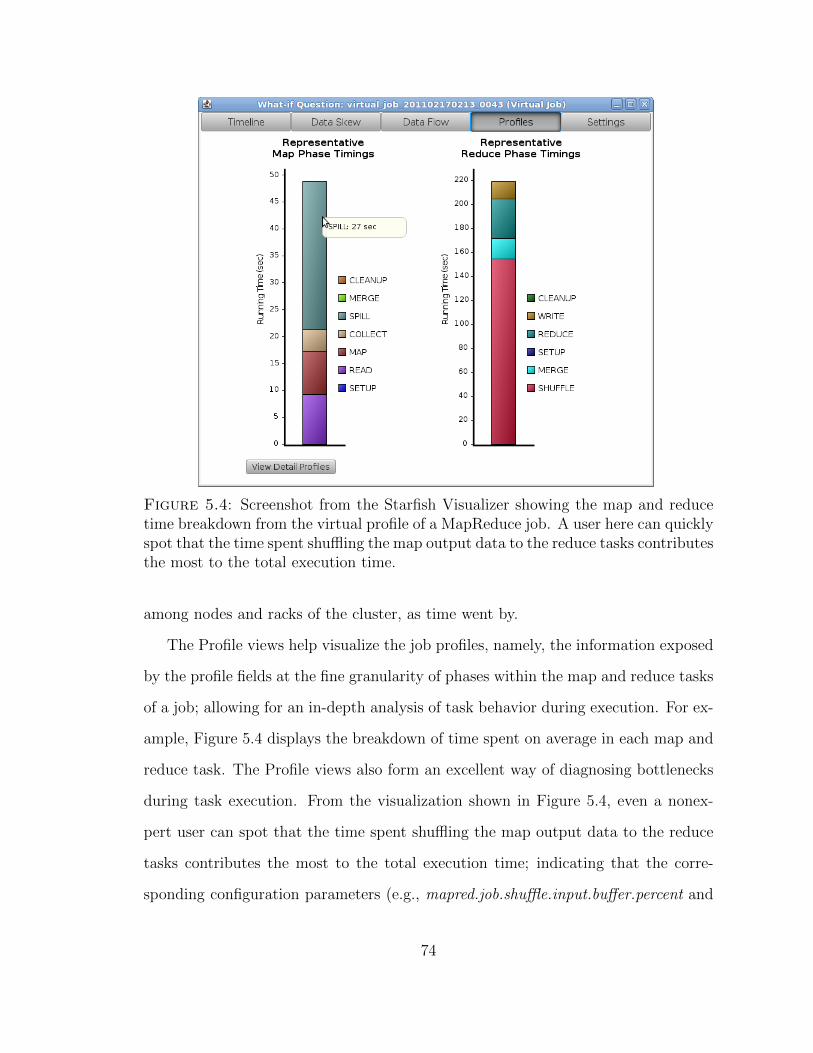
5.4 Screenshot from the Starfish Visualizer showing the map and reducetime breakdown from the virtual profile of a MapReduce job. . . . . . 74
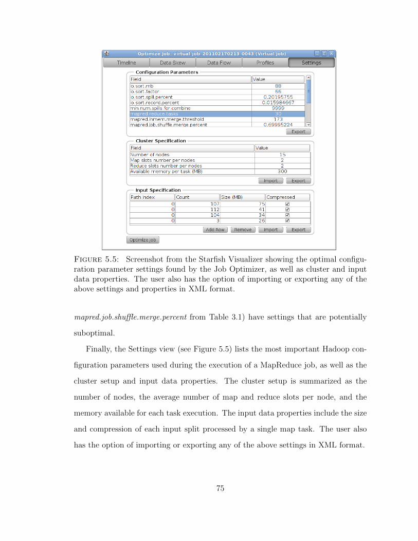
5.5 Screenshot from the Starfish Visualizer showing the optimal configura-tion parameter settings found by the Job Optimizer, as well as clusterand input data properties. . . . . . . . . . . . . . . . . . . . . . . . . 75
6.1 Overall process used by the What-if Engine to predict the performanceof a given MapReduce workflow. . . . . . . . . . . . . . . . . . . . . . 82
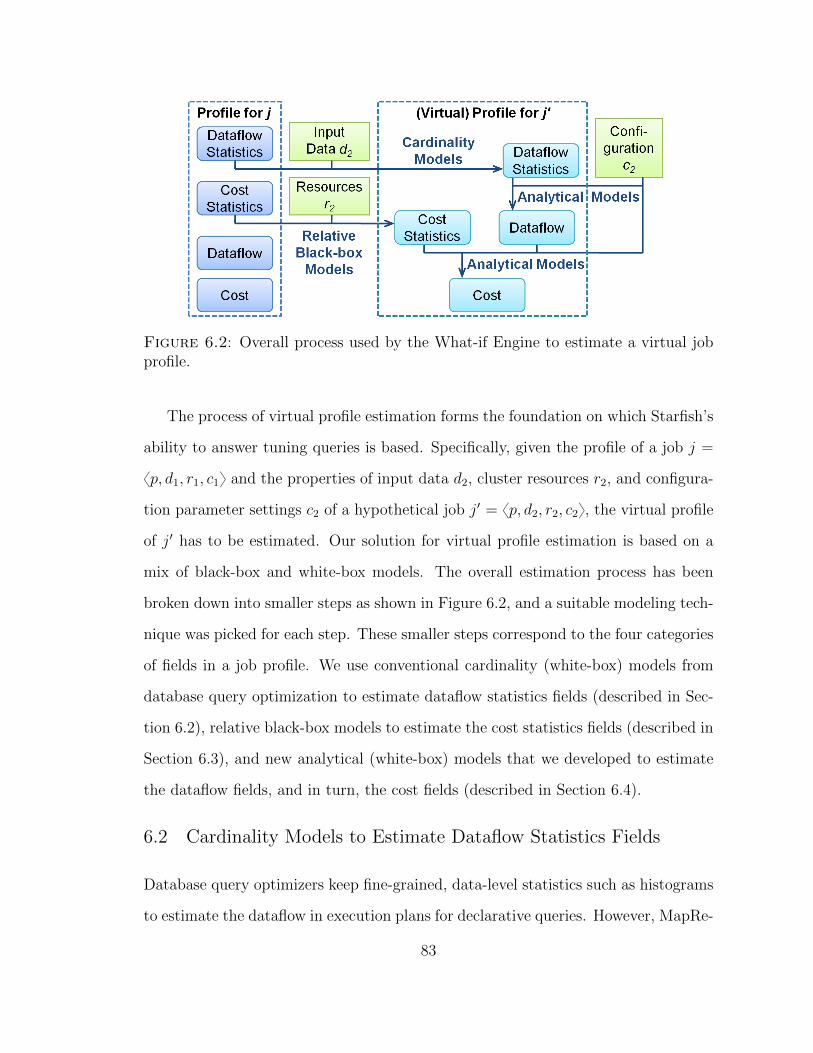
6.2 Overall process used by the What-if Engine to estimate a virtual jobprofile. . . . . . . . . . . . . . . . . . . . . . . . . . . . . . . . . . . . 83
6.3 Map and reduce time breakdown for Word Co-occurrence jobs from(A) an actual run and (B) as predicted by the What-if Engine. . . . . 113
6.4 Actual Vs. predicted running times for (a) Word Co-occurrence, (b)WordCount, and (c) TeraSort jobs running with different configurationparameter settings. . . . . . . . . . . . . . . . . . . . . . . . . . . . . 114
6.5 Actual and predicted running times for MapReduce jobs as the numberof nodes in the cluster is varied. . . . . . . . . . . . . . . . . . . . . . 115
6.6 Actual and predicted running times for MapReduce jobs when run onthe production cluster. . . . . . . . . . . . . . . . . . . . . . . . . . . 116
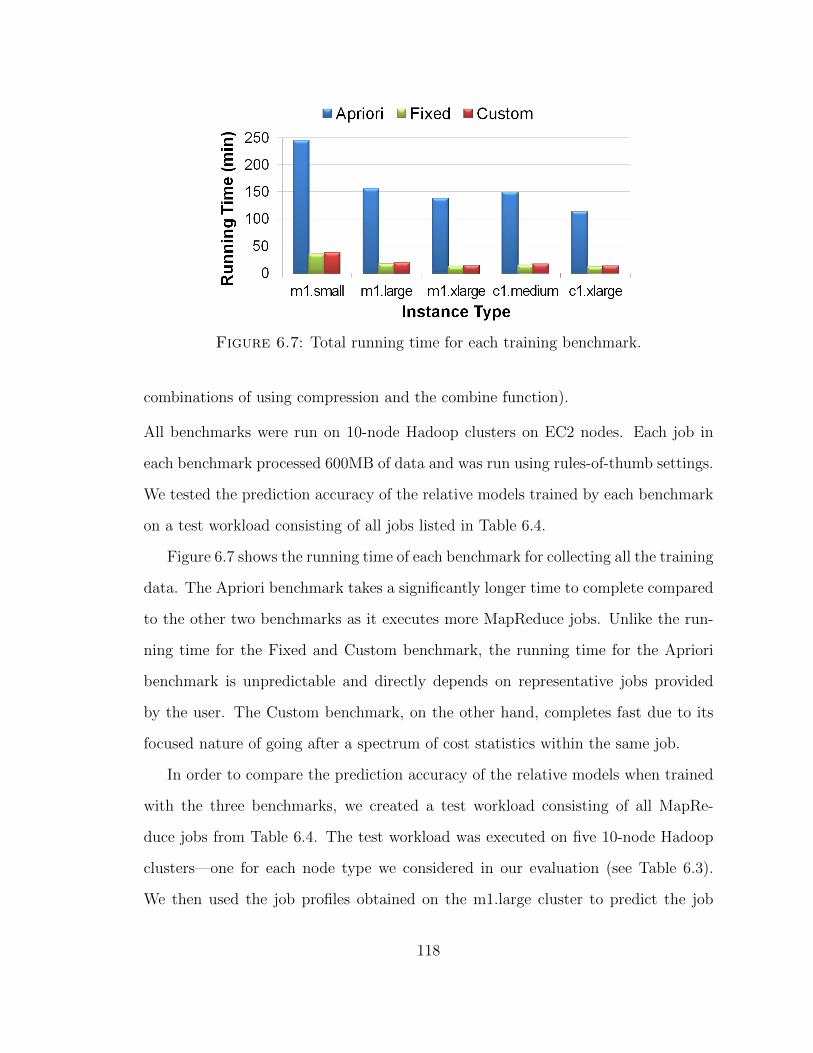
6.7 Total running time for each training benchmark. . . . . . . . . . . . . 118
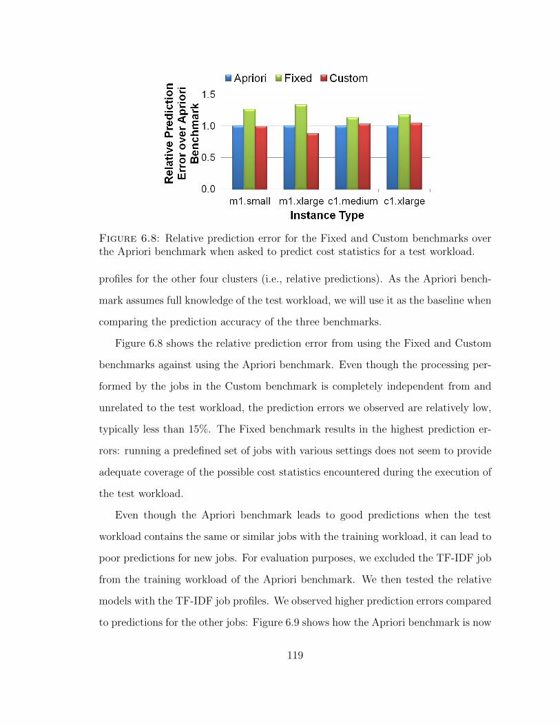
6.8 Relative prediction error for the Fixed and Custom benchmarks overthe Apriori benchmark when asked to predict cost statistics for a testworkload. . . . . . . . . . . . . . . . . . . . . . . . . . . . . . . . . . 119
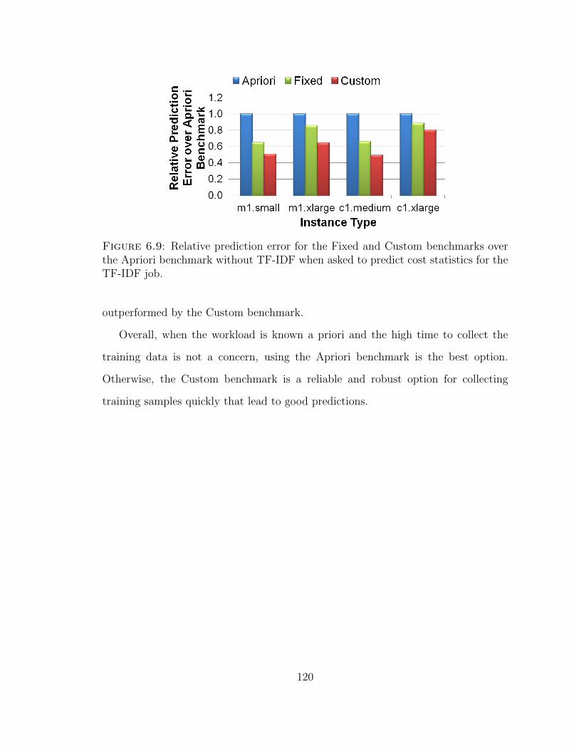
6.9 Relative prediction error for the Fixed and Custom benchmarks overthe Apriori benchmark without TF-IDF when asked to predict coststatistics for the TF-IDF job. . . . . . . . . . . . . . . . . . . . . . . 120
xiii
7.1 Overall process for optimizing a MapReduce job. . . . . . . . . . . . . 131
7.2 Map and reduce time breakdown for two Word Co-occurrence jobsrun with configuration settings suggested by Rules-of-Thumb and thecost-based Job Optimizer. . . . . . . . . . . . . . . . . . . . . . . . . 136
7.3 Running times for MapReduce jobs running with Hadoop’s Default,Rules-of-Thumb, and CBO-suggested settings. . . . . . . . . . . . . . 138
7.4 Optimization time for the six Cost-based Optimizers for various MapRe-duce jobs. . . . . . . . . . . . . . . . . . . . . . . . . . . . . . . . . . 139
7.5 Number of what-if calls made (unique configuration settings consid-ered) by the six Cost-based Optimizers for various MapReduce jobs. . 139
7.6 The job execution times for TeraSort when run with (a) Rules-of-Thumb settings, (b) CBO-suggested settings using a job profile ob-tained from running the job on the corresponding data size, and (c)CBO-suggested settings using a job profile obtained from running thejob on 5GB of data. . . . . . . . . . . . . . . . . . . . . . . . . . . . . 140
7.7 The job execution times for MapReduce programs when run with (a)Rules-of-Thumb settings, (b) CBO-suggested settings using a job pro-file obtained from running the job on the production cluster, and (c)CBO-suggested settings using a job profile obtained from running thejob on the development cluster. . . . . . . . . . . . . . . . . . . . . . 141
7.8 Percentage overhead of profiling on the execution time of MapReducejobs as the percentage of profiled tasks in a job is varied. . . . . . . . 142
7.9 Speedup over the job run with Rules-of-Thumb settings as the per-centage of profiled tasks used to generate the job profile is varied. . . 143
7.10 MapReduce workflows for (a) Query H4 from the Hive PerformanceBenchmark; (b) Queries P1 and P7 from the PigMix Benchmark runas one workflow; (c) Our custom example. . . . . . . . . . . . . . . . 144
7.11 Execution times for jobs in a workflow when run with settings sug-gested by (a) popular Rules of Thumb; (b) a Job-level Workflow Op-timizer; (c) an Interaction-aware Workflow Optimizer. . . . . . . . . . 146
7.12 Execution timeline for jobs in a workflow when run with settings sug-gested by (a) popular Rules of Thumb; (b) an Interaction-aware Work-flow Optimizer. . . . . . . . . . . . . . . . . . . . . . . . . . . . . . . 148
xiv
7.13 The optimization units (denoted with dotted boxes) for our exampleMapReduce workflow for the three Workflow Optimizers. . . . . . . . 153
7.14 Speedup achieved over the Rules-of-Thumb settings for workflows run-ning on the Amazon cluster from (a) the TPC-H Benchmark, (b) thePigMix Benchmark, and (c) the Hive Performance Benchmark. . . . . 162
7.15 Speedup achieved over the Rules-of-Thumb settings for workflows run-ning on the Yahoo! cluster from (a) the TPC-H Benchmark, (b) thePigMix Benchmark, and (c) the Hive Performance Benchmark. . . . . 163
7.16 Optimization overhead for all MapReduce workflows. . . . . . . . . . 164
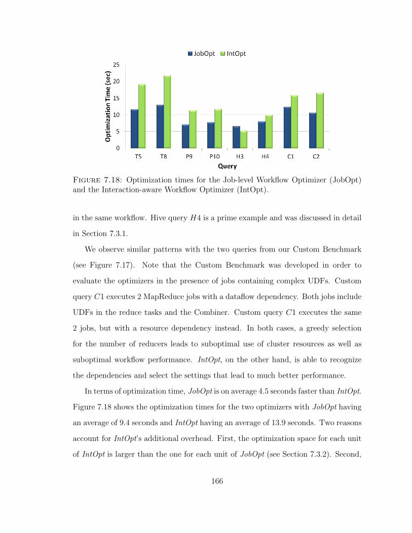
7.17 Running times of queries with settings based on Rules-of-Thumb, theJob-level Workflow Optimizer, and the Interaction-aware WorkflowOptimizer. . . . . . . . . . . . . . . . . . . . . . . . . . . . . . . . . . 165
7.18 Optimization times for the Job-level Workflow Optimizer and theInteraction-aware Workflow Optimizer. . . . . . . . . . . . . . . . . . 166
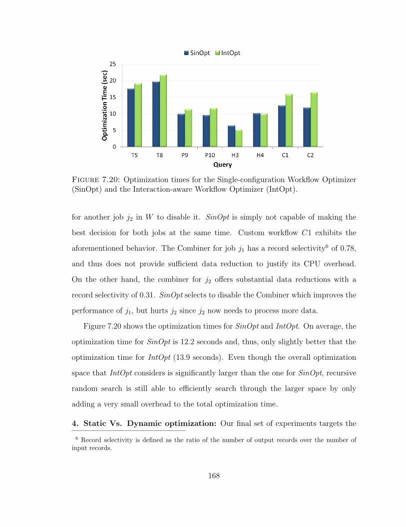
7.19 Running times of queries with settings based on Rules-of-Thumb, theSingle-configuration Workflow Optimizer, and the Interaction-awareWorkflow Optimizer. . . . . . . . . . . . . . . . . . . . . . . . . . . . 167
7.20 Optimization times for the Single-configuration Workflow Optimizerand the Interaction-aware Workflow Optimizer. . . . . . . . . . . . . 168
7.21 Running times of queries with settings based on Rules-of-Thumb, andthe Static and Dynamic Interaction-aware Workflow Optimizers. . . . 169
7.22 Running times of queries with settings based on Rules-of-Thumb, andthe Static and Dynamic Interaction-aware Workflow Optimizers, aswe vary the actual filter ratio of job j1. . . . . . . . . . . . . . . . . . 170
7.23 Running time and monetary cost of the workload when run with (a)Rules-of-Thumb settings and (b) Starfish-suggested settings, whilevarying the number of nodes and node types in the clusters. . . . . . 173
8.1 Neighborhoods and physical plans for our example star-join query. . . 179
8.2 Neighborhood and Cardinality Tables for our example star-join query. 183
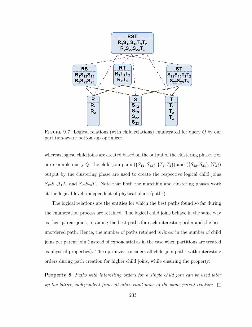
We have fully developed this approach for different tuning scenarios for both Dataflow
and Database systems. In particular, Starfish employs the profile-predict-optimize
approach for automatically tuning a MapReduce workload and cluster resources,
after observing the run-time behavior of the workload from a single execution. A
similar approach can be developed for Database systems, especially since several
mechanisms are already available (see Section 2.1). Instead, we employ the profile-
predict-optimize approach for the tuning scenario where the user or DBA is willing
to invest some resources upfront for tuning important, repeatedly-run SQL queries.
The Xplus optimizer profiles the execution of some query (sub)plans proactively,
optimizes the plan based on the collected monitoring data, and iterates, until it finds
the optimal query execution plan. We elaborate on these contributions below.
2.2.1 Tuning MapReduce Workloads with Starfish
Starfish is a MADDER and self-tuning system for analytics on Big Data (Herodotou
et al., 2011d). An important design decision we made was to build Starfish on
the Hadoop stack as shown in Figure 2.1. Hadoop, as observed in Chapter 1, has
useful primitives to help meet the new requirements of Big Data analytics (Hadoop,
2012). In addition, Hadoop’s adoption by academic, government, and industrial
organizations is growing at a fast pace (Gantz and Reinsel, 2011).
A number of ongoing projects aim to improve Hadoop’s peak performance, es-
pecially to match the query performance of parallel Database systems (Abouzeid
et al., 2009; Dittrich et al., 2010; Jiang et al., 2010). Starfish has a different goal.
The peak performance that a manually-tuned system can achieve is not our primary
concern, especially if this performance is for one of the many phases in a complete
20
Figure 2.1: Starfish in the Hadoop ecosystem.
data lifecycle that includes data loading, processing ad-hoc queries, running work-
flows repeatedly on newly arrived data, and data archival. Starfish’s goal is to enable
Hadoop users and applications to get good performance automatically throughout
the data lifecycle in analytics; without any need on their part to understand and
manipulate the many tuning knobs available.
The workload that a Hadoop deployment runs can be considered at different
levels. At the lowest level, Hadoop runs MapReduce jobs. A job can be generated
directly from a program written in a programming language like Java or Python;
or generated from a query in a higher-level language like HiveQL or Pig Latin; or
submitted as part of a MapReduce job workflow (i.e., a directed acyclic graph of
MapReduce jobs) by systems like Azkaban, Cascading, and Oozie (Azkaban, 2011;
Cascading, 2011; Oozie, 2010). The execution plan generated for a HiveQL or Pig
Latin query is usually a workflow of MapReduce jobs (Thusoo et al., 2009; Olston
et al., 2008b). Workflows may be ad-hoc, time-driven (e.g., run every hour), or data-
driven. Yahoo! uses data-driven workflows to generate a reconfigured preference
21
model and an updated home-page for any user within seven minutes of a home-page
click by the user.
Hadoop itself is typically run on a large cluster built of commodity hardware.
Clusters can now be easily provisioned by several cloud platforms like Amazon,
Rackspace, and Skytap. Elastic MapReduce, for example, is a hosted service on
the Amazon cloud platform where a user can instantly provision a Hadoop clus-
ter running on any number of Elastic Compute Cloud (EC2) nodes (Amazon EMR,
2012). The cluster can be used to run data-intensive MapReduce jobs, and then
terminated after use. The user has to pay (only) for the nodes provisioned to the
cluster for the duration of use.
Suppose a user wants to execute a given MapReduce workload on a Hadoop
cluster provisioned by the Amazon cloud platform. The user could have multiple
preferences and constraints for the workload. For example, the goal may be to mini-
mize the monetary cost incurred to run the workload, subject to a maximum tolerable
workload execution time of two hours. In order to satisfy these requirements, the
user must make a wide range of decisions. First, the user must decide the cluster
size and the type of resources to use in the cluster from the several choices offered by
the Amazon cloud platform. Next, the user must specify a large number of cluster-
wide Hadoop configuration parameters like the maximum number of map and reduce
tasks to execute per node and the maximum available memory per task execution.
To complicate the space of decisions even further, the user has to also specify what
values to use for a number of job-level Hadoop configuration parameters like the
number of reduce tasks and whether to compress job outputs. Chapter 3 includes
a primer on MapReduce execution and tuning, as well as multiple tuning scenarios
that arise routinely in practice.
As the above scenario illustrates, users are now faced with complex workload
tuning problems that involve determining the cluster resources as well as configuration
22
Figure 2.2: Components in the Starfish architecture.
settings to meet desired requirements on execution time and cost for a given analytic
workload. Starfish is a novel system to which users can express their tuning problems
as queries in a declarative fashion. Starfish can provide reliable answers to these
queries using an automated technique, and provide nonexpert users with a good
combination of cluster resource and configuration settings to meet their needs. The
automated technique is based on a careful mix of profiling, estimation using black-box
and white-box models, and simulation.
The Starfish architecture, shown in Figure 2.2, is motivated from the profile-
predict-optimize approach. Starfish includes a Profiler to collect detailed statistical
information from unmodified MapReduce programs, and a What-if Engine for fine-
grained cost estimation. The capabilities of the What-if Engine are utilized by a
number of Cost-based Optimizers that are responsible for enumerating and search-
ing efficiently through various spaces of tuning choices, in order to find the best
choices that meet the user requirements. Finally, the Tuning Query Interface and
the Visualizer provide the interfaces by which users interact with the Starfish system.
23
Profiler: The Profiler instruments unmodified MapReduce programs dynamically
to generate concise statistical summaries of MapReduce job execution, called job
profiles. A job profile consists of dataflow and cost estimates for a MapReduce job
j: dataflow estimates represent information regarding the number of bytes and key-
value pairs processed during j’s execution, while cost estimates represent resource
usage and execution time.
The Profiler makes two important contributions. First, job profiles capture in-
formation at the fine granularity of phases within the map and reduce tasks of a
MapReduce job execution. This feature is crucial to the accuracy of decisions made
by the What-if Engine and the Cost-based Optimizers. Second, the Profiler uses dy-
namic instrumentation to collect run-time monitoring information from unmodified
MapReduce programs. The dynamic nature means that monitoring can be turned
on or off on demand; an appealing property in production deployments. By support-
ing unmodified MapReduce programs, we free users from any additional burden on
their part to collect monitoring information. Dynamic profiling and the Profiler are
discussed in detail in Chapter 4.
What-if Engine: The What-if Engine1 is the heart of our approach to cost-based
optimization and automated tuning. Apart from being invoked by the Cost-based
Optimizers during program optimization, the What-if Engine can be invoked in stan-
dalone mode by users or applications to answer questions regarding the impact of
configuration parameter settings, as well as data and cluster resource properties, on
MapReduce workload performance.
The What-if Engine’s novelty and accuracy come from how it uses a mix of sim-
ulation and model-based estimation at the phase level of MapReduce job execution.
1 The term “what-if” also appears in the context of automated physical design in Databasesystems (Chaudhuri and Narasayya, 2007), where the scope of the what-if questions consists ofphysical design choices (e.g., indexes, materialized views) rather than tuning choices.
24
The What-if Engine uses a four-step process. First, a virtual job profile is estimated
for each hypothetical job j1 specified by the what-if question. The virtual profile
is then used to simulate the execution of j1 on the (perhaps hypothetical) cluster,
as well as to estimate the data properties for the derived dataset(s) produced by
j1. Finally, the answer to the what-if question is computed based on the estimated
execution of j1. All performance models and components of the What-if Engine are
presented in Chapter 6.
Cost-based Optimizers: For a given MapReduce workflow, input data, and clus-
ter resources, an optimizer’s role is to enumerate and search through the high-
dimensional space of tuning choices efficiently, making appropriate calls to the What-
if Engine, in order to find the (near) optimal choice. The space of possible tuning
choices consists of (i) the subspace of cluster resource settings—which includes the
number of nodes in the cluster as well as the type of each node in the cluster—and (ii)
the high-dimensional subspace of configuration parameter settings—which includes
parameters such as the degree of parallelism, memory settings, use of map-side and
reduce-side compression, and many others.
The search space is enumerated and traversed using three Optimizers (see Figure
2.2). The Job Optimizer is responsible for finding good configuration settings for
individual MapReduce jobs (Herodotou and Babu, 2011). The jobs in a workflow
exhibit dataflow dependencies because of producer-consumer relationships as well
as cluster resource dependencies because of concurrent scheduling. The Workflow
Optimizer carefully optimizes the workflow execution within and across jobs, while
accounting for these dependencies (Herodotou et al., 2012). Finally, the Cluster
Resource Optimizer is responsible for the subspace of cluster resource settings and
can help with making cluster provisioning decisions (Herodotou et al., 2011b).
The number of calls to the What-if Engine has to be minimized for efficiency,
25
without sacrificing the ability to find good tuning settings. Towards this end, all
optimizers divide the full space of tuning choices into lower-dimensional subspaces
such that the globally-optimal choices in the high-dimensional space can be generated
by composing the optimal choices found for the subspaces. The overall cost-based
optimization approach is discussed in Chapter 7.
Tuning Query Interface and Visualizer: A general tuning problem involves
determining the cluster resources and MapReduce job-level configuration settings
to meet desired performance requirements on execution time and cost for a given
analytic workload. Starfish provides a declarative interface to express a range of
tuning problems as queries in a declarative fashion. A query expressed using this
interface will specify (i) the MapReduce workload, (ii) the search space for cluster
resources, (iii) the search space for job configurations, and (iv) the performance
requirements in terms of time and monetary cost. Applications and users can also
interact with this interface using a programmatic API, or using a graphical interface
that forms part of the Starfish system’s Visualizer (Herodotou et al., 2011a). The
Tuning Query Interface and the Starfish Visualizer are presented in Chapter 5.
2.2.2 Tuning SQL Queries with Xplus
The profile-predict-optimize approach used currently in Starfish is just one cycle
of a more general self-tuning approach that learns repeatedly over time and re-
optimizes as needed. In this spirit, we propose experiment-driven tuning of im-
portant, repeatedly-run SQL queries in Database systems. The need to improve a
suboptimal execution plan picked by the query optimizer for a repeatedly-run SQL
query (e.g., by a business intelligence or report generation application) arises rou-
tinely in MADDER settings. Unknown or stale statistics, complex expressions, and
changing conditions can cause the optimizer to make mistakes. In Chapter 8, we
present a novel SQL-tuning-aware query optimizer, called Xplus (Herodotou and
26
Babu, 2010), that is capable of executing plans proactively, collecting monitoring
data from the runs, and iterating, in search for a better execution plan.
Finally, despite the recent advances in query optimization techniques, Database
and Dataflow systems still struggle with the decreased control over data storage and
data structure mandated by the MADDER principles. Careful data layouts and
partitioning strategies are powerful mechanisms for improving query performance
and system manageability in these systems. SQL extensions and MapReduce frame-
works now enable applications and user queries to specify how their results should
be partitioned for further use, decreasing the control that database administrators
had previously over partitioning. However, query optimization techniques have not
kept pace with the rapid advances in usage and user control of table partitioning.
We address this gap by developing new techniques to generate efficient plans for SQL
queries involving multiway joins over partitioned tables (Herodotou et al., 2011c).
These techniques are presented in Chapter 9.
27
3
Primer on Tuning MapReduce Workloads
MapReduce is a relatively young framework—both a programming model and an
associated run-time system—for large-scale data processing (Dean and Ghemawat,
2008). Hadoop is the most popular open-source implementation of a MapReduce
framework that follows the design laid out in the original paper (Dean and Ghe-
mawat, 2004). A number of companies use Hadoop in production deployments for
applications such as Web indexing, data mining, report generation, log file analy-
sis, machine learning, financial analysis, scientific simulation, and bioinformatics re-
search. Infrastructure-as-a-Service cloud platforms like Amazon and Rackspace have
made it easier than ever to run Hadoop workloads by allowing users to instantly
provision clusters and pay only for the time and resources used. A combination
of features contributes to Hadoop’s increasing popularity, including fault tolerance,
data-local scheduling, ability to operate in a heterogeneous environment, handling
of straggler tasks1, as well as a modular and customizable architecture.
In this chapter, we provide an overview of the MapReduce programming model
and describe how MapReduce programs execute on a Hadoop cluster. The behavior
1 A straggler is a task that performs poorly typically due to faulty hardware or misconfiguration.
28
Figure 3.1: Execution of a MapReduce job.
of MapReduce job execution is affected by a large number of configuration parameter
settings. We will provide empirical evidence of the significant impact that parameter
settings can have on the performance of a MapReduce job. Finally, we will list
various optimization and tuning scenarios that arise routinely in practice.
3.1 MapReduce Job Execution
The MapReduce programming model consists of two functions: mappk1, v1q and
reducepk2, listpv2qq. Users can implement their own processing logic by specifying
a customized mappq and reducepq function written in a general-purpose language like
Java or Python. The mappk1, v1q function is invoked for every key-value pair xk1, v1y
in the input data to output zero or more key-value pairs of the form xk2, v2y (see
Figure 3.1). The reducepk2, listpv2qq function is invoked for every unique key k2 and
corresponding values listpv2q in the map output. reducepk2, listpv2qq outputs zero or
more key-value pairs of the form xk3, v3y. The MapReduce programming model also
allows other functions such as (i) partitionpk2q, for controlling how the map output
key-value pairs are partitioned among the reduce tasks, and (ii) combinepk2, listpv2qq,
for performing partial aggregation on the map side. The keys k1, k2, and k3 as well
29
Figure 3.2: Execution of a map taskshowing the map-side phases.
Figure 3.3: Execution of a reduce taskshowing the reduce-side phases.
as the values v1, v2, and v3 can be of different and arbitrary types.
A Hadoop MapReduce cluster employs a master-slave architecture where one mas-
ter node (called JobTracker) manages a number of slave nodes (called TaskTrackers).
Figure 3.1 shows how a MapReduce job is executed on the cluster. Hadoop launches
a MapReduce job by first splitting (logically) the input dataset into data splits. Each
data split is then scheduled to one TaskTracker node and is processed by a map task.
A Task Scheduler is responsible for scheduling the execution of map tasks while tak-
ing data locality into account. Each TaskTracker has a predefined number of task
execution slots for running map (reduce) tasks. If the job will execute more map
(reduce) tasks than there are slots, then the map (reduce) tasks will run in multiple
waves. When map tasks complete, the run-time system groups all intermediate key-
value pairs using an external sort-merge algorithm. The intermediate data is then
shuffled (i.e., transferred) to the TaskTrackers scheduled to run the reduce tasks.
Finally, the reduce tasks will process the intermediate data to produce the results of
the job.
The MapReduce job execution can be decomposed further into phases within map
and reduce tasks. As illustrated in Figure 3.2, map task execution consists of the
following phases: Read (reading map inputs), Map (map function processing), Collect
30
(partitioning and buffering map outputs before spilling), Spill (sorting, combining,
compressing, and writing map outputs to local disk), and Merge (merging sorted spill
files). As illustrated in Figure 3.3, reduce task execution consists of the following
phases: Shuffle (transferring map outputs to reduce tasks, with decompression if
needed), Merge (merging sorted map outputs), Reduce (reduce function processing),
and Write (writing reduce outputs to the distributed file-system). Additionally, both
map and reduce tasks have Setup and Cleanup phases.
A MapReduce workload consists of MapReduce jobs of the form j = xp, d, r, cy.
Here, p represents the MapReduce program that is run as part of j to process input
data d on cluster resources r using configuration parameter settings c.
Program: A given MapReduce program p may be expressed in one among a variety
of programming languages like Java, C++, Python, or Ruby; and then connected to
form a workflow using a workflow scheduler like Oozie (Oozie, 2010). Alternatively,
the MapReduce jobs can be generated automatically using compilers for higher-level
languages like Pig Latin (Olston et al., 2008b), HiveQL (Thusoo et al., 2009), and
Cascading (Cascading, 2011).
Data: The properties of the input data d processed by a MapReduce job j include
d’s size, the block layout of files that comprise d in the distributed file-system, and
whether d is stored compressed or not. Since the MapReduce methodology is to
interpret data (lazily) at processing time, and not (eagerly) at loading time, other
properties such as the schema and data-level distributions of d are unavailable by
default.
Cluster resources: The properties of the cluster resources r that are available for a
job execution include the number of nodes in the cluster, the machine specifications
(or the node type when the cluster is provisioned by a cloud platform like Amazon
EC2), the cluster’s network topology, the number of map and reduce task execution
31
slots per node, and the maximum memory available per task execution slot.
Configuration parameter settings: A number of choices have to be made in
order to fully specify how the job should execute. These choices, represented by c in
xp, d, r, cy, come from a large and high-dimensional space of configuration parameter
settings that includes (but is not limited to):
1. The number of map tasks in job j. Each task processes one partition (split)
of the input data d. These tasks may run in multiple waves depending on the
total number of map task execution slots in r.
2. The number of reduce tasks in j (which may also run in waves).
3. The amount of memory to allocate to each map (reduce) task to buffer its
output (input) data.
4. The settings for the multiphase external sorting used by most MapReduce
frameworks to group map-output values by key.
5. Whether the output data from the map (reduce) tasks should be compressed
before being written to disk (and if so, then how).
6. Whether the program-specified combine function should be used to preaggre-
gate map outputs before their transfer to reduce tasks.
Hadoop has more than 190 configuration parameters out of which Starfish currently
considers 14 parameters whose settings can have significant impact on job perfor-
mance (Herodotou et al., 2011d). These parameters are listed on Table 3.1. If the
user does not specify parameter settings during job submission, then default values—
shipped with the system or specified by the system administrator—are used. Good
settings for these parameters depend on job, data, and cluster characteristics. While
32
Table 3.1: A subset of important job configuration parameters in Hadoop.
Parameter Name Brief Description and Use DefaultValue
io.sort.mb Size (in MB) of map-side buffer for storing and sort-ing key-value pairs produced by the map function
100
io.sort.record.percent Fraction of io.sort.mb dedicated to metadata stor-age for every key-value pair stored in the map-sidebuffer
0.05
io.sort.spill.percent Usage threshold of map-side memory buffer to trig-ger a sort and spill of the stored key-value pairs
0.8
io.sort.factor Number of sorted streams to merge at once duringthe multiphase external sorting
10
mapreduce.combine.class
The (optional) combine function to preaggregatemap outputs before transferring to the reduce tasks
null
min.num.spills.for.com-bine
Minimum number of spill files at which to use thecombine function during the merging of map outputdata
3
mapred.compress.map.output
Boolean flag to turn on the compression of map out-put data
false
mapred.reduce.slowstart.completed.maps
Proportion of map tasks that need to be completedbefore any reduce tasks are scheduled
0.05
mapred.reduce.tasks Number of reduce tasks 1
mapred.job.shuffle.input.buffer.percent
% of reduce task’s heap memory used to buffer out-put data copied from map tasks during the shuffle
0.7
mapred.job.shuffle.merge.percent
Usage threshold of reduce-side memory buffer totrigger reduce-side merging during the shuffle
0.66
mapred.inmem.merge.threshold
Threshold on the number of copied map outputs totrigger reduce-side merging during the shuffle
1000
mapred.job.reduce.input.buffer.percent
% of reduce task’s heap memory used to buffer mapoutput data while applying the reduce function
0
mapred.output.compress Boolean flag to turn on the compression of the job’soutput
false
only a fraction of the parameters can have significant performance impact, browsing
through the Hadoop, Hive, and Pig mailing lists reveals that users often run into
performance problems caused by lack of knowledge of these parameters.
MapReduce workflow: A MapReduce workflow W is a directed acyclic graph
(DAG) GW that represents a set of MapReduce jobs and their dataflow dependencies.
Each vertex in GW is either a MapReduce job j or a dataset d. An edge in GW can
only exist between a job (vertex) j and a dataset (vertex) d. A directed edge (d
Ñ j) denotes d as an input dataset of job j; and a directed edge (j Ñ d) denotes
33
Figure 3.4: An example MapReduce workflow with four MapReduce jobs (j1-j4),two base datasets (b1, b2), and four derived datasets (d1-d4).
d as an output dataset of j. The datasets processed by a given workflow W are
categorized into base and derived datasets. Base datasets (basepW q) represent the
existing data consumed by W , whereas derived datasets (derivedpW q) represent the
data generated by the MapReduce programs in W .
Figure 3.4 shows an example workflow with four MapReduce jobs (j1-j4), two
base datasets (b1, b2), and four derived datasets (d1-d4). The distinction between
base and derived data will become important in Chapter 6 where we discuss how we
can answer hypothetical questions regarding the execution of a MapReduce workflow.
Abstractions in Starfish: In order to support the wide and growing variety of
MapReduce programs and the programming languages in which they are expressed,
Starfish represents the execution of a MapReduce job j using a job profile. This profile
is a concise summary of the dataflow and cost information for job j’s execution
Similar to a job profile, a workflow profile is used to represent the execution of a
MapReduce workflow W on the cluster. Chapter 4 discusses the content of the job
and workflow profiles, as well as how these profiles are generated.
34
3.2 Impact of Configuration Parameter Settings
The Hadoop configuration parameters control various aspects of job behavior during
execution, such as memory allocation and usage, concurrency, I/O optimization, and
network bandwidth usage. To illustrate the impact of job configuration parameters
in Hadoop, we study the effects of several parameter settings on the performance
of two MapReduce programs. The experimental setup used is a single-rack Hadoop
cluster running on 16 nodes, with 1 master and 15 slave nodes, provisioned from
Amazon Elastic Compute Cloud (EC2). Each node has 1.7 GB of memory, 5 EC2
compute units, 350 GB of storage, and is set to run at most 3 map tasks and 2 reduce
tasks concurrently. Thus, the cluster can run at most 45 map tasks in a concurrent
map wave, and at most 30 reduce tasks in a concurrent reduce wave. Table 3.1 lists
the subset of job configuration parameters that we considered in our experiments.
The MapReduce jobs we consider are WordCount and TeraSort2; two simple,
yet representative, text processing jobs with well-understood characteristics. Word-
Count processes 30GB of data generated using Hadoop’s RandomTextWriter, while
TeraSort processes 50GB of data generated using Hadoop’s TeraGen. Figures 3.5
and 3.6 show the response surfaces that were generated by measuring the execution
time of the WordCount and TeraSort jobs respectively. The three parameters varied
in these figures are io.sort.mb, io.sort.record.percent, and mapred.reduce.tasks, while
all other job configuration parameters are kept constant.
The effects of the parameter settings on the performance of a MapReduce job
depend on job, data, and cluster characteristics:
Effect of job characteristics: Figures 3.5(a) and 3.6(a) show how the setting of
the mapred.reduce.tasks parameter (i.e., the number of reducers) affect WordCount
and TeraSort in different ways. Increasing the number of reducers has no impact on
2 TeraSort was used on a Hadoop cluster at Yahoo! to win the TeraByte Sort Benchmark in 2008.
35
(a) mapred.reduce.tasks P r2, 50s andio.sort.record.percent P r0.05, 0.5s
(b) io.sort.record.percent P r0.05, 0.5s
and io.sort.mb P r50, 200s
Figure 3.5: Response surfaces of WordCount MapReduce jobs in Hadoop.
(a) mapred.reduce.tasks P r27, 400s andio.sort.record.percent P r0.05, 0.5s
(b) io.sort.record.percent P r0.05, 0.5s
and io.sort.mb P r50, 200s
Figure 3.6: Response surfaces of TeraSort MapReduce jobs in Hadoop.
performance for WordCount across all settings of io.sort.record.percent, whereas it
improves the performance for TeraSort significantly. The job execution of WordCount
is dominated by the execution of the map tasks. Computation in the map tasks
includes the parsing of the input files, as well as applying a combine function, whereas
the reduce tasks are simply summing the word counts.
On the other hand, the map and reduce functions in TeraSort process the same
36
amount of data overall and perform the same task of simply writing all input values
directly to output. Increasing the number of reduce tasks improves performance due
to: (i) the increase in effective concurrency by utilizing more of the reduce slots in the
cluster (recall that our cluster has 30 reducer slots across 15 worker nodes), and (ii)
the processing of less data by each reduce task, since the overall data size processed
is fixed (which in turn can reduce I/O in nonlinear ways).
Effect of data characteristics: Data characteristics—like number of unique key
values, key-value distributions, as well as input and intermediate record sizes—can
effect the running time of job executions of the same MapReduce program, running
with the same parameter settings. The surface area of Figure 3.6(a) contains a
“valley” when the value for io.sort.record.percent is set to 0.15. io.sort.record.percent
represents the fraction of the map’s heap size that is dedicated to metadata storage
for the map’s output. Each record produced by the mapper requires 16 bytes of
metadata in addition to its serialized size. Given any value for this parameter, the
average map output record size will determine whether a spill to disk is caused by
exhaustion of the serialization buffer or by exhaustion of the metadata buffer.
Based on the current data characteristics, setting io.sort.record.percent to 0.15
maximizes the use of both buffers, leading to good job performance (see Figure
3.6(a)). Suppose we were to run TeraSort with the same parameter settings on a
new data set, where the average input record size is half the current size. Then,
the metadata buffer would become full when only half the serialization buffer is full,
causing a larger number of spills than necessary; thereby increasing the execution
time of the map tasks and the job. In other words, the valley in the surface area of
Figure 3.6(a) would shift to a larger value for io.sort.record.percent compared to the
current surface area.
Effect of cluster characteristics: The number of nodes in a cluster, the number
37
of map and reduce slots per node, the memory available for each task execution, and
the network setup are the prime cluster characteristics that can affect the impact
of parameter settings in job performance. For example, the number of reduce slots
determines the effective concurrency of the reduce computations. When the total
number of reduce tasks T is lower than the number of slots S, all reduce tasks
will run concurrently. Changing the number of reducers while T ď S will have a
significant effect on job performance, assuming the reduce task’s execution time is
comparable to the map task’s execution time. When T ą S, the reducers will run in
waves. In Figure 3.6(a), we observe that as the number of reduce tasks increases, the
performance improves but the rate of improvement decreases because of the bound
on effective concurrency per wave, as well as task setup overheads.
Interaction among parameters: A fairly large subset of the configuration pa-
rameters in Hadoop display strong performance interactions with one or more other
parameters. An interaction exists between parameters p1 and p2 when the mag-
nitude of impact that varying p1 has on job performance depends on the specific
setting of p2. Stated otherwise, the performance impact of varying p1 is different
across different settings of p2. For example, Figure 3.5(b) shows that for low settings
of io.sort.record.percent, the job performance is not affected significantly by vary-
ing io.sort.mb. However, for high settings of io.sort.record.percent, the performance
changes drastically while varying io.sort.mb. Figure 3.6(b) shows stronger and more
complicated interactions between io.sort.record.percent and io.sort.mb. Across dif-
ferent values of io.sort.record.percent, even the pattern of change in performance is
different as io.sort.mb is varied.
38
3.3 MapReduce on the Cloud
Infrastructure-as-a-Service (IaaS) cloud platforms provide computation, software,
data access, and storage resources to a number of users, while the details of the
underlying infrastructure are completely transparent. This computing paradigm is
attracting increasing interest from both academic researchers and industry data prac-
titioners because it enables MapReduce users to scale their applications up and down
seamlessly in a pay-as-you-go manner. Elastic MapReduce, for example, is a hosted
service on the Amazon cloud platform where a user can instantly provision a Hadoop
cluster running on any number of Elastic Compute Cloud (EC2) nodes (Amazon
EMR, 2012). The cluster can be used to run data-intensive MapReduce jobs, and
then terminated after use. The user has to pay (only) for the nodes provisioned to
the cluster for the duration of use.
The new and remarkable aspect here is that a nonexpert MapReduce user can
provision a cluster of any size on the cloud within minutes to meet her data-processing
needs. This feature of the cloud gives tremendous power to the average user, while
placing a major burden on her shoulders. Previously, the same user would have
had to work with system administrators and management personnel to get a cluster
provisioned for her needs. Many days to months would have been needed to complete
the provisioning process. Furthermore, making changes to an already-provisioned
cluster was a hassle.
Cloud platforms make cluster provisioning almost instantaneous. The elastic and
pay-as-you-go nature of these platforms means that, depending on how best to meet
her needs, a user can allocate a 10-node cluster today, a 100-node cluster tomorrow,
and a 25-node cluster the day after. However, removing the system administrator
and the traditional capacity-planning process from the loop shifts the nontrivial
responsibility of determining a good cluster configuration to the nonexpert user.
39
Table 3.2: Five representative Amazon EC2 node types, along with resources andmonetary costs.
EC2 Node CPU Memory Storage I/O CostType (# EC2 Units) (GB) (GB) Performance (U.S. $ per hour)
m1.small 1 1.7 160 moderate 0.085m1.large 4 7.5 850 high 0.34m1.xlarge 8 15 1,690 high 0.68c1.medium 5 1.7 350 moderate 0.17c1.xlarge 20 7 1,690 high 0.68
As an illustrative example, consider provisioning a Hadoop cluster on Amazon
EC2 nodes to run a MapReduce workload on the cloud. Services like Elastic MapRe-
duce and Hadoop On Demand free the user from having to install and maintain the
Hadoop cluster. However, the burden of cluster provisioning is still on the user, who
is likely not an expert system administrator. In particular, the user has to specify
the number of EC2 nodes to use in the cluster, as well as the node type to use from
among 10+ EC2 node types. Table 3.2 shows the features and renting costs of some
representative EC2 node types. Notice that the CPU and I/O resources available on
these node types are quoted in abstract terms that an average user will have trouble
understanding. To complicate the space of choices even further, the user has to spec-
ify what values to use for a number of configuration parameters—e.g., the number of
reduce tasks or whether to compress map outputs—at the level of MapReduce job
execution on the cluster (Babu, 2010; Herodotou and Babu, 2011).
3.4 Use Cases for Tuning MapReduce Workloads
In this work, we refer to the general problem of determining the cluster resources and
MapReduce job-level configuration parameter settings to meet desired requirements
on execution time and cost for a given analytic workload as the tuning problem. Users
can express tuning problems as declarative queries to Starfish, for which Starfish will
provide reliable answers in an automated fashion. In order to illustrate how Starfish
40
benefits users and applications, we begin by discussing some common scenarios where
tuning problems arise.
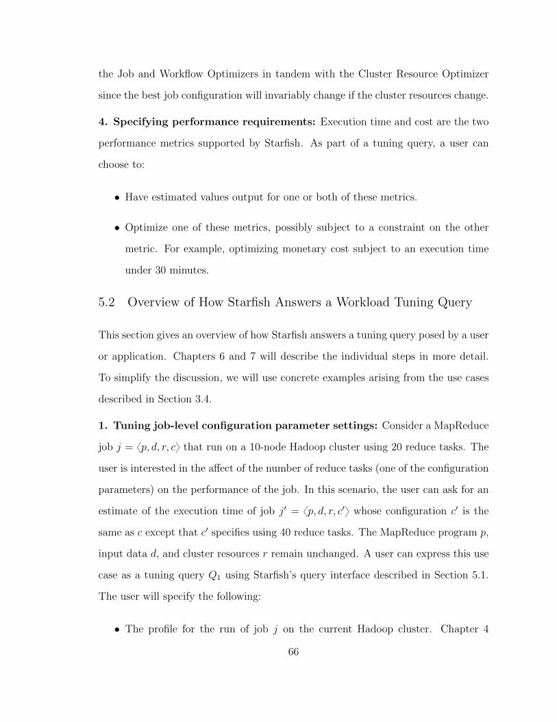
1. Tuning job-level configuration parameter settings: Even to run a single
job in a MapReduce framework, a number of configuration parameters have to be
set by users or system administrators. Users often run into performance problems
because they do not know how to set these parameters, or because they do not even
know these parameters exist. In other cases, the performance of a MapReduce job or
workflow simply does not meet the Service Level Objectives (SLOs) on response time
or workload completion time. Hence, the need for understanding the job behavior
as well as diagnosing bottlenecks during job execution for the parameter settings
used arises frequently. Even when users understand how a program behaved dur-
ing a specific run, they still cannot predict how the execution of the program will
be affected when parameter settings change, or which parameters should they use
to improve performance. Nonexpert users can now employ Starfish to (a) get a
deep understanding of a MapReduce program’s behavior during execution, (b) ask
hypothetical questions on how the program’s behavior will change when parame-
ter settings, cluster resources, or input data properties change, and (c) ultimately
optimize the program.
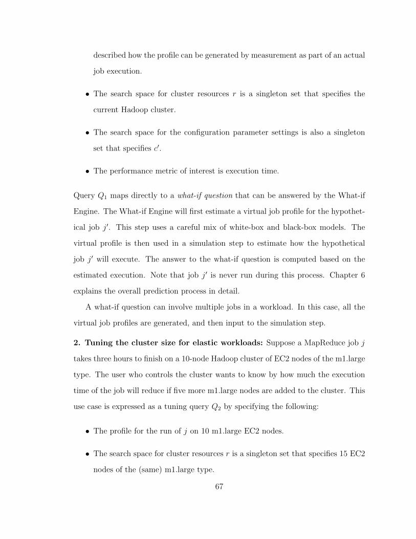
2. Tuning the cluster size for elastic workloads: Suppose a MapReduce job
takes three hours to finish on a 10-node Hadoop cluster of EC2 nodes of the m1.large
type. The application or the user who controls the cluster may want to know by
how much the execution time of the job will reduce if five more m1.large nodes are
added to the cluster. Alternatively, the user might want to know how many m1.large
nodes must be added to the cluster to reduce the running time down to two hours.
Such questions also arise routinely in practice, and can be answered automatically
by Starfish.
41
3. Planning for workload transition from a development cluster to produc-
tion: Most enterprises maintain separate (and possibly multiple) clusters for appli-
cation development compared to the production clusters used for running mission-
critical and time-sensitive workloads. Elasticity and pay-as-you-go features have
simplified the task of maintaining multiple clusters. For example, Facebook uses a
Platinum cluster that only runs mission-critical jobs (Bodkin, 2010). Less critical
jobs are run on a separate Gold or a Silver cluster where data from the production
cluster is replicated.
A developer will first test a new MapReduce job on the development cluster,
possibly using small representative samples of the data from the production cluster.
Before the job can be scheduled on the production cluster—usually as part of an
analytic workload that is run periodically on new data—the developer will need to
identify a MapReduce job-level configuration that will give good performance for
the job when run on the production cluster (without actually running the job on
this cluster). Starfish helps the developer with this task. Based on how the job
performs when run on the development cluster, Starfish can estimate how the job
will run under various hypothetical configurations on the production cluster; and
recommend a good configuration to use.
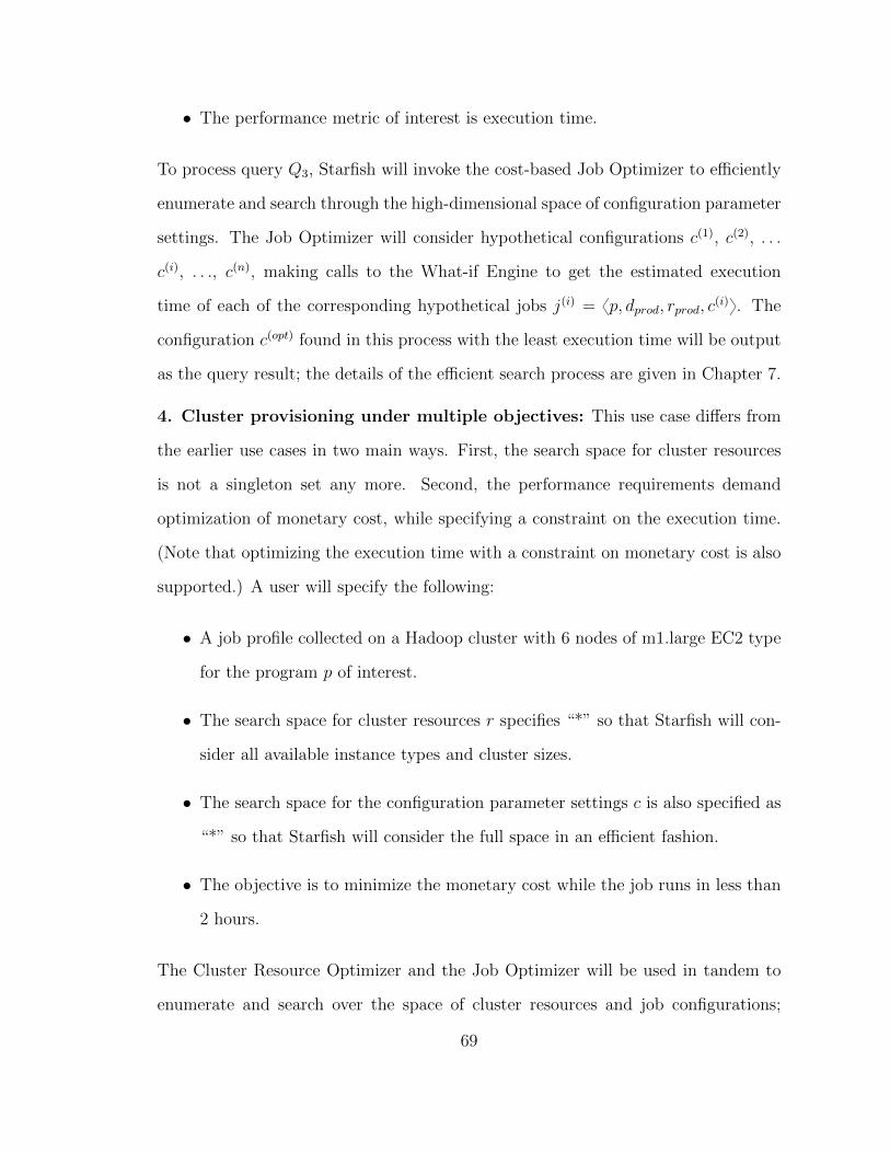
4. Cluster provisioning under multiple objectives: Infrastructure-as-a-Service
(IaaS) cloud platforms like Amazon EC2 and Rackspace offer multiple choices for the
type of node to use in a cluster (see Table 3.2). As the levels of compute, memory, and
I/O resources on the nodes increase, so does the cost of renting the nodes per hour.
Figure 3.7 shows the execution time as well as total cost incurred for a MapReduce
workload running on Hadoop under different cluster configurations on EC2. The
clusters in Figures 3.7(a) and (b) use six nodes each of the EC2 node type shown,
with a fixed per-hour renting cost, denoted cost ph (shown in Table 3.2). The pricing
42
Figure 3.7: Performance Vs. pay-as-you-go costs for a workload that is run ondifferent EC2 cluster resource configurations.
model used to compute the corresponding total cost of each workload execution is:
total cost “ cost phˆ num nodesˆ exec time (3.1)
Here, num nodes is the number of nodes in the cluster and exec time is the execu-
tion time of the workload rounded up to the nearest hour as done on most cloud
platforms. The user could have multiple preferences and constraints for the work-
load. For example, the goal may be to minimize the monetary cost incurred to run
the workload, subject to a maximum tolerable workload execution time. Based on
Figure 3.7, if the user wants to minimize cost subject to an execution time of under
45 minutes, then Starfish should recommend a cluster of six c1.xlarge EC2 nodes.
Notice from Figures 3.7(a) and (b) that Starfish is able to capture the execution
trends of the workload correctly across the different clusters. Some interesting trade-
offs between execution time and cost can also be seen in Figure 3.7. For example, the
cluster of six m1.xlarge nodes runs the workload almost 2x faster than the cluster of
six c1.medium nodes; but at 1.7x times the cost.
5. Shifting workloads in time to lower execution costs: The pricing model
from Equation 3.1 that was used to compute costs in Figure 3.7(b) charges a flat
per-hour price based on the node type used. Such nodes are called on-demand
43
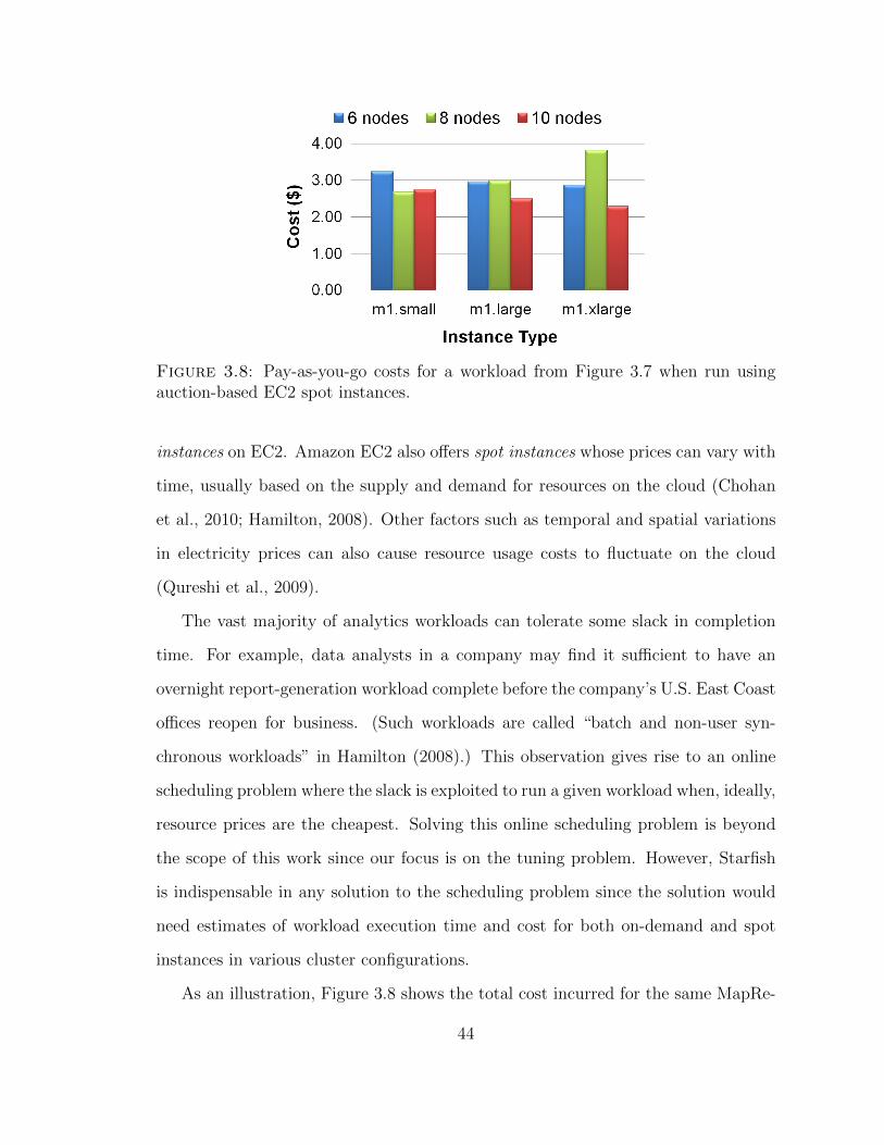
Figure 3.8: Pay-as-you-go costs for a workload from Figure 3.7 when run usingauction-based EC2 spot instances.
instances on EC2. Amazon EC2 also offers spot instances whose prices can vary with
time, usually based on the supply and demand for resources on the cloud (Chohan
et al., 2010; Hamilton, 2008). Other factors such as temporal and spatial variations
in electricity prices can also cause resource usage costs to fluctuate on the cloud
(Qureshi et al., 2009).
The vast majority of analytics workloads can tolerate some slack in completion
time. For example, data analysts in a company may find it sufficient to have an
overnight report-generation workload complete before the company’s U.S. East Coast
offices reopen for business. (Such workloads are called “batch and non-user syn-
chronous workloads” in Hamilton (2008).) This observation gives rise to an online
scheduling problem where the slack is exploited to run a given workload when, ideally,
resource prices are the cheapest. Solving this online scheduling problem is beyond
the scope of this work since our focus is on the tuning problem. However, Starfish
is indispensable in any solution to the scheduling problem since the solution would
need estimates of workload execution time and cost for both on-demand and spot
instances in various cluster configurations.
As an illustration, Figure 3.8 shows the total cost incurred for the same MapRe-
44
duce workload from Figure 3.7 when nodes of the EC2 spot instance type shown
were used to run the workload around 6.00 AM Eastern Time. The pricing model
used to compute the total cost in this case is:
total cost “num hours
ÿ
i“0
cost phpiq ˆ num nodes (3.2)
The summation here is over the number of hours of execution, with cost phpiq rep-
resenting the price charged per node type used in the cluster for the ith hour. By
comparing Figure 3.7(b) with Figure 3.8, it is clear that execution costs for the same
workload can differ significantly across different choices for the cluster resources used.
45
4
Dynamic Profiling of MapReduce Workloads
The high-level goal of dynamic profiling in Starfish is to collect run-time monitoring
information efficiently during the execution of a MapReduce job (recall Section 2.2.1).
Starfish uses dynamic profiling to build a job profile, which is a concise representation
of the job’s execution. There are some key challenges that Starfish needs to address
with respect to what, how, and when to profile.
First, we need to collect both dataflow and cost information during job execution.
Little knowledge about the input data may be available before the job is submitted.
Keys and values are often extracted dynamically from the input data by the map
function, so schema and statistics about the data may be unknown. In addition,
map and reduce functions are usually written in programming languages like Java,
Python, and C++ that are not restrictive or declarative like SQL. Hence, we need
to carefully observe the run-time cost of these functions, as well as how they process
the data.
Collecting fine-grained monitoring information efficiently and noninvasively is an-
other key challenge. We have chosen to use dynamic instrumentation to collect this
information from unmodified MapReduce programs. The dynamic nature means
46
that monitoring can be turned on or off on demand; an appealing property in pro-
duction deployments. Dynamic instrumentation has the added advantage that no
changes are needed to the MapReduce system’s source code (the Hadoop system in
our specific case). As a result, we leverage all past investments as well as potential
future enhancements to the MapReduce system.
Finally, the dynamic nature of profiling creates a need for investing some re-
sources upfront—i.e., before the actual job execution starts—to collect the neces-
sary information. However, many MapReduce programs are written once and run
many times over their lifetime (usually on different datasets). Programs for Extract-
Transform-Load (ETL) and report generation are good examples. Properties of such
programs as well as good configuration settings for them can be learned over time in
the spirit of learning optimizers like Leo (Stillger et al., 2001). For ad-hoc MapRe-
duce programs, we employ sampling techniques for collecting approximate profiling
information quickly.
4.1 Job and Workflow Profiles
A MapReduce job profile is a vector of fields where each field captures some unique
aspect of dataflow or cost during a MapReduce job execution at the task level or
the phase1 level within tasks. Including information at the fine granularity of phases
within tasks is crucial to the accuracy of decisions made by the What-if Engine and
the Cost-based Optimizers. We partition the fields in a profile into four categories,
described next. The rationale for this categorization will become clear in Chapter 6
when we describe how a virtual profile is estimated for a hypothetical job (without
actually running the job).
1 Recall the phases of MapReduce job execution discussed in Section 3.1
47
Table 4.1: Dataflow fields in the job profile. d, r, and c denote respectively inputdata properties, cluster resource properties, and configuration parameter settings.
Abbreviation Profile Field (All fields, unless Depends Onotherwise stated, represent d r cinformation at the level of tasks)
dNumMappers Number of map tasks in the job X XdNumReducers Number of reduce tasks in the job XdMapInRecs Map input records X XdMapInBytes Map input bytes X XdMapOutRecs Map output records X XdMapOutBytes Map output bytes X XdNumSpills Number of spills X XdSpillBufferRecs Number of records in buffer per spill X XdSpillBufferSize Total size of records in buffer per spill X XdSpillFileRecs Number of records in spill file X XdSpillFileSize Size of a spill file X XdNumRecsSpilled Total spilled records X XdNumMergePasses Number of merge rounds X XdShuffleSize Total shuffle size X XdReduceInGroups Reduce input groups (unique keys) X XdReduceInRecs Reduce input records X XdReduceInBytes Reduce input bytes X XdReduceOutRecs Reduce output records X XdReduceOutBytes Reduce output bytes X XdCombineInRecs Combine input records X XdCombineOutRecs Combine output records X XdLocalBytesRead Bytes read from local file system X XdLocalBytesWritten Bytes written to local file system X XdHdfsBytesRead Bytes read from HDFS X XdHdfsBytesWritten Bytes written to HDFS X X
• Dataflow fields capture information about the amount of data, both in terms
of bytes as well as records (key-value pairs), flowing through the different tasks
and phases of a MapReduce job execution. Some example fields are the number
of map output records and the amount of bytes shuffled among the map and
reduce tasks. Table 4.1 lists all the dataflow fields in a profile.
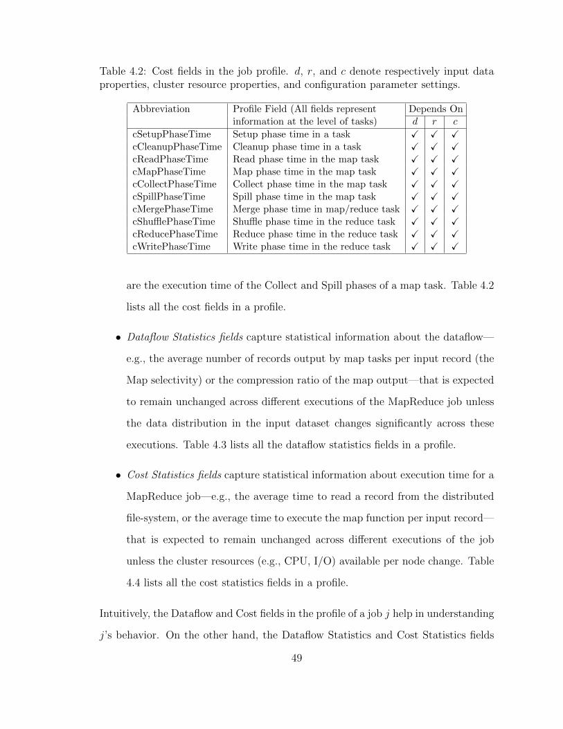
• Cost fields capture information about execution time at the level of tasks and
phases within the tasks for a MapReduce job execution. Some example fields
48
Table 4.2: Cost fields in the job profile. d, r, and c denote respectively input dataproperties, cluster resource properties, and configuration parameter settings.
Abbreviation Profile Field (All fields represent Depends Oninformation at the level of tasks) d r c
cSetupPhaseTime Setup phase time in a task X X XcCleanupPhaseTime Cleanup phase time in a task X X XcReadPhaseTime Read phase time in the map task X X XcMapPhaseTime Map phase time in the map task X X XcCollectPhaseTime Collect phase time in the map task X X XcSpillPhaseTime Spill phase time in the map task X X XcMergePhaseTime Merge phase time in map/reduce task X X XcShufflePhaseTime Shuffle phase time in the reduce task X X XcReducePhaseTime Reduce phase time in the reduce task X X XcWritePhaseTime Write phase time in the reduce task X X X
are the execution time of the Collect and Spill phases of a map task. Table 4.2
lists all the cost fields in a profile.
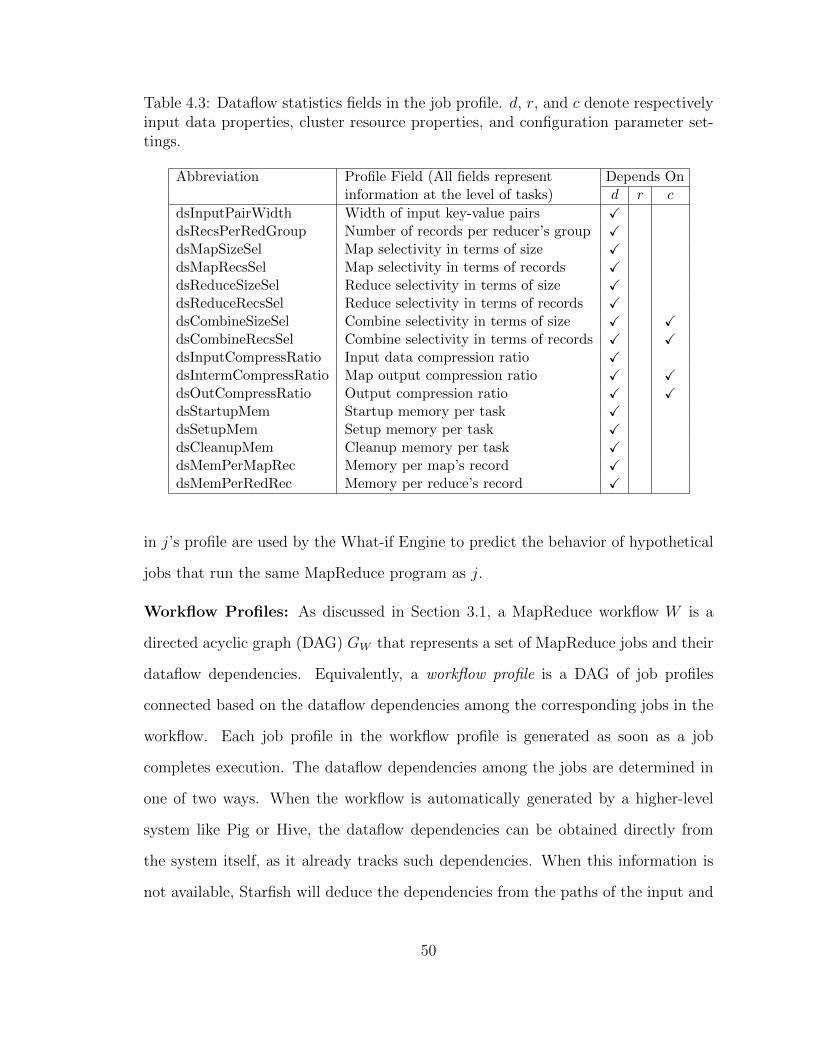
• Dataflow Statistics fields capture statistical information about the dataflow—
e.g., the average number of records output by map tasks per input record (the
Map selectivity) or the compression ratio of the map output—that is expected
to remain unchanged across different executions of the MapReduce job unless
the data distribution in the input dataset changes significantly across these
executions. Table 4.3 lists all the dataflow statistics fields in a profile.
• Cost Statistics fields capture statistical information about execution time for a
MapReduce job—e.g., the average time to read a record from the distributed
file-system, or the average time to execute the map function per input record—
that is expected to remain unchanged across different executions of the job
unless the cluster resources (e.g., CPU, I/O) available per node change. Table
4.4 lists all the cost statistics fields in a profile.
Intuitively, the Dataflow and Cost fields in the profile of a job j help in understanding
j’s behavior. On the other hand, the Dataflow Statistics and Cost Statistics fields
49
Table 4.3: Dataflow statistics fields in the job profile. d, r, and c denote respectivelyinput data properties, cluster resource properties, and configuration parameter set-tings.
Abbreviation Profile Field (All fields represent Depends Oninformation at the level of tasks) d r c
dsInputPairWidth Width of input key-value pairs XdsRecsPerRedGroup Number of records per reducer’s group XdsMapSizeSel Map selectivity in terms of size XdsMapRecsSel Map selectivity in terms of records XdsReduceSizeSel Reduce selectivity in terms of size XdsReduceRecsSel Reduce selectivity in terms of records XdsCombineSizeSel Combine selectivity in terms of size X XdsCombineRecsSel Combine selectivity in terms of records X XdsInputCompressRatio Input data compression ratio XdsIntermCompressRatio Map output compression ratio X XdsOutCompressRatio Output compression ratio X XdsStartupMem Startup memory per task XdsSetupMem Setup memory per task XdsCleanupMem Cleanup memory per task XdsMemPerMapRec Memory per map’s record XdsMemPerRedRec Memory per reduce’s record X
in j’s profile are used by the What-if Engine to predict the behavior of hypothetical
jobs that run the same MapReduce program as j.
Workflow Profiles: As discussed in Section 3.1, a MapReduce workflow W is a
directed acyclic graph (DAG) GW that represents a set of MapReduce jobs and their
dataflow dependencies. Equivalently, a workflow profile is a DAG of job profiles
connected based on the dataflow dependencies among the corresponding jobs in the
workflow. Each job profile in the workflow profile is generated as soon as a job
completes execution. The dataflow dependencies among the jobs are determined in
one of two ways. When the workflow is automatically generated by a higher-level
system like Pig or Hive, the dataflow dependencies can be obtained directly from
the system itself, as it already tracks such dependencies. When this information is
not available, Starfish will deduce the dependencies from the paths of the input and
50
Table 4.4: Cost statistics fields in the job profile. d, r, and c denote respectively inputdata properties, cluster resource properties, and configuration parameter settings.
Abbreviation Profile Field (All fields represent information Depends Onat the level of tasks) d r c
csHdfsReadCost I/O cost for reading from HDFS per byte XcsHdfsWriteCost I/O cost for writing to HDFS per byte XcsLocalIOReadCost I/O cost for reading from local disk per byte XcsLocalIOWriteCost I/O cost for writing to local disk per byte XcsNetworkCost Cost for network transfer per byte XcsMapCPUCost CPU cost for executing the Mapper per record XcsReduceCPUCost CPU cost for executing the Reducer per record XcsCombineCPUCost CPU cost for executing the Combiner per record XcsPartitionCPUCost CPU cost for partitioning per record XcsSerdeCPUCost CPU cost for serializing/deserializing per record XcsSortCPUCost CPU cost for sorting per record XcsMergeCPUCost CPU cost for merging per record XcsInUncomprCPUCost CPU cost for uncompr/ing the input per byte XcsIntermUncomCPUCost CPU cost for uncompr/ing map output per byte X XcsIntermComCPUCost CPU cost for compressing map output per byte X XcsOutComprCPUCost CPU cost for compressing the output per byte X XcsSetupCPUCost CPU cost of setting up a task XcsCleanupCPUCost CPU cost of cleaning up a task X
output data processed and generated by each job in the workflow.
Information contained in a workflow profile can be used to reconstruct the entire
execution of the MapReduce jobs after their completion, in order to better under-
stand and analyze their overall behavior as well as the various dependencies among
them. In addition, as we will see in Chapter 6, the workflow profile is utilized to
answer hypothetical what-if questions regarding the behavior of the workflow under
different scenarios.
Job and workflow profiles are a very powerful abstraction for representing the
execution of any arbitrary MapReduce program or any query expressed in a higher-
level language like Pig Latin or HiveQL. Apart from using profiles in answering
what-if questions and automatically recommending configuration parameter settings,
the profiles also help in understanding the job behavior as well as in diagnosing
bottlenecks during job execution.
51
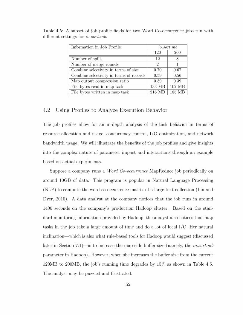
Table 4.5: A subset of job profile fields for two Word Co-occurrence jobs run withdifferent settings for io.sort.mb.
Information in Job Profile io.sort.mb120 200
Number of spills 12 8
Number of merge rounds 2 1
Combine selectivity in terms of size 0.70 0.67
Combine selectivity in terms of records 0.59 0.56
Map output compression ratio 0.39 0.39
File bytes read in map task 133 MB 102 MB
File bytes written in map task 216 MB 185 MB
4.2 Using Profiles to Analyze Execution Behavior
The job profiles allow for an in-depth analysis of the task behavior in terms of
resource allocation and usage, concurrency control, I/O optimization, and network
bandwidth usage. We will illustrate the benefits of the job profiles and give insights
into the complex nature of parameter impact and interactions through an example
based on actual experiments.
Suppose a company runs a Word Co-occurrence MapReduce job periodically on
around 10GB of data. This program is popular in Natural Language Processing
(NLP) to compute the word co-occurrence matrix of a large text collection (Lin and
Dyer, 2010). A data analyst at the company notices that the job runs in around
1400 seconds on the company’s production Hadoop cluster. Based on the stan-
dard monitoring information provided by Hadoop, the analyst also notices that map
tasks in the job take a large amount of time and do a lot of local I/O. Her natural
inclination—which is also what rule-based tools for Hadoop would suggest (discussed
later in Section 7.1)—is to increase the map-side buffer size (namely, the io.sort.mb
parameter in Hadoop). However, when she increases the buffer size from the current
120MB to 200MB, the job’s running time degrades by 15% as shown in Table 4.5.
The analyst may be puzzled and frustrated.
52
Figure 4.1: Map and reduce time breakdown for two Word Co-occurrence jobs runwith different settings for io.sort.mb.
By using our Profiler to collect job profiles, the data analyst can visualize the
task-level and phase-level Cost (timing) fields as shown in Figure 4.1. It is obvious
immediately that the performance degradation is due to a change in map perfor-
mance; and the biggest contributor is the change in the Spill phase’s cost. The
analyst can drill down to the values of the relevant profile fields, which we show in
Figure 4.1. The values shown report the average across all map tasks.
The interesting observation from Figure 4.1 is that changing the map-side buffer
size from 120MB to 200MB improves all aspects of local I/O in map task execution:
the number of spills reduced from 12 to 8, the number of merges reduced from 2 to
1, and the Combine function became more selective. Overall, the amount of local
I/O (reads and writes combined) per map task went down from 349MB to 287MB.
However, the overall performance still degraded.
To further understand the job behavior, we run the Word Co-occurrence job with
different settings of the map-side buffer size (io.sort.mb). Figure 4.2 shows the overall
map execution time, and the time spent in the map-side Spill and Merge phases, from
our runs. The input data and cluster resources are identical for the runs. Notice
the map-side buffer size’s nonlinear effect on cost, which comes from an interesting
tradeoff: a larger buffer lowers overall I/O size and cost (Figure 4.1), but increases
53
Figure 4.2: Total map execution time, Spill time, and Merge time for a represen-tative Word Co-occurrence map task as we vary the setting of io.sort.mb.
the computational cost nonlinearly because of sorting.
Figure 4.2 also shows the corresponding execution times as predicted by Starfish’s
What-if Engine. We observe that the What-if Engine correctly captures the un-
derlying nonlinear effect that caused this performance degradation; enabling the
Cost-based Optimizer to find the optimal setting of the map-side buffer size. The
fairly uniform gap between the actual and predicted costs is due to overhead added
by BTrace (our profiling tool discussed below) while measuring function timings at
nanosecond granularities.2 Because of its uniformity, the gap does not affect the ac-
curacy of what-if analysis which, by design, is about relative changes in performance.
4.3 Generating Profiles via Measurement
A job profile (and, by extension, a workflow profile) is generated by one of two
methods. We will first describe how the Profiler generates profiles from scratch by
collecting monitoring data during full or partial job execution. The second method
is by estimation, which does not require the job to be run. Profiles generated by this
method are called virtual profiles. The What-if Engine is responsible for generating
2 We expect to close this gap using commercial Java profilers that have demonstrated vastly loweroverheads than BTrace (Louth, 2009).
54
virtual profiles as part of answering a what-if question (discussed in Chapter 6).
Monitoring through dynamic instrumentation: When a user-specified MapRe-
duce program p is run, the MapReduce framework is responsible for invoking the map,
reduce, and other functions in p. This property is used by the Profiler to collect run-
time monitoring data from unmodified programs running on the MapReduce frame-
work, using dynamic instrumentation. Dynamic instrumentation is now a popular
technique used to understand, debug, and optimize complex systems (Cantrill et al.,
2004). The Profiler applies dynamic instrumentation to the MapReduce framework—
not to the MapReduce program p—by specifying a set of event-condition-action
(ECA) rules.
The space of possible events in the ECA rules corresponds to events arising during
program execution, such as entry or exit from functions, memory allocation, and
system calls to the operating system. If the condition associated with the event
holds when the event fires, then the associated action is invoked. An action can
involve, for example, getting the duration of a function call, examining the memory
state, or counting the number of bytes transferred.
The current implementation of the Profiler for the Hadoop MapReduce framework
uses the BTrace dynamic instrumentation tool for Java (BTrace, 2012). To collect
raw monitoring data for a program being run by Hadoop, the Profiler uses ECA rules
(also specified in Java) to dynamically instrument the execution of selected Java
classes internal to Hadoop. Under the covers, dynamic instrumentation intercepts
the corresponding Java class bytecodes as they are executed, and injects additional
bytecodes to run the associated actions in the ECA rules.
Apart from Java, Hadoop can run a MapReduce program written in various
programming languages such as Python, R, or Ruby using Streaming, or C++ using
Pipes (White, 2010). Hadoop executes Streaming and Pipes jobs through special map
55
and reduce tasks that each communicate with an external process to run the user-
specified map and reduce functions (White, 2010). Since the Profiler instruments
only the MapReduce framework, not the user-written programs, profiling works ir-
respective of the programming language in which the program is written.
From raw monitoring data to profile fields: The raw monitoring data collected
through dynamic instrumentation of job execution at the task and phase levels in-
cludes record and byte counters, timings, and resource usage information. For ex-
ample, during each spill, the exit point of the sort function is instrumented to collect
the sort duration as well as the number of bytes and records sorted. A series of
post-processing steps involving aggregation and extraction of statistical properties
is applied to the raw data in order to generate the various fields in the job profile
(recall Section 4.1).
The raw monitoring data collected from each profiled map or reduce task is first
processed to generate the fields in a task profile. For example, the raw sort timings are
added as part of the overall spill time, whereas the Combine selectivity from each spill
is averaged to get the task’s Combine selectivity. The map task profiles are further
processed to give one representative map task profile for each logical input to the
MapReduce program. For example, a Sort program accepts a single logical input (be
it a single file, a directory, or a set of files), while a two-way Join accepts two logical
inputs. The reduce task profiles are processed into one representative reduce task
profile. The representative map task profile(s) and the reduce task profile together
constitute the job profile.
The aggregated dataflow and cost fields in the profiles provide a global view
of the job execution, whereas the aggregated dataflow and cost statistics fields are
essential for estimating the profile fields for hypothetical jobs (discussed in Chapter
6. Apart from point-value fields, the Profiler can potentially be used to collect all
56
individual key-value flows across tasks to compute key-value distributions for input,
intermediate, and output data. Such information opens up new tuning possibilities,
especially for higher-level systems like Pig and Hive. For example, Pig could use
information about intermediate data distributions for automatically selecting the
partitioning function or appropriate join algorithm.
Current approaches to profiling in Hadoop: Monitoring facilities in Hadoop—
which include logging, counters, and metrics—provide historical data that can be
used to monitor whether the cluster is providing the expected level of performance,
and to help with debugging and performance tuning (White, 2010).
Hadoop counters are a useful channel for gathering statistics about a job for
quality control, application-level statistics, and problem diagnosis. Hadoop contains
a set of built-in counters measuring task-level statistics, like the number of input
and output records for each task, and the number of bytes read and written to the
file-systems. Counters are collected for MapReduce tasks and aggregated for the
whole job. In addition, Hadoop offers support for user-defined counters. Counters
are similar to the Dataflow fields in a job profile, and can be useful in setting some job
configuration parameters. For example, the total number of records spilled to disk
may indicate that some memory-related parameters in the map task need adjustment;
but the user cannot automatically know which parameters to adjust or how to adjust
them to improve the job’s performance.
The HDFS and MapReduce daemons in Hadoop expose runtime metrics about
events and measurements (White, 2010). For example, HDFS Datanodes3 collect
metrics recording the number of bytes written, the number of blocks replicated,
and the number of read requests in a node. Even though metrics have similar uses
to counters, they represent cluster-level information and their target audience is
3 Datanodes are HDFS entities run on each slave node in the cluster and are responsible for storingand retrieving file blocks from each node.
57
system administrators, not regular users. In addition, Hadoop metrics have a lot of
dependencies on third party software and libraries as they have to be analyzed by
cluster monitoring systems like Ganglia or Nagios.
Information similar to counters and metrics forms only a fraction of the infor-
mation in the job profiles collected by the Profiler. Apart from an extensive list
of counters, the job profile contains (i) statistical information like map and reduce
selectivities, (ii) quantitative costs for executing user-provided functions like maps,
reduces, and combiners, and (iii) time spent in the various task phases.
4.4 Task-level Sampling to Generate Approximate Profiles
Another valuable feature of dynamic instrumentation is that it can be turned on
or off seamlessly at run-time, incurring zero overhead when turned off. However, it
does cause some task slowdown when turned on. We have implemented two tech-
niques that use task-level sampling in order to generate approximate job profiles
while keeping the run-time overhead low:
1. If the intent is to profile a job j during a regular run of j on the production
cluster, then the Profiler can collect task profiles for only a sample of j’s tasks.
2. If the intent is to collect a job profile for j as quickly as possible, then the
Profiler can selectively execute (and profile) only a sample of j’s tasks.
Consider a job with 100 map tasks. With the first approach and a sampling per-
centage of 10%, all 100 tasks will be run, but only 10 of them will have dynamic
instrumentation turned on. In contrast, the second approach will run (and profile)
only 10 of the 100 tasks.
In order to examine the relationship between task-level sampling and the ability
to generate job profiles based on which Starfish can make fairly accurate decisions,
58
Figure 4.3: (a) Overhead to measure the (approximate) profile, and (b) corre-sponding speedup given by Starfish as the percentage of profiled tasks is varied forWord Co-occurrence and TeraSort MapReduce jobs.
we performed the following experiment. We ran and profiled Word Co-occurrence
(a CPU-intensive job) and TeraSort (an I/O-intensive job) on a 16-node Hadoop
cluster with c1.medium EC2 nodes, while enabling profiling for only a sample of the
tasks in each job. We then used the generated (approximate) job profiles to get
recommendations for parameter settings from Starfish. (Understanding the details
of how Starfish works at this point is not needed for appreciating the results.)
As we vary the percentage of profiled tasks in each job, Figure 4.3(a) shows the
profiling overhead compared against the same job run with profiling turned off. For
59
both MapReduce jobs, as the percentage of profiled tasks increases, the overhead
added to the job’s running time also increases (as expected). Profiling all the map
and reduce tasks in each job adds around 15% to 20% overhead to the job’s execution
time. It is interesting to note that the profiling overhead varies significantly between
the two jobs. The magnitude of the profiling overhead depends on whether the job
is CPU-bound, uses a combine function, or uses compression, as well as on the job
configuration settings.
Figure 4.3(b) shows the speedup achieved in job execution time by the Starfish-
suggested settings over rule-based settings as the percentage of profiled tasks used to
generate the job profile is varied. In most cases, the settings suggested by Starfish
led to nearly the same job performance improvements; showing that the Starfish’s
effectiveness in finding good configuration settings does not require that all tasks be
profiled. In fact, by profiling just 10% of the tasks, Starfish can often achieve the
same speedup as by profiling 100% of the tasks.
It is particularly encouraging to note that by profiling just 1% of the tasks—in this
specific cases, profiling only one map and one reduce task—with near-zero overhead
on job execution, Starfish finds configuration settings that still provide a speedup over
the jobs run with rule-based settings. We have repeated this experiment with a large
number of different MapReduce programs and, in most cases, the settings suggested
by Starfish using sampling led to nearly the same job performance improvements like
above. Therefore, by profiling only a small fraction of the tasks, we can keep the
overhead low while achieving high degrees of accuracy in the collected information.
60
5
A Declarative Query Interface to AccessPerformance Predictors and Optimizers
Starfish is a self-tuning system for running analytics workloads on Big Data. As
described in Section 2.2.1 and illustrated in Figure 2.1, Starfish is built on the Hadoop
platform. Starfish interposes itself between Hadoop and higher-level clients (e.g.,
Pig, Hive, Oozie, and command-line interfaces) to submit MapReduce jobs. These
Hadoop clients will now submit workloads—which can vary from a single MapReduce
job, to a workflow of MapReduce jobs, and to a collection of multiple workflows—
directly to Starfish. Starfish provides a wide range of features to the users, including,
but not limited to, the following:
1. The user has the option to either execute the MapReduce workload on the
Hadoop cluster as is or to enable the collection of profiling information during
execution. In the former case, the workload will execute with zero overhead and
Starfish will get access to Hadoop’s default logs and counters; whereas in the
latter case, Starfish will generate fine-grained job and workflow profiles. This
61
information is organized, stored, and managed by Starfish’s Data Manager1.
2. The information collected by the Profiler helps in understanding the job behav-
ior as well as in diagnosing bottlenecks during job execution. For this purpose,
Starfish provides both a command-line and a graphical user interface for ex-
ploring and analyzing the collected data. The profiles are also required for
Starfish to predict and optimize the performance of MapReduce workloads.
3. The What-if Engine can predict the performance of a MapReduce job j (or
workflow W ), allowing the user to study the effects of configuration parameters,
cluster resources, and input data on the performance of j (or W ); without
actually running j (or W ).
4. The Job and Workflow Optimizers can find the optimal configuration settings
for j (or W ), and can also help understand why the current settings are (pos-
sibly) suboptimal.
5. The Cluster Resource Optimizer can find the optimal number of nodes and
node types to use for a MapReduce workload given objectives and constraints
on execution time and/or cost.
At the same time, we want Starfish to be usable in environments where workloads are
run directly on Hadoop without going through Starfish. For this purpose, Starfish
can be run in a special recommendation mode. In this mode, Starfish uses its tuning
features to only recommend good configurations instead of running the workload
with these configurations as Starfish would do in its normal usage mode.
Predicting the performance of MapReduce workloads, finding MapReduce pa-
rameter settings, and determining the best cluster resources to use are instances of
workload tuning problems Starfish can solve. We have developed a declarative query
1 Recall the components in the Starfish architecture shown in Figure 2.2 in Section 2.2.1.
62
interface through which the users can express workload tuning queries. Starfish will
then provide reliable answers to these queries using an automated technique; provid-
ing nonexpert users with a good combination of cluster resource and job configuration
settings to meet their needs. The automated technique is based on a careful mix of
job profiling, estimation using black-box and white-box models, and simulation. Ap-
plications and users can also interact with this interface using a programmatic API
or using a graphical interface that forms part of the Starfish system’s Visualizer.
5.1 Declarative Interface to Express Workload Tuning Queries
A general tuning problem involves determining the cluster resources and MapReduce
job-level configuration settings to meet desired performance requirements on execu-
tion time and cost for a given analytic workload. Starfish provides a declarative
interface to express a range of tuning queries including those arising in the use cases
discussed in Section 3.4.
A tuning query specified using Starfish’s declarative query interface has four parts.
We discuss each of these parts in turn.
1. Specifying the workload: The workload specified in a tuning query consists of
MapReduce jobs, including both single jobs as well as jobs from multi-job workflows.
Each job j runs some MapReduce program p on input data d. A profile profppq has
to be given for p. profppq need not, and usually will not, correspond to the actual
job j = xp, d, r, cy that eventually runs p as part of the workload. If d is different
from the input data used while generating profppq, then the properties of d have
to be given. For user convenience, when d is actual data on a live cluster, Starfish
can collect the properties of d (and r) automatically from the cluster. The cluster
resources r and job configuration c to use in the actual execution of j are part of
separate specifications that involve search spaces, discussed next.
63
2. Specifying the search space for cluster resources r: Recall from Section 3.1
that the properties used to represent any cluster resources r include the number of
nodes, node type(s), and network topology of r, the number of map and reduce task
execution slots per node, and the maximum memory available per task execution
slot. A search space over the number of nodes and the node type to use in the
cluster is specified for r. This search space is specified as a nonempty set. It is the
responsibility of Starfish to find a suitable cluster resource configuration from this
search space that meets all other requirements in the query.
The search space for r will be a singleton set if the user is asking for performance
estimates for a specific (hypothetical or real) cluster that she has in mind. Use cases
1, 2, and 3 from Section 3.4 have this nature. For example, in use case 2, the user
currently has a cluster containing 10 EC2 nodes of the m1.large type. She wants
Starfish to estimate what the job’s execution time will be on a hypothetical cluster
containing 15 nodes of the same type.
The search space is nonsingleton—i.e., it specifies a space that contains more
than one candidate resource configuration—when the user wants Starfish to search
for a good configuration that meets her needs. In such cases, Starfish’s declarative
query interface gives the user considerable flexibility to define the search space for
cluster resources r. For example:
• An unsophisticated user can use the special “*” symbol to ask Starfish to use
its default search space for one or both of the node type and the number of
nodes.
• The user can restrict the search space to nodes of one or more selected types,
but ask Starfish to find the best number of nodes in the cluster.
Our current implementation of the Cluster Resource Optimizer does not include
the cluster’s network topology in the search space. This limitation, which can be
64
removed in the future, is driven partly by a practical consideration: most current
cloud providers hide the underlying network topology from clients. The Hadoop
clusters that we run on EC2 are configured as per the single-rack network topology
used by default in Hadoop.
The Hadoop cluster-wide configuration parameters—namely, the number of map
and reduce task execution slots per node, and the maximum memory available per
task execution slot—are also not included in the search space. Our empirical studies
indicate that good settings for these parameters are determined primarily by the
CPU (number of cores) and memory resources available per node in the cluster; so
we use empirically-determined fixed values per node type (these values are shown in
Table 6.3).2
3. Specifying the search space for job configurations c: Recall the space
of configuration parameter settings for MapReduce jobs presented in Section 3.1
and Table 3.1. A tuning query needs to specify the search space for configuration
parameters c that Starfish should consider for the given workload of MapReduce
jobs. Similar to the search space for cluster resources, the search space for c will be a
singleton set if the user is asking for performance estimates for a specific configuration
that she has in mind. Use case 2 from Section 3.4 has this nature.
It is much more common to specify a larger search space for c. The best setting of
configuration parameters depends strongly on the cluster resource configuration. For
the convenience of nonexpert users who often have no idea about the configuration
parameters, the special “*” symbol can be specified to ask Starfish to use its default
search space for c.
The Job and Workflow Optimizers in Starfish are responsible for searching effi-
ciently through the specified space of configuration parameter settings. Starfish uses
2 Anecdotal evidence from the industry suggests that memory-related misconfigurations are amajor cause of failures in Hadoop.
65
the Job and Workflow Optimizers in tandem with the Cluster Resource Optimizer
since the best job configuration will invariably change if the cluster resources change.
4. Specifying performance requirements: Execution time and cost are the two
performance metrics supported by Starfish. As part of a tuning query, a user can
choose to:
• Have estimated values output for one or both of these metrics.
• Optimize one of these metrics, possibly subject to a constraint on the other
metric. For example, optimizing monetary cost subject to an execution time
under 30 minutes.
5.2 Overview of How Starfish Answers a Workload Tuning Query
This section gives an overview of how Starfish answers a tuning query posed by a user
or application. Chapters 6 and 7 will describe the individual steps in more detail.
To simplify the discussion, we will use concrete examples arising from the use cases
described in Section 3.4.
1. Tuning job-level configuration parameter settings: Consider a MapReduce
job j = xp, d, r, cy that run on a 10-node Hadoop cluster using 20 reduce tasks. The
user is interested in the affect of the number of reduce tasks (one of the configuration
parameters) on the performance of the job. In this scenario, the user can ask for an
estimate of the execution time of job j1 = xp, d, r, c1y whose configuration c1 is the
same as c except that c1 specifies using 40 reduce tasks. The MapReduce program p,
input data d, and cluster resources r remain unchanged. A user can express this use
case as a tuning query Q1 using Starfish’s query interface described in Section 5.1.
The user will specify the following:
• The profile for the run of job j on the current Hadoop cluster. Chapter 4
66
described how the profile can be generated by measurement as part of an actual
job execution.
• The search space for cluster resources r is a singleton set that specifies the
current Hadoop cluster.
• The search space for the configuration parameter settings is also a singleton
set that specifies c1.
• The performance metric of interest is execution time.
Query Q1 maps directly to a what-if question that can be answered by the What-if
Engine. The What-if Engine will first estimate a virtual job profile for the hypothet-
ical job j1. This step uses a careful mix of white-box and black-box models. The
virtual profile is then used in a simulation step to estimate how the hypothetical
job j1 will execute. The answer to the what-if question is computed based on the
estimated execution. Note that job j1 is never run during this process. Chapter 6
explains the overall prediction process in detail.
A what-if question can involve multiple jobs in a workload. In this case, all the
virtual job profiles are generated, and then input to the simulation step.
2. Tuning the cluster size for elastic workloads: Suppose a MapReduce job j
takes three hours to finish on a 10-node Hadoop cluster of EC2 nodes of the m1.large
type. The user who controls the cluster wants to know by how much the execution
time of the job will reduce if five more m1.large nodes are added to the cluster. This
use case is expressed as a tuning query Q2 by specifying the following:
• The profile for the run of j on 10 m1.large EC2 nodes.
• The search space for cluster resources r is a singleton set that specifies 15 EC2
nodes of the (same) m1.large type.
67
• The search space for the configuration parameter settings c is also a singleton
set that specifies the same job configuration as for the 10-node cluster.
• The performance metric of interest is execution time.
The above specification of query Q2 gives Starfish a profile for a job j = xp, d, r1, cy.
The desired answer is the estimate of execution time for a hypothetical job j1 =
xp, d, r2, cy. Job j1 runs the same program p on the same data d and MapReduce
configuration c as job j. However, the cluster resources used are different between
j and j1, i.e., r1 ‰ r2. Similar to Query Q1, Query Q2 maps directly to a what-if
question. However, the answer to Q2 involves estimating the performance of j1 on a
hypothetical cluster instead of a real one.
3. Planning for workload transition from a development cluster to pro-
duction: To express this use case as a tuning query Q3, a user will specify the
following:
• A job profile collected on the development cluster for the program p of interest.
This profile may have been collected by direct measurement when p was run
on a (scaled down) sample of the production data on which the program has to
be run on the production cluster. In this case, the properties of the production
data dprod will have to be provided.
• The search space for cluster resources r is a singleton set that gives the prop-
erties of the production cluster, denoted rprod.
• Note that the developer wants Starfish to find the best job configuration to run
the job on the production cluster. Thus, the search space for the configuration
parameter settings c is specified as “*” so that Starfish will consider the full
space in an efficient fashion.
68
• The performance metric of interest is execution time.
To process query Q3, Starfish will invoke the cost-based Job Optimizer to efficiently
enumerate and search through the high-dimensional space of configuration parameter
settings. The Job Optimizer will consider hypothetical configurations cp1q, cp2q, . . .
cpiq, . . ., cpnq, making calls to the What-if Engine to get the estimated execution
time of each of the corresponding hypothetical jobs jpiq = xp, dprod, rprod, cpiqy. The
configuration cpoptq found in this process with the least execution time will be output
as the query result; the details of the efficient search process are given in Chapter 7.
4. Cluster provisioning under multiple objectives: This use case differs from
the earlier use cases in two main ways. First, the search space for cluster resources
is not a singleton set any more. Second, the performance requirements demand
optimization of monetary cost, while specifying a constraint on the execution time.
(Note that optimizing the execution time with a constraint on monetary cost is also
supported.) A user will specify the following:
• A job profile collected on a Hadoop cluster with 6 nodes of m1.large EC2 type
for the program p of interest.
• The search space for cluster resources r specifies “*” so that Starfish will con-
sider all available instance types and cluster sizes.
• The search space for the configuration parameter settings c is also specified as
“*” so that Starfish will consider the full space in an efficient fashion.
• The objective is to minimize the monetary cost while the job runs in less than
2 hours.
The Cluster Resource Optimizer and the Job Optimizer will be used in tandem to
enumerate and search over the space of cluster resources and job configurations;
69
while making calls to the What-if Engine to get estimates of execution time and cost
for hypothetical jobs jpi,jq = xp, d, rpiq, cpjqy. The combination xr,cy poptq found in this
process that gives the least monetory cost while meeting the constraint on execution
time will be output as the query result.
5.3 Starfish Visualizer
The Visualizer forms the graphical user interface to Starfish. Users employ the
Visualizer to (a) get a deep understanding of a MapReduce job’s behavior dur-
ing execution, (b) ask hypothetical questions on how the job behavior will change
when parameter settings, cluster resources, or input data properties change, and
(c) ultimately optimize the job. Hence, we categorize the core functionalities of
the Visualizer into Job Analysis, What-if Analysis, and Job Optimization. For each
functionality, the Visualizer offers five different views:
1. Timeline views, used to visualize the progress of job execution at the task level.
2. Data Skew views, used to identify the presence of data skew in the input and
output data of map and reduce tasks.
3. Data Flow views, used to visualize the flow of data among the nodes of a
Hadoop cluster, and between the map and reduce tasks of a job.
4. Profile views, used to show the detailed information exposed by the job profiles,
including the phase timings within the tasks.
5. Settings views, used to list the configuration parameter settings, cluster re-
sources, and the input data properties during job execution.
We will demonstrate the Visualizer’s functionalities in order, and show how the user
can obtain deep insights into a job’s performance from each view in each case.
70
Figure 5.1: Screenshot from the Starfish Visualizer showing the execution timelineof the map and reduce tasks of a MapReduce job running on a Hadoop cluster. Auser can quickly get useful information such as the number of map and reduce wavesor the presence of variance in the task execution times.
Job Analysis: Recall from Section 4.3 that when a MapReduce job executes on a
Hadoop cluster, the Profiler collects a wealth of information including logs, counters,
and profiling data. Figure 5.13 shows the execution timeline of map and reduce tasks
that ran during a MapReduce job execution. The user can get information such as
how many tasks were running at any point in time on each node, when each task
started and ended, or how many map or reduce waves occurred during job execution.
The user is able to quickly spot any high variance in the task execution times, and
discover potential load-balancing issues. Moreover, Timeline views can be used to
compare different executions of the same job run at different times or with different
3 All figures are actual screenshots from the Starfish Visualizer.
71
Figure 5.2: Screenshot from the Starfish Visualizer showing a histogram of themap output data size per map task that can be used to identify data skew. Thisparticular histogram shows that 33% of the map tasks output about 2x more datathan the other map tasks.
parameter settings. Comparison of timelines shows whether the job behavior changed
over time and helps understand the impact of changing parameter settings on job
execution.
While the Timeline views are useful in identifying computational skew, the Data
Skew views (shown in Figure 5.2) can readily help identify the presence of skew in
the data consumed and produced by the map and reduce tasks. Data skew in the
reduce tasks usually indicates a strong need for a better partitioning function in the
current MapReduce job. Data skew in the map tasks corresponds to properties of
the input data, and may indicate the need for a better partitioning function in the
producer job that generates the input data.
72
Figure 5.3: Screenshot from the Starfish Visualizer showing a visual representationof the data flow among the Hadoop nodes during a MapReduce job execution. Theprovided Video mode allows a user to inspect how data was transfered among thenodes of the cluster as time went by.
The Data Skew views are complemented by the Data Flow views used to identify
data skew across the Hadoop nodes caused during the Shuffle phase of the MapRe-
duce job execution. Figure 5.3 presents the data flow among some cluster nodes
during the execution of a MapReduce job. The thickness of each line is proportional
to the amount of data that was shuffled between the corresponding nodes. The user
also has the ability to specify a set of filter conditions (see the left side of Figure
5.3) that allows her to zoom in on a subset of nodes or on the large data transfers.
An important feature of the Visualizer is the Video mode that allows users to play
back a job execution from the past. Using the Video mode, the user can inspect how
data was processed and transfered between the map and reduce tasks of the job, and
73
Figure 5.4: Screenshot from the Starfish Visualizer showing the map and reducetime breakdown from the virtual profile of a MapReduce job. A user here can quicklyspot that the time spent shuffling the map output data to the reduce tasks contributesthe most to the total execution time.
among nodes and racks of the cluster, as time went by.
The Profile views help visualize the job profiles, namely, the information exposed
by the profile fields at the fine granularity of phases within the map and reduce tasks
of a job; allowing for an in-depth analysis of task behavior during execution. For ex-
ample, Figure 5.4 displays the breakdown of time spent on average in each map and
reduce task. The Profile views also form an excellent way of diagnosing bottlenecks
during task execution. From the visualization shown in Figure 5.4, even a nonex-
pert user can spot that the time spent shuffling the map output data to the reduce
tasks contributes the most to the total execution time; indicating that the corre-
sponding configuration parameters (e.g., mapred.job.shuffle.input.buffer.percent and
74
Figure 5.5: Screenshot from the Starfish Visualizer showing the optimal configu-ration parameter settings found by the Job Optimizer, as well as cluster and inputdata properties. The user also has the option of importing or exporting any of theabove settings and properties in XML format.
mapred.job.shuffle.merge.percent from Table 3.1) have settings that are potentially
suboptimal.
Finally, the Settings view (see Figure 5.5) lists the most important Hadoop con-
figuration parameters used during the execution of a MapReduce job, as well as the
cluster setup and input data properties. The cluster setup is summarized as the
number of nodes, the average number of map and reduce slots per node, and the
memory available for each task execution. The input data properties include the size
and compression of each input split processed by a single map task. The user also
has the option of importing or exporting any of the above settings in XML format.
75
What-if Analysis: The second core functionality provided by the Starfish Visual-
izer is the ability to answer hypothetical questions about the behavior of a MapRe-
duce job when run under different settings. This functionality allows users to study
and understand the impact of configuration parameter settings, cluster resources,
and input data properties on the performance of a MapReduce job.
For instance, the user can ask a what-if question of the form: “How will the
execution time of a job change if the number of reduce tasks is doubled?” The
user can then use the Timeline view to visualize what the execution of the job will
look like under the new settings, and compare it to the current job execution. By
varying the number of reducers (or any other configuration parameter), the user can
determine the impact of changing that parameter on the job execution. Under the
hood, the Visualizer invokes the What-if Engine to generate a virtual job profile for
the job in the hypothetical setting.
Furthermore, the user can investigate the behavior of MapReduce jobs when
changing the cluster setup or the input specification. This functionality is useful in
two scenarios. First, many organizations run the same MapReduce programs over
multiple datasets with similar data distribution, but different sizes. For example, the
same report-generation MapReduce program may be used to generate daily, weekly,
and monthly reports. Or, the daily log data collected and processed may be larger
for a weekday than the data for the weekend. By modifying the input specification,
the user can ask what-if questions on the job behavior when the job is run using
datasets of different sizes.
Another common use-case is the presence of a development cluster for generating
job profiles. In many companies, developers use a small development cluster for
testing and debugging MapReduce programs over small (representative) datasets
before running the programs, possibly multiple times, on the production cluster.
Again, the user can modify the cluster setup in order to determine in advance how
76
the jobs will behave on the production cluster. These novel capabilities are immensely
useful in Hadoop deployments.
Job Optimization: Perhaps the most important functionality of the Visualizer
comes from how it enables a user to invoke the cost-based Job Optimizer to find good
configuration settings for executing a MapReduce job on a (possibly hypothetical)
Hadoop cluster. The user can then export the configuration settings as an XML file
that is used when the same program has to be run in future. At the same time, the
user can examine the behavior of the optimal job through the other views provided
by the Visualizer.
Similar to the What-if Analysis functionality, the user can modify the cluster and
input specifications before optimizing a MapReduce job. Hence, the user can obtain
good configuration settings for the same MapReduce program executed over different
input datasets and different clusters (per the two usage scenarios presented above).
In addition, the user can take advantage of the sampling capabilities of the Profiler
to quickly collect a job profile on a sample of the input data. The user can then
modify the input specifications in the Settings View of the Visualizer (see Figure
5.5), and find the optimal settings to use when executing the MapReduce program
over the full (or a different) dataset.
77
6
Predicting MapReduce Workload Performance
The ability to accurately predict the performance of a MapReduce workload running
on a MapReduce cluster is key for answering questions regarding the impact of
configuration parameter settings, as well as data and cluster resource properties, on
MapReduce workload performance. This chapter will present the overall approach
and the detailed performance models we use to overcome the many challenges that
arise in distributed settings, such as task parallelism, scheduling, and interactions
among tasks. To simplify the presentation, we first focus the discussion on how
to predict the performance of individual MapReduce jobs. We then extend the
discussion to MapReduce workflows and overall workloads.
MapReduce jobs: Consider a MapReduce job j = xp, d, r, cy that runs program
p on input data d and cluster resources r using configuration parameter settings c.
Job j’s performance can be represented as:
perf “ F pp, d, r, cq (6.1)
78
Table 6.1: Example questions the What-if Engine can answer.
What-if Questions on MapReduce Job Execution
WIF1 How will the execution time of job j change if I increase the number ofreduce tasks from the current value of 20 to 40?
WIF2 What is the new estimated execution time of job j if 5 more nodes areadded to the cluster, bringing the total to 20 nodes?
WIF3 How will the execution time of job j change when I execute j on theproduction cluster instead of the development cluster, and the input datasize increases by 60%?
WIF4 What is the estimated execution time of job j if I execute j on a newcluster with 10 EC2 nodes of type m1.large rather than the current in-house cluster?
Here, perf is some performance metric (e.g., execution time) of interest for jobs that
is captured by the performance model F . The response surfaces shown in Figures
3.5 and 3.6 in Section 3.2 are partial projections of Equation 6.1 for the WordCount
and TeraSort MapReduce programs, respectively, when run on a Hadoop cluster. In
Starfish, function F from Equation 6.1 is implemented by the What-if Engine using
a careful mix of analytical, black-box, and simulation models.
Section 3.4 presented various tuning use cases that arise routinely in practice.
These use cases give rise to several interesting what-if questions that users or appli-
cations can express directly to the What-if Engine using Starfish’s declarative query
interface (recall Chapter 5). For example, consider question WIF1 from Table 6.1.
Here, the performance of a MapReduce job j = xp, d, r, cy is known when 20 reduce
tasks are used. The number of reduce tasks is one of the job configuration parame-
ters. WIF1 asks for an estimate of the execution time of job j1 = xp, d, r, c1y whose
configuration c1 is the same as c except that c1 specifies using 40 reduce tasks. The
MapReduce program p, input data d, and cluster resources r remain unchanged.
The What-if Engine can answer any what-if question of the following general
form:
Given the profile of a job j = xp, d1, r1, c1y that runs a MapReduce pro-
79
gram p over input data d1 and cluster resources r1 using configuration c1,
what will the performance of program p be if p is run over input data d2
and cluster resources r2 using configuration c2? That is, how will job j1
= xp, d2, r2, c2y perform?
To estimate the performance of j1 and answer the what-if question, the What-if
Engine requires four inputs:
• The job profile generated for p by the Profiler, which captures various aspects
of the job’s map and reduce task executions (see Chapter 4).
• Information regarding the input dataset d2, which includes d2’s size, the block
layout of files that comprise d2 in the distributed file-system, and whether d2 is
stored compressed. Note that d2 may be different from the dataset used while
generating the job profile.
• Information regarding the cluster resources r2, which includes the number of
nodes and node types of r2, the number of map and reduce task execution slots
per node, and the maximum memory available per task slot.
• The new settings of the job configuration parameters c2 to run the job with.
The parameters may include the number of map and reduce tasks, the partition-
ing function, settings for memory-related parameters, the use of compression,
and the use of the combine function.
As indicated in Table 6.1, the What-if Engine can answer questions on real and
hypothetical input data as well as cluster resources. For questions involving real
data and a live Hadoop cluster, the user does not need to provide the information
for d2 and r2; the What-if Engine can collect this information automatically from
the live cluster.
80
MapReduce workflows: Predicting the performance of individual MapReduce
jobs naturally extends to MapReduce workflows. Recall from Section 3.1 that a
MapReduce workflow W is a directed acyclic graph (DAG) GW that represents a
set of MapReduce jobs and their dataflow dependencies. Consider a MapReduce
workflow W that runs the programs tpiu from the corresponding jobs ji in GW
on input base datasets tbiu and cluster resources r using configuration parameter
settings tciu. W ’s performance can be represented as:
perf “ F ptpiu, tbiu, r, tciuq (6.2)
In order to support workflows, the What-if Engine has the ability to simulate the
execution of multiple jobs that exhibit producer-consumer relationships or are run
concurrently, as well as to estimate properties of derived datasets. Predicting the
performance of a single MapReduce job is simply the limiting case for predicting
the performance of a MapReduce workflow that consists of a single job. Hence, in
reality, the What-if Engine implements function F from Equation 6.2.
A What-if Engine is an indispensable component of any optimizer, just like a cost-
ing engine is for a query optimizer in a Database system. However, the uses of a
What-if Engine go beyond optimization: it may be used by physical design tools for
deciding data layouts and partitioning schemes; it may be used as part of a simu-
lator that helps make critical design decisions during a Hadoop setup—like the size
of the cluster, the network topology, and the node compute capacity; or it may help
make administrative decisions—like how to allocate resources effectively or which
scheduling algorithm to use.
81
Algorithm for predicting MapReduce workflow performance
Input: Workflow profile, Cluster resources, Base dataset properties,Configuration settings
Output: Prediction for the MapReduce workflow performance
For each (job profile in workflow profile in topological sort order) {Estimate the virtual job profile for the hypothetical job (Sections 6.2, 6.3, and 6.4);Simulate the job execution on the cluster resources (Section 6.5);Estimate the data properties of the hypothetical derived dataset(s) and the overall
job performance (Section 6.6);}
Figure 6.1: Overall process used by the What-if Engine to predict the performanceof a given MapReduce workflow.
6.1 Overview for Predicting MapReduce Workload Performance
Figure 6.1 shows the overall process for predicting the performance of a MapReduce
workflow. The DAG of job profiles in the workflow profile is traversed in topological
sort order to ensure that the What-if Engine respects the dataflow dependencies
among the jobs. For each job profile, the virtual job profile is estimated for the new
hypothetical job j1 based on the new configuration settings, the cluster resources, and
the properties of the data processed by j1 (Sections 6.2, 6.3, and 6.4). The virtual
profile is then used to simulate the execution of j1 on the (perhaps hypothetical)
cluster (Section 6.5). Finally, the simulated execution is used to estimate the data
properties for the derived dataset(s) produced by j1 as well as the overall performance
of j1 (Section 6.6). The overall workflow performance is predicted by combining the
performance predictions for each job in the workflow.
The virtual job profile contains the predicted timings and data-flow information
of the job when run with the new parameter settings, similar to what a job profile
generated by the Profiler contains. The purpose of the virtual profile is to provide the
user with more insights on how each job will behave when using the new parameter
settings, as well as to expand the uses of the What-if Engine.
82
Figure 6.2: Overall process used by the What-if Engine to estimate a virtual jobprofile.
The process of virtual profile estimation forms the foundation on which Starfish’s
ability to answer tuning queries is based. Specifically, given the profile of a job j =
xp, d1, r1, c1y and the properties of input data d2, cluster resources r2, and configura-
tion parameter settings c2 of a hypothetical job j1 = xp, d2, r2, c2y, the virtual profile
of j1 has to be estimated. Our solution for virtual profile estimation is based on a
mix of black-box and white-box models. The overall estimation process has been
broken down into smaller steps as shown in Figure 6.2, and a suitable modeling tech-
nique was picked for each step. These smaller steps correspond to the four categories
of fields in a job profile. We use conventional cardinality (white-box) models from
database query optimization to estimate dataflow statistics fields (described in Sec-
tion 6.2), relative black-box models to estimate the cost statistics fields (described in
Section 6.3), and new analytical (white-box) models that we developed to estimate
the dataflow fields, and in turn, the cost fields (described in Section 6.4).
6.2 Cardinality Models to Estimate Dataflow Statistics Fields
Database query optimizers keep fine-grained, data-level statistics such as histograms
to estimate the dataflow in execution plans for declarative queries. However, MapRe-
83
duce frameworks lack the declarative query semantics and structured data represen-
tations of Database systems. Thus, the common case in the What-if Engine is to
not have detailed statistical information about the input data d2 in the hypothetical
job j1. By default, the What-if Engine makes a dataflow proportionality assumption
which says that the logical dataflow sizes through the job’s phases are proportional
to the input data size. It follows from this assumption that the dataflow statistics
fields (Table 4.3) in the virtual profile of j1 will be the same as those in the profile
of job j given as input.
When additional information is available, the What-if Engine allows the default
assumption to be overridden by providing dataflow statistics fields of the virtual
profile directly as input. For example, when higher semantic layers like Hive and Pig
submit a MapReduce job for a computation like filtering or join, they can estimate
dataflow statistics fields like Map and Reduce selectivity using conventional statistics
like histograms. Researchers are also developing tools to extract detailed information
from MapReduce programs through program analysis (Iu and Zwaenepoel, 2010;
Cafarella and Re, 2010).
6.3 Relative Black-box Models to Estimate Cost Statistics Fields
Consider the cost statistics fields shown in Table 4.4. Clusters with identical resources
will have the same CPU and I/O (local and remote) costs. Thus, if the cluster
resource properties of r1 are the same as those of r2, then the cost statistics fields in
the hypothetical job j1 virtual profile can be copied directly from the profile of job j
given as input. This copying cannot be used when r1 ‰ r2, in particular, when job
j1 will run on a target cluster containing nodes with a different type from the source
cluster where job j was run to collect the profile that was given as input.
The technique we use when r1 ‰ r2 is based on a relative black-box model MsrcÑtgt
that can predict the cost statistics fields CStgt in the virtual profile for the target
84
cluster from the cost statistics fields CSsrc in the job profile for the source cluster.
CStgt “MsrcÑtgtpCSsrcq (6.3)
Generating training samples for the MsrcÑtgt model: Let rsrc and rtgt denote
the cluster resources respectively for the source and target clusters. Suppose the
MapReduce program p is run on input data d and configuration parameter settings c
on both the source and target clusters. That is, we run the two jobs jsrc = xp, d, rsrc, cy
and jtgt = xp, d, rtgt, cy. From these runs, we can generate the profiles for these
two jobs by direct measurement. Even further, recall from Section 4.3 that we can
generate a separate task profile for each task run in each of these two jobs. Therefore,
from the ith task in these two jobs,1 we get a training sample xCSpiqsrc,CS
piqtgt,y for the
MsrcÑtgt model.
The above training samples were generated by running a related pair of jobs jsrc
and jtgt that have the same MapReduce program p, input data d, and configuration
parameter settings c. We can generate a complete set of training samples by using
a training benchmark containing jobs with different xp, d, cy combinations. Selecting
an appropriate training benchmark is nontrivial because the two main requirements
of effective black-box modeling have to be satisfied. First, for accurate prediction,
the training samples must have good coverage of the prediction space. Second, for
efficiency, the time to generate the complete set of training samples must be small.
Based on the coverage and efficiency considerations, we came up with three meth-
ods to select the training benchmark in Starfish: Apriori, Fixed, and Custom. We
will evaluate these three benchmarks empirically in Section 6.7.
Apriori: This method assumes that the full workload of jobs that will run on the
provisioned clusters is known at model training time. A sample of jobs is selected
1 Ensuring that the tasks have the same input data d and configuration parameter settings censures that there is a one-to-one correspondence between the tasks in these two jobs.
85
from this workload, either randomly or from the top-k longest-running jobs. A
similar approach of sampling the SQL query workload is used by the index selection
and other wizards in most commercial Database systems (Chaudhuri et al., 2003).
To improve the training efficiency, it may be possible to run the jobs on a scaled-
down sample of their input data. However, this step requires domain knowledge or
user assistance. Apriori gives good coverage of the prediction space as long as the
assumption on the workload holds. However, Apriori’s running time grows with the
size of the workload and the input data.
Fixed: This method assumes that a good coverage of the prediction space can be
obtained by selecting a predetermined set of existing MapReduce jobs (e.g., Sort,
WordCount) and executing them using different configuration settings that will give
different degrees of resource usage. For example, the benchmark can consist of CPU-
intensive, CPU-light, I/O-intensive, and I/O-light jobs. The running time of Fixed
is independent of the size of the actual workload and the input data.
Custom: The goal of this method is to execute a small, synthetic workload to generate
training samples for cost statistics efficiently such that these samples will give good
coverage of the prediction space. It is because of our abstraction of any MapReduce
job execution as a job profile—where a profile can be represented as a point in a
high-dimensional space (see Chapter 4)—that we are able to consider such a unique
approach that is independent of the actual MapReduce workload run on the cluster.
Our Custom training benchmark is composed of just two synthetic MapReduce
job templates: a data-generation template and a data-processing template. These
two templates are instantiated in different ways for a total of six MapReduce job
executions. Unlike the Fixed benchmark that consists of existing MapReduce jobs,
the jobs generated by Custom have been designed such that the different tasks within
these jobs behave differently in terms of their CPU, I/O, memory, and network usage.
86
While this approach may sound counterintuitive because the map (reduce) tasks
in a job are expected to behave similarly, it produces more diverse training samples
per job execution than Apriori or Fixed. Custom provides two additional advantages:
(i) lower and more predictable running time for the training benchmark; and (ii) no
knowledge or use of actual workloads and input data is needed during the training
phase.
Learning all the MsrcÑtgt models needed: It is important to note that the train-
ing benchmark has to be run only once (or with a few repetitions) per target cluster
resource; giving only a linear number of benchmark runs, and not quadratic as one
might expect from the relative nature of the MsrcÑtgt models. The training samples
for each source-to-target cluster pair is available from these runs. For example, to
address use case 3 from Section 3.4 (i.e., planning for workload transition from a
development cluster to production), one run each of the training benchmark on the
development and the production cluster will suffice. For a more complex scenario
like use case 4 (i.e., provisioning a cluster under multiple objectives) that involves
different types of Amazon EC2 nodes, one benchmark run for each distinct node type
and a representative number of cluster nodes is usually sufficient. If the workload
or data size is expected to vary widely, then benchmark runs over a few different
numbers of nodes in the cluster can improve prediction accuracy.
Once the training samples are generated, there are many supervised learning
techniques available for generating the black-box model in Equation 6.3. Since cost
statistics are real-valued, we selected the M5 Tree Model (Quinlan, 1992). An M5
Tree Model first builds a regression-tree using a typical decision-tree induction al-
gorithm. Then, the tree goes through pruning and smoothing phases to generate a
linear regression model for each leaf of the tree.
In summary, given the cost statistics fields CSsrc in the job profile for the source
87
cluster rsrc, the relative black-box model MsrcÑtgt is used to predict the cost statistics
fields CStgt in the virtual profile for the target cluster rtgt when rsrc ‰ rtgt.
6.4 Analytical Models to Estimate Dataflow and Cost Fields
The What-if Engine uses a detailed set of analytical (white-box) models that de-
scribes the execution of a MapReduce job on a Hadoop cluster. The models calculate
the dataflow fields (Table 4.1) and cost fields (Table 4.2) in a virtual job profile. The
inputs required by the models are (i) the estimated dataflow statistics fields in the
virtual job profile (Table 4.3), (ii) the estimated cost statistics fields in the virtual
job profile (Table 4.4), and (iii) cluster-wide and job-level configuration parameter
settings (Table 6.2). These models give good accuracy by capturing the subtleties of
MapReduce job execution at the fine granularity of phases within map and reduce
tasks. The current models were developed for Hadoop, but the overall approach
applies to any MapReduce implementation.
Preliminaries: To simplify the notation, we use the abbreviations contained in
Tables 4.1, 4.2, 4.3, 4.4, and 6.2. Note the prefixes in all abbreviations used to
distinguish where each abbreviation belongs to: d for dataset fields, c for cost fields,
ds for data statistics fields, cs for cost statistics fields, p for Hadoop parameters, and
t for temporary information not stored in the profile.
In an effort to present concise formulas and avoid the use of conditionals as much
as possible, we make the following definitions and initializations:
Identity Function I px q “
#
1 , if x exists or equals true
0 , otherwise(6.4)
88
Table 6.2: A subset of cluster-wide and job-level Hadoop parameters.
Abbreviation Hadoop Parameter DefaultValue
pNumNodes Number of NodespTaskMem mapred.child.java.opts -Xmx200mpMaxMapsPerNode mapred.tasktracker.map.tasks.max 2pMaxRedsPerNode mapred.tasktracker.reduce.tasks.max 2
Table 6.4: MapReduce programs and corresponding datasets for the evaluation ofthe What-if Engine.
Abbr. MapReduce Program Dataset Description
CO Word Co-occurrence 10GB of documents from WikipediaJO Join 60GB data from the TPC-H BenchmarkLG LinkGraph 20GB compressed data from WikipediaTF TF-IDF 60GB of documents from WikipediaTS Hadoop’s TeraSort 30GB-60GB data from Hadoop’s TeraGenWC WordCount 30GB-60GB of documents from Wikipedia
6.7 Evaluating the Predictive Power of the What-if Engine
In our experimental evaluation, we used Hadoop clusters running on Amazon EC2
nodes of various sizes and node types. Table 3.2 lists the EC2 node types we used,
along with the resources available for each node type. For each node type, we
used empirically-determined fixed values for the cluster-wide Hadoop configuration
parameters—namely, the number of map and reduce task execution slots per node,
as well as the maximum memory available per task slot (shown on Table 6.3).
Table 6.4 lists the MapReduce programs and datasets used in our evaluation. We
selected representative MapReduce programs used in different domains: text analyt-
ics (WordCount), natural language processing (Word Co-occurrence), information
retrieval (TF-IDF: Term Frequency-Inverse Document Frequency3), creation of large
hyperlink graphs (LinkGraph), and business data processing (Join, TeraSort) (Lin
3 TF-IDF is a workflow consisting of three MapReduce jobs.
111
and Dyer, 2010; White, 2010).
The unoptimized MapReduce jobs are executed using popular rules-of-thumb set-
tings. Following rules of thumb has become a standard technique for setting job con-
The rules of thumb are discussed further in Section 7.1. Unless otherwise noted, we
used the training samples produced by the Custom benchmark to train the relative
models for estimating cost statistics (recall Section 6.3).
The goal of the experimental evaluation is to study the ability of the What-if
Engine to provide reliable estimates for the execution time of MapReduce jobs in
various scenarios. Our evaluation methodology is as follows:
• We evaluate the What-if Engine’s accuracy in estimating the sub-task timings,
as well as predicting the overall job completion time.
• We evaluate the predictive power of the What-if Engine for tuning the cluster
size for elastic MapReduce workloads.
• We evaluate the accuracy of the What-if Engine in estimating the execution
time for a program p to be run on the production cluster (rtgt) based on a
profile learned for p on the development cluster (rsrc).
• We evaluate the accuracy of the relative models learned for predicting cost
statistics for the three training benchmarks developed to generate training
samples (recall Section 6.3).
Since our evaluation concentrates on the What-if Engine, we focus on the job running
times and ignore any data loading times.
112
Figure 6.3: Map and reduce time breakdown for Word Co-occurrence jobs from(A) an actual run and (B) as predicted by the What-if Engine.
6.7.1 Accuracy of What-if Analysis
The experimental results in this section resulted from running the MapReduce pro-
grams listed in Table 6.4 on a Hadoop cluster running on 16 Amazon EC2 nodes
of the c1.medium type. Each node runs at most 2 map tasks and 2 reduce tasks
concurrently. Thus, the cluster can run at most 30 map tasks in a concurrent map
wave, and at most 30 reduce tasks in a concurrent reduce wave.
First, we present the results from running the Word-Cooccurrence program over
10GB of real data obtained from Wikipedia. Figure 6.3 compares the actual task and
phase timings with the corresponding predictions from the What-if Engine. Even
though the predicted timings are slightly different from the actual ones, the relative
percentage of time spent in each phase is captured fairly accurately. To evaluate
the accuracy of the What-if Engine in predicting the overall job execution time, we
ran Word Co-occurrence under 40 different configuration settings. We then asked
the What-if Engine to predict the job execution time for each setting. Figure 6.4(a)
shows a scatter plot of the actual and predicted times for these 40 jobs. Observe the
proportional correspondence between the actual and predicted times, and the clear
identification of settings with the top-k best and worst performance (indicated by
113
Figure 6.4: Actual Vs. predicted running times for (a) Word Co-occurrence, (b)WordCount, and (c) TeraSort jobs running with different configuration parametersettings.
the green and red dotted circles respectively).
We repeated the above experiment with WordCount and TeraSort programs pro-
cessing 30GB of data each. Figures 6.4(b) and 6.4(c) show two scatter plots of the
actual and predicted running times for several WordCount and TeraSort jobs when
run using different configuration settings. Once again, we observe that the What-if
Engine can clearly identify the settings that will lead to good and bad performance.
As discussed in Section 4.2, the fairly uniform gap between the actual and pre-
dicted timings is due to the profiling overhead of BTrace. Since dynamic instru-
mentation mainly needs additional CPU cycles, the gap is largest when the MapRe-
duce program runs under CPU contention—which was the case when the Word
Co-occurrence job was profiled. Unlike the case of Word Co-occurrence in Figure
6.4(a), the predicted values in Figures 6.4(b) and 6.4(c) are closer to the actual val-
ues; indicating that the profiling overhead is reflected less in the costs captured in
the job profile. As mentioned earlier, we expect to close this gap using commercial
Java profilers that have demonstrated vastly lower overheads than BTrace (Louth,
2009).
114
Figure 6.5: Actual and predicted running times for MapReduce jobs as the numberof nodes in the cluster is varied.
6.7.2 Tuning the Cluster Size
The class of what-if questions we consider in this section is how will the performance
of a MapReduce job change if the number of nodes in the existing cluster changes? We
evaluate the ability of the What-if Engine to answer such a question automatically.
Figure 6.5 shows the actual and predicted running times for all MapReduce jobs as
the number of nodes in the cluster is varied. All Hadoop clusters for this experiment
used m1.large EC2 nodes. To make the predictions, we used job profiles that were
obtained on a 10-node Hadoop cluster of m1.large EC2 nodes. We observe that the
What-if Engine is able to capture the execution trends of all jobs across the clusters
with different sizes. That is, the What-if Engine predicts correctly the sublinear
speedup achieved for each job as we increase the number of nodes in the cluster.
From the perspective of predicting absolute values, the What-if Engine usually
115
Figure 6.6: Actual and predicted running times for MapReduce jobs when run onthe production cluster. The predictions used job profiles obtained from the develop-ment cluster.
over-predicts job execution time (by 20.1% on average and 58.6% worse case in Figure
6.5). As before, the prediction difference is due to overhead added by BTrace while
measuring function timings at nanosecond granularities. While the gap is fairly
uniform for different settings of the same MapReduce job, the gap among different
jobs varies significantly, making it difficult to correct for it during the prediction
process.
6.7.3 Transitioning from Development to Production
Another common use case we consider in our evaluation is the presence of a develop-
ment cluster, and the need to stage jobs from the development cluster to the produc-
tion cluster. In our evaluation, we used a 10-node Hadoop cluster with m1.large EC2
nodes as the development cluster, and a 30-node Hadoop cluster with m1.xlarge EC2
nodes as the production one. We profiled all MapReduce programs listed in Table
6.4 on the development cluster. We then executed the MapReduce programs on the
production cluster using three times as much data as used in the development cluster
(i.e., three times as much data as listed in Table 6.4).
Figure 6.6 shows the actual and predicted running times for each job when run
116
on the production cluster. The What-if Engine used job profiles obtained from the
development cluster for making the predictions. Apart from the overall running time,
the What-if Engine can also predict several other aspects of the job execution like
the amount of I/O and network traffic, the running time and scheduling of individual
tasks, as well as data and computational skew.
Overall, the What-if Engine is capable of accurately capturing the performance
trends when varying the configuration parameter settings or the cluster resources.
6.7.4 Evaluating the Training Benchmarks
The ability of the What-if Engine to make accurate predictions across clusters re-
lies on the relative models employed to predict cost statistics. The models we used,
like all black-box models, require representative training data in order to make ac-
curate predictions. As discussed in Section 6.3, we have developed three training
benchmarks that employ different strategies to collect training samples.
Apriori benchmark: This benchmark includes all jobs listed in Table 6.4, which
also form our testing workload. Each job runs over a 600MB random sample of the
original input data.
Fixed benchmark: This benchmarks executes the MapReduce jobs WordCount
and TeraSort multiple times using different configuration settings. We varied the
settings for using intermediate data compression, output compression, and the com-
bine function, since these settings provide tradeoffs between CPU and I/O usage.
Each job processed 600MB of randomly generated text using Hadoop’s Random-
TextGenerator and TeraGen.
Custom benchmark: This benchmark consists of a data generation job template
and a data processing job template, as discussed in Section 6.3. The data generation
job template is run twice (with output compression turned on and off) and the
data processing job template is run four times (corresponding to the four possible
117
Figure 6.7: Total running time for each training benchmark.
combinations of using compression and the combine function).
All benchmarks were run on 10-node Hadoop clusters on EC2 nodes. Each job in
each benchmark processed 600MB of data and was run using rules-of-thumb settings.
We tested the prediction accuracy of the relative models trained by each benchmark
on a test workload consisting of all jobs listed in Table 6.4.
Figure 6.7 shows the running time of each benchmark for collecting all the training
data. The Apriori benchmark takes a significantly longer time to complete compared
to the other two benchmarks as it executes more MapReduce jobs. Unlike the run-
ning time for the Fixed and Custom benchmark, the running time for the Apriori
benchmark is unpredictable and directly depends on representative jobs provided
by the user. The Custom benchmark, on the other hand, completes fast due to its
focused nature of going after a spectrum of cost statistics within the same job.
In order to compare the prediction accuracy of the relative models when trained
with the three benchmarks, we created a test workload consisting of all MapRe-
duce jobs from Table 6.4. The test workload was executed on five 10-node Hadoop
clusters—one for each node type we considered in our evaluation (see Table 6.3).
We then used the job profiles obtained on the m1.large cluster to predict the job
118
Figure 6.8: Relative prediction error for the Fixed and Custom benchmarks overthe Apriori benchmark when asked to predict cost statistics for a test workload.
profiles for the other four clusters (i.e., relative predictions). As the Apriori bench-
mark assumes full knowledge of the test workload, we will use it as the baseline when
comparing the prediction accuracy of the three benchmarks.
Figure 6.8 shows the relative prediction error from using the Fixed and Custom
benchmarks against using the Apriori benchmark. Even though the processing per-
formed by the jobs in the Custom benchmark is completely independent from and
unrelated to the test workload, the prediction errors we observed are relatively low,
typically less than 15%. The Fixed benchmark results in the highest prediction er-
rors: running a predefined set of jobs with various settings does not seem to provide
adequate coverage of the possible cost statistics encountered during the execution of
the test workload.
Even though the Apriori benchmark leads to good predictions when the test
workload contains the same or similar jobs with the training workload, it can lead to
poor predictions for new jobs. For evaluation purposes, we excluded the TF-IDF job
from the training workload of the Apriori benchmark. We then tested the relative
models with the TF-IDF job profiles. We observed higher prediction errors compared
to predictions for the other jobs: Figure 6.9 shows how the Apriori benchmark is now
119
Figure 6.9: Relative prediction error for the Fixed and Custom benchmarks overthe Apriori benchmark without TF-IDF when asked to predict cost statistics for theTF-IDF job.
outperformed by the Custom benchmark.
Overall, when the workload is known a priori and the high time to collect the
training data is not a concern, using the Apriori benchmark is the best option.
Otherwise, the Custom benchmark is a reliable and robust option for collecting
training samples quickly that lead to good predictions.
120
7
Cost-based Optimization for MapReduceWorkloads
Suppose we want to execute a MapReduce workflow W on a given input dataset
and a given MapReduce cluster. We can think of the settings for the configuration
parameters for all jobs in W as specifying an execution plan for W . Different choices
of the execution plan give rise to potentially different values for the performance
metric of interest for the workflow. In Chapter 6, we have seen how the What-if
Engine estimates the cost of one execution plan. The main problem we address in
this chapter is to automatically and efficiently choose a good execution plan for a
MapReduce workflow given the input dataset and the cluster characteristics. For
ease of exposition, we focus on optimizing individual MapReduce jobs first, followed
by optimization strategies for MapReduce workflows as well as cluster resources.
The optimization problem we are facing in MapReduce systems is similar in
nature to the cost-based query optimization problem in Database systems. Query
optimizers are responsible for finding a good execution plan p for a given query
q, given an input set of tables with some data properties d, and some resources r
allocated to run the plan. Database query optimizers use statistics about the data
121
(e.g., histograms) and known properties of logical operators (e.g., selection, join) to
estimate the size of data processed as input and produced as output by each physical
operator (e.g., index scan, hash join) in an execution plan. These dataflow estimates
and a cost model are used to estimate the performance cost y of a plan p. The query
optimizer employs a search strategy (e.g., dynamic programming (Selinger et al.,
1979)) to explore the space of all possible execution plans in search for the plan with
the least estimated cost y.
There is more than thirty years of work on database query optimization technol-
ogy that can be leveraged. However, due to the MADDER principles, there exist
some major challenges that we need to overcome in order to employ a cost-based
optimization approach to MapReduce programs.
• Black-box map and reduce functions: Map and reduce functions are usu-
ally written in general-purpose programming languages, like Java and Python,
that are not restrictive or declarative like SQL. Thus, the approach of modeling
a small and finite space of relational operators does not work for MapReduce
programs.
• Lack of schema and statistics about the input data: Almost no infor-
mation about the schema and statistics of input data may be available before
the MapReduce job is submitted. Furthermore, keys and values are often ex-
tracted dynamically from the input data by the map function, so it may not
be possible to collect and store statistics about the data beforehand.
• Differences in plan spaces: The execution plan space for SQL queries is very
different from the plan space of job configuration parameters for MapReduce
programs; so algorithms from SQL query optimizers do not translate directly
for optimizing MapReduce programs.
122
• Interactions among various plan choices: The jobs in a workflow exhibit
dataflow dependencies because of producer-consumer relationships as well as
cluster resource dependencies because of concurrent scheduling. Optimizing
configuration settings for MapReduce workflows is challenging because it has
to account for these dependencies and the consequent interactions among con-
figuration settings of different jobs in a workflow.
• Intertwining optimization and provisioning decisions: In addition to
selecting job-level and workflow-level configuration settings, the user is faced
regularly with complex cluster sizing problems that involve finding the cluster
size and the type of resources to use in the cluster from the large number of
choices offered by current cloud platforms (recall Section 2.2.1).
The Profiler, What-if Engine, and the Cost-based Optimizers—the three main com-
ponents of our solution shown in Figure 2.2—are designed to address these challenges
in MapReduce workflow optimization.
This chapter is organized as follows. Section 7.1 discusses related work for
MapReduce job optimization, MapReduce workflow optimization, and cluster pro-
visioning. Section 7.2 presents the first cost-based Job Optimizer for finding good
configuration settings automatically for simple to arbitrarily complex MapReduce
programs. We formulate the workflow optimization problem, and describe a family
of automatic Workflow Optimizers that were developed to address this problem in
Section 7.3. Finally, the Cluster Resource Optimizer, presented in Section 7.4, is
responsible for enumerating and searching the space of possible cluster resources. To
the best of our knowledge, these contributions are being made for the first time in
the literature.
123
7.1 Current Approaches to MapReduce Optimization
MapReduce is emerging rapidly as a viable competitor to existing systems for Big
Data analytics. While MapReduce currently trails existing systems in peak query
performance (Pavlo et al., 2009), a number of ongoing research projects are address-
ing this issue through optimization opportunities arising at different levels of the
MapReduce stack (Abouzeid et al., 2009; Bu et al., 2010; Dittrich et al., 2010; Jiang
et al., 2010). Starfish fills a different void by enabling MapReduce users and appli-
cations to get good performance automatically without any need on their part to
understand and manipulate the many optimization knobs available.
Optimizations for MapReduce jobs: Today, when users are asked to find good
configuration settings for MapReduce jobs, they have to rely on their experience,
intuition, knowledge of the data being processed, rules of thumb from human ex-
perts or tuning manuals, or even guesses to complete the task. Following popular
rules of thumb has become a standard technique for setting job configuration pa-
rameter settings (Hadoop Tutorial, 2011; Lipcon, 2009; White, 2010). For example,
mapred.reduce.tasks (the Hadoop parameter that specifies the number of reduce tasks
in a job) is set to roughly 0.9 times the total number of reduce execution slots in the
cluster. The rationale is to ensure that all reduce tasks run in one wave while leaving
some slots free for re-executing failed or slow tasks. It is important to note that
many rules of thumb still require information from past job executions to work ef-
fectively. For example, setting io.sort.record.percent requires calculating the average
map output record size based on the number of records and size of the map output
produced during a job execution. This rule of thumb sets io.sort.record.percent to
1616`avg record size
. (The rationale here involves source-code details of Hadoop.)
The response surfaces in Figures 3.5 and 3.6 in Section 3.2 show that the rule-
of-thumb settings gave poor performance in both cases. In fact, the rule-of-thumb
124
settings for WordCount gave one of its worst execution times: io.sort.record.percent
and io.sort.mb were set too high. In the case of TeraSort, the rule of thumb for
io.sort.record.percent was able to achieve a local minimum, when mapred.reduce.tasks
was set to 27 (based on the rule of thumb: 0.9 ˆ 30 slots “ 27). However, a much
larger number of reduce tasks was necessary in order to achieve a better performance
for TeraSort.
When information from previous job executions is available, postmortem perfor-
mance analysis and diagnostics can also help with identifying performance bottle-
necks in MapReduce jobs. Hadoop Vaidya (Hadoop Vaidya, 2011) and Hadoop Per-
formance Monitoring UI (Hadoop Perf UI, 2011) execute a small set of predefined
diagnostic rules against the job execution counters to diagnose various performance
problems, and offer targeted advice. Unlike our optimizers, the recommendations
given by these tools are qualitative instead of quantitative. For example, if the ratio
of spilled records to total map output records exceeds a user-defined threshold, then
Vaidya will suggest increasing io.sort.mb, but without specifying by how much to in-
crease. On the other hand, our cost-based approach automatically suggests concrete
configuration settings to use.
A MapReduce program has semantics similar to a Select-Project-Aggregate (SPA)
in SQL with User-defined functions (UDFs) for the selection and projection (map)
as well as the aggregation (reduce). This equivalence is used in recent work to per-
form semantic optimization of MapReduce programs (Blanas et al., 2010; Cafarella
and Re, 2010; Nykiel et al., 2010; Olston et al., 2008a). HadoopToSQL and Man-
imal perform static analysis of MapReduce programs written in Java in order to
extract declarative constructs like filters and projections. These constructs are then
used for database-style optimizations such as the use of B-Tree indexes, avoiding
reads of unneeded data, and column-aware compression (Cafarella and Re, 2010; Iu
and Zwaenepoel, 2010). Manimal does not perform profiling, what-if analysis, or
125
cost-based optimization; it uses rule-based optimization instead. MRShare performs
multi-query optimization by running multiple SPA programs in a single MapReduce
job (Nykiel et al., 2010). MRShare proposes a (simplified) cost model for this appli-
cation. SQL joins over MapReduce have been proposed in the literature (Afrati and
Ullman, 2009; Blanas et al., 2010), but cost-based optimization is either missing or
lacks comprehensive profiling and what-if analysis.
Apart from the typical business application domains, MapReduce is useful in
the scientific analytics domain. The SkewReduce system (Kwon et al., 2010) focuses
on applying some specific optimizations to MapReduce programs from this domain.
SkewReduce includes an optimizer to determine how best to partition the map-output
data to the reduce tasks. Unlike our cost-based optimizers, SkewReduce relies on
user-specified cost functions to estimate job execution times for the various different
ways to partition the data.
In summary, previous work related to MapReduce job optimization targets se-
mantic optimizations for MapReduce programs that correspond predominantly to
SQL specifications (and were evaluated on such programs). In contrast, Starfish’s
What-if Engine support simple to arbitrarily complex MapReduce programs ex-
pressed in whatever programming language the user or application finds convenient.
We focus on the optimization opportunities presented by the large space of MapRe-
duce job configuration parameters.
Optimizations for higher-level MapReduce workloads: For higher levels of
the MapReduce stack that have access to declarative semantics, many optimization
opportunities inspired by database query optimization and workload tuning have
been proposed. Hive and Pig employ rule-based approaches for a variety of opti-
mizations such as filter and projection pushdown, shared scans of input datasets
across multiple operators from the same or different analysis tasks (Nykiel et al.,
126
2010), reducing the number of MapReduce jobs in a workflow (Lee et al., 2011), and
handling data skew in sorts and joins. The epiC system supports System-R-style join
ordering (Wu et al., 2011). Improved data layouts inspired by database storage have
also been proposed (e.g., Jindal et al. (2011)). All of this work is complementary
to our work on optimizing configuration parameters for MapReduce workflows in an
interaction-aware manner.
Automatic workflow optimization has a long history in grid computing. Initially,
grid systems focused on scheduling tasks on unused CPU capacity (Thain et al.,
2005). Data placement and movement occurred as a side effect of task execution.
As dataset sizes grew, researchers began to incorporate data-driven scheduling ap-
proaches that consider storage demands and data transfer costs (Bent et al., 2009;
Shankar and Dewitt, 2007). Awareness of data transfer costs and other scheduling-
level optimizations are built into task schedulers proposed for newer systems like
Hadoop, Dryad, and SCOPE (Isard et al., 2009; Zaharia et al., 2010). Our work
differs from the above work in a number of ways. First and foremost, the above work
is about scheduling a predetermined set of tasks per job. Our techniques complement
the scheduling-level optimizations by automatically picking the best degree of task-
level parallelism to process the jobs in a workflow. Furthermore, these decisions are
made to optimize the overall workflow performance, and not at the level of individual
jobs.
Dryad and SCOPE are data-parallel computing engines whose designs lie be-
tween databases and MapReduce (Isard et al., 2007; Zhou et al., 2010). DryadLINQ
is a language layer that integrates distributed queries into high-level .NET program-
ming languages. These systems contain certain optimizations that are not present in
MapReduce implementations, e.g., the ability to perform a large class of distributed
aggregations by composing a tree of partial aggregations (Yu et al., 2009). While
we work with MapReduce, the optimization techniques we propose are applicable
127
broadly in data-parallel job workflows. DryadLINQ supports a dynamically-changing
execution graph based on run-time information, which is similar to a dynamic opti-
mization approach that we propose in this chapter.
Applying optimizations at the higher or lower levels of the MapReduce stack
have their respective advantages and disadvantages. Intuitively, optimizations at a
higher level are expected to give bigger gains than optimizations at a lower level.
Nevertheless, optimizations done at lower levels of the MapReduce stack apply irre-
spective of the higher-level interface used (e.g., Hive or Pig) to specify workflows. In
addition, the heavy use of UDFs makes it impossible to apply many optimizations
at the higher level. Finally, we have observed from operational use of MapReduce
clusters that configuration parameters are controlled by administrators. Thus, sim-
ilar to physical design of Database systems, administrators can tune configuration
parameters in order to tune important or poorly-performing jobs as needed.
Cluster provisioning and modeling: Our work shares some goals with a recent
work on provisioning Hadoop on cloud platforms (Kambatla et al., 2009). The pro-
posed approach uses the following steps: (i) for a training workload of MapReduce
jobs, perform brute-force search over the resource configuration space to find the
best configuration; (ii) use the collected data to build a signature database that
maps resource utilization signatures from the jobs to the optimal configuration; and
(iii) given a new job j, run a scaled-down version of j to get j’s resource utilization
signature, and probe the signature database to find the best match. Only two con-
figuration parameters were considered, and no solution was proposed for finding the
number of nodes in the cluster. Furthermore, a brute-force approach will not scale
to the complex configuration space arising in MapReduce systems.
There has been considerable interest recently in using black-box models like re-
gression trees to build workload performance predictors in large-scale Data Centers
128
(Bodik et al., 2009). These models can be trained automatically from samples of
system behavior, and retrained when major changes happen. However, these models
are only as good as the predictive behavior of the independent variables they use and
how well the training samples cover the prediction space. As the number of inde-
pendent variables that affect workload performance increases (e.g., data properties,
configuration parameter settings, and scheduling policies), the number of training
samples needed to learn effective black-box models increases dramatically.
There have been proposals to eliminate modeling altogether, relying instead on
actual performance measurements through planned experiments (Duan et al., 2009;
Zheng et al., 2009). While this approach can give accurate predictions for some
specific problems, representative experiments are nontrivial to set up and take time
to run. Given the growing number of commercial cloud platforms, recent research
has looked into benchmarking them (Li et al., 2010). Such benchmarks complement
our work on building relative black-box models that can predict the performance of a
workload W on one provider A based on the performance of W measured on another
provider B.
7.2 Cost-based Optimization of MapReduce Jobs
MapReduce job optimization is defined as:
Given a MapReduce program p to be run on input data d and cluster re-
sources r, find the setting of configuration parameters copt = argminc P S
F pp, d, r, cq
for the cost model F represented by the What-if Engine over the full space
S of configuration parameter settings.
The Cost-based Optimizer (CBO) addresses this problem by making what-if calls
with settings c of the configuration parameters selected through an enumeration and
search over S. Recall that the cost model F represented by the What-if Engine is
129
implemented as a mix of simulation and model-based estimation. As observed from
Figures 3.5 and 3.6 in Section 3.2, F is high-dimensional, nonlinear, nonconvex, and
multimodal. For providing both efficiency and effectiveness, the CBO must minimize
the number of what-if calls while finding near-optimal configuration settings.
The What-if Engine needs as input a job profile for the MapReduce program p.
In the common case, this profile is already available when p has to be optimized. The
program p may have been profiled previously on input data d0 and cluster resources
r0 which have the same properties as the current d and r respectively. Profiles
generated previously can also be used when the dataflow proportionality assumption
can be made. Such scenarios are common in companies like Facebook, LinkedIn, and
Yahoo! where a number of MapReduce programs are run periodically on log data
collected over a recent window of time (Gates, 2010; Sood, 2010).
Recall from Section 6.2 that the job profile input to the What-if Engine can also
come fully or in part from an external module like Hive or Pig that submits the job.
This feature is useful when the dataflow proportionality assumption is expected to
be violated significantly, e.g., when a repeated job runs on input data with highly
dissimilar statistical properties. In addition, we have implemented two methods for
the CBO to use for generating a new profile when one is not available to input to
the What-if Engine:
1. The CBO can decide to forgo cost-based optimization for the current job ex-
ecution. However, the current job execution will be profiled to generate a job
profile for future use.
2. The Profiler can be used in a just-in-time mode to generate a job profile using
sampling as described in Section 4.4.
Once a job profile is available, the CBO will use it along with the input data prop-
erties and the cluster resources to find the best configuration settings for the new
130
Figure 7.1: Overall process for optimizing a MapReduce job.
(hypothetical) job. Figure 7.1 shows the overall process for optimizing a MapReduce
job. The CBO uses a two-step process: (i) subspace enumeration, and (ii) search
within each enumerated subspace. The two steps are discussed next.
7.2.1 Subspace Enumeration
A straightforward approach the CBO can take is to apply enumeration and search
techniques to the full space of parameter settings S. (Note that the parameters in
S are those whose performance effects are modeled by the What-if Engine, and are
listed in Table 3.1.) However, the high dimensionality of S affects the scalability of
this approach. More efficient search techniques can be developed if the individual
parameters in c can be grouped into clusters, denoted cpiq, such that the globally-
optimal setting copt in S can be composed from the optimal settings cpiqopt for the
clusters. That is:
copt=l
ä
i“1
argmincpiqPSpiq
F pp, d, r, cpiqq, with c = cp1q ¨ cp2q ¨ ¨ ¨ cplq (7.1)
131
Here, Spiq denotes the subspace of S consisting of only the parameters in cpiq.Ä
denotes a composition operation.
Equation 7.1 states that the globally-optimal setting copt can be found using a
divide and conquer approach by (i) breaking the higher-dimensional space S into
the lower-dimensional subspaces Spiq, (ii) considering an independent optimization
problem in each smaller subspace, and (iii) composing the optimal parameter settings
found per subspace to give the setting copt.
MapReduce gives a natural clustering of parameters into two clusters: parameters
that predominantly affect map task execution, and parameters that predominantly
affect reduce task execution. For example, Hadoop’s io.sort.mb parameter only af-
fects the Spill phase in map tasks, while mapred.job.shuffle.merge.percent only affects
the Shuffle phase in reduce tasks. The two subspaces for map tasks and reduce tasks
respectively can be optimized independently. As we will show in Section 7.2.3, the
lower dimensionality of the subspaces decreases the overall optimization time dras-
tically.
Some parameters have small and finite domains, e.g., Boolean. At the other
extreme, the CBO has to narrow down the domain of any parameter whose domain
is unbounded. In these cases, the CBO relies on information from the job profile
and the cluster resources. For example, the CBO uses the maximum heap memory
available for map task execution, along with the program’s memory requirements
(predicted based on the job profile), to bound the range of io.sort.mb values that can
contain the optimal setting.
7.2.2 Search Strategy within a Subspace
The second step of the CBO involves searching within each enumerated subspace to
find the optimal configuration in the subspace. There is an extensive body of work
on finding good settings in complex response surfaces using techniques like simulated
132
annealing (Romeijn and Smith, 1994) and genetic algorithms (Goldberg, 1989). We
have adapted the Recursive Random Search technique, a fairly recent technique de-
veloped to solve black-box global optimization problems (Ye and Kalyanaraman,
2003). For comparison purposes, we also implemented Optimizers that attend to
cover the parameter space S using a Gridding approach.
Gridding (Equispaced or Random): Gridding is a simple technique to generate
points in a space with n parameters. The domain dompciq of each configuration
parameter ci is discretized into k values. The values may be equispaced or chosen
randomly from dompciq. Thus, the space of possible settings, DOM Ďśn
i“0 dompciq,
is discretized into a grid of size kn. The CBO makes a call to the What-if Engine
for each of these kn settings, and selects the setting with the lowest estimated job
execution time.
Recursive Random Search (RRS): RRS first samples the subspace randomly to
identify promising regions that contain the optimal setting with high probability. It
then samples recursively in these regions which either move or shrink gradually to
locally-optimal settings based on the samples collected. RRS then restarts random
sampling to find a more promising region to repeat the recursive search. We adopted
RRS for three important reasons: (a) RRS provides probabilistic guarantees on how
close the setting it finds is to the optimal setting; (b) RRS is fairly robust to de-
viations of estimated costs from actual performance; and (c) RRS scales to a large
number of dimensions (Ye and Kalyanaraman, 2003).
In summary, we implemented six different cost-based optimizers for finding near
optimal configuration parameter settings. There are two choices for subspace enu-
meration: Full or Clustered that deal respectively with the full space S or smaller
subspaces for map and reduce tasks; and three choices for search within a subspace:
Gridding Equispaced, Gridding Random, and RRS.
133
Table 7.1: MapReduce programs and corresponding datasets for the evaluation ofthe Job Optimizer.
Abbr. MapReduce Program Dataset Description
CO Word Co-occurrence 10GB of documents from WikipediaWC WordCount 30GB of documents from WikipediaTS Hadoop’s TeraSort 30GB data from Hadoop’s TeraGenLG LinkGraph 10GB compressed data from WikipediaJO Join 30GB data from the TPC-H Benchmark
7.2.3 Evaluating Cost-based Job Optimization
The experimental setup used is a Hadoop cluster running with 1 master and 15 slave
Amazon EC2 nodes of the c1.medium type. Each slave node runs at most 2 map
tasks and 2 reduce tasks concurrently. Thus, the cluster can run at most 30 map
tasks in a concurrent map wave, and at most 30 reduce tasks in a concurrent reduce
wave. Table 7.1 lists the MapReduce programs and datasets used in our evaluation.
We selected representative MapReduce programs used in different domains: text
analytics (WordCount), natural language processing (Word Co-occurrence), creation
of large hyperlink graphs (LinkGraph), and business data processing (Join, TeraSort)
(Lin and Dyer, 2010; White, 2010).
We compare the Cost-based Optimizers (CBOs) against the Rules-of-Thumb
(RoT) approach that suggests configuration settings based on the rules of thumb
used by Hadoop experts to tune MapReduce jobs (described in Section 7.1). Apply-
ing the rules of thumb requires information from past job execution as input. CBOs
need job profiles as input which were generated by the Profiler by running each pro-
gram using the rules-of-thumb settings. Our default CBO is Clustered RRS. Our
evaluation methodology is:
1. We evaluate our cost-based approach against Rules-of-Thumb to both validate
the need for a CBO and to provide insights into the nontrivial nature of cost-
134
Table 7.2: MapReduce job configuration settings in Hadoop suggested by Rules-of-Thumb (RoT) and the Cost-based Optimizer (CBO) for the Word Co-occurrenceprogram.
Conf. Parameter (described in Table 3.1) RoT Settings CBO Settings
io.sort.factor 10 97
io.sort.mb 200 155
io.sort.record.percent 0.08 0.06
io.sort.spill.percent 0.80 0.41
mapred.compress.map.output TRUE FALSE
mapred.inmem.merge.threshold 1000 528
mapred.job.reduce.input.buffer.percent 0.00 0.37
mapred.job.shuffle.input.buffer.percent 0.70 0.48
mapred.job.shuffle.merge.percent 0.66 0.68
mapred.output.compress FALSE FALSE
mapred.reduce.tasks 27 60
min.num.spills.for.combine 3 3
Use of the combine function TRUE FALSE
based optimization of MapReduce programs.
2. We compare the six different CBOs proposed in terms of effectiveness and
efficiency.
3. We evaluate our cost-based approach against Rules-of-Thumb in more trying
scenarios where predictions have to be given for a program p running on a large
dataset d2 on the production cluster r2 based on a profile learned for p from a
smaller dataset d1 on a small development cluster r1.
4. We evaluate the accuracy versus efficiency tradeoff from the approximate profile
generation techniques in the Profiler.
1. Rule-based Vs. cost-based optimization: We ran the Word Co-occurrence
MapReduce program using the configuration parameter settings shown in Table 7.2
as suggested by the Rules-of-Thumb (RoT) and the (default) CBO. Jobs JRoT and
135
Figure 7.2: Map and reduce time breakdown for two Word Co-occurrence jobs runwith configuration settings suggested by Rules-of-Thumb (RoT) and the Cost-basedOptimizer (CBO).
JCBO denote respectively the execution of Word Co-occurrence using the Rules-of-
Thumb and CBO settings. Note that the same Word Co-occurrence program is
processing the same input dataset in either case. While JRoT runs in 1286 seconds,
JCBO runs in 636 seconds (around 2x faster).
Figure 7.2 shows the task time breakdown from the job profiles collected by
running Word Co-occurrence with the Rules-of-Thumb and CBO-suggested config-
uration settings. Our first observation from Figure 7.2 is that the map tasks in
job JCBO completed on average much faster compared to the map tasks in JRoT .
The higher settings for io.sort.mb and io.sort.spill.percent in JRoT (see Table 7.2)
resulted in a small number of large spills. The data from each spill was processed by
the Combiner and the Compressor in JRoT , leading to high data reduction. However,
the Combiner and the Compressor together caused high CPU contention, negatively
affecting all the compute operations in JRoT ’s map tasks (executing the user-provided
map function, serializing, and sorting the map output).
The Optimizer decided to lower the settings for io.sort.mb and io.sort.spill.percent
compared to the settings in JRoT , leading to more, but individually smaller, map-
136
side spills. Since sorting occurs on the individual spills, smaller spills improve the
overall sorting time. However, more spills may require additional merge rounds to
produce one single map output file that will be transfered to the reducers. Since the
Optimizer is aware of the tradeoffs between sorting and merging, it chose to increase
the setting for io.sort.factor to ensure that all the spills will be merged in a single
merge round, avoiding unnecessary I/O caused from intermediate merge rounds.
In addition, CBO chose to disable both the use of the Combiner and compression
(see Table 7.2) in order to alleviate the CPU-contention problem. Consequently,
the CBO settings caused an increase in the amount of intermediate data spilled to
disk and shuffled to the reducers. CBO also chose to increase the number of reduce
tasks in JCBO to 60 due to the increase in shuffled data, causing the reducers to
execute in two waves. However, the additional local I/O and network transfer costs
in JCBO were dwarfed by the huge reduction in CPU costs; effectively, giving a
more balanced usage of CPU, I/O, and network resources in the map tasks of JCBO.
Unlike CBO, Rules-of-Thumb are not able to capture such complex interactions
among the configuration parameters and the cluster resources, leading to significantly
suboptimal performance.
2. Efficiency and Effectiveness of CBOs: We now evaluate the efficiency and
effectiveness of our six CBOs and Rules-of-Thumb in finding good configuration
settings for all the MapReduce programs in Table 7.1. Figure 7.3 shows running
times for MapReduce programs run using the job configuration parameter settings
from the respective optimizers. Rules-of-Thumb settings provide an average 4.6x
and maximum 8.7x improvement over Hadoop’s Default settings (shown in Table
3.1) across all programs. Settings suggested by our default Clustered RRS CBO
provide an average 8.4x and maximum 13.9x improvement over Default settings, and
an average 1.9x and maximum 2.2x improvement over Rules-of-Thumb settings.
137
Figure 7.3: Running times for MapReduce jobs running with Hadoop’s Default,Rules-of-Thumb, and CBO-suggested settings.
Figure 7.3 shows that the RRS Optimizers—and Clustered RRS in particular—
consistently lead to the best performance for all the MapReduce programs. All the
Gridding Optimizers enumerate up to k=3 values from each parameter’s domain.
The Gridding Equispaced (Full or Clustered) Optimizers perform poorly sometimes
because using the minimum, mean, and maximum values (the three values that
correspond to k=3) from each parameter’s domain can lead to poor coverage of the
configuration space. The Gridding Random Optimizers perform better.
Figures 7.4 and 7.5 respectively show the optimization time and the total number
of what-if calls made by each CBO. (Note the log scale on the y-axis.) The Gridding
Optimizers make an exponential number of what-if calls, which causes their optimiza-
tion times to range in the order of a few minutes. For Word Co-occurrence, the Full
Gridding Optimizers explore settings for n=14 parameters, and make 314,928 calls
to the What-if Engine. Clustering parameters into two lower-dimensional subspaces
decreases the number of what-if calls drastically, reducing the overall optimization
times down to a few seconds. For Word Co-occurrence, the Clustered Gridding
Optimizers made only 6,480 what-if calls.
138
Figure 7.4: Optimization time for the six Cost-based Optimizers for variousMapReduce jobs.
Figure 7.5: Number of what-if calls made (unique configuration settings consid-ered) by the six Cost-based Optimizers for various MapReduce jobs.
The RRS Optimizers explore the least number of configuration settings due to the
targeted sampling of the search space. Their optimization time is typically less than
2 seconds. Our default Clustered RRS CBO found the best configuration setting for
Word Co-occurrence in 0.75 seconds after exploring less than 2,000 settings.
3. Cost-based optimization in other common scenarios: Many organizations
139
Figure 7.6: The job execution times for TeraSort when run with (a) Rules-of-Thumb settings, (b) CBO-suggested settings using a job profile obtained from run-ning the job on the corresponding data size, and (c) CBO-suggested settings usinga job profile obtained from running the job on 5GB of data.
run the same MapReduce programs over datasets with similar data distribution but
different sizes (Sood, 2010). For example, the same report generation program may
be used to generate daily, weekly, and monthly reports. Or, the daily log data
collected and processed may be larger for a weekday than the data for the weekend.
For the experiments reported here, we profiled the TeraSort MapReduce program
executing on a small dataset of size 5GB. Then, we used the generated job profile
prof(J5GB) as input to the Clustered RRS Optimizer to find good configuration
settings for TeraSort jobs running on larger datasets.
Figure 7.6 shows the running times of TeraSort jobs when run with the CBO
settings using the job profile prof(J5GB). For comparison purposes, we also profiled
each TeraSort job when run over the larger actual datasets, and then asked the CBO
for the best configuration settings. We observe from Figure 7.6 that, in all cases, the
performance improvement achieved over the Rules-of-Thumb settings is almost the
same; irrespective of whether the CBO used the job profile from the small dataset
or the job profile from the actual dataset. Thus, when the dataflow proportionality
assumption holds—as it does for TeraSort—obtaining a job profile from running a
140
Figure 7.7: The job execution times for MapReduce programs when run with (a)Rules-of-Thumb settings, (b) CBO-suggested settings using a job profile obtainedfrom running the job on the production cluster, and (c) CBO-suggested settingsusing a job profile obtained from running the job on the development cluster.
program over a small dataset is sufficient for the CBO to find good configuration
settings for the program when it is run over larger datasets.
The second common use-case we consider in our evaluation is the use of a de-
velopment cluster for generating job profiles. In many companies, developers use a
small development cluster for testing and debugging MapReduce programs over small
(representative) datasets before running the programs, possibly multiple times, on
the production cluster. For the experiments reported here, our development cluster
was a Hadoop cluster running on 4 Amazon EC2 nodes of the c1.medium type. We
profiled all MapReduce programs listed in Table 7.1 on the development cluster. For
profiling purposes, we used 10% of the original dataset sizes from Table 7.1 that were
used on our 16-node (production) cluster of c1.medium nodes.
Figure 7.7 shows the running times for each MapReduce job j when run with
the CBO settings that are based on the job profile obtained from running j on the
development cluster. For comparison purposes, we also profiled the MapReduce jobs
when run on the production cluster, and then asked the CBO for the best config-
uration settings. We observe from Figure 7.7 that, in most cases, the performance
141
Figure 7.8: Percentage overhead of profiling on the execution time of MapReducejobs as the percentage of profiled tasks in a job is varied.
improvement achieved over the Rules-of-Thumb settings is almost the same; irre-
spective of whether the CBO used the job profile from the development cluster or
the production cluster.
Therefore, when the dataflow proportionality holds, obtaining a job profile by
running the program over a small dataset in a development cluster is sufficient for
the CBO to find good configuration settings for when the program is run over larger
datasets in the production cluster. We would like to point out that this property
is very useful in elastic MapReduce clusters, especially in cloud computing settings:
when nodes are added or dropped, the job profiles need not be regenerated.
4. Approximate job profiles through sampling: Profiling causes some slow-
down in the running time of a MapReduce job j. To minimize this overhead, the
Profiler can selectively profile a random fraction of the tasks in j. For this experi-
ment, we profiled all MapReduce jobs listed in Table 7.1 while enabling profiling for
only a random sample of the tasks in each job. As we vary the percentage of profiled
tasks in each job, Figure 7.8 shows the profiling overhead by comparing against the
same job running with profiling turned off. For all MapReduce jobs, as the percent-
142
Figure 7.9: Speedup over the job run with Rules-of-Thumb settings as the per-centage of profiled tasks used to generate the job profile is varied.
age of profiled tasks increases, the overhead added to the job’s running time also
increases (as expected). It is interesting to note that the profiling overhead varies
significantly across different jobs. The magnitude of the profiling overhead depends
on whether the job is CPU-bound, uses a Combiner, uses compression, as well as the
job configuration settings.
Figure 7.9 shows the speedup achieved by the CBO-suggested settings over the
Rules-of-Thumb settings as the percentage of profiled tasks used to generate the
job profile is varied. In most cases, the settings suggested by CBO led to nearly the
same job performance improvements; showing that the CBO’s effectiveness in finding
good configuration settings does not require that all tasks be profiled. Therefore, by
profiling only a small fraction of the tasks, we can keep the overhead low while
achieving high degrees of accuracy in the collected information.
7.3 Cost-based Optimization of MapReduce Workflows
For a given MapReduce workflow W and cluster resources r, a Workflow Optimizer
must enumerate and search efficiently through the high-dimensional space of config-
uration parameter settings (making appropriate what-if calls) in order to find the
143
Figure 7.10: MapReduce workflows for (a) Query H4 from the Hive PerformanceBenchmark; (b) Queries P1 and P7 from the PigMix Benchmark run as one workflow;(c) Our custom example.
best ones. Even though the role of a Workflow Optimizer might seem similar to the
corresponding role of a Job Optimizer, there exist numerous challenges in optimizing
MapReduce workflows with multiple jobs, dependencies, and potential interactions.
The primary challenge is that the space of configuration parameter settings for a
workflow W comprises the huge cartesian product of the individual configuration
spaces of all jobs in W . We have developed optimizers that traverse this space
efficiently based on a characterization of the dataflow-based and resource-based in-
teractions that can arise in W . We will begin by introducing two experimental results
that illustrate the core insights behind the contributions we make in this Section.
7.3.1 Dataflow and Resource Dependencies in Workflows
The jobs in a workflow exhibit dataflow dependencies because of producer-consumer
relationships as well as cluster resource dependencies because of concurrent schedul-
ing. The dataflow and cluster resource dependencies can result in significant inter-
actions between the configuration parameter settings for the jobs in a MapReduce
workflow. Figure 7.10 shows some example MapReduce workflows that exhibit both
144
types of dependencies. We discuss the dependencies and the consequent interactions
next.
Dataflow dependencies in workflows and consequent (dataflow-based) in-
teractions: We first consider a MapReduce workflow with four jobs for Query H4
from Facebook’s Hive Performance Benchmark, modeled after the work by Pavlo
et al. to compare large-scale analytics systems (Pavlo et al., 2009). The workflow
processes 110GB of data on a 21-node Hadoop cluster (1 master and 20 slaves) on
Amazon EC2 nodes. (Section 7.3.3 gives the details of the cluster.)
Figure 7.11 shows the resulting performance of the workflow when optimized by
three different approaches:
• Rules of Thumb: The “Rules-of-Thumb” settings are based on manual tuning
of the jobs by following popular rules that expert Hadoop administrators use
to set configuration parameters for MapReduce jobs (e.g., Lipcon (2009)).
• Job-level Optimizer: This automated and cost-based optimizer is a natural
extension to the Job Optimizer presented in Section 7.2 above. The Job-
level Optimizer, which goes in topological sort order through the jobs in the
workflow, invokes the Job Optimizer to optimize each job independent of all
other jobs.
• Workflow Optimizer: This automated and cost-based optimizer is one of the
new optimizers we describe in Section 7.3.2.
Figure 7.11 shows that the optimized workflow given by the Workflow Optimizer
is around 3x faster than the manually-optimized workflow and 2.5x faster than the
workflow optimized by considering jobs independently.
The root cause of this performance gap comes from the dataflow dependencies
present in the workflow. Note from Figure 7.10(a) that the output dataset of job j1
145
Figure 7.11: Execution times for jobs in the workflow from Figure 7.10(a) whenrun with settings suggested by (a) popular Rules of Thumb; (b) a Job-level WorkflowOptimizer; (c) an Interaction-aware Workflow Optimizer.
in the workflow forms the input dataset of job j2. As a result, there is a potential for
interaction between the configuration parameter settings of j1 and the configuration
parameter settings of j2, caused by the dataflow dependency between these jobs. An
interaction between the configuration parameter settings of j1 and j2 means that the
performance given by a configuration setting c2 for j2 will depend on the configuration
setting c1 used for j1. Thus, the jobs cannot be optimized independently without
running the risk of finding suboptimal configurations; which is what happened in
Figure 7.11.
Specifically, the 4.6GB output dataset produced by j1 compresses extremely well.
Thus, both the Job-level Optimizer and Rules-of-Thumb chose to enable data com-
pression for j1’s output; which is clearly optimal for j1 in isolation, and results in
436MB of output written to HDFS. When j2 is executed later, it will process its
436MB input dataset using two map tasks due to the 256MB block size. As a result,
each map task in j2 will have to process 2.3GB of uncompressed data. Thus, j2 will
make poor use of the cluster resources due to its low degree of parallelism as well as
146
excessive local I/O due to spills and merges in the map tasks.
On the other hand, the Workflow Optimizer takes the potential of interactions
into account when dataflow dependencies exist. It automatically realizes (based on
estimated costs) that a slightly suboptimal configuration for j1 can result in a major
performance boost for j2 and give excellent performance overall by making the best
use of cluster resources. The Workflow Optimizer disables output data compression
for j1, and uses 35 map tasks in j2 to process the 4.6GB of resulting input data.
Each map task in j2 processes only around 132MB and produces 35MB; giving the
2.5-3x overall speedup.
Another possible execution plan for jobs j1 and j2 would be to enable output
data compression for j1 (as suggested by the Job-level Optimizer), but force a larger
number of map tasks for job j2 (as suggested by the Workflow Optimizer). This plan
is possible only when two conditions are met: (i) the compression format used for j1’s
output is “splittable”, i.e., parts of a single compressed file can be read independently,
and (ii) the InputFormat 1 used to manage how the input data is split and read by
the map tasks allows the user to specify custom split points. Even though splittable
compression formats can be used (e.g., LZO, Bzip2), only some InputFormats have
parameters for specifying how to split the data. In addition, these InputFormat
parameters are typically treated as hints and are not always respected. Hence, these
parameters are not included in the optimization space of any of our optimizers, and
consequently, such an execution plan is not possible
Resource dependencies in workflows and consequent (resource-based) in-
teractions: Next, we consider the two-job workflow consisting of queries P1 and P7
from Yahoo!’s PigMix benchmark (Dai, 2011) run over 400GB of data. These two
jobs can run concurrently in the cluster since there is no dataflow dependency path
1 InputFormat describes the input specification for a MapReduce job running in Hadoop and iscustomizable by the user.
147
Figure 7.12: Execution timeline for jobs in the workflow from Figure 7.10(b) whenrun with settings suggested by (a) popular Rules of Thumb; (b) an Interaction-awareWorkflow Optimizer.
from one to the other. Figures 7.12(a) and (b) show respectively the performance
of this workflow when optimized manually using Rules of Thumb and automatically
with the Workflow Optimizer. The figures are timelines showing the number of tasks
running concurrently from both jobs. Note that reduce tasks start by performing a
Shuffle of the map output data before entering the Reduce phase2.
The crucial difference between the configuration settings generated by Rules of
Thumb and the Workflow Optimizer is in the number of reduce tasks. A widely-used
2 Recall the phases of MapReduce job execution discussed in Section 3.1
148
rule of thumb sets the number of reduce tasks to 36 (which is 90% of the cluster’s
maximum reduce capacity of 40 reduce task slots) for both jobs, resulting in the
following execution seen in Figure 7.12(a):
• Job j1’s map tasks start, followed soon after by its reduce tasks. The cluster’s
maximum map capacity is 60 map task slots, so job j1’s 260 map tasks will run
roughly in 5 waves.
• Job j2’s map tasks start once all of job j1’s map tasks complete and free the
map task slots. However, job j2’s reduce tasks cannot start since most reduce
task slots are hoarded by job j1.3
A cluster resource dependency exists here between jobs that can run concurrently.
This dependency causes an interaction between the configuration parameter settings
of the two jobs. Our interaction-aware Workflow Optimizer chooses to set j1 and j2
to have 19 and 21 reduce tasks respectively. Both jobs will run slower individually
than if they had 36 reduce tasks since each reduce task will now process more data.
However, the lower degrees of parallelism enable both jobs to together utilize the
cluster resources better, and complete the workflow 1.34x faster. In particular, soon
after job j2 begins execution, j2’s reduce tasks will get scheduled on the 21 available
reduce slots (since j1 only runs 19 reduce tasks and the cluster has a total of 40
reduce slots), and will start shuffling data from j2’s completed map tasks while j1’s
reduce tasks are still executing (see Figure 7.12).
Table 7.3 illustrates a space of optimization choices missed by Rules of Thumb
and the Job-level Optimizer because they do not consider interactions caused by
resource dependencies. The table shows the number of reduce tasks selected by the
3 Similar hoarding problems have been observed by others (Zaharia et al., 2010). However, sched-ulers like the Fair-Share Scheduler will not solve this particular problem because both jobs comefrom the same user/workflow and have identical priorities.
149
Table 7.3: Number of reduce tasks chosen and speedup over Rules-of-Thumb settingsby the Workflow Optimizer for the two jobs in the workflow from Figure 7.10(b) aswe vary the total input size.
Workflow Optimizer based on estimated costs, and resulting speedup, as we vary
the input data size from 200GB to 500GB. For smaller data sizes, a lower degree of
parallelism that permits both jobs to execute in a single concurrent reduce wave is
better. As data sizes increase, it becomes better to let jobs utilize all reduce slots.
The Workflow Optimizer improves performance by more than 1.2x in all cases.
The above experimental results illustrate the importance of optimizing configura-
tion parameters for MapReduce workflows in an interaction-aware manner. Efficient
solutions for this problem will help improve the performance of the entire MapRe-
duce stack automatically, irrespective of the higher-level interface used to specify
workflows.
7.3.2 MapReduce Workflow Optimizers
MapReduce workflow optimization is defined as:
Given a MapReduce workflow W that will run the jobs tjiu in the job
graph GW on input datasets tbiu and cluster resources r, find the con-
figuration parameter settings ci for each job ji in W that minimizes the
overall execution time of W .
For this purpose, the Workflow Optimizer is given three inputs:
1. The workflow profile generated for W by the Profiler; discussed in Section 4.1.
150
2. The properties of the base input datasets on which W will be run; discussed
in Section 3.1.
3. The cluster setup and resource allocation that will be used to run W ; discussed
in Section 3.1.
The Workflow Optimizer’s role is to enumerate and search efficiently through the
high-dimensional space of configuration parameter settings SW , making appropriate
calls to the What-if Engine, in order to find good configuration settings for each job
in W .
Workflow Optimization Space: Recall the set of configuration parameter set-
tings for individual MapReduce jobs discussed in Section 3.1. This set constitutes
the Job-level Optimization Space Sj for a single MapReduce job j. The Workflow
Optimization Space SW for the entire workflow W is the cartesian product of the
job-level optimization spaces for each job in W . That is, SW =ź
jPW
Sj.
The above cartesian product is the result of the multiple dependencies that can
exist among the jobs in a MapReduce workflow. Consider our running example
workflow from Figure 7.10(c). Jobs j1 and j2 have a resource dependency and can be
scheduled to run concurrently in the cluster. Therefore, the choice for the number
of reduce tasks in j1 can directly affect the performance of j2, and consequently,
the choice for the number of reduce tasks in j2. Since job j3 exhibits a dataflow
dependency with both j1 and j2, the number of reduce tasks in the two jobs—
which determines the data properties for the derived datasets d1 and d2—can affect
the choice for the map-side parameters of j3. Hence, these choices must be made
together.
In theory, a choice for any configuration parameter in a particular job can in-
fluence the choice of any other configuration parameter in any other job in the
151
same workflow. However, in practice—and primarily due to the specific program-
ming model of the MapReduce framework—arbitrary interactions among parameters
across multiple jobs are rare (if present at all). We exploit this property in our work-
flow optimization process below.
Workflow Optimization Process: A straightforward approach for the optimiza-
tion process is to apply enumeration and search techniques to the full optimization
space SW over the entire directed acyclic graph (DAG) GW . However, the high
dimensionality of SW renders this approach impractical. More efficient search tech-
niques can be developed using a divide-and-conquer approach: GW is divided into
(possibly overlapping) subgraphs, denoted GpiqW , with lower-dimensional subspaces
SpiqW , such that the globally-optimal choices in SW can be found by composing the
optimal choices found for each SpiqW .
Each GpiqW along with the corresponding S
piqW defines an Optimization Unit. The
core idea behind an optimization unit is to bring together a set of related decisions
that depend on each other, but are independent of the decisions made at other
optimization units. In other words, the goal is to break down the large space SW
into independent subspaces, such that SW =ď
SpiqW . Consider again the example
workflow from Figure 7.10(c). The decision for the number of reduce tasks for the
first job does not affect the optimizations that are applicable to the last job in the
workflow; thereby, these optimizations can be made independently.
Within each optimization unit, a Workflow Optimizer is responsible for enumer-
ating and evaluating the different configuration settings applicable to the jobs within
the unit. By making appropriate calls to the What-if Engine, the Workflow Opti-
mizer can evaluate the performance of jobs for different settings in order to make the
optimal decisions.
Overall, a Workflow Optimizer follows a two-step process:
152
Figure 7.13: The optimization units (denoted with dotted boxes) for our exampleMapReduce workflow for the three Workflow Optimizers.
1. Given the MapReduce workflow DAG GW , the Optimizer will identify the
optimization units—each consisting of one or more MapReduce jobs—and build
a DAG of optimization units GU based on GW .
2. The Optimizer will traverse the graph GU in topological sort order to optimize
each optimization unit in turn, and then combine the unit-optimal settings in
order to build the globally-optimal execution strategy for W .
We have designed and developed three Workflow Optimizers that use different def-
initions of optimization units (shown in Figure 7.13) to (possibly) find the optimal
settings from the optimization space. The three Optimizers demonstrate the spec-
trum of optimization techniques that are available for workflow optimization as well
as different ways of dividing the workflow optimization space.
153
Job-level Workflow Optimizer
Given a MapReduce workflow W , a straightforward approach to optimize W is to
optimize each job in W independently of the other jobs. This approach is employed
by the Job-level Workflow Optimizer (denoted JobOpt).
Optimization unit: Each optimization unit U piq consists of a single MapReduce
job, while the optimization space SpiqW consists of only the job-level configuration
parameters that control the execution of the single MapReduce job.
Search strategy within an optimization unit: Given the MapReduce job j in
U piq to be run on input data d and cluster c, the Optimizer must find the setting of
configuration parameters from SpiqW that minimizes the running time of j. For this
purpose, the Optimizer is using the same enumeration and search strategy used by
the Job Optimizer presented in Section 7.2. The Optimizer first divides the job-
level optimization space Sj into two subspaces: the Map-side Optimization Space
Sm containing parameters that predominantly affect map task execution, and the
Reduce-side Optimization Space Sr containing parameters that predominantly affect
reduce task execution. Hence, Sj = Sm Y Sr. The two subspaces for map tasks and
reduce tasks respectively can be optimized independently by using the Recursive
Random Search (RRS) method twice.
Overall optimization process: Since each optimization unit consists of only one
job, the DAG of optimization units GU has the same structure as the input DAG
of jobs GW . JobOpt optimizes each unit U piq in GU in topological order. We will
describe the traversal process using the running example in Figure 7.13(a). First,
the Optimizer will find the best configuration settings for job j1 that processes the
workflow’s base dataset b1. Job j1 produces the first derived dataset d1, which is
later consumed by job j3. Given the configuration settings selected for j1, the What-
154
if Engine can estimate the properties of d1 (e.g., number of files in d1, size per file,
and use of compression). Next, the Optimizer will optimize job j2 and predict the
data properties for its derived dataset d2; and the process repeats. At the end, the
Optimizer will have the optimal configuration settings for each job in the workflow.
The main drawback of JobOpt is that it does not consider how the configura-
tion settings for a job affect the performance of concurrent or successor jobs. This
limitation is addressed by both the Single-configuration and the Interaction-aware
Workflow Optimizers below.
Single-configuration Workflow Optimizer
Many higher-level systems (e.g., Pig and Hive) expose structured interfaces for
users to express workflows with, and then automatically generate the correspond-
ing MapReduce jobs to execute on the cluster. This process naturally hides the
MapReduce jobs from the users, inevitably preventing them from specifying differ-
ent parameter settings for different jobs in the same workflow4. Motivated from this
fact, the Single-configuration Workflow Optimizer (denoted SinOpt) tries to find a
single set of configuration settings that must be the same for all jobs in the work-
flow; and subject to this constraint, the one that can lead to the best overall workflow
performance.
Optimization unit: SinOpt defines only one optimization unit that consists of the
entire graph GW . The workflow optimization space SW is reduced down to a single
job-level optimization space Sj since all jobs will use the same configuration settings
during execution.
Search strategy within an optimization unit: Similar to JobOpt, SinOpt will
4 The number of reduce tasks is an exception. The user can indirectly specify a different numberof reduce tasks for different MapReduce jobs by specifying a different degree of parallelism forhigher-level declarative constructs.
155
make appropriate what-if calls with settings c of the configuration parameters se-
lected through RRS over the optimization space Sj. Each what-if call will go through
the process of (i) estimating the virtual profile for each job in topological order, (ii)
simulating the job execution, and (iii) estimating the derived dataset properties, as
described in Chapter 6.
Overall optimization process: Since SinOpt consists of a single optimization unit,
the overall optimization process simply involves optimizing that unit.
Unlike JobOpt, SinOpt does take into consideration both resource and dataflow
dependencies among the jobs in the workflow. However, the optimization space it
considers is extremely limited and—as we will see in the evaluation Section 7.3.3—
does not always lead to the best settings.
Interaction-aware Workflow Optimizer
The Interaction-aware Workflow Optimizer (denoted IntOpt) addresses the limita-
tions of the other two optimizers based on the following intuition: when two jobs ji
and jk are separated by one or more jobs in the workflow graph (i.e., the dependency
path between ji and jk contains at least one other job), then the effect of ji on the
execution of jk diminishes rapidly in practical settings. Hence, decisions made for ji
can be made independently from decisions made for jk. For example, the choice for
compressing the output of job j1 in our example workflow from Figure 7.10(c), will
not affect the choice for using a combine function or some other setting in j4.
On the other hand, compressing j1’s derived dataset d1 will affect the performance
of job j3, since j3 will have to uncompress d1 to process it. A compressed input is
likely to affect the number of map tasks, as well as the settings of memory-related
parameters in j3. The Shuffle phase in j3, however, acts as a natural barrier and
synchronization step in the MapReduce framework, where the reduce tasks have to
wait for all the map tasks to complete execution before processing the shuffled data.
156
Hence, the execution of job j1, as well as the map phase of j3, will most likely not
affect the reduce phase of j3.
In summary, IntOpt builds the optimization units based on the conjecture that
jobs running concurrently in the cluster and the map phase of their successor jobs
should be optimized together. Similar to the JobOpt, the IntOpt follows a divide-
and-conquer approach for optimizing a single MapReduce job to explicitly separate
it into its map tasks and reduce tasks.
Optimization unit: An optimization unit U piq consists of (i) the map tasks of
a set of resource-dependent (i.e., concurrent) jobs, (ii) their reduce tasks, and (iii)
the map tasks of the corresponding successor jobs. Figure 7.13(c) shows a pictorial
representation of the interaction-aware optimization units. The first unit consists of
the map and reduce tasks of jobs j1 and j2, as well as the map tasks of job j3.
The optimization space SpiqW is divided into two subspaces: the first subspace repre-
sents the cross product of the map-side optimization spaces of the resource-dependent
jobs; and the second subspace represents the cross product of the reduce-side opti-
mization spaces of the resource-dependent jobs with the map-side optimization spaces
of the successor jobs.
Search strategy within an optimization unit: IntOpt uses RRS twice to enu-
merate and search over the two subspaces in SpiqW . For each enumerated point in
the first subspace of SpiqW , the What-if Engine will (i) estimate the virtual profiles
for the map tasks in the resource-dependent jobs, (ii) simulate their execution, and
(iii) estimate their combined running time. By using RRS the first time, IntOpt
determines the map-side parameter settings that give near-optimal performance for
the map tasks.
For each enumerated point in the second subspace of SpiqW , the What-if Engine will
(i) estimate the virtual profiles for the reduce tasks in the resource-dependent jobs,
157
(ii) estimate the data properties for the derived datasets, (iii) estimate the virtual
profiles for the map tasks in the successor jobs, and (iv) estimate the total running
time. The second RRS will determine the reduce-side parameter settings for the
resource-dependent jobs, completing the search in the current optimization unit.
Overall optimization process: IntOpt traverses the DAG of optimization unitsGU
in topological order. Each unit is responsible for optimizing the resource-dependent
jobs it contains, as well as estimating the data properties of the derived data sets.
For example, the first optimization unit in Figure 7.13(c) will optimize jobs j1 and
j2, and estimate the properties for derived datasets d1 and d2. The following unit
will optimize job j3 and estimate the properties for d3; and so on.
Overall, IntOpt is able to handle both resource and dataflow dependencies while
dividing the high-dimensional workflow optimization space into smaller, more man-
ageable optimization subspaces.
Static and Dynamic Optimization
We have seen how the three Workflow Optimizers traverse the workflow graph GW ,
create optimization units, and optimize each job in GW . The next question in hand
is when to optimize the workflow. The optimization process can either happen com-
pletely before any job gets submitted for execution in the cluster, or be interleaved
with job executions. The former approach is called Static Optimization, while the
latter is called Dynamic Optimization.
Static Optimization: With static optimization, all optimization units are opti-
mized at once before any jobs are submitted for execution in the cluster. In this
case, only the data properties for the base datasets are known, while the data prop-
erties for all derived datasets must be estimated during the job optimization process.
Static optimization is useful in two cases:
158
1. The user wants to get recommendations for parameter settings, without actu-
ally submitting the workflow for execution.
2. The user is trying to optimize the workflow using hypothetical base datasets
and/or cluster resources.
Dynamic Optimization: The core idea behind dynamic optimization is to optimize
each job immediately before it gets submitted to the cluster. Since all jobs are
organized into optimization units, however, we only optimize each optimization unit
U immediately before the first job j in U gets submitted to the cluster. At this
point, all derived datasets processed by j have already been generated (otherwise, j
would not have been ready for submission) and their properties can be automatically
collected from the cluster; no data estimation is needed.
IntOpt is still doing data estimation as part of the optimization process within a
single unit. Consider the first optimization unit of IntOpt in Figure 7.13(c). Finding
the best reduce-side parameters for jobs j1 and j2 requires estimating the data prop-
erties for d1 and d2. However, those data estimates will not be used by the second
optimization unit containing j3; thereby, any possible estimation mistakes will not
affect the optimization process of j3 and the following MapReduce jobs.
In summary, we have designed and developed three different Workflow Optimizers:
Job-level, Single-configuration, and Interaction-aware. Since SinOpt is responsible
for finding a single set of configurations for all jobs in the workflow, it does not
support Dynamic optimization. JobOpt and IntOpt on the other hand, support both
Static and Dynamic Optimization.
7.3.3 Evaluating Cost-based Workflow Optimization
In our experimental evaluation, we used two different Hadoop clusters. The first
cluster was running on 21 Amazon EC2 nodes of the m1.large type. Each node has
159
Table 7.4: MapReduce workflows and corresponding dataset sizes on two clusters forthe evaluation of the Workflow Optimizer.
tions (UDFs). UDFs are commonly found in practice but none of the above
benchmarks include any.
Table 7.4 also lists the dataset sizes used for each benchmark for our two clusters.
All queries were expressed in Pig Latin and submitted using Pig. The unoptimized
MapReduce workflows are executed using Rules-of-Thumb settings found in Lipcon
(2009). Unless otherwise noted, the Dynamic Interaction-aware Workflow Optimizer
is the default optimizer used in our evaluation. Our experimental methodology is as
follows:
1. We evaluate the effectiveness and efficiency of the Workflow Optimizer in find-
ing good configuration settings to use for each job in a MapReduce workflow.
2. We compare the Job-level and Single-configuration Optimizers against the
Interaction-aware Optimizer to provide insights into the nontrivial nature of
the resource and dataflow dependencies that are present among the jobs in a
MapReduce workflow.
3. We compare the Static and Dynamic optimization approaches in terms of both
effectiveness and robustness.
1. End-to-end evaluation of the Workflow Optimizer: We evaluate the end-
to-end performance of the Dynamic Interaction-aware Optimizer on representative
queries selected from the TPC-H, PigMix, and Hive Benchmarks. In order to focus
the discussion on the key points of our evaluation, we do not present the results from
all workflows from all benchmarks. However, the workflows not presented either
exhibit similar results or are trivial, single-job workflows.
Figures 7.14 and 7.15 show the performance improvements achieved by the Work-
flow Optimizer in the Amazon and Yahoo! clusters, respectively. In all cases, the
161
Figure 7.14: Speedup achieved over the Rules-of-Thumb settings for workflowsrunning on the Amazon cluster from (a) the TPC-H Benchmark, (b) the PigMixBenchmark, and (c) the Hive Performance Benchmark.
Workflow Optimizer is able to automatically match and surpass the workflow per-
formance obtained when using the Rules-of-Thumb settings, providing over a 2x
speedup in multiple cases. The results observed in the two clusters are very similar,
albeit the Workflow Optimizer provided slightly lower speedups in the Yahoo! cluster
compared to the ones in the Amazon cluster.
It it important to note here that finding the Rules-of-Thumb settings requires
a certain level of expertise as well as good knowledge of the internal workings of
Hadoop. On the other hand, a nonexpert user can simply use the Workflow Op-
timizer for automatically obtaining settings that will lead to both better workflow
performance as well as better utilization of the cluster resources.
Insights to optimization benefits: There are several different reasons for the
optimization benefits we observe in Figures 7.14 and 7.15. In Section 7.3.1, we have
already seen two such reasons. The first scenario involved two MapReduce jobs
having a dataflow dependency. In that case, compressing the output of the first job,
seriously limited the map-phase parallelism of the second job, leading to very poor
performance and cluster resource usage. The second scenario involved executing two
MapReduce jobs concurrently in the same workflow. Rather than maximizing the
162
Figure 7.15: Speedup achieved over the Rules-of-Thumb settings for workflowsrunning on the Yahoo! cluster from (a) the TPC-H Benchmark, (b) the PigMixBenchmark, and (c) the Hive Performance Benchmark.
reduce phase parallelism of each job independently, it is often better to divide the
number of reduce slots among the jobs, in order to achieve a more effective use of
the cluster resources.
In order to provide further insights into where these benefits come from, we will
drill down into the execution behavior of TPC-H query T5. Query T5 executes a
6-way join, a group-by aggregation, and sorting, resulting in the generation and exe-
cution of 8 MapReduce jobs, j1 to j8. Using Rules-of-Thumb settings, T5 executes on
the Amazon cluster in around 46 minutes. The overall running time of the workflow
is dominated by jobs j3, j4, and j5, which run in 15, 15, and 11 minutes respectively.
All three jobs execute joins and are, therefore, CPU- and memory-intensive jobs.
Rules-of-thumb settings specify the use of map-output compression, which leads to a
compression ratio5 of around 0.3 for the map output of each job. However, the added
CPU overhead from the compression does not justify the benefits gained from the
reduced I/O—a property that is reflected in the job profiles. By disabling compres-
sion and increasing some memory buffers, the Workflow Optimizer is able to reduce
the running times of jobs j3, j4, and j5 down to 8, 4, and 3 minutes respectively,
5 Compression ratio is defined as the ratio of compressed size over uncompressed size.
163
Figure 7.16: Optimization overhead for all MapReduce workflows.
leading to a 2.6x speedup in the overall workflow execution time.
In addition, the Workflow Optimizer deemed sufficient to use only 26, 21, and 8
reduce tasks respectively for the three jobs, instead of 36 suggested by the Rules-
of-Thumb. Therefore, on top of the performance benefits, the Optimizer’s settings
also lead to more efficient use of the cluster resources. With a smaller number of
reduce tasks, Hadoop avoids the overhead of starting multiple tasks and has more
(free) task slots to schedule other jobs on.
Optimization overhead: The second important evaluation metric for an optimizer
is the efficiency by which it finds the optimal settings. Figure 7.16 shows the time
spent performing optimization. Note that the y-axis measures seconds, while all the
workflows run in the order of minutes. The average optimization time is 11.1 seconds
and the worst time is 23.1 seconds for query T9, which executes 8 MapReduce jobs
in a non-linear graph. The optimization times for the TPC-H queries are higher
compared to the times for the other benchmarks due to the much higher number of
MapReduce jobs that have to get optimized. The average optimization times for the
other two benchmarks is merely 6.4 seconds. Another interesting observation is the
sub-second optimization times for queries P2, H1, and H2. These queries execute
map-only jobs, which have a significantly smaller optimization space as the Workflow
164
Figure 7.17: Running times of queries with settings based on Rules-of-Thumb,the Job-level Workflow Optimizer (JobOpt), and the Interaction-aware WorkflowOptimizer (IntOpt).
Optimizer does not need to consider any shuffle- or reduce-related parameters. Over-
all, the overhead introduced by the optimization process is dwarfed by the possible
performance improvements that can be achieved using better configuration settings.
2. Job-level Vs. Interaction-aware Workflow Optimizer: By optimizing
each job in isolation, JobOpt essentially employs a greedy approach to workflow
optimization. Similar to most greedy techniques, JobOpt works well in many cases,
but can also lead to suboptimal performance in others. In particular, in the absence
of significant job interactions, JobOpt will perform as well as IntOpt. This is evident
by the workflow performance observed for many queries seen in Figure 7.17. To avoid
repetition, we present results only for the two workflows with the largest number of
jobs from each benchmark.
Many of the MapReduce workflows generated for our benchmark queries consist
of a linear sequence of MapReduce jobs. Thus, resource interactions are not widely
present. However, in the presence of resource or dataflow interactions, JobOpt may
select settings that are optimal for one job but hurt the performance of another job
165
Figure 7.18: Optimization times for the Job-level Workflow Optimizer (JobOpt)and the Interaction-aware Workflow Optimizer (IntOpt).
in the same workflow. Hive query H4 is a prime example and was discussed in detail
in Section 7.3.1.
We observe similar patterns with the two queries from our Custom Benchmark
(see Figure 7.17). Note that the Custom Benchmark was developed in order to
evaluate the optimizers in the presence of jobs containing complex UDFs. Custom
query C1 executes 2 MapReduce jobs with a dataflow dependency. Both jobs include
UDFs in the reduce tasks and the Combiner. Custom query C1 executes the same
2 jobs, but with a resource dependency instead. In both cases, a greedy selection
for the number of reducers leads to suboptimal use of cluster resources as well as
suboptimal workflow performance. IntOpt, on the other hand, is able to recognize
the dependencies and select the settings that lead to much better performance.
In terms of optimization time, JobOpt is on average 4.5 seconds faster than IntOpt.
Figure 7.18 shows the optimization times for the two optimizers with JobOpt having
an average of 9.4 seconds and IntOpt having an average of 13.9 seconds. Two reasons
account for IntOpt’s additional overhead. First, the optimization space for each unit
of IntOpt is larger than the one for each unit of JobOpt (see Section 7.3.2). Second,
166
Figure 7.19: Running times of queries with settings based on Rules-of-Thumb,the Single-configuration Workflow Optimizer (SinOpt), and the Interaction-awareWorkflow Optimizer (IntOpt).
within a single unit, IntOpt must estimate the derived data properties with each
what-if call, whereas JobOpt must do so only once per job.
3. Single-configuration Vs. Interaction-aware Optimizer: Unlike JobOpt,
SinOpt will take job dependencies into account, but it will only consider a single
job-level optimization space for the entire workflow. Figure 7.19 shows the workflow
performance achieved by SinOpt settings compared to the Rules-of-Thumb and the
IntOpt settings. We observe that, in some cases, selecting the same settings for
all jobs can still provide significant performance benefits over the Rules-of-Thumb
settings. The main reason behind this observation is that the running time of many
workflows is dominated by the running time of 1 or 2 jobs in the workflow. Hence,
in these cases, SinOpt’s optimization process reduces to finding the best settings for
the dominating job(s) in the workflow.
The main scenario for which SinOpt can produce suboptimal results is when two
or more dominant jobs benefit from conflicting settings. For example, suppose that
it is best for one job j1 in a workflow W to enable the Combiner, whereas it is best
167
Figure 7.20: Optimization times for the Single-configuration Workflow Optimizer(SinOpt) and the Interaction-aware Workflow Optimizer (IntOpt).
for another job j2 in W to disable it. SinOpt is simply not capable of making the
best decision for both jobs at the same time. Custom workflow C1 exhibits the
aforementioned behavior. The Combiner for job j1 has a record selectivity6 of 0.78,
and thus does not provide sufficient data reduction to justify its CPU overhead.
On the other hand, the combiner for j2 offers substantial data reductions with a
record selectivity of 0.31. SinOpt selects to disable the Combiner which improves the
performance of j1, but hurts j2 since j2 now needs to process more data.
Figure 7.20 shows the optimization times for SinOpt and IntOpt. On average, the
optimization time for SinOpt is 12.2 seconds and, thus, only slightly better that the
optimization time for IntOpt (13.9 seconds). Even though the overall optimization
space that IntOpt considers is significantly larger than the one for SinOpt, recursive
random search is still able to efficiently search through the larger space by only
adding a very small overhead to the total optimization time.
4. Static Vs. Dynamic optimization: Our final set of experiments targets the
6 Record selectivity is defined as the ratio of the number of output records over the number ofinput records.
168
Figure 7.21: Running times of queries with settings based on Rules-of-Thumb, andthe Static and Dynamic Interaction-aware Workflow Optimizers.
evaluation of the Static and Dynamic optimization process. As discussed in Section
7.3.2, in Static optimization, the entire workflow is optimized before any job is sub-
mitted to the cluster, whereas in Dynamic each optimization unit is optimized imme-
diately before its first job is submitted. Figure 7.21 shows the performance achieved
when using the Static and Dynamic Interaction-aware Optimizers. Both optimizers
offer remarkably similar performance improvements over the Rules-of-Thumb set-
tings because the derived data estimation process used in Static Optimization is
fairly accurate.
In order to study the behavior of the Static Optimizer in the presence of mis-
estimation, we devised Custom workflow C3 consisting of 2 MapReduce jobs: The
first job j1 contains a filter UDF for filtering out data, and the second job j2 processes
the data generated by j1. The filter UDF allows us to externally control the filter
ratio7 of j1. We executed the workflow multiple times with different filter ratios
but each time we told the Optimizers the filter ratio was 0.4. Therefore, the Static
Optimizer would estimate the data properties of the derived data incorrectly.
7 The filter ratio is defined at the ratio of the output data size over the input data size.
169
Figure 7.22: Running times of queries with settings based on Rules-of-Thumb,and the Static and Dynamic Interaction-aware Workflow Optimizers, as we vary theactual filter ratio of job j1. The estimated filter ratio is always 0.4.
Figure 7.22 shows the workflow performance achieved by the Static and Dynamic
Optimizers against the Rules-of-Thumb as we vary the filter ratio of job j1. When the
filter ratio is set for example to 0.6, the Static Optimizer will overestimate the size of
j1’s output data by a filter ratio of 0.2, which roughly corresponds to 15 GB of data.
Despite the data mis-estimation, the Static Optimizer is still able to improve upon
the Rules-of-Thumb settings in all cases, showcasing the robustness of the selected
settings. The Dynamic Optimizer on the other hand, will dynamically observe the
properties of the derived dataset and correct any previous mis-estimations, offering
greater improvements.
7.4 Cost-based Optimization of Cluster Resources
One of the main purposes of Starfish is to automatically address cluster sizing prob-
lems for MapReduce workloads on the cloud. Recall that cluster sizing problems refer
to determining the appropriate cluster resources to use—in addition to the MapRe-
duce configuration settings—in order to meet desired requirements on execution time
and cost for a given MapReduce workload. The Job and Workflow Optimizers pre-
170
sented above are responsible for job-level configuration settings, whereas the Cluster
Resource Optimizer is responsible for the space of possible cluster resources. By
using all three components together, Starfish can provide reliable answers to tuning
queries.
7.4.1 Cluster Resource Optimizer
The properties used to represent the cluster resources in Starfish include the number
of nodes in the cluster, a label per node representing the node type, the cluster’s
network topology, the number of map and reduce task execution slots per node, and
the maximum memory available per task execution slot. From the above properties,
only the number of nodes and the node type is included as part of the search space
for cluster resources.
As discussed in Section 5.1, our current implementation of the Cluster Resource
Optimizer in Starfish does not include the cluster’s network topology as part of
the search space for cluster resources, since most current cloud providers hide the
underlying network topology from clients. In addition, the current tuning query
interface does not expose the other cluster-wide configuration parameters either.
Empirical evidence has shown that good settings for these parameters are determined
primarily by the CPU (number of cores) and memory resources available per node
in the cluster.
The Cluster Resource Optimizer is responsible for finding the optimal cluster re-
sources (in addition to job-level configuration settings) to meet desired requirements
on execution time and cost for a given MapReduce workflow. In addition to the
workflow profile and the input data properties, the input to the optimizer includes
a range for the cluster size and a set of labels that represent the resource choices.
Given the small discretized space of resource choices (e.g., EC2 node types) offered
by cloud platforms, the Cluster Resource Optimizer uses gridding to enumerate all
171
possible choices in the search space. For each enumerated space point (i.e., a particu-
lar cluster size and node type), the Cluster Resource Optimizer uses (i) the Workflow
Optimizer to find the optimal configuration settings {copt} for the workflow and (ii)
the What-if Engine to estimate the execution time (or cost) of the workflow using
{copt}. Note that the best configuration settings for the workflow will invariably
change if the cluster resources change. Finally, the Cluster Resource Optimizer se-
lects the space point (along with the corresponding configuration settings) with the
least estimated time (or cost).
Even though the Cluster Resource Optimizer covers a much smaller search space
compared to the other Optimizers, it is still an indispensable component that enables
Starfish to support multi-objective cluster provisioning. Starfish uses all Cost-based
Optimizers to enumerate and optimize the cluster resources and job configuration
parameter settings in tandem.
7.4.2 Evaluating Cost-based Cluster Provisioning
Starfish can reason about the Hadoop job parameter configuration space as well as
the cluster resources space. In this section, we evaluate the ability of Starfish to find
good cluster and job configuration settings to use for a MapReduce workload under
the dual objectives of execution time and cost.
For this evaluation, we used the Amazon EC2 node types c1.medium, m1.large,
and m1.xlarge. Table 3.2 lists the resources available for the three node types.
For each node type, we used empirically-determined fixed values for the cluster-
wide Hadoop configuration parameters—namely, the number of map and reduce task
execution slots per node, and the maximum memory available per task slot (shown
on Table 6.3). We varied the cluster sizes from 10 to 30 nodes.
The workload we used consists of the MapReduce jobs listed in Table 6.4—namely
Word Co-occurrence, Join, LinkGraph, TF-IDF, TeraSort, and WordCount—run one
172
Figure 7.23: Running time and monetary cost of the workload when run with(a) Rules-of-Thumb settings and (b) Starfish-suggested settings, while varying thenumber of nodes and node types in the clusters.
after the other. The job profiles were obtained by running the workload on a 10-node
cluster of m1.large EC2 nodes. For monetary cost predictions, Starfish uses a pricing
model containing the hourly node costs listed in Table 3.2.
Figure 7.23 shows the running time of the workload when run with the configura-
tion settings suggested by Starfish, across clusters each with a different type of node
and number of nodes. Starfish was able to provide up to 1.7x speedup for the work-
load, which translates into 42% cost savings. Since Starfish is able to reason about
the combined cluster resources and configuration space accurately, Starfish is also
able to answer general provisioning queries of the form: “What is the best combina-
tion of cluster resources and configuration settings to use for running my workload
in a way that minimizes execution time (or monetary cost), subject to a maximum
tolerable monetary cost (or execution time)?” In our experiment, Starfish was able
173
to identify correctly that using a 30-node cluster with m1.xlarge nodes would yield
the best workload execution time, whereas using a 20-node cluster with c1.medium
nodes would minimize the monetary cost.
It is interesting to note the complex interactions between execution times and
monetary costs as we vary the number of nodes and node type used in the clusters.
As expected, increasing the number of nodes and using more powerful machines lead
to better running times. However, the performance improvements are not necessarily
linear. Let us consider the 10-node cluster with m1.xlarge nodes. If we use 3x
more nodes, then we achieve only 2x performance improvement for the workload,
but for only a 1.5x increase in cost. On the other hand, the same 3x increase in the
number of nodes for a cluster with m1.large nodes leads to an almost 3x performance
improvement with only a 1.2x increase in cost.
Overall, Starfish is able to capture these complex interactions with a good degree
of accuracy; so it can help users select the best cluster resources to fit their needs
and preferences.
174
8
An Experiment-driven Approach to TuningAnalytical Queries
Profile-predict-optimize forms the core approach used in this dissertation to address
a variety of tunings problems caused by the MADDER principles (recall Section
2.2). The Starfish system discussed in Chapters 4 through 7 applies this approach to
automatically tune a MapReduce workload W after observing a single execution of
W running on a MapReduce cluster. This application, however, is just one cycle of a
more general, self-tuning approach that learns over time and re-optimizes as needed.
We can employ the profile-predict-optimize approach repeatedly; that is, we
can collect some targeted profile information, perform optimization, and repeat as
needed to perform fine-grained workload tuning in the context of both Database and
Dataflow systems. This approach is particularly useful for the tuning scenario where
a user is willing to invest some resources upfront for tuning an important workload.
We have implemented this approach within the realm of Database systems to im-
prove suboptimal execution plans picked by the query optimizer for queries that are
run repeatedly (e.g., by a business intelligence or report generation application).
175
Traditional query optimizers for Database Systems have predominantly followed
a plan-first execute-next approach (Selinger et al., 1979): the optimizer uses a search
algorithm to enumerate plans, estimates plan costs based on a performance model
and statistics, and picks the plan with least estimated cost to execute a given SQL
query. While this approach has been widely successful, it causes a lot of grief when
the optimizer mistakenly picks a poor plan for a repeatedly run query. Unknown or
stale statistics, complex expressions, and changing conditions can cause the optimizer
to make mistakes. For example, the optimizer may pick a poor join order, overlook
an important index, use a nested-loop join when a hash join would have done better,
or cause an expensive, but avoidable, sort to happen (Deshpande et al., 2007). A
database administrator (DBA) may have to step in to lead the optimizer towards a
good plan (Belknap et al., 2009).
The process of improving the performance of a “problem query” is referred to in
the database industry as SQL tuning. SQL tuning is also needed while tuning multi-
tier services to meet service-level objectives (SLOs) on response time or workload
completion time (e.g., all reports should be generated by 6:00 AM).
Need for a SQL-tuning-aware query optimizer: SQL tuning is a human-
intensive and time-consuming process today, and expensive in terms of the total
cost of database ownership. The pain of SQL tuning can be lessened considerably if
query optimizers support a feature using which a user or higher-level tuning tool can
tell the optimizer: “I am not satisfied with the performance of the plan p being used
for the query Q that runs repeatedly. Can you generate a (δ%) better plan?” This
Chapter will discuss the design, implementation, and evaluation of Xplus, which—to
the best of our knowledge—is the first query optimizer to provide this feature.
The key to effective tuning ofQ is to make the best use of the information available
from running a plan (or subplan) for Q; and to repeat this process until a satisfactory
176
plan is found. Information available for each operator O of a plan p after p runs
includes: (i)Estimated Cardinality (EC), that is, the number of tuples produced by
O as estimated by the optimizer during plan selection, (ii)Actual Cardinality (AC),
that is, the actual number of tuples produced, and (iii)Estimated-Actual Cardinality
(EAC), that is, the number of tuples produced by O as estimated by the optimizer
if the optimizer knew the actual cardinality (AC) values of O’s children.
Existing approaches: The Learning Optimizer (Leo) (Stillger et al., 2001) incor-
porates AC values obtained from previous plan runs to correct EC values during
the optimization of queries submitted by users and applications (Chen and Rous-
sopoulos, 1994). The pay-as-you-go approach takes this idea further using proactive
plan modification and monitoring techniques to measure approximate cardinalities
for subexpressions to supplement the AC values collected from operators in a plan
(Chaudhuri et al., 2008). The overall approach of query execution feedback has some
limitations in practice:
• Risk of unpredictable behavior: Making changes to plans of user-facing queries
runs the risk of performance regression because incorporating a few AC values
alongside EC values can sometimes lead to the selection of plans with worse
performance than before (Markl et al., 2007).
• Imbalanced use of exploitation and exploration: Effective tuning of a problem
query needs to balance two conflicting objectives. Pure exploitation recom-
mends running the plan with the lowest estimated cost based on the current
cardinality estimates. Leo and Pay-As-You-Go take this route which ignores
the uncertainty in estimates when picking the plan for the query. In contrast,
pure exploration recommends running the plan whose execution will produce
information that reduces the uncertainty in current estimates the most, while
ignoring plan costs. Oracle’s Automatic Tuning Optimizer (ATO) (Belknap
177
et al., 2009) takes an exploration-oriented route where base tables and joins
are first sampled to reduce the uncertainty in their cardinality estimates.
• No support for the SLO setting: No current optimizer supports the SLO setting
where systematic exploration can be critical.
Xplus addresses these limitations. A user or tuning tool can mark a query Q for
which the performance of the plan p being picked is not satisfactory; and Xplus will
try to find a new plan that gives the desired performance. If Xplus fails to find
such a plan, it will still produce Q’s optimal plan for the current database configu-
ration and optimizer cost model; with all plans costed using accurate cardinalities.
Xplus works with the existing database configuration. While configuration changes
(e.g., new indexes, changes to server parameters, or provisioning more resources) can
also improve Q’s performance, such changes are disruptive in many ways including
changes to the performance of other queries. If Xplus fails, then we have the strong
guarantee that disruptive changes are unavoidable to get the desired performance.
Section 8.4 gives a detailed comparison of Xplus with other SQL tuning approaches.
In addition to the query Q to tune and the current plan p, the user can specify
a stopping condition for when to stop tuning Q, and resource constraints to limit
the overhead placed by Xplus on the regular database workload. Xplus accepts a
parameter MPLT (multiprogramming level of tuning) that represents the maximum
number of plans Xplus can run concurrently. The current stopping conditions are to
run Xplus until (i) a new plan is found that is a given δ% better than p; or (ii) a
given time interval; or (iii) Xplus can cost all plans for Q using accurate cardinalities
(a novel contribution); or (iv) the user exits the tuning session when she is satisfied
with the performance of the best plan found so far.
Xplus outputs the best plan p1 found so far in the tuning session, and the im-
provement of p1 over p. Database systems provide multiple ways to enable p1 to be
178
Figure 8.1: Neighborhoods and physical plans for our example star-join query.
used for future instances of Q: (i) associating a plan with a query template (stored
outlines in Oracle (Belknap et al., 2009), abstract plans in Sybase ASE (Andrei and
Valduriez, 2001), and Explain Plan in PostgreSQL (Herodotou and Babu, 2009)), (ii)
optimizer hints in Microsoft SQL Server (Bruno et al., 2009) and IBM DB2 (IBM
Corp., 2011a), and (iii) optimization profiles (IBM Corp., 2009) in DB2.
SQL tuning challenges: We introduce a running example to illustrate the chal-
lenges faced during SQL tuning. Suppose Xplus has to tune a star-join query Q
that joins four tables R (fact table), S, T , and U , with filter conditions on R and
S. Figure 8.1 shows four valid execution plans p1-p4 for Q. Let p1 be the least-cost
plan picked by the query optimizer. Figure 8.1 shows the EC, AC, and EAC values
for each operator in plan p1 that are available after a run of p1.
• Cardinality estimation errors: A large difference between an AC and cor-
responding EC value indicates a cardinality estimation error. For example,
AC=1800 differs significantly from EC=800 for the filtered table scan over R,
caused possibly by unknown correlations among columns of R.
• Error propagation: Blind comparison of AC and EC values can lead to wrong
179
conclusions because estimation errors propagate up the plan. This issue can
be addressed by comparing AC values with corresponding EAC values. For
example, consider the hash join between R and S in plan p1. While the gap
between AC=1367 and EC=450 is large for this join, the EAC=1350 is close
to AC. (This EAC was computed based on the actual cardinalities, 1800 and
1200, of the join’s children.) This information suggests that the estimation
error in the join’s output cardinality is almost exclusively due to wrong input
cardinality estimates, rather than a wrong join selectivity estimate.
• Livelock in SQL tuning: Suppose p2 is the new least-cost plan when the AC
values from p1 are incorporated with existing statistics. Approaches like Leo
will use p2 to run the next instance of Q submitted, which is problematic.
Although p2 is seemingly very different from p1, p2 will not bring any new AC
values. Thus, no further progress will be made towards finding better plans for
Q; we say that the tuning of Q is livelocked1.
• Use of EAC: Comparing EAC and AC values for joins indicates which joins are
more (or less) selective than the optimizer’s estimate. For example, R’s join
with T , whose EAC=756 ą AC=508, turned out to be much more selective
than estimated. Such information can guide whether a plan like p3, which has
a different join order from p1, could improve performance. A run of p3 will also
bring the unknown AC value for R ’ T .
• Exploitation Vs. exploration: Would plan p4 be preferable to p3 as the plan
to run next because a run of p4 will bring two unknown AC values compared
to just one from p3? At the same time, p4 is riskier to run because its cost
estimate relies on two unknowns. This issue is the manifestation in SQL tuning
1 Livelocks are well-studied phenomena where a process appears to be executing, but makes noreal progress towards its goal.
180
of the classic “exploit or explore” dilemma in machine learning (Gittins and
Jones, 1974).
• Efficiency features: Running a subplan instead of the full plan will often bring
all the new AC values that the plan brings, e.g., the R ’ T subplan will bring
all new AC values for p3.
As this example shows, a number of novel opportunities and challenges await a
SQL-tuning-aware optimizer like Xplus. The nontrivial challenges Xplus is facing
are in (i) choosing a small set of plans to run from the huge plan space, and (ii)
guiding the tuning process as new information is collected. To addresses these chal-
lenges, Xplus uses a novel abstraction called plan neighborhoods to capture useful
relationships among plans that simplify information tracking and improve efficiency
in SQL tuning. Xplus balances exploitation and exploration efficiently using a com-
bination of tuning experts with different goals, and a policy to arbitrate among the
experts. Efficiency is further improved through features like subplan selection and
parallel execution. Finally, Xplus is designed to leverage recent solutions that let the
Database system run query plans noninvasively in sandboxed (Belknap et al., 2009)
and standby (Belknap et al., 2009; Duan et al., 2009) settings for tuning.
8.1 New Representation of the Physical Plan Space
A query optimizer uses a performance model to estimate the cost of plans for a query
Q, which consists of a cardinality model and a cost model (Haas et al., 2009). The
cardinality model is used to estimate the cardinality of relational algebra expres-
sions defining the data inputs and output of each operator in a plan. Given these
cardinality estimates, the cost model estimates the execution cost of each operator.
While modern cost models have been validated to be quite accurate when cardinal-
ities are known, the cardinality models are laced with simplifying assumptions that
181
can introduce order-of-magnitude errors (Haas et al., 2009).
Definition 1. Cardinality Set: To estimate the execution cost of an operator O
in a plan p, the optimizer uses its cardinality model to estimate cardinalities for a
set CS(O) of relational algebra expressions. CS(O) is called O’s cardinality set. The
cardinality set CS(p) of plan p is the set union of the cardinality sets of all operators
in p.
A function Generate CS(O,p) is written per physical operator type to return the
cardinality set CS(O) of an instance O of that type in a plan p. The expressions
in CS(O) are a subset of the relational algebra expressions that define each of O’s
inputs and outputs in p; and whose cardinalities are needed to find O’s execution
cost in p. For example, for a hash join operator H over two subplans representing
the relational algebra expressions L and R in a plan p, Generate CS(H,p) will return
the cardinality set {L, R, L ’ R}. According to PostgreSQL’s cost model for a hash
join operator, the cardinalities of L, R, and L ’ R2 are needed to cost H. Finally,
CS(p) is generated by invoking the Generate CS(O,p) functions of all operators in
plan p using a bottom-up plan traversal.
Definition 2. Plan Neighborhood: The space of physical plans for a query Q can
be represented as a graph GQ. Each vertex in GQ denotes a physical plan for Q. An
edge exists between the vertices for plans p1 and p2 if CS(p1) Ď CS(p2) or CS(p2) Ď
CS(p1). The connected components of GQ define the plan neighborhoods of Q.
CS(N), the cardinality set of plan neighborhood N , is the set union of the cardinality
sets of all plans in N , i.e., the cardinalities needed to calculate execution costs for
all plans in N . It follows that a plan p belongs to a neighborhood N iff CS(p) Ď
CS(N).
2 |L ’ R| is used for estimating the CPU cost of the hash join.
182
Figure 8.2: Neighborhood and Cardinality Tables for our example star-join query.
Xplus uses two data structures to store all information about neighborhoods:
Neighborhood Table and Cardinality Table. Figure 8.2 illustrates these two data
structures for our running example query. The Neighborhood Table stores infor-
mation about all neighborhoods—including cardinality set and current least-cost
plan—with each row corresponding to one neighborhood. Each row in the Cardinal-
ity Table stores the EC and (if available) AC values of a relational algebra expression
needed for costing. The initialization, use, and maintenance of these data structures
during a tuning session are discussed in Section 8.2.
Figure 8.2 shows the cardinality set of neighborhood N1 for our running ex-
ample. Plans p1 and p2 from Figure 8.1 belong to N1, with CS(p1)ĂCS(N1) and
CS(p2)ĂCS(N1). We get CS(p1)=CS(p2) even though p2 uses a merge join, has an
extra sort, and a different join order between R and S compared to p1. Consider a
plan pN1 (not shown in the figure) that is similar to p1 except for a hash join (HJ)
with table U instead an INLJ. Then, CS(p1)ĂCS(pN1) because plan pN1 also needs
the cardinality of U for costing; and CS(pN1)=CS(N1). Plans p3 and p4 belong to
different neighborhoods than N1 since CS(p3) and CS(p4) are disjoint from CS(N1).
183
The progress of Xplus while tuning a query Q can be described in terms of the
coverage of neighborhoods in Q’s plan space.
Definition 3. Covering a Neighborhood: A neighborhood N is covered when AC
values are available for all expressions in CS(N).
When a tuning session starts, only the AC values from the plan picked originally
for Q by the optimizer may be available. More AC values are brought in as Xplus
runs (sub)plans during the tuning session, leading to more and more neighborhoods
getting covered.
Property 1. Once a neighborhood N is covered, Xplus can guarantee that all plans
in N are costed with accurate cardinalities. l
Property 2. Once all neighborhoods are covered for a query Q, Xplus can output
Q’s optimal plan for the given database configuration and optimizer cost model. l
The efficiency with which Xplus provides these strong guarantees is captured by
Properties 3-5.
Property 3. Xplus runs at most one (possibly modified) plan in a neighborhood N
to obtain AC values for CS(N). l
Property 3 allows Xplus to reduce the number of plans run to tune a query by
maximizing the use of information collected from each plan run.
Property 4. Xplus can cover all neighborhoods for a query Q by running plans for
only a fraction of Q’s neighborhoods. Almost all these runs are of subplans of Q (and
not full plans). l
Consider our running example query and plan p1 selected originally by the optimizer
(Figure 8.1). Xplus can fully tune this query to provide the strong guarantee in
184
Property 2 by running only two subplans: one in neighborhood N3 and one in N5.
As a real-life example, PostgreSQL has around 250,000 valid plans for the complex
TPC-H Query Q9; which gave 36 neighborhoods. Xplus only ran 8 subplans to fully
tune this query and give a 2.3x speedup compared to the original PostgreSQL plan.
Property 5. Xplus can determine efficiently the minimum set of neighborhoods that
contain plans whose cost estimates will change based on AC values collected from
running a plan for a query. l
8.2 New Search Strategy over the Physical Plan Space
We will now discuss how Xplus enumerates neighborhoods and plans, chooses the
next neighborhood to cover at any point, and selects the (sub)plan to run to cover
the chosen neighborhood.
8.2.1 Enumerating Neighborhoods and Plans
Definition 2 lends itself naturally to an approach to enumerate all neighborhoods for
a query Q: (i) enumerate all plans for Q and their cardinality sets; (ii) generate the
vertices and edges in the corresponding graph GQ as per Definition 2; and (iii) use
Breadth First Search to identify the connected components of GQ. This approach
quickly becomes very expensive for complex queries, so we developed an efficient
alternative based on plan transformations.
Definition 4. Transformation: A transformation τ when applied to a plan p for
a query Q, gives a different plan p1 for Q. τ is an intra (neighborhood) transfor-
mation if p and p1 are in the same neighborhood; else τ is an inter (neighborhood)
transformation.
Given a sound and complete set of transformations for a given Database system,
Xplus can use (i) inter transformations to enumerate all neighborhoods efficiently
185
for a query starting from an initial plan, and (ii) intra transformations to enumerate
all plans in a neighborhood efficiently, starting from a plan stored for each neigh-
borhood. We have developed a set of transformations applicable to the physical
plans of PostgreSQL. Transformations are implemented as functions that are ap-
plied to a plan data structure representing a physical plan p for a query Q (similar
to work on extensible query optimizers, like Graefe and DeWitt (1987)). Applying
these transformations multiple times enables Xplus to enumerate all of Q’s plans and
neighborhoods.
Like many query optimizers (including PostgreSQL), Xplus uses non-cost-based
query rewrite rules to identify the select-project-join-aggregation (SPJA) blocks in
the query. Each SPJA block is optimized separately to produce a plan per block;
and these plans are connected together to form the execution plan for the full query.
Intra and inter transformations in Xplus are applied to plans for SPJA blocks. Recall
that Xplus takes the input query Q and its current (unsatisfactory) plan p as input.
Xplus works with the SPJA blocks in p.
Intra Transformations: Intra transformations are applied to a single operator in
a plan to generate a different plan in the same neighborhood. These transformations
belong to one of two classes:
1. Method Transformations, which change one operator implementation (method)
to another implementation of the same underlying logical operation. Instances
of this class include: (i) Transforming a scan method to a different one (e.g.,
transforming a full table scan on a table to an index scan); (ii) Transforming a
join method to a different one (e.g., transforming a hash join to a merge join);
(iii) Transforming a grouping and aggregation method to a different one (e.g.,
transforming a sort-based aggregation operator to a hash-based one).
2. Commutativity Transformations, which swap the order of the outer and inner
186
subplans of a commutative operator. For example, transforming L ’ R to
R ’ L, for subplans L and R, since joins are commutative.
It is important to note that some transformations may not be possible on a given
plan. For example, a table scan on table R cannot be transformed into an index
scan unless an index exists on R. Also, additional changes may be required along
with the application of a transformation in order to preserve plan correctness. For
instance, a merge join requires both of its subplans to produce sorted output. If they
do not produce sorted output, then a transformation from a hash join to a merge
join must add sort operators above the subplans. Note that the addition of these
sort operators will not change the cardinality set of the plan (recall plans p1 and p2
in Figure 8.1).
Inter Transformations: When applied to a plan p, an inter transformation pro-
duces a plan p1 in a different neighborhood. That is, CS(p) ‰ CS(p1). Inter transfor-
mations predominantly apply across multiple operators in a plan. (It is theoretically
possible that changing the implementation method of an operator in a plan produces
a plan in a different neighborhood.) The main inter transformation swaps two tables
that do not belong to the same join in a join tree. As with intra transformations,
any changes required to preserve the correctness of the new plan are done along
with the inter transformation. The two other inter transformations are: (i) Pulling
a filter operation F over an operator (by default, F is done at the earliest operator
where F ’s inputs are available in the plan); (ii) Pushing a grouping and aggregation
operator below another operator (by default, the grouping and aggregation operator
is done after all filters and joins).
Our running example star-join query has six neighborhoods, each with its own dis-
tinct join tree (see Figure 8.1). Plan p2 can be produced from p1 by applying two
intra transformations: a method transformation that changes the middle join from a
187
hash join to a merge join, and a commutativity transformation that changes R ’ S
to S ’ R. Plan p3 can be produced from p1 by applying one inter transformation
(swap T and S) and one intra transformation (change R ’ T to T ’ R).
8.2.2 Picking the Neighborhoods to Cover
During the tuning process, Xplus must decide which neighborhood to cover next,
that is, from which neighborhood to run a plan to collect additional information and
convert more cardinality estimates from uncertain to accurate. Pure exploitation and
pure exploration form two extreme decision strategies. In pure exploitation, the plan
with the lowest cost based on current cardinality estimates is always preferred, while
the uncertainty in these estimates is ignored. In contrast, in pure exploration, the
focus is on reducing the uncertainty in cardinality estimates, so a plan that resolves
the current uncertainty the most will be preferred over other plans. Exploitation and
exploration are naturally at odds with each other, but elements of both are required
in holistic SQL tuning.
Xplus balances these conflicting objectives using multiple goal-driven experts—
given the current global state, an expert has its own assumptions and strategy to rec-
ommend the next neighborhood to cover—and a selection policy to arbitrate among
the experts.
We describe the design of four experts whose combined behavior has worked very
well in common query tuning scenarios. These experts operate with different degrees
of exploitation and exploration, summarized in Table 8.1.
Pure Exploiter Expert: The Pure Exploiter simply recommends the neighbor-
hood Nopt containing the plan with the lowest estimated cost based on the currently
available information. Nopt is recommended if it has not been covered yet. Oth-
erwise, the Pure Exploiter has no neighborhood to recommend and gets livelocked
(i.e., it gets stuck in a local optimum). It is also possible for the Pure Exploiter
188
Table 8.1: Properties of the current experts in Xplus.
Expert Exploitation Exploration Can run intoComponent Component a Livelock?
Pure Exploiter Highest None YesJoin Shuffler High Low YesBase Changer Low High NoPure Explorer None Highest No
to recommend a bad neighborhood by mistake, just like a regular optimizer could
select a bad plan, because the plan cost estimation is based on the both AC and
EC values. Recall that EC values are computed using statistics supplemented, as
is common, with assumptions of uniformity and independence as well as the use of
magic numbers. Uncertainty in these estimates is not taken into consideration while
computing plan costs.
Join Shuffler Expert: The recommendation strategy of the Join Shuffler is a mix
of exploitation and exploration. This expert leans more towards exploitation based
on the observation that the more selective joins should appear earlier in the plan’s
join tree. The Join Shuffler works with the current least-cost plan popt among all
covered neighborhoods. It uses AC and EAC values in popt to identify joins for which
the join selectivity was overestimated, and uses inter transformations to push these
joins as low in the plan as possible (with any transformations required to maintain
correctness as discussed in Section 8.2.1). If these transformations result in a plan
pnew in an uncovered neighborhood Nnew, then Nnew is recommended; otherwise the
Join Shuffler is livelocked.
The degree of overestimation d in the selectivity of a join operator O is computed
as the relative difference between O’s EAC and AC values. That is, d “ EAC´ACAC
.
Large d for O is an indication that O’s join selectivity is much smaller than what
the optimizer estimated based on the current available information. Hence, pushing
189
such joins down the join tree can potentially reduce the data flow up the tree, and
decrease the overall cost of the plan.
Base Changer Expert: The Base Changer’s recommendation strategy also mixes
exploitation and exploration, but this expert leans more towards exploration. The
motivation for this expert comes from the observation that the choice of which two
tables to join first (called the base join) in a join tree often has a high impact on the
overall performance of the tree. For example, the base of the plan p1 in Figure 8.1
is R ’ S. As anecdotal evidence, optimizer hints in most Database systems have
direct support to specify the first join or the first table to use in the join tree, e.g.,
the leading hint in Oracle (Belknap et al., 2009).
The Base Changer considers each two-way join in the query as a possible base,
and creates the rest of each join tree based on the join order in the current least-cost
plan popt. This strategy causes the Base Changer to recommend neighborhoods with
plenty of uncertain cardinality estimates. The mild exploitation component of this
expert comes from using popt to build parts of the join trees. Unless all neighborhoods
are covered, the Base Changer will always have a neighborhood to recommend; it
will never run into a livelock (unlike the previous two experts).
Pure Explorer Expert: If the overall degree of certainty in cardinality estimates
is low, then a lot of information may need to be collected in order to find an execution
plan with the desired performance. Compared to the other experts, the Pure Explorer
is designed to gather more statistics quickly. For each uncovered neighborhood Nu in
the space, the Pure Explorer computes the number of expressions in the cardinality
set of Nu whose AC values are not available. The Pure Explorer will then recommend
the uncovered neighborhood with the highest number of such expressions. Ties are
broken arbitrarily. Similar to the Base Changer, the Pure Explorer will never livelock.
For example, suppose that neighborhood N1 from our running example in Figure
190
8.1 has been covered. The Cardinality Table contains AC values for each expression
in the cardinality set of N1 (seen in Figure 8.2). Suppose the Pure Explorer has
two options for the neighborhood to recommend: N2 and N6. In this case, the
Pure Explorer will recommend covering N6 since it will bring in AC values for two
uncertain expressions, namely, σppRq ’ U and σppRq ’ T ’ U ; whereas covering N2
will only bring in the AC value for σppRq ’ T .
Xplus supports three different policies to determine which expert’s recommendation
should be followed at any point of time.
Round-Robin Policy: This policy consults the experts in a round-robin fashion.
Apart from its simplicity, this policy has the advantage of ensuring fairness across
all experts.
Priority-based Policy: This policy assigns a predefined priority to each expert.
Each time a new recommendation is needed, the experts are consulted in decreasing
order of priority. If an expert has no neighborhood to recommend, then the expert
with the next highest priority is consulted. By default, priorities are assigned to ex-
perts in decreasing order of the degree of exploitation they do. Thus, Pure Exploiter
has the highest priority, followed in order by Join Shuffler, Base Changer, and Pure
Explorer. Overall, this strategy realizes a common (greedy) approach that humans
use when faced with an exploitation versus exploration problem: explore only when
further exploitation is not possible currently.
Reward-based Policy: This policy consults experts based on an online assignment
of rewards that reflects how well the recommendations from each expert have per-
formed in the past. Each time a new recommendation is needed, the expert with the
current highest reward is consulted. If this expert has no neighborhood to recom-
mend, then the expert with the next highest reward is consulted; and so on. Rewards
are assigned as follows: If the overall least-cost plan changes based on an expert E’s
191
recommendation, then E’s reward is incremented by 1; otherwise, it is reduced by 1.
8.2.3 Picking the Plan to Run in a Neighborhood
Once a neighborhood N is selected for coverage, the next step is to pick the least-
cost (possibly-modified) plan prun such that a run of prun will bring AC values for all
expressions in MCS(N). MCS(N), called the missing cardinality set of N , is the subset
of expressions in CS(N) for which accurate cardinalities are currently unavailable.
Xplus uses the following algorithm:
(a) Use intra transformations to enumerate all plans in N .
(b) For each plan pPN , generate plan p1 that has any modifications needed to
collect all AC values for MCS(N). Find the cost of p1.
(c) Pick prun as the plan p1 with least cost over all plans from (b).
Xplus supports two general plan-modification techniques for the nontrivial Step (b):
subplan identification and additional scans.
Subplan identification: This technique finds the smallest connected subplan of p,
starting from the operators at the leaves of of p, whose execution will bring all AC
values for MCS(N).
Additional scans: While most needed AC values correspond to the output cardi-
nality of some operator in p, there are exceptions that need to be handled: (i) an
indexed nested-loop join (INLJ) will not collect the inner table’s cardinality, and (ii)
table scans or index-based access in the presence of filters containing ANDs/ORs of
individual predicates may not collect AC values for specific predicate combinations
needed for costing (Chaudhuri et al., 2008). Fortunately, both exceptions arise at
leaf operators of p. Thus, Xplus addresses them by adding additional table or index
scans to p in a cost-based manner.
192
Figure 8.3: System architecture of Xplus.
The above plan-modification techniques were sufficient for PostgreSQL plans. (No
changes were made to the PostgreSQL execution engine’s source code.) Query
plans in systems like IBM DB2 pose other exceptions like early exit from pipelines.
Adding (blocking) materialization operators to plans for statistics collection is a
plan-modification technique that can handle such exceptions (Markl et al., 2004).
8.3 Implementation of Xplus
8.3.1 Architecture
Xplus consists of six major components as shown in Figure 8.3:
• Global State Repository, which stores monitoring information collected by run-
ning plans, as well as conventional database statistics from the system catalog.
• Enumeration and Costing Engine, which enumerates neighborhoods and plans,
and estimates plan costs based on the information in the Repository.
• Recommendation Engine, which uses multiple Experts and a Selection Policy
to recommend neighborhoods to cover.
193
• Plan Selector, which selects the least-cost (sub)plan to collect the missing AC
values in each recommended neighborhood.
• Execution Agent, which schedules selected (sub)plans for execution based on
the specified resource constraints. Monitoring information from each execution
is added to the Repository.
• Controller, which shepherds each input query through its lifecycle by invoking
the above components appropriately.
Xplus is implemented currently as a Java application that interacts with the Database
system through a well-defined interface provided by the system. SQL Database sys-
tems contain external or internal interfaces to: (a) get cardinality and cost estimates
for physical plans, and (b) run a specified plan and collect AC values for opera-
tors during the run. We implemented a new server command in PostgreSQL, called
Explain Plan, to expose its interface for costing and running plans to external ap-
plications (Herodotou and Babu, 2009). Since the plan neighborhood abstraction,
central to how Xplus works, is not present in current optimizers, we developed plan
transformations as described in Section 8.2. Overall, only minor changes were needed
to PostgreSQL internals to support SQL tuning with Xplus. No changes were made
to PostgreSQL’s execution engine.
8.3.2 Extensibility Features
Xplus provides three dimensions for extensibility: adding new experts, new selec-
tion policies, and new controllers. SQL tuning problems that are hard to fix in a
commercial Database system usually get referred to the optimizer developers. Based
on the reports seen over time, the developers may notice a defect in the optimizer
that causes it to pick poor plans in certain conditions. Rather than modifying the
optimizer and thoroughly testing the new version, an easy temporary fix can be to
194
release a new Xplus expert that spots the mistake pattern and recommends plans to
correct it. The expert is dropped once the optimizer is corrected and tested (which
is very time consuming). This scenario illustrates one of the many positive impacts
that Xplus can have on optimizer development and usage.
Adding a new expert, selection policy, or controller involves implementing spe-
cific interfaces defined by Xplus. We used this feature to implement five different
controllers, described next. Recall that a controller is responsible for taking a given
query through its entire lifecyle (tuning or conventional processing) in the system.
Plan-first-execute-next controller: This non-tuning controller enables Xplus to
simulate the conventional query lifecyle: get the least estimated cost plan in the plan
space, and run it to generate the query results.
Serial (experts) controller: This controller repeatedly invokes the Xplus compo-
nents in sequence until the stopping condition is met. The Recommendation Engine
picks the next neighborhood N to cover in consultation with the Experts and the
Selection Policy. N is given to the Plan Selector for selecting the least-cost plan to
run to collect all missing AC values for CS(N). The returned (sub)plan is run by the
Execution Agent subject to the resource constraints specified. The new monitoring
data is entered into the Repository.
Parallel (experts) controller: This controller runs the Recommendation Engine,
Enumeration and Costing Engine, Plan Selector, and Execution Agent concurrently
to enable inter-component parallelism in Xplus. The Parallel controller provides
multiple benefits:
• If MPLT is set greater than 1, then these many (sub)plans will be run concur-
rently.
• If new AC values from a plan execution are available when a costing cycle
195
completes, another cycle is started to find the new least-cost plan; which helps
when the plan space is large.
• Running the Recommendation Engine and Plan Selector in parallel with other
components can hide plan recommendation latency in the presence of complex
experts or plan modifications.
Leo controller: This controller implements tuning as done by the Leo optimizer
(Stillger et al., 2001). In Xplus, the Leo controller effectively means using the serial
controller with the Pure Exploiter as the only expert. Whenever the current plan
finishes, the Pure Exploiter is consulted for the neighborhood to cover next. The Leo
controller cannot make further progress when the Pure Exploiter gets livelocked.
ATO controller: This controller implements how Oracle’s ATO (Belknap et al.,
2009) performs SQL tuning by collecting cardinality values for per-table filter pred-
icates and two-way joins. After these cardinality values are collected, the new least-
cost plan is recommended. Oracle’s ATO estimates cardinality values using random
sampling. Since PostgreSQL’s execution engine has no external support for sampling,
the ATO controller collects accurate AC values using the least-cost scan operator for
filter predicates, and the least-cost join operator for two-way joins.
We could not implement controllers for other related work like Eddies (Avnur and
Hellerstein, 2000), RIO (Babu et al., 2005), Pay-As-You-Go (Chaudhuri et al., 2008),
and POP (Markl et al., 2004) because they all require nontrivial changes to the plan
execution engine in the database. Such changes to the execution engine can help
Xplus collect AC values faster and more efficiently.
8.3.3 Efficiency Features
We have implemented a large range of the features in Xplus that reduce the time to
find a better plan as well as make Xplus scale to large queries.
196
1. Use of parallelism: In addition to incorporating inter-component parallelism
through the Parallel Controller, Xplus implements intra-component parallelism
in multiple places. The Execution Agent can schedule multiple plans to run in
parallel based on the MPLT setting. The Costing Engine, which leverages the
plan space partitioning imposed by neighborhoods, can cost plans in parallel.
The Recommendation Engine can invoke different experts in parallel.
2. Executing subplans instead of full plans: The Plan Selector implements this
optimization as described in Section 8.2.3, giving major efficiency improvements
as we will see in Section 8.5.
3. Prioritize neighborhoods: It is possible that some neighborhoods consist almost
exclusively of highly suboptimal plans. Xplus proactively identifies and avoids
such neighborhoods, even when not all AC values are available for them. As
an example, consider plan p4 belonging to neighborhood N6 in Figure 8.1. Let
AC values be available for σppRq, U , and σppRq ’ U , but not for the rest of
the plan. Also suppose that the three available AC values are very high. Then,
irrespective of what values the unknown cardinalities take, Xplus may discover
that the cost of doing σppRq ’ U makes all plans in neighborhood N6 worse
than the overall best plan among the neighborhoods covered so far. If so, Xplus
can avoid N6.
4. Optimized preprocessing: Recall how the Plan Selector may need to add addi-
tional scans to plans to collect needed AC values. Xplus proactively identifies
such exceptions during neighborhood enumeration, and does cost-based table
or index scans per table to collect needed AC values in a preprocessing step.
Table-by-table preprocessing is efficient because it makes better use of the
buffer cache.
197
5. Use of materialization: Plans from different neighborhoods may share common
subexpressions (e.g., R ’ S for neighborhoods N1 and N4 in Figure 8.1). Find-
ing commonalities and creating materialized views help avoid re-computation
during SQL tuning.
6. Use of sampling: Database systems have made giant strides in internal and
external support for sampling (Olken and Rotem, 1995). Xplus could use
sampling instead of executing (sub)plans on the full data.
7. Execution engine modifications: Xplus (especially the Plan Selector) can ben-
efit from a number of plan-modification techniques proposed in the database
research literature to increase statistics and cost monitoring capabilities during
plan execution (Babu et al., 2005; Chaudhuri et al., 2008; Markl et al., 2004).
The first four features listed above are fully integrated into Xplus, with the first two
been the most useful. The last three features are left for future work.
8.4 Comparing Xplus to Other SQL-tuning Approaches
In this section, we discuss current approaches to SQL tuning and provide a detailed
comparison with Xplus. Table 8.2 provides a high-level summary of the similar-
ities and differences between Xplus and other approaches with respect to various
important properties.
Using feedback from query execution: Leo (Stillger et al., 2001) corrects cardi-
nality estimation errors made by the query optimizer by comparing EC values with
AC values obtained when plans run (Chen and Roussopoulos, 1994). This approach
can find a better plan for a poorly-performing query Q over multiple executions of
Q or of queries with similar subexpressions. The Pay-As-You-Go approach took this
idea further using proactive plan modification and monitoring techniques to measure
198
Table 8.2: Comparison of Xplus, Leo, Pay-As-You-Go, and ATO.
Property Xplus Leo Pay-As- ATOYou-Go
Balanced use of exploitation and explo-ration
Yes No No No
Support for SLO tuning tasks Yes No No No
Risk of unpredictable changes to user-facing query behavior
No Yes Yes No
Requires changes to the query executionengine
No No Yes No
Provides optimality guarantees for givendatabase configuration and optimizercost model
Yes No No No(Prop. 2,Sec. 8.1)
Use of parallelism Yes No No Possible
Use of collected statistics to improveplans for other queries
Possible Yes Yes Possible
Potential to address errors in the opti-mizer cost model
Yes No No Yes
Possibility for running into a livelock in
the SQL tuning process (Section 8.2.2)
Depends Yes Yes Noon choiceof experts
Use in fully automated tuning Possible Yes Yes Yes
approximate cardinality values for subexpressions, in addition to the subexpressions
contained in a running plan (Chaudhuri et al., 2008). While query execution feedback
is related closely to how Xplus performs SQL tuning, there are some key differences
between Xplus and the existing query execution feedback approaches:
• SQL tuning is inherently an unpredictable and risky process in that a plan
better than the optimizer’s original pick p may be found only after some plans
worse than p are tried. Given how difficult query optimization is, there is always
an element of trial-and-error in SQL tuning. Furthermore, experiences with
Leo show that incorporating some AC values alongside EC values can cause
optimizers to pick plans whose performance is worse than before (Markl et al.,
2007). Thus, attempting SQL tuning directly on queries being run by users
runs the risk of unpredictable behavior and performance regression. DBAs and
199
users usually prefer predictable, possibly lower, performance over unpredictable
behavior (Babcock and Chaudhuri, 2005). For this reason, unlike Leo and Pay-
As-You-Go, Xplus deliberately keeps the SQL tuning path separate from the
normal path of submitted queries.
• The concept of balancing the exploitation and exploration objectives explicitly
in SQL tuning is unique to Xplus. Leo and Pay-As-You-Go are exploitation-
heavy approaches, ignoring the uncertainty in estimates when picking the plan
for the query.
• A serious concern with using an exploitation-heavy approach is the possibility
of a livelock (see Section 8.2.2) because the subexpressions produced by a plan
dictate which set of actual cardinality values are available from running that
plan.
• Unlike Leo and Xplus, implementing the Pay-As-You-Go approach (and related
ones like RIO (Babu et al., 2005) and POP (Markl et al., 2004)) in a Database
system requires nontrivial changes to the plan execution engine.
• Execution of plans brings in valuable information like EC, AC, and EAC car-
dinality values. Other types of information that Xplus can track based on plan
execution include estimated and actual costs (including estimated-actual costs
similar to EAC), I/O patterns, and resource bottlenecks. Significant differ-
ences between actual costs and the corresponding estimated-actual costs may
indicate errors in the optimizer cost model.
Oracle’s Automatic Tuning Optimizer (ATO): Xplus shares common goals
with Oracle’s ATO (Belknap et al., 2009), but differs in the algorithms and system
architecture. While Leo and Pay-As-You-Go focus on exploitation, ATO is on the
200
exploration side. When invoked for a query Q, ATO does additional processing to
reduce the uncertainty in cardinality estimates for Q. First, ATO collects random
samples from the base tables to validate the cardinality estimates of Q’s filter pred-
icates. Given more time, ATO performs random sampling to validate all two-way
join cardinality estimates (possibly, up to all n-way joins). ATO uses a sandboxed
environment for the additional processing to limit the overhead of the tuning process
on the rest of the database workload. If the new estimates cause the least-cost plan
to change, then ATO compares the performance of the new plan against the old one
by running both plans in a competitive fashion. Unlike Xplus, ATO has features
to recommend new statistics to collect, indexes to create, and rewrites to the query
text.
Adaptive query processing: Xplus is one point in the design spectrum that in-
cludes a long line of work on adaptive query processing (Deshpande et al., 2007).
The Rdb system introduced competition-based query plan selection, namely, running
multiple plans for the same query concurrently, and retaining the best one (An-
toshenkov and Ziauddin, 1996). Database systems for emerging application domains
(e.g., MongoDB) are using this concept to address the lack of statistics in these
settings.
Eddies (Avnur and Hellerstein, 2000) identified the relationship of adaptive query
processing to multi-armed bandit (MAB) problems from machine learning (Gittins
and Jones, 1974). The study of MAB problems has led to theory and algorithms to
balance the exploitation-exploration tradeoff under certain assumptions, including
algorithms to control multiple competing experts (Gittins and Jones, 1974). Xplus
uses a similar approach by designing experts for SQL tuning who recommend new
plans to try based on the information available so far. While the experts in Xplus
are static, small in number, and recommend query plans, each expert in Eddies and
201
Rdb is a candidate plan for the query; which makes the architecture and algorithms
of Xplus very different from that of Eddies and Rdb. Experts have also been used
in query optimizers to exercise rewrite rules and heuristics during the optimization
of a query (Kemper et al., 1993).
Multiple optimization levels: Most current optimizers provide multiple levels of
optimization. For example, when a query is optimized in IBM DB2’s most powerful
9th level, all available statistics, query rewrite rules, access methods, and join orders
are considered (IBM Corp., 2011b). The design of Xplus (which stands for 10+) came
from considering what hypothetical classes 10 and higher of DB2’s optimizer could
usefully do. Our answer is that these higher levels will execute selected (sub)plans
proactively, and iterate based on the observed information; a challenging task left to
DBAs today.
8.5 Experimental Evaluation
The purpose of the evaluation of Xplus is threefold. First, we evaluate the effec-
tiveness and efficiency of Xplus in tuning poorly-performing queries. Second, we
compare Xplus with previous work. Finally, we evaluate different expert-selection
policies, combinations of experts, and the impact of the efficiency features outlined
in Section 8.3.3. All experiments were run on an Ubuntu Linux 9.04 machine, with
an Intel Core Duo 3.16GHz CPU, 8GB of RAM, and an 80GB 7200 RPM SATA-300
hard drive. The database server used was PostgreSQL 8.3.4. We used the TPC-H
Benchmark (TPC, 2009) with a scale factor of 10. We used the DB2 index advisor
(db2advis) to recommend indexes for the TPC-H workload since we have observed
that its index recommendations work well for PostgreSQL. All table and column
statistics are up to date except when creating problem queries due to stale statis-
tics. Unless otherwise noted, all results were obtained using the Parallel Experts
202
Table 8.3: Tuning scenarios created with TPC-H queries.
TPC-H Queries
Tuning Scenario Class 2 5 7 9 10 11 16 20 21
Query-level issues X X X X XData-level issues X X X X XStatistics-level issues X X X XPhysical-design issues X X X X
Controller with MPLT=2 and the Priority policy with all experts.
We will present the evaluation of Xplus in terms of tuning scenarios, where a query
performs poorly due to some root cause. Four classes of query tuning scenarios are
common in practice:
1. Query-level issues: A query may contain a complex predicate (e.g., with a
UDF) for which cardinality estimation is hard.
2. Data-level issues: Real-life datasets contain skew and correlations that are hard
to capture using common database statistics.
3. Statistics-level issues: Statistics may be stale or missing, e.g., when a lot of
new data is loaded into a warehouse per day.
4. Physical-design issues: The optimizer may not pick a useful index, or it may
pick an index that causes a lot of random I/O.
We created multiple instances per tuning scenario class. Query-level issues were
created by making minor changes to the TPC-H query templates, mainly in the form
of adding filter predicates. Data-level issues were created by injecting Zipfian skew
into some columns. We decreased the amount of statistics collected by PostgreSQL
for some columns to create issues at the statistics and physical design levels. Table
8.3 summarizes the issues that were caused for each TPC-H query. Often problems
are due to some combination of multiple root causes, which is reflected in Table 8.3.
203
Table 8.4: Overall tuning results of Xplus for TPC-H queries.
Query Run Time of Run Time of Speedup Number of Time to Find Xplus PlanPostgreSQL Xplus Factor Subplans Absolute NormalizedPlan (sec) Plan (sec) Xplus Ran (sec) (Col6/Col2)
The first set of experiments targets the ability and efficiency of Xplus in finding
better execution plans for poorly-performing queries. Table 8.4 provides the results
for nine different tuning scenarios. (All plan running times shown are averaged over
six runs.) In all nine cases, Xplus found a better execution plan, offering an average
speedup of 7.7 times faster compared to the original plan (selected by the PostgreSQL
query optimizer) to be tuned. In three cases, Xplus found a new plan that is over
an order of magnitude faster.
The last two columns of Table 8.4 show the time Xplus takes to find the better
plan. The absolute times (second-last column) are small, which shows the high degree
of efficiency that our implementation achieves. In particular, the last column shows
normalized tuning time, which is the ratio of the time taken by Xplus to find the
better plan to the running time of the original plan to be tuned. The low values in
this column clearly demonstrate how Xplus gives its benefits in the time it takes to
run the original plan a very small number of times (often ă 2).
Figure 8.4 shows the execution timeline of Xplus while tuning TPC-H Query
7. The y-axis shows the execution time of the best plan found so far in the covered
204
Figure 8.4: Progress of the execution time of the best plan in the covered space asXplus tunes TPC-H Query 7.
space. The plan found by the PostgreSQL optimizer is N1p1 (plan p1 in neighborhood
N1), which runs in 257.55 seconds. Let us see the role of the experts in Xplus in
this tuning task. For ease of plotting the timeline, the Serial Controller with the
Priority policy and all four experts was used. First, a neighborhood recommended
by the Pure Exploiter led to the discovery of plan N1p1121, which gave a speedup
factor of 3.1. The Pure Exploiter livelocked at this point. The Join Shuffler then
recommended a neighborhood that led to plan N4p681; increasing the speedup to 4.1.
It took a recommendation from the exploration-heavy Base Changer for Xplus to find
plan N8p1270 with a speedup of 12. All neighborhoods were covered by the execution
of 7 subplans (not full plans). Recall the strong guarantee that Xplus provides once
all neighborhoods are covered (Property 2). This tuning task is an excellent example
of how exploitation and exploration are both needed to reach the optimal plan.
8.5.2 Comparison with Other SQL-tuning Approaches
We now compare Xplus with two other SQL tuning approaches: Leo and Oracle’s
ATO using the respective controllers discussed in Section 8.3.2. For the same nine
tuning scenarios from Table 8.4, Figure 8.5 shows the speedup factor of the plans
205
Figure 8.5: Speedup from Xplus, Leo, and ATO controllers over the execution timeof the original PostgreSQL plan.
produced by the three approaches compared to the original plan to be tuned. Xplus
found a better plan than Leo in 4 cases, offering up to an order of magnitude ad-
ditional speedup. Xplus found a better plan than ATO in 7 cases, with similar
improvements. The performance advantages of Xplus are more prominent for more
complex queries.
SQL tuning is also needed while tuning multi-tier services to meet service-level
objectives (SLOs) on response time or workload completion time. Motivated by this
scenario, Table 8.5 shows the performance of Xplus, Leo, and ATO controllers for
the following tuning task per query Q: find a plan that is 5x faster than the current
plan picked by the PostgreSQL optimizer for Q. For each approach, we show its
normalized tuning time and result. For the Leo and ATO controllers, the result is
one of: (i) Success, if a plan with ě5 speedup is found; or (ii) Failure(α), if the
controller could only find a plan with α ă5 speedup. In contrast, when Xplus fails to
find a plan with ě5 speedup, it provides the guarantee Guaranteepαq: for the given
database configuration and optimizer cost model, the optimal plan for Q only gives
α speedup. With this knowledge, the user or tuning tool can plan for the disruptive
206
Table 8.5: Tuning results of Xplus, Leo controller, and ATO controller when askedto find a 5x better plan. Time is normalized over the execution time of the originalPostgreSQL plan.
Query Xplus Leo Controller ATO ControllerTime Result Time Result Time Result
changes needed to the physical design, server parameters, or resource provisioning
to get the desired performance for the query.
Table 8.5 demonstrates the advantages of Xplus. Xplus finds a 5x faster plan in
five cases in Table 8.5, and provides a strong guarantee in the rest. The Leo and ATO
controllers succeed in only three cases and one case respectively. The Leo controller
fails to complete a task because it runs into a livelock, whereas the ATO controller
fails because the cardinality estimates gathered from sampling tables and two-way
joins are not enough to produce a plan with the desired performance.
8.5.3 Internal Comparisons for Xplus
Figures 8.6(a) and 8.6(b) illustrate an important trend that emerged in our evalua-
tion. These figures consider five strategies for plan recommendation: Priority, Round
Robin, and Rewards, each with all four experts; and Priority with (a) the Pure Ex-
ploiter and Pure Explorer (called Exploiter-Explorer), and (b) the Pure Explorer
only (called Explorer-Only). These strategies are compared based on convergence
time (how soon they found the best plan), as well as the completion time (how long
they took to cover all neighborhoods).
207
Figure 8.6: (a) Convergence times and (b) completion times for the expert-selectionpolicies.
Note from Figure 8.6 that exploration-heavy policies (like Explorer-Only and
Exploiter-Explorer) take longer to converge, but lead to lower completion times.
Exploitation targets missing statistics related to the current least-cost plan, which
leads to better convergence. However, the time to gather all statistics is longer
as exploitation makes small steps towards this goal. Exploration brings in more
information in each step, often decreasing the total number of executed (sub)plans
and the overall completion time.
Based on these observations, we offer the following guideline to choose the policy
and experts for a SQL tuning task. If the user or DBA wishes to find the best
plan possible (e.g., to decide whether disruptive tuning can be avoided), then she
should select an exploration-heavy strategy. On the other hand, if she is interested
208
Figure 8.7: Impact of the efficiency features in Xplus.
in quick improvements to the current plan, then a strategy that favors exploitation
over exploration is more suitable.
Figure 8.7 shows the impact of the two important efficiency features of Xplus:
use of parallelism and running subplans instead of full plans whenever possible.
Use of subplans is particularly beneficial for complex and long-running queries. For
example, Xplus ran 8 subplans to cover all neighborhoods for TPC-H Query 5. Most
of these subplans contained only around half of the tables in a full plan for the query,
causing Xplus to complete four times faster.
209
9
Increasing Partition-awareness in Cost-based QueryOptimization
“M” in MADDER principles represents the need to support data analysis over a
variety of data sources. At the same time, data partitioning—and table partitioning
in particular—is a powerful mechanism for improving query performance and system
manageability in both Database systems (IBM Corp., 2007; Morales, 2007; Talmage,
2009) and Dataflow systems (Thusoo et al., 2009; Chaiken et al., 2008). Uses of
partitioning range from more efficient loading and removal of data on a partition-by-
partition basis to finer control over the choice of physical design, statistics creation,
and storage provisioning based on the workload. Table 9.1 lists various uses of table
partitioning. Deciding how to partition tables, however, is now an involved process
where multiple objectives—e.g., getting fast data loading along with good query
performance—and constraints—e.g., on the maximum size or number of partitions
per table—may need to be met.
Unfortunately, cost-based query optimization technology has not kept pace with
the growing usage and user control of table partitioning. Previously, query optimizers
210
Table 9.1: Uses of table partitioning in Database systems.
Uses of Table Partitioning in Database Systems
Efficient pruning of unneeded data during query processing
Parallel access to data during query processing (e.g., parallel scans and par-titioned parallelism)
Reducing data contention during query processing and administrative tasks.Faster data loading, archival, and backup
Efficient statistics maintenance in response to insert, delete, and updaterates. Better cardinality estimation for subplans that access few partitions
Prioritized data storage on faster/slower disks based on access patterns
Fine-grained control over physical design for database tuning
Efficient and online table and index defragmentation at the partition level
had to consider only the restricted partitioning schemes specified by the database
administrator (DBA) on base tables. Today, the query optimizer faces a diverse
mix of partitioning schemes that expand on traditional schemes such as hash and
equi-range partitioning.
The growing usage of table partitioning has been accompanied by efforts to give
applications and user queries the ability to specify partitioning conditions for tables
that they derive from base data. MapReduce frameworks enable users to provide
partitioning functions that dictate how the data output by the map tasks is par-
titioned across the reduce tasks. This feature is used extensively by the Hive and
Pig frameworks (Thusoo et al., 2009; Olston et al., 2008b). Hive’s SQL-like query
language offers direct support to specify table partitioning. Finally, we are also start-
ing to see SQL extensions that provide first-class support for partitioning (Friedman
et al., 2009). Given such features, DBAs may not be able to control or restrict how
tables accessed in a query are partitioned.
In this chapter, we present new cost-based techniques to generate efficient plans
for queries involving multiway joins over partitioned tables. We will focus on hori-
zontal partitioning in centralized row-store Database systems sold by major database
211
Figure 9.1: Partitioning of tables R, S, T , and U . Dotted lines show partitionswith potentially joining records.
vendors as well as popular open-source systems like MySQL and PostgreSQL. The
need for partitioning in these systems has been shown previously (Agrawal et al.,
2004; Zeller and Kemper, 2002). Our work is also useful in parallel Database systems
like Aster nCluster (AsterData, 2012; Friedman et al., 2009), HadoopDB (Abouzeid
et al., 2009), and Teradata (Teradata, 2012) since these systems try to partition
data such that most queries in the workload need intra-node processing only. The
contributions of this chapter are complementary to the overall tuning approach pro-
posed in this dissertation, and necessary for both Database and Dataflow systems to
support the MADDER principles.
9.1 Optimization Opportunities for Partitioned Tables
We will begin with an illustration of the diverse mix of partitioning schemes that
expand on traditional schemes such as hash and equi-range partitioning. Figure 9.1
shows partitioning schemes for tables Rpaq, Spa, bq, T paq, and Upbq, where attribute
a is an integer and b is a date. Table S exhibits hierarchical (or multi-dimensional)
212
partitioning; S is equi-partitioned on ranges of a into four partitions S1-S4, each
of which is further partitioned on ranges of b. Such scheme can deal with multiple
granularities or hierarchies in the data (Baldwin et al., 2003).
Tables R, S, and T are all partitioned on a—typical for multiple related data
sources or even star/snowflake schemas—but with different ranges due to data prop-
erties and storage considerations. For example, if the number of records with the
same value of a is large in T (e.g., user clicks), then smaller ranges will give more
manageable partitions.
Table U is partitioned using nonequi ranges on b for data loading and archival
efficiency as well as workload performance. Daily partitions for daily loads are an
attractive option since it is faster to load an entire partition at a time. However,
maintenance overheads and database limitations on the maximum number of par-
titions can prevent the creation of daily partitions. Hence, 10-day ranges are used
for recent partitions of U . Older data is accessed less frequently, so older 10-day
partitions are merged into monthly ones to improve query performance and archival
efficiency.
The flexible nature and rising complexity of partitioning schemes pose new chal-
lenges and opportunities during the optimization of queries over partitioned tables.
Consider an example query Q over the partitioned tables R, S, and T in Figure 9.1.
Q: Select *
From R, S, T
Where R.a = S.a and S.a = T.a and S.b ě 02-15-10 and T.a ă 25;
Use of filter conditions for partition pruning: An optimization that many
current optimizers apply to Q is to prune partitions T4-T8 and S11, S21, S31, S41
from consideration because it is clear from the partitioning conditions that records
in these partitions will not satisfy the filter conditions. Partition pruning can speed
213
Figure 9.2: P1 is a plan generated by current optimizers for the running examplequery Q. P2 is a plan generated by our partition-aware optimizer. IS and TS arerespectively index and table scan operators. HJ, MJ, and INLJ are respectively hash,merge, and index-nested-loop join operators. Union is a bag union operator.
up query performance drastically by eliminating unnecessary table and index scans
as well as reducing memory needs, disk spills, and contention-related overheads.
Use of join conditions for partition pruning: Based on a transitive closure of
the filter and join conditions, partition pruning can also eliminate partitions S32, S33,
S42, S43, R3, R4, and U1.
Most current optimizers will stop here as far as exploiting partitions during the
optimization of Q is concerned; and generate a plan like P1 shown in Figure 9.2. In
a plan like P1, the leaf operators logically append together (i.e., do a bag union of)
the unpruned partitions for each table. Each unpruned partition is accessed using
regular table or index scans. The appended partitions are joined using operators like
hash, merge, and (index) nested-loop joins.
Partition-aware join path selection: Depending on the data properties, physical
design, and storage characteristics of the Database system, a plan like P2 shown in
Figure 9.2 can significantly outperform plan P1. P2 exploits a number of properties
arising from partitioning in the given setting:
• Records in partition R1 can join only with S12 Y S13 and T1 Y T2. Similarly,
214
records in partition R2 can join only with S22 Y S23 and T3. Thus, the full
R ’ S ’ T join can be broken up into smaller and more efficient partition-wise
joins.
• The best join order for R1 ’ pS12YS13q ’ pT1YT2q can be different from that
for R2 ’ pS22 Y S23q ’ T3. One likely reason is change in the data properties
of tables S and T over time, causing variations in statistics across partitions 1.
• The best choice of join operators for R1 ’ pS12 Y S13q ’ pT1 Y T2q may differ
from that for R2 ’ pS22 Y S23q ’ T3, e.g., due to storage or physical design
differences across partitions (e.g., index created on one partition but not on
another).
The above examples illustrate the optimization possibilities for SQL queries over
partitioned tables, which enlarge the plan space drastically. To our knowledge, no
current optimizer (commercial or research prototype) takes this space into account
to find efficient plans with low optimization overhead. We address this limitation by
developing a novel partition-aware SQL query optimizer:
• Dealing with plan space explosion: A nontrivial challenge we have to
address in a partition-aware optimizer is to keep the additional computational
and memory overheads of the optimization process in check while enabling
good plans to be found.
• Incorporation into state-of-the-art optimizers: The new techniques we
propose are designed for easy incorporation into bottom-up query optimizers
(like the seminal System R optimizer (Selinger et al., 1979)) that are in wide
use today. With this design, we leverage decades of past investment as well as
1 Most enterprises keep 6-24 months of historical data online.
215
potential future enhancements to these optimizers (e.g., new rewrite rules, new
join operators, and improvements in statistics and cardinality estimation).
• Partitions as physical or logical properties? The conventional wisdom
in the database literature as well as implementation in commercial bottom-
up query optimizers treat partitions as physical properties (Rao et al., 2002).
We show that treating partitions only as physical properties falls well short of
making the best use of partitioned tables. Our optimizer considers partitions
efficiently at both the logical and physical levels to get the best of two worlds:
(a) generating plans like P2 in Figure 9.2, and (b) preserving interesting parti-
tions (Rao et al., 2002) that may benefit operators (e.g., group-by) higher-up
in the plan.
• Supporting practical partitioning conditions: In addition to conventional
DBA-specified partitioning conditions on base tables, our optimizer supports a
wide range of user-specified partitioning conditions including multi-dimensional
partitions, multi-level hierarchical partitions, and irregular ranges. The chal-
lenge here is to deal with complex join graphs arising at the partition level (like
Figure 9.1) from the combination of the filter, join, and table-level partitioning
conditions for a SQL query.
• Improving cardinality estimates: A nonobvious effect arises from the fact
that most Database systems keep statistics (e.g., number of distinct values) at
the level of individual partitions. Cardinality estimation for appended parti-
tions necessitates combination of per-partition statistics. We have found that
estimation errors from such combination are worse for a plan like P1 that unions
multiple partitions together compared to P2.
216
9.2 Related Work on Table Partitioning
Various table partitioning schemes as well as techniques to find a good partitioning
scheme automatically have been proposed as part of database physical design tuning
(e.g., Agrawal et al. (2004); Rao et al. (2002)). In contrast, our goal is to fully exploit
possible query optimization opportunities given the existing horizontal partitioning
scheme in the database.
Partitioning in centralized Database systems: Commercial Database Manage-
ment System (DBMS) vendors (e.g., IBM, Microsoft, Oracle, and Sybase) provide
support for different types of partitioning, including hash, range, and list partition-
ing, as well as support for hierarchical (multi-dimensional) partitioning. However,
they implement different partition-aware optimization techniques. Most commercial
optimizers have excellent support for per-table partition pruning. In addition to
optimization-time pruning, systems like IBM DB2 support pruning of partitions
at plan execution time, e.g., to account for join predicates in index-nested-loop
joins (IBM Corp., 2007). Some optimizers generate plans containing n one-to-one
partition-wise joins for any pair of tables R and S that are partitioned into the
same number n of partitions with one-to-one correspondence between the partitions
(Morales, 2007; Talmage, 2009). For joins where only table R is partitioned, Oracle
supports dynamic partitioning of S based on R’s partitioning; effectively creating a
one-to-one join between the partitions.
UNION ALL views are a useful construct that can be used to support table
partitioning (Neugebauer et al., 2002). The techniques proposed in this paper are
related closely to pushing joins down through UNION ALL views. For example,
when a UNION ALL view representing a partitioned table R “ R1 Y . . . Y Rn is
joined with a table S, IBM DB2’s query optimizer considers pushing the join down
to generate a UNION of base-table joins pR1 ’ Sq Y . . . Y pRn ’ Sq (Neugebauer
217
et al., 2002). However, unlike our techniques, the join pushdown is considered in
the query-rewrite phase. As the authors of (Neugebauer et al., 2002) point out,
this step can increase the time and memory overheads of optimization significantly
because of the large number of joins generated (especially, if multiple UNION ALL
views are joined like in our example query in Figure 9.2). The techniques we propose
are designed to keep these overheads in check—even in the presence of hundreds of
partitions—while ensuring that good plans can be found.
Partitioning in parallel/distributed Database systems: While we focus on
centralized DBMSs, the partition-aware optimization techniques we propose are re-
lated closely to data localization in distributed DBMSs (Ozsu and Valduriez, 1999).
Data localization is a query-rewrite phase where heuristic rules like filter pushdown
are used to prune partitions and their joins that will not contribute to the query
result. A join graph is created for the partitions belonging to the joining tables,
and inference rules are used to determine the empty joins (Ceri and Gottlob, 1986).
While our work shares some goals with data localization, a number of differences
exist. Instead of heuristic rewrite rules, we propose (provably optimal) cost-based
optimization of partitioned tables. In particular, we address the accompanying non-
trivial challenge of plan space explosion—especially in the presence of hundreds of
partitions per table (e.g., daily partitions for a year)—and the need to incorporate
the new optimization techniques into industry-strength cost-based SQL optimizers.
The cost-based optimization algorithms we present are independent of the physi-
cal join methods supported by the DBMS. Parallel DBMSs support several partition-
aware join methods including collocated, directed, broadcast, and repartitioned joins
(Baru et al., 1995). SCOPE is a system for large-scale data analysis that uses cost-
based optimization to select the repartitioning of tables and intermediate results
(Zhou et al., 2010). Query optimizers in these systems attempt to minimize data
218
transfer costs among nodes, which is orthogonal to our work.
based routing (Bizarro et al., 2005), and conditional plans (Deshpande et al., 2005)
are techniques that enable different execution plans to be used for different subsets
of the input data. Unlike our work, these techniques focus on dynamic partitioning
of (unpartitioned) tables and data streams rather than exploiting the properties of
existing partitions. Easy incorporation into widely-used SQL optimizers is not a
focus of Bizarro et al. (2005), Deshpande et al. (2005), or Polyzotis (2005).
Predicate optimization: Predicate move-around (Levy et al., 1994) is a query
transformation technique that moves predicates among different relations, and pos-
sibly query blocks, to generate potentially better plans. Magic sets (Bancilhon et al.,
1986) represent a complementary technique that can generate auxiliary tables to be
used as early filters in a plan. Both techniques are applied in the rewrite phase of
query optimization, thereby complementing the cost-based optimization techniques
we propose.
9.3 Query Optimization Techniques for Partitioned Tables
Our goal is to generate an efficient plan for a SQL query that contains joins of
horizontally partitioned tables. We focus on tables that are partitioned horizontally
based on conditions specified on one or more partitioning attributes (columns). The
condition that defines a partition of a table is an expression involving any number
of binary subexpressions of the form Attr Op Val, connected by AND or OR logical
operators. Attr is an attribute in the table, Val is a constant, and Op is one of
t“,‰,ă,ď,ą,ěu.
Joins in a SQL query can be equi or nonequi joins. The joined tables could have
different number of partitions and could be partitioned on multiple attributes, like
219
in Figure 9.1. Furthermore, the partitions between joined tables need not have one-
on-one correspondence with each other. For example, a table may have one partition
per month while another table has one partition per day.
Our approach for partition-aware query optimization is based on extending bottom-
up query optimizers. We will give an overview of the well-known System R bottom-up
query optimizer (Selinger et al., 1979) on which a number of current optimizers are
based, followed by an overview of the extensions we make.
A bottom-up optimizer starts by optimizing the smallest expressions in the query,
and then uses this information to progressively optimize larger expressions until the
optimal physical plan for the full query is found. First, the best access path (e.g.,
table or index scan) is found and retained for each table in the query. The best
join path is then found and retained for each pair of joining tables R and S in the
query. The join path consists of a physical join operator (e.g., hash or merge join)
and the access paths found earlier for the tables. Next, the best join path is found
and retained for all three-way joins in the query; and so on.
Bottom-up optimizers pay special attention to physical properties (e.g., sort or-
der) that affect the ability to generate the optimal plan for an expression e by com-
bining optimal plans for subexpressions of e. For example, for R ’ S, the System R
optimizer stores the optimal join path for each interesting sort order (Selinger et al.,
1979) of R ’ S that can potentially reduce the plan cost of any larger expression
that contains R ’ S (e.g., R ’ S ’ U).
Our extensions: Consider the join path selection in a bottom-up optimizer for two
partitioned tables R and S. R and S can be base tables or the result of intermediate
subexpressions. Let the respective partitions be R1, . . . , Rr and S1, . . . , Ss pr, s ě 1q.
We call R and S the parent tables in the join, and each Ri (Sj) a child table. By
default, the optimizer will consider a join path corresponding to pR1 Y R2 ¨ ¨ ¨ Y Rrq
220
’ pS1 Y S2 ¨ ¨ ¨ Y Ssq, i.e., a physical join operator that takes the bag unions of the
child tables as input. This approach leads to plans like P1 in Figure 9.2.
Partition-aware optimization must consider joins among the child tables in order
to get efficient plans like P2 in Figure 9.2; effectively, pushing the join below the
union(s). Joins of the child tables are called child joins. When the bottom-up
optimizer considers the join of partitioned tables R and S, we extend its search
space to include plans consisting of the union of child joins. This process works in
four phases: applicability testing, matching, clustering, and path creation.
Applicability testing: We first check whether the specified join condition between
R and S match the partitioning conditions on R and S appropriately. Intuitively,
efficient child joins can be utilized only when the partitioning columns are part of
the join attributes. For example, the R.a “ S.a join condition makes it possible to
utilize the R2 ’ pS22 Y S23q child join in plan P2 in Figure 9.2.
Matching: This phase uses the partitioning conditions to determine efficiently which
joins between individual child tables of R and S can potentially generate output
records, and to prune the empty child joins. For R ’ S in our running example
queryQ, this phase outputs tpR1, S12q, pR1, S13q, pR2, S22q, pR2, S23qu. The remaining
possible child joins are pruned.
Clustering: Production deployments can contain tables with many tens to hundreds
of partitions that lead to a large number of joins between individual child tables.
To reduce the join path creation overhead and execution inefficiencies, we carefully
cluster the child tables. For R ’ S in our running example, the matching phase’s
output is clustered such that only the two child joins R1 ’ pS12 Y S13q and R2 ’
pS22 Y S23q are considered during path creation.
Path Creation: This phase creates and costs join paths for all child joins output
by the clustering phase, as well as the path that represents the union of the best
221
child-join paths. This path will be chosen for R ’ S if it costs lower than the one
produced by the optimizer without our extensions.
Next we present the details of these phases, and discuss how our techniques can be
incorporated into the bottom-up optimization process.
9.3.1 Matching Phase
Suppose the bottom-up optimizer is in the process of selecting the join path for parent
tables R and S with respective child tables R1, . . . , Rr and S1, . . . , Ss pr, s ě 1q. The
goal of the matching phase is to identify all partition-wise join pairs pRi, Sjq such that
Ri ’ Sj can produce output tuples as per the given partitioning and join conditions.
Equivalently, this algorithm prunes out (from all possible join pairs) partition-wise
joins that cannot produce any results.
An obvious matching algorithm would enumerate and check all the rˆ s possible
child table pairs. In distributed query optimization, this algorithm is implemented
by generating a join graph for the child tables (Ceri and Gottlob, 1986). The real
inefficiency from this quadratic algorithm comes from the fact that it gets invoked
from scratch for each distinct join of parent tables considered throughout the bottom-
up optimization process. Recall that R and S can be base tables or the result of
intermediate subexpressions.
Partition Index Trees (PITs): We developed a more efficient matching algorithm
that builds, probes, and reuses Partition Index Trees (PITs). The core idea is to
associate each child table with one or more intervals generated from the table’s
partitioning condition. An interval is specified as a Low to High range, which can
be numeric (e.g., p0, 10s), date (e.g., r02-01-10, 03-01-10q), or a single numeric or
categorical value (e.g., r5, 5s, rurl,urls). A PIT indexes all intervals of all child tables
for one of the partitioning columns of a parent table. The PIT then enables efficient
222
Figure 9.3: A partition index tree containing intervals for all child tables (parti-tions) of T from Figure 9.1.
lookup of the intervals that overlap with a given probe interval from the other table.
Use of PITs provides two main advantages:
• For most practical partitioning and join conditions, building and probing PITs
has Opr log rq complexity (for r partitions in a table). The memory needs are
θprq.
• Most PITs are built once and then reused many times over the course of the
bottom-up optimization process.
PIT, at a basic level, is an augmented red-black tree (Cormen et al., 2003). The
tree is ordered by the Low values of the intervals, and an extra annotation is added
to every node recording the maximum High value (denoted Max) across both its
subtrees. Figure 9.3 shows the PIT created on attribute T.a based on the partitioning
conditions of all child tables of T (see Figure 9.1). The Low and Max values on each
node are used during probing to efficiently guide the search for finding the overlapping
intervals. When the interval r20, 40q is used to probe the PIT, five intervals are
checked (highlighted in Figure 9.3) and the two overlapping intervals r20, 30q and
r30, 40q are returned.
223
Algorithm for performing the matching phase
Input: Relation R, Relation S, Join ConditionOutput: All partition-wise join pairs (Ri,Sj) that can produce join results
For each (binary join expression in Join Condition) {Convert all partitioning conditions to intervals;Build a PIT with intervals from partitions of R;Probe the PIT with intervals from partitions of S;Adjust matching result based on logical AND or OR semantics of the Join Condition;
}
Figure 9.4: Matching algorithm.
Matching algorithm: Figure 9.4 provides all the steps for the matching algorithm.
The input consists of the two tables to be joined and the join condition. We will
describe the algorithm using our running example query Q. The join condition for
S ’ T in Q is a simple equality expression: S.a “ T.a. Later, we will discuss
how the algorithm handles more complex conditions involving logical AND and OR
operators, as well as nonequi join conditions. Since the matching phase is executed
only if the Applicability Test passes, the attributes S.a and T.a must appear in the
partitioning conditions for the partitions of S and T respectively.
The table with the smallest number of (unpruned) partitions is identified as
the build relation and the other as the probe relation. In our example, T (with 3
partitions) will be the build relation and S (with 4 partitions) will be the probe
one. Since partition pruning is performed before any joins are considered, only the
unpruned child tables are used for building and probing the PIT. Then, the matching
algorithm works as follows:
• Build phase: For each child table Ti of T , generate the interval for Ti’s parti-
tioning condition. Build a PIT that indexes all intervals from the child tables
of T .
• Probe phase: For each child table Sj of S, generate the interval int for Sj’s
224
partitioning condition. Probe the PIT on T.a to find intervals overlapping
with int. Only T ’s child tables corresponding to these overlapping intervals
can have tuples joining with Sj; output the identified join pairs.
For S ’ T in our running example query, the PIT on T.a will contain the intervals
r0, 10q, r10, 20q and r20, 30q, which are associated with partitions T1, T2, and T3
respectively (see Figure 9.1). When this PIT is probed with the interval r20, 40q for
child table S22, the result will be the interval r20, 30q, indicating that only T3 will
join with S22. Overall, this phase outputs tpS12, T1q, pS12, T2q, pS13, T1q, pS13, T2q,
pS22, T3q, pS23, T3qu; the remaining possible child joins are pruned.
Support for complex conditions: The description so far was simplified for ease
of presentation. A number of nontrivial enhancements to PITs and the matching
algorithm were needed in order to support complex partitioning and join conditions
that can arise in practice. First, PITs need support for multiple types of intervals:
open, closed, partially closed, one sided, and single values (e.g., p1, 5q, r1, 5s, r1, 5q,
p´8, 5s, and r5, 5s). In addition, supporting nonequi joins required support from
PITs to efficiently find all intervals in the tree that are to the left or to the right of
the probe interval.
Before building and probing the PIT, we need to convert each partitioning and
join condition into one or more intervals. A condition could be any complex combi-
nations of AND and OR subexpressions, as well as involve any operator in t“,‰,ă
,ď,ą,ěu. Subexpressions that are ANDed together are used to build a single inter-
val, whereas subexpressions that are ORed together will produce multiple intervals.
For example, suppose the partitioning condition is (R.a ě 0 AND R.a ă 20). This
condition will create the interval r0, 20q. The condition (R.a ą 0 AND R.b ą 5) will
create the interval p0,8q, since only R.a appears in the join conditions of query Q.
The condition (R.a ă 0 OR R.a ą 10) will create the intervals p´8, 0q and p10,8q.
225
If the particular condition does not involve R.a, then the interval created is p´8,8q,
as any value for R.a is possible.
Our approach can also support nonequi joins, for example R.a ă S.a. Suppose
A “ pA1, A2q is an interval in the PIT and B “ pB1, B2q is the probing interval.
The interval A is marked as an overlapping interval if Dα P A, β P B such that
α ă β. Note that this check is equivalent to finding all intervals in the PIT that
overlap with the interval p´8, B2q.
Finally, we support complex join expressions involving logical ANDs and ORs.
Suppose the join condition is (R.a “ S.a AND R.b “ S.b). In this case, two PITs
are built; one for R.a and one for R.b. After probing the two PITs, we will get two
sets of join pairs. We then adjust the pairs based on whether the join conditions are
ANDed or ORed together. In the example above, suppose that R1 can join with S1
based on R.a, and that R1 can join with both S1 and S2 based on R.b. Since the two
binary join expressions are ANDed together, we induce that R1 can join only with
S1. However, if the join condition were (R.a “ S.a OR R.b “ S.b), then we would
induce that R1 can join with both S1 and S2.
Complexity analysis: Suppose N and M are the number of partitions for the
build and probe relations respectively. Also suppose each partition condition is
translated into a small, fixed number of intervals (which is usually the case). In
fact, a simple range partitioning condition will generate exactly one interval. Then,
building a PIT requires OpNˆlogNq time. Probing a PIT with a single interval takes
OpminpN, kˆ logNqq time, where k is the number of matching intervals. Hence, the
overall time to identify all possible child join pairs is OpM ˆminpN, k ˆ logNqq.
The space overhead introduced by a PIT is θpNq since it is a binary tree. However,
a PIT can be reused multiple times during the optimization process. For example,
consider the three-way join condition R.a “ S.a AND R.a “ T.a. The same PIT
226
Figure 9.5: Clustering algorithm applied to the running example query Q.
on R.a can be (re)used for performing the matching algorithm when considering the
joins R ’ S, R ’ T , pR ’ Sq ’ T , and pR ’ T q ’ S.
9.3.2 Clustering Phase
The number of join pairs output by the matching phase can be large, e.g., when each
child table of R joins with multiple child tables of S. In such settings, it becomes
important to reduce the number of join pairs that need to be considered during
join path creation to avoid both optimization and execution inefficiencies. Join path
creation introduces optimization-time overheads for enumerating join operators, ac-
cessing catalogs, and calculating cardinality estimates. During execution, if multiple
child-join paths reference the same child table Ri, then Ri will be accessed multiple
times; a situation we want to avoid.
The approach we use to reduce the number of join pairs is to cluster together
multiple child tables of the same parent table. Figure 9.5 considers S ’ T for
our running example query Q from Section 9.1. The six partition-wise join pairs
output by the matching phase are shown on the left. Notice that the join pairs
pS22, T3q and pS23, T3q indicate that both S22 and S23 can join with T3 to potentially
generate output records. If S22 is clustered with S23, then the single (clustered) join
pS22 Y S23q ’ T3 will be considered in the path creation phase instead of the two
227
Algorithm for clustering the output of the matching phase
Input: Partition join pairs (output of matching phase)Output: Clustered join pairs (which will be input to path creation phase)
Build a bipartite join graph from the input partition join pairs where:Child tables are the vertices, andPartition join pairs are the edges;
Use Breadth-First-Search to identify connected components in the graph;Output a clustered join pair for each connected component;
Figure 9.6: Clustering algorithm.
joins S22 ’ T3 and S23 ’ T3. Furthermore, because of the clustering, the child table
T3 will have only one access path (say, a table or index scan) in Q’s plan.
Clustering metric: For an R ’ S join, two (unpruned) child tables Sj and Sk of
S will be clustered together iff there exists a (unpruned) child table Ri of R such
that the matching phase outputs the join pairs pRi, Sjq and pRi, Skq. If Sj and Sk
are clustered together when no such Ri exists, then the union of Sj and Sk will lead
to unneeded joins with child tables of R; hurting plan performance during execution.
In our example in Figure 9.5, suppose we cluster S22 with S13. Then, S22 will have
to be considered unnecessarily in joins with T1 and T2.
On the other hand, failing to cluster Sj and Sk together when the matching phase
outputs the join pairs pRi, Sjq and pRi, Skq would result in considering join paths
separately for Ri ’ Sj and Ri ’ Sk. The result is higher optimization overhead as
well as access of Ri in at least two separate paths during execution. In our example,
if we consider separate join paths for S22 ’ T3 and S23 ’ T3, then partition T3 will
be accessed twice.
Clustering algorithm: Figure 9.6 shows the clustering algorithm that takes as
input the join pairs output by the matching phase. The algorithm first constructs
the join partition graph from the input join pairs. Each child table is a vertex in
this bipartite graph, and each join pair forms an edge between the corresponding
228
vertices. Figure 9.5 shows the join partition graph for our example. Breadth First
Search is used to identify all the connected components in the join partition graph.
Each connected component will give a (possibly clustered) join pair. Following our
example in Figure 9.5, S12 will be clustered with S13, S22 with S23, and T1 with T2,
forming the output of the clustering phase consisting of the two (clustered) join pairs
ptS12, S13u, tT1, T2uq and ptS22, S23u, tT3uq.
9.3.3 Path Creation and Selection
We will now consider how to create and cost join paths for all (clustered) child
joins output by the clustering phase, as well as the union of the best child-join
paths. We leverage the functionality of a bottom-up query optimizer (Selinger et al.,
1979) to create join paths, which are coupled tightly with the physical join operators
supported by the database. The main challenge is how to extend the enumeration
and path retention aspects of a bottom-up query optimizer in order to find the plan
with the least estimated cost (i.e., the optimal plan) in the new extended plan space
efficiently.
Definition 5. Extended plan space: In addition to the default plan space con-
sidered by the bottom-up optimizer for an n-way (n ě 2) join of parent tables, the
extended plan space includes the plans containing any possible join order and join
path for joins of the child tables such that each child table (partition) is accessed at
most once. l
We will discuss three different approaches on how to extend the bottom-up optimizer
to find the optimal plan in the extended plan space.
Query Q from Section 9.1 is used as an example throughout. Note that Q joins
the three parent tables R, S, and T . For Q, a bottom-up optimizer will consider the
three 2-way joins R ’ S, R ’ T , S ’ T , and the single 3-way join R ’ S ’ T .
229
For each join considered, the optimizer will find and retain the best join path for
each interesting order and the best “unordered” path. Sort orders on R.a, S.a, and
T.a are the candidate interesting orders for Q. When the optimizer is considering an
n-way join, it only uses the best join paths retained for smaller joins.
Extended enumeration: The first approach is to extend the existing path creation
process that occurs during the enumeration of each possible join. The extended
enumeration includes the path representing the union of the best child-join paths for
the join, in addition to the join over the unions of the child tables. For instance, as
part of the enumeration process for query Q, the optimizer will create and cost join
paths for S ’ T .
The conventional join paths include joining the union of S’s partitions with the
union of T ’s partitions using all applicable join operators (like hash join or merge
join), leading to plans like P1 in Figure 9.2. At this point, extended enumeration
will also create join paths for pS12 Y S13q ’ pT1 Y T2q and pS22 Y S23q ’ T3, find the
corresponding best paths, and create the union of the best child-join paths. We will
use the notation Pu in this section to denote the union of the best child-join paths.
As usual, the bottom-up optimizer will retain the best join path for each inter-
esting order (a in this case) as well as the best (possibly unordered) overall path. If
Pu is the best for one of these categories, then it will be retained. The paths retained
will be the only paths considered later when the enumeration process moves on to
larger joins. For example, when creating join paths for pS ’ T q ’ R, only the join
paths retained for S ’ T will be used (in addition to the best access paths retained
for R).
Property 6. Adding extended enumeration to a bottom-up optimizer will not always
find the optimal plan in the extended plan space. l
We will prove Property 6 using our running example. Suppose plan Pu for S ’ T is
230
not retained because it is not a best path for any order. Without Pu for S ’ T , when
the optimizer goes on to consider pS ’ T q ’ R, it will not be able to consider any
3-way child join. Thus, plans similar to P2 from Figure 9.2 will never be considered;
thereby losing the opportunity to find the optimal plan in the extended plan space.
Treating partitions as a physical property: The next approach considers par-
titioning as a physical property of tables and joins. The concept of interesting par-
titions (similar to interesting orders) can be used to incorporate partitioning as a
physical property in the bottom-up optimizer (Rao et al., 2002). In our example
query Q, partitions on attributes R.a, S.a, and T.a are interesting.
Paths with interesting partitions can make later joins and grouping operations
less expensive when these operations can take advantage of the partitioning. For
example, partitioning on S.a for S ’ T could lead to the creation of three-way
child joins for R ’ S ’ T . Hence, the optimizer will retain the best path for each
interesting partition, in addition to each interesting order. Overall, if there are n
interesting orders and m interesting partitions, then the optimizer can retain up to
nˆm paths, one for each combination of interesting orders and interesting partitions.
Property 7. Treating partitioning as a physical property in a bottom-up optimizer
will not always find the optimal plan in the extended plan space. l
Once again we will prove the above property using the example query Q. When the
optimizer enumerates paths for S ’ T , it will consider the union of the best child-join
paths Pu. Unlike what happened in extended enumeration, Pu will now be retained,
since Pu has an interesting partition on S.a. Suppose the first and second child joins
of Pu have the respective join paths pS12 Y S13q HJ pT1 Y T2q and pS22 Y S23q HJ T3.
Also, the best join path for S ’ T with an interesting order on S.a is the union of
the child-join paths pS12 Y S13q MJ pT1 Y T2q and pS22 Y S23q MJ T3.
However, it can still be the case that the optimal plan for Q is plan P2 shown in
231
Figure 9.2. Note that P2 contains pS12 Y S13q MJ pT1 Y T2q: the interesting order on
S.a in this child join led to a better overall plan. However, the interesting order on
S.a was not useful in the case of the second child join of S ’ T , so pS22YS23q MJ T3
is not used in P2. Simply adding interesting partitions alongside interesting orders
to a bottom-up optimizer will not enable it to find the optimal plan P2.
The optimizer was not able to generate plan P2 in the above example because
it did not consider interesting orders independently for each child join. Instead,
the optimizer considered interesting orders and interesting partitions at the level of
the parent tables (R, S, T ) and joins of parent tables (R ’ S, R ’ T , S ’ T ,
R ’ S ’ T ) only. An apparent solution would be for the optimizer to create
union plans for all possible combinations of child-join paths with interesting orders.
However, the number of such plans is exponential in the number of child joins per
parent join, rendering this approach impractical.
Treating partitions as a logical property: Our approach eliminates the afore-
mentioned problems by treating partitioning as a property of the logical relations
(tables or joins) that are enumerated during the bottom-up optimization process. A
logical relation refers to the output produced by either accessing a table or joining
multiple tables together. For example, the logical relation (join) RST represents the
output produced when joining the tables R, S, and T , irrespective of the join order
or the join operators used in the physical execution plan. Figure 9.7 shows all logical
relations created during the enumeration process for our example query Q.
As illustrated in Figure 9.7, each logical relation (table or join) maintains: (i) a list
of logical child relations (child tables or child joins), (ii) the partitioning conditions,
which are propagated up the enumeration lattice when the child joins are created, and
(iii) the best paths found so far for each interesting order and the best unordered path.
A logical child table is created for each unpruned partition during partition pruning,
232
Figure 9.7: Logical relations (with child relations) enumerated for query Q by ourpartition-aware bottom-up optimizer.
whereas logical child joins are created based on the output of the clustering phase. For
our example query Q, the child-join pairs ptS12, S13u, tT1, T2uq and ptS22, S23u, tT3uq
output by the clustering phase are used to create the respective logical child joins
S12S13T1T2 and S22S23T3. Note that both the matching and clustering phases work
at the logical level, independent of physical plans (paths).
The logical relations are the entities for which the best paths found so far during
the enumeration process are retained. The logical child joins behave in the same way
as their parent joins, retaining the best paths for each interesting order and the best
unordered path. Hence, the number of paths retained is linear in the number of child
joins per parent join (instead of exponential as in the case when partitions are treated
as physical properties). The optimizer considers all child-join paths with interesting
orders during path creation for higher child joins, while ensuring the property:
Property 8. Paths with interesting orders for a single child join can be used later
up the lattice, independent from all other child joins of the same parent relation. l
233
Suppose, the optimizer is considering joining ST withR to create paths forRST . The
output of the clustering phase will produce the two child-join pairs pS12S13T1T2, R1q
and pS22S23T3, R2q. Join paths for these two child joins will be created and costed
independently from each other, using any paths with interesting orders and join
operators that are available. The best join paths for ppS12 Y S13q ’ pT1 Y T2qq ’ R1
and ppS22 Y S23q ’ T3q ’ R2q will be retained in the logical relations R1S12S13T1T2
and R2S22S23T3 respectively (see Figure 9.7).
For each parent relation, the path representing the union of the best child-join
paths is created only at the end of each enumeration level2 and it is retained only if
it is the best path. Hence, the optimizer will consider all join orders for each child
join before creating the union, leading to the following property:
Property 9. The optimizer will consider plans where different child joins of the
same parent relation can have different join orders and/or join operators. l
We have already seen how the optimizer created join paths ppS12YS13q ’ pT1YT2qq ’
R1 and ppS22 Y S23q ’ T3q ’ R2 when joining ST with R. Later, the optimizer will
consider joining RS with T , creating join paths for pR1 ’ pS12 Y S13qq ’ pT1 Y T2q
and pR2 ’ pS22YS23qq ’ T3. It is possible that the best join path for ppS12YS13q ’
pT1 Y T2qq ’ R1 is better than that for pR1 ’ pS12 Y S13qq ’ pT1 Y T2q, while the
opposite occurs between ppS22YS23q ’ T3q ’ R2 and pR2 ’ pS22YS23qq ’ T3; which
leads to the plan P2 in Figure 9.2.
Property 10. Optimality guarantee: By treating partitioning as a logical prop-
erty, our bottom-up optimizer will find the optimal plan in the extended plan space.
l
This property is a direct consequence of Properties 8 and 9. We have extended
the plan space to include plans containing unions of child joins. Each child join
2 Enumeration level n refers to the logical relations representing all possible n-way joins.
234
is enumerated during the traditional bottom-up optimization process in the same
way as its parent; the paths are built bottom-up, interesting orders are taken into
consideration, and the best paths are retained. Since each child join is optimized
independently, the top-most union of the best child-join paths is the optimal union
of the child joins. Finally, recall that the union of the best child-join paths is created
at the end of each enumeration level and retained only if it is the best plan for its
parent join. Therefore, the full extended plan space is considered and the optimizer
will be able to find the optimal plan (given the current database configuration, cost
model, and physical design).
Traditionally, grouping (and aggregation) operators are added on top of the phys-
ical join trees produced by the bottom-up enumeration process (Selinger et al., 1979).
In this case, interesting partitions are useful for pushing the grouping below the
union of the child joins, in an attempt to create less expensive execution paths.
With our approach, paths with interesting partitions on the grouping attributes can
be constructed at the top node of the enumeration lattice, and used later on while
considering the grouping operator.
Treating partitions as a property of the logical relations allows for a clean separa-
tion between the enumeration process of the logical relations and the construction of
the physical plans. Hence, our algorithms are applicable to any Database system that
uses a bottom-up optimizer. Moreover, they can be adapted for non-database data
processing systems like SCOPE and Hive that offer support for table partitioning
and joins.
9.3.4 Extending our Techniques to Parallel Database Systems
While this paper focuses on centralized DBMSs, our work is also useful in paral-
lel DBMSs like Aster nCluster (AsterData, 2012), Teradata (Teradata, 2012), and
HadoopDB (Abouzeid et al., 2009), which try to partition tables such that most
235
queries in the workload need intra-node processing only. A common data placement
strategy in parallel DBMSs is to use hash partitioning to distribute tuples in a ta-
ble among the nodes N1, . . . , Nk, and then use range/list partitioning of the tuples
within each node. Our techniques extend to this setting: if two joining tables R and
S have the same hash partitioning function and the same number of partitions, then
a partition-wise join Ri ’ Si is created for each node Ni. If a secondary range/list
partitioning has been used to further partition Ri and Si at an individual node, then
our techniques can be applied directly to produce child joins for Ri ’ Si.
Another data placement strategy popular in data warehouses is to replicate the
dimension tables on all nodes, while the fact table is partitioned across the nodes.
The fact-table partition as well as the dimension tables may be further partitioned
on each node, so our techniques can be used to create child joins at each node. In
such settings, multi-dimensional partitioning of the fact table can improve query
performance significantly as we show in Section 9.4.
9.4 Experimental Evaluation
The purpose of this section is to evaluate the effectiveness and efficiency of our opti-
mization techniques across a wide range of factors that affect table partitioning. We
have prototyped our techniques in the PostgreSQL 8.3.7 optimizer. All experiments
were run on Amazon EC2 nodes of m1.large type. Each node runs 64-bit Ubuntu
Linux 10.04 and has 7.5GB RAM, dual-core 2GHz CPU, and 850GB of storage. We
used the TPC-H benchmark with scale factors ranging from 10 to 40, with 30 be-
ing the default scale. Following directions from the TPC-H Standard Specifications
(TPC, 2009), we partitioned tables only on primary key, foreign key, and/or date
columns. We present experimental results for a representative set of 10 out of the 22
TPC-H queries, ranging from 2-way up to the maximum possible 8-way joins. All
results presented are averaged over three query executions.
236
Table 9.2: Optimizer categories considered in the experimental evaluation.
Name Features
Basic Per-table partition pruning only (like MySQL and PostgreSQL).The PostgreSQL 8.3.7 optimizer is used as the Basic optimizer.
Intermediate Per-table partition pruning and one-to-one partition-wise joins(like Oracle and SQLServer). The Intermediate optimizer is im-plemented as a variant of the Advanced optimizer that checksfor and creates one-to-one partition-wise join pairs in place ofthe regular matching and clustering phases.
Advanced Per-table partition pruning and all the join optimizations forpartitioned tables as described in Section 9.3.
For evaluation purposes, we categorized query optimizers into three categories—
Basic, Intermediate, and Advanced—based on how they exploit partitioning infor-
mation to perform optimization. Details are given in Table 9.2. We compare the
optimizers on three metrics used to evaluate optimizers (Giakoumakis and Galindo-
Legaria, 2008): (i) query execution time, (ii) optimization time, and (iii) optimizer’s
memory usage.
9.4.1 Results for Different Partitioning Schemes
The most important factor affecting query performance over partitioned tables is
the partitioning scheme that determines which tables are partitioned and on which
attribute(s). We identified two cases that arise in practice:
1. The DBA has full control in selecting and deploying the partitioning scheme
to maximize query-processing efficiency.
2. The partitioning scheme is forced either partially or fully by practical reasons
beyond query-processing efficiency.
Results from DBA-controlled schemes: Given the capabilities of the query op-
timizer, the DBA has a spectrum of choices regarding the partitioning scheme (Zilio
237
Table 9.3: Partitioning schemes for TPC-H databases.
Partition Table Partitioning Number ofScheme Attributes Partitions
PS-P orders o orderdate 28lineitem l shipdate 85
PS-J orders o orderkey 48lineitem l orderkey 48partsupp ps partkey 12part p partkey 12
PS-B orders o orderkey, o orderdate 72lineitem l orderkey, l shipdate 120partsupp ps partkey 12part p partkey 6
PS-C orders o orderkey, o orderdate 36lineitem l orderkey, l shipdate 168partsupp ps partkey 30part p partkey 6customer c custkey 6
et al., 1994). In one extreme, the DBA can partition tables based on attributes
appearing in filter conditions in order to take maximum advantage of partition prun-
ing. At the other extreme, the DBA can partition tables based on joining attributes
in order to take maximum advantage of one-to-one partition-wise joins; assuming
the optimizer supports such joins (like the Intermediate optimizer in Table 9.2). In
addition, our techniques now enable the creation of multi-dimensional partitions to
take advantage of both partition pruning and partition-wise joins. We will refer to
the three above schemes as partitioning schemes respectively for pruning (PS-P), for
joins (PS-J), and for both (PS-B). Table 9.3 lists all partitioning schemes used in
our evaluation.
Figure 9.8(a) shows the execution times for the plans selected by the three query
optimizers for the ten TPC-H queries running on the database with the PS-J scheme.
The Intermediate and Advanced optimizers are able to generate a better plan than
the Basic optimizer for all queries, providing up to an order of magnitude benefit
238
Figure 9.8: (a) Execution times and (b) optimization times for TPC-H queries overpartitioning scheme PS-J.
for some of them. Note that the Intermediate and Advanced optimizers produce
the same plan in all cases, since one-to-one partition-wise joins are the only join
optimization option for both optimizers for the PS-J scheme.
Figure 9.8(b) presents the corresponding optimization times for the queries. The
Intermediate optimizer introduces some overhead on optimization time—average of
17% and worst case of 21% due to the creation of child-join paths—compared to
Basic. The additional overhead introduced by the Advanced optimizer over Interme-
diate is on average less than 3%. This overhead is due to the matching and clustering
algorithms. Overall, the optimization overhead introduced by Advanced is low, and
is most definitely gained back during execution as we can see by comparing the y-axes
of Figures 9.8(a) and 9.8(b) (execution time is in minutes whereas optimization time
is in milliseconds). The memory overheads follow the same trend: average memory
overhead of Advanced over Basic is around 7%, and the worst case is 10%.
Query performance is related directly to the optimizer capabilities and the par-
titioning scheme used in the database. Figure 9.9 shows the performance results
for TPC-H queries 5 and 8 for the three optimizers over databases with different
partitioning schemes. (Results for other queries are similar.) Since a database using
the PS-P scheme only allows for partition pruning, all three optimizers behave in an
239
Figure 9.9: (a) Execution times and (b) optimization times for TPC-H queries 5and 8 over three partitioning schemes.
identical manner. A PS-J scheme on the other hand, does not allow for any partition
pruning since join attributes do not appear in filter conditions in the queries. Hence,
the Basic optimizer performs poorly in many cases, whereas the Intermediate and
Advanced optimizers take advantage of partition-wise joins to produce better plans
with very low overhead.
The presence of multi-dimensional partitions in a PS-B scheme prevents the In-
termediate optimizer from generating any one-to-one partition-wise joins, but it can
still perform partition pruning, just like the Basic optimizer can. The Advanced
optimizer utilizes both partition pruning and partition-wise joins to find better-
performing plans. Consider the problem of picking the best partitioning scheme for
a given query workload. The best query performance can be obtained either from (a)
partition pruning (PS-P is best for query 8 in Figure 9.9), or (b) from partition-aware
join processing (PS-J is best for query 5 in Figure 9.9), or (c) from a combination of
both due to some workload or data properties. In all cases, the Advanced optimizer
enables finding the plan with the best possible performance.
Results from constrained schemes: In many cases, external constraints or ob-
jectives can limit the partitioning scheme that can be used. For instance, data arrival
rates may require the creation of daily or weekly partitions; file-system properties
240
Figure 9.10: (a) Execution times and (b) optimization times for TPC-H queriesover partitioning scheme PS-C with partition size 128MB.
may impose a maximum partition size to ensure that each partition is laid out con-
tiguously; or optimizer limitations may impose a maximum number of partitions per
table.
For a TPC-H scale factor of 30, biweekly partitions of the fact table lead to a
128MB partition size. We will impose a maximum partition size of 128MB to create
the partitioning scheme PS-C used in this section (see Table 9.3). Figure 9.10 shows
the results for the TPC-H queries executed over a database with the PS-C scheme.
The constraint imposed on the partitioning scheme does not allow for any one-to-
one partition-wise joins. Hence, the Intermediate optimizer produces the same plans
as Basic, and is excluded from the figures for clarity. Once again, the Advanced
optimizer was able to generate a better plan than the Basic optimizer for all queries,
providing over 2x speedup for 50% of them. The average optimization time and
memory overheads were just 7.9% and 3.6% respectively.
9.4.2 Studying Optimization Factors on Table Partitioning
In this section, we study the effects of our optimization techniques on execution
time, optimization time, and memory usage by varying (i) the number and size of
partitions used to split each table, (ii) the amount of data residing in the Database
system, and (iii) the use of the clustering algorithm.
241
Figure 9.11: (a) Execution times and (b) optimization times as we vary the parti-tion size for TPC-H queries 5 and 8.
Effect of size and number of partitions: We evaluate the performance of the
optimizers as we vary the size (and thus the number) of partitions created for each
table, using the PS-C scheme. As we vary the partition size from 64MB to 256MB,
the number of partitions for the fact table vary from 336 to 84. Figure 9.11(b) shows
the optimization times taken by the two optimizers for TPC-H queries 5 and 8. As
the partition size increases (and the number of partitions decreases), the optimization
time decreases for both optimizers. We observe that (i) the optimization times for
the Advanced optimizer scale in a similar way as for the Basic optimizer, and (ii)
the overhead introduced by the creation of the partition-wise joins remains small
(around 12%) in all cases.
The overhead added by our approach remains low due to two reasons. First,
Clustering bounds the number of child joins for R ’ S to min(number of partitions
in R, S); so we cause only a linear increase in paths enumerated per join. Second,
optimizers have other overheads like parsing, rewrites, scan path enumeration, cat-
alog and statistics access, and cardinality estimation. Let us consider Query 5 from
Figure 9.11(b). Query 5 joins five tables, including orders and lineitem with 72 and
336 partitions respectively. In this case, Basic enumerated 2317 scan and join paths
in total, while Advanced enumerated 2716 paths. The extra 17% paths are for the
242
Figure 9.12: Execution times as we vary the total data size.
72 partition-wise joins created by Advanced. The trends are similar for the memory
consumption of the optimizers. Hence, our algorithms scale well with the number of
table partitions.
Decreasing the partition size for the same total data size has a positive effect on
plan execution times as seen in Figure 9.11(a): smaller partition sizes force finer-
grained partition ranges, leading to better partition pruning and join execution.
Looking into execution times at the subplan level, we observed that PostgreSQL was
more effective in our experimental settings when it accessed partitions in the 64MB
range. It is worth noting that current partitioning scheme recommenders (Agrawal
et al., 2004; Rao et al., 2002; Zilio et al., 1994) do not consider partition size tuning.
Effect of data size: We used the PS-C scheme with a partition size of 128 MB to
study the effects of the overall data size on query performance. Figure 9.12 shows
the query execution times as the amount of data stored in the database increases.
For many queries, the plans selected by the Basic optimizer lead to a quadratic or
exponential increase in execution time as data size increases linearly. We observed
that joins for large data sizes cause the Basic optimizer to frequently resort to index
243
Figure 9.13: (a) Execution times and (b) optimization times for enabling anddisabling clustering.
nested loop joins (the system has 7.5GB RAM only).
On the other hand, the Advanced optimizer is able to generate smaller partition-
wise joins that use more efficient join methods (like hash and merge joins); leading
to the desired linear increase in execution time as data size increases linearly. For
the queries where the Basic optimizer is also able to achieve a linear trend, the slope
is much higher compared to the Advanced optimizer. Figure 9.12 shows that the
benefits from our approach become more important for larger databases. Note that
optimization times and memory consumption are independent of the data size.
Effect of the clustering algorithm: Clustering (Section 9.3.2) is an essential phase
in our overall partition-aware optimization approach that is missing from the data
localization approach discussed in Section 9.2. When matching is applied without
clustering, our optimizer implements a rough equivalent of the four-phase approach to
distributed query optimization (Ozsu and Valduriez, 1999). Figure 9.13(b) compares
the optimization time of the optimizer when clustering is enabled and disabled in a
database with the PS-C scheme. Disabling clustering causes high overhead since the
optimizer must now generate join paths for each child join produced by the matching
phase. This issue has not come up in the distributed optimization literature because
the implementation and evaluation there considers a small number of partitions (ă10
244
Figure 9.14: Estimated and actual number of records produced by TPC-H queriesover partitioning scheme PS-C.
partitions), while our optimizer has to perform well under hundreds of partitions per
table (e.g., daily partitions for 2 years).
Figure 9.13(a) shows the execution times for the plans generated when enabling
and disabling clustering. In all cases shown, the plan generated without clustering
is worse than the plan generated when clustering is used, since the generated plans
scan the same partitions multiple times (in different joins). The queries that are
not shown failed to complete because the system runs out of memory during plan
execution. Note that with multi-dimensional partitioning and without clustering,
literally thousands of child join paths are created, each requiring a small amount of
memory during their initialization phase. We conclude that the use of clustering is
crucial for finding good execution plans.
9.4.3 Impact on Cardinality Estimation
An additional benefit that child joins bring is better cardinality estimation for costing
during path creation. Cardinality estimation for filter and join conditions is based
on data-level statistics kept by the Database system for each table (e.g., distribu-
tion histograms, minimum and maximum values, number of distinct values). For
245
partitioned tables, databases like Oracle and PostgreSQL collect statistics for each
individual partition. When the optimizer considers joining unions of partitions, the
cardinality estimates needed are derived by aggregating statistics over partitions.
This process, however, can give inaccurate estimates since many typical statistics
kept by the system cannot be readily aggregated. For instance, estimating the num-
ber of unique values for all partitions is not possible by simply combining the number
of unique values for each partition.
Figure 9.14 shows the estimated and actual number of records of TPC-H queries
over the PS-C scheme. For the Basic Optimizer, we observe large cardinality errors.
In contrast, partition-wise joins provide much more accurate cardinality estimation
because these joins increase the chances of using partition-level statistics directly
for costing. The same pattern was observed with all the partitioning schemes and
queries used.
246
10
The Future of Big Data Analytics
Over the next decade, the number of servers (virtual and physical) worldwide are
predicted to grow by a factor of 10, the amount of information managed by enterprise
data centers to grow by a factor of 50, and the number of files in a given data
center to grow by a factor of 75 (Gantz and Reinsel, 2011). However, the number
of Information Technology (IT) professionals in the world that are responsible for
managing and capitalizing on this explosive growth of information is predicted to
grow by less than a factor of 1.5. It is imperative that new, flexible, scalable, and,
most importantly, self-tuning systems are developed to face the challenges in the Big
Data era.
The thesis of this work is that the proposed profile-predict-optimize approach can
form the basis for automatically tuning both Database and Dataflow systems used to
analyze Big Data. To support this thesis, we designed, implemented, and evaluated
solutions for systems belonging in both categories. Starfish, a system that is built
on top of Hadoop MapReduce, uses the profile-predict-optimize approach for tuning
repeatedly-run as well as ad-hoc MapReduce workloads. Xplus, on the other hand,
247
employs this technique repeatedly to perform fine-grained tuning of SQL queries
executing in Database systems. In the process, we have made numerous contributions
in the areas of automated management, dynamic optimization, and tuning, while
creating a large number of future challenges and opportunities to address.
10.1 Starfish: Present and Future
Starfish builds on the Hadoop platform while adapting to user needs and system
workloads to provide good performance automatically throughout the data lifecycle
in analytics; without any need for users to understand and manipulate the many
tuning knobs available. A system like Starfish is essential as Hadoop usage continues
to grow beyond companies like Facebook and Yahoo! that have considerable expertise
in Hadoop to new application domains as well as to organizations with few expert
users. The Starfish source code has been released publicly and the Starfish system
has gained several external users in both academia and industry.
Starfish implements, to the best of our knowledge, the first cost-based optimiza-
tion framework for MapReduce that can handle simple to arbitrarily complex MapRe-
duce programs. Our approach is applicable to optimizing the execution of MapRe-
duce jobs and workflows regardless of whether they are submitted directly by the
user or come from a higher-level system like Hive, Jaql, or Pig.
We focused on the optimization opportunities presented by the large space of
configuration parameters in Hadoop as well as the space of cluster resources. The
supported optimization space can be extended in the future to include logical deci-
sions such as selecting the best partitioning function, join operator, and data layout.
In these cases, the profiles proposed in Chapter 4 will form the basic unit of statisti-
cal information that higher-level optimizers can use while making their optimization
decisions.
We proposed a lightweight Profiler to collect detailed statistical information from
248
unmodified MapReduce programs. The Profiler, with its task-level sampling support,
can be used to collect profiles online while MapReduce jobs are executed on the
production cluster. Novel opportunities arise from storing these job profiles over
time, including tuning the execution of MapReduce jobs adaptively within a job
execution and across multiple executions. New policies are needed to decide when
to turn on dynamic instrumentation and which stored profile to use as input for a
given what-if question or optimization request.
We also proposed a What-if Engine for the fine-grained cost estimation needed
by the Cost-based Optimizers. A promising direction for future work is to integrate
the What-if Engine with tools like data layout advisors, dynamic and elastic re-
source allocators, resource-aware job schedulers, and progress estimators for complex
MapReduce workflows.
In addition to optimizing configuration parameters for individual MapReduce
jobs, we showed the importance of optimizing them for MapReduce workflows in
an automated and interaction-aware manner. Efficient solutions for this problem
improve the performance of the entire MapReduce stack, irrespective of the higher-
level interface used to specify workflows. Furthermore, the growing usage of data-
intensive workflows beyond large Web companies to smaller groups with few human
tuning experts makes such automatic optimization timely.
The primary challenge we faced in the workflow optimization problem was that
the space of configuration parameter settings for a workflow W comprises the huge
cartesian product of the individual configuration spaces of all jobs in W . We devel-
oped optimizers that traverse this space efficiently based on a characterization of the
dataflow-based and resource-based interactions that can arise in W . We also devel-
oped interaction-aware techniques for profiling as well as answering what-if questions
on workflow performance.
Infrastructure-as-a-Service (IaaS) cloud platforms allow nonexpert users to pro-
249
vision clusters of any size on the cloud to run their MapReduce workloads, and pay
only for the resources used. However, these users are now faced with complex cluster
sizing problems that involve determining the cluster resources, in addition to MapRe-
duce configuration settings, to meet desired requirements on execution time and cost
for a given analytic workload. Users can express their cluster sizing problems as
queries in a declarative fashion to Starfish. Starfish will provide reliable answers to
these queries using an automated technique; providing nonexpert users with a good
combination of cluster resource and job configuration settings to meet their needs.
The automated technique is based on a careful mix of job profiling, estimation using
black-box and white-box models, and simulation.
Multi-tenancy is a key characteristic of IaaS cloud platforms that can cause vari-
ations in the performance of MapReduce workloads. In other words, the execution
time of a particular MapReduce job j can vary based on what other MapReduce jobs
and background processes run concurrently with j in the cluster. It would be interest-
ing to study the effects of multi-tenancy and to enable Starfish to recommend robust
configuration settings for running a MapReduce workload under different conditions.
This work will require extensions to the simulation process used by the What-if En-
gine. Another interesting avenue for future work is to add support for auction-based
resource provisioning, for example, spot instances on Amazon EC2.
Finally, all Starfish components were prototyped and evaluated for the popular
Hadoop MapReduce system using representative MapReduce programs from vari-
ous application domains, as well as a variety of benchmarks from Facebook, Yahoo!,
and TPC. The results showed that, not only is our automated cost-based optimiza-
tion able to match manual rule-based optimization used in real-life MapReduce de-
ployments, but also routinely outperforms manual tuning by 1.2-2.5x for complex
workflows.
250
10.2 Xplus: Present and Future
As a novel query optimizer, Xplus is the right entity to automate the important task
of SQL tuning. An Xplus user can mark a repeatedly-run query for which she is
not satisfied with the performance of the plan being picked; and Xplus will try to
find a new plan that gives the desired performance. Xplus differs from regular query
optimizers in its ability to run plans proactively, and to collect monitoring data from
these runs to diagnose its mistakes as well as to identify better plans.
A key contributor to the effectiveness and efficiency of Xplus is the abstraction
of plan neighborhoods in the physical plan space. Plan neighborhoods are used to
capture useful relationships among plans that simplify information tracking; allowing
Xplus to overcome the nontrivial challenge of choosing a small set of plans to run
from the huge plan space in order to improve efficiency in SQL tuning. Efficiency is
further improved through features like subplan selection and parallel execution.
We showed how the two conflicting objectives of exploitation and exploration
need to be balanced in effective SQL tuning. Xplus uses an architecture based
on multiple SQL-tuning experts with different goals, and an arbitration policy to
achieve this balance. Perhaps one of the most important features that Xplus has
to offer is the strong optimality guarantee: after completing the tuning process of
a query Q, Xplus produces Q’s optimal plan for the current database configuration
and optimizer cost model; with all plans costed using accurate cardinalities. Finally,
we validated the promise of Xplus through an extensive evaluation based on tuning
scenarios that arise in practice.
As Xplus has to run subplans to collect information, it uses an experiment-driven
approach to address the problem of SQL tuning. The use of experiments for SQL tun-
ing (or any other tuning task) poses a tradeoff between costs and benefits. Emerging
mechanisms, like cloud computing, enable the use of experiments on a larger scale.
251
For example, Amazon EC2 provides cheap resources that can be leveraged for exper-
iments. At the same time, it creates challenging research questions like how to get
the data into the cloud, and how to leverage parallelism in this context.
In the Database world, query optimization technology has not kept pace with
the growing usage and user control of table partitioning. We addressed this gap by
developing novel partition-aware optimization techniques to generate efficient plans
for SQL queries over partitioned tables. We extended the search space to include
plans with multiway partition-wise joins, and provided techniques to find the optimal
plan efficiently. Our techniques are designed for easy incorporation into the bottom-
up query optimizers that are in widespread use today. An extensive experimental
evaluation showed that our optimizer, with low optimization-time overhead, can
generate plans that are an order of magnitude better than plans generated by current
optimizers. Integrating our optimizer with physical design advisors is a promising
avenue for future work. Another promising future direction is to apply partition-
aware query optimization techniques to parallel Database systems—both multicore-
based and shared-nothing like Aster nCluster, Greenplum Database, HadoopDB, and
Teradata—as well as to MapReduce-oriented systems like Pig and Hive.
Closing remarks: Currently, the technology for cost-based optimization and self-
tuning in Dataflow systems lags behind the corresponding technology in Database
systems. Our work on Starfish has made significant contributions and raised the
bar for Dataflow systems. At the same time, our work on Xplus and partition-aware
query optimization has raised the bar even higher for Database systems. Most impor-
tantly, we have introduced a unified theme—the profile-predict-optimize approach—
to move cost-based optimization and self-tuning in these two systems forward, es-
pecially as these systems themselves are evolving in accordance with the MADDER
principles. I look forward to future work from myself as well as others to further
bridge the gap in cost-based optimization and self-tuning between these systems.
252
Bibliography
Aboulnaga, A. and Chaudhuri, S. (1999), “Self-Tuning Histograms: Building His-tograms without Looking at Data,” ACM SIGMOD Record, 28, 181–192.
Abouzeid, A., Bajda-Pawlikowski, K., Abadi, D., Rasin, A., and Silberschatz, A.(2009), “HadoopDB: An Architectural Hybrid of MapReduce and DBMS Tech-nologies for Analytical Workloads,” Proc. of the VLDB Endowment, 2, 922–933.
Afrati, F. and Ullman, J. D. (2009), “Optimizing Joins in a MapReduce Environ-ment,” in Proc. of the 13th Intl. Conf. on Extending Database Technology, pp.99–110, ACM.
Agrawal, S., Chaudhuri, S., and Narasayya, V. R. (2000), “Automated Selectionof Materialized Views and Indexes in SQL Databases,” in Proc. of the 26th Intl.Conf. on Very Large Data Bases, pp. 496–505, Morgan Kaufmann Publishers Inc.
Agrawal, S., Narasayya, V., and Yang, B. (2004), “Integrating Vertical and Horizon-tal Partitioning into Automated Physical Database Design,” in Proc. of the 2004ACM SIGMOD Intl. Conf. on Management of Data, pp. 359–370, ACM.
Agrawal, S., Chaudhuri, S., Kollar, L., Marathe, A., Narasayya, V., and Syamala,M. (2005), “Database Tuning Advisor for Microsoft SQL Server 2005,” in Proc. ofthe 2005 ACM SIGMOD Intl. Conf. on Management of Data, pp. 930–932, ACM.
Agrawal, S., Chu, E., and Narasayya, V. (2006), “Automatic Physical Design Tuning:Workload as a Sequence,” in Proc. of the 2006 ACM SIGMOD Intl. Conf. onManagement of Data, pp. 683–694, ACM.
Andrei, M. and Valduriez, P. (2001), “User-Optimizer Communication using Ab-stract Plans in Sybase ASE,” in Proc. of the 27th Intl. Conf. on Very Large DataBases, pp. 29–38, Morgan Kaufmann Publishers Inc.
Antoshenkov, G. and Ziauddin, M. (1996), “Query Processing and Optimization inOracle Rdb,” The VLDB Journal, 5, 229–237.
AsterData (2012), “Aster Data nCluster,” http://www.asterdata.com/product/
ncluster_cloud.php.
Astrahan, M. M., Blasgen, M. W., Chamberlin, D. D., Eswaran, K. P., Gray, J. N.,Griffiths, P. P., King, W. F., Lorie, R. A., McJones, P. R., Mehl, J. W., Putzolu,G. R., Traiger, I. L., Wade, B. W., and Watson, V. (1976), “System R: RelationalApproach to Database Management,” ACM Transactions on Database Systems(TODS), 1, 97–137.
Avnur, R. and Hellerstein, J. M. (2000), “Eddies: Continuously Adaptive QueryProcessing,” in Proc. of the 2000 ACM SIGMOD Intl. Conf. on Management ofData, pp. 261–272, ACM.
Babcock, B. and Chaudhuri, S. (2005), “Towards a Robust Query Optimizer: APrincipled and Practical Approach,” in Proc. of the 2005 ACM SIGMOD Intl.Conf. on Management of Data, pp. 119–130, ACM.
Babu, S. (2010), “Towards Automatic Optimization of MapReduce Programs,” inProc. of the 1st Symposium on Cloud Computing, pp. 137–142, ACM.
Babu, S., Bizarro, P., and DeWitt, D. (2005), “Proactive Re-Optimization,” in Proc.of the 2005 ACM SIGMOD Intl. Conf. on Management of Data, pp. 107–118,ACM.
Baldwin, C., Eliassi-Rad, T., Abdulla, G., and Critchlow, T. (2003), “The Evolutionof a Hierarchical Partitioning Algorithm for Large-Scale Scientific Data: ThreeSteps of Increasing Complexity,” in Proc. of the 15th Intl. Conf. on Scientific andStatistical Database Management, pp. 225–228, IEEE.
Bancilhon, F., Maier, D., Sagiv, Y., and Ullman, J. D. (1986), “Magic Sets and OtherStrange Ways to Implement Logic Programs,” in Proc. of the 5th ACM Symp. onPrinciples of Database Systems, pp. 1–15, ACM.
Baru, C. K., Fecteau, G., Goyal, A., Hsiao, H., Jhingran, A., Padmanabhan, S.,Copeland, G. P., and Wilson, W. G. (1995), “DB2 Parallel Edition,” IBM SystemsJournal, 34.
Belknap, P., Dageville, B., Dias, K., and Yagoub, K. (2009), “Self-Tuning for SQLPerformance in Oracle Database 11g,” in Proc. of the 25th IEEE Intl. Conf. onData Engineering, pp. 1694–1700, IEEE.
Bent, J., Denehy, T. E., Livny, M., Arpaci-Dusseau, A. C., and Arpaci-Dusseau,R. H. (2009), “Data-Driven Batch Scheduling,” in Proc. of the 2nd Intl. Workshopon Data-Aware Distributed Computing, pp. 1–10, ACM.
Bizarro, P., Babu, S., DeWitt, D. J., and Widom, J. (2005), “Content-Based Routing:Different Plans for Different Data,” in Proc. of the 31st Intl. Conf. on Very LargeData Bases, pp. 757–768, VLDB Endowment.
Blanas, S., Patel, J. M., Ercegovac, V., Rao, J., Shekita, E. J., and Tian, Y. (2010),“A Comparison of Join Algorithms for Log Processing in MapReduce,” in Proc. ofthe 2010 ACM SIGMOD Intl. Conf. on Management of Data, pp. 975–986, ACM.
Bodik, P., Griffith, R., Sutton, C., Fox, A., Jordan, M., and Patterson, D. (2009),“Statistical Machine Learning Makes Automatic Control Practical for InternetDatacenters,” in Proc. of the 1st USENIX Conf. on Hot Topics in Cloud Comput-ing, USENIX Association.
Bodkin, R. (2010), “Facebook on Hadoop, Hive, HBase, and A/B Testing,” http://
Bruno, N. and Chaudhuri, S. (2005), “Automatic Physical Database Tuning: ARelaxation-Based Approach,” in Proc. of the 2005 ACM SIGMOD Intl. Conf. onManagement of Data, pp. 227–238, ACM.
Bruno, N., Chaudhuri, S., and Ramamurthy, R. (2009), “Power Hints for QueryOptimization,” in Proc. of the 25th IEEE Intl. Conf. on Data Engineering, pp.469–480, IEEE.
BTrace (2012), “BTrace: A Dynamic Instrumentation Tool for Java,” http://
kenai.com/projects/btrace.
Bu, Y., Howe, B., Balazinska, M., and Ernst, M. (2010), “HaLoop: Efficient IterativeData Processing on Large Clusters,” Proc. of the VLDB Endowment, 3, 285–296.
Cafarella, M. J. and Re, C. (2010), “Manimal: Relational Optimization for Data-Intensive Programs,” in Proc. of the 13th Intl. Workshop on the Web andDatabases, pp. 10:1–10:6, ACM.
Cantrill, B. M., Shapiro, M. W., and Leventhal, A. H. (2004), “Dynamic Instru-mentation of Production Systems,” in Proc. of the USENIX Annual TechnicalConference, USENIX Association.
Ceri, S. and Gottlob, G. (1986), “Optimizing Joins Between two Partitioned Rela-tions in Distributed Databases,” Journal of Parallel and Distributed Computing,3, 183–205.
Chaiken, R., Jenkins, B., Larson, P.-A., Ramsey, B., Shakib, D., Weaver, S., andZhou, J. (2008), “SCOPE: Easy and Efficient Parallel Processing of Massive DataSets,” Proc. of the VLDB Endowment, 1, 1265–1276.
Chaudhuri, S. and Narasayya, V. R. (2007), “Self-Tuning Database Systems: ADecade of Progress,” in Proc. of the 33rd Intl. Conf. on Very Large Data Bases,pp. 3–14, VLDB Endowment.
Chaudhuri, S., Ganesan, P., and Narasayya, V. R. (2003), “Primitives for WorkloadSummarization and Implications for SQL,” in Proc. of the 29th Intl. Conf. on VeryLarge Data Bases, pp. 730–741, VLDB Endowment.
Chaudhuri, S., Narasayya, V., and Ramamurthy, R. (2008), “A Pay-As-You-GoFramework for Query Execution Feedback,” in Proc. of the 34th Intl. Conf. onVery Large Data Bases, pp. 1141–1152, VLDB Endowment.
Chen, C. M. and Roussopoulos, N. (1994), “Adaptive Selectivity Estimation usingQuery Feedback,” ACM SIGMOD Record, 23, 161–172.
Chohan, N., Castillo, C., Spreitzer, M., Steinder, M., Tantawi, A., and Krintz, C.(2010), “See Spot Run: Using Spot Instances for MapReduce Workflows,” in Proc.of the 2nd USENIX Conf. on Hot Topics in Cloud Computing, pp. 7–7, USENIXAssociation.
Cohen, J., Dolan, B., Dunlap, M., Hellerstein, J. M., and Welton, C. (2009), “MADSkills: New Analysis Practices for Big Data,” Proc. of the VLDB Endowment, 2,1481–1492.
Cormen, T. H., Leiserson, C. E., Rivest, R. L., and Stein, C. (2003), Introduction toAlgorithms, The MIT Press and McGraw-Hill Osborne Media, 2nd edn.
Dageville, B., Das, D., Dias, K., Yagoub, K., Zait, M., and Ziauddin, M. (2004),“Automatic SQL Tuning in Oracle 10g,” in Proc. of the 30th Intl. Conf. on VeryLarge Data Bases, pp. 1098–1109, VLDB Endowment.
Dai, D. (2011), “PigMix Benchmark,” https://cwiki.apache.org/confluence/
display/PIG/PigMix.
Dean, J. and Ghemawat, S. (2004), “MapReduce: Simplified Data Processing onLarge Clusters,” in Proc. of the 6th Conf. on Operating Systems Design and Im-plementation, pp. 137–149, USENIX Association.
Dean, J. and Ghemawat, S. (2008), “MapReduce: Simplified Data Processing onLarge Clusters,” Communications of the ACM, 51, 107–113.
Deshpande, A., Guestrin, C., Hong, W., and Madden, S. (2005), “Exploiting Cor-related Attributes in Acquisitional Query Processing,” in Proc. of the 21st IEEEIntl. Conf. on Data Engineering, pp. 143–154, IEEE.
Deshpande, A., Ives, Z. G., and Raman, V. (2007), “Adaptive Query Processing,”Foundations and Trends in Databases, 1, 1–140.
Dittrich, J., Quiane-Ruiz, J.-A., Jindal, A., Kargin, Y., Setty, V., and Schad, J.(2010), “Hadoop++: Making a Yellow Elephant Run Like a Cheetah,” Proc. ofthe VLDB Endowment, 3, 515–529.
Duan, S., Thummala, V., and Babu, S. (2009), “Tuning Database ConfigurationParameters with iTuned,” Proc. of the VLDB Endowment, 2, 1246–1257.
Friedman, E., Pawlowski, P., and Cieslewicz, J. (2009), “SQL/MapReduce: A Prac-tical Approach to Self-Describing, Polymorphic, and Parallelizable User-DefinedFunctions,” Proc. of the VLDB Endowment, 2, 1402–1413.
Gantz, J. and Reinsel, D. (2011), “Extracting Value from Chaos,” http://www.emc.
Gates, A. (2010), Comparing Pig Latin and SQL for Constructing Data Pro-cessing Pipelines, http://developer.yahoo.com/blogs/hadoop/posts/2010/
01/comparing_pig_latin_and_sql_fo/.
Gates, A. F., Natkovich, O., Chopra, S., Kamath, P., Narayanamurthy, S. M., Olston,C., Reed, B., Srinivasan, S., and Srivastava, U. (2009), “Building a High-LevelDataflow System on top of Map-Reduce: The Pig Experience,” Proc. of the VLDBEndowment, 2, 1414–1425.
Giakoumakis, L. and Galindo-Legaria, C. (2008), “Testing SQL Server’s Query Opti-mizer: Challenges, Techniques and Experiences,” IEEE Data Engineering Bulletin,31, 37–44.
Gittins, J. C. and Jones, D. M. (1974), “A Dynamic Allocation Index for the Sequen-tial Design of Experiments,” Progress in Statistics (European Meeting of Statisti-cians), 1, 241.
Goldberg, D. (1989), Genetic Algorithms in Search, Optimization, and MachineLearning, Addison-Wesley.
Graefe, G. and DeWitt, D. J. (1987), “The EXODUS Optimizer Generator,” inProc. of the 1987 ACM SIGMOD Intl. Conf. on Management of Data, pp. 160–172, ACM.
Gunda, P. K., Ravindranath, L., Thekkath, C. A., Yu, Y., and Zhuang, L. (2010),“Nectar: Automatic Management of Data and Computation in Datacenters,” inProc. of the 9th Conf. on Operating Systems Design and Implementation, pp. 1–8,USENIX Association.
Haas, P. J., Ilyas, I. F., Lohman, G. M., and Markl, V. (2009), “Discovering andExploiting Statistical Properties for Query Optimization in Relational Databases:A Survey,” Statistical Analysis and Data Mining, 1, 223–250.
Herodotou, H. and Babu, S. (2009), “Automated SQL Tuning through Trial and(Sometimes) Error,” in Proc. of the 2nd Intl. Workshop on Testing Database Sys-tems, pp. 1–6, ACM.
Herodotou, H. and Babu, S. (2010), “Xplus: A SQL-Tuning-Aware Query Opti-mizer,” Proc. of the VLDB Endowment, 3, 1149–1160.
Herodotou, H. and Babu, S. (2011), “Profiling, What-if Analysis, and Cost-basedOptimization of MapReduce Programs,” Proc. of the VLDB Endowment, 4, 1111–1122.
Herodotou, H., Dong, F., and Babu, S. (2011a), “MapReduce Programming andCost-based Optimization? Crossing this Chasm with Starfish,” in Demonstrationat the 37th Intl. Conf. on Very Large Data Bases, VLDB Endowment.
Herodotou, H., Dong, F., and Babu, S. (2011b), “No one (cluster) size fits all: auto-matic cluster sizing for data-intensive analytics,” in Proc. of the 2nd Symposiumon Cloud Computing, ACM.
Herodotou, H., Borisov, N., and Babu, S. (2011c), “Query Optimization Techniquesfor Partitioned Tables,” in Proc. of the 2011 ACM SIGMOD Intl. Conf. on Man-agement of Data, pp. 49–60, ACM.
Herodotou, H., Lim, H., Luo, G., Borisov, N., Dong, L., Cetin, F. B., and Babu, S.(2011d), “Starfish: A Self-tuning System for Big Data Analytics,” in Proc. of the5th Biennial Conf. on Innovative Data Systems Research.
Herodotou, H., Babu, S., Reed, B., and Chen, J. (2012), “Interaction-Aware Opti-mization of MapReduce Workflows for Improved Cluster Utilization,” Tech. Rep.CS-2012-02, Duke Computer Science.
IBM Corp. (2007), Partitioned tables, IBM Corporation2, http://publib.
IBM Corp. (2009), Configuring DB2 to Use an Optimization Profile, IBM Corpo-ration, http://publib.boulder.ibm.com/infocenter/db2luw/v9/topic/com.
ibm.db2.udb.admin.doc/doc/t0024533.htm.
IBM Corp. (2010), DB2 SQL Performance Analyzer, IBM Corporation,http://publib.boulder.ibm.com/infocenter/dzichelp/v2r2/topic/com.
ibm.db2tools.anl.doc.iug/anlhome.htm.
IBM Corp. (2011a), Giving Optimization Hints to DB2, IBM Corpo-ration, http://publib.boulder.ibm.com/infocenter/dzichelp/v2r2/topic/
com.ibm.db2.doc.admin/p9li375.htm.
IBM Corp. (2011b), IBM DB2 Database for Linux, UNIX, and Windows Informa-tion Center, IBM Corporation, http://publib.boulder.ibm.com/infocenter/db2luw/v9/index.jsp.
Isard, M., Budiu, M., Yu, Y., Birrell, A., and Fetterly, D. (2007), “Dryad: Dis-tributed Data-Parallel Programs from Sequential Building Blocks,” ACM SIGOPSOperating Systems Review, 41, 59–72.
Isard, M., Prabhakaran, V., Currey, J., Wieder, U., Talwar, K., and Goldberg, A.(2009), “Quincy: Fair Scheduling for Distributed Computing Clusters,” in Proc. ofthe 22nd ACM SIGOPS Symposium on Operating Systems Principles, pp. 261–276,ACM.
Iu, M.-Y. and Zwaenepoel, W. (2010), “HadoopToSQL: A MapReduce Query Op-timizer,” in Proc. of the 5th European Conf. on Computer Systems, pp. 251–264,ACM.
Jiang, D., Ooi, B. C., Shi, L., and Wu, S. (2010), “The Performance of MapReduce:An In-depth Study,” Proc. of the VLDB Endowment, 3, 472–483.
Jindal, A., Quian-Ruiz, J.-A., and Dittrich, J. (2011), “Trojan Data Layouts: RightShoes for a Running Elephant,” in Proc. of the 2nd Symposium on Cloud Com-puting, ACM.
Kabra, N. and DeWitt, D. J. (1998), “Efficient Mid-Query Re-Optimization of Sub-Optimal Query Execution Plans,” ACM SIGMOD Record, 27, 106–117.
Kambatla, K., Pathak, A., and Pucha, H. (2009), “Towards Optimizing HadoopProvisioning in the Cloud,” in Proc. of the 1st USENIX Conf. on Hot Topics inCloud Computing, USENIX Association.
Karjoth, G. (2003), “Access Control with IBM Tivoli Access Manager,” ACM Trans-actions on Information and System Security (TISSEC), 6, 232–257.
Kemper, A., Moerkotte, G., and Peithner, K. (1993), “A Blackboard Architecturefor Query Optimization in Object Bases,” in Proc. of the 19th Intl. Conf. on VeryLarge Data Bases, pp. 543–543, Morgan Kaufmann Publishers Inc.
Kreps, J. (2009), “TeraByte-scale Data Cycle at LinkedIn,” http://tinyurl.com/
lukod6.
Kwon, Y., Balazinska, M., Howe, B., and Rolia, J. (2010), “Skew-Resistant ParallelProcessing of Feature Extracting Scientific User-Defined Functions,” in Proc. ofthe 1st Symposium on Cloud Computing, ACM.
Lee, R., Luo, T., Huai, Y., Wang, F., He, Y., and Zhang, X. (2011), “YSmart:Yet Another SQL-to-MapReduce Translator,” in Proc. of the 31st Intl. Conf. onDistributed Computing Systems, pp. 25–36, IEEE.
Levy, A. Y., Mumick, I. S., and Sagiv, Y. (1994), “Query Optimization by PredicateMove-Around,” in Proc. of the 20th Intl. Conf. on Very Large Data Bases, pp.96–107, Morgan Kaufmann Publishers Inc.
Li, A., Yang, X., Kandula, S., and Zhang, M. (2010), “CloudCmp: Shopping for aCloud Made Easy,” in Proc. of the 2nd USENIX Conf. on Hot Topics in CloudComputing, USENIX Association.
Lin, J. and Dyer, C. (2010), Data-Intensive Text Processing with MapReduce, Morganand Claypool.
Lipcon, T. (2009), “Cloudera: 7 tips for Improving MapRe-duce Performance,” http://www.cloudera.com/blog/2009/12/
7-tips-for-improving-mapreduce-performance/.
Louth, W. (2009), “OpenCore Vs. BTrace,” http://opencore.jinspired.com/
?page_id=588.
Macbeth, S. (2011), “Why YieldBot Chose Cascalog over Pig for Hadoop Processing,”http://tech.backtype.com/52456836.
Markl, V., Raman, V., Simmen, D., Lohman, G., Pirahesh, H., and Cilimdzic, M.(2004), “Robust Query Processing through Progressive Optimization,” in Proc. ofthe 2004 ACM SIGMOD Intl. Conf. on Management of Data, pp. 659–670, ACM.
Markl, V., Haas, P. J., Kutsch, M., Megiddo, N., Srivastava, U., and Tran, T. M.(2007), “Consistent Selectivity Estimation via Maximum Entropy,” The VLDBJournal, 16, 55–76.
Morales, T. (2007), Oracle Database VLDB and Partitioning Guide 11g Release1 (11.1), Oracle Corporation, http://docs.oracle.com/cd/B28359_01/server.111/b32024.pdf.
Neugebauer, C. Z. R., Sutyanyong, N., Qian, X., and Berger, R. (2002),“Partitioning in DB2 Using the UNION ALL View,” IBM Develop-erWorks, http://www.ibm.com/developerworks/data/library/techarticle/
0202zuzarte/0202zuzarte.pdf.
Nykiel, T., Potamias, M., Mishra, C., Kollios, G., and Koudas, N. (2010), “MRShare:Sharing Across Multiple Queries in MapReduce,” Proc. of the VLDB Endowment,3, 494–505.
Olken, F. and Rotem, D. (1995), “Random Sampling from Databases: A Survey,”Statistics and Computing, 5, 25–42.
Olston, C., Reed, B., Silberstein, A., and Srivastava, U. (2008a), “Automatic Op-timization of Parallel Dataflow Programs,” in Proc. of the 2008 USENIX AnnualTechnical Conference, pp. 267–273, USENIX Association.
Olston, C., Reed, B., Srivastava, U., Kumar, R., and Tomkins, A. (2008b), “PigLatin: A Not-So-Foreign Language for Data Processing,” in Proc. of the 2008ACM SIGMOD Intl. Conf. on Management of Data, pp. 1099–1110, ACM.
Oozie (2010), “Oozie: Workflow Engine for Hadoop,” http://yahoo.github.com/
oozie/.
Ozsu, T. M. and Valduriez, P. (1999), Principles of Distributed Database Systems,Prentice Hall.
Papadomanolakis, S. and Ailamaki, A. (2004), “AutoPart: Automating Schema De-sign for Large Scientific Databases Using Data Partitioning,” in Proc. of the 2004Intl. Conf. on Scientific and Statistical Database Management, pp. 383–392, IEEE.
Pavlo, A., Paulson, E., Rasin, A., Abadi, D., DeWitt, D., Madden, S., and Stone-braker, M. (2009), “A Comparison of Approaches to Large-Scale Data Analysis,”in Proc. of the 2009 ACM SIGMOD Intl. Conf. on Management of Data, pp.165–178, ACM.
Polyzotis, N. (2005), “Selectivity-based Partitioning: A Divide-and-union Paradigmfor Effective Query Optimization,” in Proc. of the 14th ACM Intl. Conf. on Infor-mation and Knowledge Management, pp. 720–727, ACM.
Quinlan, R. J. (1992), “Learning with Continuous Classes,” in Proc. of the 5th Aus-tralian Joint Conference on Artificial Intelligence, pp. 343–348, Springer Berlin /Heidelberg.
Qureshi, A., Weber, R., Balakrishnan, H., Guttag, J. V., and Maggs, B. V. (2009),“Cutting the Electric Bill for Internet-scale Systems,” in Proc. of the ACM SIG-COMM Conf. on Data Communication, pp. 123–134, ACM.
Rao, J., Zhang, C., Megiddo, N., and Lohman, G. M. (2002), “Automating PhysicalDatabase Design in a Parallel Database,” in Proc. of the 2002 ACM SIGMODIntl. Conf. on Management of Data, pp. 558–569, ACM.
Romeijn, H. and Smith, R. (1994), “Simulated annealing and adaptive search inglobal optimization,” Probability in the Engineering and Informational Sciences.
Selinger, P. G., Astrahan, M. M., Chamberlin, D. D., Lorie, R. A., and Price, T. G.(1979), “Access Path Selection in a Relational Database Management System,” inProc. of the 1979 ACM SIGMOD Intl. Conf. on Management of Data, pp. 23–34,ACM.
Shankar, S. and Dewitt, D. J. (2007), “Data Driven Workflow Planning in ClusterManagement Systems,” in Proc. of the 16th Intl. Symposium on High PerformanceDistributed Computing, pp. 127–136, ACM.
Sheers, K. R. (1996), “HP OpenView Event Correlation Services,” Hewlett-PackardJournal, 47, 31–33.
Sood, A. (2010), “How to dynamically assign reducers to aHadoop Job at runtime,” http://www.hadoop-blog.com/2010/12/
how-to-dynamically-assign-reducers-to.html.
Stillger, M., Lohman, G. M., Markl, V., and Kandil, M. (2001), “LEO - DB2’sLearning Optimizer,” in Proc. of the 27th Intl. Conf. on Very Large Data Bases,pp. 19–28, Morgan Kaufmann Publishers Inc.
Talmage, R. (2009), Partitioned Table and Index Strategies Using SQL Server 2008,Microsoft, http://msdn.microsoft.com/en-us/library/dd578580.aspx.
Tang, H. (2009), “Mumak: Map-Reduce Simulator,” https://issues.apache.org/
Thain, D., Tannenbaum, T., and Livny, M. (2005), “Distributed Computing in Prac-tice: The Condor Experience,” Concurrency and Computation: Practice and Ex-perience, 17, 323–356.
Thusoo, A., Sarma, J. S., Jain, N., Shao, Z., Chakka, P., Anthony, S., Liu, H.,Wyckoff, P., and Murthy, R. (2009), “Hive: A Warehousing Solution over a Map-Reduce Framework,” Proc. of the VLDB Endowment, 2, 1626–1629.
TPC (2009), TPC Benchmark H Standard Specification, http://www.tpc.org/
tpch/spec/tpch2.9.0.pdf.
Urhan, T., Franklin, M., and Amsaleg, L. (1998), “Cost-based Query Scrambling forInitial Delays,” ACM SIGMOD Record, 27, 130–141.
Wang, G., Butt, A., Pandey, P., and Gupta, K. (2009), “A Simulation Approach toEvaluating Design Decisions in MapReduce Setups,” in Proc. of the IEEE Intl.Symp. on Modeling, Analysis & Simulation of Computer and TelecommunicationSystems, pp. 1–11, IEEE.
White, T. (2010), Hadoop: The Definitive Guide, Yahoo! Press.
Wu, S., Li, F., Mehrotra, S., and Ooi, B. C. (2011), “Query Optimization for Mas-sively Parallel Data Processing,” in Proc. of the 2nd Symposium on Cloud Com-puting, ACM.
Ye, T. and Kalyanaraman, S. (2003), “A Recursive Random Search Algorithm forLarge-scale Network Parameter Configuration,” in Proc. of the 2003 ACM SIG-METRICS Intl. Conf. on Measurement and Modeling of Computer Systems, pp.196–205, ACM.
Yu, Y., Gunda, P. K., and Isard, M. (2009), “Distributed Aggregation for Data-parallel Computing: Interfaces and Implementations,” in Proc. of the 22nd ACMSIGOPS Symposium on Operating Systems Principles, pp. 247–260, ACM.
Zaharia, M., Borthakur, D., Sen Sarma, J., Elmeleegy, K., Shenker, S., and Stoica,I. (2010), “Delay Scheduling: A Simple Technique for Achieving Locality andFairness in Cluster Scheduling,” in Proc. of the 5th European Conf. on ComputerSystems, pp. 265–278, ACM.
Zeller, B. and Kemper, A. (2002), “Experience Report: Exploiting AdvancedDatabase Optimization Features for Large-Scale SAP R/3 Installations,” in Proc.of the 28st Intl. Conf. on Very Large Data Bases, pp. 894–905, VLDB Endowment.
Zheng, W., Bianchini, R., Janakiraman, J., Santos, J. R., and Turner, Y. (2009),“JustRunIt: Experiment-Based Management of Virtualized Data Centers,” inProc. of the 2009 USENIX Annual Technical Conference, pp. 18–18, USENIXAssociation.
Zhou, J., Larson, P.-A., and Chaiken, R. (2010), “Incorporating Partitioning andParallel Plans into the SCOPE Optimizer,” in Proc. of the 26th IEEE Intl. Conf.on Data Engineering, pp. 1060–1071, IEEE.
Zilio, D., Jhingran, A., and Padmanabhan, S. (1994), “Partitioning Key Selectionfor a Shared-Nothing Parallel Database System,” IBM Research Report RC 19820.
Zilio, D. C., Rao, J., Lightstone, S., Lohman, G., Storm, A., Garcia-Arellano, C., andFadden, S. (2004), “DB2 Design Advisor: Integrated Automatic Physical DatabaseDesign,” in Proc. of the 30th Intl. Conf. on Very Large Data Bases, pp. 1087–1097,VLDB Endowment.
264
Biography
Herodotos Herodotou was born on September 5th, 1983 in Nicosia, Cyprus. He re-
ceived his Ph.D. degree in Computer Science from Duke University in May 2012. His
dissertation work focused on the ease-of-use, manageability, and automated tuning
of both centralized and distributed data-intensive computing systems. He received
his M.S. degree in Computer Science from Duke University in May 2009. His M.S.
thesis focused on automating the process of SQL tuning in an efficient manner using
an experiment-driven approach. His research work resulted in two public software
releases for (i) Xplus, a SQL-tuning-aware query optimizer, and (ii) Starfish, a self-
tuning system for Big Data analytics.
While at Duke, he was a recipient of the Steele Endowed Fellowship in 2008.
In addition, he has had extensive industry exposure as both a researcher and a
software engineer through multiple internships, with esteemed companies like Yahoo!
Research, Microsoft Corporation, and Aster Data.
Before joining Duke, he completed his undergraduate studies as a double major
in Computer Science and Mathematics at the University of Maryland, Baltimore
County (UMBC). He was the recipient of the Cyprus-America Scholarship (awarded
by the Cyprus Fulbright Commission) and the UMBC President’s Scholar Award.
Upon completion of his graduate studies at Duke University, Herodotos will join
the eXtreme Computing Group (XCG) at Microsoft Research, where he will engage
in research related to cloud computing and large-scale data analytics.