162
AUTOMATIC VERIFICATION OF BUILDINGS USING OBLIQUE AIRBORNE IMAGES Adam Patrick Nyaruhuma

AUTOMATIC VERIFICATION OF BUILDINGS USING OBLIQUE AIRBORNE IMAGES
Adam Patrick Nyaruhuma

Examining committee: Prof.dr. M.J. Kraak University of Twente Prof.dr. V.G. Jetten University of Twente o.Univ.-Prof. Dipl.-Ing. Dr. Techn. F. Leberl Graz University of Technology Prof.dr. A.K. Bregt Wageningen University ITC dissertation number 236 ITC, P.O. Box 6, 7500 AA Enschede, The Netherlands ISBN 978-90-6164-364-7 Cover designed by Adam Patrick Nyaruhuma Printed by ITC Printing Department Copyright © 2012 by Adam Patrick Nyaruhuma
VERIFICATION OF BUILDINGS USING OBLIQUE AIRBORNE IMAGES
DISSERTATION
to obtain the degree of doctor at the University of Twente,
on the authority of the rector magnificus, prof.dr. H. Brinksma,
on account of the decision of the graduation committee, to be publicly defended
on Thursday 7 November 2013 at 16.45 hrs
by
Adam Patrick Nyaruhuma
born on February 05, 1971
in Muleba, Tanzania

This thesis is approved by Prof. dr. ir. M.G. Vosselman, promoter Dr. M. Gerke, assistant promoter Dr. E.G. Mtalo, assistant promoter
i
Acknowledgements The process and time taken in doing this PhD research makes me very excited when I come to the end and look backwards. I like to thank the following for their support during this period. Professor George Vosselman, I owe you much. You did not only make it possible for me to access fellowship but also your guidance and challenges during my research were very tremendous. You contributed much to my technical work. You made it easy for me to come to you for discussion. You also made me realise the usefulness of rigorous experimentation before making conclusion. Thank you very much. Dr Markus Gerke, thank you for being my supervisor and a friend. You have a lot of input in my technical work. I also could easily come to you for discussion and you promptly and tirelessly scrutinized my documents. I have enjoyed working with you. My research had the benefits and challenges of a sandwich arrangement. I worked in the Netherlands and Tanzania. Dr. Elifuraha Mtalo, you promptly accepted to supervise me in Tanzania and made follow up on my progress even when I was away. Thank you very much. The staff and fellow PhD students I worked with in the Department of Earth Observation Science, Faculty of Geo-information Science of the University of Twente, thank you for your support. I particularly remember the days I worked with Xiao Jing, Biao, Sudan, Meisam and Salma. Thank you for your friendship. My PhD study was supported by the University of Twente (ITC) in the Netherlands, Ardhi University in Tanzania and the Ministry of Lands Housing and Human Settlements Development in Tanzania. I also thank BLOM Aerofilms and Slagboom en Peeters Luchtfotografie B.V for providing us with the Enschede image datasets. My wife Editha and my children Alvin, Alinda and Alice, thank you for the patience. You sometimes missed me in the family but you managed on your own and still you encouraged me to accomplish the task I had started.

ii

iii
Table of Contents Acknowledgements ............................................................................... iList of figures ...................................................................................... vList of tables........................................................................................ x1. Introduction .............................................................................1
1.1 Motivation ................................................................................11.2 Research objectives ....................................................................41.3 Innovation in this work ................................................................61.4 The scope and assumptions .........................................................61.5 Thesis outline ............................................................................7
2. State of the art .........................................................................82.1 State-of-the-art building verification ................................................8
2.1.1 Verification of 2D building outlines ........................................82.1.2 Verification of 3D building models ....................................... 112.1.3 Discussion ...................................................................... 13
2.2 The current use of oblique images ................................................ 132.2.1 Characteristics of oblique airborne images ........................... 142.2.2 Acquisition of oblique images ............................................. 162.2.3 Current utilisation of oblique images ................................... 182.2.4 Conclusion ...................................................................... 19
3. Verification of 2D building outlines using oblique airborne images ... 213.1 The approach .......................................................................... 21
3.1.1 The building verification model ........................................... 223.1.2 Assumptions in building verification .................................... 223.1.3 The verification process .................................................... 233.1.4 Definition of wall hypothesis .............................................. 25
3.2 Visibility analysis ..................................................................... 283.3 Verification measures for individual walls ...................................... 31
3.3.1 Comparison of lines extracted from different perspective images ........................................................................... 313.3.2 Testing horizontality and verticality of lines .......................... 353.3.3 Comparison of image lines to building corners ...................... 373.3.4 Correlation of façade texture ............................................. 383.3.5 Correlation of patches around interest points ....................... 413.3.6 Matching SIFT features ..................................................... 42
3.4 Combining evidence using Machine Learning methods ..................... 433.4.1 Fuzzy set theory, Hint theory, Adaptive boosting and Random trees .................................................................. 433.4.2 Combining evidence ......................................................... 44
3.5 Additional wall evidence from context ........................................... 463.6 Combining wall evidence per-building ........................................... 473.7 Discussion .............................................................................. 48
4. Experimental verification of 2D building outlines .......................... 514.1 Experimental design ................................................................. 514.2 Data description ....................................................................... 52
4.2.1 Buildings verified ............................................................. 524.2.2 Oblique images used ........................................................ 54
4.3 Training AdaBoost, RTrees and fuzzy membership functions .............. 594.4 Evaluation criteria .................................................................... 64

iv
4.5 Wall verification results ............................................................. 654.5.1 Quantitative results with Enschede Pictometry images ........... 654.5.2 Quantitative results with Enschede Slagboom en Peeters images ........................................................................... 674.5.3 Quantitative results with Haiti Pictometry images .................. 694.5.4 Qualitative wall verification results...................................... 72
4.6 Building verification results ........................................................ 754.6.1 Results for unchanged and demolished building .................... 754.6.2 Results for extended and partly demolished buildings ............ 78
4.7 Transferability of training data ..................................................... 814.8 Discussion .............................................................................. 83
5. Verification of 3D building models using oblique airborne images .... 855.1 The approach .......................................................................... 855.2 Visibility analysis ..................................................................... 885.3 Verification of 3D model edges using Mutual information in images ...... 89
5.3.1 Brief introduction to Mutual information............................... 895.3.2 Mutual information using model edges ................................ 915.3.3 Robustness of the gradient directions with respect to illumination change .......................................................... 955.3.4 Verification using mutual information .................................. 96
5.4 Combining wall and roof verification results ................................... 996. Experimental verification of 3D building models ......................... 101
6.1 Experimental design ............................................................... 1016.2 Data description ..................................................................... 102
6.2.1 Images datasets ............................................................ 1026.2.2 Buildings verified ........................................................... 104
6.3 Evaluation criteria .................................................................. 1056.4 Results from oblique and vertical images ..................................... 1066.5 Results from images with different overlaps and resolution .............. 1126.6 Combined wall and roof verification results .................................. 1206.7 Discussion ............................................................................ 122
7. Conclusion and Recommendations ........................................... 1257.1 Conclusion ........................................................................... 1257.2 Recommendations .................................................................. 126
Bibliography .................................................................................... 129Summary ........................................................................................ 137Samenvatting .................................................................................. 139List of publications ........................................................................... 143Curriculum vitae .............................................................................. 145ITC dissertation list .......................................................................... 146

v
List of figures Fig. 1.1: Processes involved in building revision - activities in verification are a subset of change detection while both form part of update. ..................... 2 Fig. 1.2: Different oblique views of buildings overlaid with a 2D GIS data. The overlay is visually accurate. Images © Blom ............................................ 4 Fig. 2.1: The geometry in oblique images .............................................. 15 Fig. 2.2: Building occlusion in oblique images - the small building in the left image is completely hidden in the oblique (middle) image but it is partly visible in the vertical (right) image. Images © Blom ................................ 16 Fig. 2.3: Orthogonal and oblique views of a building - in the oblique image we see, in addition to the roof, walls and their features such as wall edges, windows and doors. Images © Blom ..................................................... 16 Fig. 3.1: The footprint of building to be verified (left) and the same building in an oblique image ©Blom ................................................................. 23 Fig. 3.2: Flow char of the main processes in the building verification approach .......................................................................................... 25 Fig. 3.3: a) A building outline, b) the building outline overlaid with the point cloud, c) a large portion of the coloured point cloud. ............................... 26 Fig. 3.4; Building parts with different heights represented as one polygon in the vector data – solid lines for building footprints in the database and dotted lines for walls not captured or walls of different heights captured as one line ............................................................................................ 28 Fig. 3.5: The wall AB facing the camera is captured in the image while wall CD is not visible from the camera position and not in the image ................ 29 Fig. 3.6: The wall defined by line AB is completely occluded because the points on the large building when projected to the wall plane are above wall elevation (left), the wall is partly visible if the points fall below the wall elevation but above the ground elevation (right) ..................................... 30 Fig. 3.7: Typical results from visibility analysis - top left: a small extract of building outlines checked for visibility, top right: a corresponding oblique image and bottom: wall hypotheses and visibility results (green visible and blue for invisible walls) ....................................................................... 31 Fig. 3.8: Image lines projected to existing wall plane coincide to a façade edge (a) while lines from the background of a demolished wall fall in difference 3D positions (b) .................................................................. 33 Fig. 3.9: Lines matched (blue), unmatched (red) and not compared because the wall is visible in one image (green). ................................................. 35 Fig. 3.10: Simulation of demolished building (left) and unmatched lines from different images projected to one of the images (right) ............................ 35 Fig. 3.11: Façade lines extracted in images – blue for vertical or horizontal and red for other directions ................................................................. 37 Fig. 3.12: Lines defined by 2D corner points and approximate height projected to an image ......................................................................... 38

vi
Fig. 3.13: Two images of a wall from different perspectives and the respective orthogonal images obtained by projecting the images to the vertical plane ..................................................................................... 39 Fig. 3.14: Two rectified images of a wall from different perspectives and a comparison image – white pixels represent image positions where the normalised cross correlation coefficients are above 0.7 ............................ 40 Fig. 3.15: Two rectified images of a simulated wall (partly correct and partly wrong wall) and a comparison image – white pixels represent image positions where the normalised cross correlation coefficients are above 0.7 ............. 40 Fig. 3.16: Two rectified images of a simulated demolished wall and a comparison image – white pixels represent image positions where the normalised cross correlation coefficients are above 0.7 ............................ 41 Fig. 3.17: A rectified image of a wall and interest points extracted from the image and used for cross correlation ..................................................... 42 Fig. 3.18: SIFT features in two images (left), lines pointing on matched points - with some wrong matches (middle) and wrong matches removed (right) .............................................................................................. 43 Fig. 3.19: Memberships modelled into a two line function. ........................ 45 Fig. 4.1:Part of 2D data of buildings of the city of Enschede, the Netherlands ................................................................................. 53 Fig. 4.2:Part of 2D data of buildings of Port-au-Prince, Haiti: red are existing buildings, dark blue are partly demolished and light blue are completely demolished ....................................................................................... 54 Fig. 4.3: One of the Pictometry oblique images of the city centre of Enschede ©Blom ............................................................................................. 55 Fig. 4.4: One of the Slagboom en Peeters oblique images of the city centre of Enschede .......................................................................................... 56 Fig. 4.5: Zoom into images in fig Fig. 4.3 and Fig. 4.4 showing the same building – top: Pictometry and bottom: Slagboom en Peeters ................... 56 Fig. 4.6: One of the Pictometry oblique images of Haiti (above) and a zoom into the image (bottom) ...................................................................... 57 Fig. 4.7: A portion of the point cloud obtained from the Pictometry oblique images using the PMVS matching approach ............................................ 58 Fig. 4.8: A portion of the point cloud obtained from the Slagboom en Peeters images using the PMVS matching approach ............................................ 59 Fig. 4.9: Overlap of Enschede Pictometry and Slagboom en Peeters images –consecutive image samples from east facing camera of Pictometry (left) and Slagboom en Peeters (right) ................................................................ 59 Fig. 4.10: Fuzzy memberships automatically generated for training with Enschede Pictometry images: x-axis for measures and y-axis for the memberships to class “wall exists” - LMR for Line Match Ratio, LDR for Line Direction Ratio, SMR for SIFT match ratio, CCR for Correlation Coefficient Ratio, CMR for Corner Match Ratio and BER for Building Edge Ratio ........... 60

vii
Fig. 4.11: Fuzzy memberships automatically generated for training with Enschede Slagboom en Peeters images: x-axis for measures and y-axis for the memberships to class “wall exists” .................................................. 61 Fig. 4.12: Fuzzy memberships automatically generated for training with Haiti Pictometry images: x-axis for measures and y-axis for the memberships to class “wall exists” ............................................................................... 61 Fig. 4.13: Fuzzy memberships automatically generated for training with Pictometry and Slagboom en Peeters images: x-axis for measures and y-axis for the memberships to class “wall exists” ............................................. 62 Fig. 4.14: The relationship between LMR and LDR (existing walls) ............. 63 Fig. 4.15: The relationship between LMR and LDR (demolished walls) ........ 63 Fig. 4.16: Membership to ‘wall exists’ for existing walls in validation data – verification with Enschede Pictometry images ......................................... 66 Fig. 4.17: Memberships to ‘wall exists’ for demolished walls in validation data – verification with Enschede Pictometry images ...................................... 66 Fig. 4.18: Membership to ‘wall exists’ for existing walls in validation data – verification with Enschede Slagboom en Peeters images .......................... 68 Fig. 4.19: Memberships to ‘wall exists’ for demolished walls in validation data – verification with Enschede Slagboom en Peeters images ........................ 68 Fig. 4.20: Memberships to ‘wall exists’ for existing walls in validation data – verification with Haiti Pictometry images ................................................ 70 Fig. 4.21: Memberships to ‘wall exists’ for demolished walls in validation data – verification with Haiti Pictometry images ............................................. 70 Fig. 4.22: A wall in two images (top) where the rectified images differ due to errors in image orientation and the position of the wall, Sift features were generated (middle) but none matched (bottom) ..................................... 71 Fig. 4.23: A wall with different geometry at ground and upper floors, only the ground floor is captured in the map ...................................................... 72 Fig. 4.24: Vegetation in front of a wall (left image) not identified during visibility analysis due to poor point cloud - lines detected in the right image did not match with any line in the left image .......................................... 73 Fig. 4.25: A wall is not visible but the wall fence occluding the wall could not be identified in using the point cloud ..................................................... 73 Fig. 4.26: The small building is not recognized because it is of transparent materials that resulted to a dark image ................................................. 74 Fig. 4.27: Walls of a building not planar and could not be verified using our planar wall hypothesis ........................................................................ 74 Fig. 4.28; A wall is not vertical and was not recognized because our hypothesis is for vertical walls. ............................................................. 75 Fig. 4.29: Buildings categorised as undecided (represented in red) are mainly due to occlusion ................................................................................. 76 Fig. 4.30: The small buildings are correctly identified as demolished because the area has one building in the images (right). ...................................... 77 Fig. 4.31: Original and extended building: the green wall was demolished when the building was extended ........................................................... 78

viii
Fig. 4.32: Extended buildings: top left are original buildings, top right are extended buildings and bottom is the overlay of original and modified building outlines showing extensions in red and walls demolished when the buildings were extended in green ...................................................................... 79 Fig. 4.33: Partly demolished buildings: a) original buildings b) partly demolished c) overlay showing black parts as demolished walls. The black walls are identified as demolished when they are completely demolished (See Fig. 4.34) .......................................................................................... 80 Fig. 4.34: Verification results for walls of partly demolished buildings ........ 81 Fig. 4.35: Wall verification results of existing Haiti buildings with training using Enschede buildings ..................................................................... 83 Fig. 4.36: Wall verification results of demolished Haiti buildings with training using Enschede buildings ..................................................................... 83 Fig. 5.1: 3D building models sample for verification ................................ 87 Fig. 5.2: A portion of one of Pictometry oblique image used for verification - image @Blom .................................................................................... 87 Fig. 5.3: The edge defined by line AB is occluded because the points on the large building are above the plane ABP .................................................. 88 Fig. 5.4: Pixel gradient direction probability density and the edge pixel gradient direction probability density obtained by using Pictometry images ............................................................................................. 92 Fig. 5.5: Pixel gradient direction probability density and the edge pixel gradient direction probability density obtained by using Slagboom en Peeters images .................................................................................. 92 Fig. 5.6: Pixel gradient direction probability density obtained from Pictometry and Slagboom en Peeters images compared .......................... 93 Fig. 5.7: Edge pixel gradient direction probability density obtained from Pictometry and Slagboom en Peeters images compared .................... 94 Fig. 5.8: Mutual information for different angles between projected model edges and pixel gradient directions ....................................................... 95 Fig. 5.9: Probability density obtained by using pixel gradient magnitude instead of gradient directions - for pixel gradient probability density and for edge pixel gradient probability density ............................ 96 Fig. 5.10: Mutual information for different gradient magnitudes obtained by using pixels on projected model edges and random pixels ........................ 96 Fig. 5.11: Mutual information cumulative distribution for one pixel – the arrow indicates the 0.05 threshold (95% confidence) .............................. 99 Fig. 5.12: Mutual information distribution for 400 pixels ........................... 99 Fig. 6.1: The same roof in of an oblique image ©Blom of the city centre of Enschede, a nadir looking image from UltracamD and a point cloud (coloured according to elevation) obtained from oblique images overlaid with 3D models ........................................................................................... 103

ix
Fig. 6.2: The same roof in Pictometry (left) and Slagboom en Peeters (right) images ........................................................................................... 104 Fig. 6.3: One sample of 3D building models used for verification experiments .................................................................................... 105 Fig. 6.4: Another sample of 3D building models used for verification experiments .................................................................................... 105 Fig. 6.5: Verification results using oblique ©Blom (left) and nadir images (right) - per edge (top), per roof face (middle) and per building (bottom) – the green are existing, red are demolished and yellow are demolished but wrongly identified ............................................................................. 108 Fig. 6.6: Verification results for simulated demolished buildings in oblique ©Blom (left) and vertical images (right) - per edge (top), per roof face (middle) and per building (bottom) – the green for existing, red for demolished ..................................................................................... 109 Fig. 6.7: A wrong face identified in oblique image ©Blom (red in the right image) but not identified in nadir images (left) ..................................... 111 Fig. 6.8: Building models with some correct and wrong edges - red lines are correctly identified as wrong - images©Blom ....................................... 112 Fig. 6.9: Verification results (per edge) using oblique ©Blom (top) and Slagboom en Peeters images (bottom) – green for correct and red for demolished (or wrong) ...................................................................... 114 Fig. 6.10: Verification results (per roof face) using oblique ©Blom (top) and Slagboom en Peeters images (bottom) ................................................ 115 Fig. 6.11: Verification results (per building) using oblique ©Blom (top) and Slagboom en Peeters images (bottom) ................................................ 116 Fig. 6.12: Verification results (per edge) for simulated buildings using oblique ©Blom (top) and Slagboom en Peeters images (bottom) ....................... 117 Fig. 6.13: Verification results (per roof face) for simulated buildings using oblique ©Blom (top) and Slagboom en Peeters images (bottom) ............. 118 Fig. 6.14: Verification results (per building) for simulated buildings using oblique ©Blom (top) and Slagboom en Peeters images (bottom) ............. 119 Fig. 6.15: Roof (top) and wall (bottom) verification results – green for correct, red for wrong and yellow for undecided .................................... 121
x
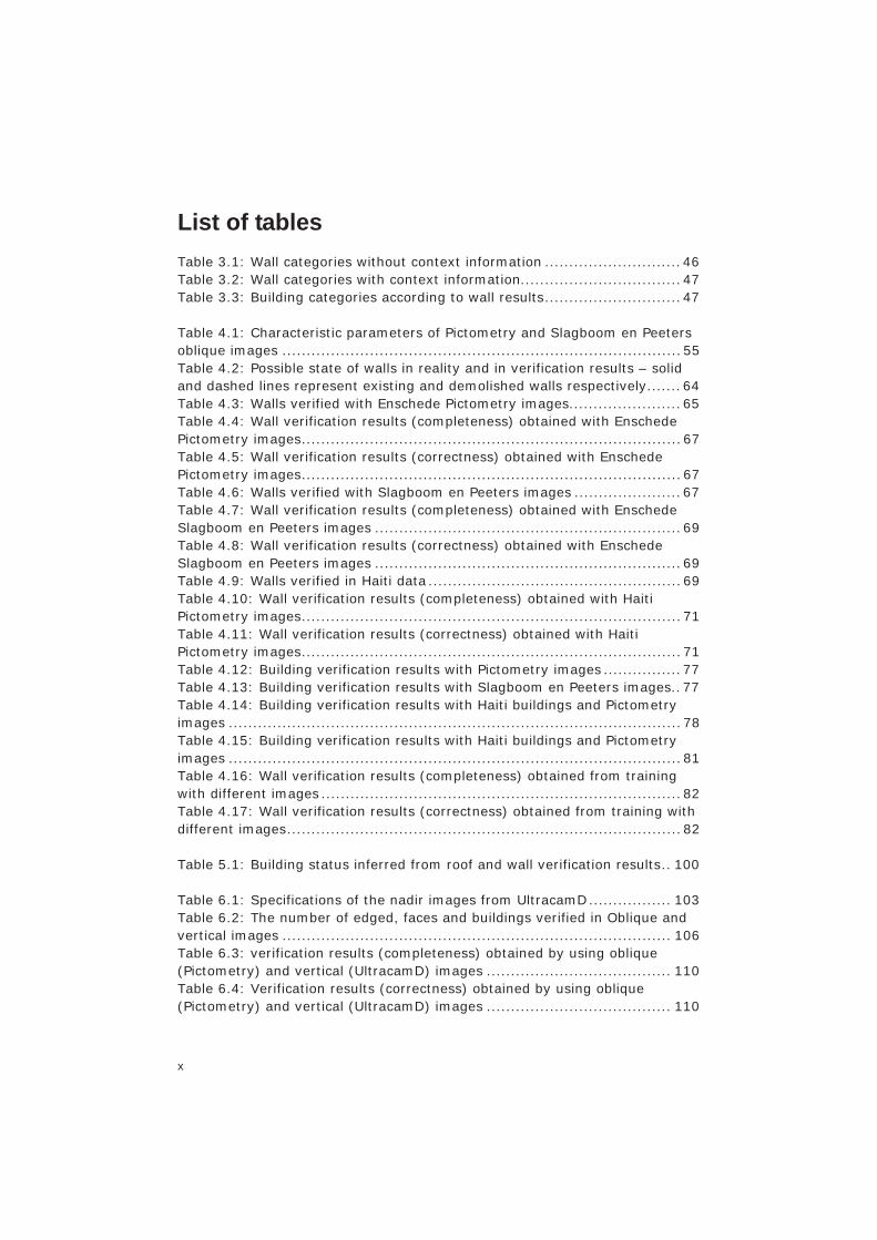
List of tables Table 3.1: Wall categories without context information ............................ 46 Table 3.2: Wall categories with context information ................................. 47 Table 3.3: Building categories according to wall results ............................ 47 Table 4.1: Characteristic parameters of Pictometry and Slagboom en Peeters oblique images .................................................................................. 55 Table 4.2: Possible state of walls in reality and in verification results – solid and dashed lines represent existing and demolished walls respectively ....... 64 Table 4.3: Walls verified with Enschede Pictometry images ....................... 65 Table 4.4: Wall verification results (completeness) obtained with Enschede Pictometry images .............................................................................. 67 Table 4.5: Wall verification results (correctness) obtained with Enschede Pictometry images .............................................................................. 67 Table 4.6: Walls verified with Slagboom en Peeters images ...................... 67 Table 4.7: Wall verification results (completeness) obtained with Enschede Slagboom en Peeters images ............................................................... 69 Table 4.8: Wall verification results (correctness) obtained with Enschede Slagboom en Peeters images ............................................................... 69 Table 4.9: Walls verified in Haiti data .................................................... 69 Table 4.10: Wall verification results (completeness) obtained with Haiti Pictometry images .............................................................................. 71 Table 4.11: Wall verification results (correctness) obtained with Haiti Pictometry images .............................................................................. 71 Table 4.12: Building verification results with Pictometry images ................ 77 Table 4.13: Building verification results with Slagboom en Peeters images .. 77 Table 4.14: Building verification results with Haiti buildings and Pictometry images ............................................................................................. 78 Table 4.15: Building verification results with Haiti buildings and Pictometry images ............................................................................................. 81 Table 4.16: Wall verification results (completeness) obtained from training with different images .......................................................................... 82 Table 4.17: Wall verification results (correctness) obtained from training with different images ................................................................................. 82 Table 5.1: Building status inferred from roof and wall verification results .. 100 Table 6.1: Specifications of the nadir images from UltracamD ................. 103 Table 6.2: The number of edged, faces and buildings verified in Oblique and vertical images ................................................................................ 106 Table 6.3: verification results (completeness) obtained by using oblique (Pictometry) and vertical (UltracamD) images ...................................... 110 Table 6.4: Verification results (correctness) obtained by using oblique (Pictometry) and vertical (UltracamD) images ...................................... 110

xi
Table 6.5: The number of edges, faces and buildings verified in Pictometry and Slagboom en Peeters .................................................................. 113 Table 6.6: verification results (completeness) obtained by using Pictometry and Slagboom en Peeters images ....................................................... 119 Table 6.7: Verification results (correctness) obtained by using Pictometry and Slagboom en Peeters images ............................................................. 120 Table 6.8: Combined wall and roof verification results ........................... 121

xii

1
1. Introduction
1.1 Motivation Topographic data is an important component in modern society as it serves many purposes including planning, taxation and location based services. The data is traditionally captured and maintained in databases of National Mapping and Cadastral Organisations (NMCAs). While objects, such as roads, property boundaries, water bodies and forests are equally important, we concentrate on buildings only. The data is mainly in two-dimensions (2D) where only the foot prints of buildings are maintained, but more and more three-dimensional (3D building model) data is also acquired. In this case, roof and wall structures of buildings are captured. Attribute information such as ownership or use type normally form part of building databases but we concentrate on the physical building structure. Topographic data acquisition for buildings is manual and time consuming but, for the 2D case, it has been completed for developed countries. However, there are usually changes which require continuous revision of the data. These changes may be, in some cases, obtained through planning processes because developments normally require planning consent before they are undertaken. However, this is not always done and even where it is done there are possibilities for errors due to construction not complying with approved plans. For developing countries, building databases are not complete and changes do not always follow planning procedures resulting in unplanned or squatter settlements. Verification and updating building databases and monitoring informal settlements (Ioannidis et al., 2009) by using means other than planning processes is therefore necessary. There are also changes that are not man made, such as building demolition due to disasters. These occur anywhere in the world, in developed or developing countries and for these cases, verification and update of existing databases using new data is required. Other than actual changes, building verification is required to identify cases where the data was wrongly captured. Both 2D and 3D data may contain errors, especially when they are captured by using automatic or semi-automatic methods. Checking and improving these datasets is therefore of importance. Revision is thus an important task for the usefulness of the building data. It involves using current raw data sources to check existing datasets for either of the following: a building in the database exists in the scene and complies to the database description; a building has changed or was captured with

Introduction
2
errors and has to be refined; a building is demolished or the data captured is wrong and has to be removed from the database; or a new building formerly not in the database is constructed and has to be captured. The actions involved are verification of existing objects, extraction of new ones, as well as refining geometry of the captured buildings. The main activities verify, detect change and update may be represented assets. Their containment is verify detect change update. Fig. 1.1 is an Euler diagram illustrating the subsets. Refinement is another term often used in relation to update. It implies activities for improvement of existing data (2D or 3D) such as improvement of geometric accuracy or addition of façade or roof details to existing 3D models.
Building Revision
Verify
Detectchange
Update
New captured (2D/ 3D)Extended to 3D
Improved geometry
New detected
Still thereDemolished
Changed
Building Revision
Verify
Detectchange
Update
New captured (2D/ 3D)Extended to 3D
Improved geometry
New detected
Still thereDemolished
Changed
Fig. 1.1: Processes involved in building revision - activities in verification are a subset
of change detection while both form part of update. Verification, change detection and update of building datasets have traditionally been done by manual inspection of aerial images. For datasets of whole cities or countries, this is not only labour and cost intensive but also time consuming. To reduce the burden, methods have been proposed for semi-automation and research for this purpose is ongoing. Some literature on methods proposed for this purpose include (Armenakis et al., 2010; Baltsavias, 2004; Haala and Kada, 2010; Heipke et al., 2004; Mayer, 2008). Issues include determination of the best data types to be used (such as stereo airborne or satellite images, ortho-photos or digital surface models). In general good results have been achieved but there are still many problems (cf. Section 2.1). For purpose of finding out what can be achieved in change detection of 2D building datasets, the European Spatial Data Research (EuroSDR) carried out experiments and compared results from different methods (Champion et al., 2008). From stereo images of a complicated urban scene at 20 cm GSD and a suburban scene at 50 cm GSD they derived and used CIR ortho-photos, a DSM and a DTM. A common aspect in all the methods tested is that buildings were identified by their height (using the DSM) and isolation from vegetation

Chapter 1
3
was by means of NDVI. Results showed problems in areas with poor quality of the DSM, particularly in shadow areas. The results indicate the need for more research. With ortho-photos and a DSM, only building heights and roof colour information relative to other objects was used. Information on side views of objects (e.g. walls of buildings) was not available. Images containing larger view of walls make buildings better recognisable. While roof colours are normally uniform because of the same type of roofing materials, wall façade have texture and pattern (such as horizontal and vertical lines) that make a building better identifiable. A building may be identified better when both roof and wall clues are combined. Traditionally, acquisition of building information has been done using vertical images with side and forward overlap to allow stereo processing. Today there are new sources that may be exploited for better results. In multiple overlapping vertical images from Intergraph DMC or Vexcel Ultracam (Gruber, 2007; Petrie and Walker, 2007) a scene is seen in many images. The redundancy can be used to better identify features in the scene. More recently oblique images are systematically acquired in addition to vertical images. These images capture a scene from different sides. Examples are Pictometry and MIDAS systems which capture 5 images at every point; one for each north, south, west, east and nadir (Petrie, 2009). Pictometry data is available for cities of Europe with over 50,000 inhabitants (Lemmens and Lemmen, 2007; Wang et al., 2008b). The data is used mainly for visualisation purposes such as in Microsoft Bing Maps. With the current imaging technologies, multiple oblique images are acquired without much cost in addition to the capture of nadir looking images. At the same time, the oblique images have a lot of potential not only for visualisation but also for verification and updating of existing building datasets. Vertical images have a limited view on walls of buildings while both roofs and walls are imaged clearly in oblique images. The acquisition of images with the presence of walls of buildings throughout the imaged area at an angle of at least 200 requires vertical images with a very high overlap (Meixner and Leberl, 2010). Besides, the availability of all sides of buildings will require cross flight patterns or very high side overlap. Although with oblique images there is more occlusion and we cannot see all sides of a building in one image, the combination of images from different perspectives gives a lot of information in addition to what we get from vertical images alone. In Fig. 1.2 oblique views of the same scene are overlaid with the 2D large scale topographic data (GBKN). Notice the correct fit of the outlines in the images for building sides facing the camera. Roofs and walls in these images are recognisable. Information on a complete

Introduction
4
building may be exploited for better automatic verification, change detection, and update of building map information.
Fig. 1.2: Different oblique views of buildings overlaid with a 2D GIS data. The overlay
is visually accurate. Images © Blom
1.2 Research objectives Verification, change detection and update of building datasets is normally done by using airborne vertical images or airborne lidar. Proposed solutions are not yet mature and the processes are mainly based on height and colour of roof hypotheses (cf. Section 1.1 and 2.1). Roof as well as wall faces of buildings are better portrayed in oblique images but oblique images are not normally used for acquisition and update. Reasons why oblique images are rarely used include unavailability (in the past), scale variations within the image and occlusion. While standard image acquisitions are only twofold overlap for stereo processing, views of all sides of a building require multiple perspective images. Although a combination of vertical airborne images and terrestrial images can also be used for obtaining roof and wall information, this is not an optimal solution: acquisition of both airborne and terrestrial images is more costly than airborne oblique images taken from different directions. Besides, with mobile vehicles, terrestrial images will contain only walls that are facing streets. Currently, there are operational systems (discussed in Section 2.2.2), for acquisition of vertical and oblique images without much additional cost compared to vertical image acquisition only.
Chapter 1
5
Datasets collected regularly and systematically are also available but have not yet been used for automatic verification and update of buildings. The objective of this work was to develop a method for automatic verification of building vector data in existing databases using airborne oblique images. Specific objectives are: 1. To verify building information in 2D (large scale topographic dataset). To
use oblique images to determine whether a building in the database exists in the scene (the data is correct), was changed (or wrongly captured) or was demolished.
2. To verify building information in 3D (3D building models). To use oblique
images to determine whether a building exists in the scene (the data is correct), was changed (or wrongly captured) or was demolished.
In order to meet these objectives, the following questions are answered in this research. 1. How can we use oblique images to verify 2D building outlines?
1) How can the area containing a building be identified in an oblique image given only a 2D outline and the problem of (self-) occlusion?
2) What are the suitable features for building verification using oblique images and which role do the individual facades play in this context?
3) How can features be extracted in single images and how can they be combined to define a reasonable verification measure per wall?
4) How can different measures for verification of a wall in oblique images be combined to an overall measure for the wall and how can uncertainty be considered?
5) How can wall verification measures be combined for a building verification?
2. How can we use oblique images to verify 3D building outlines?
1) How can images containing a building be identified given a 3D building model and the problem of (self-) occlusion?
2) What are the suitable features for 3D building model verification using oblique images?
3) How can uncertainty in the image and models be considered? 4) How can evidence be combined for a model face and the whole
building? This work does not cover change detection and update tasks required for complete building revision. For more details on scope and assumptions are in Section 1.4.

Introduction
6
1.3 Innovation in this work This research investigated the usefulness of oblique airborne images for automatic verification and update of building datasets. Two methods were developed, the first for verification of building outlines in a large scale topographic database (2D) and the second for verification of 3D building models. In both methods, the vector data was fitted to multiple oblique images and features derived from the images were used to do the verification. The innovation in this work is: Firstly, the method developed for verification of 2D building outlines uses airborne oblique images, a data type that has mainly been used for visualisation but not often used for vector data acquisition, verification or update. Secondly, while methods suggested in other research works utilise roof information such as roof colour or building heights relative to the ground, the method developed in this work verifies 2D building outlines by using wall information. Thirdly, the method developed for verification of 2D building outlines starts by verifying individual walls of a building and then the results are combined for overall verification of the building. Because of this approach, buildings that may have changed by part demolition or extension are signalled when only some walls of a building are identified in the images. A number of features suitable for recognising a wall in oblique images were therefore developed and strategies to combine these features in an overall measure of the status of a wall and a building were designed. Lastly, the theory of mutual information was adopted to obtain an automatic method for verification of the 3D building models. The method developed assumes that the pixel gradient directions computed along a model edge should be generally different from gradient directions computed on random image positions. These gradient directions were found to be very robust for verification.
1.4 The scope and assumptions Although detection of new buildings is important for complete updating of existing datasets, the scope of this work was on verification of existing datasets only. A different project for detection of buildings in oblique airborne is underway and preliminary results were reported (Xiao et al., 2012). In the developed method the following are assumed. Firstly, it is assumed that vector datasets (buildings in 2D) are available and that they are of large
Chapter 1
7
scale and not further generalised. For 3D building models we assume CityGML (Kolbe et al., 2005) level of detail 2 or 3 for the roofs. Secondly, it is also assumed that oblique images are available and with these characteristics: large scale corresponding to the pixel ground sampling distance (GSD) of less than 20 cm to provide roof and wall façade details, taken from different directions to provide all sides of imaged buildings and with overlap. Lastly, the camera interior and exterior orientation information for the images is assumed to be available.
1.5 Thesis outline The second chapter presents the state of art building verification and update and the current use of oblique images. The third chapter describes the method developed for automatic verification of 2D vector data (building outlines). Chapter four discusses experiments and results from the verification of building outlines. Chapter five presents the method developed for verification of 3D vector data (3D building models). Chapter six presents 3D building verification experiments. The last chapter contains conclusion and recommendations. Some parts of this thesis are based on papers published during the research (Nyaruhuma, 2010; Nyaruhuma et al., 2010a; Nyaruhuma et al., 2010b; Nyaruhuma et al., 2012a; Nyaruhuma et al., 2012b).

8
2. State of the art Before going to the methods developed in this research this chapter is dedicated to a discussion of what has been done in other researches. The discussion is on two aspects related to building verification. In the first place it is a review of the methods and data used and the results that can be achieved and in the second place the discussion is on the current use of oblique images.
2.1 State-of-the-art building verification Building verification is often combined with detection of new buildings (together referred to as change detection, see Section 1.1). Methods discussed in this section are therefore not necessarily proposed solely for verification. Features that are derived from data are used not only for the purpose of providing evidence for correctness of buildings available in a database but also for suggesting the presence of new ones. Although today there are technologies for acquisition of different data types such as airborne laser scanning point clouds, radar or airborne hyper-spectral images, we concentrate on airborne images and digital surface models (DSM) from image matching or airborne laser data. The discussion is divided into two main parts: one for verification of 2D data (building outlines) and another for verification of 3D data (3D building models). Other objects of interest for automatic verification in the urban context are roads but they are not covered in this research. We only note here that, through overlay and comparison of oblique image segments to an existing road dataset, inconsistencies could be detected (Mishra et al., 2008). Readers interested in verification of roads may also refer to (Agouris et al., 2001; Gerke and Heipke, 2008; Zhang, 2004).
2.1.1 Verification of 2D building outlines Many methods proposed for verification of building outlines use 2D clues (e.g. colour or line features in ortho-images) but buildings are generally higher than their surrounding ground. Methods have therefore evolved for verification of 2D outlines taking 3D features into consideration (e.g. building height in a DSM). In literature, the main approach to 2D building verification using 2D clues is classification of images and comparison of the results to existing datasets. The data used is either airborne or high resolution satellite images. Verification of 2D building outlines using airborne images: In (Olsen et al., 2002) a typical classification procedure for change detection was carried out using the colour of objects. The data used was CIR and RGB

Chapter 2
9
and the classification was supervised considering the colour of roof of some existing buildings. The results were compared with a raster map. For a sub-urban test area with 61 simple buildings, all buildings were detected using CIR and RGB but roads were also classified as buildings because the colour of asphalt was one of roof colours in the training dataset. Five buildings removed from the dataset to simulate new buildings were identified in CIR while 2 were missed by RGB. Verification of 2D building outlines using satellite images: A number of research works involving high resolution images already exists. A sample of these works is described here. Firstly, using the German topographic database (ATKIS), classification of object using high resolution satellite images was done (Walter, 2004; Walter and Fritsch, 2000). The intention was to differentiate areas in the images as water, forest, settlement, and greenland for purpose of updating the existing database. The approach was 2D classification using existing GIS data as knowledge. The intended detection and update was for a topographic dataset at the scale of 1:25,000, geometry accuracy of 3m. Due to the resolution and only 2D hypothesis used, 9% of the objects existing in the database were assigned in wrong classes from the image. The second work using the high resolution images from Ikonos and Quickbird is by Bouziani et al. (2010; 2007). Segmentation was done using existing knowledge (considering NDVI, shadows and compactness). They also used a combination of change detection rules (spectral - comparing with existing knowledge, geometric - buildings should be compact, and transition - new buildings in bare soil or vegetation). The databases for update were of scale 1:10,000 and 1:20,000 but 20% of buildings could not be detected and geometric errors reached 5 meters between detected building and those existing in the databases. The low accuracy was due to similarity of colour of building to non building areas and the low spatial resolution of the images. A third sample of studies involving high resolution satellite imagery is by the Ordnance Survey of the United Kingdom (Holland et al., 2006; Holland and Marshall, 2004). Their interest was not on automation but to find out what can be achieved by using experienced surveyors and cartographers in testing usability of the images for manual photogrammetric extraction and verification of existing objects. Objects were captured by using ortho-rectified Quick-Bird panchromatic images. It was generally concluded that the images are useful only for small scale mapping at scale of 1:10,000 or lower. Another conclusion was that the images may be useful for manual verification but other datasets or field visits would be required for update. The reason for this conclusion is that buildings could be detected in the images but the geometry of the boundaries could only be generalised to rectangles.
State of the art
10
Recent research on building verification using high resolution satellite images have also shown that there are too many errors for the data to be useful operationally (Champion et al., 2010; Ehlers et al., 2010; Le Bris and Chehata, 2011). The problems include dark building roofs which are misclassified as roads and red roof tiles which are classified as bare earth. Other reasons include difficulty of differentiating single storey buildings from the bare ground by using coarse DSMs derived from the images. Verification of 2D building outlines using digital surface models: A DSM is another data type used for detecting changes in building information. The DSM is obtained from airborne laser or by dense matching of aerial images. For change detection using a DSM there are two possibilities, to compare two DSM datasets obtained at different times (Alobeid et al., 2011; Vögtle and Steinle, 2004) or to compare a new DSM with an existing map. The former is interesting because height differences in the datasets can be compared. In practice, however, old data is usually not available; instead the new data is compared to buildings in existing databases. Olsen (2004) derived a coarse DSM from stereo images and used it to derive height information for building change detection. Using images, areas were pre-classified using pixel colour. During this step, NDVI was used to identify vegetation. The final decision was done taking into account the main idea that buildings are higher than the ground. With a test set containing 14 demolished and 12 new buildings, 2 demolished buildings were not identified, 10 new buildings were not identified and there were 45 false new buildings. The main reason given was uncommon roof colour and buildings covered with trees. Vosselman et al. (2004) used a DSM, for segmentation and classification into bare ground, buildings and trees. Building segments were compared with buildings in existing topographic map to detect buildings that are new, changed in size or shape, or demolished. Because buildings are captured with special rules defining which buildings are allowed in the database, the change detection procedure made use of the same rules in the mapping catalogue. The intended scale was 1:10000, thus generalization inherent in the existing data was faced. In the results, 15% of building points were classified as vegetation and 22% of vegetation points were classified as building points. The main reasons for the misclassification were generalisation of the buildings, the mapping rules used in the acquisition of the buildings and the point density where some building segments had very few points and were misclassified as trees.

Chapter 2
11
Research for automation of 2D building verification using DSM is also described in Champion (2007), Matikainen et al. (2007) and Rottensteiner (2007). The methods of the three authors were tested using a reference dataset manually prepared (Champion et al., 2008). The test included verification of existing buildings and detection of new ones. They used high resolution images and a DSM derived from the images. Most buildings in the database were correctly verified (completeness of 80% to 98%) but there were also many false alarms (correctness of 45% to 58%). The reasons for the alarms were shadows which affected the quality of the DSM. Even with a better DSM some errors would probably still be present because the height information sometimes leads to detecting vegetation as buildings. In general, the information used for verification of 2D building outlines is either roof colour or height relative to other objects in the scene. However, a research (Zebedin et al., 2006b) using Vexcel Ultracam vertical images, where side views are available especially in border areas, demonstrated a potential inside view information available in airborne images. Despite a limited side view in vertical images – when compared to oblique images - façade lines detected in the images were useful to ascertain the proper position of walls.
2.1.2 Verification of 3D building models Some methods have been proposed for 3D building model verification. Huertas and Nevatia (2000) projected 3D models to images for detecting changes in the 3D models using monocular aerial images. They used evidence such as edges and shadows to hypothesise and verify walls from images. Because the images used were vertical, walls were not depicted well and information from one image could not be confirmed in another image because only one image was available for a scene. Suveg and Vosselman (2004) used vertical images (stereo pairs) for verification of 3D models. Their method was not used for identifying existing and demolished buildings because their main intention was to model buildings given footprints and images. Therefore, several possible roof geometries were generated and the verification was done for selecting a predefined model which best fits the images. Another 3D model verification procedure (Knudsen, 2007) uses supervised classification in airborne images. The procedure is similar to comparison of 2D datasets to segmented ortho-images but in this case 3D information for individual roof faces was available for projection to the images using orientation information. They segmented the images and categorised segments as building areas by comparing them to a training dataset. The dataset for verification contained buildings built apart from each other, with

State of the art
12
simple roofs and similar roofing materials. With a small test sample, 6 out 102 existing buildings were not detected and one demolished building was not identified. The main cause for wrongly categorised buildings was roof colours that were not present in the training dataset. There are also methods in literature where multiple images were used for verification of buildings. The images used are either taken at the same time or multi-temporal. Using images taken at the same time, building verification is done by utilising object indifference in multi-perspective images. In the case of multi-temporal images verification is done by comparing old images to new images expected to contain changes. Taneja et al (2011) utilised multi-view images for detecting changes in buildings represented in 3D models. They explored texture invariance of building faces in multi-view terrestrial images. In their approach true positive changes increase with increase in false positive changes. They reported that 90% true positive changes coincided with 10% false positive changes. The main problem for general usability of terrestrial images captured by mobile vehicles is that only the sides of buildings facing streets can be analysed. The rear sides of buildings and backyards may not be imaged and changes such as extensions to buildings in these sides may therefore not be identified. In (Boudet et al., 2006), the images were of overlapping airborne vertical type. The clues used included the comparison of lines, corners and colour of image patches. The problems reported include the cases where some edges of a face were correct and other incorrect but because the decision was per face the overall result was a wrong average. There were also many incorrect faces that were categorised as correct (20% of faces accepted as correct) when they were correct in 2D location but wrong in height. This happened because objects at the same 2D position are located in nearly the same area when captured in vertical image. Another method was also proposed for using oblique images to verify buildings in existing datasets (Nakagawa and Shibasaki, 2008). The method requires three accurate datasets: firstly, an old 3D building model with all the buildings to be verified, secondly old high resolution oblique images containing all the buildings in the model and thirdly new oblique images representing the current situation. The strategy used is projecting the old 3D models into both old and new oblique images to obtain image patches of the model faces in both images and then compare the patches using cross correlation. Experiments were done for a set with 767 correct model faces and by using images taken with the Three Line Sensor (Gruen and Zhang, 2003). In the first round of experiments 84% correct faces were confirmed. The remaining faces were not identified due to differences in shadows in the

Chapter 2
13
images taken at different times. In an improved method a procedure to identify and avoid areas with shadows was developed. Then they recognised 90-100% faces by using cross correlation and histogram subtraction methods. Only 2 incorrect faces were tested and were identified.
2.1.3 Discussion Building verification is difficult to automate particularly for complex urban environments with buildings of different types and heights. Existing methods especially for 2D building verification and update use the facts that colours of roof faces are similar and may be differentiated from the rest of imaged objects and that buildings are elevated compared to the surrounding ground. The methods that utilize roof colour and height information for building verification sometimes give wrong results. When using the difference of the height and the colour between roofs of buildings and the surroundings of the buildings, the variation is sometimes not strong enough and a building may be confused for other objects such as the ground or vegetation. Side views of buildings might be of additional help in this context because the vertical structures are then visible directly and not only implicitly through derived height information. A hypothesis concerning a different appearance of facades compared to the surroundings can be formulated as well and is much stronger than only roof information. Objects on the whole structure of a building, on walls as well as on roofs, can be clearly seen in oblique images because of the tilted view. Similarly, building height changes should be better identified in oblique images than in vertical images. Thus, methods developed in this research utilize building information available in oblique images.
2.2 The current use of oblique images Research on utilisation of oblique images has gained interest in recent years. Unlike vertical images where mainly top view structures (roofs - for buildings) are seen, in oblique images we also see sides of objects (walls –for buildings). Oblique images are therefore appealing to humans and buildings can be better recognised than in vertical images. Oblique images, however, have traditionally been neglected as a data input for photogrammetric work due to their characteristics. This part discusses the characteristics of oblique images, followed by recent development in their acquisition, processing and use. The reasons for this introduction are on one hand to identify characteristics of oblique images which we can take advantage of (or be constrained by) in automatic object recognition and to reflect on the relative recent easy of acquisition. On the other hand the introduction intends to
State of the art
14
identify demerits of oblique images which building verification methods developed have to take into account.
2.2.1 Characteristics of oblique airborne images Unlike vertical images, which are taken at a small tilt encountered due to the movement of the platform, oblique images are purposely taken at a relatively large angle. While vertical images are normally captured at a maximum tilt of 5 degrees, oblique angles are as big as 30 to 50 degrees. Basic characteristics of oblique images are discussed in photogrammetric textbooks such as the Manual of Photogrammetry (McClone et al., 2004) but also research works such as (Höhle, 2008). The characteristics include higher variation of scale from the foreground to the background. Because of their nature, the use of oblique images has usually been limited to special cases such as in the military, in the areas not easily reachable or in monitoring of progress of construction projects (Slama et al., 1980). The flying height above terrain and focal length are important for determination of scale, in the same way as in vertical images but for oblique images, scale at a point in the image is related to two other parameters. These are the tilt of the camera from the vertical and the angle between the line from the point to the lens of camera and the vertical. This relationship is shown in Fig. 2.1. In that figure a constant terrain height is assumed.

Chapter 2
15
B’
h
O
back B P front
f
O - perspective centreP - principal point projected to terrain planeP’ - principle point in imageB - measured objectB’ - measured object in imagef - focal lengthh - flying height
- half field of view- angle between viewing direction of B and the vertical- tilt of the camera
P’B’
h
O
back B P front
f
O - perspective centreP - principal point projected to terrain planeP’ - principle point in imageB - measured objectB’ - measured object in imagef - focal lengthh - flying height
- half field of view- angle between viewing direction of B and the vertical- tilt of the camera
P’
Fig. 2.1: The geometry in oblique images
The scale of an oblique image varies. At any object point B in the image, the scale S is given by:
)cos(.cos.
hfS
where . (1) Because the flying height, the tilt of the camera and the focal length are fixed
for a given oblique image, the respective variables fh ,, in the scale equation are constant. Then the scale varies but only depending on the
position of an object in the image defined by the angle between the viewing direction of the object point and the vertical direction. If the object point B is at the foreground, background or at a ground point
corresponding to the principle point in image, then in the equation is equal to , or respectively. Another characteristic of oblique images is a higher effect of occlusion. In Fig. 2.2 a tower building captured in two oblique images and one vertical image is presented. In the oblique image (middle) we can not see the small building

State of the art
16
behind the tower while in the vertical image (right) the roof of the small building can be partly seen. In addition to roofs, in oblique images interest is also to walls. To analyse all sides of a building images from different sides are required.
Fig. 2.2: Building occlusion in oblique images - the small building in the left image is completely hidden in the oblique (middle) image but it is partly visible in the vertical
(right) image. Images © Blom The other characteristic of oblique image is that instead of only top view that we see in orthogonal images (Fig. 2.3 left) we can see the whole vertical structure of a feature (Fig. 2.3 right), given it is not occluded by other object in the foreground. The same building gives different impressions to a viewer. The oblique view is more appealing and contains more details.
Fig. 2.3: Orthogonal and oblique views of a building - in the oblique image we see, in addition to the roof, walls and their features such as wall edges, windows and doors.
Images © Blom
2.2.2 Acquisition of oblique images In recent years, interest and studies for use of oblique images have increased. The reasons are not only because objects in oblique images can be easily interpreted by humans but also there is an increase in development of sensors and platforms for their acquisition. An overview of the trend in

Chapter 2
17
imaging technology was written by Petrie and Walker (2007). Images can also be acquired with relatively cheaper platforms such as unmanned aerial vehicles (UAVs). Sensor systems for airborne image acquisition have evolved from traditional capture of vertical images where along track overlap is used for stereo analysis to different types of systems for acquisition of oblique images in addition to vertical ones. Although mid-frame cameras have also been used for multi-view oblique image acquisition recently (IGI, 2013a), cameras mostly used are non-metric. The non-metric cameras are less expensive and several of them can be carried on the platform. The increased quality of small-frame semi-professional cameras has generally pushed forward the acquisition of multi-view images. A comprehensive overview on operational systems for acquisition of oblique airborne images was published by Petrie (2009). Some systems capture one vertical and one oblique image, at one point, such as forward view or side view. Examples are FLI-MAP of Fugro Aerial Mapping B.V. (2011) for vertical and forward, and PFIFF camera system by (Grenzdörffer et al., 2008) for side views. Other systems capture two oblique images in addition to vertical ones where the oblique images are either captured along track with front and back view or side looking left and right. Three Line Scanner (TLS) is an example of three image capture system with along track views (Gruen and Zhang, 2003). TLS oblique images are taken at small angle (21o). Side views are better than vertical images but still limited compared to oblique images taken at a larger angle. The German Aerospace Center (DLR) has developed the 3K camera system for vertical and side views at a larger angle such as 31o (Kurz et al., 2007a; Kurz et al., 2007b). More recently, systems have been developed for capturing five images at the same time (Petrie, 2009). The images captured are, one at nadir (vertical image), two at opposite directions cross–track and the other two in opposite directions along-track. Considering forward and side overlap, a scene is therefore captured in multiple overlapping images. Examples include systems used by Pictometry and their licensees such as Blom (Wang et al., 2008b), MIDAS (2011) and Slagboom en Peeters Luchtfotografie B.V. (2011). Since the companies currently do not focus on accurate direct sensor orientation, because they are focusing on visualization applications, some additional effort to compute accurate sensor orientation is necessary (Gerke, 2011).

State of the art
18
2.2.3 Current utilisation of oblique images Mono-plotting: Plotting a feature in a single image requires some height information of the imaged place. The system of Pictometry called Electronic Field Study (EFS) uses an existing digital terrain model (DTM) for making 3D measurements in oblique images. Using the EFS software, measurements have been made and the results are in the range of errors of 2 meter in planimetry and 0.5 meter in height (Höhle, 2008). The accuracy of the measurements depends on the quality of the DTM and of image orientation and calibration parameters. Visualisation: Oblique images have been used mainly for visualisation including bird’s view in virtual worlds such as Microsoft Bing Maps. 3D Modelling and texturing: More recently the acquisition of multiple overlapping images, vertical and oblique, has triggered research in their use. Even with limited façade information, some studies have proposed building model texturing using wall features that can be observed in the edges of orthogonal images acquired using wide angle cameras (Zebedin et al., 2006b). Instead of orthogonal images, Grenzdörffer et al. (2008) used the MultiView system for extraction of façade and for texturing of 3D building models using multiple overlapping oblique images. Also in other studies oblique images have been used for texturing 3D models (Frueh et al., 2004; Wang et al., 2008a). Building modelling and update: For cadastral purposes existing data was overlaid on Pictometry oblique image (Lemmen et al., 2007). It was concluded that oblique images are interesting as a source of information for real estate management and taxation. Multiple overlaps of the images or their use for updating building information was not done. Image Matching: It has also been shown that images matching using oblique images gives good results (Furukawa and Ponce, 2010; Gerke, 2009; Haala, 2011; Le Besnerais et al., 2008). Automatic object recognition and change detection: For verification of road data in existing dataset a study was conducted (Mishra et al., 2008). They classified an oblique image, overlaid the result with vector data (roads) and analysed overlapping areas. They could detect inconsistencies between the roads as in the image and as in the dataset. They did not verify buildings except for cases such as new buildings on or occluding a road.

Chapter 2
19
Another classification procedure was done for the purpose of assessing structural damage caused by earthquake (Gerke and Kerle, 2011). The intention was to assign every building to either of categories no-moderate damage, heavy damage and destruction. Despite the overall accuracy of only 63% - which was also partly caused by the fuzzy definition of building damage - they reported potential in using oblique images. The literature we could obtain on building verification using oblique images was only by Nakagawa (2008). As introduced in Section 2.1.2, they used multi-temporal oblique images to verify 3D building models and reported good results. Although tests with incorrect faces were limited, their texture comparison approach is interesting and a similar approach was reused in obtaining one type of verification measures developed in this work (cf. Section 3.3.4). In our case the data verified is 2D building outlines and in place of multi-temporal we have multi-view images.
2.2.4 Conclusion In this chapter we have discussed previous research on automatic verification of building datasets. In most cases the data used for verification purpose is vertical images. We have also discussed interesting characteristics of oblique images that may be utilized for better verification of buildings. Airborne oblique images have advantages over vertical images in that buildings can be identified in oblique images by using information on the roofs as well as walls. Today there are new developments where many images of the same scene are taken from different directions. We can take advantage of views of different sides of buildings where features occluded in one image may be visible in another and at the same time some sides can be visible in multiple overlaps. Oblique images, however, are not commonly used for automatic detection of buildings due to their characteristics including occlusion and different geometry. There are also challenges in combining multiple images in order to obtain information of the whole structure of imaged features. Research for automatic detection and verification of buildings in oblique images is still scanty. In this research, oblique images are used to derive information about the whole structure of a building, roofs and walls. A building in the vector data in 2D (building outline) or 3D (building model) earlier captured are examined for either of the following: whether data for the building was captured correctly and the building has not been changed; the data was wrongly captured or the building has been demolished or; the data is partly correct or the building has been modified.

State of the art
20

21
3. Verification of 2D building outlines using oblique airborne images1
Topographic dataset datasets of buildings were traditionally captured in two dimensions where only building footprints are acquired and the position and size in vertical direction is not considered. Although in recent years more and more 3D building models are acquired, most datasets are still in 2D. Therefore, methods for verification of buildings are required both for the 2D outlines and 3D building models. For the 2D case, there are already methods proposed for verification by using 2D clues but there are problems, c.f. Section 2.1.1. This chapter presents a method developed for automatic verification of building outlines in 2D large scale topographic datasets. The verification is done by using clues on walls in oblique images. Oblique images required are those taken at angles large enough to allow recognition of details on wall façades. While the façade information available in oblique images may be interesting for identifying the number of floors or usage of a building such as industrial or apartments, in this work concentration is on identifying whether the building represented in vector data still exists (correct data), has been demolished or is changed. The verification approach is introduced in Section 3.1 and followed by the description of visibility analysis, the procedure for identifying parts of the buildings that may be occluded by other buildings or vegetation (Section 3.2). In the developed method several clues are converted to measures of existence of a wall. How each of the measures is derived and used for obtaining a certain level of acceptance that a wall exists is described in Section 3.3. In Section 3.4, methods for combining evidence from different clues are discussed. Section 3.5 describes the use of additional evidence for a wall given results of adjoining walls and Section 3.6 is for the final decision on building status. Experiments are discussed in Chapter 4.
3.1 The approach In chapter 2.1.1 research works that use vertical images to exploit roof characteristics for building verification were discussed. The main problems include mixing of roof with non-roof objects due to similar radiometry and 2.5D height information that might not always be strong enough. Wall information is limited in vertical images and was not used in those works. In this work, verification of building outlines is based on clues on walls in
1 This chapter includes contents from Nyaruhuma (2010), Nyaruhuma et al. (2010a), Nyaruhuma et al. (2010b) and Nyaruhuma et al. (2012).

Verification of 2D building outlines using oblique airborne images
22
oblique images. The main contribution is exploiting building wall information. Thus, evidence from the roof is not used directly in this research. This section briefly describes our definition of building verification and the assumptions taken into account. It also briefly introduces the main processes and the preliminary step of generating wall hypotheses.
3.1.1 The building verification model Verification is observing an object for establishing whether or not it conforms to specified standards. For our purpose, building verification is to find out if the large scale topographic vector data representing a building fits the actual ground situation. A segment of a building outline representing a wall of a building is verified as existing or correct if there is evidence of a wall at the location defined by the segment and a small tolerance. On the other hand, the segment is not correct or the wall is demolished if it cannot be justified. A building is verified according to the state of its walls. If all walls of a building are correct the building is verified as unchanged. Alternatively, if all walls are identified as demolished, then the whole building is categorised as demolished. If only some walls of a building are correct, then the building is modified either by extension or part demolition.
3.1.2 Assumptions in building verification In this work, it is assumed that walls may be recognised in airborne oblique images. When a building is partly occluded by other buildings or trees evidence from wall faces which are visible in the same or other images are used to make the overall assessment of the building. At least one façade should be visible for this method. Because images used to verify a building are taken during the same flight, we assume a static scene in regard to the buildings. It is also assumed that wall faces are planar and vertical. Because in this case the building data being verified is in 2D, a wall is represented by a line segment joining two nodes of a closed building footprint (polygon). Moreover, the ground elevation as well as the position and geometry of roofs are undefined. For this reason an estimate of the ground elevation is required for approximate location of walls and if at least a coarse DSM is available then it may be used to derive heights of the wall hypothesis.

Chapter 3
23
A building outline to be verified and one of the images in which the building is visible are shown in Fig. 3.1. For the images, it is assumed that the camera’s interior and exterior orientation information is available.
Fig. 3.1: The footprint of building to be verified (left) and the same building in an
oblique image ©Blom
3.1.3 The verification process In the developed method, each building is verified by combining evidence from individual walls. The main components of the method are indicated in the flow chart shown in Fig. 3.2. Several clues on the existence of a wall in an image are used: Wall façade edges extracted from images taken from different
perspectives are expected to coincide when projected to the respective wall plane in object space.
The directions of most façade edges are expected to be horizontal or vertical in object space.
Outer building edges are expected to coincide with corresponding lines extracted in images.
The textures of patches of images of the same wall taken from different viewing directions are expected to be highly correlated.
These clues are converted to a measure of existence of a wall. Each measure is a numerical value obtained by projecting images to the vertical wall being verified. The measures are described in Section 3.3 below. Verification measures are combined for each wall in order to obtain the overall wall result. For this purpose we adopt and compare three reasoning approaches, namely the Hint theory (Hints), Adaptive boosting (AdaBoost) and Random trees (RTrees). In the first approach, training samples are used

Verification of 2D building outlines using oblique airborne images
24
to draw scatter plots and manually construct fuzzy membership functions for each of the measure. In this case, subsequent verification of walls is done by combining evidence from these functions. The combination is done using the theory of Hints (Kohlas and Monney, 1995) which is derived from the Dempster Shafer Theory of Evidence (Dempster, 1967; Shafer, 1976). Further, the training samples are used for training AdaBoost (Freund and Schapire, 1997) and RTrees (Breiman, 2001). Once each wall has been categorised as existing or demolished the status of the whole building is decided. A building is categorised as unchanged, demolished or modified.

Chapter 3
25
Fig. 3.2: Flow char of the main processes in the building verification approach
3.1.4 Definition of wall hypothesis In order to obtain wall evidence in oblique images the first step is to make the hypothesis on the position of the wall in the images. This procedure is introduced here. Visibility analysis, derivation of verification measures, and their combination will be discussed in following sections.
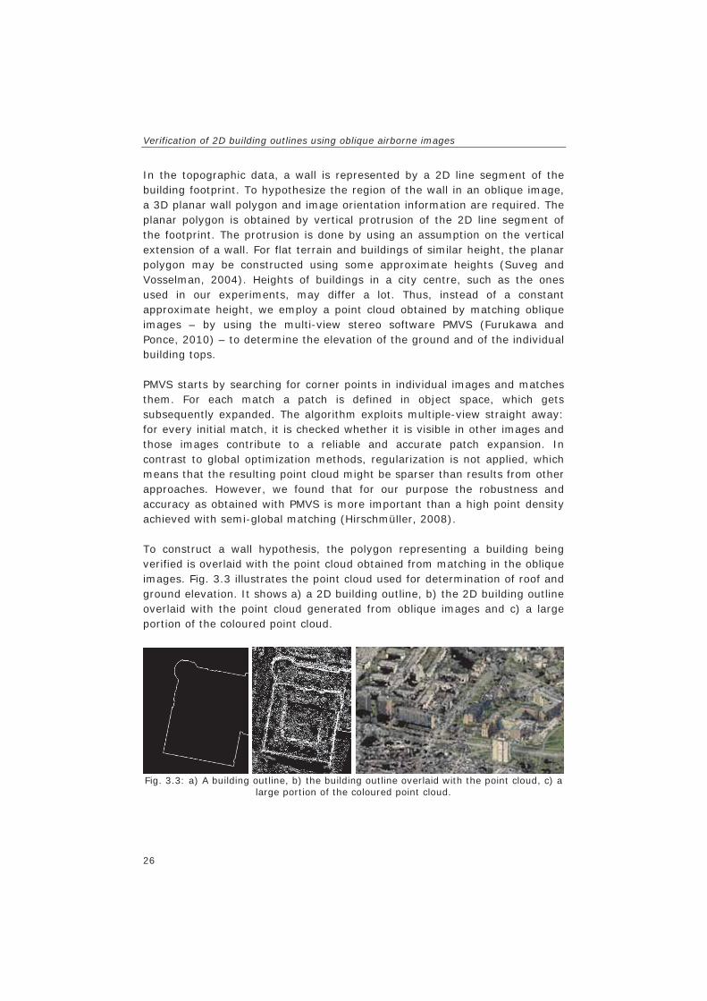
Verification of 2D building outlines using oblique airborne images
26
In the topographic data, a wall is represented by a 2D line segment of the building footprint. To hypothesize the region of the wall in an oblique image, a 3D planar wall polygon and image orientation information are required. The planar polygon is obtained by vertical protrusion of the 2D line segment of the footprint. The protrusion is done by using an assumption on the vertical extension of a wall. For flat terrain and buildings of similar height, the planar polygon may be constructed using some approximate heights (Suveg and Vosselman, 2004). Heights of buildings in a city centre, such as the ones used in our experiments, may differ a lot. Thus, instead of a constant approximate height, we employ a point cloud obtained by matching oblique images – by using the multi-view stereo software PMVS (Furukawa and Ponce, 2010) – to determine the elevation of the ground and of the individual building tops. PMVS starts by searching for corner points in individual images and matches them. For each match a patch is defined in object space, which gets subsequently expanded. The algorithm exploits multiple-view straight away: for every initial match, it is checked whether it is visible in other images and those images contribute to a reliable and accurate patch expansion. In contrast to global optimization methods, regularization is not applied, which means that the resulting point cloud might be sparser than results from other approaches. However, we found that for our purpose the robustness and accuracy as obtained with PMVS is more important than a high point density achieved with semi-global matching (Hirschmüller, 2008). To construct a wall hypothesis, the polygon representing a building being verified is overlaid with the point cloud obtained from matching in the oblique images. Fig. 3.3 illustrates the point cloud used for determination of roof and ground elevation. It shows a) a 2D building outline, b) the 2D building outline overlaid with the point cloud generated from oblique images and c) a large portion of the coloured point cloud.
Fig. 3.3: a) A building outline, b) the building outline overlaid with the point cloud, c) a
large portion of the coloured point cloud.

Chapter 3
27
Ground and wall elevations are approximated by using the heights of the cloud points and taking into consideration the possibility of non-ground and non-roof points due to chimneys or noise in the data. The individual points in the vicinity of a particular building to be verified are first selected using a buffer around the building polygon. The noise points are expected not to belong to big continuous segments of roofs, walls, trees or ground. We isolate points in continuous large segments if they form connected components generated by using a distance threshold and a minimum number of points for accepting a component. In our experiments, a point is considered to belong to a component if there is another point within 1 meter distance and the component is valid if the total number of points is not less than 5. The ground elevation is then approximated as the lowest point of the lowest component and the building height is the highest point of the highest component. In the 2D data verified there are some buildings for which different partitions are of different heights (See Fig. 3.4). To deal with this problem, wall heights are determined individually instead of using one value for the whole building. Only when there are no points within a specified buffer of a wall, an approximate average building elevation is used. The situation may be more complicated as can be seen in the case shown in Fig. 3.4. Firstly, the back wall of the main building, which is partly visible in the image, is missing in the 2D building footprint. This is because walls represented in the 2D topographic data are those considered as external walls. Therefore, when a building structure is of step type, where different parts have different heights, the upper portion of the step wall is external, i.e. visible in images. However, the whole wall is treated as internal, because it is not captured in the 2D building outlines. Depending on the policy used in generating the 2D data being verified, the different parts of a step building could alternatively be represented as different buildings with different footprints. In our method, the missing wall does not affect the overall building verification because walls that contribute to the verification are those that are represented in the 2D outline.

Verification of 2D building outlines using oblique airborne images
28
Fig. 3.4: Building parts with different heights represented as one polygon in the vector data – solid lines for building footprints in the database and dotted lines for walls not
captured or walls of different heights captured as one line Secondly, two walls with different heights may be represented as one wall in 2D outlines. In the Fig. 3.4, the two side walls in the rear of the building represented as continuous lines are actually not continuous in reality. They are shorter in the back building and taller for the main building. This would ideally be represented by different lines. Because the data available for verification is only in 2D the aim is not to obtaining the exact height of buildings. An estimate which mainly includes the extents of a wall may be enough for verification purposes.
3.2 Visibility analysis Only walls that may be visible from a camera position are hypothesised in the respective image. A wall may be in an image if it faces the camera and there are no objects in between the wall and the camera position. The following is the description of our approach for both identification of images in which a wall faces the camera and visibility analysis considering occlusion by other objects. Wall facing camera position: We identify images in which a wall may be captured by considering the XY- positions of the subject wall, other walls of the building and the camera. A wall may be captured if a line from the camera position to any of the two end points of the line representing the subject wall does not intersect a line representing any other wall (Fig. 3.5). If

Chapter 3
29
line segments PA and PB do not intersect any line of the building then the wall AB is visible from P and thus available in the image (Fig. 3.5 - left). However, if line PC or PD intersects any other line EF, the wall CD is not visible from P (Fig. 3.5 - right). Only walls that are reachable by rays projected from the camera may be visible.
Fig. 3.5: The wall AB facing the camera is captured in the image while wall CD is not
visible from the camera position and not in the image Wall visibility analysis - occlusion by other objects: This part describes the identification of walls occluded by other objects such as buildings or trees. Those walls must not be processed further in the respective image. For this analysis we use the point cloud as derived from the images (cf. Section 3.1). We could also use the existing building outlines and estimated heights to identify occluding buildings. Here the problem is that it is unknown whether the buildings still exist, or whether new buildings may have been constructed, and thus the result would be unreliable. Further, other disturbing objects like trees would not be considered. Since the point cloud can be considered as a by-product we developed the occlusion detection method as explained in the following. The visibility analysis is illustrated in Fig. 3.6. The case shown on the left is for the completely occluded building and the one to the right is for a partly occluded building. The camera position is P and the upper line of the wall being tested for visibility is defined by line AB. The visibility analysis is done by testing the presence or absence of objects obstructing rays from the camera to the wall. We firstly isolate all points that belong to connected components and are in between the camera and the wall. The connected components are composed by constraining on a maximum distance between points and a minimum number of points for a component. The points that do not belong to a component are discarded as noise points. The points in between the camera

Verification of 2D building outlines using oblique airborne images
30
and the wall are obtained by testing containment in the triangle defined by XY coordinates of points A, B and P. Secondly, we seek to obtain the part (if any) of the wall that may be occluded by the cloud points in between the camera and the wall. In the first step, we construct cloud points on the wall where straight lines, constructed through the camera position and the cloud points, intersect with the wall plane. These points are then on the position where the cloud points shadow would be casted if the camera was the illuminating object. With these cloud points on the wall we determine the occluded part of the wall as follows: 1) If no point is above the ground then the whole wall is assumed visible. 2) If there are points above the ground we first determine the horizontal
proportion of the wall covered by these cloud points on wall. If the proportion is above a threshold then we assume the wall is at least partly occluded. This helps not to categorize, as occluded, an extended wall with a small part occluded by a small object such as a tree.
3) If a wall is at least partly occluded the lowest height visible is determined by highest point among the cloud points on the wall.
Fig. 3.6: The wall defined by line AB is completely occluded because the points on the large building when projected to the wall plane are above wall elevation (left), the wall
is partly visible if the points fall below the wall elevation but above the ground elevation (right)
The results of visibility analysis are illustrated in figure Fig. 3.7. The top left is a small extract of the building outlines for which a corresponding oblique image is shown in the top right. After visibility testing, lines bounding the hypothesis walls were projected to the image as shown in the bottom. The green lines represent walls that were classified as visible for this image while the blue lines indicate the invisible lines. For subsequent verification, only the green lines are considered.

Chapter 3
31
Fig. 3.7: Typical results from visibility analysis - top left: a small extract of building outlines checked for visibility, top right: a corresponding oblique image and bottom:
wall hypotheses and visibility results (green visible and blue for invisible walls)
3.3 Verification measures for individual walls Six measures for verification of walls have been developed. These measures are computed separately and combined afterwards. For each visible wall the six measures are obtained by 1) comparison of lines extracted from different perspective images 2) testing horizontality and verticality of the lines 3) comparison of image lines to building corners 4) correlation of façade texture 5) correlation of patches around interest points and 6) Matching SIFT features. The following is a description of these measures.
3.3.1 Comparison of lines extracted from different perspective images
The proposed approach uses information on walls of buildings imaged in oblique images. It is based on the assumption that oblique images of areas with buildings contain straight line edges of wall elements such as window, door and building corner edges. It is also based on the assumption that these segments can be reliably extracted from the images. Further, it is assumed that lines extracted from any two or more images of the same wall taken

Verification of 2D building outlines using oblique airborne images
32
from different perspectives and projected onto the hypothesized wall plane in object space will match if the building still exists and will not match if the building is demolished. Equally, there will be matches for some walls of a building and no matches for others if the building is changed such as by extending or demolishing part of it. A wall planar polygon, constructed as described in Section 3.1, is projected into images of different perspectives. From the resulting image patches, line edges are extracted and compared. Methods already exist for detecting edges in images and for extracting continuous straight line segments along strong image edges (Arandiga et al., 2010; Canny, 1986; Christoudias, 2002; Förstner, 1994; Gioi et al., 2008; Hough, 1962). In this work, extraction of straight line segments was done automatically by using the Burns line extractor (Burns et al., 1986). Although straight lines are extracted with sub pixel accuracy, the Burns line extractor - like other automatic computer vision methods - may introduce irrelevant lines or wrong detection. Our method operates in the context of weak evidence where we do not select relevant or correct lines. Instead, erroneous lines are considered as uncertainty and decisions are made in their presence. For each building being verified, images expected to contain the building or a part of it are identified and for each wall expected to be visible in the image, straight line edges on wall façade are extracted. Image line segments (2D) are transformed to line segments in object space (3D) by projecting the 2D segments onto the wall plane. For each wall, all lines obtained from different images are compared: Line segments of the same wall edge are ideally collinear and at least partly overlapping. This is illustrated in Fig. 3.8 where two lines in images taken from different perspectives are projected into the wall plane and compared. In Fig. 3.8a, the respective segments coincide in the plane because the image lines are only different reflections of the same façade edge. In the second case indicated by Fig. 3.8b, the wall is demolished. In this case, the image lines do not match when projected into the wall plane, because the lines are actually not located on that plane in object space.

Chapter 3
33
a b Fig. 3.8: Image lines projected to existing wall plane coincide to a façade edge (a)
while lines from the background of a demolished wall fall in difference 3D positions (b) Therefore, any two line segments from different images are considered to correspond to the same wall edge if they have similar directions and the middle point of one segment is within a small distance from the nearest point in the segment obtained in another image. The maximum acceptable distance for the comparison is determined by considering the error in the map data, the camera orientation parameters, and line extraction from images. In the following we use the term error and interpret it as the confidence interval. The coordinates of an object point obtained by projecting an image point to the wall plane contain the error given by
(2)
Parameters are the coordinates of the image point, the coordinates of the object points defining the wall plane and the parameters of the camera orientation and are the errors in the respective parameters. If the points between which the distance is minimized and
contain errors and respectively, then the distance and the error in the
distance are: (3)
(4)
Parameters are the coordinates , and are the errors in the coordinates. The later equation evaluates to

Verification of 2D building outlines using oblique airborne images
34
(5) Two line segments being compared are accepted as matching if the distance is below the error computed in this way. Using this approach, all lines from different images are compared. A line segment which matches at least one other segment is labelled as matched. From the comparison of lines extracted from images taken from perspectives, we compute a verification measure that we have named Line Match Ratio (LMR) as follows:
(6)
Where are the lengths of matched lines are the lengths of all lines detected from all images for the wall This is the proportion of the total length of lines from different images that match in object space to the total length of lines detected for the wall. Typical results of line comparison are shown in Fig. 3.9 for existing building and Fig. 3.10 for a simulated demolished building. The lines shown in Fig. 3.9 were detected from the two images and projected to the wall plane for comparison. For the purpose of visual illustration, the already compared 3D lines are re-projected to the images in which they were detected. The blue lines are those which were matched in the two images while the red ones are those that did not match. Lines shown in green were detected only in one image and are not tested because the wall is visible only in one image. The Line Match Ratio is computed by dividing the total length of blue lines to the length of blue and red lines together. Fig. 3.10 (left) shows a simulated demolished building. Lines were detected from different images and compared. As expected, the lines did not match and they are shown in red when re-projected to one of the images (Fig. 3.10-right).

Chapter 3
35
Fig. 3.9: Lines matched (blue), unmatched (red) and not compared because the wall is
visible in one image (green).
Fig. 3.10: Simulation of demolished building (left) and unmatched lines from different
images projected to one of the images (right)
3.3.2 Testing horizontality and verticality of lines Most lines on building facades are oriented vertically or horizontally. To find out whether a wall exists, we test for horizontality or verticality of façade lines by using line segments extracted in image patches of the wall hypothesis. The 2D image lines segments are transformed to line segments in object space (3D) by back-projecting onto the plane of the wall hypothesis. This is done in the same way as described in Section 3.3.1, where 2D lines from different images are transformed to 3D and compared, but in this case the test does not require lines from different images. The maximum acceptable angle between the horizontal or vertical direction and a line is determined by considering the error in the coordinates of end points of the line segment. The angle between the horizontal direction and a line defined by and is given by:

Verification of 2D building outlines using oblique airborne images
36
(7)
The angle contains the error given by
(8)
Parameters are the coordinates of the points and , and are the errors in the coordinates. For each wall we test horizontality or verticality of lines by a verification measure that we have named Line Direction Ratio (LDR) as follows:
(9)
Where are the lengths of horizontal or vertical lines and are the lengths of all lines detected from all images for the wall This is the proportion of the total length of horizontal and vertical lines to the length of all lines detected for a wall. This measure may be obtained even for one image since only single image features are involved. However, because this measure requires only one image, lines that are coincidentally vertical or horizontal in the image position expected to contain a wall are accepted as evidence of existence of the wall and then errors may be made in confusing demolished walls as existing. Fig. 3.11 illustrates lines correctly identified as either horizontal or vertical among other lines extracted in the image. If all lines obtained from all images for a wall were blue, the LDR would be equal to 1.0.

Chapter 3
37
Fig. 3.11: Façade lines extracted in images – blue for vertical or horizontal and red for
other directions
3.3.3 Comparison of image lines to building corners This procedure seeks evidence of vertical edges of walls in an image, i.e. 3D vertical line segments intersecting with corner points in the 2D building outline. Fig. 3.12 illustrates these wall edges. For every image expected to contain the boundary, lines are extracted and projected to one of the two walls forming the boundary to obtain 3D line segments. The 3D lines are obtained using the same approach described in 3.3.1. The resulting 3D lines are compared to the boundary lines.

Verification of 2D building outlines using oblique airborne images
38
Fig. 3.12: Lines defined by 2D corner points and approximate height projected to an
image For each of the two wall boundaries, the proportion of images with lines matching the building edge is determined. We have named this measure Building Edge Ratio (BER) and it is computed as:
(10)
where are the images tested for building edge comparison, and are the result of comparison of the first and second wall boundary to segments extracted from an image This is the ratio of matches to the total number of tests. The highest value for the Building Edge Ratio possible is 1.0, when the two edges of a wall are obtained in all the images available and the lowest is 0.0, when no edge is obtained in any of the images.
3.3.4 Correlation of façade texture Wall evidence is also obtained by comparing the texture of multi-view image patches expected to contain the same wall. The image patches compared are obtained by projecting the 3D wall hypothesis to images from different perspectives (cf. Section 3.1). A wall in images from two different perspectives is illustrated in Fig. 3.13. To be compared, the image patches are transformed to rectified images by projection to the plane of the wall hypothesis. The two images in Fig. 3.13

Chapter 3
39
(upper) were rectified as respectively shown in Fig. 3.13 (lower). As can be seen, the images look alike because the wall hypothesis is correct, i.e. the wall exists.
Fig. 3.13: Two images of a wall from different perspectives and the respective
orthogonal images obtained by projecting the images to the vertical plane The rectified images are compared by using the normalised cross correlation coefficients. The coefficients are computed at each position of a small moving window such as 7 by 7 pixels. The images are smoothed with a 7 by 7 Gaussian kernel in advance to mitigate the influence of noise. The Correlation Coefficient Ratio (CCR) is then computed as the ratio of the number of positions with coefficients above a threshold (in our case 0.7) to the total number of window positions. That is
(11)
Where are the correlation coefficients and is the threshold for accepting a two pixels as correlated A typical result of correlation of façade texture is shown in Fig. 3.14 for existing wall. The white pixels represent image positions where the

Verification of 2D building outlines using oblique airborne images
40
normalised cross correlation coefficients are above 0.7. The CCR was in this case 0.41 meaning that 41% of image pixel positions were correlated at the specified threshold.
Fig. 3.14: Two rectified images of a wall from different perspectives and a comparison image – white pixels represent image positions where the normalised cross correlation
coefficients are above 0.7 Fig. 3.15 shows a wall simulated by extending it higher and lower than the actual height. The position where the wall is correct has more white pixels representing more correlation than incorrect areas. The CCR was in this case 0.19 meaning that 19% of image pixel positions were correlated at the specified threshold. Such biased cases will be avoided by using properly estimated ground and roof heights, c.f. section 3.1.
Fig. 3.15: Two rectified images of a simulated wall (partly correct and partly wrong wall) and a comparison image – white pixels represent image positions where the
normalised cross correlation coefficients are above 0.7 Fig. 3.16 shows a wall simulated demolished wall. Nearly all positions are black, representing uncorrected images. The CCR was in this case 0.09 meaning only 9% of image pixel positions were correlated at the specified threshold.
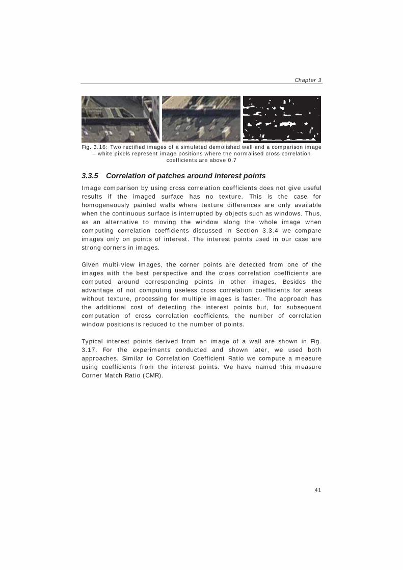
Chapter 3
41
Fig. 3.16: Two rectified images of a simulated demolished wall and a comparison image
– white pixels represent image positions where the normalised cross correlation coefficients are above 0.7
3.3.5 Correlation of patches around interest points Image comparison by using cross correlation coefficients does not give useful results if the imaged surface has no texture. This is the case for homogeneously painted walls where texture differences are only available when the continuous surface is interrupted by objects such as windows. Thus, as an alternative to moving the window along the whole image when computing correlation coefficients discussed in Section 3.3.4 we compare images only on points of interest. The interest points used in our case are strong corners in images. Given multi-view images, the corner points are detected from one of the images with the best perspective and the cross correlation coefficients are computed around corresponding points in other images. Besides the advantage of not computing useless cross correlation coefficients for areas without texture, processing for multiple images is faster. The approach has the additional cost of detecting the interest points but, for subsequent computation of cross correlation coefficients, the number of correlation window positions is reduced to the number of points. Typical interest points derived from an image of a wall are shown in Fig. 3.17. For the experiments conducted and shown later, we used both approaches. Similar to Correlation Coefficient Ratio we compute a measure using coefficients from the interest points. We have named this measure Corner Match Ratio (CMR).

Verification of 2D building outlines using oblique airborne images
42
Fig. 3.17: A rectified image of a wall and interest points extracted from the image and
used for cross correlation
3.3.6 Matching SIFT features For this measure we use the Scale-Invariant Feature Transform (SIFT) features (Lowe, 2004). SIFT feature matching is already a popular technique for identifying objects captured in different images. The features used are invariant to image scale, rotation and changes in illumination. For purpose of object recognition, the features captured in reference images are normally stored in a database and subsequent identification of an object is by comparing features in a new image to features in the database. In our case, SIFT features are detected from either of the rectified image portions of the wall hypothesis. Feature comparison is done for different image portions. In order to eliminate incorrect matches, the matching features are required to be within a small distance from each other. This is a means to filter outliers since both images are rectified to the same plane in object space. Fig. 3.18 shows SIFT features (left) on two rectified images of a wall and lines pointing to matched SIFT points before eliminating wrong matches (middle) and correct matches after eliminating the wrong matches (right). The SIFT Match Ratio (SMR) is computed as
(12)
Where are SIFT matches which are in similar positions and are the SIFT features from two image patches expected to contain the wall This is the ratio of the number of features correctly matched to the total number of SIFT features detected in any two image patches of the wall hypothesis. If there are more than two image patches, the overall ratio is obtained as the maximum from all of the comparisons.

Chapter 3
43
Fig. 3.18: SIFT features in two images (left), lines pointing on matched points - with
some wrong matches (middle) and wrong matches removed (right)
3.4 Combining evidence using Machine Learning methods
Given the evidence measures as discussed in Section 3.3.1 to 3.3.6, we are facing the problem of how to use these ratios to conclude that a wall exists or is demolished. Each of the evidences is weak. Thus, we use instances of features generated from a sample of objects appearing in some images to train a classifier and use the classifier for subsequent prediction of object classes. In the following classifiers used in this work are discussed.
3.4.1 Fuzzy set theory, Hint theory, Adaptive boosting and Random trees
Strategies for designing and implementing classifiers include fuzzy logic (Zadeh, 1965) which has been used in many works, some of the recent being (Carlsson and Fullér, 1996; Kumar et al., 2009; Sasikala and Petrou, 2001). When there is more than one type of evidence in support of the prediction of an object then a method for combining the evidence such as the Dempster–Shafer (D-S) theory of evidence (Dempster, 1967; Shafer, 1976) is required. A variant of the Dempster–Shafer theory called the Theory of Hints (Kohlas and Monney, 1995) allows different types of evidence to be combined as hints but, when information is missing, ignorance is also incorporated in the decision. Besides the non-stochastic fuzzy and D-S-approaches, statistic-based machine learning techniques are applied and compared in the framework of this research. These include decision trees ensembles in Adaptive Boosting (AdaBoost) (Freund and Schapire, 1997) and Random Trees (RTrees) (Breiman, 2001; Kuncheva, 2004; Maudes et al., 2012).

Verification of 2D building outlines using oblique airborne images
44
The AdaBoost algorithm makes many weak classifiers by using past observations. The weak classifiers used are simple, such as decision stumps. These are combined in a number of iterations, every time making weak hypotheses, weighting them, and in the next iteration concentrating on the samples that are wrongly classified. RTrees are a collection of tree predictors where the classification is done by obtaining a vote from every tree and then a choice is made for the class with majority of votes. For this research, we use and compare three approaches. In the first approach we use the fuzzy logic for obtaining the membership to "wall exists". Training samples are used to construct fuzzy membership functions for each of the measures computed from images. The existence of a wall is subsequently determined by combining memberships from different functions. The memberships are used as hints (Hints). For the second and third approach, the verification is done not by combining individual results but all training samples contribute to a combined classifier. The second approach is Adaptive Boosting (AdaBoost) and the third approach is the Random Trees (RTrees) classification method. The following section describes how fuzzy memberships are computed and the training and application of Hints, Adaptive boosting and Random trees.
3.4.2 Combining evidence Fuzzy membership functions: Using training data, the fuzzy
membership to the class “wall exists” at a given value of a measure is computed as the proportion of the number of existing walls to the total number of existing and demolished walls. The sizes of walls are used as weights. That is
(13)
Where are wall areas One of the ways that may be used to obtain membership functions is plotting verification ratios against memberships to make fuzzy membership curves. These curves are generalized to functions and used for subsequent verification. Practically, curves are generalised to concatenated linear functions with a linear increase and a constant as illustrated in Fig. 3.19. Only two values and need to be determined and then the two line segments are constructed as follows. The first is constructed as a line

Chapter 3
45
segment between points and , and the second is for all . For subsequent use of this function, all measures below return
memberships determined by the first segment while those above are assigned membership 1.0.
Fig. 3.19: Memberships modelled into a two line function.
In order to have a more automatic method the fuzzy membership functions were constructed from the training data in an automatic procedure. This was done by quantizing the verification ratios into a number of discrete small classes and obtaining membership for each of the classes. The results are stored as lookup table. Membership functions resulting from this procedure are given in Section 4.3. Combining Hints: We combine evidence from fuzzy membership functions using the Theory of Evidence. More specifically, we use the variant called the Theory of Hints (Kohlas and Monney, 1995). This combination takes into account ignorance. Consider an example where a wall is visible only in one image and thus facade edges are extracted in this image and can be tested for horizontal or vertical direction but no line comparison can be done. We can say that the line comparison gives no hint about the wall. In the context of hints this means ignorance is 1.0 while both support and plausibility are equal to 0.0. Adaptive Boosting and Random Trees: During AdaBoost training, all samples are assigned the same weight at the beginning and then the weights are increased for the samples wrongly classified. When the classifier has been trained, the prediction is done by combining responses from each weak classifier. The responses are either negative or positive. The overall classification for the two-class case is given by the sign of the weighted sum over the individual weak classifiers. Instead of binary class output, the likelihood between 0 and 1 can also be obtained. We compute this likelihood as the ratio of the sum of negative weights to the total of negative and positive responses. In this way, the likelihood around 0.5 implies that the training samples with features similar to the current wall were mixed for existing and demolished walls. These
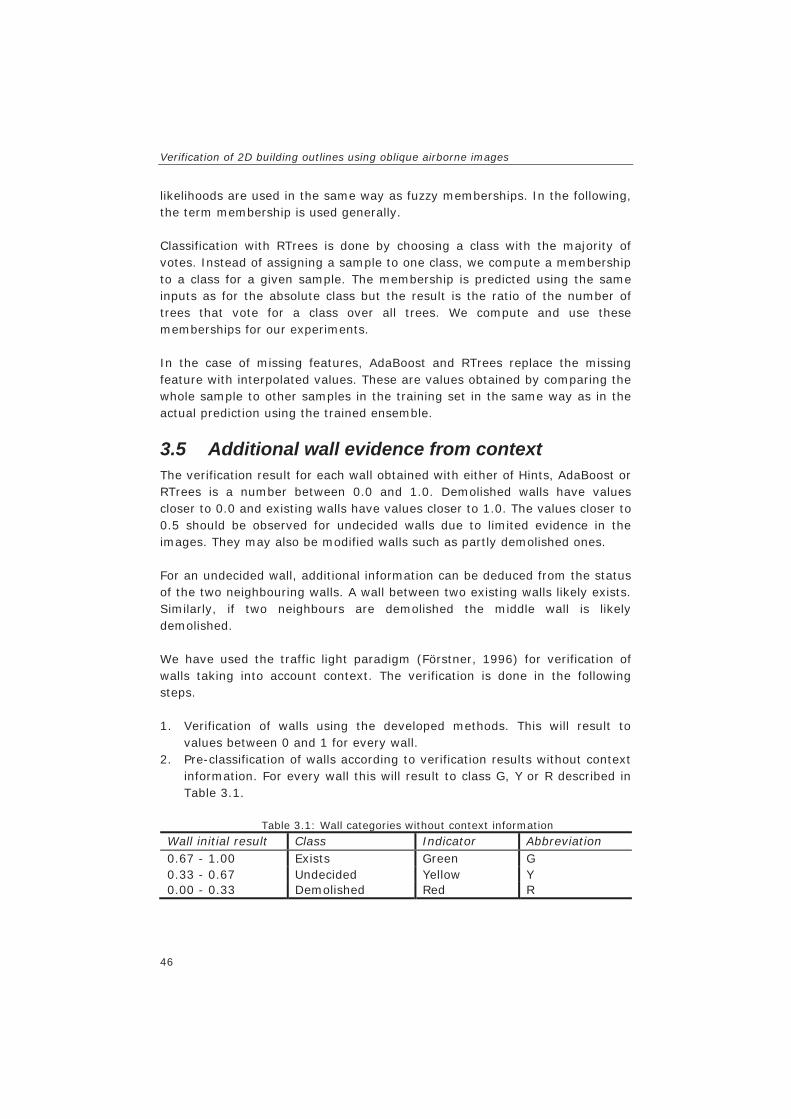
Verification of 2D building outlines using oblique airborne images
46
likelihoods are used in the same way as fuzzy memberships. In the following, the term membership is used generally. Classification with RTrees is done by choosing a class with the majority of votes. Instead of assigning a sample to one class, we compute a membership to a class for a given sample. The membership is predicted using the same inputs as for the absolute class but the result is the ratio of the number of trees that vote for a class over all trees. We compute and use these memberships for our experiments. In the case of missing features, AdaBoost and RTrees replace the missing feature with interpolated values. These are values obtained by comparing the whole sample to other samples in the training set in the same way as in the actual prediction using the trained ensemble.
3.5 Additional wall evidence from context The verification result for each wall obtained with either of Hints, AdaBoost or RTrees is a number between 0.0 and 1.0. Demolished walls have values closer to 0.0 and existing walls have values closer to 1.0. The values closer to 0.5 should be observed for undecided walls due to limited evidence in the images. They may also be modified walls such as partly demolished ones. For an undecided wall, additional information can be deduced from the status of the two neighbouring walls. A wall between two existing walls likely exists. Similarly, if two neighbours are demolished the middle wall is likely demolished. We have used the traffic light paradigm (Förstner, 1996) for verification of walls taking into account context. The verification is done in the following steps. 1. Verification of walls using the developed methods. This will result to
values between 0 and 1 for every wall. 2. Pre-classification of walls according to verification results without context
information. For every wall this will result to class G, Y or R described in Table 3.1.
Table 3.1: Wall categories without context information
Wall initial result Class Indicator Abbreviation 0.67 - 1.00 Exists Green G 0.33 - 0.67 Undecided Yellow Y 0.00 - 0.33 Demolished Red R

Chapter 3
47
3. Classification of walls using initial verification results and context information. In this step, walls that are categorised as Y are re-classified by taking into consideration the class of the two adjacent walls of the same building by using simple rules as shown in Table 3.2 below.
Table 3.2: Wall categories with context information
Initial class Classes of neighbouring walls Class with Context G Both in any class G, R or Y G R Both in any class G, R or Y R Y Both G G Y Both R R Y One R and other G Y Y Both Y Y
For purpose of utilising context information, all invisible walls are assigned to the undecided class (Y) during the pre-classification step (step 2). Therefore, if both walls neighbouring an invisible wall are in class G or R then the invisible wall is classified as G or R respectively.
3.6 Combining wall evidence per-building After wall verification, each of the buildings with walls categorised as demolished may be presented to the operator for updating. The results per wall can also be used to obtain the overall building status. The building status may be decided by combining results from the individual walls by using a set of rules such as if all walls are classified as G then the building is categorised as unchanged. A set of rules used for combining results in our case are as shown in Table 3.3. When all walls are undecided (class Y), the building is undecided. This may happen in instances such as when a building is completely occluded or there is equal evidence for and against existence of the wall.
Table 3.3: Building categories according to wall results
Wall results Expression Building category All walls Y 0RG ##
Undecided
At least 80% of walls are G 80.
###
RGG
Building not changed
At least 80% of walls are R 80.
###
RGR
Building is demolished
R and G walls Else Building is modified (extended or part demolished)
As discussed in Section 3.5, all invisible walls are assigned to the undecided class (Y) during the pre-classification step. When context information is used

Verification of 2D building outlines using oblique airborne images
48
these walls are assigned Y, G or R depending on the state of the neighbours. If all walls of a building are invisible, all its walls will be in class Y and the building will be undecided. If some walls are visible, a building category is based on the visible walls only and then the building will be classified as not changed, demolished or modified depending on the number of the G and R walls. By using context information in verification of a wall the overall result is improved. However, this approach suffers when the evidence from some walls of a building are erroneously categorised as existing or demolished (R or G) in the pre-classification stage. The building will ultimately be categorised as modified if we apply a strict rule that categorises a building as modified even when results from only one wall are contrary to other walls. For illustration, consider a building with four walls which are not demolished or changed in reality. Suppose the walls initial verification results are 0.9, 0.9, 0.1, and 0.9. The third wall result is incorrect. The pre-classification results will be G, G, R and G and the classification using context will not change these classes. The overall building category will be building is modified. This happens because the classification of the third wall is strongly erroneous. This kind of wrong categorisation of buildings is encountered, for buildings with many walls coupled with less evidence from images due to unavailability of multiple views and occlusion. For taking this problem into account a small tolerance is allowed (Table 3.3).
3.7 Discussion Our approach verifies walls individually and combines results for whole buildings. Each of Hints, AdaBoost and RTrees results to a value between 0.0 and 1.0 for each visible wall. The final result per wall is obtained by taking into account the state of the neighbours. A wall is ultimately categorised as existing, demolished or undecided and the per-wall results are combined for the whole buildings. The following aspects of the method are important to note. The measures used for verification of walls are correlated weak classifiers. For example, if a wall has some horizontal or vertical facade edges, these edges will be detected in the images and will results to the Line Direction Ration close to 1.0. At the same time, when comparing lines from different images, the Line Match Ratio will likely be close to 1.0 due to the availability of the same vertical and horizontal edges. Similarly, the Sift Match Ratio is

Chapter 3
49
related to Corner Match Ratio and Cross Correlation Ratio as they all depend on wall facade features such as colour difference and corners. An important feature of our method is dependency on multi-view or overlap images. With exception of Line Direction Ratio, all measures used for verification of a wall require more than one image. When only one image is available for a wall, the Line Match Ratio can be used alone but the result is more uncertain. Another aspect is the impact of occlusion. Walls that are occluded by other buildings or trees cannot be verified. A building with only a few of its walls visible is verified only basing on the visible walls which may not necessarily be correct. Other problems of the method are related to the wall hypothesis verified. A wall is assumed to be vertical and planar. Thus, confusion arises for non-vertical and round walls.

Verification of 2D building outlines using oblique airborne images
50
51
4. Experimental verification of 2D building outlines
4.1 Experimental design The purpose of experiments discussed in this chapter is to evaluate the performance of the method developed for verification of 2D building outlines. The intention is to:
Examine completeness and correctness of verification of existing buildings;
Examine completeness and correctness of verification of demolished buildings;
Find out if there are added benefits when verification is done by using image datasets with high overlap and resolution.
To analyse the benefit of using context information instead of individual wall information;
To identify causes of errors in the verification;
To examine the results obtained per building when wall results are combined. The analysis was done for unchanged, demolished and modified buildings;
To check if training done by using one image dataset can be useful for verification by using another image dataset;
To check if training with buildings from one area (e.g. one city) can be useful for verification of buildings in another area.
To achieve these objectives, we used test datasets of building outlines and oblique images. The building outlines represent the old situation and the oblique images represent the current situation to which the building outlines are compared against. We needed to conduct the experiments with sample datasets containing many existing, demolished and changed buildings. While changes due to disasters such as fire, flooding or earthquake, usually cause many changes within a short period of time, urban redevelopment takes place continuously but with few changes over a small period of time. Many existing buildings are visible in the images while only a few demolished ones are noticeable. Thus, additional demolished buildings were obtained by simulation. The simulation was done by shifting the 2D building outlines of existing buildings to other arbitrary places.
Experimental verification of 2D building outlines
52
Building outlines used for experiments were divided into two samples. One sample was used for training and the other for validation. The training dataset was used to derive evidence from images and construct the fuzzy membership functions required for the Hints method. It was also used for training AdaBoost and RTree classifiers. Experiments were conducted using the three methods and results were compared.
4.2 Data description
4.2.1 Buildings verified Building verification experimentation was done with two applications in mind. The first application is map updating and the second is damage assessment. Two building datasets were also chosen, one for each application. Map updating: the intention is to confirm correctness of the buildings in the map data and to identify normal changes due to urban redevelopment. These changes are effected in between the map data captured and the acquisition of the images that are used for the verification. With this purpose in mind, we selected an urban area and verified the buildings defined by map data. The data used is a portion of the large scale topographic dataset of the Netherlands (GBKN) covering a part of the city of Enschede. Damage assessment: the purpose is to identify buildings that may have been destructed due to a disaster such as earth quake, fire or tsunami. The purpose of building verification after a disaster, such as an earth quake, is to aid rapid damage mapping. The verification helps to identify the buildings that are unchanged, demolished or partly destructed. For this purpose we selected a part of Port-au-Prince, Haiti. In the following, the Enschede and Haiti datasets are briefly described. Enschede data: For this study we used 652 building outlines in the topographic dataset. The outlines are very detailed with position accuracy estimated at around 10-20 cm standard deviation. The data is suitable for large scale maps (Fig. 4.1). In the original topographic data, some line segments are broken into segments representing different apartments. To obtain lines for the whole walls, we removed every middle point of any three consecutive nodes that are collinear. Haiti data: The images used for verification were captured immediately after the earth quake that occurred on 12th January, 2010. The vector dataset verified represents buildings as they were before the disaster. Fig.
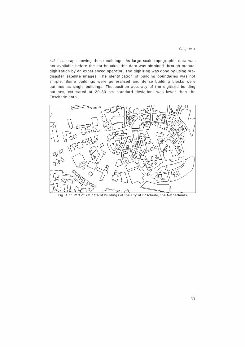
Chapter 4
53
4.2 is a map showing these buildings. As large scale topographic data was not available before the earthquake, this data was obtained through manual digitization by an experienced operator. The digitizing was done by using pre-disaster satellite images. The identification of building boundaries was not simple. Some buildings were generalised and dense building blocks were outlined as single buildings. The position accuracy of the digitised building outlines, estimated at 20-30 cm standard deviation, was lower than the Enschede data.
Fig. 4.1: Part of 2D data of buildings of the city of Enschede, the Netherlands
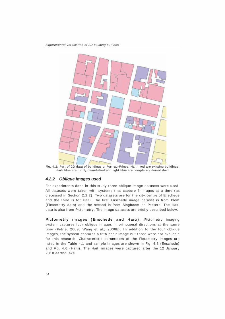
Experimental verification of 2D building outlines
54
Fig. 4.2: Part of 2D data of buildings of Port-au-Prince, Haiti: red are existing buildings,
dark blue are partly demolished and light blue are completely demolished
4.2.2 Oblique images used For experiments done in this study three oblique image datasets were used. All datasets were taken with systems that capture 5 images at a time (as discussed in Section 2.2.2). Two datasets are for the city centre of Enschede and the third is for Haiti. The first Enschede image dataset is from Blom (Pictometry data) and the second is from Slagboom en Peeters. The Haiti data is also from Pictometry. The image datasets are briefly described below. Pictometry images (Enschede and Haiti): Pictometry imaging system captures four oblique images in orthogonal directions at the same time (Petrie, 2009; Wang et al., 2008b). In addition to the four oblique images, the system captures a fifth nadir image but those were not available for this research. Characteristic parameters of the Pictometry images are listed in the Table 4.1 and sample images are shown in Fig. 4.3 (Enschede) and Fig. 4.6 (Haiti). The Haiti images were captured after the 12 January 2010 earthquake.
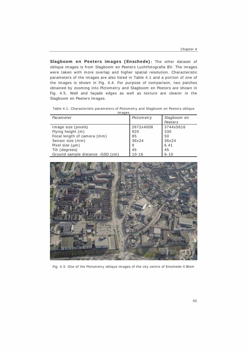
Chapter 4
55
Slagboom en Peeters images (Enschede): The other dataset of oblique images is from Slagboom en Peeters Luchtfotografie BV. The images were taken with more overlap and higher spatial resolution. Characteristic parameters of the images are also listed in Table 4.1 and a portion of one of the images is shown in Fig. 4.4. For purpose of comparison, two patches obtained by zooming into Pictometry and Slagboom en Peeters are shown in Fig. 4.5. Wall and façade edges as well as texture are clearer in the Slagboom en Peeters images.
Table 4.1: Characteristic parameters of Pictometry and Slagboom en Peeters oblique images
Parameter Pictometry Slagboom en Peeters
Image size (pixels) 2672x4008 3744x5616 Flying height (m) 920 330 Focal length of camera (mm) 85 50 Sensor size (mm) 36x24 36x24 Pixel size ( m) 9 6.41 Tilt (degrees) 45 45 Ground sample distance -GSD (cm) 10-16 6-10
Fig. 4.3. One of the Pictometry oblique images of the city centre of Enschede ©Blom

Experimental verification of 2D building outlines
56
Fig. 4.4: One of the Slagboom en Peeters oblique images of the city centre of Enschede
Fig. 4.5: Zoom into images in fig Fig. 4.3 and Fig. 4.4 showing the same building –
top: Pictometry and bottom: Slagboom en Peeters

Chapter 4
57
Fig. 4.6: One of the Pictometry oblique images of Haiti (above) and a zoom into the
image (bottom) For all datasets, the exterior and interior orientation parameters were obtained by incorporating scene constraints in the triangulation of oblique
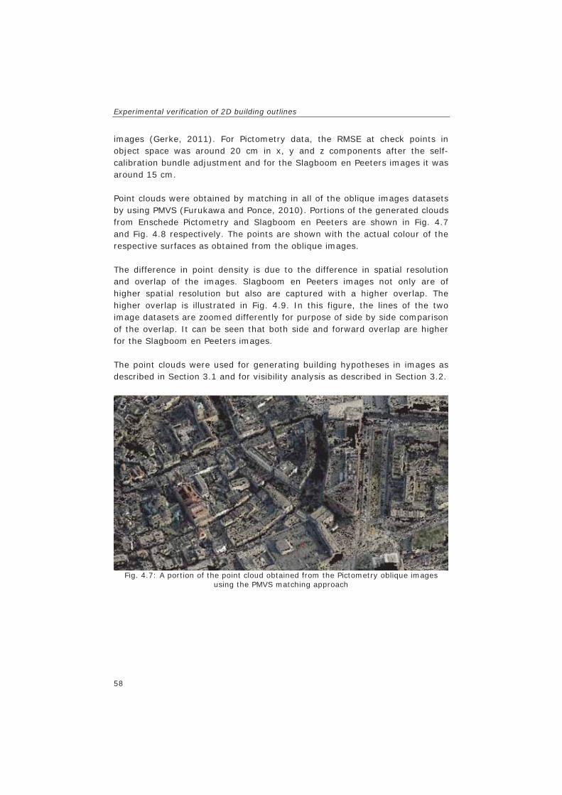
Experimental verification of 2D building outlines
58
images (Gerke, 2011). For Pictometry data, the RMSE at check points in object space was around 20 cm in x, y and z components after the self-calibration bundle adjustment and for the Slagboom en Peeters images it was around 15 cm. Point clouds were obtained by matching in all of the oblique images datasets by using PMVS (Furukawa and Ponce, 2010). Portions of the generated clouds from Enschede Pictometry and Slagboom en Peeters are shown in Fig. 4.7 and Fig. 4.8 respectively. The points are shown with the actual colour of the respective surfaces as obtained from the oblique images. The difference in point density is due to the difference in spatial resolution and overlap of the images. Slagboom en Peeters images not only are of higher spatial resolution but also are captured with a higher overlap. The higher overlap is illustrated in Fig. 4.9. In this figure, the lines of the two image datasets are zoomed differently for purpose of side by side comparison of the overlap. It can be seen that both side and forward overlap are higher for the Slagboom en Peeters images. The point clouds were used for generating building hypotheses in images as described in Section 3.1 and for visibility analysis as described in Section 3.2.
Fig. 4.7: A portion of the point cloud obtained from the Pictometry oblique images
using the PMVS matching approach

Chapter 4
59
Fig. 4.8: A portion of the point cloud obtained from the Slagboom en Peeters images
using the PMVS matching approach
Fig. 4.9: Overlap of Enschede Pictometry and Slagboom en Peeters images –
consecutive image samples from east facing camera of Pictometry (left) and Slagboom en Peeters (right)
4.3 Training AdaBoost, RTrees and fuzzy membership functions
The training and validation was done by using verification measures computed by using oblique images and existing and demolished buildings outlines as discussed in Section 3.3. The verification measures were computed for all walls and then different training and validation sets composed a number of times, each by selecting half of the walls as a training set and the other half as a validation set.

Experimental verification of 2D building outlines
60
Before computation of the verification measures, occluded walls were automatically isolated and walls visible from one perspective were used for obtaining the Line Direction and Building Edge Ratios only as other measures require the availability of at least two images. For AdaBoost and RTrees training, the inputs are the actual measures derived from the images for all the training walls together with the corresponding state (exists or demolished). For classification with Hints verification measures were used to obtain fuzzy membership functions. Functions were constructed for each of the measures independently. Different membership curves obtained are shown in Fig. 4.10 (Enschede Pictometry), in Fig. 4.11 (Enschede Slagboom en Peeters) and Fig. 4.12 (Haiti). The respective membership values were automatically generated as discussed in Section 3.4.2.
00.10.20.30.40.50.60.70.80.9
1
0 0.1 0.2 0.3 0.4 0.5 0.6 0.7 0.8 0.9 1
Measure
Mem
bers
hip
LMRLDRSMRCCRCMRBER
Fig. 4.10: Fuzzy memberships automatically generated for training with Enschede
Pictometry images: x-axis for measures and y-axis for the memberships to class “wall exists” - LMR for Line Match Ratio, LDR for Line Direction Ratio, SMR for SIFT match ratio, CCR for Correlation Coefficient Ratio, CMR for Corner Match Ratio and BER for
Building Edge Ratio
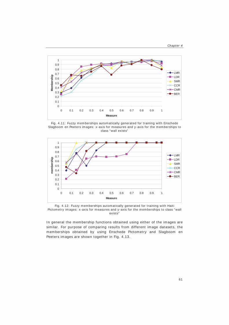
Chapter 4
61
00.10.20.30.40.50.60.70.80.9
1
0 0.1 0.2 0.3 0.4 0.5 0.6 0.7 0.8 0.9 1
Measure
Mem
bers
hip
LMRLDRSMRCCRCMRBER
Fig. 4.11: Fuzzy memberships automatically generated for training with Enschede
Slagboom en Peeters images: x-axis for measures and y-axis for the memberships to class “wall exists”
00.10.20.30.40.50.60.70.80.9
1
0 0.1 0.2 0.3 0.4 0.5 0.6 0.7 0.8 0.9 1
Measure
mem
bers
hip
LMRLDRSMRCCRCMRBER
Fig. 4.12: Fuzzy memberships automatically generated for training with Haiti
Pictometry images: x-axis for measures and y-axis for the memberships to class “wall exists”
In general the membership functions obtained using either of the images are similar. For purpose of comparing results from different image datasets, the memberships obtained by using Enschede Pictometry and Slagboom en Peeters images are shown together in Fig. 4.13.
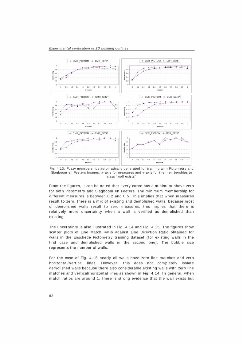
Experimental verification of 2D building outlines
62
0
0.2
0.4
0.6
0.8
1
0 0.1 0.2 0.3 0.4 0.5 0.6 0.7 0.8 0.9 1
measure
mem
bers
hip
LMR_PICTOM LMR_SENP
0
0.2
0.4
0.6
0.8
1
0 0.1 0.2 0.3 0.4 0.5 0.6 0.7 0.8 0.9 1
measure
mem
bers
hip
LDR_PICTOM LDR_SENP
0
0.2
0.4
0.6
0.8
1
0 0.1 0.2 0.3 0.4 0.5 0.6 0.7 0.8 0.9 1
measure
mem
bers
hip
SMR_PICTOM SMR_SENP
0
0.2
0.4
0.6
0.8
1
0 0.1 0.2 0.3 0.4 0.5 0.6 0.7 0.8 0.9 1
measurem
embe
rshi
p
CCR_PICTOM CCR_SENP
0
0.2
0.4
0.6
0.8
1
0 0.1 0.2 0.3 0.4 0.5 0.6 0.7 0.8 0.9 1
measure
mem
bers
hip
CMR_PICTOM CMR_SENP
0
0.2
0.4
0.6
0.8
1
0 0.1 0.2 0.3 0.4 0.5 0.6 0.7 0.8 0.9 1
measure
mem
bers
hip
BER_PICTOM BER_SENP
Fig. 4.13: Fuzzy memberships automatically generated for training with Pictometry and Slagboom en Peeters images: x-axis for measures and y-axis for the memberships to
class “wall exists” From the figures, it can be noted that every curve has a minimum above zero for both Pictometry and Slagboom en Peeters. The minimum membership for different measures is between 0.2 and 0.5. This implies that when measures result to zero, there is a mix of existing and demolished walls. Because most of demolished walls result to zero measures, this implies that there is relatively more uncertainty when a wall is verified as demolished than existing. The uncertainty is also illustrated in Fig. 4.14 and Fig. 4.15. The figures show scatter plots of Line Match Ratio against Line Direction Ratio obtained for walls in the Enschede Pictometry training dataset (for existing walls in the first case and demolished walls in the second one). The bubble size represents the number of walls. For the case of Fig. 4.15 nearly all walls have zero line matches and zero horizontal/vertical lines. However, this does not completely isolate demolished walls because there also considerable existing walls with zero line matches and vertical/horizontal lines as shown in Fig. 4.14. In general, when match ratios are around 1, there is strong evidence that the wall exists but

Chapter 4
63
match ratios around 0 give weak evidence for identifying demolished buildings.
-0.2
0
0.2
0.4
0.6
0.8
1
-0.2 0 0.2 0.4 0.6 0.8 1
Fig. 4.14: The relationship between LMR and LDR (existing walls)
-0.2
0
0.2
0.4
0.6
0.8
1
-0.2 0 0.2 0.4 0.6 0.8 1
LMR
LDR
Fig. 4.15: The relationship between LMR and LDR (demolished walls)

Experimental verification of 2D building outlines
64
4.4 Evaluation criteria The null-hypothesis constructed for every wall is “the wall exists”. The decisions we can make are illustrated in (Table 4.2). Correctly verified walls are true positives (TP) and demolished walls identified are true negatives (TN). There are two types of wrong decisions we can make in verifying a wall. Walls wrongly decided as existing when actually they are demolished are false positives (FP) and walls decided as demolished when they still exist are false negatives (FN). Table 4.2: Possible state of walls in reality and in verification results – solid and dashed
lines represent existing and demolished walls respectively Reality Verification result Decision type TP FN
FP
TN
Results obtained with experiments are used to form a confusion matrix. The values in the matrix are used to compute four evaluation ratios as follows:
(14)
(15)
(16)
(17)
The Completeness_Exists is the proportion of correctly verified walls among all existing walls in the sample and the Completeness_Demolished is the proportion of demolished walls identified among all demolished walls in the sample. The Correctness_Exists is the number of walls correctly verified among all walls categorised as existing and Correctness_Demolished is the number of demolished walls correctly identified among all walls identified as demolished.

Chapter 4
65
4.5 Wall verification results In the following sections results are presented including the proportions of existing and demolished walls that are correctly identified. The results are shown for the evidence combination methods: Hints, AdaBoost and RTrees for comparison purpose. The results for Pictometry and Slagboom en Peeters images over the same building dataset serves to know the effect of higher overlap and spatial resolution of the images used in the verification. The Enschede and Haiti building outlines are used as two main application areas of the developed method: identification of changes due to urban redevelopment and buildings affected by disasters.
4.5.1 Quantitative results with Enschede Pictometry images The numbers of walls used for verification using Enschede Pictometry images are as shown in Table 4.3. We obtained results for existing walls as shown in the Fig. 4.16. The figure shows the distribution of memberships to ‘wall exists’ obtained by using Hints, AdaBoost and RTrees. These results are as obtained per wall before using context information (described in Section 3.5). In the horizontal axis are the memberships and in the vertical axis are the numbers of walls. Notice that most of the wall memberships are close to 1.0 implying the walls are correctly categorized as existing. The distribution of memberships to ‘wall exists’ for demolished walls is shown on Fig. 4.17. Most of the wall memberships are close to zero implying the walls are correctly categorized as demolished.
Table 4.3: Walls verified with Enschede Pictometry images Visible walls Invisible walls Existing walls 6881 4663 Demolished walls 6245 5688
It was noted that the RTrees approach tends to categorise most results either to 0.0 or 1.0. Most walls correctly categorised as existing result to membership 1.0 (see the strong peak in Fig. 4.16) but also there are more walls wrongly classified as demolished (at 0.0) than AdaBoost and Hints. Similarly, most walls correctly categorised as demolished result to membership 0.0 (see the strong peak in Fig. 4.17) but also there are more walls wrongly classified as existing (at 1.0) than AdaBoost and Hints.

Experimental verification of 2D building outlines
66
0
10
20
30
40
50
60
70
80
<=0.1 0.2 0.3 0.4 0.5 0.6 0.7 0.8 0.9 1
Membership
% w
alls AdaBoost
RtreesHints
Fig. 4.16: Membership to ‘wall exists’ for existing walls in validation data – verification
with Enschede Pictometry images
0
510
15
2025
30
3540
45
<=0.1 0.2 0.3 0.4 0.5 0.6 0.7 0.8 0.9 1
Membership
% w
alls AdaBoost
RtreesHints
Fig. 4.17: Memberships to ‘wall exists’ for demolished walls in validation data –
verification with Enschede Pictometry images Quantitative results from experiments using Enschede Pictometry images are shown in Table 4.4 for completeness and Table 4.5 for correctness. In both tables the results obtained by using individual walls (where a wall is categorised as existing if membership is above 0.5) are provided against results obtained by using context information (as described in Section 3.5 ). It was noted that the completeness and correctness obtained by using context information are higher than without context information. This shows that the context information is useful. For example completeness of existing walls, using AdaBoost and Enschede Pictometry images, improved from 93% to 95% when context was taken into account.

Chapter 4
67
It was also noted that results from AdaBoost were better than RTrees and Hints. AdaBoost was followed by RTrees and Hints results were relatively lowest. The better results from AdaBoost were likely due to less existing walls that are classified close to membership 0.1. Table 4.4: Wall verification results (completeness) obtained with Enschede Pictometry
images
Method Completeness_Existing Without/with context
Completeness_Demolished Without/with context
Hints 83% 85% 76% 77% AdaBoost 93% 95% 88% 89% RTrees 87% 88% 79% 80%
Table 4.5: Wall verification results (correctness) obtained with Enschede Pictometry
images
Method Correctness_ Existing Without/with context
Correctness_ Demolished Without/with context
Hints 85% 86% 74% 77% AdaBoost 93% 94% 88% 90% RTrees 86% 87% 80% 82%
4.5.2 Quantitative results with Enschede Slagboom en Peeters images
By using Slagboom en Peeters images, we obtained verification results for existing walls as shown in the Fig. 4.18. These results were obtained from walls shown in Table 4.6. The wall memberships are also close to 1.0 implying the walls are correctly categorized as existing.
Table 4.6: Walls verified with Slagboom en Peeters images Visible walls Invisible walls Existing walls 3321 3326 Demolished walls 2769 4011
The distribution of memberships to ‘wall exists’ for demolished walls is also shown on Fig. 4.19. Notice that most of the wall memberships are close to zero implying the walls are correctly categorized as demolished.
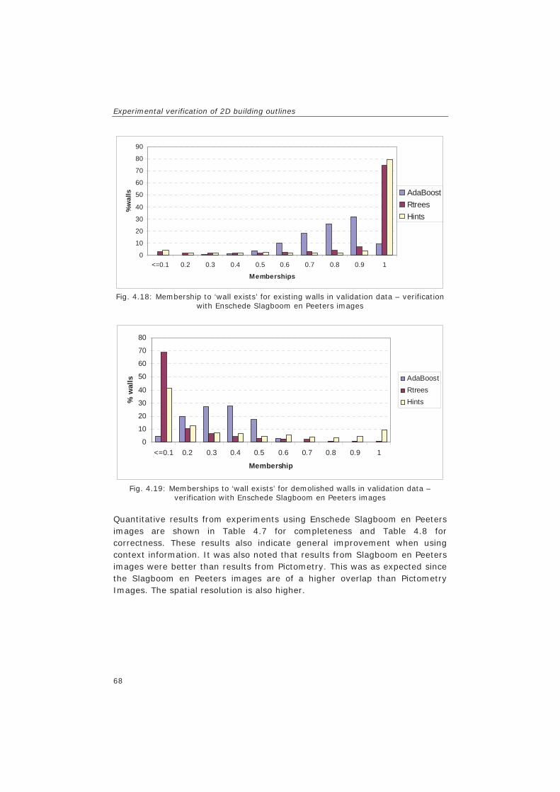
Experimental verification of 2D building outlines
68
0
10
20
30
40
50
60
70
80
90
<=0.1 0.2 0.3 0.4 0.5 0.6 0.7 0.8 0.9 1
Memberships
%w
alls AdaBoost
RtreesHints
Fig. 4.18: Membership to ‘wall exists’ for existing walls in validation data – verification
with Enschede Slagboom en Peeters images
0
10
20
30
40
50
60
70
80
<=0.1 0.2 0.3 0.4 0.5 0.6 0.7 0.8 0.9 1
Membership
% w
alls AdaBoost
RtreesHints
Fig. 4.19: Memberships to ‘wall exists’ for demolished walls in validation data –
verification with Enschede Slagboom en Peeters images Quantitative results from experiments using Enschede Slagboom en Peeters images are shown in Table 4.7 for completeness and Table 4.8 for correctness. These results also indicate general improvement when using context information. It was also noted that results from Slagboom en Peeters images were better than results from Pictometry. This was as expected since the Slagboom en Peeters images are of a higher overlap than Pictometry Images. The spatial resolution is also higher.

Chapter 4
69
Table 4.7:Wall verification results (completeness) obtained with Enschede Slagboom en Peeters images
Method Completeness_Existing Without/with context
Completeness_Demolished Without/with context
Hints 88% 92% 73% 79% AdaBoost 95% 99% 97% 99% RTrees 95% 94% 95% 97%
Table 4.8: Wall verification results (correctness) obtained with Enschede Slagboom en
Peeters images
Method Correctness_ Existing Without/with context
Correctness_ Demolished Without/with context
Hints 81% 87% 81% 86% AdaBoost 98% 99% 93% 99% RTrees 97% 98% 93% 92%
4.5.3 Quantitative results with Haiti Pictometry images Haiti data was much different from Enschede data. The building outlines and the image orientation were of less geometric accuracy. The vector data obtained by digitizing in pre-disaster satellite images in some cases did not fit well with the images. With Haiti data, we obtained verification results for existing walls as shown in the Fig. 4.20. The numbers of verified walls are as in Table 4.9. The distribution indicates the difficulty of separating existing and demolished wall in this case. Those walls with membership 0.5 were wrongly categorized as demolished.
Table 4.9: Walls verified in Haiti data Visible walls Invisible walls Existing walls 209 79 Demolished walls 31 5
The distribution of memberships to ‘wall exists’ for demolished walls is also shown on Fig. 4.21. Notice that most of the wall memberships are below 0.5 indicating that most walls are correctly categorized as demolished. The memberships above 0.5 are also higher, relative to the Enschede cases, indicating a higher level of categorising demolished walls as existing.

Experimental verification of 2D building outlines
70
05
101520253035404550
0.1 0.2 0.3 0.4 0.5 0.6 0.7 0.8 0.9 1
Membership
% w
alls AdaBoost
RtreesHints
Fig. 4.20: Memberships to ‘wall exists’ for existing walls in validation data – verification
with Haiti Pictometry images
0
10
20
30
40
50
60
70
0.1 0.2 0.3 0.4 0.5 0.6 0.7 0.8 0.9 1
Membership
% w
alls AdaBoostRtreesHints
Fig. 4.21: Memberships to ‘wall exists’ for demolished walls in validation data –
verification with Haiti Pictometry images Quantitative results of experiments with Haiti data are shown in Table 4.10 for completeness and Table 4.11 for correctness. The few existing and demolished buildings digitized (shown in red and light blue in Fig. 4.2) were used for a number of experiments each time by picking different walls for training and validation. The results shown in the tables were obtained by combining results from all the experiments.

Chapter 4
71
Table 4.10: Wall verification results (completeness) obtained with Haiti Pictometry images
Method Completeness_Existing Without/with context
Completeness_Demolished Without/with context
Hints 63% 71% 72% 81% AdaBoost 54% 59% 76% 81% RTrees 55% 57% 76% 84%
Table 4.11: Wall verification results (correctness) obtained with Haiti Pictometry
images
Method Correctness_ Existing Without/with context
Correctness_ Demolished Without/with context
Hints 69% 78% 72% 73% AdaBoost 69% 75% 62% 66% RTrees 70% 78% 63% 66%
As can be seen the results were worse than with Enschede data due to the problems of the quality of the image orientation and the position accuracy of the digitized building outlines. The number of walls that was used for verification experiments in the Haiti case was also quite small. Fig. 4.22 is one example. A wall expected in two images is shown on rectified patches (top). The rectified patches differ due to errors in image orientation and the position of the wall. Sift features were generated from both images (middle) but none matched (bottom).
Fig. 4.22: A wall in two images (top) where the rectified images differ due to errors in image orientation and the position of the wall, Sift features were generated (middle)
but none matched (bottom)

Experimental verification of 2D building outlines
72
4.5.4 Qualitative wall verification results Some errors are discussed in the following. One type of error is due to the differences of walls at different floors of the same building. Fig. 4.23 shows a small part of a building for which the ground and upper floor of the building differs. The map represents the ground floor. Because the data being verified is in 2D there is no way to limit the verification to a portion of a building defined by height. The wall is categorized as demolished.
Fig. 4.23: A wall with different geometry at ground and upper floors, only the ground
floor is captured in the map Another problem relates to failure in visibility analysis. An existing wall results to low line match ratio as well as other measures when a wall is not visible but is not identified as such during the visibility analysis stage. This happens, if a point cloud used for visibility analysis has none or very few points directly in front of the tested wall when actually the wall is occluded. In these cases, a wall that should be excluded from the verification due to occlusion is included. This problem is illustrated in Fig. 4.24. The vegetation in front of the building in the left image was not identified during visibility analysis. As a result, lines detected in the right image could not match with any line in the left image.
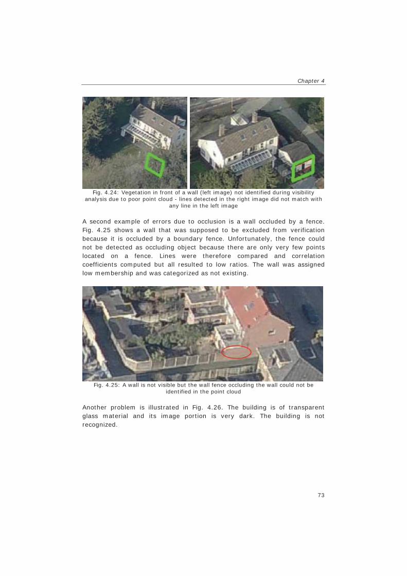
Chapter 4
73
Fig. 4.24: Vegetation in front of a wall (left image) not identified during visibility
analysis due to poor point cloud - lines detected in the right image did not match with any line in the left image
A second example of errors due to occlusion is a wall occluded by a fence. Fig. 4.25 shows a wall that was supposed to be excluded from verification because it is occluded by a boundary fence. Unfortunately, the fence could not be detected as occluding object because there are only very few points located on a fence. Lines were therefore compared and correlation coefficients computed but all resulted to low ratios. The wall was assigned low membership and was categorized as not existing.
Fig. 4.25: A wall is not visible but the wall fence occluding the wall could not be
identified in the point cloud Another problem is illustrated in Fig. 4.26. The building is of transparent glass material and its image portion is very dark. The building is not recognized.

Experimental verification of 2D building outlines
74
Fig. 4.26: The small building is not recognized because it is of transparent materials
that resulted to a dark image The verification also fails when walls are not planar. This problem is illustrated in Fig. 4.27. The tower is cylindrical, with a circular footprint. The footprint is represented by 61 connected lines in the database. Some of these lines were combined to one wall during the process of combining collinear nodes discussed in Section 4.2. The resulting planar hypotheses could not be verified.
Fig. 4.27: Walls of a building not planar and could not be verified using our planar wall
hypothesis Other errors occur when walls are not vertical. This problem is illustrated in Fig. 4.28. The data from which we construct our wall is in 2D and hypotheses constructed are only for vertical walls. When the vertical wall is projected to images, it falls in a different area from the area covered by the actual slanting wall. When projected in an image from a different perspective, it falls in another image area. Thus both measures obtained from individual images

Chapter 4
75
as well as those computed by using multiple images will be incorrect. Walls that are not vertical are therefore not verifiable.
Fig. 4.28: A wall is not vertical and was not recognized because our hypothesis is for
vertical walls. In the case of Line Match Ratio, an existing wall results to low line match ratio when lines detected in images of different perspectives correspond to different façade edges. For example, if some horizontal façade edges such as on window frames are detected in the first image while different edges such as vertical building edges are detected in the second image, the two line sets will not match when compared. This happens due to the difference in image perspectives and thresholds used in line detection.
4.6 Building verification results
4.6.1 Results for unchanged and demolished building A building is categorised as not changed, demolished or modified depending on the verification results of its walls as discussed in Section 3.6. A building may also be categorised as undecided if no evidence was obtained for its walls, such as when the building is completely occluded by other buildings. The rules for the classification of a building are discussed in Section 3.6. Fig. 4.29 shows a sample of the buildings categorised as undecided due to occlusion. The vector data verified contained some polygons that represent different partitions of a building, captured for administration or tax purposes, but are part of the same building. During visibility analysis these were identified and excluded. They are therefore excluded in the results discussed in this section.

Experimental verification of 2D building outlines
76
Fig. 4.29: Buildings categorised as undecided (represented in red) are mainly due to
occlusion Experiments presented in Section 4.5 were for unchanged or completely demolished buildings at per wall level. This section presents the same results combined per building. In order to obtain results for extended or partly demolished buildings, some building outlines were modified and tested separately. These extended or partly demolished buildings are discussed later in Section 0. The per-building results for unchanged and demolished buildings are shown in Table 4.12 for Enschede Pictometry images, Table 4.13 for Enschede Slagboom en Peeters images and Table 4.14 for Haiti Pictometry images. For Enschede data, most existing buildings were correctly categorised. For example, when using AdaBoost, unchanged buildings verified in Enschede Pictometry and Enschede Slagboom en Peeters were 88%, 99% respectively while 10% and 1% buildings were categorised as modified. Similarly, most demolished buildings were labelled correctly for Enschede data. For example, when using AdaBoost, demolished buildings identified in Pictometry and Slagboom en Peeters images were 79% and 99% respectively while 13% and 0% buildings were categorised as modified. It was noted that results from Slagboom en Peeters were generally better than Pictometry. This was as expected because the Slagboom en Peeters images were of higher overlap and higher spatial resolution.
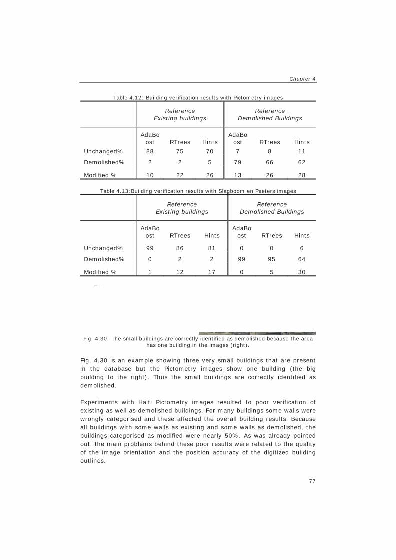
Chapter 4
77
Table 4.12: Building verification results with Pictometry images
Reference Existing buildings
Reference Demolished Buildings
AdaBoost RTrees Hints
AdaBoost RTrees Hints
Unchanged% 88 75 70 7 8 11
Demolished% 2 2 5 79 66 62
Modified % 10 22 26 13 26 28
Table 4.13:Building verification results with Slagboom en Peeters images
Reference Existing buildings
Reference Demolished Buildings
AdaBoost RTrees Hints
AdaBoost RTrees Hints
Unchanged% 99 86 81 0 0 6
Demolished% 0 2 2 99 95 64
Modified % 1 12 17 0 5 30
Fig. 4.30: The small buildings are correctly identified as demolished because the area
has one building in the images (right). Fig. 4.30 is an example showing three very small buildings that are present in the database but the Pictometry images show one building (the big building to the right). Thus the small buildings are correctly identified as demolished. Experiments with Haiti Pictometry images resulted to poor verification of existing as well as demolished buildings. For many buildings some walls were wrongly categorised and these affected the overall building results. Because all buildings with some walls as existing and some walls as demolished, the buildings categorised as modified were nearly 50%. As was already pointed out, the main problems behind these poor results were related to the quality of the image orientation and the position accuracy of the digitized building outlines.

Experimental verification of 2D building outlines
78
Table 4.14: Building verification results with Haiti buildings and Pictometry images
Reference Existing buildings
Reference Demolished Buildings
AdaBoost RTrees Hints
AdaBoost RTrees Hints
Unchanged% 36 29 52 0 0 0
Demolished% 14 7 5 57 57 57
Modified % 50 63 43 43 43 43
4.6.2 Results for extended and partly demolished buildings The results discussed in section 4.6.1 were for existing or demolished buildings. This section discusses the results obtained for modified buildings. Two kinds of building modification were tested. These are extended buildings and partly demolished buildings. A sample of extended building was obtained by simulation as illustrated in Fig. 4.32. The original outlines in Fig. 4.32(a) were manually extended to obtain outlines shown in Fig. 4.32(b). Walls that were demolished when the buildings were extended are shown in Fig. 4.32(c) as green lines without a red line overlaid. Extended buildings: When a building is extended, walls that were not modified are expected to be identified as existing and walls demolished, or made internal as a result of the extension, will be recognised as occluded (see Fig. 4.31 for illustration). In our verification procedure, occluded walls are identified and excluded. Thus, verification of such extended buildings is expected to reveal the original building but will not give information about the extension.
Fig. 4.31: Original and extended building: the green wall was demolished when the building was extended
The verification of buildings in Fig. 4.32 resulted to membership close to 1 for walls not shown in green while the pre-processing of all walls shown in green revealed them as occluded by the extensions and further processing was not done.
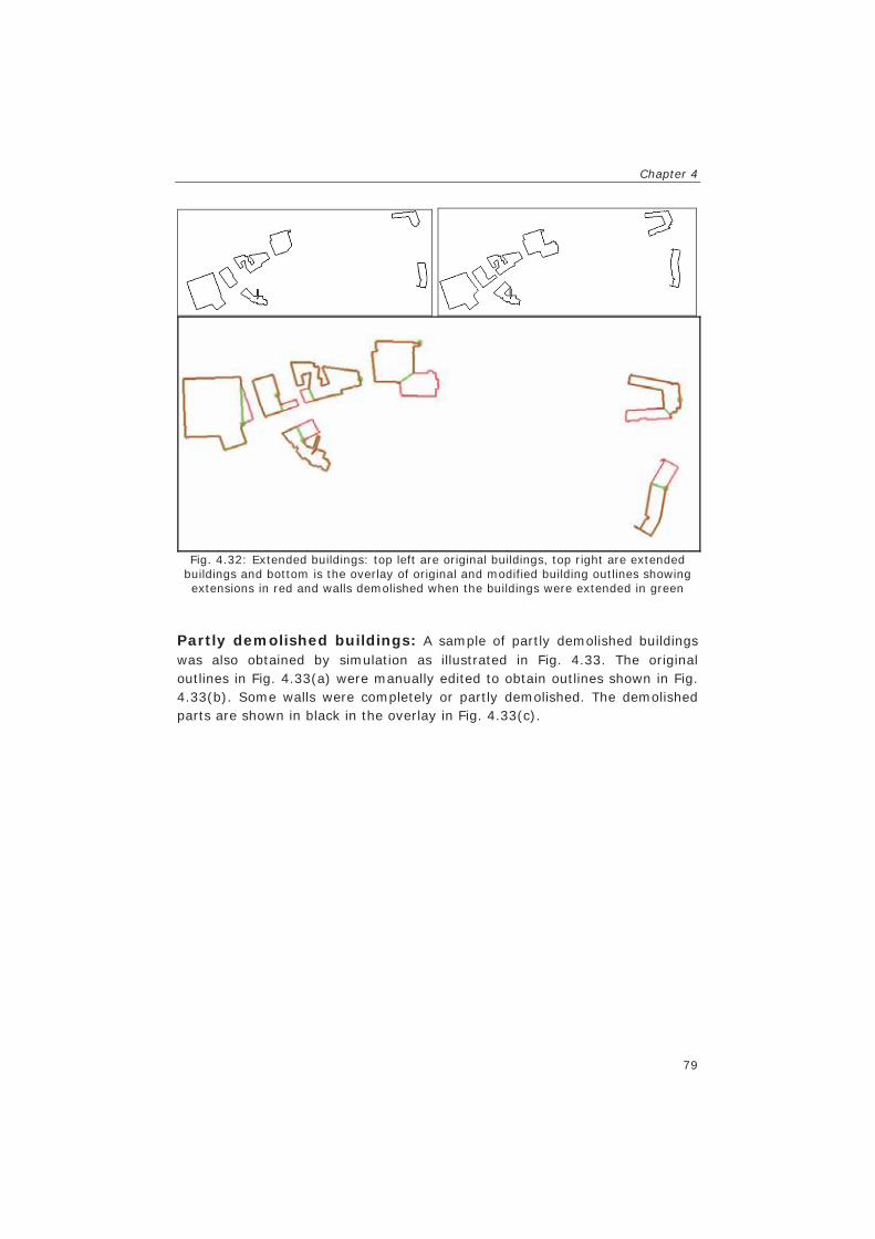
Chapter 4
79
Fig. 4.32: Extended buildings: top left are original buildings, top right are extended
buildings and bottom is the overlay of original and modified building outlines showing extensions in red and walls demolished when the buildings were extended in green
Partly demolished buildings: A sample of partly demolished buildings was also obtained by simulation as illustrated in Fig. 4.33. The original outlines in Fig. 4.33(a) were manually edited to obtain outlines shown in Fig. 4.33(b). Some walls were completely or partly demolished. The demolished parts are shown in black in the overlay in Fig. 4.33(c).

Experimental verification of 2D building outlines
80
Fig. 4.33: Partly demolished buildings: a) original buildings b) partly demolished c) overlay showing black parts as demolished walls. The black walls are identified as
demolished when they are completely demolished (See Fig. 4.34) Verification results at per-wall level for the case of AdaBoost are shown in Fig. 4.34. For most walls the demolished walls could be distinguished from existing ones. The results for demolished walls were generally closer to 0 while for unchanged walls the results were closer to 1. There were also some walls that were partly demolished. The results for these walls were arbitrary (some memberships close to 0 and others close to 1).

Chapter 4
81
00.10.20.30.40.50.60.70.80.9
1
0 20 40 60 80 100 120 140 160 180Wall#
Mem
bers
hip
to e
xist
s
Demolished walls Partly demolished walls Not modified walls
Fig. 4.34: Verification results for walls of partly demolished buildings
At per-building level, all modified buildings were identified (Table 4.15). In general, these experiments have shown that modified buildings are inferred when some of the walls of a building are verified as existing while others are identified as demolished.
Table 4.15: Building verification results with Haiti buildings and Pictometry images
Reference Modified buildings
AdaBoost RTrees Hints
Unchanged% 0 0 0
Demolished% 0 0 0
Modified % 100 100 100
4.7 Transferability of training data If training done for one area or by using one type of dataset gives good results when experiments are conducted over other areas or by using other datasets, then the efforts required for training are reduced. Therefore, it is interesting to check if the training done by using one image dataset can be useful for verification by using other image datasets. It is also interesting to test if training with buildings from one area (one city) can be useful for verification of buildings in another area. For some buildings in the Enschede data experiments were conducted by using different images for training and verification. The training was done by using AdaBoost classifier. In the first instance training was done by using Pictometry images followed by verification using Slagboom en Peeters images

Experimental verification of 2D building outlines
82
and the second instance the training was done by using Slagboom en Peeters images followed by verification using Pictometry images. The results are shown in Table 4.16 for completeness and Table 4.17 for correctness. Although the majority of walls are correctly classified as existing or demolished, these results are significantly lower than those obtained by training and verification with the same images (as discussed in Section 4.5).
Table 4.16: Wall verification results (completeness) obtained from training with different images
Images used for Training /verification
Completeness_Existing
Completeness_Demolished
Pictometry/ Slagboom en Peeters 88% 57% Slagboom en Peeters/ Pictometry 77% 70%
Table 4.17: Wall verification results (correctness) obtained from training with different
images Images used for
Training /verification Correctness_
Existing Correctness_ Demolished
Pictometry/ Slagboom en Peeters 73% 78% Slagboom en Peeters/ Pictometry 79% 67%
In a similar manner, by using Enschede buildings and Pictometry images, verification experiments were done for Haiti data using Haiti Pictometry images. The results are shown in Fig. 4.35 for existing walls and Fig. 4.36 for demolished walls. The results show weak categorisation of existing buildings. This could be due to the differences of buildings in Haiti and Enschede. Some features which are strong for verification of buildings in one area (such as Enschede in Netherlands) are weak for another part of the world (Port-au-Prince in Haiti). In this case it cannot be concluded that training done in one area can be used for another area.
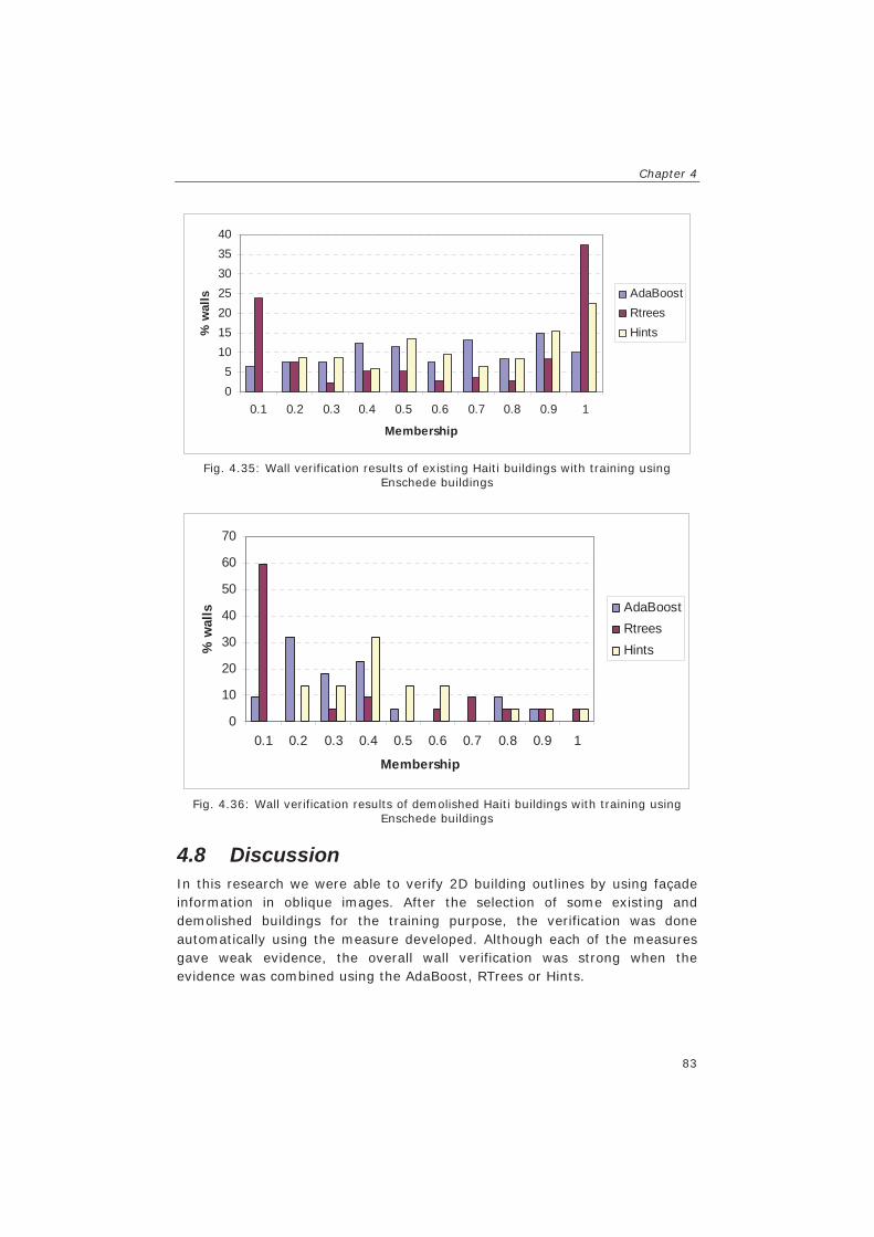
Chapter 4
83
05
10152025303540
0.1 0.2 0.3 0.4 0.5 0.6 0.7 0.8 0.9 1
Membership
% w
alls AdaBoost
RtreesHints
Fig. 4.35: Wall verification results of existing Haiti buildings with training using
Enschede buildings
0
10
20
30
40
50
60
70
0.1 0.2 0.3 0.4 0.5 0.6 0.7 0.8 0.9 1
Membership
% w
alls AdaBoostRtreesHints
Fig. 4.36: Wall verification results of demolished Haiti buildings with training using
Enschede buildings
4.8 Discussion In this research we were able to verify 2D building outlines by using façade information in oblique images. After the selection of some existing and demolished buildings for the training purpose, the verification was done automatically using the measure developed. Although each of the measures gave weak evidence, the overall wall verification was strong when the evidence was combined using the AdaBoost, RTrees or Hints.
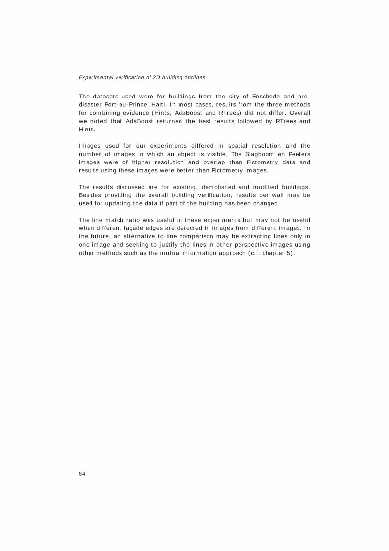
Experimental verification of 2D building outlines
84
The datasets used were for buildings from the city of Enschede and pre-disaster Port-au-Prince, Haiti. In most cases, results from the three methods for combining evidence (Hints, AdaBoost and RTrees) did not differ. Overall we noted that AdaBoost returned the best results followed by RTrees and Hints. Images used for our experiments differed in spatial resolution and the number of images in which an object is visible. The Slagboom en Peeters images were of higher resolution and overlap than Pictometry data and results using these images were better than Pictometry images. The results discussed are for existing, demolished and modified buildings. Besides providing the overall building verification, results per wall may be used for updating the data if part of the building has been changed. The line match ratio was useful in these experiments but may not be useful when different façade edges are detected in images from different images. In the future, an alternative to line comparison may be extracting lines only in one image and seeking to justify the lines in other perspective images using other methods such as the mutual information approach (c.f. chapter 5).

85
5. Verification of 3D building models using oblique airborne images2
This chapter describes a method for automatic verification of 3D building models using airborne oblique images. The problem being tackled is identifying buildings that are demolished or changed since the models were constructed or identifying wrongly constructed models using the images. The models verified are of CityGML level of detail 2 (LOD2) or higher since their edges are expected to coincide with actual building edges. Chapters 3 and 4 of this thesis were dedicated to verification of 2D building datasets. In that case, wall faces used for the verification, were not explicit and the hypotheses to be verified entailed generation of rough estimates of heights of buildings and the ground. For the 3D case, the method takes wall and roof structures (roof edges, roof faces and wall faces) of the model as input. As opposed to the 2D case, here also the roof plays a major role. The result of combining roof and wall information is expected to be better than when using walls or roofs alone. The use of roof in addition to wall information is possible because the whole structure of a building (walls and roofs) are available in oblique images. Roof views are large both in nadir and oblique images. However, we expect roof verification results from oblique images to be better because of the tilted view where height changes are more obvious and should be detected more reliably. In Section 2.1 the state of the art verification of buildings was discussed. Image-based methods proposed for verification of 3D building models include classification involving training with roof colours and texture comparison of multi-view or multi-temporal images. In the former case (using colour classification), confusion happens for roads or other surfaces with colours similar to buildings and in the latter (using multiple image comparison), problems may happen particularly for roofs if objects such as dormer windows protrude on the subject surfaces.
5.1 The approach Our verification approach is based on information theory. Corresponding variables between edges of building models and oblique images are used for
2 This chapter includes contents from Nyaruhuma et al. (2012)

Verification of 3D building models using oblique airborne images
86
deriving mutual information. The mutual information combined for all perspective images available is used for the verification. The concept of mutual information was first introduced by Shannon (1948) for optimising information transfer in communication channels with disturbances between the source and the receiver. Mutual information has been used for many applications as a way of modelling uncertainty between related variables. For example, Vosselman (1992) used mutual information for relational matching and Suveg and Vosselman (2002) developed a method for modelling mutual information between 3D building model contours and image pixel gradient magnitude and used the method for evaluating building models constructed using aerial images and maps (Suveg and Vosselman, 2004). Our model verification method includes the following aspects. Firstly, it uses oblique images and therefore we have substantial view of walls of buildings in addition to roofs. Secondly, the images used are captured with multiple overlap and from very different perspectives which allows for better identification of imaged objects. Thirdly, new variables are proposed for obtaining mutual information. Some of the already proposed methods use the correspondence of lines extracted in images to edges of building models (Huertas and Nevatia, 2000; Lowe, 1987). The results in this case depend on the quality of line extraction. In this research the wireframe model edges are projected to images and verified using low level image features. We propose a variant to the procedure by Suveg and Vosselman. Instead of pixel gradient magnitude, we propose the use of gradient direction. Fourthly, we do visibility analysis so as to concentrate only on roof edges that are not occluded by other objects. Lastly, we statistically find out the minimum amount of mutual information required for our verification purpose. The following assumptions are considered. The building models verified are expected to be detailed and not generalised (CityGML LOD2 and above). Fig. 5.1 shows a sample of the models verified. The images are also expected to be of high spatial resolution where edges of the buildings can be observed. Fig. 5.2 is a sample of the image.
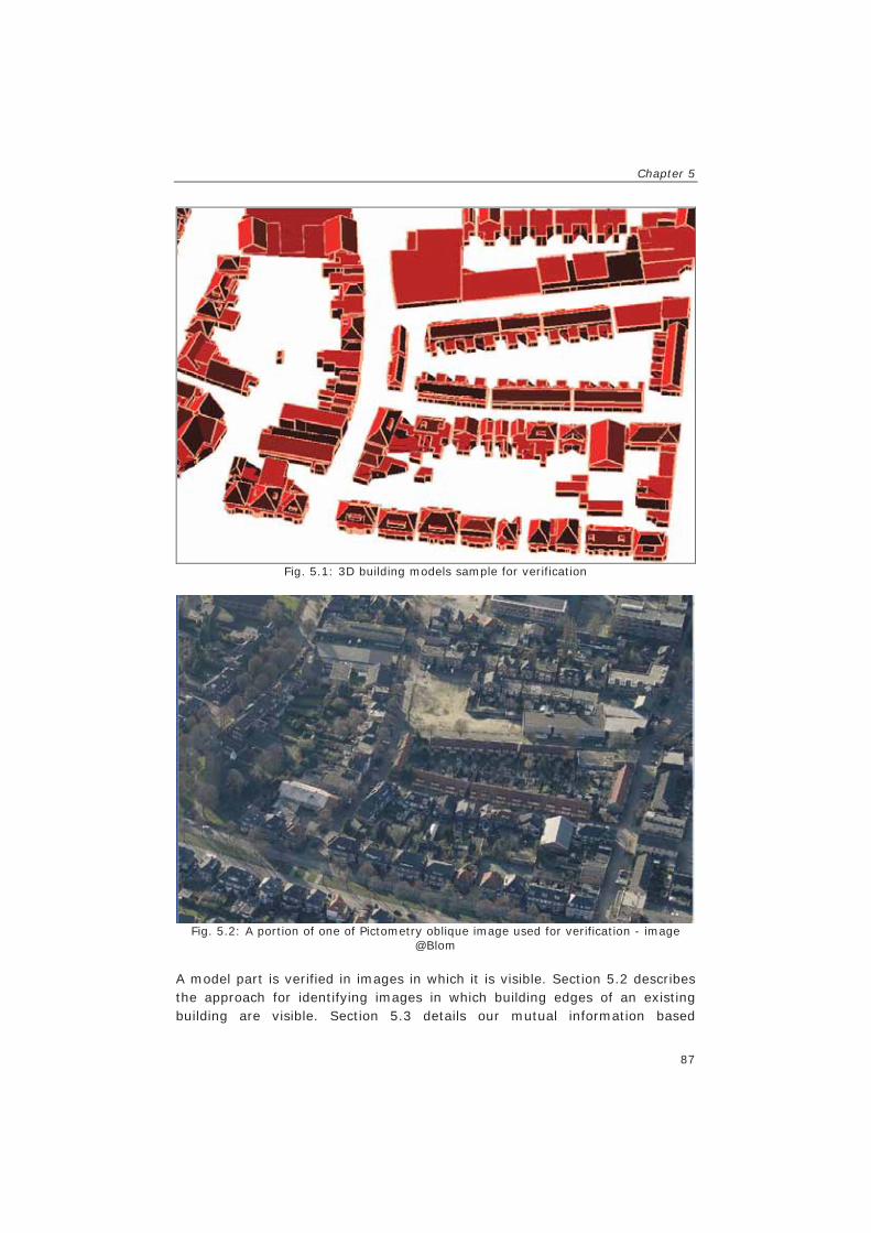
Chapter 5
87
Fig. 5.1: 3D building models sample for verification
Fig. 5.2: A portion of one of Pictometry oblique image used for verification - image
@Blom A model part is verified in images in which it is visible. Section 5.2 describes the approach for identifying images in which building edges of an existing building are visible. Section 5.3 details our mutual information based

Verification of 3D building models using oblique airborne images
88
approach to building verification. The mutual information approach is used for verification of roofs. The verification of walls is discussed in Section 5.4.
5.2 Visibility analysis An important step in the verification method is to determine if an edge of a building is imaged given camera position and other objects that are in the scene and may be occluding the building. The visibility analysis is done in two steps. The first step considers only orientation of the model faces relative to the camera. Edges of surfaces that are not facing the camera are identified and eliminated. The second step checks if an edge is occluded by other objects such as other faces of the same building, other buildings or trees. For this purpose we use a point cloud obtained from dense matching (Furukawa and Ponce, 2010) in the oblique images. Although the existing models could be used as well to check whether buildings occlude others, by employing the point cloud we are independent from possible errors in the model. We also detect occlusion by other objects such as trees. Visibility analysis for wall faces was described in Section 3.2. We have developed a similar approach for analysing visibility of individual roof edges.
B
P
A
B
P
A
Fig. 5.3: The edge defined by line AB is occluded because the points on the large
building are above the plane ABP Edge visibility analysis is illustrated in Fig. 5.3. The camera position is P and the model edge being tested for visibility is AB. The visibility analysis is done by testing the presence or absence of objects obstructing rays from the camera to the edge. By using the point cloud, we first isolate all points that belong to connected components and are in between the camera and a buffer around the edge. The connected components are composed by constraining on a maximum distance between points and a minimum number of points for a component.
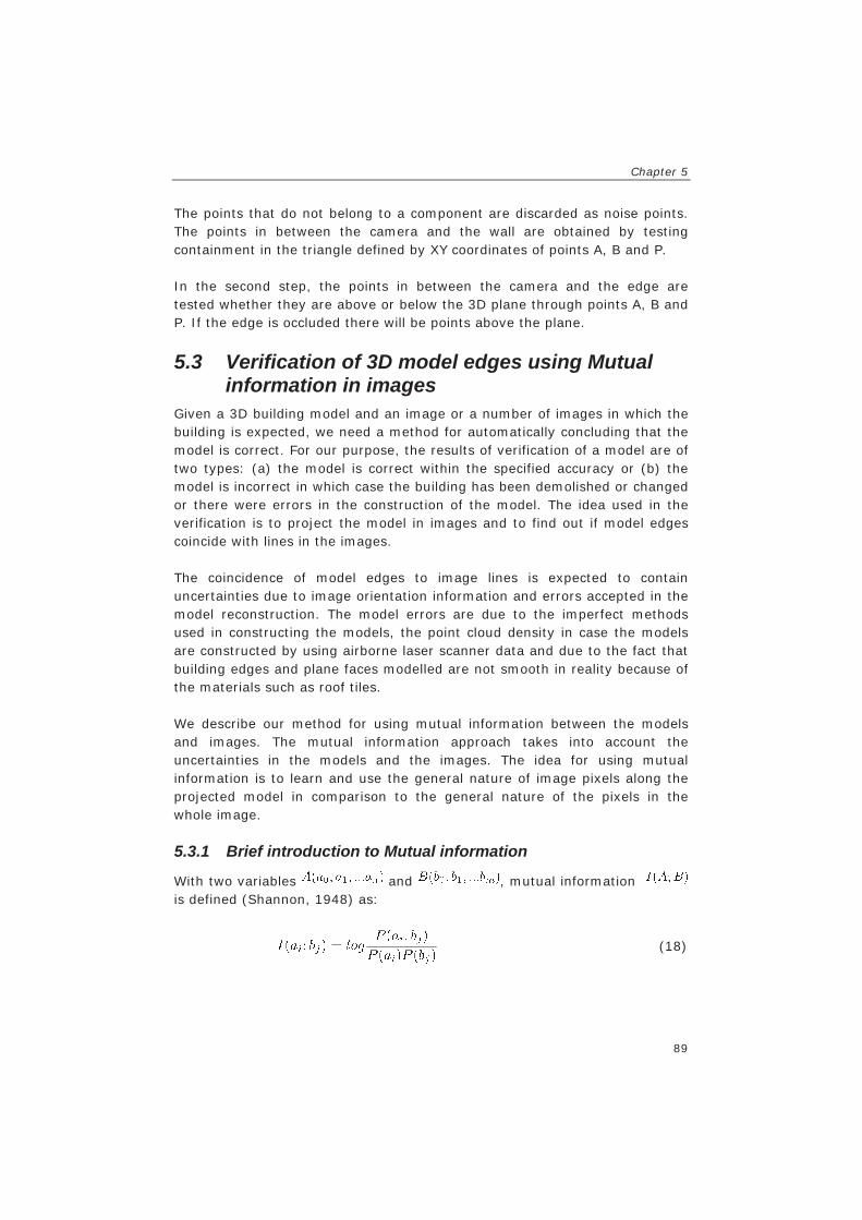
Chapter 5
89
The points that do not belong to a component are discarded as noise points. The points in between the camera and the wall are obtained by testing containment in the triangle defined by XY coordinates of points A, B and P. In the second step, the points in between the camera and the edge are tested whether they are above or below the 3D plane through points A, B and P. If the edge is occluded there will be points above the plane.
5.3 Verification of 3D model edges using Mutual information in images
Given a 3D building model and an image or a number of images in which the building is expected, we need a method for automatically concluding that the model is correct. For our purpose, the results of verification of a model are of two types: (a) the model is correct within the specified accuracy or (b) the model is incorrect in which case the building has been demolished or changed or there were errors in the construction of the model. The idea used in the verification is to project the model in images and to find out if model edges coincide with lines in the images. The coincidence of model edges to image lines is expected to contain uncertainties due to image orientation information and errors accepted in the model reconstruction. The model errors are due to the imperfect methods used in constructing the models, the point cloud density in case the models are constructed by using airborne laser scanner data and due to the fact that building edges and plane faces modelled are not smooth in reality because of the materials such as roof tiles. We describe our method for using mutual information between the models and images. The mutual information approach takes into account the uncertainties in the models and the images. The idea for using mutual information is to learn and use the general nature of image pixels along the projected model in comparison to the general nature of the pixels in the whole image.
5.3.1 Brief introduction to Mutual information
With two variables and , mutual information is defined (Shannon, 1948) as:
(18)

Verification of 3D building models using oblique airborne images
90
In this equation is the joint probability and and are marginal probabilities. Mutual information can also be computed by substituting from the conditional probability concept:
(19)
The mutual information is then
(20)
In this case, mutual information is the difference between self-information
and conditional information : (21) Where and The self-information gives the amount of information about a variable irrespective of the other variable and the conditional information models the dependency of the two variables. When the self-information and conditional information are the same, the mutual information is 0. This happens when the variables are independent. Higher differences between conditional information and self-information results to mutual information much above zero or much below zero. Because of the ability to handle uncertainties, mutual information has been used for many applications, including the original analysis of information sent over noisy channels and computation of collocations (sequences of words that occur together more often than would be expected by chance). In our case, image pixels are used to obtain information about building models. Using mutual information we identify a correct model edge in the presence of some random noise pixels that do not support the existence of the edge. We use Equation (20) for obtaining mutual information between 3D models and images. We model image features that give evidence for the presence of
a building into the two probability densities and . The probability density is obtained by using image information for the variable at
Chapter 5
91
random positions while is obtained for image positions with the model edges. Features used are discussed below.
5.3.2 Mutual information using model edges This part describes the procedure for obtaining mutual information between images and building models. We use image pixel gradients from the Sobel operator but, instead of gradient magnitude, we use the gradient direction. The reasons for this choice are discussed in Section 5.3.3 below. Pixel gradient direction probability density: To obtain mutual information using model edges we first estimate the pixel gradient direction probability density and edge pixel gradient direction (conditional) probability density as follows. Some model edges (such as 500 in total) used for training are projected into images and the direction of each of the projected edge is computed. From the images we also compute gradient directions
for pixels a) chosen at random image positions and b) along the projected edges. Intuitively, gradient directions computed for pixels at random image positions are equivalent to gradient directions for pixels along random edge segments placed in the image. Using the gradient directions we compute two sets of angles and their distributions. The first is a set of angles each between a random pixel gradient direction and the direction of a projected model edge chosen
randomly. The second is a set of angles each between the gradient direction of a pixel along an image line obtained by projecting a model edge and the direction of the line. Each angle is computed as:
(22)
For each of the two sets, we make a histogram with classes of angles such as 1 degree (180 classes) and assign every angle a class in order to obtain a distribution of the angles. The two distributions are the pixel gradient
direction probability density and the edge pixel gradient direction probability density . From pixel direction probability density and edge pixel direction probability density we compute mutual information for each of the angles as:
(23)
Examples of pixel gradient direction probability density and edge pixel direction (conditional) probability density are shown in Fig. 5.4 for Pictometry

Verification of 3D building models using oblique airborne images
92
images and Fig. 5.5 for Slagboom en Peeters images. In both figures, the two densities reveal the following aspects.
0
0.005
0.01
0.015
0.02
0.025
0 30 60 90 120 150 180
angle
prob
abili
ty
p( j) p( j|L)
Fig. 5.4: Pixel gradient direction probability density and the edge pixel gradient direction probability density obtained by using Pictometry images
0
0.01
0.02
0.03
0.04
0.05
0.06
0 20 40 60 80 100 120 140 160 180
angle
prob
abili
ty
p( j) p( j|L)
Fig. 5.5: Pixel gradient direction probability density and the edge pixel gradient direction probability density obtained by using Slagboom en Peeters images
Firstly, we note the uniform distribution of the pixel gradient direction signified by near linear (horizontal) blue lines in the figures. This is as expected because pixels randomly selected from a scene containing buildings, roads, trees etc. should have gradients facing all directions. Secondly, the highest probability of the edge pixel directions is around 90 degrees. This is also as expected because pixel gradient directions along an edge are ideally in normal direction to the edge. The distribution exhibits the

Chapter 5
93
characteristics of the von Mises distribution with standard deviation depending on the signal to noise ratio and the uncertainties in the model edges. Thirdly, the pixel gradient direction probability curve and edge pixel gradient direction probability reveal a clear difference (with a large area between them) which is an important element for mutual information. To further compare the probability distributions obtained with Pictometry and Slagboom en Peeters images, the pixel gradient direction probability curve from the two images types were plotted jointly as shown in Fig. 5.6 and edge pixel gradient direction probability curves for the two image types were plotted together as shown in Fig. 5.7. The two curves in Fig. 5.6 are very similar implying the self information is the same in both images. This is as expected because pixel gradients, of typical scene captured in an airborne image, are normally point in random directions.
0
0.01
0.02
0.03
0.04
0.05
0.06
0 30 60 90 120 150 180
angle
prob
abili
ty
Slagboom en Peeters images p( j|L) Pictometry p( j|L)
Fig. 5.6: Pixel gradient direction probability density obtained from Pictometry and Slagboom en Peeters images compared

Verification of 3D building models using oblique airborne images
94
0
0.01
0.02
0.03
0.04
0.05
0.06
0 30 60 90 120 150 180
angle
prob
abili
ty
Slagboom en Peeters images p( j|L) Pictometry p( j|L)
Fig. 5.7: Edge pixel gradient direction probability density obtained from Pictometry and Slagboom en Peeters images compared
For the case in Fig. 5.7 the curve obtained from Slagboom en Peeters images is smoother and has a sharper peak than the one obtained with Pictometry images. This is because structures are better visible in Slagboom en Peeters images due to higher resolution and therefore there is less uncertainty in gradients of pixels along model edges. It implies that edges can be recognised better in Slagboom en Peeters than Pictometry images. The distributions in the two figures (Fig. 5.6 and Fig. 5.7), similar for the former and different for the latter, also imply that the determinant of the difference in mutual information between two images types does not depend on the pixel gradient direction probability density but the edge pixel gradient direction probability density. This implies that when training with a new image type, concentration should be on edge pixel gradient direction probability density and not the pixel gradient direction probability density. The mutual information: The mutual information from the densities on Fig. 5.4 (Pictometry) and Fig. 5.5 (Slagboom en Peeters) is shown jointly in Fig. 5.8. The total mutual information for either of the curves is the sum of the area under the curve (positive mutual information) and the area over the curve (negative mutual information). From the figure, the area is for Slagboom en Peeters is larger than for Pictometry indicating that the amount of mutual information for Slagboom en Peeters is more than for Pictometry.

Chapter 5
95
-5-4-3
-2-101
234
0 30 60 90 120 150 180
angle
mut
ual i
nfo.
(I)
Slagboom en Peeters Pictometry
Fig. 5.8: Mutual information for different angles between projected model edges and pixel gradient directions
For each pixel on the edge being verified we compute the amount of mutual information. In Section 5.3.4 we describe the combination of mutual information from different pixels and discuss the procedure for setting the minimum amount of mutual information required for categorising a model edge as existing in the image.
5.3.3 Robustness of the gradient directions with respect to illumination change
For our purpose, gradient directions are preferred over gradient magnitude. The main reason is that the gradient magnitude differs with change of illumination while the directions are not affected. The other reason for not using gradient magnitude for edge verification is that the magnitude may be higher irrespective of direction. Example cases are when an edge being verified does not exist in the image but its position intersects other edges facing different directions. The pixels on this intersection will have high gradient magnitude. For comparison purposes, gradient magnitudes were also used to generate graphs similar to Fig. 5.4 trough Fig. 5.8. The graphs in Fig. 5.9 are probability densities obtained with Pictometry images by using the pixel gradient magnitudes instead of the angles and Fig. 5.10 shows the corresponding mutual information. From Fig. 5.9, we noted that for many gradients, the edge pixel gradient probability density was uniform. We also noted that mutual information was zero (at the intersection of the two curves) when the edge pixel gradient probability was close to maximum. This implies that there are many edge

Verification of 3D building models using oblique airborne images
96
pixels for which there is no information obtainable from pixel gradient magnitudes.
0
0.005
0.01
0.015
0.02
0 200 400 600 800 1000
pixel gradient
prob
abili
ty
p(Gj) p(Gj|L)
Fig. 5.9: Probability density obtained by using pixel gradient magnitude instead of gradient directions - for pixel gradient probability density and for edge
pixel gradient probability density
-8
-6
-4
-2
0
2
4
6
8
0 200 400 600 800 1000
pixel gradient
mut
ual i
nfor
mat
ion
(I)
Fig. 5.10: Mutual information for different gradient magnitudes obtained by using
pixels on projected model edges and random pixels
5.3.4 Verification using mutual information Combining information: Using the method described in Section 5.3.2 we compute mutual information for all pixels along an edge projected to an image. We assume that image pixels are independent and compute mutual information for a whole model edge as a sum for all pixels along the edge.
Chapter 5
97
The mutual information computation is summed for pixels in all the three RGB channels of the image. We also assume independence of pixels from image taken from different perspectives. Even when an edge of a demolished building model coincides with an arbitrary line in the image, the wrong result is suppressed by the absence of the same line in images from other perspectives. Thus, the sum is also computed over all images in which a model edge may be visible. Thus the mutual information for a model edge
is obtained as (24)
The verification results are therefore obtained per edge. For purposes such as model improvement and refinement this may be the required result. Individual edges which are verified as incorrect or demolished will be checked by the operator for capturing the changes. Results may also be combined per model face or the whole model. A simple way is to obtain the sum of mutual
information for all the edges of the face or the model computed as in equation (25). Some operations may also be used in improving and edge verification results by taking into account context information such as the status of edges sharing nodes. (25)
Data uncertainty consideration: Mutual information is computed taking into consideration uncertainties in model edge position and image orientation. Edge pixel gradient directions are computed not only along the projected edge but also for some lines constructed - at one pixel distance each - within a buffer of the projected edge. The buffer is determined by taking into account the uncertainties in the image orientation and the model construction. Then the mutual information of the line with the maximum mutual information among the lines in the buffer is selected. Determination of sufficient mutual information: For categorising a model edge as correct we use a statistical test on the amount of mutual information that is sufficient within a confidence limit (Vosselman, 1992, p. 138-141). Consider the mutual information shown in Fig. 5.8 and the edge pixel gradient direction probability density shown in Fig. 5.4. By combining
the function in Fig. 5.4 and in Fig. 5.8 one can calculate the
probability that a certain amount of mutual information will be found for an edge pixel:

Verification of 3D building models using oblique airborne images
98
(26)
From this, one can derive the probability that the mutual information will be within a certain range .
(27)
Equation (27) is for a continuous case but in our case the distribution is discrete and thus the probability for the range of mutual information is: (28)
Using equation (28) the required minimum mutual information for classifying a pixel as being on an existing model edge is obtained by considering a threshold based on an acceptable type I error such as 0.05 (i.e.
). That is, we seek which satisfies the equation:
(29)
For practical computation of the threshold we use the cumulative distribution of mutual information. Using Pictometry images, for one pixel the cumulative distribution is as shown in Fig. 5.11 and for different numbers of edge pixels, we obtain different computed distributions. A combination of more pixels results to less negative mutual information and the 0.05 threshold should be at more bits. A building model with 400 pixels (for all edges in all images) will be accepted as correct with 95% confidence if the aggregate mutual information is above 633 bits (Fig. 5.12). For each model, an individual threshold for its acceptance will be computed according to the number of pixels for all edges and for all images where it is visible. For computational reasons, a look-up table is obtained beforehand.

Chapter 5
99
00.10.20.30.40.50.60.70.80.9
1
-2.5 -2 -1.5 -1 -0.5 0 0.5 1 1.5 2 2.5
I(bits)
cum
m. p
rob.
Fig. 5.11: Mutual information cumulative distribution for one pixel – the arrow indicates
the 0.05 threshold (95% confidence)
0.0
0.1
0.2
0.3
0.4
0.5
0.6
0.7
0.8
0.9
1.0
600 650 700 750
I (bits)
cum
m. p
rob.
400 pixels
Fig. 5.12: Mutual information distribution for 400 pixels
5.4 Combining wall and roof verification results Building models include roof and wall faces. In order to obtain the overall status of a building, verification is done by using evidence from both walls and roofs. Roofs are verified by using model edges and the mutual information approach described in the preceding sections and, the walls are verified by using façade measures (Line Match Ratio, Line Direction Ratio, etc) discussed in Chapter 3. Roof and wall verification results can be used for identifying the status of a building. When roof edges and wall faces have been verified independently, some rules can be used to make combined inference. For example, if roof edges of a building model do not coincide with image line segments, the mutual information approach will indicate that the model edges are incorrect. If at the same time walls of this building are verified as

Verification of 3D building models using oblique airborne images
100
existing in the images, then the interpretation can be that the building has been extended vertically. When a building is extended vertically, walls of the building in the old state are still correct but the roof edges are not. Another case is when roof edges of a building model coincide with image line segments indicating that the model edges are correct. If at the same time walls are verified as demolished in the images, then the interpretation can be that the wall results are due to errors in the verification as it is not possible for a roof to exist when walls are demolished. Using the same line of thinking, rules shown in Table 5.1 can be applied specifically.
Table 5.1: Building status inferred from roof and wall verification results Roof results Wall results Inference Roof verified as correct
Walls verified as correct
Building not changed
Roof verified as correct
Walls verified as incorrect
Building not changed (i.e. erroneous wall result)
Roof verified as correct
Walls verified as undecided
Building not changed (decision based on roof only)
Roof verified as incorrect
walls verified as correct
Building modified vertically or roof model incorrect
Roof verified as incorrect
walls verified as incorrect
Building demolished or model incorrect
Roof verified as incorrect
walls verified as undecided
Building demolished (decision based on roof only)
The combination of roof and wall information is expected to give building verification results that are better than those obtained with walls or roofs alone. These kind of analyses are also favoured by the availability of the whole structure of a building (walls and roofs) in oblique images.

101
6. Experimental verification of 3D building models
6.1 Experimental design The purpose of experiments discussed in this chapter is to evaluate the method developed for verification of 3D building models. To achieve this, we used sample datasets of building models and oblique images. The building models represent the old situation and the oblique images represent the current situation to which the building models are compared against. Several issues were investigated. Firstly, we intended to find out the completeness and correctness that can be achieved by using the method developed. For this purpose, we conducted experiments with models of actually existing and demolished buildings and analysed their results. Secondly, since roof faces used in our verification are also available in vertical views, we intention to find out how the method works for nadir images. We therefore conducted verification experiments by using nadir looking images and compared the results with those obtained from oblique images. We expected results from oblique images to be better because of the tilted view where height changes are more obvious and should be detected more reliably. Thirdly, we intended to identify the benefit of using image datasets with higher overlap and higher spatial resolution. For this purpose, we conducted experiments using two image datasets with different overlap and resolution. Lastly, since images contain information on both walls and roofs of buildings, we expected better verification results when all this information is used. We therefore compared, per building, the results from roof, walls and the combination of roof and walls. In order to analyse the performance of the developed approach we needed to conduct experiments with large samples. Thus, many demolished buildings were obtained by simulation in this research. The simulation was done by shifting building models of existing buildings to other arbitrary places. Mutual information training was done as discussed in Section 5.3.2. Initially, the training was done by using a sample of edges from the building models. Because it was noticed in our training experiments that edges randomly extracted in images produced edge pixel gradient direction probability densities similar to those obtained with edges of actual models projected on
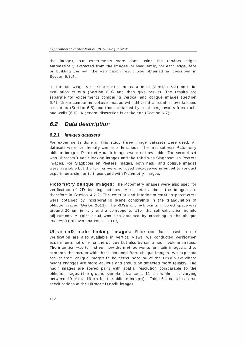
Experimental verification of 3D building models
102
the images, our experiments were done using the random edges automatically extracted from the images. Subsequently, for each edge, face or building verified, the verification result was obtained as described in Section 5.3.4. In the following, we first describe the data used (Section 6.2) and the evaluation criteria (Section 6.3) and then give results. The results are separate for experiments comparing vertical and oblique images (Section 6.4), those comparing oblique images with different amount of overlap and resolution (Section 6.5) and those obtained by combining results from roofs and walls (6.6). A general discussion is at the end (Section 6.7).
6.2 Data description
6.2.1 Images datasets For experiments done in this study three image datasets were used. All datasets were for the city centre of Enschede. The first set was Pictometry oblique images. Pictometry nadir images were not available. The second set was UltracamD nadir looking images and the third was Slagboom en Peeters images. For Slagboom en Peeters images, both nadir and oblique images were available but the former were not used because we intended to conduct experiments similar to those done with Pictometry images. Pictometry oblique images: The Pictometry images were also used for verification of 2D building outlines. More details about the images are therefore in Section 4.2.2. The exterior and interior orientation parameters were obtained by incorporating scene constraints in the triangulation of oblique images (Gerke, 2011). The RMSE at check points in object space was around 20 cm in x, y and z components after the self-calibration bundle adjustment. A point cloud was also obtained by matching in the oblique images (Furukawa and Ponce, 2010). UltracamD nadir looking images: Since roof faces used in our verification are also available in vertical views, we conducted verification experiments not only for the oblique but also by using nadir looking images. The intention was to find out how the method works for nadir images and to compare the results with those obtained from oblique images. We expected results from oblique images to be better because of the tilted view where height changes are more obvious and should be detected more reliably. The nadir images are stereo pairs with spatial resolution comparable to the oblique images (the ground sample distance is 11 cm while it is varying between 10 cm to 16 cm for the oblique images). Table 6.1 contains some specifications of the UltracamD nadir images.

Chapter 6
103
Table 6.1: Specifications of the nadir images from UltracamD Parameter Value Flying height (m) 1200 Baseline(m) 800 Focal length of camera (mm) 101 Pixel size ( m) 9 Ground sample distance -GSD (cm) 11
A portion of one of the Pictometry images is shown in Fig. 6.1 (left), a corresponding portion from the UltracamD nadir images is shown in Fig. 6.1 (middle) and a portion of the point cloud overlaid with building models is shown in Fig. 6.1 (right).
Fig. 6.1: The same roof in an oblique image ©Blom of the city centre of Enschede, a
nadir looking image from UltracamD and a point cloud (coloured according to elevation) obtained from oblique images overlaid with 3D models
Slagboom en Peeters oblique images: The other dataset of oblique images used is from Slagboom en Peeters Luchtfotografie BV. The images were taken with more overlap and higher spatial resolution than Pictometry. More details about the images are also in Section 4.2.2. For purpose of roof comparison, two patches obtained by zooming into Pictometry and Slagboom en Peeters are shown in Fig. 6.2.

Experimental verification of 3D building models
104
Fig. 6.2: The same roof in Pictometry (left) and Slagboom en Peeters (right) images
6.2.2 Buildings verified For this study we used 3D building models for a part of the city of Enschede in the Netherlands. The model construction was not part of this work. The models were already constructed using a target based graph matching approach (Oude Elberink and Vosselman, 2009). Fig. 6.3 shows a sample of models verified. The results obtained with these models were used for comparison of oblique and vertical images as discussed in Section 6.4. Another sample is shown in Fig. 6.4. It was used for comparison of results from images with different spatial resolution and overlap (Pictometry and Slagboom en Peeters), discussed in Section 6.5. The developed verification method takes into account uncertainties in the model and in the image orientation parameters. A detailed analysis of the quality of model construction was discussed in (Oude Elberink and Vosselman, 2011), where the total standard deviation was estimated at around 25 cm in x, y and z components. In our verification procedure we would like to capture modelling errors caused by data gaps and the difficulty of ascertaining roof outlines using laser point clouds. We therefore assume a lower standard deviation of 10 cm. By using a sample of model edges manually identified as correct and projected in images we have estimated the standard deviation of the position of the edges in images at around 0.5 pixels of Pictometry and Ultracam images and 1 pixel of Slagboom en Peeters images. For our experiments, we have therefore used one pixel (2 times 0.5) as the tolerance with 95% confidence for Pictometry and UltracamD and two pixels for Slagboom en

Chapter 6
105
Peeters images. Pixels within the buffer defined this way are used for computing gradients used for verification.
Fig. 6.3: One sample of 3D building models used for verification experiments
Fig. 6.4: Another sample of 3D building models used for verification experiments
6.3 Evaluation criteria The null-hypothesis constructed for every model edge (also per face or building) is “the edge exists”. From experiments, correct and wrong verification results are obtained and then the completeness and correctness percentages are computed in the manner described for evaluating results of verification of 2D building outlines (Section 4.4).

Experimental verification of 3D building models
106
Similar to the evaluation of the verification of walls, the Completeness_Exists is the proportion of correctly verified roof faces among all existing faces in the sample and the Completeness_Demolished is the proportion of demolished roof faces identified among all demolished roof faces in the sample. The Correctness_Exists is the number of roof faces correctly verified among all roof faces categorised as existing and Correctness_Demolished is the number of demolished roof faces correctly identified among all roof faces identified as demolished.
6.4 Results from oblique and vertical images The following are results obtained by using our method to verify existing and demolished buildings (i.e. correct and wrong models) by using oblique (Pictometry) and vertical (UltracamD) images. The results for individual edges are combined per roof face and per building model as discussed in 5.3.4. The experiments were done for 98 existing and 114 demolished buildings in oblique images and 94 existing and 118 demolished buildings in vertical images. The two image types were not taken at the same period and some buildings were changed (actually 4 were demolished) in between. The numbers for all the edges, roof faces and buildings are shown in Table 6.2.
Table 6.2: The number of edges, faces and buildings verified in Oblique and vertical images
Image type exists demolished
Edges Oblique 1413 1709
Vertical 1292 2063
Roof faces Oblique 450 586
Vertical 411 609
Buildings Oblique 98 114
Vertical 94 118
The results for the actual buildings are shown in Fig. 6.5. In the figure, the results using oblique images are to the left and those obtained with nadir images are to the right. From top to the bottom, the results are per edge (top), per roof face (middle) and per building (bottom). The lines shown in green were identified as existing (or correct model), the red were identified as demolished (or wrong model) and the yellow represent the incorrect model lines that were identified as correct in vertical images. The yellow lines were wrongly identified as correct mainly because some automatically reconstructed flat roof models had correct building footprints but a wrong
Chapter 6
107
height. This results to only a small difference in image position relative to the position of the real roof location. As can be noted, there are fewer red lines at per roof face level than at per edge level. This is a result of aggregating mutual information for all edges of a face. Similarly, there are fewer red lines at per building level than at per roof face level. It can also be noted that the buildings that were demolished in between the periods of capture of the oblique and nadir images were correctly identified. Looking at the bottom right image, the red lines in the middle of the image represent a building that was demolished during this period. The corresponding lines in the left image are correctly in green. For the simulated buildings the results are shown in Fig. 6.6. As can be noted, nearly all lines are red, indicating that they were correctly identified as demolished (or models were wrong).
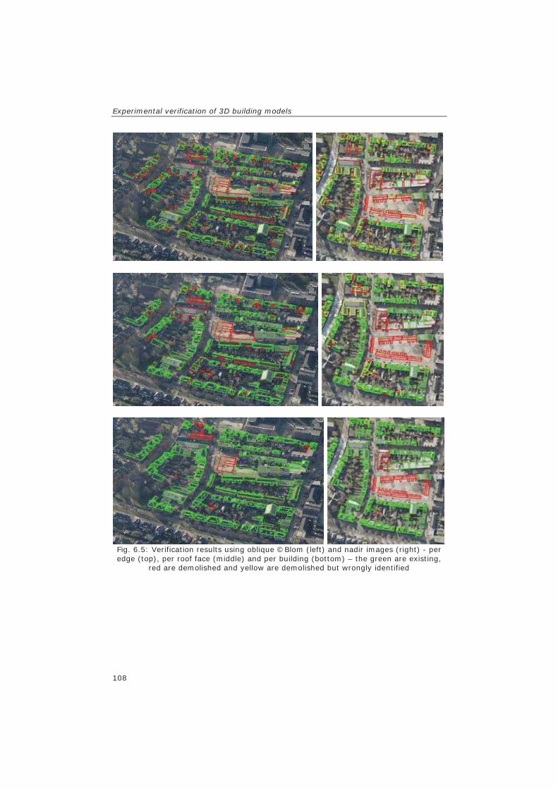
Experimental verification of 3D building models
108
Fig. 6.5: Verification results using oblique ©Blom (left) and nadir images (right) - per edge (top), per roof face (middle) and per building (bottom) – the green are existing,
red are demolished and yellow are demolished but wrongly identified
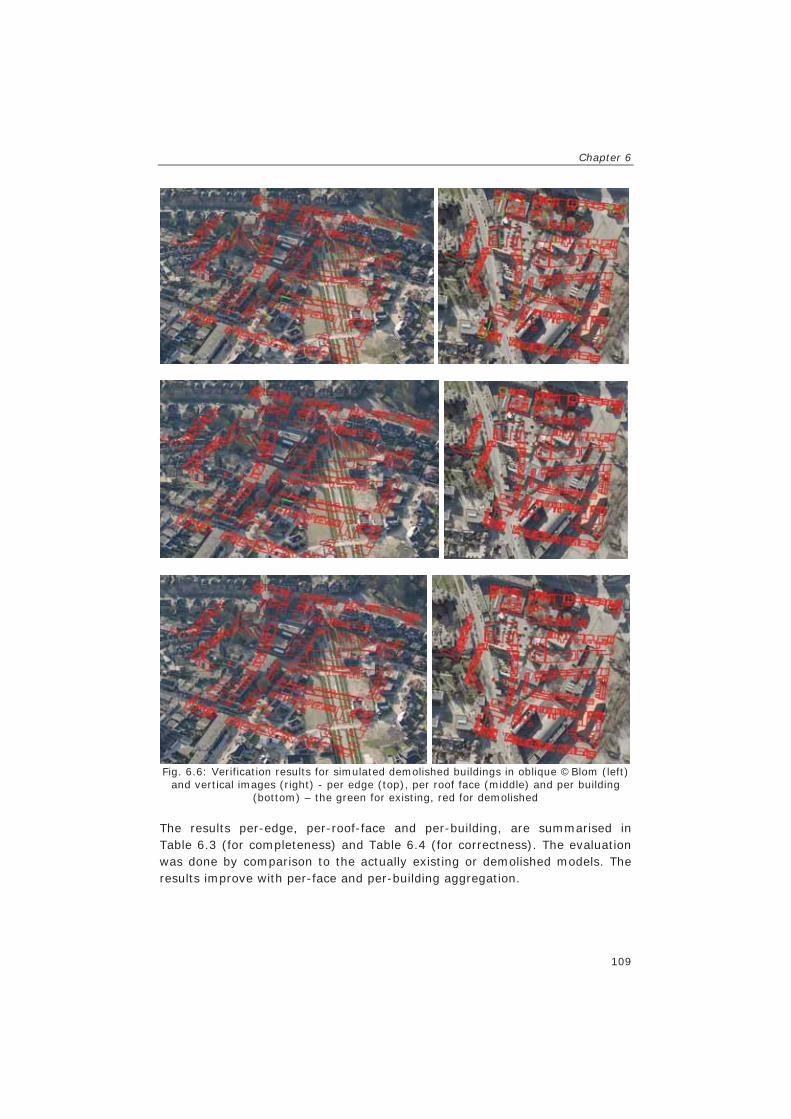
Chapter 6
109
Fig. 6.6: Verification results for simulated demolished buildings in oblique ©Blom (left)
and vertical images (right) - per edge (top), per roof face (middle) and per building (bottom) – the green for existing, red for demolished
The results per-edge, per-roof-face and per-building, are summarised in Table 6.3 (for completeness) and Table 6.4 (for correctness). The evaluation was done by comparison to the actually existing or demolished models. The results improve with per-face and per-building aggregation.

Experimental verification of 3D building models
110
Looking at the per-roof-face results all existing faces were correctly identified in both oblique and vertical images. For the actually demolished (or wrong faces), 2% (9 out of 586) were wrongly categorised as existing for oblique images while for vertical images there were 7% (40 out of 609) faces. For the oblique image the erroneous decision for 9 faces was due to face edges being on some lines in images coincidentally. All these errors occurred in the simulated data. For the nadir images the problem is mainly due to the fact that when a building height is changed (vertical extension), or a model edge is correct in 2D position but wrong in height, the roof face is imaged in nearly the same position (depending on the location of the feature in the image) and the height change is difficult to detect while the height difference is clearly captured in oblique images. This is illustrated in Fig. 6.7 where a wrong face was identified in oblique images but was accepted as correct in vertical images.
Table 6.3: verification results (completeness) obtained by using oblique (Pictometry) and vertical (UltracamD) images
Completeness_ Existing Completness_ Demolished Oblique Vertical Oblique Vertical Per edge 99% 99% 88% 86% Per roof face 100% 100% 98% 93% Per building 100% 100% 100% 97%
Table 6.4: Verification results (correctness) obtained by using oblique (Pictometry) and
vertical (UltracamD) images Correctness _ Existing Correctness_ Demolished
Oblique Vertical Oblique Vertical Per edge 87% 82% 99% 99% Per roof face 98% 91% 100% 100% Per building 100% 97% 100% 100%
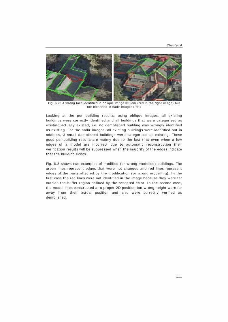
Chapter 6
111
Fig. 6.7: A wrong face identified in oblique image ©Blom (red in the right image) but
not identified in nadir images (left) Looking at the per building results, using oblique images, all existing buildings were correctly identified and all buildings that were categorised as existing actually existed, i.e. no demolished building was wrongly identified as existing. For the nadir images, all existing buildings were identified but in addition, 3 small demolished buildings were categorised as existing. These good per-building results are mainly due to the fact that even when a few edges of a model are incorrect due to automatic reconstruction their verification results will be suppressed when the majority of the edges indicate that the building exists. Fig. 6.8 shows two examples of modified (or wrong modelled) buildings. The green lines represent edges that were not changed and red lines represent edges of the parts affected by the modification (or wrong modelling). In the first case the red lines were not identified in the image because they were far outside the buffer region defined by the accepted error. In the second case, the model lines constructed at a proper 2D position but wrong height were far away from their actual position and also were correctly verified as demolished.

Experimental verification of 3D building models
112
Fig. 6.8: Building models with some correct and wrong edges - red lines are correctly
identified as wrong - images©Blom
6.5 Results from images with different overlaps and resolution
The following are results obtained by using our method applied for verification of building models by using Pictometry and Slagboom en Peeters images. Slagboom en Peeters images are of higher overlap and resolution. More details on these images are in Section 4.2.2. In the verified data, most buildings represented actually existed and were correctly modelled. A few buildings were demolished (or wrongly modelled) and additional wrong models were obtained by simulation. The numbers for roof faces and buildings are shown in Table 6.5. The results for individual edges were combined per roof face and per building as discussed in Section 5.3.4.
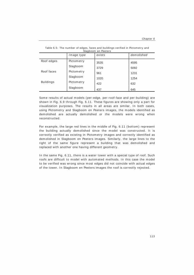
Chapter 6
113
Table 6.5: The number of edges, faces and buildings verified in Pictometry and Slagboom en Peeters
Image type exists demolished
Roof edges Pictometry 3535 4595 Slagboom 3729 5092
Roof faces Pictometry 961 1231 Slagboom 1020 1254
Buildings Pictometry 422 632 Slagboom 437 645
Some results of actual models (per-edge, per-roof-face and per-building) are shown in Fig. 6.9 through Fig. 6.11. These figures are showing only a part for visualization purposes. The results in all areas are similar. In both cases, using Pictometry and Slagboom en Peeters images, the models identified as demolished are actually demolished or the models were wrong when reconstructed. For example, the large red lines in the middle of Fig. 6.11 (bottom) represent the building actually demolished since the model was constructed. It is correctly verified as existing in Pictometry images and correctly identified as demolished in Slagboom en Peeters images. Similarly, the large lines to the right of the same figure represent a building that was demolished and replaced with another one having different geometry. In the same Fig. 6.11, there is a water tower with a special type of roof. Such roofs are difficult to model with automated methods. In this case the model to be verified was wrong since most edges did not coincide with actual edges of the tower. In Slagboom en Peeters images the roof is correctly rejected.

Experimental verification of 3D building models
114
Fig. 6.9: Verification results (per edge) using oblique ©Blom (top) and Slagboom en
Peeters images (bottom) – green for correct and red for demolished (or wrong)
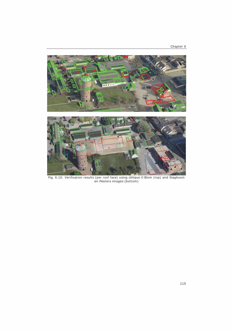
Chapter 6
115
Fig. 6.10: Verification results (per roof face) using oblique ©Blom (top) and Slagboom
en Peeters images (bottom)
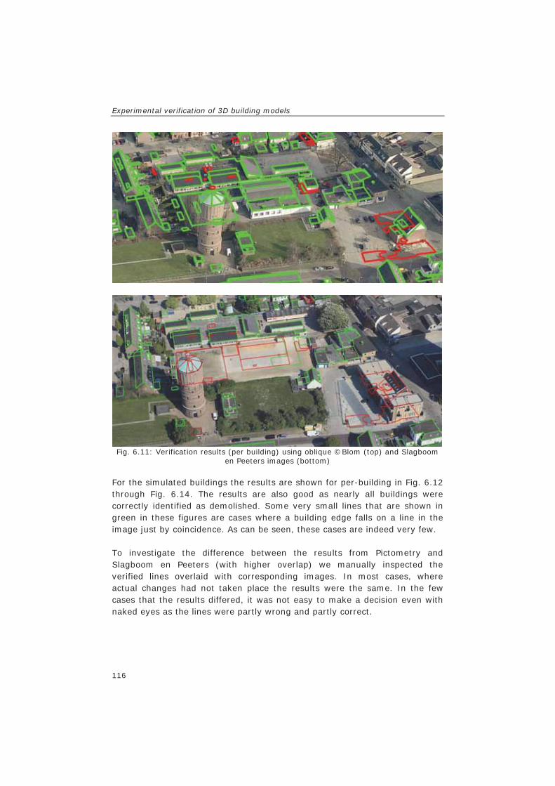
Experimental verification of 3D building models
116
Fig. 6.11: Verification results (per building) using oblique ©Blom (top) and Slagboom
en Peeters images (bottom) For the simulated buildings the results are shown for per-building in Fig. 6.12 through Fig. 6.14. The results are also good as nearly all buildings were correctly identified as demolished. Some very small lines that are shown in green in these figures are cases where a building edge falls on a line in the image just by coincidence. As can be seen, these cases are indeed very few. To investigate the difference between the results from Pictometry and Slagboom en Peeters (with higher overlap) we manually inspected the verified lines overlaid with corresponding images. In most cases, where actual changes had not taken place the results were the same. In the few cases that the results differed, it was not easy to make a decision even with naked eyes as the lines were partly wrong and partly correct.

Chapter 6
117
Fig. 6.12: Verification results (per edge) for simulated buildings using oblique ©Blom
(top) and Slagboom en Peeters images (bottom)
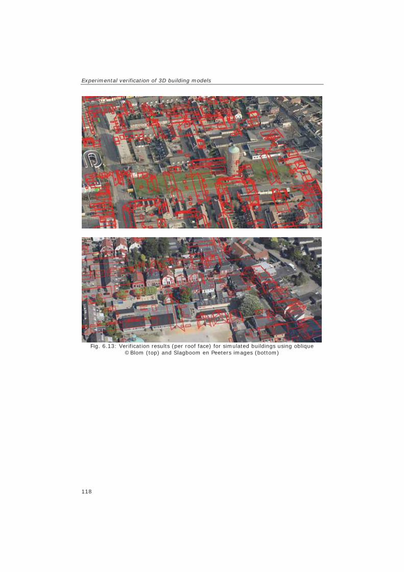
Experimental verification of 3D building models
118
Fig. 6.13: Verification results (per roof face) for simulated buildings using oblique
©Blom (top) and Slagboom en Peeters images (bottom)

Chapter 6
119
Fig. 6.14: Verification results (per building) for simulated buildings using oblique
©Blom (top) and Slagboom en Peeters images (bottom) The results at per-roof-face and per-building for these buildings are summarised in Table 6.6 (for completeness) and Table 6.7 (for correctness). The analysis was done at per roof face and building level. The edges were very many and the visual inspection and classification of each of them could not be done.
Table 6.6: verification results (completeness) obtained by using Pictometry and Slagboom en Peeters images
Completeness_Existing Completness_Demolished
Pictometry Slagboom Pictometry Slagboom Per roof face 100% 100% 99% 98% Per building 100% 100% 99% 98%
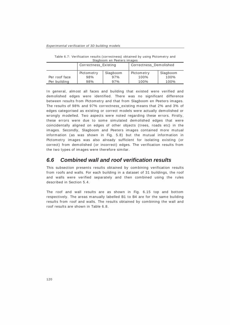
Experimental verification of 3D building models
120
Table 6.7: Verification results (correctness) obtained by using Pictometry and Slagboom en Peeters images
Correctness_Existing Correctness_Demolished
Pictometry Slagboom Pictometry Slagboom Per roof face 98% 97% 100% 100% Per building 98% 97% 100% 100%
In general, almost all faces and building that existed were verified and demolished edges were identified. There was no significant difference between results from Pictometry and that from Slagboom en Peeters images. The results of 98% and 97% correctness_existing means that 2% and 3% of edges categorised as existing or correct models were actually demolished or wrongly modelled. Two aspects were noted regarding these errors. Firstly, these errors were due to some simulated demolished edges that were coincidentally aligned on edges of other objects (trees, roads etc) in the images. Secondly, Slagboom and Peeters images contained more mutual information (as was shown in Fig. 5.8) but the mutual information in Pictometry images was also already sufficient for isolating existing (or correct) from demolished (or incorrect) edges. The verification results from the two types of images were therefore similar.
6.6 Combined wall and roof verification results This subsection presents results obtained by combining verification results from roofs and walls. For each building in a dataset of 31 buildings, the roof and walls were verified separately and then combined using the rules described in Section 5.4. The roof and wall results are as shown in Fig. 6.15 top and bottom respectively. The areas manually labelled B1 to B4 are for the same building results from roof and walls. The results obtained by combining the wall and roof results are shown in Table 6.8.

Chapter 6
121
Fig. 6.15: Roof (top) and wall (bottom) verification results – green for correct, red for
wrong and yellow for undecided
Table 6.8: Combined wall and roof verification results Building# Model status Roof
results Wall
results Combined results
B1 building not changed correct incorrect building not
changed
B2 building not changed correct undecided building not
changed
B3 building modified (wrong model) incorrect undecided building
demolished
B4 building modified (wrong model) incorrect correct building modified
vertically Other 27 buildings
building not changed correct correct building not
changed In the Table 6.8, the first column represents buildings as labelled in Fig. 6.15. The second column shows the status of buildings in reality. Most buildings are not changed but some were wrongly modelled (B3 and B4). The third and fourth columns show results obtained by verifying roofs and walls respectively and the last column shows the combined results. For all the 27 unchanged buildings with both roof and wall results correctly specifying the buildings as not changed, combined results also correctly indicated that the buildings were not changed.
Experimental verification of 3D building models
122
The building labelled B1 was wrongly classified as demolished in the wall results but, by using the criteria that categorises such results as erroneous if the building is categorised as not changed in the roof results, the combined results correctly indicated that the building was not changed. The building labelled B2 was classified (in the wall results) as undecided because most walls were occluded by other objects. The combined result was based on only roof verification and correctly indicated that the building was not changed. The roof of the building labelled B3 was actually wrongly modelled. The walls results were undecided and the roof was identified as incorrect, i.e. a right decision. The combined result was based only on the roof and the building was categorised as demolished. This result was not completely correct. Building labelled B4 is also for the actually wrongly modelled roof. The building was classified as demolished in the roof results but, by using the criteria that categorises such results as modified vertically if the building is categorised as correct in the wall results, the combined results correctly indicated that the building was modified. All the cases discussed above point to the conclusion that the combination of wall and roof information results to better verification of building models.
6.7 Discussion The results presented in this chapter indicate that oblique images are useful for verification of 3D building models. The method developed is useful for identifying buildings that exist or are demolished or modified since models were acquired. It is also useful for verifying wrongly modelled buildings. The roof verification experiments were done by using mutual information obtained in an unsupervised manner with random edges automatically extracted from the images. In our experiments, although the roof verification results from oblique images were similar to nadir images for most cases, oblique images were particularly better in the cases where the differences or changes were in vertical direction. Thus, oblique images are good for identifying developments such as vertical extensions of buildings. Although the size of overlap (i.e number of images in which edges of a building model are visible) is important, in the roof verification experiments the added advantage was not considerable as roof faces were already visible

Chapter 6
123
in many images even with the comparatively lowly overlapping Pictometry images. The combination of wall and roof verification results has shown that the information is complementary. The method is particularly useful for identifying vertically modified buildings, either through extension or partly demolishment, like a pancake collapse caused by an earthquake. The method is also useful for detecting wrong 3D roof models. These cases are recognised when roofs are verified as incorrect and walls are verified as correct.

Experimental verification of 3D building models
124
125
7. Conclusion and Recommendations In this thesis we have presented methods for automatic verification of two-dimensional building datasets and three-dimensional building models. In both methods, we used oblique airborne images which contain top and side views of buildings. The main contribution of this work is the modelling of information in oblique images for identifying existing, demolished and modified buildings. This chapter presents the conclusion from the study (Section 7.1) and recommendations for future research (Section 7.2).
7.1 Conclusion This research was conducted during a period that has witnessed fast increase in the systematic acquisition of airborne oblique images. A number of companies have captured large datasets. These include Pictometry (and their licensees Blom) and Slagboom en Peeters Luchtfotografie B.V. Even more interesting are continuous announcements of development of new cameras systems including the Microsoft’s Osprey (Osprey, 2013), the Leica RCD30 5-head for the mid-format (Leica-Geosystems, 2013), the IGI Penta DigCam (IGI, 2013b) and the rotating MapVision’s A3 camera (A3, 2013). In this work we have shown that utilization of airborne oblique images for automatic verification of buildings is feasible. For 2D building verification, the 2D outlines are converted to 3D wall hypotheses and then features based on edges and texture of walls in multi-perspective images are automatically computed and compared. In this case, a number of issues were noted as important. Firstly, the results have shown that the clues identified and modelled to obtain verification measures were useful for building verification. A second issue that proved to be very important was the approach for combining the different measures for possible existence of a wall in images. In our tests with AdaBoost, RTrees and Hints, we realized that in most cases AdaBoost produced the best results. The third aspect relates to the need for identification of occluded (sides of) buildings which would otherwise be confused with demolished ones. For this purpose, our procedure for visibility analysis proved to be very useful. The procedure uses a point cloud generated from the same oblique images, thanks to already existing image matching methods. Regarding the evaluation, the completeness and correctness obtained (around 90 - 100%) was very encouraging. Our method verifies individual walls and then combines the results to obtain the per-building status. The
Conclusions and recommendations
126
procedure proved useful for identifying not only completely existing and completely demolished buildings but also modified buildings. For the 3D case, Mutual Information was modelled for verification of roofs. Some important issues are also noted. The first is that the oblique images proved more useful than the nadir images, particularly for identifying buildings extended in vertical direction or poorly modelled. The second aspect relates to spatial resolution and overlap of image. Tests with images of higher overlap and resolution (Slagboom en Peeters) gave more mutual information but the mutual information in the relatively lower resolution (Pictometry) images was already sufficient and the verification results from the two types of images were similar. The other issue is related to parts of buildings that are appropriate for verification of the buildings by using images. In this case, combining roof and wall information proved to be more useful than when using only roof or wall information alone. Although some researchers argue that a complete and general building extraction system probably will never be possible (Baltsavias, 2004; Kaartinen et al., 2005; Mayer, 2008), we have shown that good results can be achieved for the subtask of automatic verification of existing datasets.
7.2 Recommendations For purpose of verification of 2D-building outlines, a number of measures were developed for identification of wall faces in airborne oblique images. In order to improve the verification, more studies may be done to formulate new measures. As the procedure for combining these measures (i.e by using AdaBoost, RTrees or Hints) is not limited to a specific number of measures, the new measures may be added to the ones developed in this work straight away. One of the measures used in the verification of the 2D building outlines is the Line Match Ratio. This measure requires some façade edges to be available in more than one image taken from different perspectives. The method also requires the edges to be extracted in both images and compared in object space. However, sometimes different lines are extracted in the different perspective images and the comparison results to a wrong verification of a wall. This happened due to the difference in perspective, illumination and also the thresholds in the line extraction algorithms. In the future, tests may be conducted by extracting lines in one of the perspective images and seek evidence of existence of lines in the corresponding positions in the other
Chapter 7
127
images. The Mutual Information approach may was used in this work but only for verification of 3D model edges may be one alternative to be tried for this purpose. In this work, verification of 2D building outlines only used wall hypothesis and only oblique images. For future work, if ortho-rectified images of the same areas are also available, verification of a building may use additional information from the roof. Although this may not give information at per-wall level, it presumably will improve results for existing and demolished buildings. In our work, the verification of 2D building outlines is preceded by selecting some buildings with existing and demolished walls to be used as training data. In the future, efforts may be on how to make the verification of walls unsupervised. The results obtained in 3D building model verification can also be used for checking the quality of 3D building modelling. If the building exists and most faces are correct the verification results for a 3D model automatically reconstructed will indicate that the building exists. Individual faces with results contrary to the overall may be updated. This may be done manually but automatic updating of 3D models using image information is an interesting future work. Our 2D method requires some height information for constructing a wall hypothesis and visibility analysis. The height information was obtained from a point cloud derived from the same oblique images by using image matching methods. A point cloud generated this way is noisy and may contain some gaps. Research for improved point clouds from images will therefore benefit the verification.

Conclusions and recommendations
128
129
Bibliography A3, 2013. A3 Technology, http://www.visionmap.com/en/technology,
(Accessed 27 March, 2013). Agouris, P., Stefanidis, A., Gyftakis, S., 2001. Differential snakes for change
detection in road segments. Photogrammetric Engineering and Remote Sensing 67 (12), 1391-1400.
Alobeid, A., Jacobsen, K., Heipke, C., Al Rajhi, M., 2011. Building Monitoring with Differential DSMs. International Archives of Photogrammetry, Remote Sensing and Spatial Information Sciences 38(4/W19), (on CDROM).
Arandiga, F., Cohen, A., Donat, R., Matei, B., 2010. Edge detection insensitive to changes of illumination in the image. Image and Vision Computing 28 (4), 553-562.
Armenakis, C., Jung, J., Sohn, G., 2010. Practices and Trends in Geospatial Change Determination. International Archives of Photogrammetry, Remote Sensing and Spatial Information Sciences 38 (4), (on CDROM).
Baltsavias, E.P., 2004. Object extraction and revision by image analysis using existing geodata and knowledge: current status and steps towards operational systems. ISPRS Journal of Photogrammetry and Remote Sensing 58 (3-4), 129-151
Boudet, L., Paparoditis, N., Jung, F., Martinoty, G., Pierrot-Deseilligny, M., 2006. A supervised classification approach towards quality self-diagnosis of 3D building models using digital aerial imagery. International Archives of Photogrammetry, Remote Sensing and Spatial Information Sciences 36 (3), 136-141.
Bouziani, M., Goïta, K., He, D.-C., 2010. Automatic change detection of buildings in urban environment from very high spatial resolution images using existing geodatabase and prior knowledge. ISPRS Journal of Photogrammetry and Remote Sensing 65 (1), 143-153.
Bouziani, M., Goita, K., Dong-Chen, H., 2007. Change detection of buildings in urban environment from high spatial resolution satellite images using existing cartographic data and prior knowledge, Geoscience and Remote Sensing Symposium. IGARSS 2007. IEEE International, pp. pp. 2581-2584.
Breiman, L., 2001. Random forests. Machine Learning 45 (1), 5-32. Burns, J.B., Hanson, A.R., Riseman, E.M., 1986. Extracting straight lines.
IEEE Transactions on Pattern Analysis and Machine Intelligence 8 (4), 425-455.
Canny, J., 1986. A computational approach to edge detection. IEEE Trans. Patt. Anal. Mach. PAMI-8, 6, , 679-698.
Carlsson, C., Fullér, R., 1996. Fuzzy multiple criteria decision making: Recent developments. Fuzzy Sets and Systems 78 (2), 139-153.

Bibliography
130
Champion, N., Boldo, D., Pierrot-Deseilligny, M., Stamon, G., 2010. 2D building change detection from high resolution satelliteimagery: A two-step hierarchical method based on 3D invariant primitives. Pattern Recognition Letters 31 (10), 1138-1147.
Champion, N., Matikainen, L., Liang, X., Hyyppä, J., Rottensteiner, F., 2008. A Test of 2D Building Change Detection Methods: Comparison, Evaluation and Perspectives. International Archives of Photogrammetry, Remote Sensing and Spatial Information Sciences 37 (Part B4), 297-305.
Champion, N., 2007. 2D building change detection from high resolution aerial images and correlation Digital Surface Models. International Archives of Photogrammetry, Remote Sensing and Spatial Information Sciences 36 (3/W49A), 197–202.
Christoudias, C.M., Georgescu, B. and Meer, P. , 2002. Synergism in low level vision. Proc. 16th International Conference on Pattern Recognition. Track 1: Computer Vision and Robotics, Quebec City, Canada, pp. 150-155.
Dempster, A., 1967. Upper and Lower Probabilities Induced by a Multivalued Mapping. Annals of Mathematical Statistics 38 (2), 325-339.
Ehlers, M., Klonus, S., DTomowski, a., Michel, U., Reinartz, P., 2010. Automated Change Detection From High-Resolution Remote Sensing Images. International Archives of Photogrammetry, Remote Sensing and Spatial Information Sciences 38 (4), (on CDROM).
Förstner, W., 1996. 10 Pros and Cons Against Performance Characterization of Vision Algorithms. Proc. Performance Characteristics of Vision Algorithms, Cambridge.
Förstner, W., 1994. A framework for low level feature extraction, Computer Vision - ECCV '94, pp. 383-394.
Freund, Y., Schapire, R.E., 1997. A Decision-Theoretic Generalization of On-Line Learning and an Application to Boosting. Journal of Computer and System Sciences 55 (1), 119-139.
Frueh, C., Sammon, R., Zakhor, A., 2004. Automated texture mapping of 3D city models with oblique aerial imagery, 3DPVT. IEEE Computer Society, pp. 396-403.
Fugro-Aerial-Mapping-B.V., 2011. Imagery, http://www.flimap.com/site6.php, (Accessed 6 March, 2011).
Furukawa, Y., Ponce, J., 2010. Accurate, Dense, and Robust Multi-View Stereopsis. IEEE Transactions on Pattern Analysis and Machine Intelligence 32 (8), 1362-1376.
Gerke, M., 2011. Using horizontal and vertical building structure to constrain indirect sensor orientation. ISPRS Journal of Photogrammetry and Remote Sensing 66 (3), 307-316.

Bibliography
131
Gerke, M., Kerle, N., 2011. Automatic structural seismic damage assessment with airborne oblique pictometry imagery. PE&RS = Photogrammetric Engineering and Remote Sensing 77 (9), 885-898.
Gerke, M., 2009. Dense matching in high resolution oblique airborne images. International Archives of Photogrammetry, Remote Sensing and Spatial Information Sciences 38 (Part 3/W4), 77-82.
Gerke, M., Heipke, C., 2008. Image†based quality assessment of road databases X. International Journal of Geographical Information Science 22 (8), 871-894.
Gioi, R.G.v., Jakubowicz, J., Morel, J.-M., Randall, G., 2008. LSD: A Fast Line Segment Detector with a False Detection Control. IEEE Transactions on Pattern Analysis and Machine Intelligence 99
Grenzdörffer, G.J., Guretzki, M., Friedlander, I., 2008. Photogrammetric image acquisition and image analysis of oblique imagery. The Photogrammetric Record 23 (124), 372-386.
Gruber, M., 2007. UltraCamX, the new digital aerial camera system by Microsoft Photogrammetry, Proceedings of the Photogrammetric Week Stuttgart pp. 137-145.
Gruen, A., Zhang, L., 2003. Sensor Modeling for Aerial Triangulation with Three-Line-Scanner (TLS) Imagery. Journal of Photogrammetrie, Fernerkundung, Geoinformation 2/2003, 85-98.
Haala, N., 2011. Multiray Photogrammetry and Dense Image Matching, Photogrammetric Week 2011. Wichmann Verlag, Berlin/Offenbach, pp. 185-195.
Haala, N., Kada, M., 2010. An update on automatic 3D building reconstruction. ISPRS Journal of Photogrammetry and Remote Sensing 65 (6), 570-580.
Heipke, C., Pakzad, K., Willrich, F., Peled, A., 2004. Theme Issue: Integration of Geodata and Imagery for Automated Refinement and Update of Spatial Databases. ISPRS Journal of Photogrammetry and Remote Sensing 58 (3-4), 127-128.
Hirschmüller, H., 2008. Stereo processing by Semi-Global Matching and Mutual Information IEEE Transactions on Pattern Analysis and Machine Intelligence 30(2), 328-341.
Höhle, J., 2008. Photogrammetric Measurements in Oblique Aerial Images. Photogrammetrie Fernekundung Geoinformation 2008 (1), 7-14.
Holland, D., Boyd, D., Marshall, P., 2006. Updating topographic mapping in Great Britain using imagery from high-resolution satellite sensors. ISPRS Journal of Photogrammetry and Remote Sensing 60 (3), 212-223.
Holland, D., Marshall, P., 2004. Updating Maps in a Well-Mapped Country Using High Resolution Satellite Imagery International Archives of Photogrammetry, Remote Sensing and Spatial Information Sciences 35 (Part B2), 747 -751.

Bibliography
132
Hough, P.V.C., 1962. Methods and Means for Recognizing Complex Patterns U.S. Patent 3069654.
Huertas, A., Nevatia, R., 2000. Detecting changes in aerial views of man-made structures. Image and Vision Computing 18 (8), 583-596.
IGI, 2013a. Nadir & Oblique Imagery, perfectly suited for 3D Texturing, http://www.igi.eu/quattro-digicam.html, (Accessed 10 July, 2013).
IGI, 2013b. Penta DigiCAM Specifications, http://www.igi.eu/penta-digicam.html, (Accessed 10 July, 2013).
Ioannidis, C., Psaltis, C., Potsiou, C., 2009. Towards a strategy for control of suburban informal buildings through automatic change detection. Computers, Environment and Urban Systems 33 (1), 64-74.
Kaartinen, H., Hyyppä, J., Gülch, E., Vosselman, G., Hyyppä, H., Matikainen, L., Hofmann, A.D., Mäder, U., Söderman, J., Elmqvist, M., Ruiz, A., Dragoja, M., Flamanc, D., Maillet, G., Kersten, T., Carl, J., Hau, R., Wild, E., Frederiksen, L., Holmgaard, J., Vester, K., 2005. Accuracy of 3d City Models: EuroSDR comparison. International Archives of Photogrammetry, Remote Sensing and Spatial Information Sciences 36 (Part 3/W19), 227-232.
Knudsen, T., 2007. An algorithm for verification and change detection between 3D geospatial databases and aerial images. International Archives of Photogrammetry, Remote Sensing and Spatial Information Sciences 36 (Part 1/W51), (on CDROM).
Kohlas, J., Monney, P., 1995. A mathematical theory of hints - an approach to the Dempster-Shafer theory of evidence. Springer, Berlin.
Kolbe, T.H., Gröger, G., Plümer, L., 2005. CityGML - Interoperable Access to 3D City Models. In: Oosterrom, Zlatanova and Fendel (Editors), Int. Symposium on Geo-information for Disaster Management. Springer Verlag, Delft.
Kumar, P., Mittal, A., Kumar, P., 2009. Addressing uncertainty in multi-modal fusion for improved object detection in dynamic environment. Information Fusion 11 (4), 311-324.
Kuncheva, L., 2004. Combining pattern classifiers: methods and algorithms. Wiley-Interscience.
Kurz, F., Charmette, B., Suri, S., Rosenbaum, D., Spangler, M., Leonhardt, A., Bachleitner, M., Stätter, R., Reinartz, P., 2007a. Automatic traffic monitoring with an airborne wide-angle digital camera system for estimation of travel times. International Archives of Photogrammetry, Remote Sensing and Spatial Information Sciences 36 (Part 3/W49A), pp. 83-88.
Kurz, F., Müller, R., Stephani, M., Reinartz, P., Schroeder, M., 2007b. Calibration of a wide-angle digital camera system for near real time scenarios. International Archives of Photogrammetry, Remote Sensing and Spatial Information Sciences 36 (Part 1/W51), (on CD-ROM).

Bibliography
133
Le Besnerais, G., Sanfourche, M., Champagnat, F., 2008. Dense height map estimation from oblique aerial image sequences. Computer vision and image understanding 109 (2), 204-225.
Le Bris, A., Chehata, N., 2011. Change detection in a topographic building database using sub-metric satellite images. International Archives of Photogrammetry, Remote Sensing and Spatial Information Sciences 38 (3/W22), (on CDROM).
Leica-Geosystems, 2013. Leica RCD30 Oblique, http://www.leica-geosystems.com/en/Leica-RCD30-Oblique_99831.htm, (Accessed 10 July, 2013).
Lemmen, M., Lemmen, C.H.J., Wubbe, M., 2007. Pictometry : potentials for land administration. Proc. 6th FIG regional conference, San José, Costa Rica, 12-15 November, 13 p.
Lemmens, M., Lemmen, C.H.J., 2007. Pictometry : long - term impact on GI market : GIM interviews Arne Saugstad and Nils A. Karbo, Blom group. GIM international : the global magazine for geomatics 21 (4).
Lowe, D.G., 2004. Distinctive image features from scale invariant keypoints. International Journal of Computer Vision 60 (2), 91-110.
Lowe, D.G., 1987. Three-dimensional object recognition from single two-dimensional images. Artificial intelligence 31 (3), 355-395.
Matikainen, L., Kaartinen, K., Hyyppä, J., 2007. Classification tree based building detection from laser scanner and aerial image data. International Archives of Photogrammetry, Remote Sensing and Spatial Information Sciences 36 (Part 3/W52), 280-287.
Maudes, J., Rodriguez, J., Garcia-Osorio, C., Garcia-Pedrajas, N., 2012. Random Feature Weights for Decision Tree Ensemble Construction. Information Fusion 13 (1), 20-30.
Mayer, H., 2008. Object extraction in photogrammetric computer vision. ISPRS Journal of Photogrammetry & Remote Sensing 63, 213-222.
McClone, J.C.e., Mikhail, E.M.e., Bethel, J.S.e. (Editors), 2004. Manual of photogrammetry. American Society for Photogrammetry and Remote Sensing (ASPRS), Bethesda, 1151 pp.
Meixner, P., Leberl, F., 2010. Interpreting building façades from vertical aerial images using the third dimension. Proc. A special joint symposium of ISPRS Technical Commission IV & AutoCarto Orlando, United States of America, 15-19 November, pp. 55-59.
MIDAS, 2011. Track'Air Aerial Survey Sytems, http://trackair.com/index.php/products/midas/, (Accessed 21 March, 2012).
Mishra, P., Ofek, E., Kimchi, G., 2008. Validation of Vector Data using Oblique Images. Proc. The 16th ACM SIGSPATIAL International Conference on Advances in Geographic Information Systems (ACM GIS 2008), Irvine, California, USA, 5-7 November, pp. 193-202.

Bibliography
134
Nakagawa, M., Shibasaki, R., 2008. Building Change Detection Using 3-D Texture Model. International Archives of Photogrammetry, Remote Sensing and Spatial Information Sciences 37 (Part B3a), 173-178.
Nyaruhuma, A.P., Gerke, M., Vosselman, G., 2012a. Verification of 3D building models using mutual information in airborne oblique images. ISPRS Annals I-3, 275-280.
Nyaruhuma, A.P., Gerke, M., Vosselman, G., Mtalo, E.G., 2012b. Verification of 2D building outlines using oblique airborne images. ISPRS Journal of Photogrammetry and Remote Sensing 71, 62-75.
Nyaruhuma, A.P., 2010. Automatic identification of buildings demolished by disasters using oblique images. Proc. AARSE 2010 : 8th international conference African Association of Remote Sensing of the Environment, AARSE, on earth observation for Africa's development agenda, Addis Ababa, Ethiopia, 163 p.
Nyaruhuma, A.P., Gerke, M., Vosselman, G., 2010a. Evidence of walls in oblique images for automatic verification of buildings. International Archives of Photogrammetry, Remote Sensing and Spatial Information Sciences 38(Part 3A), 263-268.
Nyaruhuma, A.P., Gerke, M., Vosselman, G., 2010b. Line matching in oblique airborne images to support automatic verification of building outlines. Proc. ASPRS Annual Conference, San Diego, 26-30 April, (on CDROM).
Olsen, B.P., 2004. Automatic change detection for validation of digital map databases. International Archives of Photogrammetry, Remote Sensing and Spatial Information Sciences 35 (Part B2), 569 - 574.
Olsen, B.P., Knudsen, T., Frederiksen, P., 2002. Hybrid Raster/Vector Change Detection for Map Database Update. Proc. DSAGM, Copenhagen, Denmark, pp. 41-46
Osprey, 2013. Microsoft Introduces New Oblique UltraCam Osprey, http://www.gisuser.com/content/view/29447/2/, (Accessed 27 March, 2013).
Oude Elberink, S., Vosselman, G., 2011. Quality analysis on 3D building models reconstructed from airborne laser scanning data. ISPRS Journal of Photogrammetry and Remote Sensing 66 (2), 157-165.
Oude Elberink, S., Vosselman, G., 2009. Building Reconstruction by Target Based Graph Matching on Incomplete Laser Data: Analysis and Limitations. Sensors 9 (8), 6101-6118.
Petrie, G., 2009. Systematic oblique aerial photography using multi frame cameras. Photogrammetric Engineering & Remote Sensing 75 (2), 102-108.
Petrie, G., Walker, A.S., 2007. Airborne digital imaging technology: a new overview. The Photogrammetric Record 22 (119), 203-225.
Rottensteiner, F., 2007. Building change detection from Digital Surface Models and multi-spectral images. International Archives of

Bibliography
135
Photogrammetry, Remote Sensing and Spatial Information Sciences 36 (Part 3/W49B), (on CD-ROM).
Sasikala, K.R., Petrou, M., 2001. Generalised fuzzy aggregation in estimating the risk of desertification of burned forest. Fuzzy Sets and Systems 118 (1), 121-137.
Shafer, G., 1976. A Mathematical Theory of Evidence. Princeton University Press, Princeton.
Shannon, C.E., 1948. A mathematical theory of communication. Bell Systems Technical Journal 27, 379-423 and 623-656.
Slama, C.C.e., Theurer, C.e., Henriksen, S.W.e. (Editors), 1980. Manual of photogrammetry. American Society of Photogrammetry ASP, Falls Church, 1056 pp.
Suveg, I., Vosselman, M.G., 2004. Reconstruction of 3D building models from aerial images and maps. ISPRS Journal of Photogrammetry and Remote Sensing 58 (3-4), 202-224.
Suveg, I., Vosselman, G., 2002. Mutual information based evaluation of 3D building models, Pattern Recognition, 2002. Proceedings. 16th International Conference on, pp. 557-560.
Taneja, A., Ballan, L., Pollefeys, M., 2011. Image Based Detection of Geometric Changes in Urban Environments. Proc. 13th International Conference on Computer Vision (ICCV2011), Barcelona, Spain, (on CDROM).
Vögtle, T., Steinle, E., 2004. Detection and recognition of changes in building geometry derived from multitemporal laserscanning data. International Archives of Photogrammetry and Remote Sensing 35(B2), 428-433.
Vosselman, G., Gorte, B.G.H., Sithole, G., 2004. Change detection for updating medium scale maps using laser altimetry. International Archives of Photogrammetry, Remote Sensing and Spatial Information Sciences 35 (Part B3), 207-212.
Vosselman, G., 1992. Relational matching. Lecture Notes in Computer Science, 628. Springer, Berlin, 190 pp.
Walter, V., 2004. Object-based classification of remote sensing data for change detection. ISPRS Journal of Photogrammetry & Remote Sensing Sensing 58, 225-238.
Walter, V., Fritsch, D., 2000. Automated revision of GIS databases. Proc. The Eight ACM Symposium on Advances in Geographic Information Systems, pp. 129-134.
Wang, M., Bai, H., Hu, F., 2008a. Automatic Texture Acquisition for 3D Model Using Oblique Aerial Images. Proc. First International Conference on Intelligent Networks and Intelligent Systems, Beijing, China, pp. 495-498.
Wang, Y., Schultz, S., Giuffrida, F., 2008b. Pictometry's Proprietary Airborne Digital Imaging System and its Application in 3D City Modelling.

Bibliography
136
International Archives of Photogrammetry, Remote Sensing and Spatial Information Sciences 37 (Part B1), 1065-1070.
Xiao, J., Gerke, M., Vosselman, G., 2012. Building extraction from oblique airborne imagery based on rubust facade detection. ISPRS journal of photogrammetry and remote sensing 68, 56-68.
Zadeh, L.A., 1965. Fuzzy sets. Information and Control 8 (3), 338-353. Zebedin, L., Klaus, A., Gruber, B., Karner, K., 2006b. Facade Reconstruction
from Aerial Images by Multi-View Plane Sweeping. International Archives of Photogrammetry, Remote Sensing and Spatial Information Sciences 36 (Part 3), 31-36.
Zhang, C., 2004. Towards an operational system for automated updating of road databases by integration of imagery and geodata. ISPRS Journal of Photogrammetry and Remote Sensing 58 (3-4), 166-186.

137
Summary The world has recently witnessed fast increase in systematic acquisition of airborne oblique images with scenes taken from multiple directions. Companies with large datasets include Pictometry (and their licensees Blom) and Slagboom en Peeters Luchtfotografie B.V. More interesting are continuous announcements of development of new camera systems including the Microsoft’s Osprey, the Leica RCD30 5-head, the IGI Penta DigCam and the rotating MapVision’s A3 camera. This research investigated the usefulness of oblique airborne images for automatic verification of buildings in topographic datasets. Existing building verification methods utilize colour, texture and height from vertical images or range data. Oblique images, which contain top as well as side views of imaged objects, are not commonly used. In this work, two methods were developed, the first for verification of building outlines in two-dimensional (2D) large scale topographic databases and the second for verification of 3D building models. In both methods, the vector data was fitted to multiple oblique images and features derived from the images were used to do the verification. For 2D building verification, the 2D outlines were converted to 3D wall hypotheses and then features based on edges and texture of walls in multi-perspective images were automatically computed and compared. In this case, a number of issues were noted as important. Firstly, the results have shown that the clues identified and modelled to obtain verification measures were useful for building verification. A second issue noted as important is the approach for combining the different measures for possible existence of a wall in images. In the developed method, verification of 2D building outlines starts by checking individual walls of a building and then the results are combined for overall verification of the building. A number of features suitable for recognising a wall in oblique images were therefore developed and strategies to combine these features in an overall measure of the status of a wall and a building were designed and tested. In our tests for combining wall verification measures with Adaptive Boosting, Random Trees and a variant of the Dempster-Shafer (Hints), the results showed minor differences but in most cases Adaptive Boost produced the best results. The third aspect relates to the need for identification of occluded (sides of) buildings which would otherwise be confused with demolished ones. For this purpose, our procedure for visibility analysis proved to be very useful. The

Summary
138
procedure uses a point cloud generated from the same oblique images, thanks to already existing image matching methods. Regarding the evaluation, the completeness and correctness obtained (around 90 - 100%) was very encouraging. As the method verifies individual walls and then combines the results to obtain the per-building status, the method identifies not only completely existing or demolished buildings but also buildings that may have changed by part demolition or extension. These are signalled when only some walls of a building are identified in the images. For the 3D case, the problem being tackled is identifying buildings that are demolished or changed since the models were constructed or identifying wrongly constructed models using the images. Automatic method for verification was developed by adopting the theory of Mutual Information. It assumes that the pixel gradient directions computed along a model edge should be generally different from gradient directions computed on random image positions. These gradient directions were found to be very robust for the verification. Some important issues were also noted. Firstly, by concentrating on roofs only we also used the method to test and compare results from nadir images. This comparison made clear that especially height errors in models can be more reliably detected in oblique images than in nadir images because of the tilted view. The second aspect relates to spatial resolution and overlap of image. Tests with images of higher overlap and resolution (Slagboom en Peeters) gave more mutual information but the mutual information in the relatively lower resolution (Pictometry) images was already sufficient and the verification results from the two types of images were similar. The correctness and completeness were between 97% and 100% in both cases. The third issue is related to the parts of a building that are used for verification. The combining roof and wall information proved to be more useful than when using only roof or wall information alone. Although complete and general automation of building extraction is still challenging we have shown that good results can be achieved for the subtask of automatic verification of existing datasets.
139
Samenvatting In de afgelopen jaren is de systematische opname van oblieke luchtfoto’s met opnames vanuit verschillende richtingen snel toegenomen. Onder meer Pictometry (en onder licentie Blom) en Slagboom en Peeters Luchtfotografie B.V. maken dergelijke grote datasets. Nog interessanter zijn verdere aankondigingen van de ontwikkeling van nieuwe camerasystemen zoals Microsoft’s Osprey, de Leica RCD30 5-head, de IGI Penta DigCam en de roterende MapVision’s A3 camera. Dit proefschrift beschrijft onderzoek naar het gebruik van oblieke luchtfoto’s voor de automatische verificatie van gebouwen in topografische datasets. Bestaande methoden voor de verificatie van gebouwen maken gebruik van kleur, textuur en van hoogte afgeleid uit nadir foto’s of uit laser scanning data. Oblieke luchtfoto’s, die zowel een bovenaanzicht als zijaanzicht van objecten bevatten, worden normaal niet gebruikt. In dit onderzoek zijn twee methoden ontwikkeld; de eerste voor de verificatie van gebouwomlijningen in tweedimensionale (2D) grootschalige topografische databases en de tweede voor de verificatie van 3D gebouwmodellen. In beide methoden is vectordata ingepast op meerdere oblieke luchtfoto’s en wordt geverifieerd met behulp van kenmerken die uit de foto’s zijn afgeleid. Voor de 2D verificatie van gebouwen zijn de 2D omlijningen geconverteerd naar 3D muurhypothesen. De kenmerken, die zijn gebaseerd op contrastranden en textuur van de muren in meerdere perspectieve foto’s, zijn automatisch berekend en vergeleken. Meerdere belangrijke aspecten werden geïdentificeerd. In de eerste plaats lieten de resultaten zien dat de geïdentificeerde kenmerken goed bruikbaar waren voor de verificatie van de gebouwen. Een tweede aspect betrof de aanpak om meerdere verschillende kenmerken voor een mogelijke aanwezigheid van een muur in de foto’s met elkaar te combineren. In de ontwikkelde methode start de verificatie van de 2D gebouwomlijningen met de verificatie van de individuele muren en worden de resultaten daarna gecombineerd voor de verificatie van een gebouw. Hiervoor zijn een aantal kenmerken ontwikkeld die geschikt zijn voor de herkenning van muren in oblieke foto’s en zijn strategieën ontworpen en getoetst voor de combinatie van deze kenmerken in een maat voor de herkenning van een muur en een gebouw. Onze testen voor de vergelijking van de muurverificatie met Adaptive Boosting, Random Trees en een variant van Dempster-Shafer (Hints) lieten slechts geringe verschillen zien, maar in de meeste gevallen werd met Adaptive Boost het beste resultaat bereikt.

Samenvatting
140
Het derde aspect heeft te maken met de noodzaak om niet zichtbare (delen van) gebouwen te identificeren, die anders verward zouden kunnen worden met afgebroken gebouwen. Voor dit doel bleek onze procedure voor de zichtbaarheidsanalyse erg nuttig. De procedure maakt gebruik van een puntenwolk die uit de oblieke luchtfoto’s is verkregen met al bestaande image matching methoden. Wat betreft de evaluatie zijn de volledigheid en juistheid (rond 90-100%) zeer bemoedigend. Omdat de methode individuele muren verifieert en dan de resultaten combineert om de status per gebouw te bepalen, stelt de methode niet alleen geheel aanwezige of gesloopte gebouwen vast, maar ook gebouwen die gedeeltelijk zijn gesloopt of uitgebreid. Deze worden gesignaleerd wanneer slechts een deel van de muren van een gebouw zijn geïdentificeerd in de beelden. In het 3D geval worden gebouwen geïdentificeerd, die zijn gesloopt of veranderd, of waarvan het 3D model niet goed was geconstrueerd. Een automatische methode voor de verificatie is ontwikkeld onder gebruikmaking van de theorie van de wederzijdse informatie. Aangenomen wordt dat de gradiëntrichting van de pixels langs de modelranden in het algemeen anders moeten zijn dan de gradiëntrichtingen van willekeurig gekozen pixels. Deze gradiëntrichtingen bleken erg robuust te zijn voor de verificatie. Wederom worden meerdere belangrijke aspecten geïdentificeerd. In de eerste plaats werd door alleen te kijken naar de daken de methode ook toegepast en vergeleken met resultaten die met nadirluchtfoto’s werden verkregen. Deze vergelijking maakte duidelijk dat in het bijzonder fouten in de hoogte van de modellen betrouwbaarder in oblieke luchtfoto’s kunnen worden vastgesteld vanwege het schuine aanzicht. Het tweede aspect betreft de ruimtelijke resolutie en de overlap tussen de beelden. Tests met beelden met een grotere overlap en hogere resolutie (Slagboom en Peeters) resulteerden in meer wederzijdse informatie, maar de wederzijdse informatie in de beelden met relatief lage resolutie (Pictometry) was al voldoende en de verificatieresultaten van beide typen foto’s waren vergelijkbaar. De juistheid en volledigheid waren in beide gevallen tussen de 97% en 100%. Het derde aspect heeft te maken met de delen van een gebouw die werden gebruikt voor de verificatie. Het combineren van informatie over het dak en de muren bleek betere resultaten op te leveren dan het gebruik van alleen informatie over het dak of informatie over de muren.

Samenvatting
141
Hoewel een volledige en algemene automatisering van gebouwmodellering nog steeds een uitdaging is, hebben wij aangetoond dat goede resultaten behaald kunnen worden bij de deeltaak van de automatische verificatie van bestaande datasets.

Samenvatting
142
143
List of publications Nyaruhuma, A.P., Gerke, M., Vosselman, G., Mtalo, E.G., 2012b. Verification
of 2D building outlines using oblique airborne images. ISPRS Journal of Photogrammetry and Remote Sensing 71, 62-75.
Nyaruhuma, A.P., Gerke, M., Vosselman, G., 2012a. Verification of 3D building models using mutual information in airborne oblique images. ISPRS Annals I-3, 275-280.
Nyaruhuma, A.P., Gerke, M., Vosselman, G., 2010b. Line matching in oblique airborne images to support automatic verification of building outlines. Proc. ASPRS Annual Conference, San Diego, 26-30 April, (on CDROM).
Nyaruhuma, A.P., Gerke, M., Vosselman, G., 2010a. Evidence of walls in oblique images for automatic verification of buildings. International Archives of Photogrammetry, Remote Sensing and Spatial Information Sciences 38(Part 3A), 263-268.
Nyaruhuma, A.P., 2010. Automatic identification of buildings demolished by disasters using oblique images. Proc. AARSE 2010 : 8th international conference African Association of Remote Sensing of the Environment, AARSE, on earth observation for Africa's development agenda, Addis Ababa, Ethiopia, 163 p.
Gerke, M., Nyaruhuma, A., 2009. Incorporating scene constraints into the triangulation of airborne oblique images. International Archives of Photogrammetry, Remote Sensing and Spatial Information Sciences 38 (Part 1-4-7/W5), (on CDROM).
Nyaruhuma, A.P., 2007. Performance analysis of algorithms for detecting roof faces in airborne laser scanner data, MSc. Thesis, ITC, Enschede, the Netherlands http://www.itc.nl/library/papers_2007/msc/gfm/nyaruhuma.pdf (Accessed 18 June, 2013).

144
145
Curriculum vitae Adam Patrick Nyaruhuma was born in Muleba, Tanzania on 5th February, 1971. He did a bachelors’ degree at Ardhi University and worked for the Ministry of Lands, Housing and Human Settlements Development in Dar Es Salaam, Tanzania. In 2007 he attained an MSc in Geo-informatics from ITC, Enschede, the Netherlands. His MSc. research was on performance analysis of algorithms for detecting roof faces in airborne laser scanner data. Upon successful completion of the MSc, he got an opportunity, in 2008, to do PhD study at the University of Twente, The Netherlands. The research was on using oblique airborne images for automatic verification of buildings in topographic datasets.

146
ITC dissertation list http://www.itc.nl/research/phd/phd_graduates.aspx


