Alma Mater Studiorum – Università di Bologna Alma Mater Studiorum – Università di Bologna DOTTORATO DI RICERCA IN AUTOMATICA E RICERCA OPERATIVA Ciclo 29^ Settore Concorsuale di afferenza: A1/06 Settore Scientifico disciplinare: MAT/09 Combinatorial Optimisation Problems in Logistics and Scheduling Presentata da: ALBERTO MARIA SANTINI Coordinatore Dottorato Relatore Prof. Daniele Vigo Prof. Silvano Martello Relatore Prof. Daniele Vigo Esame finale anno 2017
Transcript
Alma Mater Studiorum – Università di BolognaAlma Mater Studiorum – Università di Bologna
DOTTORATO DI RICERCA IN
AUTOMATICA E RICERCA OPERATIVA
Ciclo 29^
Settore Concorsuale di afferenza: A1/06
Settore Scientifico disciplinare: MAT/09
Combinatorial Optimisation Problems in Logistics and Scheduling
Presentata da: ALBERTO MARIA SANTINI
Coordinatore Dottorato Relatore
Prof. Daniele Vigo Prof. Silvano Martello
Relatore
Prof. Daniele Vigo
Esame finale anno 2017
PhD Thesis
Combinatorial Optimisation Problems inLogistics and Scheduling
Alberto Santini
2017
Department of Electrical, Electronic, and Information EngineeringUniversity of Bologna
The present work is dedicated to:my parents,
my wife and her family,my mentors Daniele and Silvano,
all the colleagues of the O.R. group at the University of Bologna.
This thesis presents a variety of problems and results in the fields of logistics and, in particular,of maritime and railways logistics. In Chapter 1 we first give a general overview of theseareas in general, and of the problems discussed in this work in particular. We also aim tohighlight the importance of these problems and how they contribute in achieving high-impactgoals, such as reducing the environmental footprint of moving goods and people on transportnetworks. We then proceed to briefly review the tools used in the rest of the thesis. Theproblems considered, in fact, have been tackled with both exact and heuristic methods, andoften with a combination of both.
The rest of the thesis presents one problem per each chapter. Each problem correspondsto a research paper, either published or submitted to peer-reviewed journals. We decidedto keep the internal structure of the chapters as similar as possible to that of the originalpapers; in this way, each chapter is self-contained and can be read separately. This, of course,introduces some repetition between chapters, for which we apologise to the reader.
1.1 Topics
1.1.1 Maritime logistics
The International Chamber of Shipping [23] estimates that around 90% of world trade hasbeen done by sea in 2015. This figure was of 75% in 2008 [28] and 85% in 2013 [13]. Thereare roughly 50000 merchant ships operating worldwide, manned by more than one millionseafarers, generating around $380 billion in annual freight rates. Even though the globaleconomic crisis has slowed down growth in the global trade of merchandise, Asariotis et al.[1] assess that in 2015 the amount of goods shipped by sea still grew by 1.4%, surpassingfor the first time the 10 billion tonnes mark. At the same time, the investment in newinfrastructure is steady growing, as witnessed by the recent expansion works on the Suezand Panama canals. And investment in the global fleet do not lag behind, as in 2015 theworld fleet grew by 3.5% in terms of deadweight tonnes [1].
The economical incentive to optimise the maritime supply chain, therefore, remains strongif operators want to maintain profitability in spite of lower rates. In 2015, for example, almostall shipping segments butandor — depending on the point of view — oversupply of capacity.One of the most affected segment has been that of container shipping: if it grew by 6.1% in2014, by 2015 the growth slowed down to 2.9%, corresponding to around 175 million TEU1
shipped [1]. At the core of this slow-down were a decrease in demand on intra-Asian andAsia-Europe routes.
1Twenty-foot Equivalent Unit, corresponding to the volume of a standard-sized container 20 feet long.
1
1 Introduction
Excessive capacity is also a problem in container shipping: acconrdig to Davidson [11],the average ship size increased by an astounding 18.2% in 2010–2015. For example, MærskLine (the world’s biggest container shipping operator) has introduced in 2013 a new classof vessels, the Triple-E, with a capacity of 18340 TEU [30]. These were the largest containerships ever built at the time of their introduction, only to be surpassed by China ShippingContainer Lines’ new Globe vessel, which can carry 19100 TEU [31]. This big vessels allowfor better economies of scale, by having fewer of them and sailing more slowly. However,there is al imit on how much a ship size can grow, before it becomes impossible to operateat most ports. Vessels like the Globe, for example, can only be employed on the Asia-Europeroute: no American port has enough space or drought to let them in.
Given the enormous volumes traded, and the corresponding revenue earned, it is clear thatany improvement in maritime supply chain can have a big impact on the profitability of theoperators. There is, however, another important reason for increasing efficiency in maritimetransport: the World Shipping Council [43] estimated that 2.7% of global greenhouse gasemissions is accounted by international maritime shipping, and a quarter of this figure is dueto container shipping. The minimisation of the impact of shipping on the environment hasrecently increased on a regulatory level, e.g., by banning particularly polluting types of fuel.But the issue has been tackled also from the point of view of maritime optimisation: the tworecent reviews by Christiansen et al. [7], Wang et al. [42] dedicate a large section to problemswhich focus on or, at least, include the problem of the environmental impact of shipping, andthe “Green Ship Routing Problem” [25] has been formalised and is now increasingly studiedin the literature.
In this thesis we focus on two aspects of the optimisation of the maritime supply chain:landside and seaside maritime logistics. While seaside logistics is concerned with all theaspects which directly involve routing a vessel at sea, landside logistics involve all the in-frastructure which forms the interface between the ship and the rest of the supply chain.Examples of landside logistic problems are defining optimal routes for ships, given a set ofports they have to call; optimising their sailing speed profile; balancing the load onboard,in order to reduce drag and improve stability, etc. Notable landside problems include theassignment of vessels to berths, the assignment of quay cranes to vessel services, and therouting of containers in the port yard.
We refer the reader to Panayides and Song [37] for an introduction to maritime logistics,to Christiansen et al. [5, 6, 7] for reviews on maritime routing and scheduling problems,and to Psaraftis and Kontovas [38] for a survey on speed optimisation in vessel routing.Regarding landside problems, we refer to the excellent survey by Steenken et al. [40] oncontainer terminals (and to the work of Vis and De Koster [41] for transhipments at containerterminals, in particular) and to Bierwirth and Meisel [3] for an overview of berth and quaycrane assignment problems.
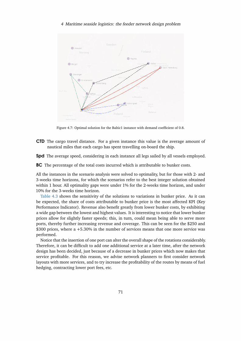
Chapters 2 and 3 deal with two landside problems, namely quay crane assignment andberth allocation; Chapters 4 and 5, on the other hand, tackle two seaside problem: the FeederNetwork Design Problem, a strategic problem asking to find a set of routes for a fleet of vesselswhich maximises the operator’s revenue, and the Travelling Salesman Problem with DraughtLimits, which seeks the optimal route for a single vessel, taking into account that loadingmore cargo in the vessel also increases the amount of draught that it needs in order to enter
2
1 Introduction
a port.
1.1.2 Railway transport
Railway transport involves the movement of people or goods on trains. It is, therefore,usually classified in two macro-areas: passenger rail transport and freight rail transport.Passenger transport is on the rise: Eurostat [15], for example, reports an average increaseof +1.8% passenger-kilometres in 2015 in the European Union, with peak increases of 34%in Slovakia, 18% in Greece, and 15% in Luxembourg. Globally, China, India and Japan leadthe way [35], with a comined total of about 2400 billion passenger-kilometres.
Freight rail transport statistics, however, tell a different story. A trend similar to thatanalysed in Section 1.1.1 for container shipping has emerged in the years following theglobal economic crisis, which has seen the amount of goods shipped by train decrease sharply.Eurostat [15], however, reports that growth in freight rail traffic has now restarted in 12 EUcountries already in 2014, starting with Germany and France (+1.7 billions tonne-kilometres),followed by Romania (+1.4 billions). On the other hand, Finland and Sweden saw a steepcontraction during the same period. In a medium-term perspective, however, rail freight hasgained share in the EU-28 countries, passing from 16.9% of all inland freight transport in2009 to 18.4% in 2014 [14]. Globally, it is the United Stats to lead the league, with their2704 billions tonne-kilometres in 2015, followed by China, Russia, India, and Canada [35].
These numbers show both that rail transport is a crucial part of the global transportationinfrastructure, and that it is increasingly the mean of transport of choice for both passengersand freight. The tranportation of passengers, in particular, involves additional challenges,because a succesfull passenger railway system has stringent requirements in terms of punctu-ality, frequency, connectivity, and resilience. In this thesis we are going to study the problemof rescheduling passenger trains, i.e. of finding appropriate countermeasures when an un-forseen event forces the train operator to depart from its normal operating shedule. This typeof problem is now increasingly studied: so much so that “train rescheduling” has become awell-defined category of optimisation problems. The reader is referred to the excellent surveyby Cacchiani et al. [4] for an overview on train rescheduling algorithms.
1.2 Methodological toolbox
The three main approaches to the solution of a combinatorial optimisation problem consistin using either exact, approximate, or heuristic methods. Exact algorithms provide theguarantee that an optimal solution (if any) to the problem will be found in bounded time.For most interesting problems, however, this bound is often super-polynomial. Classicalcombinatorial problems, such as the Graph Colouring Problem, the Hamiltonian Path Problem,the Minimum Spanning Tree Problem, the Knapsack Problem, the Quadratic AssignmentProblem, are all N P -complete, meaning that the running time of any exact algorithm willgrow at least exponentially with the input size.
For many N P -hard optimisation problems, then, we often have to be content with asolution which is not optimal. Algorithms that produce such solutions are typically classified
3
1 Introduction
as approximate or heuristic. An approximate algorithm is an algorithm that produces asolution of provable minimum quality. This means that a mathematical proof is availablethat the ratio between the value of the solution provided by the algorithm and the value ofthe optimal solution is bounded by a constant (assuming a minimisation problem), calledthe approximation ratio. Measures of quality for these algorithms are, e.g., the ratios in theworst or the average case.
In order to have a proof of the quality produced by an algorithm, we often need suchalgorithm to be simple enough to be studied from a mathematical, combinatorial, geometric,or probabilistic point of view. On the other hand, many well-perofrming non-exact algorithmsfor combinatorial optimisation problems are too complex to be studied in such a way. In thiscase, we talk about heuristic algorithms: they produce solutions with no theoretical qualityguarantee whatsoever, but which are very (or, at least, reasonably) good in practice.
1.2.1 Exact methods
The exact algorithms used to tackle the problems presented in this thesis have, as theirultimate outcome, that of solving a Mixed-Integer Programme (MIP). The most widely usedsuch algorithm is the branch-and-bound algorithm. This algorithm explores the solutionspace by traversing a tree. Each node of the tree represents a more constrained version ofthe original problem and, therefore, has to explore a smaller subset of the solution space.For example, when solving a 0-1 problem, the solution space can be partitioned into twohalves, by considering the two subproblems where the value of a binary variable has beenfixed, repsectively, to 0 and 1. These two subproblems will correspond to two child nodes ofthe root of the tree. By proceeding with further partitioning, the leaves of the tree representsolutions where all variables are fixed to specific values. Exploring the full tree, therefore,would correspond to a complete enumeration of the solution space.
The advantage of using a branch-and-bound algorithm, however, lies precisely in the factthat the whole tree need not be explored. Consider, for example, a bounded 0-1 problem(P01) in minimisation form:
min ct x (1.1)
s.t. Ax � b (1.2)
x 2 {0,1}n (1.3)
Notice that the objective value ct x of a feasible solution x to (P01) always provides an upperbound on the optimal objective value. On the other hand, the optimal solution to a relaxationof (P01) — for example, to its linear relaxation (P01L) — provides a lower bound on theoptimal objective value. During the exploration of a node of the branch-and-bound tree,suppose we have obtained an uper bound UB (e.g. by reaching a leaf, or by means of aheuristic) and, solving (P01L) at the node, we obtain a lower bound LB � UB. Since byfurther constraining the problem, i.e. by fixing more variables, the lower bound producedin the subtree of the current node can only increase, we are confident that we will not findany leaf in such subtree with a better upper bound than the one we already have. For thisreason, we can prune the current node and its whole subtree. Analogously, we can prune thetree when we reach a node where the problem is infeasible.
4
1 Introduction
This algorithm was first proposed by Land and Doig [26] and got its current name whenit was applied to the solution of the Travelling Salesman Problem (TSP) by Little et al. [27].The branch-and-bound method is extremely effective and, therefore, has not only theoreticalbut only practical value, being the underlying algorithm in many commercial MIP solvers.
But another crucial component in the solution of a combinatorial problem is the choice ofthe MIP model used to represent the problem mathematically. Two different MIP formula-tions for the same problem can have dramatically different mathematical and combinatorialproperties (e.g. the strength of the relaxation, the presence of symmetry) that affect howeffectively they can be solved by applying a branch-and-bound algorithm. The most evidentof these properties is arguably the model size. With this respect, we can classify MIP formu-lations into compact and extended. Compact formulations are those for which the size ofthe model is polynomial in the size of input data. By size of the model we mean the sizeof its constraint matrix; e.g. in the case of (P01) this would be the dimension of the spaceto which matrix A belongs. On the other hand, extended formulations are those for whichthe model size is super-polynomial in the size of the input data. We refer the reader to, e.g.,Conforti et al. [8] to a summary of the differences between these two types of formulations.
Branch-and-price
Consider the linear relaxation (P01L) of (P01), and assume we are in the case where (P01L)is bounded and the number of columns of A is exponential in the size of the input. Thismeans that, for a large enough instance of the problem, even inputting (P01L) to a computersolver would take a considerable amount of time, let alone working towards the solution ofthe associated minimisation problem. In other words, even the enumeration of the columnsof A is not viable.
Let K be the set of columns of A 2 Rn⇥m (therefore |K | = m). Consider a smaller subsetK 0 ⇢ K containing only a few of the columns of A, and let (RP01L) be the version of (P01L)where only the columns of K 0 are considered:
minX
k2K 0ck xk (1.4)
s.t.X
k2K 0ahk xk � bh 8h 2 {1, . . . , n} (1.5)
x 2 Rn+ (1.6)
Let x 2 Rn+ be the optimal solution of (RP01L), which we also call the restricted problem, and
let ⇡h � 0 be the dual variables associated with Eq. (1.5) in its �-form. To solve the originalunrestricted programme, we would like to identify which columns in K ✓ K 0 should enterthe base of (RP01L) in order to improve the upper bound. We would then only add thosecolumns, with the hope that we can prove the optimality of (P01L) by moving into K 0 only asmall set of columns from K \ K 0.
Recall from dual theory, that a column missing from the base of the primal problem corre-sponds to a violated inequality in the dual problem. The inequalities in the dual of (RP01L)
5
1 Introduction
are
ck �nX
h=1
ahk⇡h � 0 8k 2 K 0 (1.7)
and therefore, a solution k⇤ 2 K \ K 0 should enter the base iff
c(k⇤) := ck⇤ �nX
h=1
ahk⇤⇡h < 0 (1.8)
where c(k⇤) is called the reduced cost of k⇤. When we can prove that no column in K \K 0 hasnegative reduced cost, again from dual theory, we know that the original unrestricted problem(P01L) has been solved to optimality. In order to have a working algorithm, therefore, wealso need a method to generate new columns with negative reduced cost. Such a method iscalled a pricing algorithm, and is heavily dependent on the nature of the problem we aredealing with. A desirable characteristic of the pricing algorithm is that it is able to find newcolumns with negative reduced cost (or to prove that none exist) in short time, and ideallyin polynomial time.
By solving iteratively the linear relaxation of the reduced problem (also called the masterproblem), and the pricing problem, we obtain an algorithm for the solution of (P01L), whichtakes the name of a column generation algorithm. This method to solve a linear problemwith a potentially exponential number of variables was introduced by Ford and Fulkerson[16] and succesfully employed for the first time by Gilmore and Gomory [17, 18].
When we are interested in solving an integer or mixed-integer programme, we can thenembed the column generation approach within a branch-and-bound algorithm: at each nodeof the tree, the linear relaxation at that node is solved by means of column generation. Such acombined algorithm is called a branch-and-price algorithm. This combination of algorithmsis not straightforward. The main problem lies, in fact, in the effect of branching decisionsto the master and pricing problems. It is well known (see, e.g., Barnhart et al. [2]) that asimple branching rule that fixes the values of the variables in the master problem is oftenproblematic to enforce in the subproblems. In many cases, therefore, alternative branchingstrategies have to be devised, which partition the solution space in ways other than fixingthe variable values. We refer the reader to Lübbecke and Desrosiers [29] and Desrosiers andLübbecke [12] for further introductory material on column generation and branch-and-pricealgorithms.
Branch-and-price algorithms are used in Chapters 3 and 4 to provide exact solutions,respectively, to the Partition Colouring Problem — also used to model a Berth AllocationProblem — and to the Feeder Network Design Problem — arising in maritime seaside logistics.In the first case, the number of columns is explonential, as it is the number of (maximal)stable sets in a graph; in the second case, because each column represents a (feasible) routeof a vessel, i.e. a (feasible) sequencing of port visits.
Branch-and-cut
We now consider the related case in which (P01L) is bounded, but it’s the number of rows ofA to be exponential in the size of the input. We employ a similar approach, and consider only
6
1 Introduction
a subset of row, i.e. a subset N ⇢ {1, . . . , n} of constraints, producing formulation (CP01L):
minX
k2K
ck xk (1.9)
s.t.X
k2K
ahk xk � bh 8h 2 N (1.10)
x 2 Rn+ (1.11)
Since we removed some constraints, (CP01L) is a relaxation of the original problem (P01L).Therefore, if the optimal solution x⇤ to (CP01L) also satisfies the removed constraints, thenit is also the optimal solution for (P01L). Otherwise, we will have to identify which removedconstraint is violated by x⇤; we can then add it to the model, and resolve. This iterativeprocess is commonly called a cutting planes algorithm. The problem of identifying whichimplicit constraint is violated by a solution of (CP01L), or to prove that none are, is namedthe separation problem. As in the case of the pricing problem, we would like the separationproblem to be quick (hopefully polynomial) to solve, and we have the hope that the optimalsolution to (P01L) is found by separating only a small number of constraints. The cuttingplane algorithm was introduced by Kelley [24].
Notice that, in principle, it is also possible to separate inequalities which are not requiredto produce a feasible solution, but are nonetheless valid: the idea that a linear formulationcould be strenghtened by introducing extra constraints was pioneered by Gouonr [22]. Theseextra constraints take the name of valid inequalities and, depending on their number, caneither be added to the original formulation, or separated using a cutting plane algorithm.
When we are solving and integer or mixed-integer programme, similarly to what donefor column generation, we can embed a cutting plane algorithm into the exploration ofthe branch-and-bound tree, thereby using a branch-and-cut algorithm. Notice that thecorrectness of the overall algorithm is guaranteed by separating violated inequalities just forthe integer solutions, but convergence can be accelerated if the separation problem can beused to derive inequalities violated by fractional solutions as well.
In the first implementations (see, e.g., Crowder and Padberg [9], Crowder et al. [10])cutting planes were used only at the root node of the branch-and-bound tree; such approachis now called cut-and-branch. The first actual implementation of a branch-and-cut algorithmwas presented by Padberg and Rinaldi [36] to solve the Travelling Salesman Problem (TSP).We refer the reader to Mitchell [32] for a general overview on branch-and-cut algorithms.
A branch-and-cut algorithm is used in Chapter 5 to solve a variant of the Travelling Sales-man Problem. Inequalities corresponding to subtour elimination constraints are in expo-nential number, as there is one of them for each possible subset of the set of nodes, andare therefore added only when a violated one is found in any optimal solution to the linearrelaxation of the problem. Furthermore, a number of valid inequalities are also separatedand added to the model, in order to strenghten the formulation.
1.2.2 Metaheuristics
Metaheuristics are paradigms used to create heuristic algorithms. In the words of Glover andKochenberger [21],
7
1 Introduction
“Metaheuristics, in their original definition, are solution methods that orchestratean interaction between local improvement procedures and higher level strategiesto create a process capable of escaping from local optima and performing a robustsearch of a solution space. Over time, these methods have also come to includeany procedures that employ strategies for overcoming the trap of local optimalityin complex solution spaces, especially those procedures that utilize one or moreneighborhood structures as a means of defining admissible moves to transitionfrom one solution to another, or to build or destroy solutions in constructive anddestructive processes.”
In this work, in particular, we are going to use a variety of metaheuristic paradigms: TabuSearch (TS, Glover [19, 20]), Reduced Variable Neighbourhod Search (RVNS, Mladenovic[33], Mladenovic and Hansen [34]), Adaptive Large Neighbourhood Search (ALNS, Ropkeand Pisinger [39]).
These three metaheuristics offer three different solutions to the problem highlighted byGlover and Kochenberger: local search improvements lead to find solutions which are localoptima, potentially very far away from the global optimum. A feasible solution x0 is improvedwith local search by considering a neighbourhood N(x0) to explore, and choosing the bestsolution x1 2 N(x0). If the problem involves the minimisation of an objective functionf (x), then x1 can be chosen as x1 = BEST(N(x0)) := arg minx2N(x0){ f (x)}. This procedurecan be iterated by considering x2 = BEST(N(x1)), etc. When we reach a local optimumxk = BEST(N(xk)), the algorithm must then terminate.
The basic idea behind TS is that local optima can be escaped from, by allowing non-improving moves. One could set, for example, xk+1 as any solution in N(xk) taken atrandom, and not necessarily the best one (which would coincide with the local optimumxk). This approach, however, has a clear disadvantage: most of the time we will have thatxk = BEST(N(xk+1)), thereby cycling back to solution xk and never escaping the “valley”surrounding the local optimum. TS proposes to overcome this limitation by introducing ashort-term memory of moves to forbid, thereby placing them in a tabu list. The definition ofmove can be problem-dependent; it is important, however, that forbidding a move achievesthe desired outcome of forbidding the return to a recently-visited local optimum. Since thememory is short-term (not to reduce too much the solution space), we only place a movein the tabu list for a certain limited number of iterations; this number is known as the tabutenure.
The RVNS metaheuristic, on the other hand, aims at escaping from local minima by ex-ploring increasingly larger neighbourhoods. In this case, instead of defining a single neigh-bourhood N(x), we define a succession of them: N1(x), . . . , Nk(x). These neighbourhoodsare nested, i.e. for all points x of the solution space, N1(x) ⇢ N2(x) ⇢ . . . ⇢ Nk(x). Sincethe size of a neighbourhood Nh can become very large as h increases, they are not exploredcompletely but rather sampled. In this work, we only consider one sample from each neigh-bourhood: if the sample provides a better objective value than the current solution, it isaccepted; otherwise, we sample the next (larger) neighbourhood.
ALNS, finally, is rooted in the idea that, when multiple neighbourhoods are available, thesame neighbourhood can be effective for one instance and ineffective for another. Therefore,
8
1 Introduction
the choice of neighbourhood to use in each iteration of the heuristic should depend on its pastperformance during the solution process of the current specific instance. In particular, ALNSneighbourhoods are defined implicitely as Ndr(x) = r(d(x)). d(·) is a destroy method whichtakes a feasible solution as input, and destroys part of it, returning a potentially unfeasibleone; r(·) is a repair method which takes a destroyed solution and repairs it, producing afeasible solution. If each repair method is able to repair solutions destroyed by each destroymethod, then we will have one neighbourhood Ndr for each possible combination of destroyand repair methods. ALNS will then try to evaluate the destroy and repair methods separately,rather than giving an explicit evaluation of the neighbourhood. This is done by defining ascore for each method and increasing it every time the method is involved in the productionof an improving solution, while decreasing it if the solution is worse than the current one. Ateach iteration, then, the methods are selected randomly with a probability proportional totheir score, thus favouring methods which have “behaved well” for the instance at hand.
The roles these metaheuristics play in the present work are many: we use them to generatestarting solutions to exact algorithms, to efficiently explore the solution space of a problem,and we even study their methodological properties without the explicit aim of solving anyparticular problem. TS is used in Chapter 3 to produce initial solutions for the PartitionColouring Problem; however, we show that ALNS produces better results in a shorter time.This result is particularly interesting, because traditionally ALNS has proven effective insolving “rough landscape” problems, such as Vehicle Routing variants: problems where thenumber of possible objective values is very large (essentially of the same order of the numberof solutions). The Partition Colouring Problem, on the other hand, has a very flat landscapewith a few discrete possible values for the objective function, and moving from a solutionto one with a better objective value is difficult. To this end, we employed a new acceptancecriterion (a criterion to decide wether a new solution should be kept or discarded) whichplays well with flat-landscape problems. TS is furthermore used in Chapter 5 to produceinitial solutions to the Travelling Salesman Problem with Draft Limits.
TS and RVNS are also employed in Chapter 6 as two alternative strategies to decide inwhich order the subproblems of a decomposed problem should be solved, keeping in mindthat the solution of a previous subproblem reduces the solution space of the following ones. Inparticular, the problem of rescheduling a set of trains is decomposed train-by-train; schedulingone train marks certain resourced (tracks, platform) as inaccessible for trains scheduledafterwards. The main idea of the algorithm is to produce greedy schedules for each train insequence, and then perturb their order and re-run the greedy algorithm. TS and VNS comeinto play when deciding how the order pertubation should be made, in order to find a goodcompromise between running times (this real-time algorithm should produce a solution inunder 2 seconds) and solution quality.
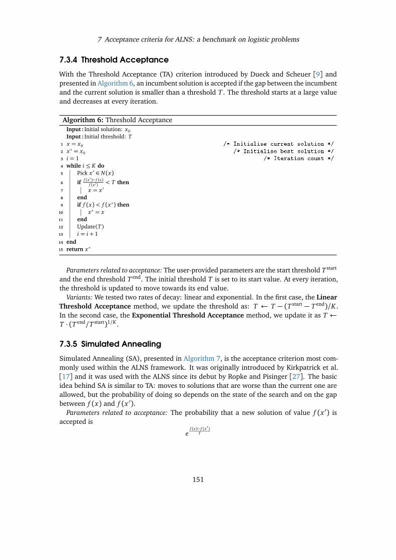
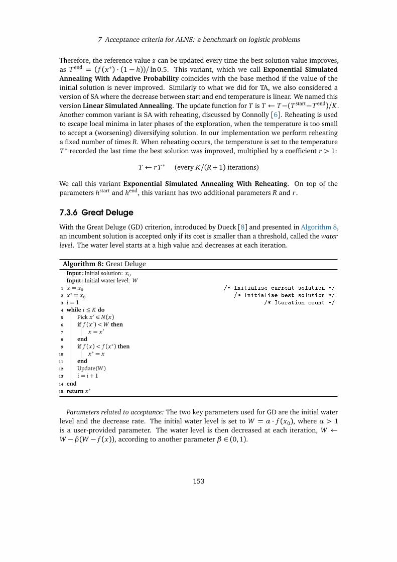
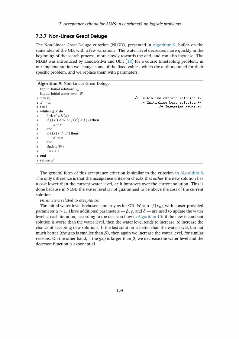
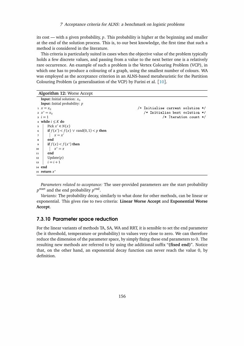
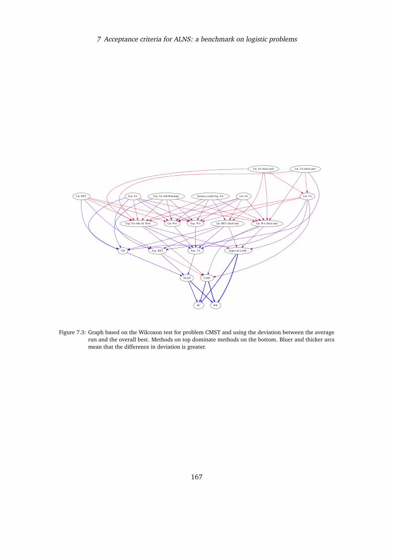
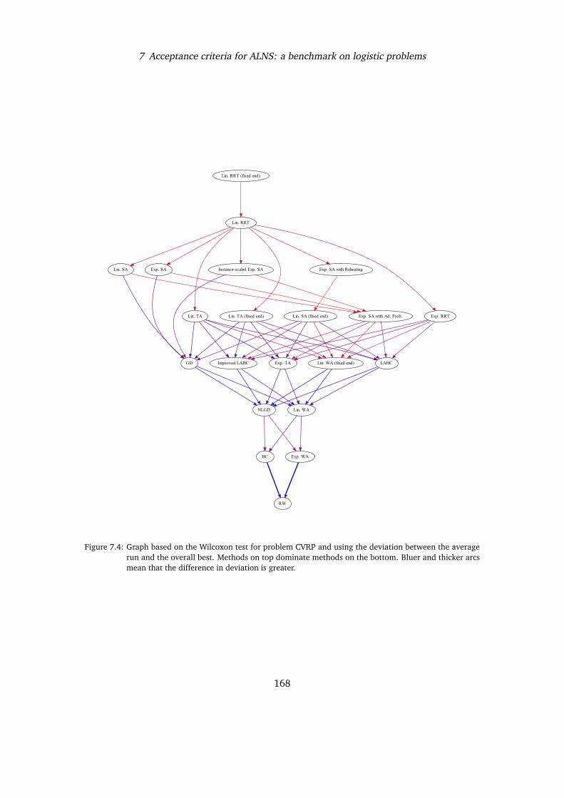
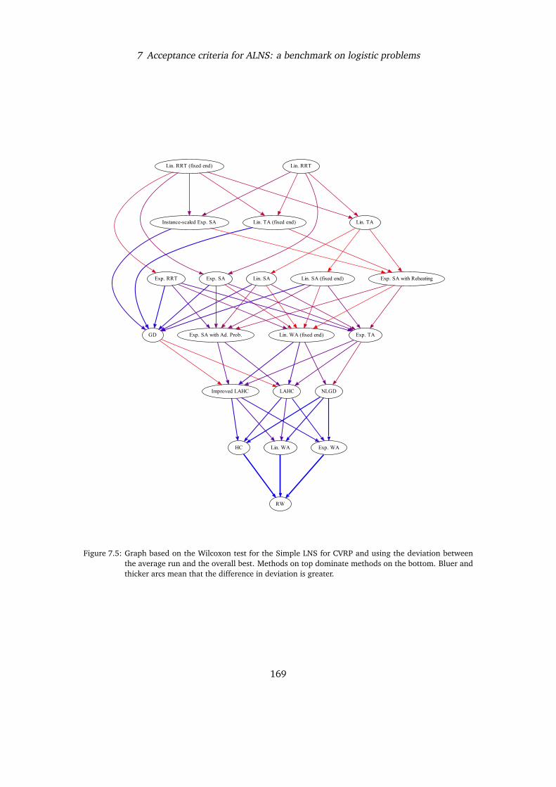
Finally, Chapter 7 investigates the impact of different acceptance criteria on ALNS, andreports results obtained trying the different critera on two relevant optimisation problems:the Capacitated Vehicle Routing Problem, and the Capacitated Minimum Spanning TreeProblem.
9
Bibliography
[1] Regina Asariotis, Hassiba Benamara, Jan Hoffmann, Anila Premti, Vincent Valentine,and Frida Youssef. Review of maritime transport, 2016. Technical report, United NationConference on Trade and Development, 2016.
[2] Cynthia Barnhart, Ellis L Johnson, George L Nemhauser, Martin WP Savelsbergh, andPamela H Vance. Branch-and-price: Column generation for solving huge integer pro-grams. Operations research, 46(3):316–329, 1998.
[3] Christian Bierwirth and Frank Meisel. A survey of berth allocation and quay cranescheduling problems in container terminals. European Journal of Operational Research,202(3):615–627, 2010.
[4] Valentina Cacchiani, Dennis Huisman, Martin Kidd, Leo Kroon, Paolo Toth, Lucas Veelen-turf, and Joris Wagenaar. An overview of recovery models and algorithms for real-timerailway rescheduling. Transportation Research Part B: Methodological, 63:15–37, 2014.
[5] Marielle Christiansen, Kjetil Fagerholt, and David Ronen. Ship routing and scheduling:Status and perspectives. Transportation science, 38(1):1–18, 2004.
[6] Marielle Christiansen, Kjetil Fagerholt, Bjørn Nygreen, and David Ronen. Maritimetransportation. Handbooks in operations research and management science, 14:189–284,2007.
[7] Marielle Christiansen, Kjetil Fagerholt, Bjørn Nygreen, and David Ronen. Ship routingand scheduling in the new millennium. European Journal of Operational Research, 228(3):467–483, 2013.
[8] Michele Conforti, Gérard Cornuéjols, and Giacomo Zambelli. Extended formulationsin combinatorial optimization. 4OR: A Quarterly Journal of Operations Research, 8(1):1–48, 2010.
[9] Harlan Crowder and Manfred W Padberg. Solving large-scale symmetric travellingsalesman problems to optimality. Management Science, 26(5):495–509, 1980.
[10] Harlan Crowder, Ellis L Johnson, and Manfred Padberg. Solving large-scale zero-onelinear programming problems. Operations Research, 31(5):803–834, 1983.
[11] Neil Davidson. Juggling bigger ships, mega-alliances and slower growth, 2016. Termi-nal Operations Conference Europe, Hamburg.
10
Bibliography
[12] Jacques Desrosiers and Marco E Lübbecke. A primer in column generation. In Columngeneration, pages 1–32. Springer, 2005.
[14] Eurostat. Energy, transport and environemtn indicators. Technical report,2016. URL
.
[15] Eurostat. Railway passenger transport statistics: quarterly and annual data 2016.Technical report, 2016.
[16] Lester Randolph Ford and Delbert R Fulkerson. A suggested computation for maximalmulti-commodity network flows. Management Science, 5(1):97–101, 1958.
[17] Paul C Gilmore and Ralph E Gomory. A linear programming approach to the cutting-stock problem. Operations research, 9(6):849–859, 1961.
[18] Paul C Gilmore and Ralph E Gomory. A linear programming approach to the cuttingstock problem – Part II. Operations research, 11(6):863–888, 1963.
[19] Fred Glover. Tabu search — part i. ORSA Journal on computing, 1(3):190–206, 1989.
[20] Fred Glover. Tabu search — part ii. ORSA Journal on computing, 2(1):4–32, 1990.
[21] Fred W Glover and Gary A Kochenberger. Handbook of metaheuristics, volume 57.Springer Science & Business Media, 2006.
[22] RE Gouonr. Outline of an algorithm for integer solutions to linear programs. Bull. Am.Math. Soc, 64:3, 1958.
[23] International Chamber of Shipping. Shipping and world trade, 2017. URL.
[24] James E Kelley, Jr. The cutting-plane method for solving convex programs. Journal ofthe society for Industrial and Applied Mathematics, 8(4):703–712, 1960.
[25] Christos A Kontovas. The green ship routing and scheduling problem (gsrsp): a concep-tual approach. Transportation Research Part D: Transport and Environment, 31:61–69,2014.
[26] Ailsa H Land and Alison G Doig. An automatic method of solving discrete programmingproblems. Econometrica: Journal of the Econometric Society, pages 497–520, 1960.
[27] John DC Little, Katta G Murty, Dura W Sweeney, and Caroline Karel. An algorithm forthe traveling salesman problem. Operations research, 11(6):972–989, 1963.
[28] Lloyd’s Marine Intelligence Unit. Measuring Global Seaborne Trade. Technical report,Lloyd’s, 2009.
[29] Marco E Lübbecke and Jacques Desrosiers. Selected topics in column generation.Operations Research, 53(6):1007–1023, 2005.
[30] Mærsk Line. Mærsk Triple-E, 2017. URL.
[31] MarineTraffic. CSCL Globe, 2017. URL
.
[32] John E Mitchell. Branch-and-cut algorithms for combinatorial optimization problems.Handbook of applied optimization, pages 65–77, 2002.
[33] Nenad Mladenovic. A variable neighborhood algorithm — a new metaheuristic forcombinatorial optimization. In Abstract of papers presented at Optimization Days, page112, 1995.
[34] Nenad Mladenovic and Pierre Hansen. Variable neighborhood search. Computers &operations research, 24(11):1097–1100, 1997.
[35] International Union of Railways. Railways statistics. Technical report, 2016. URL.
[36] Manfred Padberg and Giovanni Rinaldi. Optimization of a 532-city symmetric travelingsalesman problem by branch and cut. Operations Research Letters, 6(1):1–7, 1987.
[37] Photis M Panayides and Dong-Wook Song. Maritime logistics as an emerging discipline.Maritime Policy & Management, 40(3):295–308, 2013.
[38] Harilaos N Psaraftis and Christos A Kontovas. Speed models for energy-efficient mar-itime transportation: A taxonomy and survey. Transportation Research Part C: EmergingTechnologies, 26:331–351, 2013.
[39] Stefan Ropke and David Pisinger. An adaptive large neighborhood search heuristic forthe pickup and delivery problem with time windows. Transportation science, 40(4):455–472, 2006.
[40] Dirk Steenken, Stefan Voß, and Robert Stahlbock. Container terminal operation andoperations research: a classification and literature review. OR spectrum, 26(1):3–49,2004.
[41] Iris FA Vis and Rene De Koster. Transshipment of containers at a container terminal:An overview. European journal of operational research, 147(1):1–16, 2003.
[42] Shuaian Wang, Qiang Meng, and Zhiyuan Liu. Bunker consumption optimizationmethods in shipping: A critical review and extensions. Transportation Research Part E:Logistics and Transportation Review, 53:49–62, 2013.
[43] World Shipping Council. The Liner Shipping Industry and Carbon Emission Policies.Technical report, World Shipping Council, 2009.
2 Maritime landside logistics: the quaycrane assignment problem
Abstract This chapter studies the Quay Crane Scheduling Problem with non-crossingconstraints, which is an operational problem that arises in container ter-minals. An enhancement to a mixed integer programming model for theproblem is proposed and a new class of valid inequalities is introduced. Com-putational results show the effectiveness of these enhancements in solvingthe problem to optimality.
2.1 Introduction
A container terminal manager is faced with several interesting and challenging optimizationproblems and the topic of applying operational research methods to optimize containerterminal operations has received a great amount of attention in recent years. The mostimportant container terminal optimization problems as well as related solution methods aresurveyed by Steenken et al. [7] and Stahlbock and Voß [6].
The focus of this article is on the quay crane scheduling problem (QCSP). In the QCSPa container vessel and a number of quay cranes are given and the objective is to make aschedule for the quay cranes such that the tasks that need to be performed on the vessel arecarried out in a way that satisfies both the terminal manager and the vessel owner. Typicallyit is of primary importance to serve the vessel as quickly as possible. This is in the interestof the terminal manager, as it ensures that valuable quay space is freed up quickly and thatlabor cost is kept in check. It is also in the interest of the vessel owner, because it means thatthe ship can quickly commence its voyage, so to minimize unproductive time.
A conceptual container vessel is displayed in Figure 2.1. The figure shows that storage spaceon the vessel is divided into bays, rows and tiers, with a certain bay–row–tier combinationpointing out a cell in the vessel that can store one forty feet container. This figure is, of course,a simplification. In practice the containers are not stored in a box-shaped vessel, the systemfor numbering positions on the vessel is different from what is used here and containers comein different sizes. The reader is referred to, for example, Pacino et al. [4] for a more realistic
This chapter is based on the contents of: Alberto Santini, Henrik Alsing Friberg, and Stefan Ropke. A note ona model for quay crane scheduling with non-crossing constraints. Engineering Optimization, 47(6):860–865,2015. doi: 10.1080/0305215X.2014.958731.
13
2 Maritime landside logistics: the quay crane assignment problem
description of a container vessel. For the purposes of this work, the simple description issufficient since, as it is common in the QCSP literature, the assumption is made that eachtask consists of unloading and loading an entire bay.
Figure 2.1: Conceptual container vessel
The QCSP model studied in this article is the one presented by Lee and Chen [3] and thecontribution of the article is to show how the model, in a very simple way, can be improved tomake it much more tractable for off-the-shelf solvers like CPLEX. Let B = {1, ..., n} be the setof bays, K = {1, ..., m} the set of quay cranes and pb the processing time of bay b 2 B. Eachcrane can process one bay at a time. Once the processing has started it has to run to its end.Cranes are running on rails, so they cannot overtake each other. The dimensions of bays andcranes are such that it is impossible to place two or more cranes at any bay simultaneously.it must be decided which crane should process which bay and at what time, while respectingthe non-crossing constraint and the necessary time for processing each bay. It is assumed thatthe time for moving the crane between bays is negligible compared to the time for processingeach bay. The objective is to minimize the make-span of the entire operation; that is, tominimise the ending time for the crane that ends the latest.
A classification scheme for QCSP formulations as well as a survey of contributions tothe problem are presented by Bierwirth and Meisel [1]. QCSP formulations are classifiedaccording to four attributes: 1) task attribute, 2) crane attribute, 3) interference attributeand 4) performance attribute. The QCSP studied in this article is classified as “Bay | – | cross| max(compl)” which means that 1) each individual task is a bay — as opposed to a group ofbays or a single container at the two extremes, 2) there are no special attributes associatedwith cranes, 3) the non-crossing of cranes is respected and 4) the maximum completion timeof all tasks is minimized.
14
2 Maritime landside logistics: the quay crane assignment problem
2.2 Mathematical modelThe mathematical model is based on that of Lee and Chen [3] which in turn is an improvedversion of the model presented by Lee et al. [2]. The model uses the binary variable xbkwhich is 1 if and only if bay b 2 B is served by crane k 2 K , the binary variable ybb0 is 1 ifand only if work on bay b 2 B is finished before work on bay b0 2 B starts. The variablescb indicate the completion time of bay b 2 B and c is the overall makespan. Using thesevariables and letting M be a sufficiently large positive integer number, the model is:
xbk = 0 8b 2 B, k 2 K , k > b (2.8)xbk = 0 8b 2 B, k 2 K , n� b < m� k (2.9)xbk 2 {0,1} 8b 2 B, k 2 K (2.10)ybb0 2 {0, 1} 8b, b0 2 B, b 6= b0 (2.11)cb 2 R 8b 2 B (2.12)c 2 R (2.13)
The objective function (2.1) minimizes the total make-span of the process. Constraint (2.2)together with the minimization of the objective function ensures that c is equal to the largestof all completion times. Constraint (2.3) makes sure that the completion time of each bay isgreater than its processing time. Constraint (2.4) ensures that every bay is served by exactlyone crane. Constraint (2.5) links the ybb0 and cb variables. It forces ybb0 to zero whenevercb > cb0 � pb0 , that is, when b0 is started before b finishes. Constraint (2.6) makes sure thatthe cranes do not cross and that each crane is working at one bay at a time. Constraint (2.7)ensures that there is always is enough space between two cranes (e.g. that crane 1 and 3never are servicing two adjacent bays simultaneously). Constraints (2.8) and (2.9) ensurethat no crane is pushed outside the bounds of the ship. This is illustrated in Figure 2.2 thatshows an example with 8 bays and 3 quay cranes. In this example it is only crane 1 that isfeasible for bay one; crane 2 and 3 are not feasible since that would imply that crane 1 ispushed further left and there may not be space for that since another vessel may be mooreddirectly to the left of the current vessel or the vessel may be at the end of the quay. Similarlyit is only crane 2 and 3 that can serve bay 7 since serving it by crane 1 would imply thatcrane 3 is pushed out of bounds. In the example, constraint (2.8) fixes x12, x13 and x23 tozero and thereby ensures that no crane is pushed too far left. Constraint (2.9) fixes x71, x81and x82 to zero implying that no crane is pushed too far right.
15
2 Maritime landside logistics: the quay crane assignment problem
Figure 2.2: Bays and feasible quay cranes
The model is different from that of Lee and Chen [3] in two ways. Lee and Chen [3] createstwo dummy bays and two dummy cranes in order to avoid cranes being pushed out of bounds.The dummy bays are situated at each end of the ship and the dummy cranes are locked toserving the two dummy bays during the entire planning period. As explained earlier, in thismodel the same issue is handled by the variable fixing done in (2.8) and (2.9). This modelingapproach is preferred, as it requires fewer decision variables and constraints, while makingthe model easier to understand as well.
The second difference is that constraint (17) of Lee and Chen [3] has been left out. Usingthe notation introduced earlier, the constraint is
cb +M ybb0 � cb0 � pb0 8b, b0 2 B, b 6= b0
It forces ybb0 to 1 when cb < cb0 � pb0 , that is, when b0 starts after b finishes. Forcing the ybb0
variable to one has no impact on the solution of the model since the only other place whereybb0 occurs is in constraints 2.6 and 2.7 and here a value of one implies that the constraintwill never be binding. The only drawback is that the ybb0 sometimes can have a value 0 inthe final solution when the value logically should be 1, but that is not an issue as the onlyinterest is in the values of the xbk, cb and c variables.
The following simple family of valid inequalities has been introduced and its significantimpact on computing experiments will be later shown:
c �X
b2B
xbkpb 8k 2 K (2.14)
Inequality (2.14) simply forces the overall make-span to be greater than the sum of all theprocessing times of the bays served by the same crane.
2.3 Computational results
The purpose of the computational results is to show the impact of inequality (2.14) whensolving model (2.1) – (2.13). The computational tests were performed using a 2.93 GHzIntel Core i7 model 940 that has 4 cores. The MIP model was solved using CPLEX 12.4 whichwas allowed to use all cores of the computer and was allotted one hour per run. Table 2.1shows results on the 24 instances used by Lee and Chen [3] and compare results with and
16
2 Maritime landside logistics: the quay crane assignment problem
without constraint (2.14), as well as the results reported in [3]. The authors obtained theoriginal data set from Lee and Chen and conducted the experiments using these instances.
The first column in the table reports the instance name, the first number gives the numberof bays while the second gives the number of quay cranes. The next 6 columns report resultsfrom the mathematical model, including constraint (2.14). The first three of these columnsreport the lower and upper bounds when CPLEX terminated and the corresponding gap iscalculated as (UB-LB)/LB · 100%. The next columns report the time spent by CPLEX, where adash indicates that the solver timed out. The last two of the six columns report if the problemwas solved to optimality and the number of branch and bound nodes explored. The followingsix columns show the same information for the model without constraint (2.14). The secondto last column reports the best solution found by Lee and Chen [3]. Values marked withsuperscript “A” were found using CPLEX, while values marked with superscript “B” werefound using a heuristic. The last column reports if the instance was solved to optimality in[3].
A first observation is that the valid inequality has a tremendous impact on the model.Consider for example the first instance. Without the inequality, CPLEX needs about 90 timesas much time and needs to explore around 290 times as many nodes in the branch andbound tree in order to solve it to optimality. CPLEX is able to solve 15 instances to optimalitywhen using the inequality and only 4 instances without the inequality. For the instances thatnone of the models can solve to optimality, the gap is much lower for the model using theinequalities.
When comparing to the results reported by Lee and Chen [3], it can be noticed that eventhe model without the valid inequality is able to solve more instances to optimality. This hasbeen attributed to the fact that the experiment reported in the present work are using a fastercomputer and a more recent version of CPLEX. Lee and Chen [3] used a 3 GHz Pentium IVcomputer and did not report which version of CPLEX they used. The authors do not believethat the fact that they are using slightly fewer variables and constraints in their model has agreat impact on CPLEX’s ability to solve the problem.
The optimal results obtained with the proposed valid inequalities are often substantiallybetter than the heuristic solutions reported in [3] and for most of the instances that were notsolved to optimality, CPLEX is still able to find a better solution than Chen and Lee’s heuristic.On the other hand, their heuristic is much faster and never uses more than 15 seconds.
The heuristic is also able to find a better solution than CPLEX for the largest instances with100 bays. However, no container ship has 100 bays so such an instance is not realistic: oneof the largest container ships currently in operation, Emma Maersk, has approximately 23bays (based on inspection of photos). It is therefore possible to conclude that the enhancedmodel, within one hour, is able to solve most of the realistic sized instances to optimality.
2.4 Conclusions
In this article the quay crane scheduling model proposed by Lee and Chen [3] has beenrevisited. A simple family of inequalities has been introduced and this has been shown tohave a great impact on the ability to solve the model to optimality. Computational results
17
2 Maritime landside logistics: the quay crane assignment problem
Wit
hco
nstr
aint
s(2
.14)
Wit
hout
cons
trai
nts
(2.1
4)Le
ean
dC
hen[3]
Inst
ance
LBU
BG
ap %Ti
me
(s)
Opt
BBN
odes
LBU
BG
ap %Ti
me
(s)
Opt
BBN
odes
Best
Solu
tion
Opt
16-4
726.
072
60.
03.
44
1287
872
6.0
726
0.0
305.
44
3726
726
726A
416
-558
6.0
586
0.0
1.1
452
8858
6.0
586
0.0
8.8
452
274
610A
17-4
741.
074
10.
034
.64
7428
569
8.0
741
6.2
—23
5936
0674
6A
17-5
600.
060
00.
044
.94
7672
160
0.0
600
0.0
330.
54
3435
505
604A
18-4
720.
072
00.
041
.24
8480
168
7.0
720
4.8
—29
2526
9873
7A
18-5
579.
057
90.
035
.94
2685
457
9.0
579
0.0
233.
74
2587
339
595A
19-4
702.
070
20.
025
5.0
431
7052
578.
070
221
.5—
1482
4165
711B
19-5
567.
056
70.
041
4.2
440
4794
542.
056
74.
6—
2170
2526
580A
20-4
925.
092
50.
057
9.4
410
4327
867
9.0
925
36.2
—95
7804
894
9A
20-5
739.
073
90.
027
1.4
432
3089
677.
074
910
.6—
1466
4665
781B
21-4
759.
075
90.
011
51.1
415
1615
354
0.1
759
40.5
—69
5443
980
1B
21-5
612.
061
20.
033
20.3
437
0308
452
4.0
612
16.8
—87
1379
462
2B
22-4
757.
075
70.
012
03.2
420
4291
761
2.0
759
24.0
—68
2079
076
6B
22-5
611.
061
10.
027
15.0
460
9788
854
4.0
611
12.3
—12
1850
2763
6A
23-4
886.
088
60.
019
16.2
421
6828
456
2.0
889
58.2
—53
7112
591
0B
23-5
708.
871
91.
4—
3148
789
546.
971
330
.4—
5754
008
740B
24-4
857.
586
00.
3—
3722
243
600.
086
143
.5—
4996
441
874B
24-5
686.
069
81.
7—
5210
886
525.
769
331
.2—
3865
710
712B
25-4
1083
.510
870.
3—
2085
828
579.
010
8988
.1—
1020
039
1129
B
25-5
866.
887
10.
5—
2651
609
560.
187
756
.6—
2023
905
921B
50-8
998.
310
252.
7—
3573
6942
7.0
1013
137.
2—
6212
010
46B
50-1
079
8.6
830
3.9
—20
4419
448.
083
987
.3—
2396
552
897B
100-
820
64.9
2132
3.2
—31
9813
365.
0—
——
6735
0721
24B
100-
1016
51.9
1757
6.4
—27
5514
345.
4—
——
5618
7317
47B
Tabl
e2.
1:C
ompu
tatio
nalr
esul
ts
18
2 Maritime landside logistics: the quay crane assignment problem
showed that the improved model is able to solve most instances with realistic size to optimality.The authors believe that the model can provide inspiration for further work in this and relatedareas and that the computational results provided can be used as a basis for comparison forfuture heuristics for the problem.
19
Bibliography
[1] C. Bierwirth and F. Meisel. A survey of berth allocation and quay crane schedulingproblems in container terminals. European Journal of Operational Research, 202:615–627, 2010.
[2] D.-H. Lee, H.Q. Wang, and L. Miao. Quay crane scheduling with non-interferenceconstraints in port container terminals. Transportation Research Part E, 44(1):124–135,2008.
[3] Der-Horng Lee and Jiang Hang Chen. An improved approach for quay crane schedulingwith non-crossing constraints. Engineering Optimization, 42(1):1–15, 2010. ISSN0305-215X.
[4] D. Pacino, A. Delgado, R.M. Jensen, and T. Bebbington. Fast generation of near-optimalplans for eco-efficient stowage of large container vessels. Lecture Notes in ComputerScience, 6971:286–301, 2011.
[5] Alberto Santini, Henrik Alsing Friberg, and Stefan Ropke. A note on a model for quaycrane scheduling with non-crossing constraints. Engineering Optimization, 47(6):860–865, 2015. doi: 10.1080/0305215X.2014.958731.
[6] R. Stahlbock and S. Voß. Operations research at container terminals: a literature update.OR Spectrum, 30:1–52, 2008.
[7] D. Steenken, S. Voß, and R. Stahlbock. Container terminal operation and operationsresearch – a classification and literature review. OR Spectrum, 26:3–49, 2004.
20
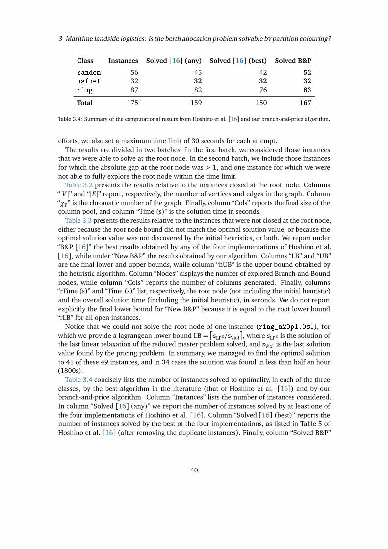
3 Maritime landside logistics: is the berthallocation problem solvable bypartition colouring?
Abstract This chapter presents a study of the Partition Coloring Problem (PCP), ageneralization of the Vertex Coloring Problem where the vertex set is par-titioned, and analyses a claim by Demange et al. [7] that the PCP can beused to solve the Berth Allocation Problem (BAP). The PCP asks to selectone vertex for each subset of the partition in such a way that the chromaticnumber of the induced graph is minimum. We propose a new Integer Lin-ear Programming formulation with an exponential number of variables. Tosolve this formulation to optimality, we design an effective Branch-and-Pricealgorithm. We propose and compare several meta-heuristic algorithms capa-ble of finding excellent quality solutions in short computing time. Extensivecomputational experiments on a benchmark test of instances from the lit-erature show that our Branch-and-Price algorithm, combined with the newmeta-heuristic algorithms, is able to outperform the state-of-the-art exactapproaches for the PCP. After having established that the proposed methodis a suitable tool to solve the PCP, we generated BAP instances, transformedthem into PCP instances, and assessed the feasibility of solving the BAP asa PCP.
3.1 Introduction
Graph coloring problems are among the most studied ones in both graph theory and combina-torial optimization. Given an undirected graph G = (V, E) with |V |= n vertices and |E|= medges, the classical Vertex Coloring Problem (VCP) consists of assigning a color to each vertexof the graph in such a way that two adjacent vertices do not share the same color and thetotal number of colors is minimized. The chromatic number of G, denoted by �(G), is theminimum number of colors in a coloring of G.
This chapter is based on the contents of: Fabio Furini, Enrico Malaguti, and Alberto Santini. Exact and euristicalgorithms for the Partition Colouring Problem. Submitted to Computers & Operations Resarch, pages 1–17,2017.
21
3 Maritime landside logistics: is the berth allocation problem solvable by partition colouring?
The VCP is an N P -hard problem and it has a variety of applications, among which:scheduling, register allocation, seating plan design, timetabling, frequency assignment, sportleague design, and many others (we refer the interested readers to Pardalos et al. [29], Marx[26], Lewis [21]). The VCP and its variants are very challenging from a computational view-point; the best performing exact algorithms are usually based on exponential-size Set Cover-ing formulations, and require Branch-and-Price techniques to be solved (see, e.g., Malagutiet al. [25], Gualandi and Malucelli [13], Held et al. [15], Furini and Malaguti [11]). For densegraphs, good results are obtained by advanced Integer Linear Programming (ILP) compactformulations, like the so-called representatives formulation (see Campêlo et al. [3], Cornazet al. [5]), which are able to remove the symmetry affecting classical descriptive compactILP models.
In this manuscript we study the Partition Coloring Problem (PCP) which is a generalisationof the VCP where the vertex set is partitioned and exactly one vertex of each subset of thepartition has to be colored. The PCP asks to select one vertex for each subset of the partitionin such a way that the chromatic number of the induced graph is minimum. The PCP isN P -hard since it generalizes the VCP and it is also known in the literature as the SelectiveGraph Coloring Problem.
Formally, let P = {P1, . . . , Pk} be a k-partition of the vertex set V of G. A stable set is asubset S ✓ V of non-adjacent vertices, i.e., 8u, v 2 S, uv /2 E. A partial coloring C of G is apartition of a subset of vertices V ⇢ V into h non-empty stable sets or colors (C = {V1, . . . , Vh}),while the remaining vertices V \ V are uncolored. Let f (v) be a function which returns thecolor of a colored vertex v (v 2 V ). The PCP consists of finding a partial coloring C such that:
(i) |V \ Pi |= 1 for i = 1,2, . . . , k;
(ii) f (v) 6= f (w) for all v, w 2 V , vw 2 E;
(iii) h is minimum.
The minimum number of colors used in any optimal PCP solution is denoted in the rest ofthis manuscript as Partition Chromatic Number �P(G,P ).
Let us introduce an example, called Example 1. In the left part of Figure 3.1, we depict agraph G of ten vertices and thirteen edges. The graph is partitioned in five subsets (k = 5),each subset is composed by two vertices; the dotted lines are used to identify the subsets ofthe partition. In the right part of Figure 3.1, we depict a feasible partial coloring C using twocolors (gray and black). For each subset of the partition exactly one vertex is colored. Thecolored vertices, i.e., the vertices v 2 V , are colored with the corresponding color (gray orblack) while the uncolored ones are white.
The PCP models many real-world applications (see Demange et al. [7]) including: routingand wavelength assignment, dichotomy-based constraint encoding, antenna positioning andfrequency assignment, as well as a wide variety of scheduling problems (timetabling, qualitytest) and a variant of the classical Travelling Salesman Problem. Furhtermore, Demangeet al. [7] propose to model the Berth Allocation Problem (BAP) as a PCP, but provide nocomputational evidence on whether this is a practicable solution method for the BAP. Part ofthe aim of the present work is to provide an answer to this question.
22
3 Maritime landside logistics: is the berth allocation problem solvable by partition colouring?
Figure 3.1: Example: (left) a graph G and a partition of its vertices in 5 subsets (k = 5); (right) a feasiblepartition coloring of G with two colors (gray and black).
Figure 3.2: A ship docket at berth 3, occupying berths 3, 4, and 5.
3.1.1 Modelling the Berth Allocation Problem
In the considered version of the BAP (see, e.g., Türkogulları et al. [33]) the terminal operatorhas a list of ships he will have to receive and dock during a certain time horizon. The quayis divided in berths where each ship can dock if the berth, or eventually the adjacent ones(depending on the size of the ship) are not occupied. Figure 3.2 shows a ship docking atberth 3. Because of the ship’s size, no other vessel can use berths 3, 4, and 5 while the shipis docked.
More formally, let U be the set of ships. Each ship is identified by a length lu and an amountof time tu which is needed to load or unload the ship. Let B be the set of berths, alignedalong a quay of total length L. Each berth has a length l b, and starts at a distance db fromthe leftmost point of the quay. The first berth, therefore, will have d1 = 0, the second willhave d2 = l1, the third d3 = l1+ l2, and so on. The time horizon T of duration tmax is dividedinto time intervals, and each ship can dock at a berth b at time interval t if db + lu L andt + tl tmax.
A feasible solution to the problem is an assignment of each ship to a berth and a timeinstant, such that no two ships occupy the same berth at the same time. We will now showhow this problem can be modelled as a PCP on a graph GBAP = (VBAP, EBAP). Consider the
23
3 Maritime landside logistics: is the berth allocation problem solvable by partition colouring?
quay
time
db db + lu
t
t + tu
u
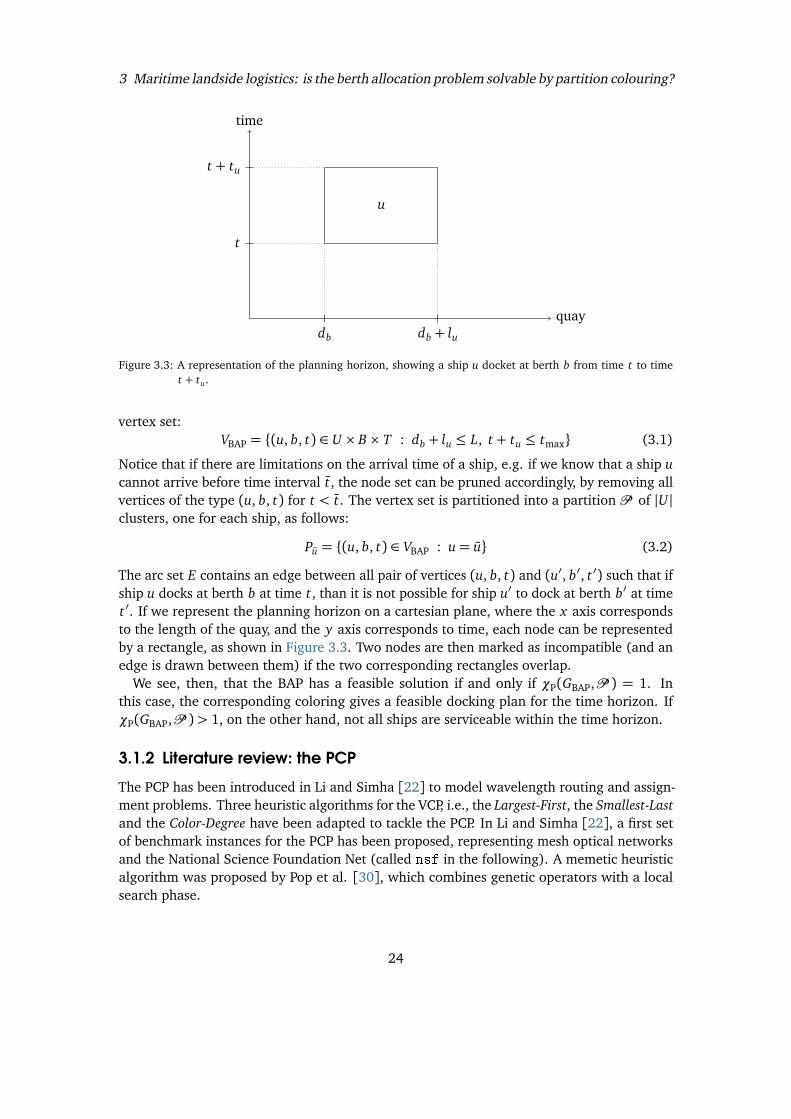
Figure 3.3: A representation of the planning horizon, showing a ship u docket at berth b from time t to timet + tu.
vertex set:VBAP = {(u, b, t) 2 U ⇥ B ⇥ T : db + lu L, t + tu tmax} (3.1)
Notice that if there are limitations on the arrival time of a ship, e.g. if we know that a ship ucannot arrive before time interval t, the node set can be pruned accordingly, by removing allvertices of the type (u, b, t) for t < t. The vertex set is partitioned into a partition P of |U |clusters, one for each ship, as follows:
Pu = {(u, b, t) 2 VBAP : u= u} (3.2)
The arc set E contains an edge between all pair of vertices (u, b, t) and (u0, b0, t 0) such that ifship u docks at berth b at time t, than it is not possible for ship u0 to dock at berth b0 at timet 0. If we represent the planning horizon on a cartesian plane, where the x axis correspondsto the length of the quay, and the y axis corresponds to time, each node can be representedby a rectangle, as shown in Figure 3.3. Two nodes are then marked as incompatible (and anedge is drawn between them) if the two corresponding rectangles overlap.
We see, then, that the BAP has a feasible solution if and only if �P(GBAP,P ) = 1. Inthis case, the corresponding coloring gives a feasible docking plan for the time horizon. If�P(GBAP,P )> 1, on the other hand, not all ships are serviceable within the time horizon.
3.1.2 Literature review: the PCP
The PCP has been introduced in Li and Simha [22] to model wavelength routing and assign-ment problems. Three heuristic algorithms for the VCP, i.e., the Largest-First, the Smallest-Lastand the Color-Degree have been adapted to tackle the PCP. In Li and Simha [22], a first setof benchmark instances for the PCP has been proposed, representing mesh optical networksand the National Science Foundation Net (called in the following). A memetic heuristicalgorithm was proposed by Pop et al. [30], which combines genetic operators with a localsearch phase.
24
3 Maritime landside logistics: is the berth allocation problem solvable by partition colouring?
Theorethical results on the complexity of the PCP on particular classes of graphs have beenobtained in Demange et al. [6] and Demange et al. [8].
To the best of our knowledge, only two works proposed exact algorithms for the PCP: Frotaet al. [10] and Hoshino et al. [16]. The first one proposes a branch-and-cut algorithmbased on the asymmetric representatives formulation introduced by Campêlo et al. [3, 2]for the VCP. A number of valid inequalities are proposed and used within a branch-and-cut framework. A Tabu Search heuristic algorithm has also been proposed to initialize theformulation. Computational tests are reported on randomly generated instances (called
), VCP instances from the literature, and instances derived from the routing andwavelength assignment literature (including the instances, and a new set of instancescalled ).
The second exact algorithm, i.e., the one presented in Hoshino et al. [16], is branch-and-price algorithm based on the Dantzig-Wolfe reformulation of the representatives formulation.In order to deal with an exponential number of variables, a column generation scheme hasbeen proposed which is based on a set of pricing problems, one for each “representative”vertex. The authors show how to adapt to the valid inequalities used by Frota et al. [10] tothe reformulated model. However, since the inequalities did not prove to be computationallyeffective, they were not added to the model. Several heuristic algorithms has also beenproposed in Hoshino et al. [16]. Computational results on the , , andinstances showed that the branch-and-price algorithm of Hoshino et al. [16] outperformsthe branch-and-cut algorithm of Frota et al. [10].
3.1.3 Literature review: the BAP
Many variants of the Berth Allocation Problem exist in the literature. The first distinction ismade between static and dynamic problem. In the static version (see, e.g., Imai et al. [17]),such as the one we consider in this chapter, the ship arrivals are known beforehand to theterminal operator. In the dinamic version (introduced by Imai et al. [18]), on the other hand,this information is only partially known at the initial planning time.
Another distinction is often made relative to the possible docking positions of the ship.Imai et al. [20] consider the case when the position can be chosen arbitrarily along thequayside,and is therefore represented by a real value. The majority of works, however,discretise the berth into segments and impose that each segment can be used by at most oneship at a time (see, e.g., Guan and Cheung [14]).
Finally, a further difference involves the objective function. The BAP can aim to the min-imisation of the total makespan, i.e. the moment at which the last serviced ship is released,or the sum of the waiting times, i.e. the difference between a ship’s arrival and docking times.Finally, if the service time is dependend from the berthing position (notice that our model canhandle this case: the width of the rectangle in Figure 3.3 would then be dependent on thex-coordinate of its left side) a sum of waiting and handling time can be considered [4, 28].Guan and Cheung [14], furthermore, consider a further generalisation of this objective func-tion in which each vessel’s term is multiplied by a different weight. Finally, Imai et al. [19]consider a version of the dynamic BAP in which certain vessels can be given priority overothers. In our work, following the approach proposed by Demange et al. [7] we use a simpler
25
3 Maritime landside logistics: is the berth allocation problem solvable by partition colouring?
approach, as we only study the feasibility of the docking plan, without any considerationrelative to wait or service times.
The BAP has been modelled using variation of other known combinatorial problems. Theparticular case of the discrete version of the problem where each ship only occupies one berthsegment can be modelled as an assignment problem, which can be solved in polynomial timewith the Hungarian method [18]. The more general discrete version can be modelled asan unrelated parallel machine scheduling problem, in both the static and dynamic variants[4]. The continuous version can be modelled as a cutting-stock problem [20]. This is, to thebest of our knolwedge, the first time that the Berth Allocation Problem is solved via graphcoloring.
3.1.4 Paper Contribution
In Section 3.2 we introduce a new formulation for the PCP with an exponential number ofvariables and in Section 3.3 we design a Brach-and-Price algorithm to solve it to provenoptimality. Based on study of the mathematical structures of the formulation, we managedto design a pricing phase based on a unique pricing problem. This is a main improvementwith respect to the state-of-the-art branch-and-price algorithm of Hoshino et al. [16], whichrequires instead to solve several pricing problems, one for each “representative” vertex. In or-der to obtain feasible integer solutions, two different branching strategies are also presentedin Section 3.3. To effectively initialize our branch-and-price algorithm, new meta-heuristicalgorithms are presented in Section 3.4. Several instances of the considered test bed havebeen solved to proven optimality at the root node, i.e., no branching is required, thanks tothe quality of the heuristic solutions and the strength of the lower bound provided by thelinear programming relaxation of the new formulation. In Section 3.5 we present exten-sive computational experiments comparing the new exact and heuristic algorithms with thestate-of-the-art approaches. We also present results relative to the Berth Allocation Probleminstances. Finally, in Section 3.7, we draw some conclusions and depict further possible linesof research on the topic.
3.2 Integer Linear Programming Formulations
In this section we first introduce a natural ILP formulation for the PCP and then we derive anew extended formulation based on the Dantzig-Wolfe reformulation of the natural formula-tion. A trivial upper bound on the number of colors used in any optimal PCP solution is givenby the number k of subsets of the partition. We can then introduce a set of binary variablesy with the following meaning:
yc =
®
1 if color c is used0 otherwise
c = 1,2, . . . , k;
and a set of binary variables x with the following meaning:
xvc =
®
1 if vertex v is colored with color c0 otherwise
v 2 V, c = 1,2, . . . , k.
26
3 Maritime landside logistics: is the berth allocation problem solvable by partition colouring?
The first natural ILP formulation (called ILPN) reads:
(ILPN) minkX
c=1
yc (3.3)
kX
c=1
X
v2Pi
xvc = 1 i = 1,2, . . . , k (3.4)
xvc + xuc yc uv 2 E, c = 1,2, . . . , k (3.5)
xvc 2 {0, 1} v 2 V, c = 1,2, . . . , k (3.6)
yc 2 {0,1} c = 1,2, . . . , k, (3.7)
where the objective function (3.3) minimizes the number of used colors, constraints (3.4)impose that one vertex per subset of the partition is colored, and constraints (3.5) imposethat adjacent vertices do not receive the same color. Finally, constraints (3.6) and (3.7) definethe variables of the formulation.
By replacing constraints (3.6) and (3.7) with
xvc � 0 v 2 V, c = 1,2, . . . , k (3.8)
yc � 0 c = 1,2, . . . , k, (3.9)
we obtain the Linear Programming relaxation of ILPN, that will be denoted as LPN in whatfollows.
Descriptive natural models for coloring problems are known to produce weak linear pro-gramming relaxations and are affected by symmetry (see Malaguti and Toth [23], Cornazet al. [5]), hence, in general they can be solved to optimality only for small graphs. In orderto improve the strength of the linear programming relaxation, and to remove the symmetryof model (3.3)–(3.7), we convexify constraints (3.5) through Dantzing-Wolfe decomposition(see [9]). Let us introduce the following exponential-size collection S of stable sets of Gwhich intersect each subset of the partition at most once:
S = {S ✓ V : uv 62 E, 8u, v 2 S ; |S \ Pi | 1, i = 1, . . . , k} . (3.10)
A valid model for the PCP can be obtained by introducing, for each subset S 2 S , a binaryvariable ⇠S with the following meaning:
⇠S =
®
1 if vertices in S take the same color0 otherwise
S 2 S
then the extended ILP formulation reads as follows:
(ILPE) minX
S2S⇠S (3.11)
X
S2S :|S\Pi |=1
⇠S = 1 i = 1, . . . , k (3.12)
27
3 Maritime landside logistics: is the berth allocation problem solvable by partition colouring?
⇠S 2 {0, 1} S 2 S , (3.13)
where the objective function (3.11) minimizes the number of stable sets (colors), whereasconstraints (3.12) ensure that exactly one vertex of each subset of the partition is colored.Finally constraints (3.13) impose all variables be binary. It is worth noticing that constraint(3.12) can be rewritten as follows:
X
S2S :|S\Pi |=1
⇠S � 1 i = 1, . . . , k, (3.14)
since it is always possible to transform a solution of model (3.11), (3.14) and (3.13) into asolution of model (3.11)–(3.13) of same value. Constraint (3.14) ensures that the associateddual variables take non negative values and this fact helps stabilizing our exact algorithm(see the next section for further details). The resulting formulation (3.11)-(3.14)-(3.13) isdenoted as ILPE in the following.
Finally, by relaxing the integrality of constraints (3.13) to
⇠S � 0 S 2 S , (3.15)
we obtain the Linear Programming relaxation of ILPE, that is denoted as LPE in what follows.By observing that ILPE is obtained by applying Dantzig-Wolfe decomposition of constraints
(3.5) of ILPN and since constraints (3.5) do not form a totally unimodular matrix, it followsthat the quality of the lower bound obtained solving the LP relaxation of ILPN is dominatedby its counterpart associated with ILPE:
Observation 3.2.1. Model ILPE dominates ILPN in terms of Linear Programming relaxation.
Proof. Proving the observation for the specific PCP models give more insight on the structureof the LP relaxation optimal solutions for the ILPN and ILPE models.
We first show that any feasible solution for LPE can be converted to a solution that is feasiblefor LPN. Given a function p(v) which returns the corresponding index i (i = 1,2, . . . , k) ofthe subset of the partition of a vertex v (v 2 V ), we can uniquely define the color c(S) of anyS 2 S as minv2S p(v). Let ⇠⇤ denote a feasible solution to LPE and assume, without loss ofgenerality, that no subset of the partition is covered by more than one selected subset S 2 S .Let us define a solution (x⇤, y⇤) as follows: for each color c set
y⇤c =X
S2S : c=c(S)
⇠⇤S and x⇤vc =X
S2S : c=c(S),v2S
⇠⇤S . (3.16)
Thus, inequalities (3.14) ensure that constraints (3.4) are satisfied. Observe that, by con-struction, for each edge uv 2 E and for each color c = 1,2, . . . , k we have x⇤vc + x⇤uc < y⇤c ;thus, (x⇤, y⇤) is feasible to LPN.
We then show a case where the optimal value of LPE is strictly larger than the optimal valueof LPN. Consider the instance of Figure 3.4, where we depict a graph G of ten vertices andtwenty edges. The graph is partitioned into five subsets (k = 5), and each subset is composed
28
3 Maritime landside logistics: is the berth allocation problem solvable by partition colouring?
by two vertices. As in Figure 3.1, the dotted lines define the subsets of the vertex partition.The figure report also a numbering of the vertices of the graph. The optimal solution of LPE
is ⇠⇤S1= ⇠⇤S2
= ⇠⇤S3= ⇠⇤S4
= ⇠⇤S5= 0.5 where the five stable sets are S1 = {1,8}, S2 = {1,9},
S3 = {2,9}, S4 = {2,10}, and S5 = {8,10}. Thus, the optimal solution value is 2.5, i.e., it islarger than the value of the LP relaxations of LPN, which is 2.
38
2
71
6
5
10
4
9
Figure 3.4: Example: a graph G of 10 vertices and a partition of its vertices in 5 subsets (k = 5).
Model ILPE has exponentially many ⇠S variables (S 2 S ), which cannot be explicitlyenumerated for large-size instances. Column Generation (CG) techniques are then necessaryto efficiently solve ILPE. In the following we present a new Branch-and-Price framework forILPE, and refer the interested reader to [9] for further details on CG.
3.3 A New Branch-and-Price Algorithm
Two are the main ingredients of a Branch-and-Price algorithm, i.e., a CG algorithm to solvethe Linear Programming Relaxation of the exponential-size integer model, and a branchingscheme. We discuss separately these two aspects in the next sections.
3.3.1 Solving the Linear Programming Relaxation of ILPE
Model (3.11), (3.14) and (3.15), initialized with a subset of variables containing a feasiblesolution, is called the Restricted Master Problem (RMP). Additional new variables, needed tosolve LPE to optimality, can be obtained by separating the following dual constraints:
X
i=1,2,...,k :|Pi\S|=1
⇡i 1 S 2 S , (3.17)
where ⇡i (i = 1,2, . . . , k) is the dual variable associated with the i-th constraint (3.14).Accordingly, the CG performs a number of iterations, where violated dual constraints areadded to the RMP in form of primal variables, and the RMP is re-optimized, until no violateddual constraint exist. At each iteration, the so-called Pricing Problem (PP) is solved. This
29
3 Maritime landside logistics: is the berth allocation problem solvable by partition colouring?
problem asks to determine (if any) a stable set S⇤ 2 S for which the associated dual constraint(3.17) is violated, i.e., such that
X
i=1,2,...,k :|Pi\S⇤|=1
⇡⇤i > 1, (3.18)
where ⇡⇤ is the optimal vector of dual variables for the current RMP.At each iteration, the pricing problem can be modeled as a Maximum Weight Stable Set
Problem (MWSSP) on an auxiliary graph G = (V, E), constructed as follows: the vertex set ofG coincides with the vertex set of G while the edge set E is constructed from the edge set ofG and its partition P = {P1, . . . , Pk}:
E = E [ {uv : u, v 2 Pi , i = 1, . . . , k}. (3.19)
In other words, each subset of the partition of G is transformed to a clique in G. Givena weight vector c 2 R|V |+ , where the weight cv of the vertex v 2 Pi is set to the value ⇡⇤iassociated with the i-th subset of the partition, the pricing problem corresponds then to aMWSSP in G, that is, to determine a stable set S of G maximizing
P
v2S cv .Notice that since each partition subset has been turned into a clique, such a stable set con-
tains at most one vertex per subset Pi and therefore collects each profit ⇡i at most once. TheMWSS can be solved by means of a specialized combinatorial Branch-and-Bound algorithm(see Section 3.5).
If a stable set S⇤ has total weight larger than one (that is, the reduced cost is negative),the associated column is added to the RMP and the problem is re-optimized. If, on the otherhand, the total weight is not larger than 1, by linear programming optimality conditions nocolumn can improve the objective function of the RMP and therefore we have solved LPE tooptimality.
3.3.2 Branching scheme for ILPE
The design of a branching scheme is crucial for the performance of a branch-and-price algo-rithm [34]. In the following we describe the branching scheme adopted in our new Branch-and-Price framework. Two are its main properties. Firstly, it is a complete scheme, i.e., itensures that integrality can be imposed in all cases. Secondly, it does not require modifica-tions neither on the master problem nor the pricing algorithm. The latter means that ourbranching does not alter the structure of the pricing problem so that the same algorithm canbe applied during the entire search.
Consider a fractional solution ⇠⇤ to LPE, at a given node of the branching tree, and letS ✓ S be the set of columns in the RMP at the node. We propose a branching schemecomposed of two rules applied in sequence, i.e., when the branching condition for the firstrule fails, the second is applied.
The first branching rule is designed to impose that exactly one vertex is colored for eachsubset. Constraints (3.14) impose that the sum of the values of the variables associated withstables sets intersecting each subset is at least one, but in a fractional solution these stablesets can include different vertices in the same subset of the partition. A given subset Pi has
30
3 Maritime landside logistics: is the berth allocation problem solvable by partition colouring?
more than one (partially) colored vertex if:
|{v 2 Pi :X
S2S ,v2S
⇠⇤S > 0}|> 1 (3.20)
In case more than one such subset exists, we select the subset i with the largest number of(partially) colored vertices, breaking ties by size of the subsets (preferring smaller subsetsand breaking further ties randomly). We then branch on the vertex v 2 Pi with the largestvalue of
P
S2S ,v2S ⇠⇤S . Two children nodes are then created:
• in the first node we impose that v is the colored vertex for subset Pi;
• in the second node, we forbid that v is the colored vertex for subset Pi .
This branching rule can be enforced without any additional constraint neither for the RMPnor for the pricing problem. To force the coloring of v in the children nodes of the branchingscheme, we remove from the graph G all other vertices u 2 Pi (u 6= v); to forbid the coloringof v, we simply remove the vertex from the graph G. This first branching rule is not completesince it may happen that a vertex (partially) belongs to more that one stable set in the solution⇠⇤.
If this happens for a vertex v, there must be another vertex u (belonging to a differentsubset of the partition) such that:
X
S2S :v,u2S
⇠⇤S = �, �is fractional. (3.21)
We say that v and u are a fractionally colored pair of vertices.The second branching rule is designed to impose that each pair of (colored) vertices either
takes the same color, or the two vertices of the pair take different colors. This rule has beenproposed for the VCP by Zykov [35] and used to derive several effective Branch-and-Pricealgorithms for the VCP, starting from the seminal work by Mehrotra and Trick [27], see, e.g.,[25, 13, 15]. In case more pairs of fractionally colored vertices exist, we select the pair v andu with the largest � value. Two children nodes are then created:
• in the first node we force vertices v and u to take the same color;
• in the second node we force vertices v and u to take different colors.
The second branching rule can also be enforced without any additional constraint neither forthe RMP nor for the pricing problem. To force different colors for a pair of vertices v and uin the children nodes of the branching scheme, we add the edge vu to E. On the other hand,to force v and u to take the same color, we remove v and u from the graph G and replacethem with a new vertex z; we add edges zw for all w 2 V such that either uw 2 E or vw 2 E.We then consider a stable set containing the vertex z coloring both Pp(v) and Pp(u), where thefunction p(v) (v 2 V ) returns the index of the subset of the partition containing vertex v.
In our Branch-and-Price algorithm we first define the vertices for each subset of the partitionto be colored, i.e., we apply the first branching rule. Then, in case the solutions are stillfractional, we apply the second branching rule in order to obtain integer solutions.
31
3 Maritime landside logistics: is the berth allocation problem solvable by partition colouring?
After branching, the variables that are incompatible with the branching decision are re-moved from the children nodes. The following observation states that the two proposedbranching rules define a complete branching scheme for the formulation ILPE:
Observation 3.3.1. The two branching rules applied in sequence provide a complete branchingscheme for model ILPE.
Proof. After the application of the first branching rule, the colored vertex in each subset ofthe partition is determined. In [1] it is proved that for any 0-1 constraint matrix A (as for thecase of LPE), if a basic solution ⇠⇤ to A⇠ = 1 is fractional, then there exist two rows i and jsuch that:
0<X
S2S : i, j2S
⇠⇤S < 1 (3.22)
This result allows us to conclude that if a solution is fractional then we can determine twosubsets of the partition such that (3.22) holds. The same holds for the case in which A⇠⇤ > 1:in any optimal fractional solution to LPE, the rows for which covering constraints are satisfiedwith equality must be covered by at least two columns with associated fractional variables,and the previous result applies. By picking the colored vertex from the first and the coloredvertex from the second subset, the two vertices constitute a fractionally colored pair of verticeson which to apply the second branching rule.
3.4 Heuristic algorithms
We devised three algorithms based on meta-heuristics: a Tabu Search, inspired by that ofMalaguti et al. [24]; a heuristic based on the Adaptive Large Neighbourhood Search (ALNS,first introduced by Ropke and Pisinger [31]) heuristic; a variation of the ALNS-based heuristic,improved by a Local Search phase. These algorithms are used to initialize the Branch-and-Bound algorithm with a feasible solution of good quality. Basic initial solutions are providedto the heuristics. They are created by a simple greedy procedure that constructs stable setsone at the time. Starting from a stable set composed by a vertex from an uncolored subset,the procedure keeps adding the least connected vertices of uncolored subsets to the currentstable set. When this is not possible anymore, it starts a new stable set.
3.4.1 Tabu Search
The Tabu Search algorithm aims to find solutions to the PCP that use exactly k colors. Oncesuch a solution has been found, the heuristic is restarted, trying to find a solution of k � 1colors, and so on, until a stopping criterion intervenes.
The algorithm considers k+1 buckets B1, . . . , Bk+1. Each of the first k buckets represents afeasible stable set of S . The (k+ 1)-th bucket contains all other vertices. A feasible solutionis reached when the stable sets B1, . . . , Bk form a selective coloring for the graph G.
At each iteration, we randomly select an uncolored subset Pi and a random vertex v 2 Pi(from Bk+1). We try to insert v in each of the first k buckets and compute a score for each
32
3 Maritime landside logistics: is the berth allocation problem solvable by partition colouring?
insertion, given by the sum of the external degrees of all the vertices that would have toleave Bi , when v enters it. The external degree of a vertex w is the number of vertices u suchthat w, u 2 E and p(w) 6= p(u). After evaluating each possible insertion, we perform the onewhich has the lowest score. Notice that, if there is a bucket i where we can place v withouthaving to remove any other vertex, this insertion has score 0 and is always the preferred one.When inserting vertex v in bucket Bi, we add the couple (i, v) to a tabu list, meaning that,for the next I iterations (where I is a parameter) if v exits bucket Bi , it cannot re-enter it. Inour experiments, we set I = 150; the algorithm was run for 50000 iterations.
3.4.2 ALNS-based heuristic
The basic idea behind ALNS is to explore the solution space using a large collection ofneighbourhoods. At each iteration, the neighbourhood to explore is chosen randomly, with aprobability proportional to a given score. The score, in turn, reflects the past performance ofthe neighbourhood during the solution process. Algorithm 1 shows the general frameworkof ALNS.
In Line 1 and Line 2 the current and best solutions are initialized; Line 3 initializes theiteration counter, and Line 4 initializes the neighbourhood scores. The algorithm is runfor maxiter iterations. At each iteration, a neighbourhood is selected (Line 6) using aroulette-wheel selection mechanism, with probabilities proportional to the scores. Since theneighbourhood size is often exponential, N is often not explored completely, but just sampled,in order to produce a new solution x 0 (Line 7). Next, in Line 8, the new solution is evaluatedand either accepted or rejected, according to an acceptance criterion. The acceptance criterionuses a set of parameters that can change during the solution process: for example, acceptingworsening solutions might be more likely at the beginning of the process than at the end.The current (Line 9) and best (Line 12) solutions are possibly updated, and finally the scores(Line 14), the acceptance criterion parameters (Line 15) and the iteration counter (Line 16)are updated, and the best known solution is returned on Line 18.
In our algorithm, the set N of neighbourhoods is not explicitly enumerated. Rather, wegive a set of destroy methods and a set of repair methods. The former transform a feasiblesolution into an unfeasible one, and the latter transform an unfeasible solution into a feasibleone. Each combination of a destroy method, followed by a repair method gives rise to aneighbourhood. Rather than keeping scores for the neighbourhoods, then, we keep thescores of the individual destroy and repair methods and perform two independent roulette-wheel selections. Notice that this approach can only work if (as in our case) all destroy andrepair methods are compatible, meaning that it is possible to repair a destroyed solutionproduced by any destroy method, with any repair method.
In our implementation, we devised the destroy and repair methods described below. Inorder to compact the exposition, some similar methods have been grouped together and theirdistinctive elements are listed in curly braces.
• Destroy methods
1. Select {a random, the smallest, the biggest} stable set of the solution, and removea random vertex from that set.
33
3 Maritime landside logistics: is the berth allocation problem solvable by partition colouring?
Algorithm 1: ALNS Framework
Input : Initial solution: x0Input :List of neighbourhoods: NInput :Neighbourhood scores: �N for N 2 NInput :Acceptance parameters: pInput :Objective to minimize: f (·)
1 x = x02 x⇤ = x03 i = 14 �N = 1, 8N 2 N
5 while i maxiter do6 Choose neighbourhood N 2 N with probability proportional to �N7 Select x 0 2 N(x)8 if Accept new solution x 0 (using parameters p) then9 x = x 0
10 end11 if f (x)< f (x⇤) then12 x⇤ = x13 end14 Update scores �15 Update acceptance parameters p16 i = i + 117 end18 return x⇤
2. Select the colored vertex with {smallest, largest} external degree, and remove itfrom the stable set it belongs to.
3. Select the colored vertex with {smallest, largest} color degree, and remove it fromthe stable set it belongs to. The color degree of a vertex v is the number of verticesw such that {v, w} 2 E and w is colored in the current solution.
4. As in Items 2 and 3 but the vertex to be removed is chosen with a roulette wheelmethod, in which the probability of being chosen is {directely, inversely} propor-tional to its degree.
5. Select {a random, the smallest} stable set of the solution, remove the stable set.
6. As in Item 5, but the criterion used to choose the set is that it has the smallestcumulative {external, color} degree, defined as the sum of the degrees of itsvertices.
7. As in Item 6, but where the set is chosen with a roulette wheel method, in whichthe probability of being chosen is inversely proportional to the cumulative degree.
• Repair methods
1. For each uncolored subset, select a random vertex from the subset and add it to{a random, the smallest, the largest} feasible stable set of the current solution. If
34
3 Maritime landside logistics: is the berth allocation problem solvable by partition colouring?
it is not possible to put the vertex in any existing stable set, define a new stableset.
2. As in Item 1, but for each uncolored subset, we select the vertex with smallest{external, color} degree.
The scores of the destroy and repair heuristics are updated at each iteration as follows:if a method produced a new best solution, its score is increased by 0.5; otherwise, if amethod produced a solution accepted by the acceptance criterion, its score is increased by0.1; otherwise, its score is reduced by 0.5%.
The classical acceptance criterion used within ALNS is Simulated Annealing, in which asolution is accepted with probability exp(( f (x)� f (x 0))/T ), where T is a parameter (calledtemperature) that decreases exponentially during the solution process. However, the objectivefunction f (·) we consider simply counts the number of used colors, and therefore it onlyassumes a very limited range of discrete values, while moving from one value to the next(i.e., reducing the number of colors by one) is a relatively rare occurence. For these reason,an acceptance criterion that accepts a solution based on its objective value does not seemparticularly suited for the PCP. We, therefore, decided to use the “Worse Accept” criterion,proposed by Santini et al. [32], which accepts a new solution x 0 if either it uses strictly fewercolors than the current one, or otherwise with a certain probability p, which starts at a highvalue, and decreases linearly to reach 0 at the end of the solution process. Notice that p doesnot depend on the value f (x 0) of the new solution. In our implementation, we used the startvalue p = 0.05, and the algorithm was run for 20000 iterations.
3.4.3 Local Search refinement
The local search is a heuristic procedure that can be applied each time a new solution isgenerated by the destroy and repair heuristics, before the solution is evaluated. Althoughapplying the refinement to all generated solutions certainly increases the running time of thealgorithm, it also produces solutions of higher quality, and gives an important improvementon the overall quality of the algorithm, as outlined by the computational experiments reportedin Section 3.5.2.
The local search operator tries to reduce the number of colors used in a solution by one unit,by emptying the smallest cardinality stable set in the solution. Assume the current solutionuses k colors S1, . . . , Sk and, without loss of generality, that Sk is the smallest cardinalitystable set. The local search heuristic first uncolors all vertices of Sk. It then considers eachuncolored partition, and tries to color any vertex (say v) of the partition by inserting it inone of S1, . . . , Sk�1.
If there is a stable set Si such that Si [ {v} is still a stable set, v is placed in Si . Otherwise,the procedure tries to insert v in one stable set Si by removing all vertices w1, . . . , wr in Sithat are not compatible with v, i.e., v, wj 2 E for j = 1, . . . , r. If it is possible to greedilyrelocate all vertices wj in other stable sets, the vertices are relocated, and v is inserted in Si .If there is no stable set where vertex v can be inserted, the procedure tries to color anothervertex from the same uncolored partition. The uncolored partitions, the vertices v from theuncolored partition and stable sets Si and are considered in random order.
35
3 Maritime landside logistics: is the berth allocation problem solvable by partition colouring?
Table 3.1: Quality of the solution produced by Tabu search, ALNS, and ALNS enhanced with local search.
If, for some uncolored partition, no vertex can be inserted in a stable set S1, . . . , Sn�1, localsearch is stopped. On the other hand, if the local search manages to recolor one vertex foreach uncolored partition, it has reduced the number of colors in the solution by one.
3.5 Computational Results: PCP
The experiments have been performed on a computer with a 3.10 GHz 4-core Intel Xeonprocessor and 8Gb RAM, running a 64 bits Linux operating system. The algorithms werecoded in and all the codes were compiled with and optimizations. At eachiteration of the Column Generation procedure (see Section 3.3), we used asa Linear Programming solver (ran single-threaded). The pricing MWSS subproblems weresolved using the open-source implementation of the algorithm described in Held et al. [15]and available at .
3.5.1 Instances
In order to compare our results with the ones present in the literature, we tested our approachon the instance classes , and presented in Section 3.1.2. In their work,Hoshino et al. [16] consider a subset of 187 out of a total of 199 instances, removing thoseinstances solved to optimality in less than a second by either their algorithm or that of Frotaet al. [10].
We, in turn, removed 12 instances of the class, as we realised that they were identicalcopies of the same three basic instances. In particular, instances toall correspond to the same instance (therefore only 1 out of the 5 instances has been kept),as do the analogous instances of base type and . This reduced the total number ofinstances to 175. In particular, we used 56 , 32 , and 87 instances. Wealso note that in instances, all elements of the partition have cardinality 2.
3.5.2 Initial Heuristics
This section compares the three initial heuristics presented in Section 3.4. Out of the 175instances we considered, we know the optimal result (either from our branch-and-pricealgorithm, or from that of Hoshino et al. [16]) of 170 of them. For these instances, we
36
3 Maritime landside logistics: is the berth allocation problem solvable by partition colouring?
Figure 3.5: Running time of the three heuristics, versus instance size (measured in number of vertices of thegraph).
can compute how well the initial heuristics fare, with respect to the optimal solution value.Table 3.1 shows the number of instances for which each of the three heuristics has found: theoptimal solution; a solution with one, two, three or four colors more than the optimum; asolution with at least five colors more than the optimum. The table shows that the ALNS-basedheuristics outperform Tabu search and that the introduction of a local search phase greatlyenhances the effectiveness of ALNS. Figure 3.5 shows computational times for the threeheuristics. Notice that the time axis is logarithmic, showing an exponential dependency ofthe running time to the number of vertices of the graph. For smaller graphs, furthermore, wealso recorded a dependency of the Tabu Search algorithm to the graph density; this explains,for example, the two clusters of points visible in the area relative to graphs with fewerthan 300 vertices. With respect to ALNS, the introduction of local search slightly increasesthe computational time of ALNS, but the improved solution quality definitely justifies theincrease.
3.5.3 Branch-and-price Algorithm
In this section, we report the results obtained by our new branch-and-price algorithm with atime limit of 1 hour. The time limit includes the runtime of the ALNS+LS heuristic, which isused to generate an initial feasible solution.
Since linear relaxation bounds are generally tight, the overall performance of our algo-rithms very much depends on the ability to find good feasible solutions (upper bounds) earlyin the branching tree. Therefore, we solve the restricted master program as an integer modelwith in a subset of the branching nodes aiming at improving the incumbent solutions.Solving these MIP models can be computationally expensive, for this reason we limit theattempts of improving the upper bounds. We solve the MIP associated with the current pool ofcolumns at the root and at all nodes until the pool contains no more than 400 columns. Then,we solve the MIP every 1000th node explored. In order to avoid unnecessary computational
37
3 Maritime landside logistics: is the berth allocation problem solvable by partition colouring?
Instance |V | |E| �P Cols Time (s) Instance |V | |E| �P Cols Time (s)
Table 3.3: Computational results for instances not solved at the root node.
39
3 Maritime landside logistics: is the berth allocation problem solvable by partition colouring?
Class Instances Solved [16] (any) Solved [16] (best) Solved B&P
56 45 42 5232 32 32 3287 82 76 83
Total 175 159 150 167
Table 3.4: Summary of the computational results from Hoshino et al. [16] and our branch-and-price algorithm.
efforts, we also set a maximum time limit of 30 seconds for each attempt.The results are divided in two batches. In the first batch, we considered those instances
that we were able to solve at the root node. In the second batch, we include those instancesfor which the absolute gap at the root node was > 1, and one instance for which we werenot able to fully explore the root node within the time limit.
Table 3.2 presents the results relative to the instances closed at the root node. Columns“|V |” and “|E|” report, respectively, the number of vertices and edges in the graph. Column“�P” is the chromatic number of the graph. Finally, column “Cols” reports the final size of thecolumn pool, and column “Time (s)” is the solution time in seconds.
Table 3.3 presents the results relative to the instances that were not closed at the root node,either because the root node bound did not match the optimal solution value, or because theoptimal solution value was not discovered by the initial heuristics, or both. We report under“B&P [16]” the best results obtained by any of the four implementations of Hoshino et al.[16], while under “New B&P” the results obtained by our algorithm. Columns “LB” and “UB”are the final lower and upper bounds, while column “hUB” is the upper bound obtained bythe heuristic algorithm. Column “Nodes” displays the number of explored Branch-and-Boundnodes, while column “Cols” reports the number of columns generated. Finally, columns“rTime (s)” and “Time (s)” list, respectively, the root node (not including the initial heuristic)and the overall solution time (including the initial heuristic), in seconds. We do not reportexplicitly the final lower bound for “New B&P” because it is equal to the root lower bound“rLB” for all open instances.
Notice that we could not solve the root node of one instance ( ), forwhich we provide a lagrangean lower bound LB=
⌃
zLPE/zViol⌥
, where zLPE is the solution ofthe last linear relaxation of the reduced master problem solved, and zViol is the last solutionvalue found by the pricing problem. In summary, we managed to find the optimal solutionto 41 of these 49 instances, and in 34 cases the solution was found in less than half an hour(1800s).
Table 3.4 concisely lists the number of instances solved to optimality, in each of the threeclasses, by the best algorithm in the literature (that of Hoshino et al. [16]) and by ourbranch-and-price algorithm. Column “Instances” lists the number of instances considered.In column “Solved [16] (any)” we report the number of instances solved by at least one ofthe four implementations of Hoshino et al. [16]. Column “Solved [16] (best)” reports thenumber of instances solved by the best of the four implementations, as listed in Table 5 ofHoshino et al. [16] (after removing the duplicate instances). Finally, column “Solved B&P”
40
3 Maritime landside logistics: is the berth allocation problem solvable by partition colouring?
Table 3.5: Caracteristics of the generated BAP instances.
lists the number of instances solved by our branch-and-price algorithm.
3.6 Computational results: BAP
The same experimental setting used for the PCP has been used for the BAP. Solving the BAP,as noticed in Section 3.1.1, corresponds to solving the decision version of the PCP wherewe are asking whether or not a partitioned graph can be selectively colored with one color.For this reason, when solving the BAP, the algorithm performs an early termination if eitherthe initial constructive heuristic or the ALNS produce a solution with one color; in this case,the decision problem has affirmative answer. On the other hand, if the initial solution usesmultiple colors, the branch-and-price algorithm is started. If during the exploration of thebranch-and-bound tree the lower bound rises above 2.0, however, then the algorithm is againterminated early; in this case, the decision problem has negative answer.
3.6.1 Instances
We generated four set of random instances. The distinctive features of each set are the number|U | of ships (i.e., partitions), the number |B| of berths, and the time horizon length |T |, asthe vertex set is VBAP ✓ U ⇥ B ⇥ T . Table 3.5 reports these value for each instance set. Teninstances were generated in each set, according to the following procedure.
Each berth length was chosen uniformly at random in the interval [2.0,4.0]; the shiplengths were chosen uniformly at random in the interval [1.0, 6.0]. The ship handling timeswere first drawn from the interval [2,6] proportionally to the ship length; successively, anuniform random number was drawn for each ship from the set {�1,0,1} and was addedto the handling time. The arrival time of each ship was chosen uniformly at random in theinterval [0,8] for the instances with a 12-hours time horizon, and [0,18] for those with a24-hours time horizon.
3.6.2 Algorithm
In this section we analyse the results ottained applying the heuristics and the branch-and-price algorithm for the PCP to the BAP instances. As shown in Table 3.6 the resulting graphsare of considerable dimensions with respect to both number of vertices and edges. Instancesof sets BAP1, BAP2, and BAP3 were all solved to optimality by the initial heuristic, givingaffirmative answer (�P = 1) and therefore producing a feasible berth allocation schedule.
41
3 Maritime landside logistics: is the berth allocation problem solvable by partition colouring?
Instances of class BAP4, on the other hand, were much harder to solve. The combination ofthe constructive heuristic and the ALNS algorithm could not complete within the 1-hour timelimit and was, therefore, truncated. For all these instances the heuristic found a colouringusing two colours. In order to test the exact algorithm, this initial solution was fed to thebranch-and-price solver with an additional hour of available computing time. However, inno case the solver was able to explore the root node within the time limit, and therefore theinstances remain open.
From an analysis of the results, we can roughly group BAP instances into two categories:those for which a feasible berthing plan exists and could be found heuristically, and for whicha berthing plan either does not exist or could not be found heuristically. The results seem tohint that there is little hope to solve this latter group of instances within a reasonable timelimit.
We could solve to optimality instances with up to 40 ships and 10 berths. By comparison,Cordeau et al. [4] solved to optimality instances with up to 25 ships and 5 berths over a timehorizon of one week, using a MIP model ran with a two-hour time limit; their objective wasthe minimisation of the total waiting and service time for the ships, considering that it alsodepends on which berth the ship is moored. Guan and Cheung [14] could solve to optmailityinstances with up to 4 vessels using a MIP model, and up to 15 vessels with a Tree Searchalgorithm; the time horizon was of 1 week and the objective function minimised the waitingtimes. Monaco and Sammarra [28] solved instances with up to 30 ships and 7 berths with acompact MIP formulation, minimising the waiting and service times of the ships.
A direct comparison of these result would bare little value, as the objective functions aretremendously different. In general, we can state that — under certain circumstances — itseems feasible to solve the decision version of the BAP, modelling it as a PCP. This is especiallyuseful for highly trafficked ports where a large number of ships need be served in a short time.The other algorithms proposed in the literature generally fail to provide optimal answersin these scenarios, being more useful on sparse instances where fewer vessels arrive over alarger time horizon.
3.7 Conclusions
In this manuscript we have studied the Partition Coloring Problem (PCP), a generalizationof the classical Vertex Coloring Problem with several real world applications in telecommuni-cations and scheduling. For the PCP, we propose a new ILP formulation with an exponentialnumber of variables and a new Branch-and-Price algorithm to effectively tackle it. In orderto obtain good quality feasible solutions in short computational time, we have developed abattery of heuristic algorithms. Thanks to the new exact algorithm, which exploit the heuris-tic solutions in its initialization phase, we were able to solve to proven optimality 167 out of175 PCP instances from the literature. Extensive computational results have proven that thenew Branch-and-Price framework improves on the previous state-of-the-art exact approachesfrom the literature.
We also applied the above algorithm to Berth Allocation Problem (BAP) instances, in orderto assess the feasibility of solving the BAP as a PCP, as proposed by Demange et al. [7]. The
42
3 Maritime landside logistics: is the berth allocation problem solvable by partition colouring?
Table 3.6: Computational results on the Berth Allocation Problem instances.
43
3 Maritime landside logistics: is the berth allocation problem solvable by partition colouring?
problem we consider is in some sense easier than other versions of the BAP from the literature,as we are only asking whether or not it is feasible to assign a set of ships to a set of berths,without taking into consideration the minimisation of waiting times or the total makespan.Under this simplifying assumption, we could solve instances with up to 40 vessels and 10berths.
Finally, as a future research topic, it could be interesting to analyse the performances ofthe PCP model when it is adapted to take into account the classical objective function forthe BAP. Let, for a berth allocation plan S 2 S , ⌧S be the total waiting and service time forthe ships allocated by S. The objective function (3.11) can then be modified in a bi-levelfashion as
P
S2S (tmax + 1+ ⌧S)⇠S in order to first look for a solution which uses just oneberth allocation plan and, in that case, look for the allocation plan which minimises the sumof the waiting and service time for the ships.
3.8 Acknowledgments
The authors thank Stefan Held for making the source code for the MWSS problem availableonline, and Edna Hoshino for providing detailed computational results for the branch-and-price algorithm of [16]. Enrico Malaguti is partially supported by MIUR (Italy), Grant PRIN2015.
44
Bibliography
[1] Cynthia Barnhart, Ellis L. Johnson, George L. Nemhauser, Martin W. P. Savelsbergh,and Pamela H. Vance. Branch-and-price: Column generation for solving huge integerprograms. Operations Research, 46(3):316–329, 1998.
[2] Manoel Campêlo, Ricardo Corrêa, and Yuri Frota. Cliques, holes and the vertex coloringpolytope. Information Processing Letters, 89(4):159–164, 2004.
[3] Manoel Campêlo, Victor A Campos, and Ricardo C Corrêa. On the asymmetric repre-sentatives formulation for the vertex coloring problem. Discrete Applied Mathematics,156(7):1097–1111, 2008.
[4] Jean-François Cordeau, Gilbert Laporte, Pasquale Legato, and Luigi Moccia. Modelsand tabu search heuristics for the berth-allocation problem. Transportation science, 39(4):526–538, 2005.
[5] Denis Cornaz, Fabio Furini, and Enrico Malaguti. Solving coloring problems as maxi-mum weight stable set problems. Discrete Applied Mathematics, 2016. (to appear).
[6] Marc Demange, Jérôme Monnot, Petrica Pop, and Bernard Ries. On the complexityof the selective graph coloring problem in some special classes of graphs. TheoreticalComputer Science, 540:89–102, 2014.
[7] Marc Demange, Tınaz Ekim, Bernard Ries, and Cerasela Tanasescu. On some applica-tions of the selective graph coloring problem. European Journal of Operational Research,240(2):307–314, 2015.
[8] Marc Demange, Tınaz Ekim, and Bernard Ries. On the minimum and maximumselective graph coloring problems in some graph classes. Discrete Applied Mathematics,204:77–89, 2016.
[9] Guy Desaulniers, Jacques Desrosiers, and Marius Solomon, editors. Column generation,volume 5. Springer Science & Business Media, 2006.
[10] Yuri Frota, Nelson Maculan, Thiago F Noronha, and Celso C Ribeiro. A branch-and-cutalgorithm for partition coloring. Networks, 55(3):194–204, 2010.
[11] Fabio Furini and Enrico Malaguti. Exact weighted vertex coloring via branch-and-price.Discrete Optimization, 9(2):130 – 136, 2012. ISSN 1572-5286.
[12] Fabio Furini, Enrico Malaguti, and Alberto Santini. Exact and euristic algorithms forthe Partition Colouring Problem. Submitted to Computers & Operations Resarch, pages1–17, 2017.
45
Bibliography
[13] Stefano Gualandi and Federico Malucelli. Exact solution of graph coloring problemsvia constraint programming and column generation. INFORMS Journal on Computing,24(1):81–100, 2012.
[14] Yongpei Guan and Raymond K Cheung. The berth allocation problem: models andsolution methods. OR Spectrum, 26(1):75–92, 2004.
[15] Stefan Held, William Cook, and Edward Sewell. Maximum-weight stable sets andsafe lower bounds for graph coloring. Mathematical Programming Computation, 4(4):363–381, 2012.
[16] Edna A Hoshino, Yuri A Frota, and Cid C De Souza. A branch-and-price approach forthe partition coloring problem. Operations Research Letters, 39(2):132–137, 2011.
[17] Akio Imai, Ken’Ichiro Nagaiwa, and Chan Weng Tat. Efficient planning of berth alloca-tion for container terminals in asia. Journal of advanced transportation, 31(1):75–94,1997.
[18] Akio Imai, Etsuko Nishimura, and Stratos Papadimitriou. The dynamic berth allocationproblem for a container port. Transportation Research Part B: Methodological, 35(4):401–417, 2001.
[19] Akio Imai, Etsuko Nishimura, and Stratos Papadimitriou. Berth allocation with servicepriority. Transportation Research Part B: Methodological, 37(5):437–457, 2003.
[20] Akio Imai, Xin Sun, Etsuko Nishimura, and Stratos Papadimitriou. Berth allocation ina container port: using a continuous location space approach. Transportation ResearchPart B: Methodological, 39(3):199–221, 2005.
[21] Rhyd MR Lewis. A Guide to Graph Colouring. Springer, 2015.
[22] Guangzhi Li and Rahul Simha. The partition coloring problem and its application towavelength routing and assignment. In Proceedings of the First Workshop on OpticalNetworks, page 1. Citeseer, 2000.
[23] E. Malaguti and P. Toth. A survey on vertex coloring problems. International Transac-tions in Operational Research, 17:1–34, 2010.
[24] Enrico Malaguti, Michele Monaci, and Paolo Toth. A metaheuristic approach for thevertex coloring problem. INFORMS Journal on Computing, 20(2):302–316, 2008.
[25] Enrico Malaguti, Michele Monaci, and Paolo Toth. An exact approach for the vertexcoloring problem. Discrete Optimization, 8(2):174–190, 2011.
[26] Dániel Marx. Graph colouring problems and their applications in scheduling. PeriodicaPolytech., Electr. Eng, 48(1-2):11–16, 2004.
[27] Anuj Mehrotra and Michael A Trick. A column generation approach for graph coloring.informs Journal on Computing, 8(4):344–354, 1996.
46
Bibliography
[28] M Flavia Monaco and Marcello Sammarra. The berth allocation problem: a strongformulation solved by a lagrangean approach. Transportation Science, 41(2):265–280,2007.
[29] Panos M Pardalos, Thelma Mavridou, and Jue Xue. The graph coloring problem: Abibliographic survey. In Panos M Pardalos and Ding-Zhu Du, editors, Handbook ofcombinatorial optimization, pages 1077–1141. Springer, 1998.
[30] Petrica C Pop, Bin Hu, and Günther R Raidl. A memetic algorithm for the partitiongraph coloring problem. In Extended Abstracts of the 14th International Conference onComputer Aided Systems Theory, Gran Canaria, Spain, pages 167–169, 2013.
[31] Stefan Ropke and David Pisinger. An adaptive large neighborhood search heuristic forthe pickup and delivery problem with time windows. Transportation science, 40(4):455–472, 2006.
[32] Alberto Santini, Stefan Ropke, and Lars Magnus Hvattum. A comparison of acceptancecriteria for the adaptive large neighbourhood search metaheuristic. Journal of Heuristics,Submitted, 2016.
[33] Yavuz B Türkogulları, Z Caner Taskın, Necati Aras, and I Kuban Altınel. Optimal berthallocation and time-invariant quay crane assignment in container terminals. EuropeanJournal of Operational Research, 235(1):88–101, 2014.
[34] François Vanderbeck. Branching in branch-and-price: a generic scheme. MathematicalProgramming, 130(2):249–294, 2011. doi: 10.1007/s10107-009-0334-1.
[35] Alexander Aleksandrovich Zykov. On some properties of linear complexes. Matem-aticheskii sbornik, 66(2):163–188, 1949.
47
4 Maritime seaside logistics: the feedernetwork design problem
Abstract In this chapter the design of a container liner shipping feeder network isdecided, by choosing which port to serve during many rotations which startand end at a hub, and can take an arbitrary shape, potentially visiting thehub multiple times during a fixed time horizon. We take into account manyoperational constraints, such as variable speeds and cargo transit times, andaccordingly generated realistic instances, based on the LinerLib benchmarksuite. We solved the problem with a branch-and-price algorithm, which isable to solve most instances to optimality. Furthermore, we performed acomprehensive scenario analysis to evaluate the sensitivity of the solutionsto changes in external conditions and internal policies, and to formulatepractical guidelines for network planners.
4.1 Introduction
Container liner shipping is the main freight transportation service used to move large quan-tities of cargo over long distances. As opposed to tramp shipping, that describes individualships operated to fulfil the transportation requests as they come, and that decide which oneis more convenient for them to accept, liner ships operate along fixed routes and accordingto a published schedule.
According to Lloyd’s [22], 75% of internationally traded goods by volume was transportedby sea in 2008 and this figure is set to increase: it was already an estimated 85% during2013, according to Drewry [17]. Containerised goods account for a relatively small portionof the shipped volume, but their value per volume unit is higher than that of any other kindof goods, and around 52% of maritime commerce by value is shipped in containers.
Furthermore, the environmental impact of moving goods by sea is certainly non-negligible:World Shipping Council [38] estimated that 2.7% of the global greenhouse gas emissions isaccounted by international maritime shipping, and a quarter of this figure is due to containershipping.
This chapter is based on the contents of: Alberto Santini, Stefan Ropke, and Christian E.M. Plum. A branch-and-price approach to the Feeder Network Design Problem. European Journal of Operational Research (underrevision), pages 1–16, 2017.
48
4 Maritime seaside logistics: the feeder network design problem
Figure 4.1: Different types of rotations. Reprinted from Andersen [2] with permission.
These data make clear that the impact of employing OR tools for the optimisation ofliner container vessels operations can yield enormous results in terms of both business andenvironmental value. And yet, operational research methods have not frequently focussedon liner shipping, especially when comparing the amount of literature relevant to this fieldversus other fields of logistics and transportation (see, e.g., Christiansen et al. [11]).
In this paper, we consider the Feeder Network Design Problem (FNDP), which arises whenplanning the routes of liner container vessels in regional feeder networks. Intercontinentalcontainer routes are operated by big vessels (up to 18000 TEU, Twenty-foot Equivalent Units)that only call the main hub ports. These hubs are characterised by an extensive infrastructurethat makes them suitable to operate with enormous quantities of containers and to efficientlyload and unload extremely big vessels. Networks of smaller vessels load the containersdelivered at the hubs and transport them to smaller ports in a particular region. At the sametime, they collect containers at the small ports and unload them at the hubs, where theywill later be shipped to their final destination on the intercontinental routes. In short, linershipping is organised in hub-and-spoke networks. While more than one hub can exist in thesame region, in this work we focus on single-hub feeder networks.
Since liner vessels operate according to a fixed schedule, the operator issues a publictimetable composed by a sequence of port calls together with their day and time. It is clearlyconvenient that such a schedule be periodic, so that each port is called on a certain day ofthe week that does not change. For this reason, the time horizon considered when planningfeeder routes is a multiple of one week.
Due to the nature of the feeder network, moreover, each schedule starts and ends at the hubport (even though it can visit the hub more than once). For this reason, we usually refer tothe route taken by a vessel as a rotation. Rotations are sometimes classified according to theirstructure: Figure 4.1, reprinted from Andersen [2], depicts cycles, pendulum routes, butterflyroutes, and conveyor belts. In our work, we allow the creation of routes with arbitrary shapes,and that visit the hub any number of times within the time horizon. Therefore, all rotationtypes presented in Figure 4.1 are allowed to be constructed, as particular cases of our routes.
The network designer is also faced with the decision of selecting which ports to serve. Theliner company earns revenue for each container it moves at each served port. The companymight also be requested to pay a penalty when not serving a port, if it had contracts inplace with terminal or logistic operators. Another possibility is that the company decides tooutsource the service to another company (for example, by buying capacity on a competitor’s
49
4 Maritime seaside logistics: the feeder network design problem
vessel). As we will show in the following sections, our model is flexible enough to allow foreach of these scenarios.
We assume that both the delivery and pickup demands of a port are determined and knownin advance. In practice, the data we use comes from forecast of future demand, possiblybased on historical observation or on contracts in place. We also assume that, for each port,the network designer has two decisions to make: whether or not to pickup demand at theport, and whether or not to deliver demand to the port (these decisions are independent).Once the decision is made to serve, e.g. the pickup demand at the port, the total amount ofcargo will be picked up in one visit. In other words, we do not allow split pickup and delivery.
The quantity to maximise is the total revenue from served cargoes, minus the cost of therotations and the eventual penalties or outsourcing costs. The cost of rotations includes porttaxes and calling fees and the vessel’s bunker cost, i.e. the cost of the fuel used by the ship.This latter cost is particularly important for two reasons: first, it makes up a considerableshare of an operator expenses, while its price remains very volatile; second, it is greatlyimpacted by the steaming speed of a vessel, with the relationship between the two beingapproximately cubic:
cost(s) =⇣ s
s⇤
⌘3· cost(s⇤)
where s is the steaming speed, cost(s) is the cost incurred to sail for a unit of time at speed s,s⇤ is the design speed, and cost(s⇤) is the cost to sail for a unit of time at the design speed.Both s⇤ and cost(s⇤) are known in advance.
The constraints the operator is faced with are the limited capacity and number of vesselsavailable, the fact that ports observe certain closing time windows (e.g. ports that are closedfor operations at night), that certain goods might have a maximum time span during whichthey can travel (e.g. perishable goods) and that ports have a maximum draught and thereforenot every vessel can enter every port.
In short, the FNDP requires us to come up with certain routes for a fleet of vehicles (vessels,in this case) that abide particular constraints. The problem is, therefore, related to the well-known Vehicle Routing Problem (VRP) and many of its variants: it combines elements ofthe capacitated VRP since each vessel has a maximum container capacity, the VRP with timewindows, the VRP with heterogeneous fleet since each vessel can differ from the others, theVRP with pickups and deliveries since we have a flow of cargo both from and to the hub, themulti-period VRP because the vehicles can get back to the hub multiple times. We refer thereader to the recent book by Toth and Vigo [35] for a comprehensive review of various VRPvariants.
In these variants of the VRP, however, the set of customers to be served is given and noselection need be performed. With this respect, the FNDP is then related to the family ofOrienteering Problems (OP), and in particular to the multi-vehicle variants which ares presentin the literature under various names, including Team Orienteering Problem (TOP), VRPwith Profit Collection, or VRP with Customer Selection. The TOP has received considerableattention in the recent years (see, for a review, Archetti et al. [4]). While exact algorithmsbased on branch-and-price exist for the TOP [7] and for its capacitated version [3], to thebest of our knowledge no exact algorithm has been developed for cases which include timewindows, or a pickup-and-delivery component.
50
4 Maritime seaside logistics: the feeder network design problem
The main contributions of this paper are three-fold. First, we introduce a mathematicalmodel and an extended formulation for the Feeder Network Design Problem, taking intoaccount the principal real-life constraints that container vessel operators have to face. Second,we provide a state-of-the-art algorithm, which is able to solve to optimality (or with very smallgaps) realistic instances. Third, we perform a wide variety of scenario analyses, from whichwe dystill general principles an operator can apply at the strategic, tactical, and operationallevels.
4.2 Literature review
In this section we summarise recent literature on two important aspects of maritime optimi-sation: liner network design, and speed optimisation. For more general reviews of researchin maritime optimisation, we refer the reader to Christiansen et al. [11], Christiansen et al.[12] and Christiansen et al. [13].
Liner network design
An introduction to liner shipping is given in Brouer et al. [8], where the authors also presenta benchmark model for LinerLib (see Løfstedt et al. [23]), the main instance library usedfor liner shipping problems. The benchmark model for the Liner Network Design Problem(LNDP), is solved by means of a heuristic based on Tabu search and column generation. Abroad introduction to operational research methods in container liner shipping is given inthe survey by Meng et al. [25].
A heuristic, a column generation algorithm and a Benders decomposition algorithm, allcoupled with an iterative search routine, are presented by Agarwal and Ergun [1] to solvethe combined ship scheduling and cargo routing problem, with weekly frequencies and tran-shipments. The authors allow multiple visits to the same port (as long as they happen indifferent days of the week), but do not consider transhipment costs. They test their approachon instances with at most 20 ports and 100 ships.
An exact method is presented by Reinhardt and Pisinger [31] to solve the network designand fleet assignment problem. The authors use a branch-and-cut algorithm to solve instancesup to 15 ports, while considering transhipments, a heterogeneous fleet and allowing butterflyroutes.
Mulder and Dekker [26] propose a heuristic approach to the combined problem of fleetdesign, ship scheduling and cargo routing. The authors first cluster ports by proximity andthen design a hub-and-spoke hierarchy, in which each cluster is served by a feeder network.They test their approach on the Asia-Europe trade lane, comprising 58 ports.
Plum et al. [28] propose to switch the classic arc-flow formulation for the LNDP, with aservice-flow based formulation. Similarly to our work, they consider the Baltic and WesternAfrican scenarios of the LinerLib and propose a mixed-integer linear formulation to maximisethe operator’s profit, under a weekly frequency constraint and allowing multiple calls to thesame port (thereby allowing an arbitrary number of butterfly ports). The model is solvedwith a commercial solver.
51
4 Maritime seaside logistics: the feeder network design problem
Criterion Value Criterion Value
Optimisation Criterion Profit Shipping Market LinerDecision maker Owner Explicit fuel price YesFreight rate Yes Fuel consumption CubicLeg-by-leg optimal speed Yes Speed function of payload NoLogistical context Pickup and delivery Size of fleet Multiple shipsMore ships an option Yes Inventory costs NoModal split No Ports included Yes
Table 4.1: Classification of the present paper under the taxonomy proposed by Psaraftis and Kontovas [29].
Another heuristic method, based on column generation, for the network design and cargoflow problem in liner shipping is presented by Wang and Meng [37]. The authors apply thecolumn generation algorithm to a mixed-integer non-linear non-convex formulation, whichmodels weekly services and maximum transit times (which they refer to as deadlines). Theytest their approach on the Asia-Europe trade lane, considering 12 ports.
Plum et al. [27] presents arc-flow and path-flow models for the single-vessel liner ship-ping service design, in which an operator has to optimise the best-paying demand (pickupsand deliveries) for a round-trip route operated by a single vessel, taking into account maxi-mum transit times. The authors propose a branch-and-cut algorithm, which is able to solveinstances with up to 25 ports.
Speed optimisation
A general review and a taxonomy of existing literature related to speed optimisation forefficient and green maritime transportation is given in Psaraftis and Kontovas [29]. Table 4.1shows the classification of our work under the proposed taxonomy.
Chang and Wang [10] and Cariou [9] study the economical impact and sustainability of slowsteaming in liner shipping. In the first work, the authors conclude that speed optimisation isbest employed as a dynamic process, which depends on both charter rates and fuel prices. Inthe second work, the author concludes that slow steaming is a long-term sustainable strategyon main container trade lanes, if the bunker price is at least $350-$400.
More details on the relation between sailing speed, incurred costs and emissions is givenin Psaraftis and Kontovas [30] and Kontovas [21], in which the authors study the trade-offsinvolved in speed optimisation in broader shipping scenarios. In particular, Psaraftis andKontovas [30] consider many real-life factors impacting on the relationship between speedand costs, stressing the importance of considering hotel costs to adjust the purely cubic costfunction, the dependency of the cost function on the payload, the impact of external eventssuch as weather conditions, and of the maintenance state of the ship (e.g. hull condition).They also mention the importance of en route inventory costs, which clearly tend to increaseat lower speeds on long-distance routes. Kontovas [21], on the other hand, focuses on therelationship between fuel consumption and CO2 emissions.
The work of Wang and Meng [36] studies the leg-by-leg optimisation of sailing speeds,once the routes have already been fixed. The author consider transhipments and container
52
4 Maritime seaside logistics: the feeder network design problem
routing, and propose a Mixed-integer non-linear convex model, for which they give an outerapproximation scheme. They test their approach on an instance with 46 ports and 11 fixedroutes.
4.3 Model
The time in the planning horizon is divided into m time intervals, and it is modelled by the setT = {1, . . . , m}. The size of this discretisation depends on the size of the region considered.As mentioned in Section 4.1, it is convenient that the time horizon be a multiple of one week.If, for example, we consider one month as planning horizon, we can then deploy four shipson each rotation spacing them out by one week, so that each port is visited weekly.
Let n 2 N be the number of ports in the region, excluding the hub. We model each porttwice, once as a pickup and once as a delivery port. The set of all ports is denoted byP 0 = {0,1, . . . , n, n + 1, . . . , 2n} where 0 represents the hub, P� = {1, . . . , n} is the set ofdelivery ports, and P+ = {n+ 1, . . . , 2n} is the set of pickup ports. Ports i and n+ i representthe same physical port.
We also define the set P = P 0 \ {0} of all ports excluding the hub. Each port i 2 P� hasa delivery demand di � 0 and each port j 2 P+ has a pickup demand pj � 0. Furthermore,each port has a maximum draught mp
i > 0, meaning that vessels with a draught greater thanmp
i cannot enter the port. Each port has a handling time hi � 0, that is the number of timeintervals needed to load (if i 2 P+) or unload (if i 2 P�) containers at that port. Since thequantity of containers to be moved at each port is known in advance, an accurate estimateof hi can be given for each port. We assume that when the vessel visits the hub, its handlingtime h0 can be estimated only based on the vessel type, independently from the quantity ofcargo it carries.
Each port has a number of closing time windows which can be used not only to modeltimes at which the port is closed, but also for many other purposes. Here we give a coupleof examples.
• If i is a pickup port that receives most fo the goods it exports (for example, via a freighttrain) at a certain time t0 > 1, then i can be marked as closed until a time t1 � t0 atwhich we can assume the goods are ready to be loaded onto a ship.
• If we use a time horizon representing 2 weeks, and have a delivery port j which isserved weekly by a freight train (at times t0, t1), and which imports perishable goodsthat can stay in the yard at most t 0 time units before they are loaded on the train, we canmark the port as open only during time windows [t0� t 0, t0] and [t1� t 0, t1]. A rotationwill visit j, for example, during the first time window; the second ship deployed onthe same rotation will visit it during the second time window, thereby guaranteeing aweekly visit, and that the goods are not spoiled by staying too long in the yard.
For every pair of ports i, j we have a symmetric distance �i, j � 0. The distances satisfy thetriangle inequality, and are zero for elements modelling the same port, i.e. �i,i = 0 for alli 2 P 0, and �i,n+i = 0 for all i 2 P�.
53
4 Maritime seaside logistics: the feeder network design problem
Hub
Port 1
Port 2
(a) Configuration of the instance, with the ports in their geographical positions.
Hub
Port 1 Pickup
Port 1 DeliveryPort 2 Pickup
Port 2 Delivery
(b) In this graph, the ports have been duplicated (for pickup and delivery) and arcs represent the possibility tosail from one port to another.
Hub
Port 1 Pickup
Port 1 Delivery
Port 2 Pickup
Port 2 Delivery
t = 0 1 2 3 4 · · · m
• • • • • • •
• • • • • • •
• • • • • • •
• • • • • • •
• • • • • • •(c) The time-expanded graph for a particular vessel, where each node is copied once for each time instant. Two
arcs are depicted, representing sailing between two ports at different speeds.
Figure 4.2: Modelling of a simple instance, with one hub and two ports.
54
4 Maritime seaside logistics: the feeder network design problem
We deal with a heterogeneous fleet of k vessels, modelled by set V = {1, . . . , k}. Each vesselv has a capacity Qv > 0 and a draught mv
v > 0. We consider the draught of a vessel as fixed,even though in reality it can change slightly with the amount of load a vessel is carrying.We refer the reader to, e.g., Glomvik Rakke et al. [19], Battarra et al. [6], Malaguti et al.[24] for recent works on maritime routing under draught limits. Each vessel v has a set ofpossible sailing speeds ⌦v = {!v
1, . . . ,!vsv} expressed in nautical miles per discrete time unit
(i.e., the speed is expressed in multiple of knots); sv 2 N is the number of speeds associatedwith vessel v.
We take into account the following cost components:
• Time charter cost: a fixed daily cost that the operator pays to charter the vessel. Weassociate to each vessel v the time charter cost � TC
v (in dollars per time interval).
• Hotel cost: the cost incurred when keeping a vessel moored, but operational. Wedenote the hotel cost for vessel v as �H
v (in dollars per time interval).
• Bunker cost: the sailing cost, which depends on the cruising speed of the vessel. Givena vessel v and a sailing speed !v
k 2 ⌦v , we consider the associated cost � Bvk (in dollars
per time interval).
• Movement costs: the unit costs relative to the handling of the cargo at a port. Given avessel v and a port i, since we know the quantity of cargo that needs to be handled ini, we can compute the total movement cost and denote it as �M
vi (in dollars).
• Fixed port call fee: a flat cost to pay when any vessel calls a port i. This is denoted as� PF
i (in dollars).
• Variable port call fee: a cost to pay when calling a port, but dependent on the capacityof the vessel. A vessel v calling port i will pay � PV
vi (in dollars).
Serving requests generates revenue, as the operator earns a certain fee per Forty-Foot Equiv-alent Unit (FFE) picked up or delivered. The revenue is, for commercial reasons, not uniformand delivering an FFE to a certain port could earn more or less than delivering to anotherport. Therefore, we associate to each port i a revenue Ri > 0 (in dollars) which expressthe total earned by the operator when a vessel serves the port. Analogously, we associate apenalty ↵i � 0 (in dollars) to be paid by the shipping operator if it decides to skip service atthe port. This penalty can be also used to model the cost of outsourcing the service.
Figure 4.2a shows a simple instance of the problem, with one hub and two ports. InFigure 4.2b we create one node for each element of P 0 and draw solid arcs to represent thata ship can sail from any port to any other port. The dotted arcs represent a ship that, at thesame port, first performs a delivery and then a pickup.
4.3.1 Graphs
For each vessel v we create a space-time graph Gv = (N , Av). The node set is common to allgraphs and is defined as N = {�,⌧}[ P 0 ⇥ T where � and ⌧ are, respectively, a source and
55
4 Maritime seaside logistics: the feeder network design problem
sink node. All other nodes (i, t) represent a port at a specific time instant; Gv is, therefore, atime-expanded graph. The arcs Av can be partitioned in four sets:
• Starting arcs of type (�, (0, t)), that link the source node with a node representing thehub.
• Ending arcs of type ((0, t),⌧), that link a node representing the hub with the sink node.
• Delivery-to-pickup arcs of type ((i, t), (i + n, t 0)), that link the delivery and pickupoperations at the same physical port.
• Sailing arcs of the type ((i, t), ( j, t 0)), with j 6= i+n if i, j 2 P, that represent the sailingfrom port i 2 P 0 to port j 2 P 0.
The time used for the operations at the destination node of the arc is precomputed andincluded in the arc itself. To understand how this is done, consider the example of a sailingarc from port i 2 P to port j 2 P, modelling the sailing of vessel v 2 V , starting at time tand sailing at speed !v
k 2 ⌦v. Assume that the draught limits are respected (mpi � mv
v andmp
j � mvv), that i is open at time t, and that visiting j immediately after i does not violate
capacity constraints (pi + pj < Qv if i, j 2 P+, di + dj < Qv if i, j 2 P�, pi + dj < Qv ifi 2 P+, j 2 P�). If these conditions do not hold, then the arc is not created.
The arrival time instant of vessel v will be tarr = t +�i j/!vk. Let t 0 be the time instant in
which the handling operations at j can be completed; if tarr corresponds to a time when portj is open, then t 0 = tarr+hj , otherwise a waiting time has to be factored in, as the ship cannotberth or be operated on, while the port is closed. We can then create the arc ((i, t), ( j, t 0)).
This process is repeated for each pair of ports, for each vessel v 2 V , and for each speed! 2 ⌦v . The delivery-to-pickup arcs are created similarly, while the starting and ending arcsare created for all nodes representing the hub. A starting arc of type (�, (0, t))means that thevessel is leaving the hub at time t and therefore has been waiting idly at the hub during thetime period [0, t]. Analogously, an ending arc of type ((0, t),⌧) represents a ship concludingits rotation at time t and waiting idly during time period [t + 1, m].
Notice that all costs, as well as the revenue, can be modelled on the arcs. For example, thecost of a sailing arc a = ((i, t), ( j, t 0)) is set to:
ca = � TCv (t
0 � t) + �Hv (t
0 � tarr) + � Bvk(tarr � t) + �M
v j + �PFj + �
PVv j � Rj (4.1)
Figure 4.2c shows the time-expanded version of the graph depicted in Figure 4.2b, for aparticular vessel (for simplicity, we omit vertices �,⌧). In the figure, we only draw two arcs:they represent a ship sailing from “Port 1 Pickup” to “Port 2 Pickup”. We can imagine, forexample, that the first arc represents the ship leaving Port 1 at time 1, arriving at Port 2 attime 2, and finishing the loading operations at time 3. The second arc again models leavingPort 1 at time 1 but, sailing more slowly, Port 2 is reached only at time 3, and the loadingoperations are completed at time 4.
56
4 Maritime seaside logistics: the feeder network design problem
4.3.2 Integer formulation
We define a route for vessel v as a succession of consecutive arcs in Av such that the firststarts at � and the last ends at node ⌧. If every port i 2 P is visited at most once, and if thecapacity constraint is not violated, we say that the route is feasible. The set of feasible routesfor vessel v is denoted as Rv and the set of all feasible routes as R=
S
v2V Rv . Notice that itis possible to assign naturally a cost cr to each route r by summing the costs of the arcs thatcompose the route. Finally, let "ri 2 {0, 1} be a parameter with value 1 iff port i is visited byroute r. We can formulate a model for the FNDP by considering binary variables xr takingvalue 1 iff route r 2 R is part of the solution:
(MP) minX
r2R
cr xr +X
i2P
↵i
Ç
1�X
r2R
"ri xr
å
(4.2)
s.t.X
r2R
"ri xr 1 8i 2 P (4.3)
X
r2Rv
xr 1 8v 2 V (4.4)
xr 2 {0,1} 8r 2 R (4.5)
The objective function (4.2) minimises the total cost of selected routes and the penalties paid.(A solution yelds a profit if the value of the objective function is negative.) Constraint (4.3)ensures that each port is visited by at most one vessel, constraint (4.4) guarantees that wedo not use more vessels than available, and finally constraint (4.5) specifies the variables’domain. Notice that, unlike problems in the VRP family, where the requirement that allcustomers need be served leads to set-covering �-constraints, our model has -constraintsin (4.3).
Problem (MP) is called the master problem. An obvious drawback of (MP) is that sets Rv istoo large to enumerate in practice, since the number of feasible routes grows exponentiallywith the size of the graphs. We then consider a version of (MP) where the sets Rv aresubstituted with much smaller sets R0v; this new problem is called the restricted master problem(RMP). The idea behind the branch-and-price algorithm we propose is to solve (RMP) bybranch-and-bound: at each node the linear relaxation of (RMP) is solved and new columnsare added to R0v. In order to find promising columns to add, we solve a pricing subproblem(SP)v for each vessel v, that will produce new columns with negative reduced cost. Fromdual theory, we know that columns with negative reduced cost entering the base will improvethe objective function of the relaxed (RMP). A node is considered explored when it is notpossible to find any negative reduced cost column. Let ⇡i � 0 be the dual variables of (4.3)and µv � 0 be the dual variables of (4.4). Notice that the objective function can be rewrittenas
X
r2R
Ç
cr �X
i2P
↵i"ri
å
xr +X
i2P
↵i (4.6)
and the last sum is a constant. Therefore, the dual cost of a column corresponding to route
57
4 Maritime seaside logistics: the feeder network design problem
r 2 Rv is:cr = cr +
X
i2P
(⇡i �↵i)"ri +µv (4.7)
The dual cost is given by the original route cost; then, for each visited port i 2 P, the dualprice ⇡i is added and the corresponding penalty ↵i is removed; finally, a dual price µv is paid,only depending on the used vessel v 2 V .
4.4 Solution of the pricing subproblem
The pricing subproblem (SP)v is a shortest path problem with resource constraints (SPPRC),as routes for vessel v are paths in Gv from the source node � to the sink node ⌧, and theresource constraints are used to ensure the routes’ feasibility. In some sense, this problem canalso be seen as an elementary SPPRC (ESPPRC). Graphs Gv are acyclic, and therefore anypath would be elementary. In our case, however, we require that every port i 2 P is visited atmost once, i.e. that every subset of nodes Ni = {(i, t) | t 2 T} has at most one inbound andone outbound arc. In the rest of this paper we will refer to this property when we speak ofelementariness.
Notice that the elementariness requirement can be dropped, and routes that visit the sameport multiple times can be generated, as long as the corresponding columns are then removedby suitable branching rules in the master problem (as we will explain in Section 4.5.3). Forthis reason, in this section we propose algorithms to solve both the ESPPRC and the SPPRC.
4.4.1 Greedy-randomised heuristic for the ESPPRC
We can attempt to find negative-reduced-cost elementary path with a simple greedy algorithmthat builds a path starting in � and then proceeds by choosing one random arc among theK1 outgoing arcs of least reduced cost that do not close a cycle, until ⌧ is reached. Thesame procedure can also be applied backward, starting in ⌧ and ending at �. After the pathis constructed, we can check that the capacity constraint has not been violated by a singlepass over the list of visited ports; if the path is not capacity-feasible, or if its reduced cost isnon-negative, it is discarded. The algorithm can be applied in both directions many times,as its computational time is very small, thereby increasing the chances that a feasible pathof negative reduced cost is found.
4.4.2 Exact dynamic programming algorithm for the ESPPRC
The ESPPRC can be solved exactly via dynamic programming by using a label-setting algo-rithm (see, e.g., Irnich et al. [20] for a review on solution methods for shortest path problemswith resource constraints). We associate a label L to each partial path from � to a node (i, t).The label components are similar to those introduced by Dell’Amico et al. [15] in the contextof a Vehicle Routing Problem with simultaneous distribution and collection:
• ⌫ 2 N , the current node (i, t) the path is visiting.
58
4 Maritime seaside logistics: the feeder network design problem
• ⇧ 2 N, the amount of cargo that vessel v can pick up after visiting the current port.
• � 2 N, the amount of cargo that vessel v can deliver after visiting the current port.
• ~V 2 {0, 1}P , a binary vector whose j-th component is 0 iff port j 2 P can be visited atsome point after the current port. This vector is used to keep track of visited ports soto ensure that the route is elementary.
• C 2 R, the cost associated with the partial path. This is given by the sum of the costsof the arcs traversed, plus the prices ⇡ j paid and minus the penalties ↵i avoided atvisited ports. If ⌫= ⌧ we also add the dual price µv .
An initial label is created with ⌫ = �, ⇧ =� = Qv, ~V = ~0, and C = 0. Notice that a label Lcan then be thought of as an element of the space S = N ⇥ {0, . . . ,Qv}2 ⇥ {0, 1}|P| equippedwith a cost function C : S! R.
In the following we will use the convenient convention that pi = 0 for all i 2 P� and dj = 0for all j 2 P+. Let us describe how to update a label L associated with a partial path to (i, t)when the path is extended to a node ( j, t 0), with j 2 P, along a sailing arc. We will call the newlabel L0 = (⌫0,⇧0,�0, ~V 0) and its cost C 0. First of all we check if such an extension is feasible.This is the case if there is an arc a connecting (i, t) with ( j, t 0), if j is a visitable port (i.e. thej-th component of ~V is 0) and if there is enough available capacity on the vessel (i.e. ⇧ � pjand � � dj). If the extension is feasible, we set the components of new label L0 as follows:component ⌫0 will be set to ( j, t 0); ~V 0 will be equal to ~V except for the j-th coordinate, thatwill be set to 1, as it is not possible to visit port j again; the cost component will be updatedas C 0 = C+cav+⇡ j�↵ j . Let us now consider component⇧0: since collecting cargo consumesthe associated resource “amount of load that can be picked up after visiting j” of a numberof units equal to the amount of cargo we collect, while delivering it does not, it will updatedas ⇧0 = ⇧� pj. Component �0, on the other hand, represent the resource “amount of loadthat can be delivered after visiting j” and both a pickup and a delivery operation reduce thisresource by a number of units equal to the amount of cargo picked up or delivered. Therefore,it is updated as �0 =min{⇧� pj ,�� dj}.
Similar rules are followed when extending along other type of arcs. In particular, anextension to the hub (0, t) is always possible, and will have the effect of resetting components⇧ and � to their original value of Qv . Finally, we charge the dual cost µv associated with thevessel on the arcs used to reach the sink (i.e. on the “ending arcs” described in Section 4.3.1);the cost of the corresponding label will be updated as C 0 = C +µv .
We now define a dominance criterion to compare two labels L1 = (⌫,⇧1,�1, ~V1, C1) andL2 = (⌫,⇧2,�2, ~V2, C2) representing partial paths up to the same node. We say that labelL1 dominates L2, and we write L1 � L2, if: (a) C1 C2; (b) ~V1 ~V2 component-wise;(c) �1 ��2; (d) ⇧1 � ⇧2; (e) at least one of the previous inequalities is strict.
4.4.3 Exact dynamic programming algorithm for the SPPRC
Since the ESPPRC is an N P -hard problem, we can consider the labelling algorithm on arelaxed state space (state here is a synonym for label). We project the state space S into a
59
4 Maritime seaside logistics: the feeder network design problem
� 0 D1
D2 D3 P4 0 ⌧
Figure 4.3: Example graph that shows the importance of correctly ordering the relaxed labels.
lower-dimensional space S0 = N ⇥ {0, . . . ,Qv}2. The projection function sends an elementL = (⌫,⇧,�, ~V ) 2 S to the element L0 := proj(L) = (⌫,⇧,�) 2 S0. As shown by Christofideset al. [14], the interesting property of state space relaxation is that the cost of the new labelis C(L0) minL2proj�1(L0) C(L), and therefore provides a lower bound on the minimum costof the corresponding label in the original space. The drawback is that S0 contains labels thatwould be infeasible for the ESPPRC and, in particular, there are labels that correspond topaths that are not elementary. The monotonically decreasing nature of the resources, however,guarantees that eventual cycles will be finite. The state-space-relaxed labelling algorithm,therefore, solves the SPPRC. Since |S0| = |N |·(Qv+1)2, the algorithm has pseudo-polynomialcomplexity. The extension function of this algorithm will omit the missing component andthe dominance criterion will omit condition (b). We will denote the problem solved by thestate space relaxed version of our labelling algorithm as (SP’)v .
Label extension order It is important to observe that the fundamental assumption oflabel-setting algorithms (if a label L1 dominates a label L2, then all extensions of L1 dominatethe corresponding extensions of L2) is valid for the relaxed state space, only if we processthe labels in a particular order. To see why this is the case, consider the graph in Figure 4.3where, for simplicity, we omitted the time component and all arcs have cost 1. Ports D1, D2, D3are delivery ports with demands, respectively, 5, 4 and 5. Port P4 is a pickup port withdemand 10. The vessel’s capacity is 10. Consider two paths: r1 = (�, 0, D1, D3, P4, 0,⌧) andr2 = (�, 0, D2, D3, P4, 0,⌧). The labels associated respectively with these two paths at nodeD3 are L1 = (D3, 10, 0) and L2 = (D3, 10, 1). Having both the same cost, we should concludethat L2 dominates L1. However, if we consider their extensions to port P4, we see that bothlabels would be extended into L01 = L02 = (P4, 0, 0). Therefore it is not true that any extensionof L2 dominates the corresponding extension of L1. This observation also applies to the staterelaxation used in Dell’Amico et al. [15], where the authors projected component ~V intoP
i2P~Vi , as both partial paths in D3 have visited the same number of ports. To overcome this
limitation, we equip S with a suitable total order relation, and make sure that a label is notextended before all its predecessors are. The order we use in our algorithm is a lexicographiccomparison, starting with component� (lowest first), followed by⇧ (lowest first) and finallyby the cost (highest first).
60
4 Maritime seaside logistics: the feeder network design problem
4.4.4 Acceleration techniques
Both labelling algorithms for the ESPPRC and the SPPRC can be accelerated heuristically,by pruning the time-expanded graph. We propse two strategies for arc removal. The firststrategy involves sorting all arcs in each graph by their reduced cost, and only keep the K2 ·|Av |ones with lowest reduced cost, where K2 2 (0, 1) is a parameter. This sparsification methodtakes into account both the original cost of the arcs and the reduced prices to pay at the ports;we refer to this technique as (C+P).
The second strategy, instead, sorts the ports by their respective reduced prices ⇡i. Let ⇡and
¯⇡ the highest and lowest, respetively, reduced prizes (the lowest one being the most
desirable), and i and¯i the ports corresponding, respectively, to ⇡ and
¯⇡. Then each arc is
removed with a probability directly proportional to the dual price of its target port, witharcs incoming to
¯i having probability 0, and arcs incoming to i having probability K3, where
K3 2 (0,1] is a parameter. This sparsification method only takes into account the reducedprices, independently from the original cost of the arcs; we refer to this technique as (P).
4.5 Branch-and-price algorithm
As mentioned in Section 4.3, we solve the FNDP with a branch-and-price algorithm. We willexplore the branch-and-bound tree according to a best-first lazy strategy: when a node isexplored, the next node will be the one whose father’s lower bound is the highest (with tiesbroken randomly).
4.5.1 Column generation
At each node of the tree we solve the linear relaxation of (RMP), which we call (RRMP),and use its dual values to find negative reduced cost columns, by solving k subproblems(SP’)v . We solve the subproblem using both the heuristics and the exact methods presentedin Section 4.4. Heuristic pricing has been succesfully employed in order to speed up columngeneration in a variety of routing problems (see, e.g., Dumas et al. [18], Savelsbergh andSol [34], and Desaulniers et al. [16]).
The following methods are used sequentially; if any of them finds a route of negativereduced cost, the column generation phase is halted and (RRMP) is re-solved.
1. The first heuristic is the randomised-greedy heuristic of Section 4.4.1, which is tried100 times in each direction, with parameter K1 = 10. This heuristic is very quickand has the advantage of producing feasible columns; however, it is usually able toproduce negative-reduced-cost columns only at the beginning of the exploration of abranch-and-bound node.
2. Next, we solve the SPPRC by dynamic programming, employing the acceleration tech-niques presented in Section 4.4.4. We use (C+P) with parameter K2 = 0.25 and (P)with parameter K3 = 1.
3. Finally, we solve the SPPRC by dynamic programming, on the complete graph.
61
4 Maritime seaside logistics: the feeder network design problem
4.5.2 Column management
We solve the first iteration at the root node with a pool made of one single dummy column,corresponding to a visit to each port. We attribute a very high cost to this column and consideras infeasible any solution that includes it among the base columns. If unused vessels can bechartered out, and �v is the revenue generated by chartering vessel v 2 V , another possibilityis to initialise the column pool with one column for each vessel, each with cost ��v and notvisiting any port.
At each node we remove duplicate columns from the column pool. Notice that neither theorder in which ports are visited, nor the visit times, nor the visits to the hub are encoded inthe columns, so it is possible to have duplicate columns with different costs. In this case weonly keep the column with the lowest cost.
4.5.3 Branching
In classic VRP-like problems, the integrality and feasibility of the solution is often imposedby considering a route corresponding to a fractional column, and a customer (say i) visitedby that route, which is also covered by another fractional column, such that the the twocustomers (say j, k) preceding i in the two routes differ. Branching is performed by imposingin one child node that arc ( j, i) is not used (e.g. by removing that arc from the graph), and inthe other child that node i can only be reached via j (e.g. by removing all other arcs leadingto i and all other arcs leaving j). In this latter node, because of the set covering constraints,nodes i and j need to be visited, and therefore the use of arc ( j, i) is guaranteed.
Since in our model (4.2)–(4.4) we do not have such set covering constraints, this branchingrule would not actually guarantee an integer solution in the second node. In our problem, infact, more decisions need to be made: whether a port is visted or not; if so, by which vessel;once the vessel is fixed, by using which arc.
For this reason, we propose the branching rules described below. The application of thesebranching rule will also guarantee that unfeasible columns (i.e., those corresponding toroutes that visit a port more than once) will not appear in the optimal solution. The order inwhich the following rules are applied is: (1) branch on port visit; (2) branch on vessel; (3)branch on successive visits; (4) branc on arc selection.
Branching on port visit
The first branching rule is used to determine whether or not a port is visited, by any vessel.This branching rule was also used by Boussier et al. [7] in their branch-and-price algorithmfor the TOP.
Let, for a given solution x of (RRMP) and for a port i 2 P, x(i) =P
r2R0 "ri x r (R0 is the setof routes active at the node). If not all values x(i) are integer (i.e., either 0 or 1) then oneport is visited with fractional flow. We then select the port i for which the quantity x(i) ismost fractional (i.e., closer to 0.5), and create two branches.
62
4 Maritime seaside logistics: the feeder network design problem
In the first branch i is visited and, in the master problem, constraint (4.3) is replaced byX
r2R
"ri xr = 1 (4.8)
The subproblem remains unchanged, but notice that now the dual variable ⇡i associatedwith the port is unrestricted, meaning that a path visiting i will now potentially collect a prize⇡i 0 which will be deducted from the cost of the partial path.
In the second branch, i is not visited. In the master problem, we remove all columnscorresponding to routes r for which "ri = 1. In the subproblem, we remove from all graphsthe nodes of set Ni . Therefore, no column covering i will appear in the subtree of this branch.
Branching on vessel selection
If all ports have an integer value for x(i), it can still happen that there is a port i which isvisited by more than one vessel. Define, for a solution x of (RRMP), a port i 2 P, and a vesselv 2 V , the quantity xv(i) =
P
r2R0v"ri x r (R0v is the set of routes associated with vessel v, and
active at the node). We then select the port i and the vessel v for which the quantity xv(i) ismost fractional, and create two branches.
In the first branch, we want i to be visited by v (if it is visited at all). In the master problem,we remove all columns of r 2 R0w with "ri = 1, for all vessels w 6= v. In the subproblem,we remove all nodes of Ni from all graphs associated with vessels w 6= v. Notice that if theinequality (4.3) corresponding to i was already transformed into an equality by the previousbranching rule, than we can also remove all columns of r 2 R0v with "ri = 0, as in this casewe know that i will be visited, and will be visited by v.
In the second branch, i is not visited by v. Therefore, in the master problem, we remove allcolumns of R0v which cover i. In the subproblem, we remove all nodes of Ni from the graphassociated with v.
Branching on arc selection
Consider a solution which does not trigger any of the preceding branching rules, i.e. eachport has integer flow, and is visited by only one vessel. Let r 2 R0 be the route correspondingto the most fractional column in the base, and v the associated vessel.
A branching rule sufficient to ensure that the final solution be integer and without infeasiblecolumns would consist in considering any arc a of r connecting two ports, say linking (i, t)to ( j, t 0) in the time-expanded graph, and creating two branches.
In the first branch, we force v to use arc a if travelling from i to j. To do so, we removefrom the master problem all columns corresponding to routes r 2 R0v such that "ri = "r j = 1,but which do not use a. In the subproblem we remove from Gv all other arcs linking nodesof Ni with nodes of Nj .
In the second branch, we forbid the use of the arc; in the master problem we remove theroutes of R0v which use a, and in the subproblem we simply remove the arc from the graphGv .
63
4 Maritime seaside logistics: the feeder network design problem
Notice that this rule can also exclude routes containing cycles, as in these routes there is atleast one port which is visited twice, i.e. by using two incoming arcs, and one of the arcs canbe forbidden by using this rule. In this case, the route need be applied to integer columns aswell.
However, the rule produces two unbalanced subtrees, as one branch imposes a muchstronger condition than the other. Furthermore, routes where v does not visit neither i norj can appear in both branches. In order to improve the convergence of the algorithm, then,we also devise another branching rule, described in the next subsection.
Notice, finally, that this branching rule used in conjunction with the previous two forms acomplete branching scheme. Indeed, in the branch forbidding the use of the arc, its flow willbe obviously integer (in particular, it will be 0). When imposing the use of the arc, however,the optimal solution to (RRMP) could still give fractional flow. In this case, however, if thetotal flow on port j is fractional, we will perform branching on the port visit. In the branchthat excludes j the flow on the arc will be again obviously integer (and equal to 0). In theother branch, we still have the possibility that the flow be fractional. But in this case, sincethe total flow on j is 1, there must be another route associated with a different vessel whosecorresponding column is also in the base. In this case we will perform branching on vesselselection. In the branch that assigns j to v the flow on the arc is forced to be 1; in the otherbranch, it is forced to be 0.
Branching on successive visits
Let r 2 R0v be the route corresponding to the most fractional column in the base. If there isanother fractional column corresponding to a route r 0 2 R0v (r 0 6= r), such that there is a porti visited by both r and r 0, and the ports preceding i in r and r 0 are different (say, j and j0),then we can perform binary branching by respectively forcing and forbidding the consecutivevisit of ports j, i. This rule can again be applied to routes corresponding to integer columns,in order to remove cycles.
In the first branch, we remove from the master problem all columns of R0v whose corre-sponding route does not visit the succession of ports j, i; in the subproblem, we can removefrom Gv all arcs from nodes of Nj to nodes of Nk (for k 6= i), and from nodes of Nk to nodesof Ni (for k 6= j). In the second branch, we remove from the master problem all columns ofR0v whose corresponding route visits j, i in succession; in the subproblem we remove fromGv all arcs from nodes of Nj to nodes of Ni .
4.5.4 Upper bounding
In order to strengthen the upper bound, at the end of the exploration of the root node,problem (RMP) is solved as an integer problem with the feasible columns currently in thecolumn pool, using a black-box commercial solver. This step is performed only if the columnpool has fewer than 1500 columns.
64
4 Maritime seaside logistics: the feeder network design problem
4.6 Results
In this section we describe how the test instances were generated starting from instancesalready present in the literature, and we provide computational results that highlight boththe performance of our algorithm and key features of optimal routes.
4.6.1 Instance generation
The instances used in this paper are derived from the library LinerLib, presented by Broueret al. [8]. We considered the two LinerLib scenarios Baltic and Western Africa (WAF). Bothscenarios include a single hub: Bremerhaven for the Baltic scenario and Algeciras for theWestern African one. In the Baltic scenario, we have a 1-week planning horizon, modelledwith a discretisation of 2 hours per time interval; in the WAF scenario, the planning horizon isof 4 weeks, and each time instant represents 8 hours. The Baltic scenario comprises 13 ports(see Figure 4.4a) and 6 vessels, while the Western African one has 20 ports (see Figure 4.4b)and 10 vessels. In both scenarios the bunker price is of $375/tn, and all ↵i have been setto 0, thereby considering the pure opportunity cost of each service (revenue minus cost ofperforming the service). Furthermore, each vessel can sail at a low, medium, or high speed(the minimum and maximum speeds are obtained from the LinerLib data).
We generated respectively 12 and 8 base instances for the Baltic and WAF scenarios. Theseinstances share the same network topology of the LinerLib original instances, but have dif-ferent values for time windows, transit times, and handling times:
• We considered instances both with and without closing time windows. When they arepresent, their centres are distributed evenly along the time horizon, to simulate portsclosing at night, each day of the week. For the Baltic scenario, we have three options:no time window; all time windows have duration of 1 time interval; time windowshave durations of either 1 or 3 time intervals (the actual value is chosen at random foreach port). For the WAF scenario, we only have two options: no time window, or alltime windows with duration 1.
• We also generated instances with and without maximum transit times. When the transittimes were enabled, their value was comprised between 5 and 6.5 days for the Balticscenario, and between 23 and 27 days for the WAF scenario. The actual transit time foreach port was chosen according to a uniform random distribution over said intervals.
• The handling times were also distributed in intervals ([2, 4] or [3, 5] time units for theBaltic scenario; [1,1] or [1,2] time units for the WAF scenario). However, the actualvalue for each port has been chosen proportionally to the number of containers to behandled at the port.
We thus generated a total of 20 base instances, available at Santini [32], which we use inSection 4.6.2 to verify that the proposed branch-and-price algorithm attains state-of-the-artperformances in terms of solution time and quality vs number of ports and vessels considered.We then generated further instances, which were used for the scenario analysis presented in
65
4 Maritime seaside logistics: the feeder network design problem
Section 4.6.3. The objective of the scenario analysis is to assess the impact of external condi-tions, designer’s decisions, and modelling precision on the optimal solutions. These instanceswere based on the Baltic scenario. Typical questions that are investigated in the scenarioanalysis are, e.g.: under which conditions it is convenient to buy capacity on competitors?what happens when there is a surge in bunker prices? will considering more possible speedsin the model lead to significantly better solutions? will longer routes lead to better utilisationof ship capacities?
In order to perform this analysis, we varied further characteristics of the base instances:
Bunker price While the bunker price was fixed to an average value of $375/tn in the baseinstances, in this scenario analysis we use the values {250, 300, 375, 450, 500} to assesswhat changes in the solution under low, medium, and high bunker prices. This price isin practice subject to changes for two main reasons: the volatility of crude oil price, andthe possibility that certain countries will pass legislation forcing the use of low-sulfurbunkers, which are less polluting but much more expensive.
Speeds In this analysis we use 1, 3 (base instances), and 5 possible speed values for eachvessel, in order to check whether the increased complexity (especially in terms of arcsbeing created in the graphs Gv) given by adding more speed values leads to significantlybetter solutions.
Demand In this analysis we consider scenarios with demand multiplied by a factor of 1.0(base instances), 0.8, 0.6, and 0.4. This analysis is particularly important, as one ofthe major consequences of a global financial and consumption crisis is a steep declinein the volumes of goods traded and shipped by sea.
Penalties We use penalties to model the purchase of capacity on a competitor. In particular,while in the base instances we only had opportunity costs, in this scenario analysiswe can outsource a service. In this case, we can still earn a small percentage of therevenue (1%, 5%, or 10%), while most of it is transferred to the competitor.
Time horizon We solved the Baltic instances with time horizons of 1 (base instances), 2,and 3 weeks. The number of hours per time interval were, respectively, 2, 4, and 6.The number of ships available is scaled according to the time horizon (1/2 and 1/3 ofthe original fleet size, respectively) to reflect the fact that multiple ships need to sailthe same rotation at once.
In total, we generated additional 48 instances for the bunker price analysis, 24 for the speedsanalysis, 36 for the demand analysis, 36 for the penalties analysis, and 24 for the time horizonanalysis.
4.6.2 Computational results
Computational experiments were run on a dual-core 3.10GHz Xeon CPU with 4GB of RAM.The LPs were solved using CPLEX 12.6, limited to the use of one thread. Table 4.2 reportsthe results for the Baltic and Western African scenarios.
66
4 Maritime seaside logistics: the feeder network design problem
(a) The Baltic scenario. (b) The WAF scenario.
Figure 4.4: Ports in the considered scenarios. Map data: Google.
Instance Time SP Time % Gap % RGap % Cols NNodes Depth
Table 4.2: Computational results for the base instances.
67
4 Maritime seaside logistics: the feeder network design problem
Figure 4.5: Optimal solution for instance Baltic1.
Column “Time” reports the execution time in seconds, while column “SPTime” tells thetime, in percentage, spent solving the subproblem. Columns “RGap” and “Gap” report theoptimality gap percentage, respectively at the root node and at the end of the solution process.The gap is calculated as 100(UB� LB)/UB. Finally, Column “Cols” indicates the size of thecolumn pool, “NNodes” gives the number of branch-and-bound nodes explored, and “Depth”is the maximum depth reached in the branch-and-bound tree.
Table 4.2 shows that the proposed approach is able to solve to optimality (or almost tooptimality) instances of realistic size. Our results are in line or better with recent work inmaritime optimisation: Reinhardt and Pisinger [31], e.g., solve instances with up to 15 ports;Plum et al. [27] solve instances with up to 25 ports, but only consider one vessel.
The root node gaps show that the linear relaxation of (MP) is very strong. In particular,comparing with an earlier version of this paper, we noticed that relaxing the requirementthat each route visits the hub exactly once provides both a stronger dual bound at the rootnode, and quicker convergence towards optimality. This comes at no cost in terms of solutionquality, as the present version of the problem also produces routes which are closer to thereal-life requirements of network planners.
All Baltic instances are solved at the root node, whereas branching is required for theWAF instances. Most of these instances are solved to optimality exploring fewer than 100nodes; the only instance that requires exploring a large number of nodes and going deep inthe branch-and-bound tree, is also the only open instance, WAF1. An analysis of the logs,furthermore, has shown that the branching rules described in Sections 4.5.3 to 4.5.3 weresufficient to solve all closed instances to optimality, while the branching rule described inSection 4.5.3 was never used.
Figures 4.5 and 4.6 show two optimal solutions, respectively to instances Baltic1 and WAF5.
68
4 Maritime seaside logistics: the feeder network design problem
Figure 4.6: Optimal solution for instance WAF4.
In Figure 4.5, for example, a butterfly route is used to serve first Aarhus and Stavanger and,after returning to the hub, Gothenburg. A dedicated service is performed in Saint Petersburg,which has high demand; on the ohter hand, the port of Rauma (Finland) is distant and hasvery low demand, so its service would have a negative reduced cost, and the service is skipped.Some port might be unprofitable to serve, but an operator might still decide to serve it forprestige reasons or other commercial considerations. In this case, the network planner coulddirect the model in this sense, by applying an appropriate penalty ↵i. This could happen,e.g., if the operator decided to serve more than just one port in Norway, by mantaing anadditional presence in Bergen, Alesund, or Kristiansand.
By analysing these solutions, we noticed two recurring features. First of all, there areports which require dedicated services because of their high volume. Second, routes tend toserve ports clustered together, as is clear in Figure 4.6. These observations are validated byreal-life practice where indeed some port is served by dedicated vessels and services are oftenseparated into short-sea clusters and deep-sea clusters, as this configuration gives ports calledon each type of service a relatively good transit time for both import and export volumes.Notice, e.g., the short-sea cluster Conarky – Monrovia – Takoradi served by the dotted purpleroute in Figure 4.6 and the deep-sea cluster Pointe-Noire – Boma – Lobito – Matadi servedby the black dash-dotted line.
An analysis of the solutions of the base instances has shown an average vessel speed ofaround 15kn in the Baltic scenario, and 13.5kn in the Western African one, and that the costof bunker accounts for around 30% and 20% of the total costs, repsectively. These values are
69
4 Maritime seaside logistics: the feeder network design problem
Table 4.5: Scenario analysis for the “Demand” value.
also in line with real-life data.
4.6.3 Scenario Analysis
Tables 4.3 to 4.7 present the summary of the scenario analyses. Column “Value” reports thevariations on the relevant value that is being changed (bunker price, number of speeds, de-mands, share of revenue kept when outsourcing, time horizon length). Each row aggregates,by taking the average, all instances which share the same relevant value. The underlinedvalue is the one used for the base instances. All other columns report the percentage variationof some metric compared to its base value. If a metric has value mv for one group of instancesand value mb for the base instances, the column will show the value 100(mv
mb�1). The metrics
considered are:
Rev The total revenue earned.
SU The total number of ships used. This value is adjusted appropriately when instances withdifferent time horizons are considered.
Srv The total number of services performed.
HLE The highest load efficiency. For a given instance this value is the average of the highestload efficiency for each rotation. The highest load efficiency for a rotation is the highestquantity D/Qv achieved at some point in the rotation, where D is the total quantity ofcargo on board, and Qv is the capacity of the considered vessel.
Table 4.7: Scenario analysis for the “Time horizon” value.
70
4 Maritime seaside logistics: the feeder network design problem
Figure 4.7: Optimal solution for the Baltic1 instance with demand coefficient of 0.8.
CTD The cargo travel distance. For a given instance this value is the average amount ofnautical miles that each cargo has spent travelling on-board the ship.
Spd The average speed, considering in each instance all legs sailed by all vessels employed.
BC The percentage of the total costs incurred which is attributable to bunker costs.
All the instances in the scenario analysis were solved to optimality, but for those with 2- and3-weeks time horizons, for which the scenarios refer to the best integer solution obtainedwithin 1 hour. All optimality gaps were under 1% for the 2-weeks time horizon, and under10% for the 3-weeks time horizon.
Table 4.3 shows the sensitivity of the solutions to variations in bunker price. As it canbe expected, the share of costs attributable to bunker price is the most affected KPI (KeyPerformance Indicator). Revenue also benefit greatly from lower bunker costs, by exhibitinga wide gap between the lowest and highest values. It is interesting to notice that lower bunkerprices allow for slightly faster speeds; this, in turn, could mean being able to serve moreports, thereby further increasing revenue and coverage. This can be seen for the $250 and$300 prices, where a +5.30% in the number of services means that one more service wasperformed.
Notice that the insertion of one port can alter the overall shape of the rotations considerably.Therefore, it can be difficult to add one additional service at a later time, after the networkdesign has been decided, just because of a decrease in bunker prices which now makes thatservice profitable. For this reason, we advise network planners to first consider networklayouts with more services, and to try increase the profitability of the routes by means of fuelhedging, contracting lower port fees, etc.
71
4 Maritime seaside logistics: the feeder network design problem
Figure 4.8: Optimal solution for instance Baltic1 with a 2-week time horizon.
Table 4.4 analyses the impact of speed optimisation in the network plan. Notice howconsidering three rather than just one fixed speed has a great impact on all the KPIs considered.Not including a speed decision means obtaining solutions with �24% revenue and fewerserved ports. Notice that the average speed is lower when only considering 1 speed (in thiscase the speed considered was the average between the maximum and minimum speedsprovided by the LinerLib for each vessel) showing that the advantages of speed optimisationcannot be simply attributed to low-speed steaming, but rather to a smart combination oflow-speed and high-speed legs which, on average, brings the speed up and allows a vesselto serve more ports in a single route. In some instances, using only one speed meant thedeployment of one fewer vessel, as a route became either unfeasible or unprofitable.
On the other hand, using five speed values has a positive effect on the revenue and thenumber of services performed. The difference is not as big as the one noted before (e.g. interms of revenue generated) and the route shapes are very similar between the solutionswith 3 and 5 speeds. Finally, the average speed is also very close between these two group ofinstances. In short, we see no downsides in using a higher number of speeds, as all instancescould still be solved to optimality, but the planner should not expect to see big improvementsjust by increasing the granualarity of speed discretisation beyond a certain point.
Other interesting observations can be made by considering Table 4.5, which shows theimpact of demand. First of all notice that, as expected, less demand means less revenue forthe oprerator. However, notice how revenue multiplier 0.8, corresponding to a reduction indemand of �20%, gives a reduction in revenue of just �8.52%. This is because, by using thesame number of ships (column “SU”) the optimal route increases coverage (column “Srv”)as an effective countermeasure. A further reduction in demand, with multipliers 0.6 and 0.4is, instead, eccessive and cannot be counteracted as effectively.
72
4 Maritime seaside logistics: the feeder network design problem
The increased coverage seen for demand multiplier 0.8 is due to the fact that routes thatbefore were infeasible because of capacity restrictions, now become feasible. Compare, forexample, the optimal solutions to instance Baltic1 with multipliers 1.0 (Figure 4.5) and0.8 (Figure 4.7); in the second network plan, a vessel serves the port of Kotka which waspreviously unserved. The ports of Gothenburg and Kotka are served by a vessel with capacity800TEU; the sum of their pickup demands is 822TEU, but it reduces to just 658TEU whenthe multiplier is 0.8, thereby making the route feasible.
In summary, we can notice that a decrease in the demand corresponds to a roughly propor-tional decrease in the total revenue, but the planner can respond with better fleet utilisationand wider coverage. This shows that restructuring the routes can be an effective counter-measure during extended periods of low demand.
In Table 4.6 we report the results of allowing to outsource some service. It can be noted thatadmitting this possibility only resulted in small changes in the generated routes. The majorvariation is recorded in the generated revenue, as ports that are not served earn nothing inthe base case, while they earn a small fraction of their revenue in the other cases.
It is interesting to notice that, when keeping 10% of the revenue, the total number ofservices performed actually increased: the port of Saint Petersburg, which was served witha dedicated vessel, was instead outsourced and the vessel was used to increase coverage ofother ports. This hints to the fact that the intuitive rule of thumb of focussing on high-demand(and, therefore, high-revenue) ports in the strategic phase, and delegating the decision ofbuying capacity on competitors to the tactical or operational stages, can lead to sub-optimalresults.
Finally, Table 4.7 shows what happens when we allow longer routes. In the base case, theroutes can last up to one week and there are 6 vessels available; in the 2-week case, we have3 vessels; in the 3-week case, we only have 2 available vessels. It appears that the optimalroute duration from the point of view of revenue should be of 2 weeks, and that furtherincreasing the time horizon to three weeks actually gives worse solutions, even though stillslightly better than the 1-week base case.
While in the 1-week scenario we were using on average 3 vessels (out of 6 available), in the2-week case we produce 3 rotations (thereby deploying all 6 vessels), and in the 3-week casewe produce 2 rotations (again deploying all 6 vessels). The number of services performedincreases, as do the highest load efficiency and the cargo travel distance. At the same time,longer routes allow for lower speeds and, therefore, a lower share of costs attributable to thebunker. We can compare the optimal solutions of instance Baltic1 for a 1-week (Figure 4.5)and for a 2-week time horizon (Figure 4.8). Notice how the vessel that is serving SaintPetersburg can now be reused in the second part of the route, after being unloaded at thehub, and proceeds to serving Gothenburg and Christiansand. At the same time, the othertwo vessels also perform longer routes.
This is probably the most impactful design decision, as the variation in earned revenue getsup to +18.70%. Considering that the time horizon length is mostly an operator’s decisionwhich does not depend on external factors, this can surely be the most critical decision in thedesign of a feeder network.
73
4 Maritime seaside logistics: the feeder network design problem
4.7 Conclusions
In this paper we proposed an exact algorithm for the solution of the Feeder Network DesignProblem. The algorithm can handle instances of realistic size and either solves them tooptimality, or finds a solution close to the computed lower bound. The modelling frameworkis able to describe many real-world constraints and, as such, has been used to performscenario analysis with the objective to derive general guidelines for network planners.
In particular, we assessed: (1) The impact of bunker price on the profitability of the services;we advise the planners to prioritise wider service coverage and fuel negotiations options.(2) The importance of leg-by-leg speed optimisation; to this end, while slow steaming is aconsolidated practice for inter-continental services, we show that a combination of slower andfaster sailing speeds is more apt for feeder networks. (3) The effect of demand fluctuations; wehave showed that demand is a crucial factor in determining profitability, but the detrimentaleffects of a prolonged period of low demend can be reduced if the planner responds with asuitable network restructuring. (4) Outsourcing services by buying capacity on competitorscan have deep effects on the network design; capacity availability on competitors, however,can be volatile and therefore we advise prudence when trying to incorporate this decisionat the strategic level. (5) Designing longer rotations and deploying more vessels to eachof them, can have a strong positive impact on profitability; however, the relationship is notlinear, and the planner must perform an accurate analysis to determine the optimal rotationlength.
As for future research avenues, we would like to retrieve realistic data for scenarios withmore ports, in order to better asses which are the largest instances that the algorithm cansolve to optimality. Furthermore, we would like to test the validity of the proposed approachfor similar problems, such as the TOP with pickup and delivery for which, at the best of ourknowledge, only one heuristic algorithm has been proposed [5].
Acknowledgments
We are grateful to the support from Optimization Manager Mikkel M. Sigurd from MærskLine, for fruitful discussions which made this work possible. Stefan Røpke was supported byThe Danish Strategical Research Council and The Danish Energy Technology Developmentand Demonstration Program (EUDP) under the ENERPLAN and GREENSHIP project. We arealso grateful to the anonymous referees for their comments, which greatly contributed to theimprovement of the present work.
74
Bibliography
[1] Richa Agarwal and Özlem Ergun. Ship scheduling and network design for cargo routingin liner shipping. Transportation Science, 42(2):175–196, 2008.
[2] Martin Andersen. Service Network Design and Management in Liner Container ShippingApplications. PhD thesis, Danish Technical University, 2010.
[3] Claudia Archetti, Dominique Feillet, Alain Hertz, and Maria Grazia Speranza. Thecapacitated team orienteering and profitable tour problems. Journal of the OperationalResearch Society, 60(6):831–842, 2009.
[4] Claudia Archetti, M Grazia Speranza, and Daniele Vigo. Vehicle routing problems withprofits. In Paolo Toth and Daniele Vigo, editors, Vehicle Routing: Problems, Methods,and Applications. SIAM, 2014.
[5] DG Baklagis, G Dikas, and I Minis. The team orienteering pick-up and delivery problemwith time windows and its applications in fleet sizing. RAIRO-Operations Research, 50(3):503–517, 2016.
[6] Maria Battarra, Artur Pessoa, Anand Subramanian, and Eduardo Uchoa. Exact al-gorithms for the traveling salesman problem with draft limits. European Journal ofOperational Research, 235(1):115–128, 2014.
[7] Sylvain Boussier, Dominique Feillet, and Michel Gendreau. An exact algorithm for teamorienteering problems. 4OR: A Quarterly Journal of Operations Research, 5(3):211–230,2007.
[8] Berit Brouer, Fernando Alvarez, Christian Plum, David Pisinger, and Mikkel Sigurd.A base integer programming model and benchmark suite for liner-shipping networkdesign. Transportation Science, 48(2):281–312, 2013.
[9] Pierre Cariou. Is slow steaming a sustainable means of reducing CO2 emissions fromcontainer shipping? Transportation Research Part D: Transport and Environment, 16(3):260–264, 2011.
[10] Ching-Chih Chang and Chih-Min Wang. Evaluating the effects of speed reduce forshipping costs and CO2 emission. Transportation Research Part D: Transport and Envi-ronment, 31:110–115, 2014.
[11] Marielle Christiansen, Kjetil Fagerholt, and David Ronen. Ship routing and scheduling:Status and perspectives. Transportation science, 38(1):1–18, 2004.
75
Bibliography
[12] Marielle Christiansen, Kjetil Fagerholt, Bjørn Nygreen, and David Ronen. Maritimetransportation. Transportation, 14:189–284, 2006.
[13] Marielle Christiansen, Kjetil Fagerholt, Bjørn Nygreen, and David Ronen. Ship routingand scheduling in the new millennium. European Journal of Operational Research, 228(3):467–483, 2013.
[14] Nicos Christofides, Aristide Mingozzi, and Paolo Toth. State-space relaxation proce-dures for the computation of bounds to routing problems. Networks, 11(2):145–164,1981.
[15] Mauro Dell’Amico, Giovanni Righini, and Matteo Salani. A branch-and-price approachto the vehicle routing problem with simultaneous distribution and collection. Trans-portation Science, 40(2):235–247, 2006.
[16] Guy Desaulniers, François Lessard, and Ahmed Hadjar. Tabu search, partial elemen-tarity, and generalized k-path inequalities for the vehicle routing problem with timewindows. Transportation Science, 42(3):387–404, 2008.
[18] Yvan Dumas, Jacques Desrosiers, and Francois Soumis. The pickup and delivery prob-lem with time windows. European Journal of Operational Research, 54(1):7–22, 1991.
[19] Jørgem Glomvik Rakke, Marielle Christiansen, Kjetil Fagerholt, and Gilbert Laporte.The traveling salesman problem with draft limits. Computers & Operations Research, 39(9):2161–2167, 2012.
[20] Stefan Irnich, Guy Desaulniers, et al. Shortest path problems with resource constraints.Column generation, 6730:33–65, 2005.
[21] Christos Kontovas. The green ship routing and scheduling problem (gsrsp): A concep-tual approach. Transportation Research Part D: Transport and Environment, 31:61–69,2014.
[22] Marine Intelligence Unit Lloyd’s. Measuring global seaborne trade. Technical report,Lloyd’s, 2009.
[23] Berit Løfstedt, Fernando Alvarez, Christian Plum, David Pisinger, and Mikkel Sigurd.An integer programming model and benchmark suite for liner shipping network design.Technical Report 19, DTU, Technical University of Denmark, 2010.
[24] Enrico Malaguti, Silvano Martello, and Alberto Santini. The traveling salesman problemwith pickups, deliveries, and draft limits. Omega, In press, 2017.
[25] Qiang Meng, Shuaian Wang, Henrik Andersson, and Kristian Thun. Containership rout-ing and scheduling in liner shipping: overview and future research directions. Trans-portation Science, 48(2):265–280, 2013.
76
Bibliography
[26] Judith Mulder and Rommert Dekker. Methods for strategic liner shipping networkdesign. European Journal of Operational Research, 235(2):367–377, 2014.
[27] Christian Plum, David Pisinger, Juan-José Salazar-González, and Mikkel Sigurd. Singleliner shipping service design. Computers & Operations Research, 45:1–6, 2014.
[28] Christian Plum, David Pisinger, and Mikkel Sigurd. A service flow model for the linershipping network design problem. European Journal of Operational Research, 235(2):378–386, 2014.
[29] Harilaos Psaraftis and Christos Kontovas. Speed models for energy-efficient maritimetransportation: A taxonomy and survey. Transportation Research Part C: EmergingTechnologies, 26:331–351, 2013.
[30] Harilaos Psaraftis and Christos Kontovas. Ship speed optimization: Concepts, modelsand combined speed-routing scenarios. Transportation Research Part C: EmergingTechnologies, 44:52–69, 2014.
[31] Line Blander Reinhardt and David Pisinger. A branch and cut algorithm for the containershipping network design problem. Flexible Services and Manufacturing Journal, 24(3):349–374, 2012.
[32] Alberto Santini. Maritime-vrp: v1.1, May 2016. URL.
[33] Alberto Santini, Stefan Ropke, and Christian E.M. Plum. A branch-and-price approachto the Feeder Network Design Problem. European Journal of Operational Research(under revision), pages 1–16, 2017.
[34] Martin Savelsbergh and Marc Sol. Drive: Dynamic routing of independent vehicles.Operations Research, 46(4):474–490, 1998.
[35] Paolo Toth and Daniele Vigo. Vehicle routing: problems, methods, and applications,volume 18. Siam, 2014.
[36] Shuaian Wang and Qiang Meng. Sailing speed optimization for container ships in aliner shipping network. Transportation Research Part E: Logistics and TransportationReview, 48(3):701–714, 2012.
[37] Shuaian Wang and Qiang Meng. Liner shipping network design with deadlines. Com-puters & Operations Research, 41:140–149, 2014.
[38] The World Shipping Council. The liner shipping industry and carbon emission policies.Technical report, The World Shipping Council, 2009.
5 Maritime seaside logistics: thetravelling salesman problem withpickup, delivery, and draft limits
Abstract We introduce a new generalization of the traveling salesman problem withpickup and delivery, that stems from applications in maritime logistics, inwhich each node represents a port and has a known draft limit. Each cus-tomer has a demand, characterized by a weight, and pickups and deliveriesare performed by a single ship of given weight capacity. The ship is ableto visit a port only if the amount of cargo it carries is compatible with thedraft limit of the port. We present an integer linear programming formula-tion and we show how classical valid inequalities from the literature can beadapted to the considered problem. We introduce heuristic procedures anda branch-and-cut exact algorithm. We examine, through extensive compu-tational experiments, the impact of the various cuts and the performance ofthe proposed algorithms.
5.1 Introduction
One of the most well known variants of the (asymmetric) Traveling Salesman Problem (TSP)is the TSP with Pickup and Delivery (TSPPD). The problem is defined on a directed graphG = (N , A) with node set N = {0,1, . . . , n, n+ 1, . . . 2n, 2n+ 1} and arc set A= {(i, j) : i, j 2N}. Node 0 is the starting depot and node 2n+ 1 is the ending depot (that can eventuallycoincide). Each arc (i, j) 2 A has a cost ci j � 0, and we assume that the triangle inequality(ci j cik + ck j 8i, j, k 2 N) holds. One has to serve n customers, each of which is associatedwith a pickup node i and a delivery node j. We assume, without loss of generality that, forany customer i, the pickup node i is in {1, . . . , n}, and the corresponding delivery node jcoincides with n+ i. The objective is to find a Hamiltonian path of minimum total cost thatstarts at node 0 and terminates at node 2n+ 1, in which the pickup node of every customeris visited before the corresponding delivery node. Although a customer may be origin or
This chapter is based on the contents of: Enrico Malaguti, Silvano Martello, and Alberto Santini. The TravellingSalesman Problem with pickups, deliveries, and draft limits. Omega (to appear), pages 1–17, 2017. doi:10.1016/j.omega.2017.01.005.
78
5 Maritime seaside logistics: the travelling salesman problem with pickup, delivery, and draft limits
destination of a number of different requests, we always associate two distinct nodes to eachrequest.
In the capacitated TSPPD (sometimes referred to in the literature as the TSPPD),
(i) each customer has a demand di , defined by a positive value (weight) associated with hispickup node i. We conventionally associate dn+i = �di with the corresponding deliverynode. (For the depot, we assume d0 = d2n+1 = 0.);
(ii) pickups and deliveries are performed by a single vehicle of capacity Q;
(iii) at no time during the tour the total load of the vehicle can exceed Q;
(iv) the vehicle leaves and returns to the depot empty.
In the present work we consider a generalization of the capacitated TSPPD that stems frommaritime applications, in which nodes represent ports. Each node i 2 {1, . . . , 2n} has a draftlimit li > 0. In maritime terminology the draft is the distance between the waterline andthe bottom of the hull of a ship, and it varies as a function of the cargo onboard the ship. Ifthe draft of a ship is greater than the draft limit of a port, the ship is not able to enter andoperate safely at that port (see Figure 5.1). A ship could then deliver part of its cargo at otherports, until its draft is small enough to allow a visit to the port. The relationship between theamount of cargo onboard and the draft of a ship is given, and therefore the draft limit li canbe expressed with the same unit as the demands di and the capacity Q. In other words, forthe Traveling Salesman Problem with Pickups, Deliveries and Draft Limits (TSPPDD) it mustalso hold that
Figure 5.1: In the picture above, the draft of a ship as a function of the cargo on board. In the picture below, aship able to enter a port (left) and one whose draft is too large to enter the same port (right).
79
5 Maritime seaside logistics: the travelling salesman problem with pickup, delivery, and draft limits
(v) when traveling along arc (i, j), the total load of the ship cannot exceed min(li , l j).
We assume in the following, without loss of generality, that demands, ship capacity, and draftsare positive integers.
The impact of drafts on maritime logistics is becoming more and more important, as theaverage size of the vessels is increasing. While draft was traditionally an issue related mostlywith tankers and bulk vessels, it now involves container ships as well: the average size of acontainer ship has increased by 19% just in the four years between January 2007 and January2011 (see Notteboom and Vernimmen [12]). Upgrading port infrastructure is, most of thetime, too expensive and time consuming to be considered a feasible solution. Therefore, theburden of ensuring a proper balance between the economy of scale provided by the biggervessels and the feasibility of the fleet composition and route planning, is left with the shipoperator. As observed by Tirschwell [18],
It’s a lot easier for a carrier CEO to sign an order for a new ship than for a portto deepen its draft so that ships can enter or leave fully loaded. One takes 10minutes, the other 10 years.
To the best of our knowledge, this is the first study on the TSPPDD, although the constraintswe impose have been separately considered by other authors.
Dumitrescu, Ropke, Cordeau, and Laporte [6] studied the polytope of the TSPPD, de-rived facet-defining inequalities, and developed a branch-and-cut algorithm in which theinequalities are separated heuristically. They solved to optimality instances with up to 35origin-destination pairs.
Ropke, Cordeau, and Laporte [16] and Ropke and Cordeau [15] studied the pickup anddelivery problem with time windows, i.e., a multi-vehicle generalization of the TSPPD inwhich customers can only be visited within their opening time. The former paper presentsa branch-and-cut algorithm, while the latter improves on it, by using a branch-and-cut-and-price approach. The traveling salesman problem with draft limits was introduced byGlomvik Rakke, Christiansen, Fagerholt, and Laporte [7]. In this problem, the ship startsfrom the depot completely loaded and the objective is to find the shortest Hamiltonian path tosatisfy the demands of the customers without violating the drafts limits. They proposed twoformulations, a branch-and-cut algorithm, and a method to strengthen the bounds throughthe solution of knapsack problems. The approach was tested on 240 instances with up to 48nodes, derived from the TSP Library.
Battarra, Pessoa, Subramanian, and Uchoa [3] investigated the same problem, proposingmathematical formulations as well as a branch-and-cut and a branch-and-cut-and-price al-gorithm. The latter algorithm proved to be very effective and solved to optimality all theinstances proposed in [7].
A constraint that can remind our draft constraint has been considered by Ma, Cheang, Lim,Zhang, and Zhu [10], who studied a vehicle routing problem with link capacity constraints,in which road links (i.e., arcs) have limitations on the tonnage of the vehicles allowed totravel along them.
Differently from other generalizations of the TSP (see, e.g., Cordeau, Nossack, and Pesch[5]), the TSPPDD does not have a natural decomposition into simpler problems. In the
80
5 Maritime seaside logistics: the travelling salesman problem with pickup, delivery, and draft limits
next section we present a mathematical model for the TSPPDD. In Section 5.3 we obtain anumber of valid inequalities that are used in Section 5.4 to obtain a branch-and-cut algorithm.In order to provide a good initial solution to the algorithm, a heuristic and a local searchapproach are proposed in Section 5.5. Computational experiments are presented in Section5.6, and conclusions follow in Section 5.7.
5.2 Mathematical model
In this section we present an Integer Linear Programming (ILP) formulation of the TSPPDD,and we show how it can be simplified through arc removal.
5.2.1 Integer Linear Program
For each arc (i, j) 2 A, let xi j be a binary variable taking the value 1 if and only if arc (i, j)is part of the solution, and yi j be an integer variable representing the quantity of cargo onboard the ship when traveling along arc (i, j).
Let us define two parameters, �i j and �i j, to represent a lower and an upper bound,respectively, on yi j . The former can be defined as
�i j =
8
>
>
<
>
>
:
di if i 2 {1, . . . , n} and j 2 {1, . . . , n}[ {n+ i} ; (5.1)
�dj if i, j 2 {n+ 1, . . . , 2n}; (5.2)
di � dj if i 2 {1, . . . , n} and j 2 {n+ 1, . . . , 2n} \ {n+ i}; (5.3)
0 otherwise. (5.4)
In case (5.1) i is an origin and j is either another origin or the destination of i: a shiptraveling along (i, j) must carry at least the cargo picked up at i. In case (5.2) both i and jare destinations: the cargo destined to j must be on board when traveling along (i, j). Incase (5.3) i is an origin and j is a destination either than that of i: a ship traveling along(i, j) must carry both the cargo picked up at i and the one to be delivered at j. Finally, if i isa destination and j is an origin, the ship could possibly be empty.
An obvious upper bound on yi j is min{li , l j ,Q}. A tighter bound may be obtained bydecreasing these three quantities as
Indeed: (i) if i is a destination then the minimum between li and Q may be decreased by theamount of cargo delivered at i; (ii) if j is an origin then the minimum between l j and Q maybe decreased by the amount of cargo to be picked up at j.
The TSPPDD can then be formally defined through the following Integer Linear Program-ming (ILP) model:
minX
i2N
X
j2N
ci j xi j (5.6)
81
5 Maritime seaside logistics: the travelling salesman problem with pickup, delivery, and draft limits
s.t.X
j2N
xi j = 1 (i = 0, . . . , 2n) (5.7)
X
i2N
xi j = 1 ( j = 1, . . . , 2n+ 1) (5.8)
�i j xi j yi j �i j xi j (i, j = 1, . . . , 2n) (5.9)X
j2N
yi j �X
j2N
yji = di (i = 1, . . . , 2n) (5.10)
X
j2N
y0 j = 0 (5.11)
X
j2S
xi j � 1 (i = 1, . . . , n; S ⇢ N : i /2 S and n+ i 2 S) (5.12)
X
j2S
xi j � 1 (i = n+ 1, . . . , 2n; S ⇢ N : i 62 S and 2n+ 1 2 S) (5.13)
xi j 2 {0,1}, yi j 2 N (i, j = 0, . . . , 2n+ 1). (5.14)
The objective function (5.6) minimizes the total cost of the route. Constraints (5.7) and (5.8)ensure that the ship starts from depot 0 and ends at depot 2n+ 1 after having visited everyport exactly once. Constraints (5.9) guarantee the feasibility of the quantity of cargo onboardat any time. Constraints (5.10) impose that all pickups and deliveries be fulfilled. Constraint(5.11) ensures that the ship starts its route with no load. The precedence constraints (5.12)enforce each origin to be visited before the corresponding destination, while constraints(5.13) impose that depot 2n+ 1 be visited after all destinations. Note that constraints (5.7),(5.8), (5.12) and (5.13) together ensure that the classical subtour elimination constraints besatisfied.
5.2.2 Arc removal due to precedence, capacity and draft constraints
The ILP model can be enhanced by removing arcs from set A according to the followingconsiderations:
• self-loop arcs (i, i) (i 2 N) are not considered;
• arcs of the form (0, n + i) or (i, 2n + 1) (i 2 {1, . . . , n}) cannot be part of a feasiblesolution, as they would violate precedence constraints;
• arcs of the form (n+ i, i) (i 2 {1, . . . , n}) would make no sense in a solution;
• arcs of the form (i, j) (i, j 2 {1, . . . , n}) such that di + dj > min{l j ,Q} would violateeither the draft limit at j or the ship capacity;
• arcs of the form (n+ i, n+ j) (i, j 2 {1, . . . , n}) such that di + dj >min{ln+i ,Q} wouldviolate either the draft limit at n+ i or the ship capacity;
• arcs of the form (i, n+ j) (i, j 2 {1, . . . , n}, j 6= i) such that di + dj > min{li , ln+ j ,Q}would violate either the draft of i, or the draft of n+ j, or the ship capacity.
82
5 Maritime seaside logistics: the travelling salesman problem with pickup, delivery, and draft limits
5.3 Valid inequalities
The TSPPDD is as a generalization of the TSPPD which, in turn, is a special case of thePrecedence Constrained TSP (PCTSP) in which the solution must satisfy precedence relationsi � j imposed to a set of node pairs. A number of valid TSPPD or PCTSP inequalities areeither valid or can be adapted to the TSPPDD, as well as to other related problems (see, e.g.,Xue, Luo, and Lim [19]). We considered in particular subtour-elimination, generalized order,capacity and fork cuts.
5.3.1 Subtour elimination cuts
Given a set S ⇢ N , let A(S) = {(i, j) : i, j 2 S} and S = N \ S. The classical TSP facet-definingsubtour-elimination cut is
X
(i, j)2A(S)
xi j |S|� 1 8S ⇢ N . (5.15)
We will adopt the notation of Cordeau [4], namely:
�(S) = {i 2 N : n+ 1 i 2n and i � n 2 S} (successor nodes);⇡(S) = {i 2 N : 1 i n and n+ i 2 S} (predecessor nodes).
Balas, Fischetti, and Pulleyblank [2] have lifted (5.15) for the PCTSP through the precedenceconstraints. As each node (but the depots) is the predecessor or successor of exactly oneother node, (5.15) can be lifted in two ways. Let �(S, T ) = {(i, j) 2 A : i 2 S, j 2 T}. Forpredecessors, we have:
X
(i, j)2A(S)
xi j +X
(i, j)2�(S\⇡(S),S\⇡(S))xi j +
X
(i, j)2�(S,S\⇡(S))xi j |S|� 1 8S ⇢ N , (5.16)
while for successors we haveX
(i, j)2A(S)
xi j +X
(i, j)2�(S\�(S),S\�(S))xi j +
X
(i, j)2�(S\�(S),S)xi j |S|� 1 8S ⇢ N . (5.17)
Consider the relaxation of the TSPPDD obtained by eliminating the constraints on draft limitsand ship capacity. The resulting problem is a special case of the PCTSP, and hence inequalities(5.16) and (5.17) are valid for the TSPPDD as well.
Another TSP facet-defining cut can be found by a different lifting of (5.15). Given a setS ⇢ N with h= |S|� 3, and any ordering of its nodes S = {i1, . . . , ih}, Grötschel and Padberg[8] proved that the following inequalities are valid for the TSP:
h�1X
k=1
xik ,ik+1+ xih,i1 + 2
h�1X
k=2
xik ,i1 +h�1X
k=3
k�1X
l=2
xik ,il |S|� 1. (5.18)
h�1X
k=1
xik ,ik+1+ xih,i1 + 2
hX
k=3
xi1,ik +hX
k=4
k�1X
l=3
xik ,il |S|� 1. (5.19)
83
5 Maritime seaside logistics: the travelling salesman problem with pickup, delivery, and draft limits
The dial-a-ride problem is a routing problem in which one has to design vehicle routesand schedules for a set of requests which specify pickup and delivery between origins anddestinations. Cordeau [4] proved that, for such problem, the above cuts can be furtherstrengthened by adding a term that takes into account the resulting precedence constraints,obtaining:
h�1X
k=1
xik ,ik+1+ xih,i1 + 2
h�1X
k=2
xik ,i1 +h�1X
k=3
k�1X
l=2
xik ,il +X
j2S\�(S)x j,i1 |S|� 1, (5.20)
h�1X
k=1
xik ,ik+1+ xih,i1 + 2
hX
k=3
xi1,ik +hX
k=4
k�1X
l=3
xik ,il +X
j2S\⇡(S)xi1, j |S|� 1. (5.21)
Since the precedence constraints of the dial-a-ride problem are the same as those of theTSPPDD, these cuts are also valid for our problem.
5.3.2 Generalized order cuts
Another family of valid inequalities, called generalized m-order constraints, was introduced byRuland and Rodin [17] for the TSPPD. Given m disjoint subsets S1, . . . , Sm ⇢ N such that noneof them contains 0 or 2n+1, if it is possible to find a sequence of nodes i1, . . . , im 2 {1, . . . , n}such that:
ik 2 Sk (k = 1, . . . , m),n+ ik+1 2 Sk (k = 1, . . . , m� 1),n+ i1 2 Sm,
then the following inequality is valid:
mX
l=1
X
(i, j)2A(Sl )
xi j mX
l=1
|Sl |�m� 1. (5.22)
It has been proved in [4] that, by taking into account the precedences induced by pickup anddelivery, these cuts can be lifted in two ways:
mX
l=1
X
(i, j)2A(Sl )
xi j +m�1X
l=2
xi1,il +mX
l=3
xi1,n+il mX
l=1
|Sl |�m� 1; (5.23)
mX
l=1
X
(i, j)2A(Sl )
xi j +m�2X
l=2
xn+i1,il +m�1X
l=2
xn+i1,n+il mX
l=1
|Sl |�m� 1. (5.24)
Again, the validity for the TSPPDD comes from the consideration that the precedence con-straints of the two problems coincide.
84
5 Maritime seaside logistics: the travelling salesman problem with pickup, delivery, and draft limits
5.3.3 Capacity-draft cuts
Given a subset S ⇢ N , let d(S) =P
i2S di . Consider a set S such that d(S)> 0, and define thereduced capacity with respect to S as Q(S) = min(Q,maxi2S{li}) (upper bound on the loadwhen visiting a node of S). An immediate lower bound on the number of times a vehiclemust visit S is then
X
(i, j)2�(S,S)
xi j =X
(i, j)2�(S,S)
xi j � dd(S)/Q(S)e. (5.25)
Following Ropke, Cordeau, and Laporte [16], cut (5.25) can be strengthened by consideringtwo sets S, T ⇢ N with q(S)> 0, and defining U = ⇡(T ) \ (S [ T ). We obtain
X
(i, j)2A(S)
xi j +X
(i, j)2A(T )
xi j +X
(i, j)2�(S,T )
xi j |S|+ |T |�°
d(S) + d(U)Q(S [ T )
§
, (5.26)
which coincides with the cut obtained by [16], with the only difference that Q(S [ T ) replacesQ.
5.3.4 Fork cuts
Consider any routing problem in which a feasible path P = (k1, . . . , kr) becomes infeasible iftwo nodes i 2 S and j 2 T (S, T ⇢ N), are added at the beginning and at the end of P. Thenthe fork inequality
X
i2S
xi,k1+
r�1X
h=1
xkh,kh+1+X
j2T
xk, j r (5.27)
obviously holds. It has been shown in [16] that (5.27) can be strengthened through setsof nodes that produce intermediate infeasible paths. Specifically we consider subsets S,T1, . . . , Tr ⇢ N such that kh 62 Th�1 for h= 2, . . . r. If the path (i, k1, . . . , kh, j) is infeasible forany h r and any pair (i 2 S, j 2 Th), then the outfork inequality
X
i2S
xi,k1+
r�1X
h=1
xkh,kh+1+
rX
h=1
X
j2Th
xkh, j r (5.28)
prohibits infeasible paths obtained by prematurely leaving P. Exactly in the same way onecan derive infork inequalities by prohibiting infeasible paths obtained by entering P at anintermediate node. As these cuts are valid for any routing problem in which one can decidewhether a certain path is infeasible, they hold for the TSPPDD as well.
5.4 Branch-and-cut algorithm
We implemented a branch-and-cut algorithm based on the root-node formulation (5.6)-(5.14).At the root node we relax constraints (5.12)-(5.13), which impose precedence and subtour-elimination. At each decision node, we separate those inequalities that are violated by thecurrent (fractional) solution. In addition to these two families of constraints, which ensure
85
5 Maritime seaside logistics: the travelling salesman problem with pickup, delivery, and draft limits
feasibility, we generate the cuts described in Section 5.3. The branch-decision tree explorationis managed by a general purpose software (e.g, CPLEX). In this section we describe how themodel was strengthened and how the cuts were separated.
5.4.1 Strengthened model
In order to strengthen the root-node formulation, we added two sets of constraints to therelaxed model.
Classical 2-cycle elimination constraints
xi j + x ji 1 8 (i, j) 2 A : j > i and ( j, i) 2 A. (5.29)
Property 5.4.1. In spite of their simplicity, constraints (5.29) are not implied by the relaxedmodel (5.6)-(5.11), (5.14). Indeed
Proof. It is enough to consider the case i n, j > n, j 6= n+i, dj = �di . Solution xi j = x ji = 1,yi j = di , yji = 0 does not violate (5.10), but it violates (5.29). É
There are O(n2) potential 2-cycle elimination constraints, hence their addition to the modelis not computationally heavy. The experiments showed however that they have limited impacton the solution quality, so we developed the following specialized constraints, that gave muchbetter results.
Draft oriented 2-path elimination constraints
xi j + x jk 1 8 i, j, k 2 {1, . . . , 2n} : certain conditions (see below) hold. (5.30)
Property 5.4.2. Inequalities (5.30) are valid for the following cases (corresponding to theenumeration of all possible characterizations of i, j, k), in which a path (i, j, k) would violateeither a draft (cases 1-6) or a precedence (cases 7 and 8) constraint (see Figure 5.2, where pickupnodes are drawn bigger than delivery nodes, and the value on an arc gives the minimum loadthe ship would have when traveling along it):
1. i n, j n, k n and di + dj + dk >min(Q, lk).
2. i n, j n, k > n, k 6= n + i, k 6= n + j and either di + dj � dk > min(Q, l j , lk) ordi � dk >min(Q, li , l j);
3. i n, j > n, k n, j 6= n+ i and di + dk >min(Q, lk);
4. i n, j > n, k > n, j 6= n + i, k 6= n + i and either di � dj � dk > min(Q, li , l j) ordi � dk >min(Q, l j , lk);
5. i > n, j n, k > n, k 6= n+ j and �di � dk >min(Q, li);
6. i > n, j > n, k > n and �di � dj � dk >min(Q, li);
86
5 Maritime seaside logistics: the travelling salesman problem with pickup, delivery, and draft limits
•i
•j
•k
0 di di + djdi + dj+dk
(a)
•i
•j
•k
�dk di � dk
di + dj�dk di + dj
(b)
•i
•j
•k
�dj di � dj di di + dk
(c)
•i
•j
•k
�dj � dkdi � dj�dk di � dk di
(d)
•i
•j
•k
�di � dk �dk dj � dk dj
(e)
•i
•j
•k
�di � dj�dk �dj � dk �dk 0
(f)
Figure 5.2: Minimum load on board a ship traveling along arcs (i, j) and ( j, k).
7. i > n, j n, k n and i = n+ k;
8. i > n, j > n, k n and i = n+ k;
Proof. Consider Case 1: the load on the arc leaving k would be at least di + dj + dk (Figure5.2a). Very similar reasonings, immediately emerging from the figures, prove: Case 2 (Figure5.2b), and note that the last condition is equivalent to di � dk > li); Case 3 (Figure 5.2c);Case 4 (Figure 5.2d, and note that the last condition is equivalent to as di � dk > lk); Case5 (Figure 5.2e); Case 6 (Figure 5.2f). In cases 7 and 8 no draft violation occurs, but theprecedence condition between i and k would be violated. É
The number of potential 2-path constraints is O(n3) but their inclusion into the modelproved to be effective. Note in addition that, as these constraints represent incompatibilitiesbetween pairs of arcs, it would be possible to aggregate some of them into stronger cliqueinequalities, representing incompatibilities between subsets of arcs. This is however auto-matically done by the solver we used (CPLEX), so there would be no advantage in doing itexplicitly.
5.4.2 Cut separation
The precedence inequalities (5.12) and (5.13) can both be separated exactly in polynomialtime through series of max-flow problems. Violated inequalities (5.12) can be found bysolving n max-flow problems from i to n+ i (i = 1, . . . , n), where the arc capacities are thevalues of variables xi j . Violated inequalities (5.13) can be found by solving, in an analogousway, n max-flow problems from n+ i to 2n+ 1 (i = 1, . . . , n). Details on these separationmethods can be found, e.g., in Padberg and Hong [13].
All the cuts discussed in Section 5.3 were instead separated in a heuristic way. A heuristicseparation method for subtour elimination cuts (5.16) and (5.17) was given by [4]. Observethat, for any set S 6= ;, the arcs incident with all nodes of S can either belong to �+(S), or to
87
5 Maritime seaside logistics: the travelling salesman problem with pickup, delivery, and draft limits
��(S), or to A(S) (in which case they appear twice), and henceX
(i, j)2�+(S)[��(S)xi j + 2
X
(i, j)2A(S)
xi j = 2 |S|. (5.31)
By combining (5.31) with twice (5.16) in one case, and twice (5.17) in the other, one obtainsX
(i, j)2�+(S)[��(S)xi j � 2
X
(i, j)2�(S\⇡(S),S\⇡(S))xi j � 2
X
(i, j)2�(S,S\⇡(S))xi j � 2 (5.32)
X
(i, j)2�+(S)[��(S)xi j � 2
X
(i, j)2�(S\�(S),S\�(S))xi j � 2
X
(i, j)2�(S\�(S),S)xi j � 2 (5.33)
We therefore heuristically search for subsets S violating (5.32) or (5.33), using the simpleTabu search scheme proposed by Augerat [1] for the capacitated vehicle routing problem.Consider the separation of (5.16) through (5.32). The search starts from an empty set Sand iteratively adds or removes elements from S, trying to minimize the left hand side of(5.32). When a node is removed from S, its insertion is marked as tabu for a certain numberof iterations. In addition, at each iteration, if |S|� 3, the current set S is also used to checkwhether (5.20) is violated: in fact, we can choose i1 of (5.20) as the node with the largestoutflow and compute the left-hand side of (5.20) by numbering all other nodes at random.A similar procedure is used for separating (5.17) through (5.33) as well as, if |S| � 3, forchecking whether (5.21) is violated.
We separate generalized order cuts (5.23) and (5.24) only for m= 3 and |Sl | = 2 (l = 1, 2, 3)as, for larger values, they become computationally very expensive. Notice that in this casesets Sl can be written as:
For every possible choice of i1 2 {1, . . . , n}, we find the node i2 2 {1, . . . , n} such that thethree terms containing only indices i1, i2, n+ i2 in the lhs of (5.34) are maximized. Then, wefind the node i3 2 {1, . . . , n} that maximizes the other five terms. In other words, for (5.23)
5 Maritime seaside logistics: the travelling salesman problem with pickup, delivery, and draft limits
We separate capacity-draft cuts (5.26) using the procedure detailed in [16] which startswith sets S = {i} and T = {n+ j} for all possible i, j 2 {1, . . . , n} and tries to augment thesesets at each iteration.
Finally, fork cuts are separated in both their basic version (5.27), and in the strenghtenedinfork and outfork versions (see (5.28)). The path P = (k1, . . . , kr) that forms the backbonefor the cut is constructed as follows. We fix a node k0 2 {1, . . . , 2n} and we consider allpaths (k0, k1, . . . , kr) for r � 2, that can be constructed by adding arcs corresponding to basecolumns of the linear relaxation of the problem. In other words, arc (i, j) is used to extendthe path only if xi j > 0. For each such path, set T is constructed as
T = { j : j 62 P and (k0, k1, . . . , kr , j) is infeasible},
and the corresponding set S is
S = {i : i 62 P and (i, k1, . . . , kr , j) is infeasible for all j 2 T}.
Notice that, by construction, k0 2 S. An inequality (5.27) is added whenever it is violatedby the current choice of P, S, and T . For non-violated inequalities, we attempt lifting intooutfork and infork inequalities. For example, we attempt to find a violated outfork inequality(5.28) by adding, in a greedy way, as many nodes as possible to sets T1, . . . , Tr . Attemptingthis procedure for all r values would clearly be computationally too expensive, and hence,on the basis of preliminary experiments, we only considered paths with r 6. In addition,whenever we check a sub-path for feasibility, we store the result in a hash table from which itcan be retrieved at a later time. The feasibility check ensures that no precedence constraint isviolated and that the draft limits are respected, by assuming that the ship is has the minimumpossible load when it enters the sub-path.
5.5 Heuristic algorithms
In this section we present the heuristics used to obtain feasible initial solutions to the TSPPDD.We will call an origin-destination pair (i, n+ i) a request. We will call an insertion of a requestin a partial path a couple (porig, pdest) that indicates the positions in the partial path where,respectively, the origin and the destination of the request are inserted. Our approach consistsof two constructive heuristics, followed by a refinement procedure.
5.5.1 Constructive heuristics
Our constructive heuristics start with an empty path and proceed by inserting one request at atime, until no requests are left (and hence an initial feasible solution has been obtained). Weconsidered two approaches, denoted as Sorted Insert and Best Insert. In the former approach,the requests are preliminarily ordered according to some score that only depends on therequests themselves, and then are inserted one by one in such order: the current requestis inserted in a position chosen according to a heuristic criterion. In the latter approach, ateach iteration, each non-inserted request is assigned a score and a possible insertion, and therequest with the highest score is correspondingly inserted.
89
5 Maritime seaside logistics: the travelling salesman problem with pickup, delivery, and draft limits
The heuristics build a solution by using two kinds of scores, one related to the requests,and one related to their insertion. The request scores are
R1 the cost ci,n+i of the origin-destination arc;
R2 the value min(li , ln+i)� di of the additional load the ship can carry when entering thetwo ports.
In order to introduce the insertion scores, let us define, for a path P:
• cP =P
(i, j)2P ci j , the cost of the path;
• dP =P
(i, j)2P:1in di , the total load picked up along the path;
• wP =P
(i, j)2P(min{Q, li , l j} � yi j), where yi j is the load of the ship when travelingalong arc (i, j): wP represents the waste of capacity along the path.
The insertion score is assigned to a possible insertion (porig, pdest) by considering the extendedpath P given by the insertion. Four scores (the lower, the better) were evaluated:
I1 cP , the cost of the new path;
I2 cP dP , a measure that favors paths with low cost, while giving priority to requests withlow demand;
I3 cP + ⇢dP , where ⇢ > 0 is a prefixed parameter, a measure similar to the previousmeasure, but with lesser impact of dP . (We adopted, on the basis of preliminary com-putational experiments, the value ⇢ = 1);
I4 cP wP , a measure that favors paths with low cost and high capacity utilization.
Four Sorted Insert procedures were obtained by sorting the requests according to decreasingor increasing request score R1 or R2. For each of them, the insertion was decided using, asinsertion score, either I1 or I4 (note that I2 and I3 need not be considered, since once thecurrent request has been fixed, dP is constant for all insertions). In total this results in eightdifferent implementations.
Four Best Insert procedures were obtained by respectively evaluating, for each non-insertedrequest, insertion scores I1-I4. For each of them, two implementations were obtained byselecting the next request and position either as the one providing the smallest insertionscore, or the one providing the largest regret, i.e., the largest difference between the secondminimum and the minimum insertion score (or the insertion score, when only one insertionis feasible). In this case too we thus obtained eight different implementations.
For the values of n we used in our computational experiments, the CPU time taken by theseprocedures is negligible, hence all of them were executed (and refined, as shown in the nextsection). Other scores were attempted too, but the sixteen implementations we describedwere the only non dominated ones.
90
5 Maritime seaside logistics: the travelling salesman problem with pickup, delivery, and draft limits
5.5.2 Refinement
The feasible solutions produced by the constructive heuristics were improved through a verysimple Tabu search, defined by the following ingredients:
• move: three-opt (see Lin [9]) with check on the feasibility of the resulting solution.Notice that, for an oriented graph, every triplet of arcs has just one possible recombi-nation;
• Tabu list: for each move, the cheapest removed arc is stored;
• Tabu tenure: a prefixed parameter (having value 30 in our implementation);
• halting criteria: a prefixed maximum number of iterations, or of iterations with noimprovement. (We used values 50000 and 500, respectively, in our experiments).
5.6 Computational experiments
The exact and heuristic approaches of the previous sections were implemented in C++ andrun on an Intel Xeon 3.10 GHz with 8 GB RAM, equipped with four cores. In order to allowfuture fair comparisons, all the experiments were performed by setting to one the number ofthreads.
We used IBM ILOG CPLEX 12.6 as ILP solver for the branch-and-cut algorithm of Section5.4. Remind that we relax the precedence and subtour-elimination inequalities (5.12)-(5.13):at each decision node, the inequalities that are violated by the current solution are separatedand added via a CPLEX callback. The additional valid inequalities of Section 5.3 were notgenerated at each decision node: the decision about separation is taken according to differentprobabilistic distributions, depending on the number of explored nodes and on the specificcut. Namely, the probability of separation linearly decreases from 1 to ↵ for nodes 1–100,from � to � for nodes 101–20 000, while it is set to � for all subsequent nodes. Good valuesof ↵, � and � were determined, through preliminary computational experiments, as
We randomly generated our benchmark starting from the eight instances of the[14] that have been used in [7] and in [3] to generate benchmarks for the TSP with draftlimits: bayg29, burma14, fri26, gr17, gr21, gr48, ulysses16, and ulysses22. From each TSPinstance we obtained TSPPDD instances having 2n+ 2 nodes, with n 2 {10,14,18,22}, asfollows. For each value of n,
91
5 Maritime seaside logistics: the travelling salesman problem with pickup, delivery, and draft limits
|N|
CBa
sic
mod
el2-
cycl
e2-
path
Subt
.elim
.G
en.o
rder
Cap
.-dra
ftFo
rkB&
C
Root
Fina
lRo
otFi
nal
Root
Fina
lRo
otFi
nal
Root
Fina
lRo
otFi
nal
Root
Fina
lRo
otFi
nal
220.
14.
060.
003.
880.
004.
020.
004.
010.
004.
010.
003.
780.
002.
650.
002.
470.
0022
0.3
16.8
42.
3016
.69
2.33
18.0
32.
2216
.27
1.87
16.4
21.
7816
.31
1.76
14.2
80.
3314
.20
0.32
220.
520
.35
2.98
20.6
93.
2121
.06
2.84
19.9
62.
1020
.12
3.05
20.0
92.
9519
.67
1.92
19.2
31.
5222
2.0
9.99
0.00
10.0
50.
009.
710.
008.
740.
009.
900.
009.
530.
009.
770.
008.
720.
0030
0.1
15.9
56.
5115
.56
6.46
15.7
86.
6315
.83
6.19
15.8
76.
0715
.22
5.65
12.3
72.
6712
.35
2.41
300.
327
.47
19.3
527
.42
19.0
927
.45
19.2
527
.00
18.2
327
.43
18.9
526
.97
18.6
326
.52
17.1
125
.93
16.0
230
0.5
24.3
415
.96
24.2
916
.20
24.3
416
.16
23.7
114
.54
24.3
016
.03
24.3
016
.01
23.9
615
.51
23.4
414
.01
302.
010
.27
0.83
10.2
80.
7710
.27
0.74
9.89
0.14
10.2
00.
7910
.28
0.82
10.2
70.
839.
890.
0938
0.1
19.7
415
.07
19.4
715
.06
19.7
415
.02
19.6
814
.88
19.6
914
.82
18.9
213
.79
16.9
69.
4516
.00
8.88
380.
328
.74
24.7
428
.51
24.7
428
.61
24.6
628
.55
24.4
928
.54
24.7
828
.45
24.5
828
.20
23.9
327
.78
22.3
938
0.5
23.5
319
.53
23.6
319
.50
23.5
319
.54
23.4
319
.03
23.1
519
.01
23.5
319
.37
23.3
218
.96
23.1
518
.45
382.
010
.47
4.16
10.4
84.
2010
.47
4.15
10.4
33.
7110
.44
3.98
10.4
34.
4910
.47
4.62
10.4
34.
5646
0.1
24.6
721
.59
24.5
721
.51
24.6
721
.56
24.6
121
.50
24.5
821
.61
23.7
120
.54
21.1
415
.85
19.9
415
.17
460.
336
.79
34.6
436
.74
34.5
936
.74
34.4
936
.70
34.4
036
.79
34.6
735
.93
33.5
436
.40
34.1
435
.25
31.3
546
0.5
29.6
827
.40
29.4
027
.40
29.5
627
.42
29.6
227
.07
29.7
127
.42
29.5
727
.23
29.5
927
.37
29.2
326
.12
462.
015
.27
12.8
215
.32
12.7
915
.24
12.4
315
.23
11.9
415
.26
12.6
615
.27
12.9
615
.27
12.8
015
.23
11.9
4
Aver
age
21.8
214
.96
21.7
214
.96
21.6
214
.69
21.5
714
.48
21.7
014
.81
21.4
014
.51
20.5
013
.22
18.3
310
.83
Tabl
e5.
1:Ef
fect
ofel
imin
atio
nco
nstr
aint
san
dcu
tson
the
perc
enta
gega
psbe
twee
nup
per
and
low
erbo
und.
92
5 Maritime seaside logistics: the travelling salesman problem with pickup, delivery, and draft limits
CP
|N|=
22|N|=
30|N|=
38|N|=
46
CH
TSB&
CO
PTC
HTS
B&C
OPT
CH
TSB&
CO
PTC
HTS
B&C
OPT
0.1
00.
140.
000.
008
1.79
1.03
1.03
78.
866.
206.
205
12.3
48.
057.
970
0.1
0.33
0.37
0.00
0.00
81.
530.
160.
167
11.3
88.
758.
752
16.3
912
.49
12.4
90
0.1
0.67
0.38
0.00
0.00
84.
443.
393.
396
13.2
69.
719.
713
23.9
619
.29
19.2
90
0.1
10.
100.
000.
008
5.94
5.07
5.07
414
.01
10.8
510
.85
126
.00
20.9
620
.94
00.
30
0.29
0.00
0.00
818
.18
16.2
616
.19
128
.04
22.9
922
.99
037
.58
32.3
632
.36
00.
30.
330.
910.
000.
008
20.4
617
.19
17.1
90
31.8
126
.92
26.9
20
41.5
235
.48
35.4
80
0.3
0.67
0.72
0.00
0.00
819
.38
16.3
716
.37
029
.10
22.5
022
.50
040
.44
31.3
731
.37
00.
31
1.74
1.27
1.27
718
.58
14.3
514
.35
026
.29
17.1
617
.16
034
.27
26.1
726
.17
00.
50
4.37
2.14
2.14
523
.98
21.5
321
.53
031
.98
25.7
725
.77
039
.18
32.9
432
.94
00.
50.
334.
372.
672.
676
20.6
617
.60
17.6
00
27.0
824
.59
24.5
90
35.8
432
.74
32.7
40
0.5
0.67
2.81
0.74
0.73
716
.32
13.7
613
.76
119
.18
16.6
116
.61
033
.14
23.8
823
.88
00.
51
1.80
0.68
0.53
74.
393.
143.
144
8.95
6.81
6.81
219
.47
14.9
014
.90
02.
00
0.00
0.00
0.00
80.
280.
090.
097
5.58
4.56
4.56
313
.64
11.9
411
.94
1
Aver
age
1.38
0.58
0.56
7.38
11.9
910
.00
9.99
2.85
19.6
615
.65
15.6
51.
2328
.75
23.2
723
.27
0.08
CPU
secs
0.01
2.23
431
0.02
10.3
223
980.
0632
.56
3175
0.14
94.0
135
49
Tabl
e5.
2:Pe
rcen
tage
gaps
ofth
eup
per
boun
dspr
oduc
edby
the
cons
truc
tive
heur
istic
,the
Tabu
refin
emen
t,an
dth
ebr
anch
-and
-cut
algo
rith
mw
ithre
spec
tto
the
best
low
erbo
und.
93
5 Maritime seaside logistics: the travelling salesman problem with pickup, delivery, and draft limits
• a TSP node was randomly selected as the starting and ending depot (TSPPDD nodes 0and 2n+1). Then n origin-destination pairs were randomly selected from the remainingTSP nodes, together with the corresponding costs. A TSP node was allowed to beselected more than once, but not for the same pair;
• the n demands dj were randomly generated in the interval [1,100];
• four sets of instances were obtained by setting the ship capacity to Q = 50 n C , withC 2
� 110 , 3
10 , 12 , 2
, as follows:
– for each C 2� 1
10 , 310 , 1
2
, four instances were produced by: (i) randomly selecting,with probability P 2
�
0, 13 , 2
3 , 1
, nodes j (1 j 2n) that will have a bindingdraft; (ii) randomly generating the draft l j of each selected node in the interval[|dj |,Q� 1]; (iii) setting the draft of the non-selected nodes to Q. Note that, forP = 0, no node has a binding draft, so we can evaluate our methods also on thespecial case given by a capacitated TSPPD;
– for the same reason, for C = 2, we only generated a single instance with all nodeshaving draft Q = 100 n, i.e., we obtained an uncapacitated TSPPD instance.
In total, we obtained 13 instances for each value of n, i.e., 52 TSPPDD instances for eachTSP instance, and hence an overall benchmark of 416 instances. The computer code andthe instances are available at . Theresults of the computational experiments are reported in Tables 5.1 and 5.2.
Table 5.1 examines the impact of strengthening constraints (Section 5.4.1) and valid in-equalities (Section 5.3). The table considers the separate inclusion of each constraint or cutand reports, for each of them, the percentage gaps (at the root node and final, i.e. after 1hour CPU time) with respect to the best known upper bound. For different values of n andC , the first two columns give the percentage gaps for the basic model (5.6)-(5.14), the lasttwo columns give the percentage gaps for the branch-and-cut algorithm (Sections 5.4 and5.5) while the other pairs of columns refer to the separate addition of constraints and cuts.An additional row gives the average gaps over the 416 instances.
The results after 1 hour CPU time (columns ‘Final’) show that fork cuts are the mostpowerful inequalities for smaller capacity values, while subtour elimination cuts frequentlyobtain better results for larger capacities. In a single case (|N |= 46, C = 0.3) capacity-draftcuts prevail: disaggregated results show that they produce the best gap for 14 instances outof 32. In many cases subtour elimination, generalized order, and capacity-draft cuts producesimilar gaps. The results at the root node (columns ‘Root’) exhibit a similar behavior. Thelast two columns show that an effective combination of the various cuts within the branch-and-cut algorithm produce by far the best results. There is a single exception for |N | = 38and C = 2.0, where subtour elimination beats branch and cut: it must be noted, however,that, as previously described, such capacity value produces uncapacitated TSPPD instances.
Table 5.2 provides the percentage gaps of the upper bounds with respect to the best lowerbound. For different values of C and P , the table contains four groups of four columns(one group for each number of nodes). In each group, the first three columns provide thepercentage gaps between the upper bounds produced by the constructive heuristic of Section
5 Maritime seaside logistics: the travelling salesman problem with pickup, delivery, and draft limits
5.5.1 (column CH), the tabu refinement of Section 5.5.2 (column TS), and the branch-and-cut algorithm (column B&C) with respect to the final lower bound value obtained by thebranch-and-cut algorithm of Section 5.4. The fourth column of each group gives the numberof instances (out of 8) solved to proven optimality by the branch-and-cut algorithm. Twoadditional rows give the average values over the 104 instances generated for each numberof nodes, and the average CPU times (in seconds) required by the three algorithms.
The results show that the branch-and-cut algorithm is very effective for the instances with22 nodes (92% of instances solved), while, as it could be expected, its behavior worsensfor larger instances with 30, 38, and 46 nodes (36%, 15%, and 0.01% of instances solved,respectively). The same consideration holds for the B&C optimality gaps. The heuristicalgorithms exhibit a satisfactory behavior: within very short CPU times (below 2 minutes,on average), the constructive heuristic and its simple Tabu search refinement give feasiblesolutions not much worse than those produced by the branch-and-cut algorithm (startingfrom such solutions) after one hour. By restricting the analysis to the 150 instances for whicha provably optimal solution has been obtained, one can observe that the optimality gap ofthe constructive heuristic was 0.987% and that of the Tabu search refinement was 0.013%.Note however that the CPU time requested by branch-and-cut is not uselessly spent, as itallows to certify optimality or to evaluate the actual optimality gap.
Overall, the outcome of our computational experiments proves that taking into accountrealistic constraints like ship capacities and draft limits considerably increases the difficultyof finding optimal TSP solutions. Consider for example the line of Table 5.2 correspondingto C = 2.0, i.e., to uncapacitated TSP instances with pickup and delivery, and observe thatboth the gaps and the numbers of optimally solved instances are considerably better than theaverage values in the subsequent line. This is also confirmed by the fact that the algorithmsin [6] for the TSPPD, as well as those in [3] for the TSPDL were able to solve larger instancesof the respective problems. On the other hand, the good performance of the constructiveheuristic and of its Tabu search refinement indicate that such algorithms can be profitablyused for practical purposes.
5.7 Conclusion
We have studied for the first time a realistic variant of the classical traveling salesman problemwith pickups and deliveries, that arises in maritime transportation. Considering the shipcapacities and the draft limits of the ports to be visited is a crucial addition for realisticallymodeling problems in which one has to schedule the sequence of ports to be visited by acontainer ship. We have defined an integer linear programming model and we have shownhow valid inequalities developed for the traveling salesman and the vehicle routing problemcan be adapted to our problem. We have developed heuristic approaches and an exactbranch-and-cut algorithm. Extensive computational experiments on instances of realistic sizehave shown that exactly solving this problem variant is extremely challenging. However,we have seen that approximate solutions of good quality (and hence particularly useful topractitioners) can be obtained within short computing times. Future developments couldextend the study to the multi-vehicle case. Indeed, while the tramp shipping business is
95
5 Maritime seaside logistics: the travelling salesman problem with pickup, delivery, and draft limits
usually interested in scheduling one ship at a time, liner shipping operators are faced withthe problem of planning the routes of a whole fleet.
Acknowledgements
Research supported by Air Force Office of Scientific Research (Grants FA9550-17-1-0025 andFA9550-17-1-0067) and by MIUR-Italy (Grant PRIN 2015).
96
Bibliography
[1] P. Augerat, J.M. Belenguer, E. Benavent, A. Corberán, and D. Naddef. Separatingcapacity constraints in the CVRP using tabu search. European Journal of OperationalResearch, 106(2-3):546–557, 1998.
[2] E. Balas, M. Fischetti, and W.R. Pulleyblank. The precedence-constrained asymmetrictraveling salesman polytope. Mathematical Programming, 68(1-3):241–265, 1995.
[3] M. Battarra, A.A. Pessoa, A. Subramanian, and E. Uchoa. Exact algorithms for thetraveling salesman problem with draft limits. European Journal of Operational Research,235(1):115–128, 2014.
[4] J-F Cordeau. A branch-and-cut algorithm for the dial-a-ride problem. OperationsResearch, 54(3):573–586, 2006.
[5] M. Cordeau, J. Nossack, and E. Pesch. Mathematical formulations for a 1-full-truckloadpickup-and-delivery problem. European Journal of Operational Research, 242:1008–1016, 2015.
[6] I. Dumitrescu, S. Ropke, J.-F. Cordeau, and G. Laporte. The traveling salesman problemwith pickup and delivery: polyhedral results and a branch-and-cut algorithm. Mathe-matical Programming, 121(2):269–305, 2010.
[7] J. Glomvik Rakke, M. Christiansen, K. Fagerholt, and G. Laporte. The traveling salesmanproblem with draft limits. Computers & Operations Research, 39(9):2161–2167, 2012.
[8] M. Grötschel and M.W. Padberg. Lineare charakterisierungen von travelling salesmanproblemen. Zeitschrift für Operations Research, 21(1):33–64, 1977.
[9] S. Lin. Computer solutions of the traveling salesman problem. Bell System TechnicalJournal, 44(10):2245–2269, 1965.
[10] H. Ma, B. Cheang, A. Lim, L. Zhang, and Y. Zhu. An investigation into the vehiclerouting problem with time windows and link capacity constraints. Omega, 40(3):336–347, 2012.
[11] Enrico Malaguti, Silvano Martello, and Alberto Santini. The Travelling SalesmanProblem with pickups, deliveries, and draft limits. Omega (to appear), pages 1–17,2017. doi: 10.1016/j.omega.2017.01.005.
[12] T.E Notteboom and B. Vernimmen. The effect of high fuel costs on liner service config-uration in container shipping. Journal of Transport Geography, 17(5):325–337, 2009.
97
Bibliography
[13] M. Padberg and S. Hong. On the symmetric travelling salesman problem: A computa-tional study. Mathematical Programming Study, 12:78–107, 1980.
[14] G. Reinelt. Tsplib–a traveling salesman problem library. ORSA Journal on Computing,3(4):376–384, 1991.
[15] S. Ropke and J.-F. Cordeau. Branch and cut and price for the pickup and deliveryproblem with time windows. Transportation Science, 43(3):267–286, 2009.
[16] S. Ropke, J.-F. Cordeau, and G. Laporte. Models and branch-and-cut algorithms forpickup and delivery problems with time windows. Networks, 49(4):258–272, 2007.
[17] K.S. Ruland and E.Y. Rodin. The pickup and delivery problem: Faces and branch-and-cut algorithm. Computers & Mathematics with Applications, 33(12):1–13, 1997.
[18] P. Tirschwell. Berth productivity: The trends, outlook and market forces impacting shipturnaround times. Port Productivity (White paper), pages 1–24. Journal of Commerce,July 2014.
[19] L. Xue, Z. Luo, and A. Lim. Exact approaches for the pickup and delivery problem withloading cost. Omega, 59:131–145, 2016.
98
6 Railway logistics: the train reschedulingproblem
Abstract We consider the real-time resolution of conflicts arising in real-world trainmanagement applications. In particular, given a nominal timetable for aset of trains and a set of modifications due to delays or other resourcesunavailability, we are aiming at defining a set of actions which must beimplemented to grant safety, e.g., to avoid potential conflicts such as traincollisions or headway violations, and restore quality by reducing the delays.To be compatible with real-time management, the required actions mustbe determined in a few seconds, hence specialized fast heuristics must beused. We propose a fast and effective parallel algorithm that is based on aniterated greedy scheduling of trains on a time-space network. The algorithmuses several sortings to define the initial train dispatching rule and differentshaking methods between iterations. The performance is further enhancedby using various sparsification methods for the time-space network. Thebest algorithm configuration is determined through extensive experiments,conducted on a set of instances derived from real-world networks and bench-mark instances. The resulting heuristic proved able to consistently resolvethe existing conflicts and obtaining excellent solution quality within just twoseconds of computing time on a standard personal computer, for instancesinvolving up to 151 trains and two hours of planning time horizon.
6.1 Introduction
Modern railways represent a major form of transport with an ever-growing user base, astrains are flexible in terms of travelling distance (they can be used for local, regional andlong-distance services) and capacity (as they are modular by nature). Furthermore, traintransportation is usually the greenest transportation options for both goods and people.
Despite this, railways are confronted with the increase of operational costs and a fiercecompetition from other modes of transport. Many users demand more reliability in train
This chapter is based on the contents of: Andrea Bettinelli, Alberto Santini, and Daniele Vigo. A real-timeconflict solution algorithm for the Train Rescheduling Problem. Transportation Research, Part B (underrevision), pages 1–28, 2017.
99
6 Railway logistics: the train rescheduling problem
operations: a long delay, a cancelled train, a missed connection can easily decrease theperceived quality of service and turn away potential customers.
Most of the events that negatively affect train operations (broadly called conflicts) happenwhen, for some reason, there is a difference between the nominal and the actual service.The causes of such events are usually divided into disturbances and disruptions (Cacchianiet al. [6]). The former are small perturbations of the system that are handled by networkoperators by momentarily changing the timetable. The results of disturbances are usuallyminor, such as one or more delayed trains, or a platform change at a station. Disruptions,on the other hand, are major incidents that not only alter the nominal timetable, but alsorequire changes in rolling stock and crews. The outcome of a disruption could include majordelays, train cancellations, and long reroutings. Disturbances clearly happen much moreoften than disruptions and their impact is not to be underestimated: a train that is delayedjust a few minutes can make a user miss an important connection and increase their traveltime by hours. In this paper we consider both disturbances and disruptions in a unified way,by defining an algorithmics approach to handle the conflicts they cause.
Increasing systemwide reliability is crucial at every phase of the planning process. It startsat the strategic and tactical levels (budget allocation for maintenance, timetable robustness,etc.), but once at the operational level, it is almost impossible to avoid that day-to-day activi-ties be disturbed by many kinds of unforeseen events.
When such an event occurs, it is the job of the dispatcher to restore the system in a workingstate. The job of dispatchers has been traditionally done by hand, based exclusively ontheir experience and practice. It was not until recent years that computer algorithms weredeveloped with the aim of aiding the dispatchers in making the best decision that resolvesthe critical situation and minimises deviances from the nominal timetable.
In this paper we present such an algorithm, developed to solve the Train ReschedulingProblem (TRP): given a nominal timetable which has become infeasible because of one ormore conflicts that have arisen, we are asked to produce a new conflict-free timetable that isas close as possible to the nominal one. Or, in case it is not possible to produce a conflict-freetimetable, we need to warn the dispatcher about this and provide a timetable with the leastpossible number of conflicts.
Conflicts are all those situations that either can’t physically happen (e.g., two trains occu-pying the same segment of track at the same time) or that can potentially compromise thesafety of operations in the network (e.g., two trains running too close to each other in thesame direction).
The algorithm presented in this paper is the result of a long lasting collaboration withAlstom, initiated by the company in 2012 with the aim of redesigning the optimisation algo-rithms incorporated in its Train Management System ICONIS. To this end, Alstom involvedthree important Italian research groups in specific research projects investigating various op-timisation problems arising in the real time conflict resolution. As a result of such initial wideresearch effort, the team formed by Optit, an accredited spinoff of the University of Bologna,and the Department of Electrical, Electronic and Information Engineering of the University ofBologna, was selected to produce an innovative real-time conflict solution algorithm capableof taking into account the characteristics and constraints of practical applications which hasbeen developed and industrialised during 2013, and extensively tested by Alstom in real-
100
6 Railway logistics: the train rescheduling problem
world contexts. Recently, the new algorithm has been fully integrated in ICONIS and will bedeployed at various international Alstom customers.
The paper is structured as follows. In the next section we give an overview of how a railwaysystem works, how it can be affected by disturbances and what it means to reschedule a train.In Section 6.3 we review the existing literature on the TRP, based on the classification schemagiven by Cacchiani et al. [6]. In Section 6.4 we give a mathematical description of a railwaynetwork, of train timetables and of the relationship between them. We present an heuristicalgorithm for the solution of the TRP in Section 6.5. We then describe the instances usedand provide computational results in Section 6.6. Finally, we draw conclusions and proposefurther research paths in Section 6.7.
6.2 Timetables and conflicts
Nominal timetables are the crucial part of any railway systems. They describe in detail thetrip of each train, from its departure to its arrival station, including all the intermediatestations where the train stops or passes by. This includes not only those parts of the tripwhere the train operates passenger service, but also all the movements necessary to performservice and maintenance, e.g., rolling stock relocation, cleaning, technical service.
Every arrival and departure is scheduled at specific time slots, which are calculated inadvance by taking into account physical properties (e.g., track curvature and gradient, max-imum allowed speed, train length) and interaction among trains. Clearly two trains can’toccupy the same portion of tracks at the same time, but other constraints usually have to berespected. For example trains have to respect headway times, i.e., a minimum amount of timemust be left as a buffer between trains travelling in the same direction. Another example aredwell times at platforms, which are needed to board and alight passengers.
Timetables can be periodic or aperiodic. Periodic timetables repeat themselves at certaintime intervals (e.g., every second hour and every hour during peak times). Although suchtimetables are usually appreciated by customers, as they are easy to memorise and use, theyare difficult to implement in a competitive market where many train operators are likelyto request access to the same resources at the same time. For this reason, trains are oftenscheduled in aperiodic timetables. The name aperiodic is slightly misleading, since thesetimetables are repeated day after day so, strictly speaking, they have a period of one day.
Timetables are implemented by assigning tasks to rolling stock and crews. When it comes topassenger transportation, rolling stock are usually composed of one or more locomotives andmany passenger cars; or, in case of multiple unit (MU) trains (MU trains are those composedby one or more similar self-propelled train cars), by one or more MUs. A crew includes atrain driver and one or more train guards. Finally, a task represents a complete trip of therolling stock and the crew from the train origin to its destination. The set of tasks carried outby rolling stock and crews in a day is called a shift, or duty.
Since in most countries the railway infrastructure is operated by a different actor than thetrains, the timetables are usually created and managed by an infrastructure manager, whotries to accommodate the requests of train operators as much as possible, while abiding tosafety rules and other operational constraints. Once the timetables are set up, train operators
101
6 Railway logistics: the train rescheduling problem
will assign rolling stock and crews to the corresponding tasks.During real-life operations a train can easily deviate from its nominal timetable: extra time
might be needed at a station to board and alight passengers, weather conditions might forcethe driver to slow down in certain parts of the route, etc. These are examples of primarydelays. A delayed train, in fact, could interfere with the operations of other trains, in turndelaying them (secondary delays) and many delays can end up knocking on from one trainto another.
As already mentioned in Section 6.1, in this work we consider disturbances and disruptions(introduced in Section 6.1) under a unified umbrella. A detailed list of the conflicts weconsider is given in Section 6.4.3. The corrective actions that our algorithm will suggest arelimited to retiming, respeeding, and rerouting trains, collectively named rescheduling. Retimingconsists in changing the durations of train stops at stations. Respeeding changes the timestrains enter and leave different parts of the network (i.e., changing their speed). Finally,rerouting consists in assigning a train a new path in the network.
Several criteria can be considered when rescheduling a set of trains. For example, we maywant to minimise the deviance from the nominal timetable, or the total delay, or the numberof broken connections, etc. In our work, we present a general way of modelling events inthe network, that is able to take into account all of these criteria (and many more).
6.3 Literature Review
Conflict resolution in train applications, often known as the train dispatching problem (see,e.g., Meng and Zhou [33]), is widely studied in the literature, and research contributionscan be classified in several ways.
A first possible subdivision may take into account the level of detail used in modelling thephysical resources composing the train network. In this respect, the main distinction wasusuallly between microscopic and macroscopic modelling approaches. A microscopic approachwould represent every element of the rail infrastructure in detail (individual tracks, platforms,etc.). In such a model every network element can be assigned to only one train at a time,thus leading to explicit capacity requirements on the resources. A typical macroscopic model,on the other hand, would disregard any fine-grained segmentation of the tracks, thus leadingto cumulative capacity requirements, since each network element could represent severalphysical resources. In the literature, such models are also known, respectively, as single-trackand N-track models (see, e.g., Törnquist and Persson [45]). This distinction, however, is oftenblurry, and several authors adopted a mixed approach, by considering so-called mesoscopicmodels, in which the modelling detail is not specified a priori. Here, network elements canrepresent either low level infrastructure, such as specific tracks or platforms, or aggregateone, such as entire stations or N -track segments.
Another widely used subdivision takes into account the type of conflict resolution actionsavailable to the decision makers. These include the application of retiming, reordering, re-tracking, and rerouting of trains (Meng and Zhou [33]). Such actions involve, respectively:the adjustment of speeds and stopping times; modifying the order in which trains occupyplatforms or track segments; small and large changes in the path followed by trains in the
102
6 Railway logistics: the train rescheduling problem
network.In their recent survey, Cacchiani et al. [6] also adopted a classification scheme which
mainly takes into account the type of conflict to be managed by the model. More precisely,the authors distinguished between disturbances and disruptions and analysed the literatureclassifying models and solution approaches based on this viewpoint. The reader is alsoreferred to Törnquist and Persson [45], Meng and Zhou [33] for additional literature analysesand classification. Other classification schemes proposed in recent surveys mainly focus onthe solution methodology adopted (see Fang et al. [21]) or on dynamic and stochasticcomponents related to on-line rescheduling (see Corman and Meng [10]). Finally, we directthe interested reader to the recent book of Hansen and Pachl [22] for a comprehensive analysisof many aspects of railway timetabling and operations, including train rescheduling.
Many works which employ a more microscopic approach revolve around the concept ofalternative graph, introduced by Mascis and Pacciarelli [31] for the no-wait job shop schedul-ing. The problem of assigning a train to a track segment for a certain period of time, in fact,can be seen as a job shop scheduling problem where track segment are machines and theassignment of a train to a segment is an operation. Additional constraints, such as set-uptimes and no-wait constraints, are used to model specific characteristics of the problem. Thealternative graph formulation was widely used to develop solution approaches to variousrescheduling problems (see, e.g., D’Ariano et al. [17]) such as the ROMA tool (see, e.g.,D’Ariano et al. [18, 19], Corman et al. [11, 12, 13, 14, 15], D’Ariano and Pranzo [16]).
Other approaches, which use alternative solution paradigms, have also been explored. Ro-driguez [36] solved conflicts using constraint programming techniques and using the job shopmodel with additional constraints. Meng and Zhou [32] propose a stochastic programmingmodel is used to reschedule trains on a single-track line, so that the new schedule is robust.Pellegrini et al. [35] solve a real-time traffic management problem using a pure Mixed-IntegerProgramming (MIP) model which represents a small section of a railway network with finegranularity. Samà et al. [39] use an ant-colony optimisation metaheuristic to select the bestrouting alternative for each train in a real-time setting. A simulation-based approach for traindispatching was proposed by Li et al. [30]. Finally, Mu and Dessouky [34] employs fuzzyoptimisation techniques to reschedule trains after a low-probability disruption occurs.
Several authors tried to bridge the gap between fine-grained and more aggregate represen-tations by using different techniques. For example, Lamorgese and Mannino [28, 29] proposean iterative macro- and microscopic approach, in which the line traffic control problem takescare of the macroscopic constraints (trains meeting at stations, stations’ capacities respected)and acts as a master problem. The station traffic control considers instead detailed constraintsat the station level and acts as a subproblem to generate cuts for the master problem, in a wayanalogous to Benders decomposition. Other mesoscopic approaches have been based on MIPformulations: Törnquist and Persson [46] used an exact model for rescheduling on N -tracknetworks; Törnquist [44] used a MIP-based greedy heuristic starting from the same model;this model was further extended by Acuna-Agost et al. [1], who also consider intermediatestops and bidirectional tracks.
While minimising the total delay is a sensible choice, in recent years the focus of reschedul-ing techniques has been shifting towards a more passenger-oriented point of view, whichaims to minimise the travellers’ delay. In this spirit, Schöbel [42] solved the delay manage-
103
6 Railway logistics: the train rescheduling problem
ment problem, consisting in deciding which connections between trains should be main-tained, even when this would mean to introduce some delay on certain trains that wouldhave to wait for others. The work has been expanded in Schöbel [43], Schachtebeck andSchöbel [41], Dollevoet et al. [20], while Kanai et al. [27] propose a combined optimisa-tion/simulation algorithm that allows to track additional performance indicators other thantotal passenger delay. On the other hand, concering the scheduling of freight trains, Mu andDessouky [34] recently proposed effective heuristic approaches based on decomposition.
6.4 Problem description
Given a description of the current state of the network, the goal of our algorithm is to producea new timetable for the trains, keeping in mind what was the original, nominal timetablepublished to the users. There are, therefore, three main objects that we need to model toprovide input data to the algorithm: the first is a description of the physical network; thesecond is the nominal timetable, the third is the current status of the trains in the network(called the forecast timetable).
6.4.1 Network and timetables
The main tool we use to represent the train network is the network (di)graph GN = (V, A).Nodes in V represent resources. What a resource is can vary greatly and depends mostly onthe level of detail we want to achieve when modelling the train network. At a microscopiclevel, a resource could be a single section of track between two signals, a platform at a station,a junction between tracks, etc. On a macroscopic level, it could be a whole station, or a setof parallel tracks between two stations, etc.
There are, of course, trade-offs between macroscopic and microscopic representations.While the latter will produce a larger graph, using the former will lead us to lose someinformation. For example, when we represent a set of parallel tracks as a single resource, wecan’t guarantee that a feasible assignment of trains to the tracks always exists.
Talking about resources rather than more specific railway elements, however, allows usto generalise many aspects of railway networks and even to mix micro- and macroscopicrepresentations in the same graph. This is useful, for example, when the central part of thenetwork is particularly congested and needs a higher level of detail, while peripheral partsare less loaded and can be modelled at a lower resolution.
For example, Figure 6.1a shows a macroscopic modelling of a station S and two set of tracksL and R. Figure 6.1b shows the same station and tracks at a microscopic level: the stationhas been substituted by three platforms and the generic set of tracks have been replaced by anode for each physical track. Furthermore, connecting tracks have been introduced, to modelthe connections between the platforms and the tracks. Notice that a solution that was feasiblein Figure 6.1a might not be feasible in Figure 6.1b. For example, a train leaving P1 to reachR2 and a train leaving P2 to reach R1 can’t depart at the same time, as they would violate thecapacity of SR2 (which is 1), but we wouldn’t have been able to rule out this solution just bylooking at Figure 6.1a and the capacities of the aggregate nodes.
104
6 Railway logistics: the train rescheduling problem
L S R
Q = 2 Q = 3 Q = 2
(a) Macroscopic representation of station S with tracks L on its left and R on its right.
L1
L2
SL1
SL2
SL3
P1
P2
P3
SR1
SR2
SR3
R1
R2
platforms connecting tracks
tracks
Q = 1
Q = 1 Q = 1 Q = 1
Q = 1
(b) Microscopic representation of the same station as in Figure 6.1a, with all platforms and physical tracksmodelled explicitly.
Figure 6.1: Differences between the micro- and macroscopic representations of a station. Q represents thecapacity of a resource.
105
6 Railway logistics: the train rescheduling problem
We identified certain properties that apply to all resources, no matter what parts of thephysical network they represent:
• Every node v 2 V has an ideal (or soft) capacity Qv 2 N and a hard capacity Qv 2 N.The capacity of a resource indicates the number of trains that can occupy it at the sametime. While the soft capacity can be violated (by possibly paying a certain penalty)the hard capacity cannot be violated under any circumstances. The relation Qv Qvholds.
• Every node v 2 V also has an associated boolean parameter, !v 2 {0, 1}, that indicateswhether overtaking and crossing between trains can happen at the node.
The arcs in set A represent the possibility for trains to move from one node to another. Arcsalso have capacities, indicating the number of trains that can simultaneously transit from thesource to the destination node of the arc: we indicate the capacity of a 2 A with Qa 2 N. Thisquantity is considered as a hard capacity.
The other main actors of a train network are, naturally, trains. Let I be the set of trainsand consider the following properties that link together resources and trains:
• Given a train i 2 I and a resource v 2 V , we give the minimum and maximum traveltimes, i.e., the minimum and maximum times that i is allowed to occupy v. We denotethese values with mi,v and Mi,v respectively. The physical meaning of these quantitiescan vary depending on what the resource models. In case of a section of track, mi,v isgiven by the length of the track and the maximum speed that the train can achieve onthat track. On the other hand, in case of a platform, mi,v is the dwelling time.
• Given a resource v 2 V , we denote with hv the minimum headway at v, i.e., the timethat must elapse between two trains occupying the resource.
The nominal timetable describes the ideal operational status of the network. Each traini 2 I has a predefined path in the network, denoted as pi = (v1, v2, . . . , vki
), which is simplya sequence of resources to be visited: v1, . . . , vki
2 V .For each node in the path of train i, the nominal timetable also provides the times at which
the train is supposed to enter and leave the node. These times are denoted as ✓ ini,vj
and ✓ outi,vj
respectively.The current train plan describes the network as it is at the present moment — and as it
is forecast to be in the future, given the information available. For this reason, such a planis also called the forecast timetable. In an ideal scenario, the forecast timetable is alwaysequal to the nominal one. In practice, when a disturbance or a disruption occurs, the forecastdiverges from the nominal timetable.
The forecast timetable has a formal structure which is similar to that of the nominaltimetable: it gives a sequence of nodes that each train must visit, together with the expectedin- and out-times. Since both timetables describe the (ideal and real, respectively) situationof the network before the dispatcher takes any decision regarding rerouting, the train pathsmust be the same in both.
106
6 Railway logistics: the train rescheduling problem
v1
v2
wL1
wR1
wL2
wR2
time
û
û
û
û
û
û
û
û
û
û
û
û
û
û
û
û
û
û
û
û
û
û
û
û
û
û
û
û
û
û
û
û
Figure 6.2: Example of a portion of time expanded graph.
The only new parameters associated with the forecast are, therefore, the in- and out-times.To account for the uncertainty that comes with the real-time situation of the network, weactually give pairs of minimum and maximum possible in- and out-times. These values shouldbe considered as hard values, i.e., the train cannot possibly enter a node before the minimumin-time or after the maximum in-time.
The minimum in- and out-times are denoted, respectively, as t ini,vj
and touti,vj
, for j = 1, . . . , k.
The maximum in- and out-times are T ini,vj
and T outi,vj
.As we mentioned in Section 6.2, rescheduling a train can involve rerouting it. This means
that the dispatcher is allowed to change the path of the train in the network. In our model,we assume that it is only possible to choose detours from a predefined set available for eachtrain. The set of detours associated with train i is Di .
A detour is nothing more than a path in the network, so an element d 2 Di contains asequence of nodes: d = (v1, v2, . . . , vk). We only require that both the first and the last nodeof the detour are also part of the original train path pi. Furthermore, similarly to what wehave seen for the current train plan, maximum and minimum in- and out-times are given foreach node vj of the detour. These are denoted as t in
i,d,vj(minimum in-time), T in
i,d,vj(maximum
in-time), touti,d,vj
(minimum out-time), and T outi,d,vj
(maximum out-time).
6.4.2 Time-space graph
The network graph GN = (V, A) introduced in Section 6.4.1 does not explicitly model the timecomponent. In this subsection, we present a time-space graph and we construct it startingfrom GN and augmenting the number of nodes to take into account time and entry/exit points
107
6 Railway logistics: the train rescheduling problem
of nodes of V . Time-expanded graphs have already been used to model railway networks,e.g., in Caprara et al. [8] and Cacchiani et al. [5]. The time-space (di)graph of a train i 2 I isdenoted as Gi
TS = (Vi
TS, AiTS) and is obtained in the following way.
For every entry and exit point of every node v 2 V , a node is added to V iTS. The definition
of entry and exit point is strongly dependent on the physical resource modelled by v. Forexample, if v represents a set of parallel tracks, there will be one entry and one exit point foreach track; if v models a station, there would be an entry and one exit point for every trackrunning through the station. In general, the number of entry and exit point does not needto match (e.g., a station could have more tracks one side than the other). The names entryand exit are only used to distinguish two physical locations on the resource, but since trainscan generally run on a resource in both directions, a specific train could actually enter theresource from one of its exit points and leave it from one of the entry points.
We then need to model time into the graph. In order to do this, we first have to decidea reasonable time horizon and a time discretisation. In practical applications, these valuescould be provided to the model by the upstream conflict detection system. Notice, though,that the flexibility bundled with our model allows us to use different time discretisationsin different parts of the time-space graph: some resources or some time intervals can bemodelled with a more precise time discretisation than others. For example, it is possible tohave a denser time discretisation for peak times and a sparser one for low-congestion times(e.g., at night). A denser discretisation might also be necessary for short tracks, where thetravelling time could be shorter than the standard time interval. Once the time discretisationand the time horizon have been fixed, each node gets one further copy per time instant.
Finally, two dummy nodes �isrc and �i
snk are added to each graph GiTS. They represent,
respectively, a source and sink node used as the start and end point of the train’s path in thegraph.
Arcs are created between pairs of nodes (w1, w2) 2 V iTS and they are divided in three types.
The first type links nodes which represent entry and exit point relative to the same resourcev 2 V . Such an arc would model the travelling of a train along the resource modelled by v,when the difference in time instants represents a feasible travelling time for train i.
The second type links nodes which represent entry and exit points of adjacent resources,that is of nodes v1, v2 2 V such that (v1, v2) 2 A. Such an arc would model a train that leavesa resource and (instantaneously) reaches a new one.
Finally, the third type links the source and the sink to the other nodes. Let wis and wi
e bethe entry points that train i has to use to access and leave, respectively, its start and endresources. We then add to the arc set Ai
TS a: (a) arcs from �isrc to nodes of the form (wi
s, t),where t is a time instant; (b) arcs from nodes of the form (wi
e, t) to �isnk, where t is a time
instant; (c) arcs from nodes of the form (w, T ) to �isnk, where w is any entry or exit point,
and T is the last time instant of the time horizon, used to represent a train that could notreach its destination within the time horizon considered.
We list the three type of arcs separately and let AiTS = Ai,1
TS[Ai,2TS[Ai,3
TS, where the three setscontain, respectively, arcs of the three types listed above.
Figure 6.2 shows a portion of a time-expanded graph. Nodes wL1 and wR
1 are the left andright extreme points of v1 2 V , while nodes wL
2 and wR2 are the left and right extreme points of
108
6 Railway logistics: the train rescheduling problem
v2 2 V . The arcs between wL1 and wR
1 represent the traversal of resource v1 and, analogously,the arcs between wL
2 and wR2 represent the traversal of resource v2. Different arcs having the
same source node model the different travelling times associated to different speeds. Thevertical arcs between wR
1 and wL2 represent the possibility of moving from v1 to v2.
The arcs in Ai,1TS can be mapped back to the resources and the time intervals they represent
in the following way. For each arc a 2 Ai,1TS, let ⇢(a) 2 V be the underlying resource modelled
by the arc; analogously, let ⇢(a) 2 V ⇥ {�1,+1} be the directed underlying resource, usedto distinguish the direction in which the resource is being traversed; let l(a) be the length ofthe associated resource ⇢(a). Let also �s(a) and �e(a) be the start and end time of arc a, i.e.the times when the train (respectively) occupies and frees the resource.
6.4.3 Constraints
As defined in Section 6.1, conflicts are those situations that either can’t physically happenor that would compromise the safety of operations, and their resolution plays the same roleas satisfying a constraint in a Mixed Integer Programme (MIP). In order to give a moreprecise description of the contraints presented in the rest of this section, we give somemathematical formulation in which we use the notation x i
a 2 {0, 1} as a variable in a MixedInteger Programme, having value 1 iff the arc a 2 Ai
TS is part of the path of train i.Preliminary experiments with solving a compact MIP formulation of real-life instances with
a commercial solver have shown that model generation alone can take several minutes, andsolving the root node requires more than a day. For this reason, we do not include a completeMIP model for the problem we are presenting. Rather, the notation x i
a should be seen as away to describe precisely the constraints taken into account by our algorithm, and how theyare reflected on the time-space graph.
Notice, first of all, that a train schedule can be modelled as a path in GiTS, starting in �i
srcand ending in �i
snk and abiding to the usual flow conservation constraint. Formally, thismeans that:
X
a2Ai,+TS (�i
src)
x ia = 1 (6.1)
X
a2Ai,�TS (�
isnk)
x ia = 1 (6.2)
X
a2Ai,�TS (w)
x ia =
X
a2Ai,+TS (w)
x ia 8w 2 V i
TS \ {�isrc,�
isnk} (6.3)
where Ai,+TS (w) (resp. Ai,�
TS (w)) is the set of all arcs outgoing from (resp. incoming to) nodew 2 V i
TS.In this work we deal with the rescheduling of the trains once the conflicts have already
been detected and reported, so we will assume that the complete list of conflicts is availabletogether with the current train plan. In other words, the conflict detection system worksupstream of our system. This assumption is not restrictive, as a simple linear-time algorithmover the current train plan is able to produce the complete list of conflicts.
109
6 Railway logistics: the train rescheduling problem
v
wL
wR
time
û
û
û
û
û
û
û
û
û
û
û
û
û
û
û
û
i1i2
Figure 6.3: Train i1 overtaking train i2 on resource v. Notice how this situation corresponds to crossing arcs inthe time-space graph.
The presence of conflicts could be formally detected by checking for violations in (hard)constraints involving the variables x i
a. As we will see in Section 6.4.4, we want to penalisethe violation of certain soft constraints. In a MIP model, for example, a hard capacity limitcan be enforced via a constraint, whereas the extent of the violation of a soft capacity limitcan be penalised, by introducing an auxiliary variable that plays the role of the slack variablerelative to the constraint.
Illegal crossing and overtake
An illegal crossing (overtake) describes a situation when a train would cross (overtake) withanother one, on a resource v where this is illegal, i.e. !v = 0. An example of overtaking isdescribed in Figure 6.3.
An overtake corresponds to the violation of the following constraints: for each train i, eachresource v where overtaking is forbidden, and each arc a 2 Ai,1
TS such that ⇢(a) = v:X
j2Ij 6=i
X
a02Aj,1TS
⇢(a0)=⇢(a),�s(a0)>�s(a),�e(a0)�e(a)
x ja0 + x i
a 1 (6.4)
Equation (6.4) states that train j overtakes train i on resource v if j arrives in v after i, butleaves v before i, and both trains travel in the same direction.
Analogously, corresponds to the violation of the following contraints: for each train i, eachresource v on which crossing is forbidden, and each arc a 2 Ai,1
TS such that ⇢(a) = v:X
j2Ij 6=i
X
a02Aj,1TS
⇢(a0)=⇢(a),⇢(a0) 6=⇢(a),�e(a)��s(a0)
x ja0 + x i
a 1 (6.5)
Equation (6.5) states that train j crosses train i on resource v if j arrives in v before i hasleft, and the two trains travel in opposite directions.
110
6 Railway logistics: the train rescheduling problem
Capacity violation
A capacity violation occurs when the number of trains simultaneously occupying a resourceis greater of the hard capacity of the resource. Such a conflict corresponds to a violatedinequality of the following type:
X
i2I
X
a2AiTS
⇢(a)=v,�s(a)t,�e(a)�t
x ia Qv (6.6)
for each resource v and each time instant t, where we remind that Qv is the hard capacity ofresource v.
Headway violation
Such a conflict occurs when a train occupies a resource that has been occupied by anothertrain, and not enough time has elapsed between the first train leaving the resource and thesecond one entering it. For each train i 2 I and each arc a 2 Ai,1
TS corresponding to a resource⇢(a) on which crossing and overtaking is forbidden (!⇢(a) = 0, as otherwise the headwaymust not be respected), a headway conflict corresponds to a violated constraint:
X
j2Ij 6=i
X
a02Aj,1TS
⇢(a0)=⇢(a)�e(a0)��s(a)�hr(a)�s(a0)�e(a)+hr(a)
x ja0 + x i
a 1 (6.7)
Time dependencies
Avoiding the conflicts described in the previous subsection is usually enough to come up witha new plan that allows safe operations and limits the deviations from the nominal timetable.Unfortunately, this is not always enough to provide a holistic, good solution.
Consider, for example, a passenger on a delayed train that risks missing his connection.From his point of view, a solution that also delays his next train (to “wait for him”) is preferableto a solution that does not. But from a train operator’s point of view, a solution that does notdelay the second train may be considered better, since no delay is better than some delay.
Then, if the train operator’s service intention is, for example, “moving passengers from Ato B” (even at the cost of increasing the overall delay, to some extent), this should be takeninto account by the rescheduling algorithm.
In order to take into account service intentions, we introduce the concept of time depen-dencies (Caimi et al. [7]). A time dependency is a relationship of precedence between twoevents happening in the network. For example, a time dependency could mandate that theevent “train i1 leaves node v” can only happen a certain time after the event “train i2 arrivesat node v”; intuitively, we would say that train i1 needs to wait for train i2 at node v.
111
6 Railway logistics: the train rescheduling problem
v
wL1
wL2
wR1
wR2
time
û
û
û
û
û
û
û
û
û
û
û
û
û
û
û
û
û
û
û
û
û
û
û
û
û
û
û
û
û
û
û
Arrival of i1
Departure of i1
Arrival of i2
Departure of i2
Resolution time
Figure 6.4: Resolution time of a time dependency between the arrival of train i2 and the departure of train i1 ata station.
A service intention can merely suggest a precedence between events, as in the case ofpassenger connections: it is preferable that the connection is kept, but this “promise” can bebroken in order to improve the overall quality of service. On the other hand, the precedencecan also be mandatory, as in the case of two trains that share crew or rolling stock.
Let F be the set of time dependencies. We associate to each element f 2 F the followingvalues:
• The two trains i f ,1, i f ,2 involved in the dependency.
• The two resources vf ,1, vf ,2 at which the linked events need to take place, respectively.
• Two parameters " f ,1," f ,2 2 {0,1} that take value 0 if the corresponding event is anarrival or value 1 if it is a departure.
• A parameter ⌘ f 2 {0,1} that takes value 1 iff the dependency is mandatory.
• The minimum and maximum resolution time, ' f and � f . The dependency is con-sidered satisfied if the two events take place at least ' f and at most � f time unitsapart.
• For non-mandatory (also called logical) time dependencies, we give a maximum waitingtime wf . The dependency must be satisfied if it is possible to do so by introducing atmost wf time units of delay. If this cannot be done, the dependency can either besatisfied or not. For example, in the case of a connection between two trains, we mightrequire that a train waits for the other at most wf time units. If the required wait isgreater, the train can decide to break the connection.
112
6 Railway logistics: the train rescheduling problem
Figure 6.4 shows an example in which train i1 stays at station v for three time intervalsafter the arrival of train i2, presumably to wait for passengers travelling on i2. The resourceswL
k, wRk represent entry and exit points of two platform at the station (k = 1,2).
The violation of a mandatory time dependency f 2 F can be detected as follows. Assumewlog that the event relative to train i f ,1 needs to take place before the event relative to train
i f ,2. For k = 1, 2 and a 2 Aif ,k ,1TS such that ⇢(a) = vf ,k, consider the parameter:
� f ,k(a) =
®
�s(a) if " f ,k = 1�e(a) if " f ,k = 0
We can then formulate the corresponding constraint:
' f X
a2Aif ,2,1TS
⇢(a)=vf ,2
x ia� f ,2(a)�
X
a2Aif ,1,1TS
⇢(a)=vf ,1
x ia� f ,1(a) � f (6.8)
Split and merge
Similar to time dependencies are split and merge operations. These are events in which thetrains that enter a node are not the same that leave it. They model real-life operations suchas decoupling some cars from a train, so that they can get a new locomotive and proceed toa different destination.
In the most general version, any number of trains can enter a certain node and any numberof trains can leave it, so a split/merge is identified by a node v 2 V and two sets of trainsI1, I2 ⇢ I that represent in-trains and out-trains. The out-trains can leave the node only aftera certain amount of time has passed since the last in-train reached it. This time accounts,in practice, for the time necessary to perform any physical coupling and decoupling, or tochange crew or rolling stock. Special cases of split/merge operations are:
• Split, when one train enters the node, and two or more exit it.
• Merge, when more than one train enter the node, and only one exits it.
• Rename, when one train enters the node and one train exits it.
In case of split/merge events, the node’s capacity is not considered, as it is assumed that itis always feasible for the event to take place in the node specified. Finally, note that theseevents are mandatory: for example, it is not possible that a train will be detoured around anode in which it has to undergo a split.
In the following we show how a split or merge operation can be modelled in terms ofmandatory time dependencies; in this way, the conflict resulting from a missed split or mergecan be detected by checking for the violation of the corresponding time dependency constraint.For example, if train i needs to be split into trains i0, i00 at resource v, then said resource willbe set as the destination of i and the origin of i0 and i00. Furthermore, two dependencies willbe created:
113
6 Railway logistics: the train rescheduling problem
• f 0 2 F links trains i and i0 and has: i f 0,1 = i, i f 0,2 = i0; vf 0,1 = vf 0,2 = v; " f 0,1 = 0," f 0,2 =1; ⌘ f 0 = 1; ' f 0 will be the time needed to perform the split operation; � f 0 will be themaximum time allowed for the split to take place, if any.
• f 00 2 F , analogously links trains i and i00.
Maximum and minimum entry, exit, and travel times
Maximum and minimum entry, exit, and travel times can be enforced by removing from thegraphs Gi
TS those nodes that would correspond to an infeasible (resource, time) couple. Forexample, if a train i 2 I cannot enter resource v before time t, all nodes of V i
TS correspondingto resource v at a time t 0 < t can be removed from the graph. Analogously, if the minimumtravel time along a resource v is t, all arcs a 2 Ai,1
TS such that �e(a)��s(a)< t can be removed.
6.4.4 Objective function
The objective value can be written as a function of the paths in the time-space graphs, andtherefore of ~x = (x i
a), in the following way:
f (~x) = f1(~x) + f2(~x) + f3(~x) + f4(~x) (6.9)
The four components correspond to delays, logical dependency breaking, soft capacity vi-olations, and the use of detours. Each of these components represents a sum of penaltiesthat quantify how undesirable it is to incur in the corresponding violations. The penalty,therefore, is not only limited to represent the economical disadvantage of taking a particulardecision (e.g., increased energy consumption) but can also represent intangible values, suchas customer satisfaction. In the following, we analyse these four components.
Delays
In the nominal timetable, we associated to each train i and each resource vj in the train’spath, an ideal in-time ✓ in
i,vjand an ideal out-time ✓ out
i,vj. Any deviation from these times can
be penalised, by considering two piecewise-linear functions that respectively assign a cost todelays in arriving at and departing from the resource. These penalty functions are denotedas ⇡ind
i,vj(·) and ⇡outd
i,vj(·).
Notice that this general definition allows us to assign different penalty profiles to differentresources: for example, if some resource is considered critical for a train, we can assign ahigher penalty to delays at that resource. The function can also operate on negative delays,allowing us to penalise trains that arrive at a node with excessive advance. Finally, furtherflexibility is bundled in the piecewise-linear nature of the function: for example, we mightwant to have a penalty that grows linearly with the delay up to a certain point, after whicha big flat penalty is assigned, as any further delay does not worsen the situation any more.This could be achieved with a penalty profile such as that in Figure 6.5.
114
6 Railway logistics: the train rescheduling problem
2 4 6 8
2
4
Delay
Cost
Figure 6.5: Example of a penalty profile for the arrival of a train at a certain resource, with a “jump” in cost ifthe delay is greater than 4 time units.
Dependency breaking
As we mentioned in Section 6.4.3, logical dependencies are not mandatory and therefore wecan decide to break them. In our implementation, when such a dependency f 2 F is broken,we pay a penalty ⇡dep
f . (Notice that, in principle, a piecewise linear function could be used,as done for delays.)
Capacity violations
When we violate the soft capacity Qv of a resource v, we pay a penalty ⇡capv . In our imple-
mentation, this penalty remains the same no matter how big the capacity violation is. (Noticethat, in principle, a piecewise linear function could be used in this case too.)
Detours
Finally, a fixed penalty ⇡detd is paid when a train i is re-routed along a detour d 2 Di. This
penalty takes into account all the costs (economical or otherwise) incurred because of thererouting. Dependency breaking and capacity violations are calculated separately when adetour is taken. If some node of the detour can be naturally mapped to nodes of the originalpath, the delay penalty can also be calculated. For example, if the detour consists of a platformchange at a station, we can naturally assign to the new platform the in- and out-times at theold platform.
The penalty ⇡detd should be considered as a fixed cost incurred by the mere fact of having
rerouted the train. It can include both real and virtual costs. For example, if the detourconsist of a path longer than the original one, there would be increased energy costs. But ifthe detour also excludes a station, there would be a much increased passenger dissatisfaction.Therefore, the magnitude of the penalty depends on the type of detour: a platform change
115
6 Railway logistics: the train rescheduling problem
will have a small associated penalty, while a major change in the train’s path will be associatedwith a bigger penalty.
Other terms
Even though in the present work we only consider the four components discussed above,further terms can be easily introduced in the objective function to take into account otherindicators. For example:
• Number of modifications with respect to the nominal timetable, eventually weighteddifferently depending on the nodes or trains involved. This could be done to make surethat the new timetable does not disrupt too much the current operations (i.e., changestoo many train paths) just to save a few seconds of overall delay.
• Increased travel time on resources, eventually involving a piecewise-linear penaltyprofile. This term would help avoiding unnecessary stops or excessive brake-acceleratecycles, for increased passenger comfort and reduced energy consumption.
6.5 Solution Algorithm
A solution to the TRP is a collection of paths, one for each train, in the time-space graph GTS.The solution algorithm must be able to modify the forecast timetable in order to solve theconflicts, and to compute the new objective function. Key requirements for this algorithm,deriving from its real-time nature, are:
• It must produce solutions of high quality in very short computational times (a fewseconds). This is due to the fact that the algorithm is used on-line by dispatcher, whoneeds reasonable advice in few seconds, to guarantee the safety of operations in thenetwork. For this reason, we focussed on a heuristic approach.
• If the algorithm is not able to find a conflict-free schedule, it has to give the dispatchera schedule with the smallest possible number of remaining conflicts. This means thatsolving more conflicts needs to always have priority over other factors. In order toaccomplish this, we established an implicit hierarchy through our objective function. Avery high penalty is assigned to each unresolved conflict, so that a solution with fewerconflicts will always prevail on one which has more, while the “standard” objectivefunction is used to decide the best one between two solutions with the same numberof remaining conflicts. Therefore, the objective function presented in (6.9) is used asa part of the overall objective function: f (~x) = P ·NRC(~x) + f (~x), where P is the largepenalty to pay for each conflict, and NRC gives the number of remaining conflicts in thesolution.
• The algorithm should allow for a high degree of parallelisation, allowing to concurrentlyproduce multiple rescheduled timetables that will be stored in a solution pool, fromwhich the best one will be selected. This allows the algorithm to employ and evaluate
116
6 Railway logistics: the train rescheduling problem
different strategies in situations where none of them is clearly superior to the others,thereby focussing on different key aspects of the problem.
With these requirements in mind, we now give a general description of the algorithmwhich boradly falls into the category of iterated greedy algorithms (see, e.g., Ruiz and Stützle[38]). After an initialisation phase in which trains are ranked according to some criterion,the algorithm iterates among two main phases, until a termination condition is met. The twophases are:
1. Construction: a new timetable is obtained by rescheduling the trains one by one,according to their ranking.
2. Shaking: the train ranking is perturbed following a set of rules.
In our case the termination criterion is a hard time limit, with early termination if the solutionsdidn’t improve over a certain number of iterations. The next subsections will describe eachphase in detail. Furthermore, in order to speed up the computational time of the constructionphase, we employed a sparsification of the graph GTS. This is a technique used to removesome edges and vertices from the time-space graph. Its use is justified by the fact that, bychoosing a fine time discretisation, we might create a great number of edges, many of whichcan be removed without strongly impacting the quality of the train plans.
Notice that, for the algorithm initialisation, for the shaking phase, and for sparsification wepropose several possible alternatives. Therefore, an instance of our algorithm is completelydefined once we specify which initial sorting, shaking policy, and sparsification method is used.An extensive experimental testing of the proposed alternatives, described in Section 6.6.1,will help determining well-performing combinations of the algorithm’s components.
6.5.1 Initial sorting
Since the algorithm constructs a schedule for one train at a time (Step 1), the order in whichthe trains are considered is clearly important, as trains scheduled later will be constrained bythose scheduled earlier. Since there is no “natural” order of trains, we used various sortingcriteria:
• Random: the trains are randomly sorted.
• Congestion: the trains are sorted according to the number of conflicts in their forecasttimetable, putting trains with more conflicts first. The rationale behind this choice isthat a train that generates a lot of conflicts is harder to schedule, and therefore shouldbe scheduled earler. Using the notation introduced earlier, if ~x⇤ is the assignment ofvariables corresponding with the forecast timetable, then we sort the trains by decreas-ing value of N i
RC(~x⇤), where N i
RC(~x⇤) is the number of conflicts in train i’s schedule,
and NRC(~x⇤) =P
i2I N iRC(~x
⇤).
• Length: the trains are sorted according to the number of nodes in their original pathin decreasing order. The longer the path, in fact, the higher the chances that a conflictwill be present at some node. The trains are therefore sorted in decreasing order ofthe size of their set {a 2 Ai : ~x⇤ = 1}.
117
6 Railway logistics: the train rescheduling problem
A B C D E
F G
Figure 6.6: Topological order between nodes (resources) of a simple network.
• Conflict time: the trains are sorted according to the time instant of the earliest conflictin their forecast timetable. This is because an early conflict can impact the overallnetwork status at a much later time. In other words, there is more freedom when fixingconflicts happening earlier, and we want to fully use this freedom.
• Speed: the trains with highest average speed are scheduled earlier. This strategy isbased on the observation that faster trains have schedules that are more sensitive tovariations. The average speed of a train i is given by:
P
a2AiTS, ~x⇤a=1
l(a)�e(a)��s(a)
�
�
�
a 2 AiTS : �e(a)> �s(a) and ~x⇤a = 1
�
�
During a preliminary experimental phase, we noticed that using the sorting criteria in reverseorder can sometimes lead to better results. For this reason we also considered the criteriaReverse congestion and Reverse speed.
6.5.2 Construction
Each train schedule is constructed by solving a shortest-path problem on the time-expandedgraph GTS, where the starting node correspons to the current position of the train and theending node corresponds to the train’s desired position at the end of the time horizon.
Since trains run along fixed routes, with only a few possible detours, and since theyhave hard constraints on the time at which they can reach and leave certain resources, thegraph GTS can be pruned accordingly for each train. Once this is done, the shortest path isconstructed with a custom label-setting algorithm. Given a partial path to a certain node(w, t) 2 VTS, the corresponding label will be L = ((w0, t 0), c) where the node (w0, t 0) 2 VTS isthe predecessor of (w, t) in the partial path and c 2 R is the cost of the partial path up to thecurrent node.
Notice that, since trains are scheduled sequentially and the algorith is ran on a differenttime-space graph for each train, we cannot run into deadlocks. A deadlock will indeedcorrespond to an unresolved conflict (usually a capacity violation) and be accordingly heavilypenalised in the objective function.
We discuss now two main aspects of this algorithm: the order in which we extend thelabels and how we update the cost component. Labels are extended greedily, i.e., starting
118
6 Railway logistics: the train rescheduling problem
from the one with the lowest cost component, but with one exception: a label related to aresource w will be extended only after all the labels related to resources w0 � w have alreadybeen extended (independently from the time interval), even if they have a higher cost. Therelation � is the topological order relation between nodes in the subgraph of GN inducedby the union of the path of the train pi and all the detours in Di. To better understand thisrule, consider Figure 6.6, which describes the topological setup of a network with a maincorridor and a possible detour (via F and G). Labels related to resource D, for example, willbe extended only after all labels related to resources A, B, C , F and G have been extended,since A� B � C � D and A� F � G � D.
The cost component is updated taking into account the various penalties included in theobjective function. Some of these penalties, however, depend on the interaction betweendifferent trains. As an example, consider a connection between trains i1 and i2. If i1 isscheduled before i2, when we schedule i1 will just assume that the connection will be satisfied.If, when scheduling i2, we realise that the connection is broken, we will add the penalty onthe objective function of i2.
Finally, we need to take special care in case of split/merge operations, as these require thepresence of multiple trains on the same resource at the same time. When the partial pathof an input train reaches one of these resources, we fix the schedule of the train up to thatpoint, by choosing the lowest cost partial path (we first explore all non-dominated partialpaths up to the synchronisation point). We proceed with the construction of the schedule forthe output trains, only once all the schedules of the input trains have been fixed up to theconsidered resource.
6.5.3 Shaking
In the shaking phase we perturb the ordering of the trains (the dispatching sequence) with theaim of finding an ordering which leads, through a new construction phase, to an improvingsolution. We present two alternative policies, inspired to two well-known metaheuristicalgorithms: Reduced Variable Neighbourhood Search (RVNS) and Tabu Search (TS). Asmentioned in the beginning of this section, these two alternative policies are experimentallyevaluated in Section 6.6.
The RVNS (see, for example, Hansen et al. [23]) explores the solution space of the prob-lem by employing a sequence of neighbourhood structures N1, . . . ,NK . A neighbourhoodstructure defines a way to describe the neighbourhood of any solution x in the solution space.
Starting from a solution x , RVNS generates a new random solution x 0 2 N1(x). If thenew solution is not better than the previous one, it goes on to the second neighbourhoodstructure and generates a random x 0 2 N2(x). The procedure continues until either we runout of neighbourhood structures or the new solution x 0 is better than the current one x . Inthe first case, the algorithm terminates; in the second case, the algorithm is restarted usingx 0 as initial solution and going back to using N1.
The neighbourhood structures are typically such that
N1(x) ✓N2(x) ✓ . . . ✓NK(x) (6.10)
119
6 Railway logistics: the train rescheduling problem
for all solutions x . This means that while no improving solution is found, the search spacearound x is enlarged.
In our case, the neighbourhood structure Nk(x) consist in considering all dispatchingorders that can be obtained from x by performing at most k swaps. From this definition, itfollows immediately that (6.10) is satisfied. The trains to be moved in the new dispatchingorder are selected at random with a roulette wheel selection procedure where the probabilityassociated to each train is proportional to its contribution to the objective value. The numberof positions each train is moved up is again chosen at random, according to a uniformdistribution in [µmin,µmax].
The second policy is inspired to Tabu Search. Starting from a dispatching sequence, weproduce a new one analogously to what done with the RVNS policy. We will place in our tabulist the precedence relations between the moved trains. For example, if we transform thesequence x = (A, B, C , D) into x 0 = (A, D, B, C), we will store the precedence relations (D, B)and (D, C). While these are in the tabu list, the relative order of trains D, B and D, C will notbe inverted. If, at the next iteration, train B will be selected to be moved up, then train Dwill have to move together with B, so not to invert the relation (D, B); the new dispatchingsequence will then be (D, B, A, C).
The number of iterations each precedence move is stored in the tabu list depends on threefactors:
1. The change in the part of the objective function relative to the moved train;
2. The change in the overall objective function;
3. Whether the new solution improved the incumbent solution.
6.5.4 Sparsification
As previously mentioned, the sparsification of the graph GTS is used to remove some edgesand vertices from the time-space graph, to speed up the computation of shortest paths by thelabelling algorithm. Its use is justified by the fact that, by choosing a fine time discretisation,we might create a great number of edges, many of which can be removed without stronglyimpacting the quality of the train plans.
As an example, consider a segment of track 5km long and a train that, at full speed, wouldtravel on this segment at 100km/h. The running time of this train will be of 3 minutes. Ifwe choose time intervals to represent 1 second, that would be 180 time instants. If the entrypoint is wL and the exit point is wR, when we consider an entry time of t, we would createall the arcs
��
wL, t�
,�
wR, t + 180��
,��
wL, t�
,�
wR, t + 181��
,��
wL, t�
,�
wR, t + 182��
, . . .
up to the end of the time horizon. This level of accuracy is clearly not needed in this situation:a train that took 181 time instants rather than 180 to travel along that segment, would go ata speed of 99.45km/h which is indistinguishable from 100km/h for any practical purpose.So, even if removing some edge from the graph would — in principle — cause the algorithm
120
6 Railway logistics: the train rescheduling problem
to miss some feasible train plan, if these edges are properly selected, we can easily reducethe probability to miss a train plan that would produce a considerable improvement.
Here we propose four main strategies for graph sparsification. Let v be a node in thenetwork, i the train under consideration and mi,v the minimum travel time of i along v.Furthermore, let t be the entry time of the train at the node and t 0 the first feasible exittime, taking into account both the minimum travel time and the other constraints such as theminimum and maximum out-times tout
i,v and T outi,v . The strategies we used are the following:
Fixed step We only consider departure times starting at t 0 and then keeping a time instantin every s. The set of possible departure times will be
�
t 0 + k · s�
� k = 0, 1, . . .
Fixed step with threshold The previous strategy can be improved by specifying a threshold⌧ and keeping all departure times between t 0 and t 0 + ⌧. In this way we keep thosearcs that are close to t 0 and therefore correspond to a minimal delay of the train.
Linear This case is similar to the fixed step sparsification, but the step s is adjusted to beinversely proportional to mi,v . The set of possible departure times is
n
t 0 + k ·max⇣
1,mi,v
s
⌘
�
�
�
k = 0,1, . . .o
Progressive With this strategy we allow a higher density for time instants close to t 0, whilewe retain fewer arcs as long as we move away from that time instant. The idea behindthis criterion is that good train plans are characterised by train schedules that aredelayed as little as possible. The set of possible departure times is
�
t 0k
where t 00 = t 0
and
t 0k = t 0k�1 + 1+�
t 0k�1 � t
s
⌫
In our testing we used s 2 {2, 3, 5} and ⌧ 2 {5, 10, 15}, leading to a total of 19 combinations,including the case when sparsification is disabled. Figures 6.7a to 6.7d give a graphicalrepresentation of the sparsification methods for a segment v with endpoints wL
1 and wR2 and
a minimum travel time mi,v = 2.
6.6 Computational Results
The aim of computational results presented in this section is to verify that the proposedapproach is valid for complex instances coming from real-life applications, that describe anextended network with many trains, and an extended time horizon with a dense discretisation.We also want to validate that our algorithm achieves good results in real-time settings, whererunning times are limited to few seconds.
To this end, we have initially considered 23 instances, generated from three differentreal-world railway networks, provided to us by Alstom Transport. The first set of instances
121
6 Railway logistics: the train rescheduling problem
wL1
wR1 •
•
•
•
•
•
•
•
•
•
•
•
•
•
•
•
•
•
•
•
•
•
(a) No sparsification.
wL1
wR1 •
•
•
•
•
•
•
•
•
•
•
•
•
•
•
•
•
•
•
•
•
•
(b) Fixed step sparsification with s = 2.
wL1
wR1 •
•
•
•
•
•
•
•
•
•
•
•
•
•
•
•
•
•
•
•
•
•
(c) Fixed step sparsification with s = 2 and threshold ⌧= 3.
wL1
wR1 •
•
•
•
•
•
•
•
•
•
•
•
•
•
•
•
•
•
•
•
•
•
(d) Progressive sparsification.
Figure 6.7: Graphical representation of various graph sparsification techniques on the time-space graph.
122
6 Railway logistics: the train rescheduling problem
Table 6.1: Main characteristics of the instances provided by Alstom.
(N01-N13) describes a relatively small network chatacterised by the presence of single tracklines used in both directions. The second set of six instances (L01-L06) refers to a busyregional network with a large main station and several smaller stations. Finally, the thirdset includes four instances (P01-P04) describing a high-speed network with frequent long-distance trains.
Table 6.1 outlines the main characteristics of the instances considered. Column “# Trains”lists the number of trains present in the instance; “# Nodes” is the number of resources, i.e.,the cardinality of the set V in the network graph GN (before time expansion); “Time horizon”is the span, in hours, of the planning horizon; “Discretisation” is the time discretisation stepused, expressed in seconds; “# Conflicts” is the sum of the number of conflicts (as describedin Section 6.4.3: illegal overtaking, hard capacity violation, headway time violation) plus thenumber of violated mandatory time dependencies, given as input in the current train plan.
In Section 6.6.1 we perform parameter tuning, to determine which graph sparsificationmethods and initial sortings are more likely to produce good solutions when used togetherwith each policy (RVNS or Tabu) and time limit (2s or 10s). In Section 6.6.2 we run a simpleparallel version of the algorithm on the 23 instances, using the tuned parameters.
123
6 Railway logistics: the train rescheduling problem
Figure 6.8: Schematic hardware configuration of the test machine.
In order to validate and benchmark our approach, we also generated new instances, whichwe are making publicly available. We used the network topology of the 2012 RAS Competitioninstances (see INFORMS [24]), in two configurations: in the first (letter “N”), each segmentis modelled as a separate resource, giving an N-track scenario; in the second (letter “S”)parallel tracks are not modelled separately, but as a single resource with the appropriatecapacity, giving a single-track scenario. We generated 15 instances of each type, dividedin groups of 3. The nominal timetable is the same for each group, while the disturbanceschange, so to have 5 different forecast timetables for each nominal one. Because the RASnetwork is smaller than the networks used in the instances of Table 6.1, in order to obtainfeasible nominal timetables we had to either use fewer trains (instances of the first group),or a longer time horizon with a more coarse discretisation (instances of the second and thirdgroups). These instances are available at [40].
To ease the comparison with other algorithms that might be developped in the future, wedid not consider problem-specific features such as time dependencies, and splits and merges.The conflicts that can arise, therefore, are limited to headway, hard and soft capacity, crossing,and overtake violations. Soft violations are penalised with a simple linear function. Table 6.2describes the features of the generated instances; columns “H”, “O”, and “C” give a detailedbreakdown of the type of conflicts: headways, overtake, and hard capacity, respectively. InSection 6.6.2 we apply the tuned parallel algorithm to the new instances, similarly to whatwe do for the proprietary instances.
The tests presented in this section have been run on a dual-core 3.2GHz Intel i5 machine,with 7803MB of RAM. The CPU configuration and the L1, L2 and L3 cache sizes are detailedin Figure 6.8, as produced by the software Hwloc (Broquedis et al. [4]).
124
6 Railway logistics: the train rescheduling problem
Table 6.2: Main characteristics of the instances generated starting from the 2012 RAS Competition instances.
125
6 Railway logistics: the train rescheduling problem
6.6.1 Parameter tuning
The objective of parameter tuning is to measure the impact of the sparsification methods andthe sorting criteria introduced in Section 6.5, on real-time applications of the algorithm.
We ran six sets of experiments overall, in order to determine which combinations of spar-sification and sorting are particularly effective with the RVNS and Tabu policies. For each ofthese two policies, the three sets of experiments only vary in the hard time limit given to thealgorithm. The first two time limits are of 2 and 10 seconds (real-time); the third time limitis of 60 seconds, and is used to provide better solutions that can be used as a baseline forcomparisons.
For each set of experiments, the tests were run on all the 23 Alstom instances. For eachinstance, we tried all combinations of sparsification methods and initial sortings, using theparameters described in Section 6.5. In total, we had 19 possible settings for the sparsificationmethods and 7 possible sortings, giving 133 tests for each policy, time limit and instance,giving a grand total of 133 · 2 · 3 · 23= 18354 runs.
Table 6.3 and Table 6.4 show the results we obtained during parameter tuning for the twosolvers, with time limits 2 and 10 seconds. In the first table the results have been aggregatedby sparsification method, while in the second, they have been aggregated by sorting criterion.
Columns “Sparsification” (in Table 6.3) or “Sorting” (in Table 6.4) tell, respectively, forwhich sparsification method or sorting criterion the data is being aggregated. For each linethe data are grouped in four blocks, corresponding to the four combinations of policy (Tabuor RVNS) and time limit (2s or 10s). Column “CF” gives the fraction of tests for which thealgorithm was able to find a conflict-free schedule. Column “Dev” is the average deviation,calculated as (z � z⇤)/z⇤ where z is the solution value obtained by the algorithm with thespecified configuration, and z⇤ is the best known solution value. This best known value comesfrom the 60 seconds runs that we use as baseline, and is the best value across all possibleparameter combinations. Since, as explained in Section 6.5, the objective function has ahierarchical structure and unresolved conflicts take a very large penalty, the values in thiscolumn tend to be quite large, as one single instance for which a method was not able toproduce a conflict-free schedule can increase the average considerably. This is, however, agood metric of the desirability of a method, because solving conflicts always has priority onany other measure of solution quality. In column “CF Dev”, we similarly report the averagedeviation, but this time we only consider the conflict-free solutions in the average.
We want to select the best sparsification method for each policy (RVNS or Tabu) and eachtime limit (2s or 10s). In order to do this, it is not sufficient to take the policy with the lowestdeviation, but one has to ensure that the differences in deviation are statistically relevant.
For this reason, we ran a Wilcoxon signed-rank test on each pair of sparsification meth-ods, to measure whether their deviations across the various instances come from the samedistribution or not (in this latter case, a difference in the average deviation is statisticallyrelevant).
Figure 6.9 and Figure 6.10 give a graphical representation of the outcomes of the Wilcoxontest. The sparsification methods are represented by nodes of an oriented graph. For eachpair of methods, if the p-value of the Wilcoxon test was < 0.05, an arc is created betweenthe respective nodes. The arc goes from the node with the better average deviation, to that
126
6 Railway logistics: the train rescheduling problem
Tabu
2sTa
bu10
sRV
NS
2sRV
NS
10s
Spar
sific
atio
nC
FD
evC
FD
evC
FD
evC
FD
evC
FD
evC
FD
evC
FD
evC
FD
ev
disa
bled
0.64
1091
2.64
1.88
0.78
593.
901.
330.
7948
8.43
10.3
20.
8037
0.22
1.43
fixed
-20.
7016
252.
121.
680.
7715
374.
421.
350.
7515
811.
521.
730.
7515
558.
961.
38fix
ed-3
0.71
1616
1.95
1.66
0.78
1531
2.86
1.34
0.75
1568
6.94
1.62
0.76
1552
8.27
1.42
fixed
-50.
7415
875.
321.
620.
7815
321.
861.
320.
7428
820.
401.
590.
7526
406.
561.
40lin
ear-
20.
6563
91.5
41.
850.
8033
9.41
1.36
0.80
377.
0810
.06
0.80
370.
231.
45lin
ear-
30.
6487
25.0
42.
060.
7841
8.67
1.39
0.79
599.
5210
.20
0.80
370.
241.
46lin
ear-
50.
6211
325.
471.
950.
7773
9.40
1.43
0.78
4981
.04
8.29
0.80
370.
251.
47pr
ogre
ssiv
e-2
0.76
834.
951.
490.
8231
.93
1.24
0.78
696.
631.
510.
8030
8.66
1.34
prog
ress
ive-
30.
7313
48.7
61.
410.
8162
.66
1.23
0.80
493.
271.
550.
8024
7.19
1.34
prog
ress
ive-
50.
7314
39.3
61.
500.
8264
.21
1.23
0.78
663.
471.
570.
7837
9.93
1.32
thre
shol
d-2-
50.
6639
77.4
94.
290.
8021
7.94
1.26
0.80
406.
137.
950.
8037
0.16
1.38
thre
shol
d-2-
100.
6738
51.5
14.
250.
7924
7.15
1.27
0.78
445.
138.
050.
7933
9.43
1.38
thre
shol
d-2-
150.
6641
57.3
14.
340.
7931
0.16
1.27
0.80
406.
147.
950.
8037
0.17
1.38
thre
shol
d-3-
50.
7014
82.9
71.
620.
8024
7.14
1.28
0.79
568.
017.
930.
8037
0.15
1.36
thre
shol
d-3-
100.
6916
27.5
51.
630.
8024
7.15
1.29
0.78
475.
827.
990.
7940
0.89
1.36
thre
shol
d-3-
150.
6817
42.6
34.
200.
8018
7.18
1.24
0.79
436.
847.
950.
7937
0.16
1.36
thre
shol
d-5-
50.
7313
33.0
81.
490.
8193
.41
1.22
0.79
556.
383.
630.
7930
8.66
1.34
thre
shol
d-5-
100.
7017
08.3
41.
560.
8193
.42
1.24
0.79
525.
673.
670.
7937
0.14
1.34
thre
shol
d-5-
150.
6917
50.1
21.
580.
8162
.70
1.27
0.79
525.
693.
690.
7940
0.89
1.36
Tabl
e6.
3:Pa
ram
eter
tuni
ngre
sults
aggr
egat
edby
spar
sific
atio
nm
etho
d.
127
6 Railway logistics: the train rescheduling problem
Tabu
2sTa
bu10
sRV
NS
2sRV
NS
10s
Sort
ing
CF
Dev
CF
Dev
CF
Dev
CF
Dev
CF
Dev
CF
Dev
CF
Dev
CF
Dev
Con
gest
ion
0.73
3197
.61
1.58
0.80
2509
.98
1.29
0.79
3535
.41
11.3
80.
8033
49.4
71.
42C
onfli
cttim
e0.
7379
38.6
64.
920.
8025
89.9
51.
280.
7840
12.8
39.
140.
7837
00.9
11.
31Le
ngth
0.73
3302
.75
1.64
0.80
2635
.49
1.27
0.78
3882
.08
1.75
0.78
3791
.12
1.44
Ran
dom
0.59
1303
1.87
2.01
0.81
2637
.88
1.34
0.76
5482
.95
9.27
0.78
2623
.51
1.45
Reve
rse
cong
estio
n0.
7451
70.6
51.
720.
7825
89.0
71.
290.
7838
48.5
91.
770.
7837
56.9
41.
37Re
vers
esp
eed
0.65
4110
.60
1.61
0.79
2584
.59
1.26
0.77
2890
.27
1.75
0.77
2841
.63
1.35
Spee
d0.
6841
05.0
61.
700.
7928
61.4
31.
310.
8232
29.3
94.
740.
8232
24.7
41.
33
Tabl
e6.
4:Pa
ram
eter
tuni
ngre
sults
aggr
egat
edby
initi
also
rtin
g.
128
6 Railway logistics: the train rescheduling problem
(a) Policy: Tabu, time limit: 2s.
(b) Policy: RVNS, time limit: 2s.
Figure 6.9: Visual representation of the results of the Wilcoxon test (time limit: 2s).
129
6 Railway logistics: the train rescheduling problem
(a) Policy: Tabu, time limit: 10s.
(b) Policy: RVNS, time limit: 10s.
Figure 6.10: Visual representation of the results of the Wilcoxon test (time limit: 10s).
130
6 Railway logistics: the train rescheduling problem
Table 6.5: Average deviations of different sortings, for the chosen sparsification methods.
with the worse one. To simplify the graph, whenever there are arc (M1, M2), (M2, M3) and(M1, M3), this latter arc is removed.
The colour and the thickness of the arc depend on the difference of the deviations: thegreater the difference, the thicker and more blue the arc; on the other hand, small differencesare represented by thin red-ish arcs. Arcs are drawn from top to bottom, so that the bestsparsifications are in the top part of the graph.
The sparisification methods were chosen as follows:
• In the case of policy Tabu and time limit 2s (Figure 6.9a) the only two undominatedmethods are “progressive-2” and “progressive-3”; since the average deviation of theformer is 38.1% smaller than that of the latter (see Table 6.3), we decided to take“progressive-2” as the chosen sparsification method.
• For policy RVNS and time limit 2s, the only undominated method is “linear-2”, whichalso has a considerably smaller deviation compared to the other methods.
• An interesting case is that of policy Tabu and time limit 10s (Figure 6.10a), as this isthe case where it is most unclear which sparsification emerges as a winner. However,since the deviation of method “progressive-2” is the smallest, and it is 49.04% smallerthan the second-smallest one (“progressive-3”), we chose this method.
• Finally, for policy RVNS and time limit 10s, the three undominated methods were“progressive-2”, “progressive-3”, and “threshold-5-5”. Again, since the average devia-tion for “progressive-3” is 19.92% smaller than that for the other two (which have thesame deviation), we chose that method.
Table 6.5 shows the chosen sparsification methods and gives the average deviations (columns“Avg”), together with their standard deviation (column “Std”), obtained by employing thedifferent initial sortings with each sparsification. Column “Best” tells the number of instances(out of 23) for which each sorting criterion provided the best result, compared to the othercriteria in the same column.
131
6 Railway logistics: the train rescheduling problem
Congestion Congestion Congestion CongestionLength Conflict Time Conflict Time Conflict TimeReverse Congestion Reverse Congestion Reverse Congestion SpeedRandom Reverse Speed Reverse Speed Random
Table 6.6: List of sorting criteria chosen for each policy and time limit, to be used in the parallel algorithm.
6.6.2 Parallel algorithm
In this section we provide computational results for a very simple parallel implementation ofthe algorithm. We ran four sets of experiments, namely one for each combination of policyand time limit, together with the respective sparsification method chosen during parametertuning, as described in Section 6.6.1. For each set, the parallel implementation simply consistsof launching four parallel instances of the algorithm, each using one of four sorting criteria.When the time limit hits, the four solutions provided by the parallel instances are examinedand the best one is returned as the overall solution.
The usage of parallel algorithms in operational research is well-established. We refer thereader to, e.g., Clausen and Perregaard [9] for parallel strategies for branch-and-bound exactalgorithms, or to Ropke and Santini [37] for a systematic analysis of the speed-ups obtainedby parallelising the Adaptive Large Neighbourhood Search metaheuristic. With respect to thetrain rescheduling problem, Iqbal et al. [25, 26] proposed parallel algorithms for reschedulingunder disturbances.
In our case, the implementation of a parallel algorithm is motivated by the high dispersionof the solution values with respect to the average one, obtained by the different sortingmethods, as witnessed by the high values of Standard Deviation reported in Table 6.5 (thiseffect is more evident for the 2s time limit compared to the 10s one, and for the RVNS policycompared to the Tabu one). This means that, in practice, even the best sorting methodwas not able to resolve some solvable conflict, thus resulting in high solution values, dueto the hierarchical nature of our objective function. Furthermore, we observed a certaincomplementarity in the capability of resolving conflicts across different sortings, which wesee as a hint towards the parallel use of different sorting criteria.
More formally, we investigated the dependance of sorting criteria to instance characteristicsvia simple one-vs-all and one-vs-one multiclass classification algorithms provided by the library
(see, e.g., Aly [2]). These algorithms were based on the binary classifier that, fora fixed time limit, assigns an instance to an intial sorting criterion (class) if there is at leastone policy (either Tabu or RVNS) for which that sorting provided the best result for that timelimit. The instance features considered were the one listed in Tables 6.1 and 6.2. Neitherthe one-vs-all nor the one-vs-one algorithm found statistically significant relationships of thesorting criteria to the instance features.
Once established the need for an algorithm that employs more than one sorting criteria atonce, it is clearly important to perform a good choice of the criteria. The simplest approach
132
6 Railway logistics: the train rescheduling problem
Table 6.7: Parallel algorithm results on the Alstom instances.
would be to choose the four criteria that produce the four lowest deviations for a givenpolicy and time limit (see Table 6.5). This choice, however, has not proven particularly goodespecially for the lowest time limit, and in one case we even had one instance (instance “P4”for the Tabu policy at 2s) for which not all solvable conflicts were actually resolved.
What we aim for is a choice of methods out of which, given any instance, there are highchances to find one that works reasonably well with that instance, eliminating all solvableconflicts, and therefore exploting the aforementioned complementarity. For this reason, wedecided to choose the methods in a way to maximise the number of instances for which atleast one of the methods chosen was the best. Table 6.6 lists the chosen sorting criterian foreach policy and time limit.
Table 6.7 reports aggregate results for the parallel algorithm on the Alstom instances.Column “Sorting” reports which initial sorting produced the optimal solution most often, fora fixed choice of instance group and algorithm. Column “Dev” gives the average deviation,calculated as (z�z⇤)/z⇤ where z is the solution value obtained by the algorithm, and z⇤ is thebest known solution value. Column “Conflicts” lists the average number of conflicts remainingin the output solution, while columns “Infeasible” and “Modified” report, respectively, thenumber of trains that are infeasible and whose schedule has been modified in the outputsolution. Finally, “Delay” lists the average delay (or advance, in which case the figure is < 0)reported by trains at their final destination.
By observing the tables, it is clear that the benefit of the parallel algorithm is considerablewhen compared to fixed choices of sorting criteria. This is particularly evident for the 2stime limit, where the best average deviations achieved by using only one sorting (see Ta-ble 6.5) were of 226.44 for Tabu and 11.83 for RVNS, while the parallel algorithms gives —respectively — 0.22 and 0.35 (see the detailed results in Tables 6.9 and 6.10). In addition,by looking at the detailed results, we can notice that all four sortings selected for each set
133
6 Railway logistics: the train rescheduling problem
Table 6.8: Parallel algorithm results on the RAS-Based instances.
134
6 Railway logistics: the train rescheduling problem
Figure 6.11: Scatter graph (without outliers) showing the correlation between solution quality and number ofmodified trains.
(algorithm and time limit) provide the best solution in some instances, with the “Congestion”sorting being the one appearing most frequently overall, and also when aggregating by policyor by time limit.
For what concerns the choice of the heuristic policy, from the detailed results we can noticethat Tabu and RVNS turn out to provide the smallest instance-by-instance deviations almostthe same number of times: namely, both 15 times for 2s, and 18 vs 17 times for 10s. FromTable 6.7 we can see, however, that Tabu provides smaller deviations, at the cost of modifyingmore trains. A small further reduction could be achieved by an hypothetical algorithm thatran the Tabu and RVNS policies in parallel (thereby using 8 concurrent threads): such analgorithm would achieve an average deviation of 0.17 for 2s, and 0.06 for 10s. Finally, aswe clearly expected, a considerable improvement is obtained by letting the algorithm run forlonger: the average deviation for all methods ran for 10s is less than half than that for allmethods ran for 2s.
Figure 6.11 displays the relation between the deviations achieved by the parallel algorithmand the number of trains whose schedules have been modified. All the solutions described inTable 6.9 and Table 6.10 are reported in the figure. The figure seems to suggest that, despitenot having included the number of modified trains as a penalty term in the objective funciont(see Section 6.4.4) there are no solutions in which a lot of trains are modified and, despitethat, bad solutions are obtained. This can be seen by noticing that the upper-right triangle ofthe graph is empty. In summary, the figure seem to suggest that three scenarios can happen.The first, best scenario is that a high quality solution is found and few trains are modified(bottom-left cluster of points); in the second scenario a high quality solution is found, but alot of trains have to be modified (points on the top-left corner); finally, rarely a bad solutionis found, but in this case only few trains are modified (bottom-right points).
Table 6.8 is analogous to Table 6.7 and reports aggregate results for the parallel algorithm
135
6 Railway logistics: the train rescheduling problem
on the RAS-based instances. Notice that, due to the nature of the instances, the deviationare smaller compared to those reported in Table 6.7, and all conflicts were resolved in eachinstance. Also, the average number of modified trains is smaller for RAS instances than forAlstom instances; this is not surprising, as the number of train in the nominal timetable wasalso smaller. Average delays are, on the other hand, higher, probably due to the fact that thetime horizon is longer for the RAS-based instances.
As in the case of the Alstom instances, there is a lot of variability in which initial sorting cri-terion leads to the best solution; not only some criterion works best with particular instances,but also the combination of instance and policy seems to influence the effectiveness of thesorting criterion. This confirms the negative results obtained by the classification algorithms,and the potential of a (simple) parallel implementation in order to obtain good practicalresults.
6.7 Conclusions
In this paper we have presented a fast algorithm for resolving conflicts in real-time traintimetabling. The algorithm is capable of handling several constraints that arise in real-worldapplications. The underlying model, based on a time-space graph, is quite flexible since itsupports both micro- and macroscopic modelling, and even a mix of the two. Computationalresults, conducted on instances representing real-world scenarios, show that the model canresolve all solvable conflicts in very short computing times, which are compatible with a real-time context. An industrial implementation of the presented algorithm has been integratedin the ICONIS system of Alstom and will be deployed in several real-world contexts.
The model could be further expanded to take into consideration, e.g., the energy efficiencyof the generated schedules, or their robustness with respect to future disturbances. Anotherinteresting research avenue concerns the development of relaxations of the problem, basedon (mixed integer) linear programming, that could provide lower bounds on the objectivefunction value.
Acknowledgements
The authors are grateful to Alstom Transport for providing the test instances used for thecomputational validation of our method.
Appendix: Detailed results
Tables 6.9 and 6.10 provide instance-by-instance results for Tabu and RVNS policies, respec-tively. Column “Sorting” specifies which was the sorting method employed in the thread thatproduced the overall best solution. Column “Dev”, analogously to what presented in previoustables, is the ratio between the objective value produced by the parallel algorithm and thebest known objective value for the same instance. Column “Conflicts” lists the number ofhard and soft constraints violated in the produced solution. Column “Inf Trains” tells how
136
6 Railway logistics: the train rescheduling problem
many trains remain infeasible (i.e., with hard constraints violations). Column “Mod Trains”gives the number of trains whose schedules have been modified. Finally, column “Avg Delay”lists, in time units, the average delay (if > 0) or advance (if < 0) that a train reported whenarriving at its destination. A † next to a deviation indicates the best deviation produced forthe corresponding instance, for that time limit. When Tabu and RVNS attained the samedeviation, the † is present in both tables.
Notice that there are instances for which no method was able to resolve all Conflict timelicts(even when using a time limit of 60s). Manual inspection of these Conflict timelicts hasConflict timeirmed that they are, indeed, unavoidable.
Tables 6.11 and 6.12 are analogous to Tables 6.9 and 6.10, but provide detailed resultsrelative to the RAS-based instances.
137
6 Railway logistics: the train rescheduling problem
Test set Instance Sorting Dev Conflicts Inf Trains Mod Trains Avg DelayTabu 2s progressive-2 N1 Length 0.20 0 0 9 94.14
Table 6.12: Parallel algorithm results for the RVNS solver on the RAS-based instances.
141
Bibliography
[1] Rodrigo Acuna-Agost, Philippe Michelon, Dominique Feillet, and Serigne Gueye. Amip-based local search method for the railway rescheduling problem. Networks, 57(1):69–86, 2011.
[2] Mohammed Aly. Survey on multi-class classification methods. Technical report, Caltech,2015.
[3] Andrea Bettinelli, Alberto Santini, and Daniele Vigo. A real-time conflict solutionalgorithm for the Train Rescheduling Problem. Transportation Research, Part B (underrevision), pages 1–28, 2017.
[4] François Broquedis, Jérôme Clet-Ortega, Stéphanie Moreaud, Nathalie Furmento, BriceGoglin, Guillaume Mercier, Samuel Thibault, and Raymond Namyst. hwloc: A genericframework for managing hardware affinities in hpc applications. In Parallel, Distributedand Network-Based Processing (PDP), 2010 18th Euromicro International Conference on,pages 180–186. IEEE, 2010.
[5] Valentina Cacchiani, Alberto Caprara, and Paolo Toth. Scheduling extra freight trainson railway networks. Transportation Research Part B: Methodological, 44(2):215–231,2010.
[6] Valentina Cacchiani, Dennis Huisman, Martin Kidd, Leo Kroon, Paolo Toth, Lucas Veelen-turf, and Joris Wagenaar. An overview of recovery models and algorithms for real-timerailway rescheduling. Transportation Research Part B: Methodological, 63:15–37, 2014.
[7] Gabrio Caimi, Marco Laumanns, Kaspar Schüpbach, Stefan Wörner, and Martin Fuchs-berger. The periodic service intention as a conceptual framework for generating timeta-bles with partial periodicity. Transportation Planning and Technology, 34(4):323–339,2011.
[8] Alberto Caprara, Matteo Fischetti, and Paolo Toth. Modeling and solving the traintimetabling problem. Operations research, 50(5):851–861, 2002.
[9] Jens Clausen and Michael Perregaard. On the best search strategy in parallel branch-and-bound: Best-first search versus lazy depth-first search. Annals of Operations Re-search, 90:1–17, 1999.
[10] Francesco Corman and Lingyun Meng. A review of online dynamic models and algo-rithms for railway traffic management. IEEE Transactions on Intelligent TransportationSystems, 16(3):1274–1284, 2015.
142
Bibliography
[11] Francesco Corman, Andrea D’Ariano, Dario Pacciarelli, and Marco Pranzo. Evaluationof green wave policy in real-time railway traffic management. Transportation ResearchPart C: Emerging Technologies, 17(6):607–616, 2009.
[12] Francesco Corman, Andrea D’Ariano, Dario Pacciarelli, and Marco Pranzo. Central-ized versus distributed systems to reschedule trains in two dispatching areas. PublicTransport, 2(3):219–247, 2010.
[13] Francesco Corman, Andrea D’Ariano, Dario Pacciarelli, and Marco Pranzo. A tabusearch algorithm for rerouting trains during rail operations. Transportation ResearchPart B: Methodological, 44(1):175–192, 2010.
[14] Francesco Corman, Andrea D’Ariano, Marco Pranzo, and Ingo A Hansen. Effectivenessof dynamic reordering and rerouting of trains in a complicated and densely occupiedstation area. Transportation Planning and Technology, 34(4):341–362, 2011.
[15] Francesco Corman, Andrea D’Ariano, Dario Pacciarelli, and Marco Pranzo. Bi-objectiveconflict detection and resolution in railway traffic management. Transportation ResearchPart C: Emerging Technologies, 20(1):79–94, 2012.
[16] Andrea D’Ariano and Marco Pranzo. An advanced real-time train dispatching system forminimizing the propagation of delays in a dispatching area under severe disturbances.Networks and Spatial Economics, 9(1):63–84, 2009.
[17] Andrea D’Ariano, Dario Pacciarelli, and Marco Pranzo. A branch and bound algorithmfor scheduling trains in a railway network. European Journal of Operational Research,183(2):643–657, 2007.
[18] Andrea D’Ariano, Francesco Corman, Dario Pacciarelli, and Marco Pranzo. Reorderingand local rerouting strategies to manage train traffic in real time. Transportation Science,42(4):405–419, 2008.
[19] Andrea D’Ariano, Dario Pacciarelli, and Marco Pranzo. Assessment of flexible timetablesin real-time traffic management of a railway bottleneck. Transportation Research PartC: Emerging Technologies, 16(2):232–245, 2008.
[20] Twan Dollevoet, Dennis Huisman, Leo Kroon, Marie Schmidt, and Anita Schöbel. Delaymanagement including capacities of stations. Transportation Science, 49(2):185–203,2014.
[21] Wei Fang, Shengxiang Yang, and Xin Yao. A survey on problem models and solu-tion approaches to rescheduling in railway networks. IEEE Transactions on IntelligentTransportation Systems, 16(6):2997–3016, 2015.
[22] IA Hansen and J Pachl. Railway timetabling & operations. Eurailpress, Hamburg, 2014.
143
Bibliography
[23] Pierre Hansen, Nenad Mladenovic, Jack Brimberg, and José Pérez. Variable neighbor-hood search. In Michel Gendreau and Jean-Yves Potvin, editors, Handbook of Meta-heuristics, volume 146 of International Series in Operations Research & ManagementScience, pages 61–86. Springer, 2010. ISBN 978-1-4419-1663-1.
[24] Railways Applications Section INFORMS. Problem description and releaseddata set for the ras problem solving competition, 2012. URL
.
[25] Syed Muhammad Zeeshan Iqbal, Håkan Grahn, Törnquist Krasemann, et al. A parallelheuristic for fast train dispatching during railway traffic disturbances: Early results.In 1st International Conference on Operations Research and Enterprise Systems, ICORES,2012.
[26] Syed Muhammad Zeeshan Iqbal, Håkan Grahn, and J Törnquist Krasemann. Multi-strategy based train re-scheduling during railway traffic disturbances. In Proceedings ofthe 5th International Seminar on Rail Operations Modeling and Analysis (RailCopenhagen2013, pp. 387-405), Technical University of Denmark, Denmark, 2013.
[27] Satoshi Kanai, Koichi Shiina, Shingo Harada, and Norio Tomii. An optimal delaymanagement algorithm from passengers’ viewpoints considering the whole railwaynetwork. Journal of Rail Transport Planning & Management, 1(1):25–37, 2011.
[28] Leonardo Lamorgese and Carlo Mannino. The track formulation for the train dis-patching problem. Electronic Notes in Discrete Mathematics, 41:559 – 566, 2013. doi:http://dx.doi.org/10.1016/j.endm.2013.05.138.
[29] Leonardo Lamorgese and Carlo Mannino. An exact decomposition approach for thereal-time train dispatching problem. Operations Research, 63(1):48–64, 2015.
[30] Feng Li, Ziyou Gao, Keping Li, and Lixing Yang. Efficient scheduling of railway trafficbased on global information of train. Transportation Research Part B: Methodological,42(10):1008–1030, 2008.
[31] Alessandro Mascis and Dario Pacciarelli. Job-shop scheduling with blocking and no-waitconstraints. European Journal of Operational Research, 143(3):498–517, 2002.
[32] Lingyun Meng and Xuesong Zhou. Robust single-track train dispatching model un-der a dynamic and stochastic environment: a scenario-based rolling horizon solutionapproach. Transportation Research Part B: Methodological, 45(7):1080–1102, 2011.
[33] Lingyun Meng and Xuesong Zhou. Simultaneous train rerouting and reschedulingon an n-track network: A model reformulation with network-based cumulative flowvariables. Transportation Research Part B: Methodological, 67:208–234, 2014.
[34] Shi Mu and Maged Dessouky. Scheduling freight trains traveling on complex networks.Transportation Research Part B: Methodological, 45(7):1103–1123, 2011.
[35] Paola Pellegrini, Grégory Marlière, and Joaquin Rodriguez. Optimal train routing andscheduling for managing traffic perturbations in complex junctions. TransportationResearch Part B: Methodological, 59:58–80, 2014.
[36] Joaquín Rodriguez. A constraint programming model for real-time train scheduling atjunctions. Transportation Research Part B: Methodological, 41(2):231–245, 2007.
[37] Stefan Ropke and Alberto Santini. Parallel adaptive large neighbourhood search. Tech-nical Report OR-16-11, DEI University of Bologna, 2016.
[38] Rubén Ruiz and Thomas Stützle. A simple and effective iterated greedy algorithm for thepermutation flowshop scheduling problem. European Journal of Operational Research,177(3):2033 – 2049, 2007. ISSN 0377-2217. doi: http://dx.doi.org/10.1016/j.ejor.2005.12.009. URL
.
[39] Marcella Samà, Paola Pellegrini, Andrea D’Ariano, Joaquin Rodriguez, and Dario Pac-ciarelli. Ant colony optimization for the real-time train routing selection problem.Transportation Research Part B: Methodological, 85:89–108, 2016.
[40] Alberto Santini. cr-ras-derived-instances: Initial release, Feb 2017. URL.
[41] Michael Schachtebeck and Anita Schöbel. To wait or not to wait, and who goes first?delay management with priority decisions. Transportation Science, 44(3):307–321,2010.
[42] Anita Schöbel. Integer programming approaches for solving the delay managementproblem. In Frank Geraets, Leo Kroon, Anita Schoebel, Dorothea Wagner, and Chris-tosD. Zaroliagis, editors, Algorithmic Methods for Railway Optimization, volume 4359of Lecture Notes in Computer Science, pages 145–170. Springer Berlin Heidelberg, 2007.
[43] Anita Schöbel. Capacity constraints in delay management. Public Transport, 1(2):135–154, 2009.
[44] Johanna Törnquist. Design of an effective algorithm for fast response to the re-scheduling of railway traffic during disturbances. Transportation Research Part C:Emerging Technologies, 20(1):62–78, 2012.
[45] Johanna Törnquist and Jan Persson. N-tracked railway traffic re-scheduling duringdisturbances. Transportation Research Part B: Methodological, 41(3):342–362, 2007.
[46] Johanna Törnquist and Jan A Persson. N-tracked railway traffic re-scheduling duringdisturbances. Transportation Research Part B: Methodological, 41(3):342–362, 2007.
7 Acceptance criteria for ALNS: abenchmark on logistic problems
Abstract Adaptive Large Neighborhood Search (ALNS) is a useful framework for solv-ing difficult combinatorial optimisation problems. As a metaheuristic, itconsists of some components that must be tailored to the specific optimi-sation problem that is being solved, while other components are problemindependent. The literature is sparse with respect to studies that aim toevaluate the relative merit of different alternatives for specific problem in-dependent components. This chapter investigates one such component, themove acceptance criterion in ALNS, and compares a range of alternatives.Through extensive computational testing, the alternative move acceptancecriteria are ranked in three groups, depending on the performance of theresulting ALNS implementations. Among the best variants, we find ver-sions of criteria based on Simulated Annealing, Threshold Acceptance, andRecord-to-Record Travel. Additional analyses focus on the search behavior,and multiple linear regression is used to identify characteristics of searchbehavior that are associated with good search performance.
7.1 Introduction
The Adaptive Large Neighborhood Search (ALNS) metaheuristic [27] has become a populartemplate for implementing heuristic solution methods, especially for vehicle routing appli-cations [7, 12, 14, 22, 25]. The metaheuristic allows the use of problem specific knowledgewhen specifying operators for partially destroying and then repairing a solution to an op-timisation problem. Problem independent components of the ALNS dictate how differentdestroy and repair operators are used and control the search trajectory. One presumablyimportant component that influences the search trajectory is the move acceptance criterion.In the original ALNS, this criterion was based on Simulated Annealing [27], whereas earlierwork on Large Neighborhood Search (LNS) by Shaw [31] accepted only improving solutions.Recently, some implementations have used the Record-to-Record Travel acceptance criterion
This chapter is based on the contents of: Alberto Santini, Stefan Ropke, and Lars Magnus Hvattum. Measuringthe impact of acceptance criteria on the Adaptive Large Neighbourhood Search metaheuristic. Submitted tothe Journal of Heuristics, pages 1–25, 2017.
146
7 Acceptance criteria for ALNS: a benchmark on logistic problems
instead [20], and in one case it was found to perform better than the standard SimulatedAnnealing criterion [13].
Currently, however, there are no guidelines available to recommend one acceptance cri-terion over another. This paper intends to fill this gap by investigating a large number ofdifferent move acceptance criteria by subjecting them to extensive computational testing.Through empirical experiments we attempt to 1) quantify the effect on performance fromusing different acceptance criteria, 2) suggest which move acceptance criterion is bettersuited for an implementation of ALNS, and 3) attempt to measure in which way the moveacceptance criteria influence the search behavior.
In particular, two main hypotheses can be tested with respect to the choice of acceptancecriterion in ALNS. First, a hypothesis is that the standard Simulated Annealing acceptancecriterion is the best criterion, in that it leads to better solutions within a standard runningtime than when using any other criterion. This hypothesis is reasonable based on the factthat most publications describing ALNS implements this acceptance criterion. Second, ahypothesis is that the influence of the acceptance criterion on the performance and behaviorof the search is negligible, that is, the effect size is small compared to random variations insearch performance.
The remainder of this paper is structured as follows. In Section 7.2 we give a brief descrip-tion of the ALNS metaheuristic; Section 7.3 lists the acceptance criteria we are comparingwith this work. Sections Sections 7.4 and 7.5 describe the test problems and give details ofthe implementation of ALNS used to solve them. Section 7.6 explains the process with whichwe tuned the parameters related to the acceptance criteria. We report computational resultsin Section 7.7 and finally summarise our findings in the conclusions, in Section 7.8.
7.2 The ALNS Framework
ALNS was introduced by Ropke and Pisinger [27] and extends the LNS metaheuristic firstproposed by Shaw [31]. In the LNS, we consider a neighbourhood which is implicitely definedby the sequential application of a destroy and a repair method. A destroy method turns afeasible solution into an incomplete solution, by destroying parts of it; a repair method thentakes an incomplete solution and turns it into a feasible solution. In ALNS, we consider acollection of destroy and repair methods. A neighbourhood is implicitly defined for eachpossible pair of destroy and repair methods, assuming that any repair method is able toreconstruct a solution from an incomplete solution created by any destroy method.
Some element of randomness is commonly introduced in the process. This element isusually included in the destroy method, by randomising the the choice of which parts of thesolution to destroy. In most implementations, the repair methods aim to, myopically, obtaina best possible solution starting from an incomplete solution; however, it is also possiblethat some stochastic element is introduced in the repair methods. At each iteration, thedestroy and repair methods are chosen based on their past performance, reflected by a score:the methods are picked with a roulette-wheel selection, where the probabilities are directly
147
7 Acceptance criteria for ALNS: a benchmark on logistic problems
proportional to the scores. Initially all methods are assigned the same score.
1 x = x02 x⇤ = x03 i = 14 while i K do5 Choose a destroy method d6 Choose a repair method r7 x 0 r(d(x))8 if Accept new solution x 0 then9 x = x 0
10 end11 if f (x)< f (x⇤) then12 x⇤ = x13 end14 Update(Destroy/repair scores)15 Update(Acceptance parameters)16 i = i + 117 end18 return x⇤
A synthetic formulation of the ALNS algorithm is given in Algorithm 2. Once the destroyand repair methods are chosen, a new solution (the incumbent) is produced. The algorithmthen has to decide whether or not to replace the current solution with the incumbent — thusaccepting or rejecting the new solution. The criterion used to decide whether or not theincumbent is accepted is therefore called the acceptance criterion. The criterion itself canbase the acceptance decision on some internal state, which can vary during the course ofthe solution process. For example, a Simulated Annealing (SA) criterion has been the mostpopular choice when implementing ALNS: in the case of SA, the varying state is representedby the temperature, which starts at a high value and exponentially decreases during theexecution of the algorithm.
When the incumbent is a new global best solution, the scores of the corresponding destroyand repair methods are increased by a relatively large value; otherwise, if the new solutionis accepted, their scores are increased by a relatively smaller value; otherwise, if the newsolution is not accepted, their scores are decreased.
In our implementation, the solution process ends when we reach a predetermined numberof iterations. Other criteria that have been used include a hard time limit, and a predeterminednumber of consecutive iterations without improvement.
7.3 Acceptance Criteria
In this section we describe the different acceptance criteria tested within the ALNS framework.In the following we denote by N(x) the neighbourhood of a solution x , defined by a selectionof destroy and repair heuristics. The cost of a solution x is denoted by f (x). We refer
148
7 Acceptance criteria for ALNS: a benchmark on logistic problems
to the current solution as x; when it is important to specify which iteration of the ALNSalgorithm we are considering, we use the notation xi, where i is the iteration number. Thenew incumbent solution chosen by the destroy and repair heuristics in N(x) is denoted byx 0, while we indicate the best encountered solution as x⇤. The initial solution is denoted byx0. Finally, K is the total number of iterations. In the pseudo-code, we will assume that weare minimising the objective function f (·).
The acceptance criteria depend on a given number of parameters, that in our case rangefrom 0 to 4. Some acceptance criteria make use of an internal state, which varies during thesolution process, and we assume that the internal state is updated at each iteration of theALNS algorithm. Alternative criterion-based approaches exist in the literature. For example,one could decide to update certain values of the internal state only when there is apparentconvergence with the current settings. Since these strategies cannot be applied uniformlyacross all the acceptance criteria, we resort to our simpler approach.
Since we are dealing with problem instances that are very diverse in nature and size, weupdate the internal state used by the acceptance criteria using information relative to thecost of either the best or the current solution, rather than absolute numbers.
7.3.1 Hill Climbing
Hill Climbing (HC), presented in Algorithm 3, accepts an incumbent solution iff it is betterthan the current one.
Algorithm 3: Hill ClimbingInput : Initial solution: x0
1 x = x02 i = 13 while i K do4 Pick x 0 2 N(x)5 if f (x 0) f (x) then6 x = x 0
7 end8 i = i + 19 end
10 return x
7.3.2 Random Walk
At the other end of the spectrum from HC, there is Random Walk (RW), presented in Algo-rithm 4. In this case, we accept every incumbent solution.
7.3.3 Late Acceptance Hill Climbing
This criterion, presented in Algorithm 5, is similar to HC, but the new incumbent solutionis compared to what was the current solution L iterations ago. In order to implement this
149
7 Acceptance criteria for ALNS: a benchmark on logistic problems
Algorithm 4: Random WalkInput : Initial solution: x0
1 x = x02 x⇤ = x03 i = 14 while i K do5 Pick x 0 2 N(x)6 x = x 0
7 if f (x)< f (x⇤) then8 x⇤ = x9 end
10 i = i + 111 end12 return x⇤
acceptance criterion, it is necessary to keep a circular list of length L that stores the last Lcurrent solutions. The criterion was first introduced by Burke and Bykov [3, 4].
Algorithm 5: Late Acceptance Hill ClimbingInput : Initial solution: x0Input :List length: L
1 x = x02 x⇤ = x03 x�1, . . . , x�L+1 = x04 i = 15 while i K do6 Pick x 0 2 N(x)7 if f (x 0) f (xi�L) then8 x = x 0
9 end10 if f (x)< f (x⇤) then11 x⇤ = x12 end13 i = i + 114 end15 return x⇤
Parameters related to acceptance: This acceptance criterion only uses parameter: the lengthL of the look-back list.
Variants: The standard version of this acceptance criterion would not accept the incumbentin case f (xi�L) < f (x 0) < f (x). As proposed by Burke and Bykov [4], the criterion can beemended to accept the incumbent if either it is better than the current solution L iterationsago, or it is better than the current solution at the present iteration. In this variant, calledImproved LAHC, we edit line 7 to become f (x 0) f (xi�L) _ f (x 0) f (x) (where _denotes logical or).
150
7 Acceptance criteria for ALNS: a benchmark on logistic problems
7.3.4 Threshold Acceptance
With the Threshold Acceptance (TA) criterion introduced by Dueck and Scheuer [9] andpresented in Algorithm 6, an incumbent solution is accepted if the gap between the incumbentand the current solution is smaller than a threshold T . The threshold starts at a large valueand decreases at every iteration.
1 x = x02 x⇤ = x03 i = 14 while i K do5 Pick x 0 2 N(x)6 if f (x 0)� f (x)
f (x 0) < T then7 x = x 0
8 end9 if f (x)< f (x⇤) then
10 x⇤ = x11 end12 Update(T)13 i = i + 114 end15 return x⇤
Parameters related to acceptance: The user-provided parameters are the start threshold T start
and the end threshold T end. The initial threshold T is set to its start value. At every iteration,the threshold is updated to move towards its end value.
Variants: We tested two rates of decay: linear and exponential. In the first case, the LinearThreshold Acceptance method, we update the threshold as: T T � (T start � T end)/K .In the second case, the Exponential Threshold Acceptance method, we update it as T T · (T end/T start)1/K .
7.3.5 Simulated Annealing
Simulated Annealing (SA), presented in Algorithm 7, is the acceptance criterion most com-monly used within the ALNS framework. It was originally introduced by Kirkpatrick et al.[17] and it was used with the ALNS since its debut by Ropke and Pisinger [27]. The basicidea behind SA is similar to TA: moves to solutions that are worse than the current one areallowed, but the probability of doing so depends on the state of the search and on the gapbetween f (x) and f (x 0).
Parameters related to acceptance: The probability that a new solution of value f (x 0) isaccepted is
ef (x)� f (x0)
T
151
7 Acceptance criteria for ALNS: a benchmark on logistic problems
1 x = x02 x⇤ = x03 i = 14 while i K do5 Pick x 0 2 N(x)
6 if rand(0,1) ef (x)� f (x0)
T then7 x = x 0
8 end9 if f (x)< f (x⇤) then
10 x⇤ = x11 end12 Update(T)13 i = i + 114 end15 return x⇤
Given a reference solution value z, if we wanted to accept with probability p 2 [0,1] in-cumbent solutions of cost f (x 0) = hz, we would have to set the temperature T accordingto:
p = ez�hz
T ) ln p =z(1� h)
T) T =
z(1� h)ln p
If we use the reference probability p = 0.5 this becomes
T =z(1� h)ln0.5
(7.1)
We can therefore use two user-provided parameters hstart, hend that define how much worsesolutions we accept with probability 0.5 at the beginning and the end of the procedure. Thecorresponding start and end temperatures T start and T end can then be calculated using (7.1).
Variants: It remains an open question how to choose the reference value z. One optionis to use the initial solution: z = f (x0). The parameter T should then be initialised asT start and then updated at every iteration, as T T · (T end/T start)1/K . We refer to thismethod, introduced as the default acceptance criterion for ALNS by Ropke and Pisinger [27],simply as Exponential Simulated Annealing. A variant of this method has been proposed byPisinger and Ropke [23], where the authors noticed that the start and end temperature valuescan be sensitive to the size of the instance. How this size is defined is problem dependent(for example, it can be the number of customers in a Vehicle Routing Problem). In thefollowing we just assume that it is a positive real number s � 1 . In the variant of SA thatwe called Instance-Scaled Exponential Simulated Annealing, we divide the start and endtemperature by a coefficient sM , where M 2 N is a parameter. Since Pisinger and Ropke[23] only considered the case where M = 1, we take this as the base case upon which webuild the following additional variations. The first variation builds on the observation thatthe best known solution at a certain iteration could be much better than the initial one.
152
7 Acceptance criteria for ALNS: a benchmark on logistic problems
Therefore, the reference value z can be updated every time the best solution value improves,as T end = ( f (x⇤) · (1 � h))/ ln0.5. This variant, which we call Exponential SimulatedAnnealing With Adaptive Probability coincides with the base method if the value of theinitial solution is never improved. Similarly to what we did for TA, we also considered aversion of SA where the decrease between start and end temperature is linear. We named thisversion Linear Simulated Annealing. The update function for T is T T�(T start�T end)/K .Another common variant is SA with reheating, discussed by Connolly [6]. Reheating is usedto escape local minima in later phases of the exploration, when the temperature is too smallto accept a (worsening) diversifying solution. In our implementation we perform reheatinga fixed number of times R. When reheating occurs, the temperature is set to the temperatureT ⇤ recorded the last time the best solution was improved, multiplied by a coefficient r > 1:
T rT ⇤ (every K/(R+ 1) iterations)
We call this variant Exponential Simulated Annealing With Reheating. On top of theparameters hstart and hend, this variant has two additional parameters R and r.
7.3.6 Great Deluge
With the Great Deluge (GD) criterion, introduced by Dueck [8] and presented in Algorithm 8,an incumbent solution is accepted only if its cost is smaller than a threshold, called the waterlevel. The water level starts at a high value and decreases at each iteration.
Algorithm 8: Great DelugeInput : Initial solution: x0Input : Initial water level: W
1 x = x02 x⇤ = x03 i = 14 while i K do5 Pick x 0 2 N(x)6 if f (x 0)<W then7 x = x 0
8 end9 if f (x)< f (x⇤) then
10 x⇤ = x11 end12 Update(W )13 i = i + 114 end15 return x⇤
Parameters related to acceptance: The two key parameters used for GD are the initial waterlevel and the decrease rate. The initial water level is set to W = ↵ · f (x0), where ↵ > 1is a user-provided parameter. The water level is then decreased at each iteration, W W � �(W � f (x)), according to another parameter � 2 (0,1).
153
7 Acceptance criteria for ALNS: a benchmark on logistic problems
7.3.7 Non-Linear Great Deluge
The Non-Linear Great Deluge criterion (NLGD), presented in Algorithm 9, builds on thesame idea of the GD, with a few variations. The water level decreases more quickly in thebeginning of the search process, more slowly towards the end, and can also increase. TheNLGD was introduced by Landa-Silva and Obit [18] for a course timetabling problem; inour implementation we change some of the fixed values, which the authors tuned for theirspecific problem, and we replace them with parameters.
Algorithm 9: Non-Linear Great DelugeInput : Initial solution: x0Input : Initial water level: W
1 x = x02 x⇤ = x03 i = 14 while i K do5 Pick x 0 2 N(x)6 if f (x 0)<W _ f (x 0)< f (x) then7 x = x 0
8 end9 if f (x)< f (x⇤) then
10 x⇤ = x11 end12 Update(W )13 i = i + 114 end15 return x⇤
The general form of this acceptance criterion is similar to the criterion in Algorithm 8.The only difference is that the acceptance criterion checks that either the new solution hasa cost lower than the current water level, or it improves over the current solution. This isdone because in NLGD the water level is not guaranteed to be above the cost of the currentsolution.
Parameters related to acceptance:The initial water level is chosen similarly as for GD: W = ↵ · f (x0), with a user-provided
parameter ↵> 1. Three additional parameters — � ,�, and �— are used to update the waterlevel at each iteration, according to the decision flow in Algorithm 10: if the new incumbentsolution is worse than the water level, then the water level tends to increase, to increase thechance of accepting new solutions. If the last solution is better than the water level, but notmuch better (the gap is smaller than �), then again we increase the water level, for similarreasons. On the other hand, if the gap is larger than � , we decrease the water level and thedecrease function is exponential.
154
7 Acceptance criteria for ALNS: a benchmark on logistic problems
Algorithm 10: Update(W )
1 G = W� f (x 0)W
2 if G < � then3 return W + � · | f (x 0)�W |4 else5 return W · e��· f (x⇤) + f (x⇤)6 end
7.3.8 Record-to-Record Travel
The Record-to-Record Travel (RRT) criterion presented in Algorithm 11 is similar to TA, butthe incumbent solution is accepted if the gap between the incumbent and the best (ratherthan the current) solution is smaller than a threshold T . The threshold starts at a large valueand decreases at every iteration to reach its predetermined value at the end of the searchprocess.
1 x = x02 x⇤ = x03 i = 14 while i K do5 Pick x 0 2 N(x)6 if f (x 0)� f (x⇤)
f (x 0) < T then7 x = x 0
8 end9 if f (x)< f (x⇤) then
10 x⇤ = x11 end12 Update(T)13 i = i + 114 end15 return x⇤
Parameters related to acceptance: The user-provided parameters are the start thresholdT start and the end threshold T end. The initial threshold T is set to its start value and, at eachiteration, moves towards the end value.
Variants: Analogous to what was done for TA, we tested two rates of decay that give riseto two variants that we call Linear Record-to-Record Travel and Exponential Record-to-Record Travel.
7.3.9 Worse Accept
The Worse Accept (WA) criterion presented in Algorithm 12 tries to increase diversificationby accepting an incumbent solution if it improves over the current one, or — regardless of
155
7 Acceptance criteria for ALNS: a benchmark on logistic problems
its cost — with a given probability, p. This probability is higher at the beginning and smallerat the end of the solution process. This is, to our best knowledge, the first time that such amethod is considered in the literature.
This criteria is particularly suited in cases when the objective value of the problem typicallyholds a few discrete values, and passing from a value to the next better one is a relativelyrare occurrence. An example of such a problem is the Vertex Colouring Problem (VCP), inwhich one has to produce a colouring of a graph, using the smallest number of colours. WAwas employed as the acceptance criterion in an ALNS-based metaheuristic for the PartitionColouring Problem (a generalisation of the VCP) by Furini et al. [10].
1 x = x02 x⇤ = x03 i = 14 while i K do5 Pick x 0 2 N(x)6 if f (x 0)< f (x) _ rand(0,1)< p then7 x = x 0
8 end9 if f (x)< f (x⇤) then
10 x⇤ = x11 end12 Update(p)13 i = i + 114 end15 return x⇤
Parameters related to acceptance: The user-provided parameters are the start probabilitypstart and the end probability pend.
Variants: The probability decay, similarly to what done for other methods, can be linear orexponential. This gives rise to two criteria: Linear Worse Accept and Exponential WorseAccept.
7.3.10 Parameter space reduction
For the linear variants of methods TA, SA, WA and RRT, it is sensible to set the end parameter(be it threshold, temperature or probability) to values very close to zero. We can thereforereduce the dimension of the parameter space, by simply fixing these end parameters to 0. Theresulting new methods are referred to by using the additional suffix “(fixed end)”. Noticethat, on the other hand, an exponential decay function can never reach the value 0, bydefinition.
156
7 Acceptance criteria for ALNS: a benchmark on logistic problems
7.4 Test Problems
To evaluate the different acceptance criteria, we consider ALNS implementations for twodifferent combinatorial optimisation problems, as presented below.
7.4.1 Capacitated Vehicle Routing Problem
In the Capacitated Vehicle Routing Problem (CVRP) we have to deliver goods from a depotto a set of customers, using an unlimited fleet of identical vehicles. Each customer demandsa certain quantity of goods and the vehicles have a limited capacity. Our task is to constructroutes starting and ending at the depot that minimise the total travel distance and that obeythe capacity of the vehicles. We assume that travel distances are symmetric in the sense thatthe distance from A to B is the same as the distance from B to A. The problem can be modelledon a directed graph G = (N , A) where the node set is N = {0, . . . , n} and node 0 representsthe depot, while nodes C = {1, . . . , n} represent the customers. Each customer i 2 C has anassociated demand qi � 0 and the vehicles all have the same capacity Q �maxi2C qi .
In the literature on heuristics for the CVRP, researchers have typically also consideredinstances that include a distance or duration limit for each route. In the standard benchmarkinstances, customers have a service time and for each route the sum of service times plusdistance driven has to be less than or equal to a threshold L. For more information the readeris referred to Irnich et al. [16] and Laporte et al. [19].
7.4.2 Capacitated Minimum Spanning Tree Problem
In the (symmetric) Capacitated Minimum Spanning Tree (CMST) we have to construct aspanning tree subject to a capacity constraint. The problem is defined on a undirected graphG = (N , E) where N is the node set and E are the edges. For each edge e 2 E we are given anassociated cost ce � 0. In the node set N = {0, . . . , n}, node 0 is the root node. The remainingnodes i 2 N \{0} are associated with a demand di � 0 and we are given a maximum demandor capacity Q. Removing node 0 from any spanning tree results in the tree splitting into oneor more connected components. In the CMST, the solution has to satisfy the property thatthe sum of the demands of each component (or sub-tree) is less than or equal to Q (capacityconstraints). We seek the spanning tree that minimizes the sum of edge costs while satisfyingcapacity constraints. For more information on this problem, see Uchoa et al. [32].
7.5 ALNS applied to Test Problems
In the following we describe details of ALNS implementations for each of the two optimisationproblems that we are solving. We point out that we used the parallel version of ALNS describedin Ropke and Santini [29], with the number of parallel threads set to 8.
157
7 Acceptance criteria for ALNS: a benchmark on logistic problems
7.5.1 ALNS for the CVRP
Let n be the number of customers in the instance. We determine an upper bound for thenumber of customers to remove based on two parameters: an absolute upper bound !+ anda relative one !+. The upper bound is then n+ = min{!+,!+n}. Similarly a lower boundis based on the parameters !� and !�; the lower bound is n� = min{n+,max{!�,!�n}}.Based on the upper and lower bound we select the number of customers to remove, r, as auniformly random number in the interval {n�, . . . , n+}.
The destroy method used are: random removal, relatedness removal (introduced by Shaw[31]), and history-based removal. These methods are described in detail in Ropke andPisinger [28, Section 5]. The repair method used is called regret repair, first introduced forvehicle problems by Potvin and Rousseau [24] and described in detail in Ropke and Pisinger[27, Section 3.2.2]. A steepest descent algorithm based on a small neighborhood is alsoimplemented to improve the solution found by the regret heuristic. The descent algorithmuses the 2-opt neighborhood, both considering the intra-route and the inter-route variant(also known as 2-opt*, see Laporte et al. [19]). In order to save running time, it is not usedevery time a partial solution has been repaired, but only with a given probability p2-opt.
A random starting solution is created by constructing routes iteratively. Let U be the setof customers that are still not placed in the solution. Initially U contains all customers. Inorder to start a new route, a random seed customer is selected from U . Customers are thenadded to the route until the capacity or the length constraint on the route disallow furtherinsertions. When choosing the customer to insert into a growing route, the algorithm simplyselects the customer whose insertion increases the cost of the route the least. Whenever aroute is full, a new route is created following the same procedure. This process continuesuntil all customers have been inserted.
7.5.2 Simple LNS for the CVRP
A simplified version of the ALNS is also considered for the CVRP. The reason for this is thatthe full ALNS was developed using the SA acceptance criterion, and that the selection ofcomponents in the full ALNS could therefore be biased towards components that fit well withthe behavior of the SA criterion. The simple LNS for the CVRP uses a single destroy anda single repair method. The destroy method is random removal and the repair method isthe deterministic regret method. The repair method does not include the local improvementmethod. The number of customers to remove and the initial solution are found in the sameway as for the more complex ALNS method. We sometimes refer to this combination of anALNS implementation and test problem as Simple CVRP.
7.5.3 CMST
To the best of our knowledge, the first application of the ALNS metaheuristic to the CMSTproblem is presented in Ropke and Santini [29]. In the following, we give a brief summaryof the implementation, while referring the reader to the cited article for more details.
The number of nodes of the graph to remove is determined in the same way as for the CVRP(see Section 7.5.1). The destroy methods used are relatedness removal and history-based
158
7 Acceptance criteria for ALNS: a benchmark on logistic problems
removal, which are analogous to the CVRP methods with the same names. Similarly, therepair method, regret repair, is analogous to the method used for the CVRP. Furthermore, wealso used a greedy insertion repair method. The solutions produced by the repair methodsare improved by solving a minimum spanning tree problem for each sub-tree of the solution.
Unlike what is done for the CVRP, the initial solution is created deterministically by a two-stage procedure that first estimates the number of sub-trees that need to be created, and thenassigns nodes to the subtrees.
7.5.4 Problem-specific parameters
Some parameters of the ALNS implementations, relative to the problem-specific destroy andrepair heuristics, and to local improvement methods, are kept at fixed values. Table 7.1describes the values of these parameters.
Problem Param type Parameter ValuesCMST Destroy Number of nodes to destroy !+ = 30,!+ = 0.4, !� = 5,!� = 0.1CMST Destroy Destroy close nodes ⌘ = n
Table 7.1: Problem-specific parameters which have been kept fixed.
7.6 Parameter Tuning
With a few exceptions, all acceptance criteria described in Section 7.3 depend on one ormore parameters. In order to tune these parameters an algorithmic approach is preferred toa manual one in order to avoid bias toward acceptance criteria that the authors know well.A substantial amount of literature is available on algorithms for automatic parameter tuning,and some prominent examples are described in the works by Birattari et al. [2] and Hutteret al. [15]. In this work we have implemented a simple iterated local search procedure toperform parameter tuning, as described below.
Given an acceptance criterion and a problem chosen among the ones we consider in thiswork (CMST, CVRP, and Simple CVRP), let N be the number of parameters we are tuning. Let nbe the number of integer parameters and r the number of real-valued parameters. We assumewithout loss of generality that the parameters are numbered ↵1, . . . ,↵n,↵n+1, . . . ,↵n+r , andthat N = n+ r. The parameter space will then be P = Nn ⇥Rr .
The aim of the parameter tuning is to explore the parameter space, starting from an initialparameter assignment ↵0 = (a0
1, . . . , a0N ) 2 P , in a certain number M 2 N of iterations, and
return the assignment that gives, on average, the best results for the acceptance criterionand problem considered. Let I1, . . . , IK be the instances used for parameter tuning and letB1, . . . , BK be the best objective function values known from the literature for the instances
159
7 Acceptance criteria for ALNS: a benchmark on logistic problems
(these might not be the optimal ones, if the instance is open). For any given parameterassignment ↵, the algorithm is (re-)run � 2 N times, unchanged, on each instance. Thisproduces K average results, one for each instance, calculated as
A↵,k =1�
�X
i=1
v↵,i,k
where v↵,i,k is the solution value obtained by the algorithm for instance Ik at the i-th rerun,with parameter assignment ↵.
We can then calculate the deviation from the best known result, for each instance:
D↵,k =A↵,k � Bk
A↵,k
The score of assignment ↵ is calculated as the average deviation across all instances:
S↵ =1K
KX
k=1
D↵,k
The lower the score and, in particular, the closer it is to 0, the better is the parameter assign-ment ↵.
10 if ↵k = ↵new or StepsTooSmall(�k) then11 ↵k = Diversify(↵k)12 �k = �0
13 end14 end15 end16 return argmink=1,...,M {S↵k}
A general overview of the parameter tuning algorithm is given in Algorithm 13. An initialparameter assignment ↵0 is given, together with an initial step �0. The step defines theneighbourhood of the current assignment:
7 Acceptance criteria for ALNS: a benchmark on logistic problems
(↵1 ��1,↵2 ��2)•
(↵1 ��1,↵2)•
(↵1 ��1,↵2 +�2)•
(↵1,↵2 ��2)•
(↵1,↵2)•
(↵1,↵2 +�+ 2)•
(↵1 +�1,↵2 ��2)•
(↵1 +�1,↵2)•
(↵1 +�1,↵2 +�2)•
(a) Case N = 2.
(↵1,↵2,↵3)•
(↵1 +�1,↵2,↵3)•
(↵1 ��1,↵2,↵3)•
(↵1,↵2 +�2,↵3)•
(↵1,↵2 ��2,↵3)•
(↵1,↵2,↵3 ��3)•
(↵1,↵2,↵3 +�3)•
(b) Case N = 3. The diagonal dotted linesrepresent movement along a third axis.
Figure 7.1: Representation of neighbourhood N (↵).
The neighbourhood is defined by all possible combination of moves, in all the directionsdefined by the components of the parameter vector, each by its corresponding step, with�0
1, . . . ,�0n 2 N and �0
n+1, . . . ,�0N 2 R. For larger values of N , the exploration of the neigh-
bourhood defined above is computationally expensive. Therefore, for values of N � 3, wedefine the alternative neighbourhood:
According to definition (7.3), therefore, we can only move along one direction at a time.Figure 7.1a and Figure 7.1b give a graphical representation of N (↵) for N = 2 and N = 3.
At each iteration of the algorithm, the next parameter assignment is chosen in the neigh-bourhood of the current one (line 2) as the one with the best score:
↵k+1 = arg min�
S↵0 | ↵0 2 N (↵k)
When ↵k+1 = ↵k, we have reached a local optimum and the search must be interrupted andrestarted somewhere else in the parameter space. In order to do this, we retrieve the bestand second-best parameter configuration encoutered during the whole search, ↵0 and ↵00
respectively (line 7), and we set the current parameter configuration as the centre of massbetween ↵0 and ↵00 (line 8):
↵k =✓
↵01 +↵001
2, . . . ,
↵0N +↵00N
2
◆
where integer components are rounded to the nearest integer. The step sizes are also recal-culated (line 9) and set as:
�k =✓ |↵01 �↵001 |
3, . . . ,|↵0N �↵00N |
3
◆
161
7 Acceptance criteria for ALNS: a benchmark on logistic problems
and, again, integer components are rounded. If, after recalculating ↵k, all steps are belowtheir minimum step size (which is a predetermined parameter), or if it happened that ↵k didnot change (line 10) we proceed with a stronger diversification (line 11) and we reset thestep sizes (line 12). The strong diversification consists in setting:
↵k =�
↵k�11 +⇢1�
01, . . . ,↵k�1
N +⇢N�0N
�
where each ⇢i is taken randomly from the intervals [�3,�1][ [1,3].Table 7.2 summarises the results of parameter tuning for the three problems considered,
using six tuning instances for each problem. Column “Acceptance Criterion” shows the ac-ceptance criteria, column “Score” gives the value of S↵⇤ for the best parameter assignment↵⇤ 2 P , while column “Parameters” gives the values of the parameters in ↵⇤, using the samenotation as in Section 7.3. The maximum number of tuning iterations has been set to M = 20,the number of reruns to �= 10 and the number of iterations of each run (exit criterion) to150,000.
When the number of parameters is less than three, it is also possible to easily visualise theprogress of the parameter tuning algorithm, constructing a heat map with the score of eachparameter assignment. Figure 7.2 shows such an example, for CVRP with the acceptancecriterion Linear Record-to-Record Travel, where the horizontal axis represents the values ofT start and vertical axis represents T end.
7.7 Results
The computational experiments have been conducted on the following instances. For CMST:104 instances, available as the test set in the OR Library of Beasley [1], containingfrom 41 to 200 nodes. For CVRP: 14 instances by Christofides et al. [5]; 13 instances byRochat and Taillard [26]; 20 instances by Golden et al. [11]; 12 instances by Li et al. [21];100 instances by Uchoa et al. [33]. The CVRP instances contain between 50 and 1200customers. The number of iterations and reruns were the same as used for parameter tuning:150,000 iterations and 10 reruns.
Table 7.3 summarises the main results, reporting for each acceptance criterion the averagedeviation to the best known solution from both the average (column “aDev”) and the best(column “bDev”) solution obtained over the 10 runs for each instance. The results are shownseparately for the CMST, the CVRP using a full ALNS, and the CVRP using a simple LNS.The last column (“aTime”) reports the average solution time. Notice that the Random Walkcriterion has consistently higher running time, and this is due to a technical reason in theimplementation of the algorithm: every time a solution is accepted (which is, for RandomWalk, at every iteration) a potentially expensive copy is performed, to store the solutionobject and replace the current solution object.
The results have further been analysed using the Wilcoxon signed-rank test, by comparingeach pair of acceptance criteria under the null-hypothesis that the deviations between theaverage solution found and the best known solution are drawn from identical distributions.Figure 7.3 summarises the Wilcoxon test for the CMST, with one node per acceptance criterionand an arc going from the better criterion to the worse criterion if the null-hypothesis is
162
7 Acceptance criteria for ALNS: a benchmark on logistic problems
CM
STC
VR
PSi
mpl
eLN
Sfo
rC
VR
P
Acc
epta
nce
Cri
teri
onSc
ore
Para
met
ers
Scor
ePa
ram
eter
sSc
ore
Para
met
ers
GD
2.21
6·1
0�2↵=
1.01
67,�=
0.00
011.
386·1
0�2↵=
1.01
67,�=
0.00
023.
362·1
0�2↵=
1.12
41,�=
0.00
02H
C4.
563·1
0�2
1.89
0·1
0�2
4.84
5·1
0�2
LAH
C1.
960·1
0�2
L=
2250
01.
397·1
0�2
L=
1500
03.
516·1
0�2
L=
1083
3Im
prov
edLA
HC
2.02
4·1
0�2
L=
9180
1.34
0·1
0�2
L=
4166
3.47
2·1
0�2
L=
4248
NLG
D2.
794·1
0�2↵=
2.17
14,�=
0.04
65,�=
0.10
57,�=
0.00
961.
470·1
0�2↵=
1.25
00,�=
0.00
75,�=
0.02
08,�=
0.01
003.
481·1
0�2↵=
1.10
42,�=
0.00
50,�=
0.00
00,�=
0.01
83RW
5.82
8·1
0�2
3.06
2·1
0�2
4.73
0·1
0�2
Lin.
RRT
1.77
6·1
0�2
Tst
art=
0.07
50,T
end=
0.00
379.
060·1
0�3
Tst
art=
0.02
22,T
end=
0.00
002.
333·1
0�2
Tst
art=
0.01
76,T
end=
0.00
00Li
n.R
RT(fi
xed
end)
1.77
3·1
0�2
Tst
art=
0.05
008.
733·1
0�3
Tst
art=
0.01
672.
405·1
0�2
Tst
art=
0.02
22Ex
p.R
RT2.
044·1
0�2
Tst
art=
0.02
50,T
end=
0.02
891.
133·1
0�2
Tst
art=
0.00
42,T
end=
0.03
762.
679·1
0�2
Tst
art=
0.01
25,T
end=
0.09
06Ex
p.SA
with
Ad.
Prob
ab.
1.64
9·1
0�2
hstar
t=
9.75
00,h
end=
2.00
931.
218·1
0�2
hstar
t=
4.75
00,h
end=
0.69
442.
862·1
0�2
hstar
t=
20.2
73,h
end=
0.51
41Ex
p.SA
1.69
8·1
0�2
hstar
t=
0.11
28,h
end=
0.01
041.
130·1
0�2
hstar
t=
0.12
11,h
end=
0.00
042.
647·1
0�2
hstar
t=
0.13
67,h
end=
0.00
08Li
n.SA
1.60
6·1
0�2
hstar
t=
11.5
00,h
end=
1.79
171.
132·1
0�2
hstar
t=
3.75
00,h
end=
0.40
972.
788·1
0�2
hstar
t=
9.00
00,h
end=
0.00
00Li
n.SA
(fixe
den
d)1.
651·1
0�2
hstar
t=
12.1
931.
180·1
0�2
hstar
t=
6.81
522.
750·1
0�2
hstar
t=
12.3
47
Inst
ance
-sca
led
Exp.
SA1.
601·1
0�2
hstar
t=
13.5
07,h
end=
2.09
03,M=
1.00
001.
122·1
0�2
hstar
t=
4.20
83,h
end=
0.61
81,M=
1.00
002.
733·1
0�2
hstar
t=
14.2
29,h
end=
0.62
50,M=
1.00
00
Exp.
SAw
ithRe
heat
ing
1.61
1·1
0�2
hstar
t=
12.0
00,h
end=
1.87
50,r=
3.50
00,R=
1.00
001.
138·1
0�2
hstar
t=
13.5
00,h
end=
0.62
50,r=
0.50
00,R=
1.00
002.
821·1
0�2
hstar
t=
12.7
50,h
end=
0.75
00,r=
2.41
67,R=
2.58
33Li
n.TA
1.64
8·1
0�2
Tst
art=
0.07
08,T
end=
0.00
141.
099·1
0�2
Tst
art=
0.02
50,T
end=
0.00
002.
599·1
0�2
Tst
art=
0.02
12,T
end=
0.00
03Li
n.TA
(fixe
den
d)1.
667·1
0�2
Tst
art=
0.08
751.
123·1
0�2
Tst
art=
0.02
922.
597·1
0�2
Tst
art=
0.02
08Ex
p.TA
2.25
9·1
0�2
Tst
art=
0.01
25,T
end=
0.00
231.
296·1
0�2
Tst
art=
0.00
16,T
end=
0.00
173.
087·1
0�2
Tst
art=
0.00
33,T
end=
0.00
59Ex
p.W
A1.
794·1
0�2
pstar
t=
0.78
51,p
end=
0.09
791.
754·1
0�2
pstar
t=
0.05
00,p
end=
0.01
503.
121·1
0�2
pstar
t=
1.00
00,p
end=
0.10
90Li
n.W
A1.
819·1
0�2
pstar
t=
0.65
80,p
end=
0.04
301.
744·1
0�2
pstar
t=
0.15
00,p
end=
0.01
672.
974·1
0�2
pstar
t=
1.00
00,p
end=
0.00
22Li
n.W
A(fi
xed
end)
1.86
7·1
0�2
pstar
t=
0.55
001.
426·1
0�2
pstar
t=
1.00
003.
046·1
0�2
pstar
t=
0.98
33
Tabl
e7.
2:Pa
ram
eter
tuni
ngre
sults
sum
amry
for
CM
ST,C
VRP
and
Sim
ple
LNS
for
CVR
P.
163
7 Acceptance criteria for ALNS: a benchmark on logistic problems
Figure 7.2: Parameter tuning heatmap for CVRP and acceptance criterion “Linear RRT”. The horizontal andvertical axes represent, respectively, parameters T start and T end. The tuning algorithm only attemptedparameter configurations indicated by the filled cells. Each filled entry reports average deviation S↵(in percentage) for the corresponding parameter assignment ↵, and the cells are colored accordingto average deviation with green cells indicating the best results. Notice that labels on both axes areunevenly distributed and that the tuning algorithms attempts some parameter configuration wherethe initial threshold is larger than the final threshold.
164
7 Acceptance criteria for ALNS: a benchmark on logistic problems
rejected at a 0.05 significance level. The same is shown for the full ALNS for CVRP inFigure 7.4 and for the simple LNS for CVRP in Figure 7.5.
One of the goals of this study was to quantify the effect that different move acceptancecriteria have on the performance of an ALNS. From Table 7.3 it is clear that the consequencesof using a substandard move acceptance criterion can be quite large. There are two criteriathat are clearly much worse than all the others: RW and HC, whose average performance isbetween one and two percentage points worse than the best acceptance criteria. Even whendisregarding RW and HC, the difference between the best criteria and the worst of the restis more than 0.5 percentage points for the full ALNS implementations, and even larger forthe simpler LNS method.
Another goal of the study was to determine which move acceptance criterion is best suitedfor the ALNS. The results are not entirely clear at this point, but by extracting informationfrom the Wilcoxon signed-rank tests, some conclusions can be reached. The simple criteriaRW and HC are clearly inferior to the alternatives. The order of the other acceptance criteriavary between problems, but they can be separated in two groups: criteria that are close tobeing top ranked for at least one problem, and criteria that are always mediocre. In the firstcategory we find variants of SA, RRT, and TA, and in the latter category we find variants ofLAHC, GD, NLGD, and WA.
Differentiating between the three best types of acceptance criteria is not straightforward: avariant of SA is best for CMST, whereas a variant of RRT is best for CVRP. On the other hand,a version of TA is better than RRT on CMST and better than SA on CVRP. Further analysisof these three criteria may be necessary. As each of SA, RRT, and TA were implemented indifferent variants, it is possible to compare whether linear or exponential versions are better,and whether it is better to fix the end point (fixed end), or to allow the parameter tuningprocess to potentially find better end points for the control parameters: The linear versionof RRT is better than the exponential version of RRT, with statistical significance for each ofCMST, CVRP and simple CVRP. The linear version of TA is better than the exponential versionof TA, again with statistical significance for all three test sets. There are never any statisticallysignificant differences between the exponential and linear versions of SA. Regarding versionswith fixed end, no interesting pattern emerges: it seems that the parameter tuning processwas able to obtain similar performance whether or not the end point for the control parameterwas fixed.
Regarding the two hypotheses stated in the introduction, we cannot reject the notion thatSA is one of the best move acceptance criteria as, even though linear RRT is performing betterfor CVRP, linear SA is better for CMST. On the other hand, we can reject the hypothesis thatthe effect of the move acceptance criterion is small compared to random effects when solvingeach instance: we find clear evidence that some move acceptance criteria perform worse thanothers, for example that WorseAccept is worse than linear SA with statistical significance.
A third goal of this study was to measure how different move acceptance criteria mayinfluence the search behavior. To analyse this, statistics were collected during each run andanalysied using multiple linear regression. In the regression, the dependent variable is thedeviation between the average objective function in a run and the best known solution value.Hence, there is one observation for each combination of an instance and a move acceptancecriterion. Eleven independent variables are included, corresponding to the following statistics
165
7 Acceptance criteria for ALNS: a benchmark on logistic problems
CM
STA
ccep
tanc
eC
rite
rion
aDev
%bD
ev%
aTim
e(s
)
Lin.
SA0.
399
0.10
89.
367
Inst
ance
-sca
led
Exp.
SA0.
400
0.15
09.
223
Lin.
SA(fi
xed
end)
0.40
70.
119
9.22
4Ex
p.SA
0.40
90.
127
9.08
7Li
n.TA
(fixe
den
d)0.
418
0.11
99.
470
Exp.
SAw
ithRe
heat
ing
0.42
80.
174
9.08
6Li
n.R
RT0.
473
0.21
37.
888
Lin.
TA0.
474
0.12
09.
156
Exp.
SAw
ithA
d.Pr
obab
.0.
509
0.15
98.
665
Lin.
RRT
(fixe
den
d)0.
514
0.23
47.
691
Lin.
WA
(fixe
den
d)0.
518
0.20
38.
186
Exp.
WA
0.55
20.
181
8.39
4Li
n.W
A0.
566
0.19
58.
361
Impr
oved
LAH
C0.
644
0.22
17.
156
Exp.
RRT
0.64
60.
269
6.75
8LA
HC
0.65
50.
244
7.38
0G
D0.
682
0.37
16.
586
Exp.
TA0.
759
0.31
58.
818
NLG
D0.
995
0.49
27.
665
HC
2.22
61.
215
6.58
6RW
2.82
42.
305
12.1
10
CV
RP
Acc
epta
nce
Cri
teri
onaD
ev%
bDev
%aT
ime
(s)
Lin.
RRT
(fixe
den
d)0.
391
0.11
217
.871
Lin.
RRT
0.42
30.
148
18.4
43Li
n.TA
0.49
70.
179
20.0
56Li
n.TA
(fixe
den
d)0.
511
0.19
720
.285
Exp.
SAw
ithRe
heat
ing
0.52
70.
175
18.5
08Li
n.SA
0.52
70.
167
17.5
00Ex
p.SA
0.52
90.
173
18.3
74Li
n.SA
(fixe
den
d)0.
538
0.20
018
.461
Inst
ance
-sca
led
Exp.
SA0.
542
0.15
917
.328
Exp.
RRT
0.55
10.
126
16.3
08Ex
p.SA
with
Ad.
Prob
.0.
578
0.21
217
.243
Lin.
WA
(fixe
den
d)0.
661
0.30
119
.263
LAH
C0.
716
0.28
217
.056
Impr
oved
LAH
C0.
720
0.30
717
.719
GD
0.72
60.
463
17.9
01Ex
p.TA
0.73
50.
276
16.4
16Li
n.W
A0.
963
0.49
616
.348
NLG
D0.
989
0.39
315
.453
Exp.
WA
1.14
70.
510
14.2
85H
C1.
163
0.55
714
.008
RW2.
583
2.22
624
.143
Sim
ple
LNS
for
CV
RP
Acc
epta
nce
Cri
teri
onaD
ev%
bDev
%aT
ime
(s)
Lin.
RRT
(fixe
den
d)0.
754
0.24
111
.685
Lin.
RRT
0.76
80.
218
11.5
47Ex
p.R
RT0.
939
0.31
510
.421
Lin.
TA(fi
xed
end)
0.97
20.
358
13.4
97Li
n.TA
0.97
30.
328
13.5
29Ex
p.SA
1.06
20.
363
13.2
02In
stan
ce-s
cale
dEx
p.SA
1.07
60.
399
13.1
29Li
n.SA
(fixe
den
d)1.
086
0.44
313
.507
Lin.
SA1.
112
0.42
713
.206
Exp.
SAw
ithRe
heat
ing
1.15
00.
445
12.7
44Li
n.W
A(fi
xed
end)
1.27
00.
580
10.2
16Ex
p.SA
with
Ad.
Prob
.1.
398
0.52
612
.979
Exp.
TA1.
425
0.59
112
.165
NLG
D1.
695
0.71
311
.033
GD
1.70
91.
189
11.9
58LA
HC
1.87
00.
986
8.20
8Im
prov
edLA
HC
1.87
90.
988
7.32
9Li
n.W
A2.
461
1.27
26.
347
Exp.
WA
2.51
61.
312
6.15
3H
C2.
595
1.38
15.
810
RW3.
946
3.34
015
.126
Tabl
e7.
3:Fi
nalr
esul
tsfo
rC
MST
,CVR
Pan
dSi
mpl
eLN
Sfo
rC
VRP.
166
7 Acceptance criteria for ALNS: a benchmark on logistic problems
GD
NLGD
HC RW
LAHC
Lin. RRT
Lin. WA
Exp. RRT
Exp. WAExp. SA with Ad. Prob.
Exp. TA Improved LAHC
Lin. SA
Lin. RRT (fixed end) Lin. WA (fixed end)
Lin. TAExp. SA
Lin. SA (fixed end) Lin. TA (fixed end)
Exp. SA with Reheating Instance-scaled Exp. SA
Figure 7.3: Graph based on the Wilcoxon test for problem CMST and using the deviation between the averagerun and the overall best. Methods on top dominate methods on the bottom. Bluer and thicker arcsmean that the difference in deviation is greater.
167
7 Acceptance criteria for ALNS: a benchmark on logistic problems
GD
NLGD Lin. WA
HC Exp. WA
RW
LAHC
Lin. RRT
Lin. SA
Lin. TA Exp. RRT
Exp. SA
Lin. TA (fixed end)
Exp. SA with ReheatingInstance-scaled Exp. SA
Exp. SA with Ad. Prob.
Improved LAHC Exp. TA Lin. WA (fixed end)
Lin. SA (fixed end)
Lin. RRT (fixed end)
Figure 7.4: Graph based on the Wilcoxon test for problem CVRP and using the deviation between the averagerun and the overall best. Methods on top dominate methods on the bottom. Bluer and thicker arcsmean that the difference in deviation is greater.
168
7 Acceptance criteria for ALNS: a benchmark on logistic problems
GD
LAHCImproved LAHC
HC Lin. WA Exp. WA
RW
NLGD
Lin. RRT
Lin. TA
Exp. SA
Lin. TA (fixed end)Instance-scaled Exp. SA
Lin. SA Lin. SA (fixed end) Exp. SA with Reheating
Exp. TALin. WA (fixed end)Exp. SA with Ad. Prob.
Exp. RRT
Lin. RRT (fixed end)
Figure 7.5: Graph based on the Wilcoxon test for the Simple LNS for CVRP and using the deviation betweenthe average run and the overall best. Methods on top dominate methods on the bottom. Bluer andthicker arcs mean that the difference in deviation is greater.
169
7 Acceptance criteria for ALNS: a benchmark on logistic problems
calculated for each run: the iteration of the last accepted move, the iteration of the lastimproved best found, the longest streak of rejected moves, the maximum distance betweenaccepted moves, the total distance between accepted solutions, the maximum distance fromthe initial solution, the number of solutions accepted, the number of times that the bestsolution was improved, the number of times that the current solution was improved, therelative average accepted objective function value, and the relative average rejected objectivefunction value. The distance between solutions is calculated as the Hamming distance whereeach edge is represented by a binary digit. The relative objective function value of a move iscalculated as the ratio of the new solution and the old solution, so that values greater thanone imply worsening moves.
Regression coefficients are determined using the method of ordinary least squares, whichimplies minimising the sum of the squares of the error terms
PNi=1 "
2i where N is the number
of observations, and the model is:
yi = �0 +�1 xi,1 + . . .+�11 xi,11 + "i i = 1, . . . , N (7.4)
with �0 being the intercept and �1, . . . ,�11 the parameters to estimate, yi the observed valuesof the dependent variables and xi j the observed values of the independent variables.
After running the regression analysis with all the independent variables, the variables thatdid not have regression coefficients significantly different from 0, at a 0.05 significance level,were removed and the regression repeated. To better gauge the relative importance of thedifferent independent variables, the values of each of them were normalized by subtractingthe population mean and dividing by the standard deviation.
The results of the regression analyses are summarised in Table 7.4. A negative regressioncoefficient means that a higher value of the corresponding independent variable is associatedwith a better performance. There are some differences between the results for each of CMST,CVRP and Simple CVRP, but also some consistent similarities: a worse performance is associ-ated with high values of the iteration of the last accepted solution and the iteration of the lastimprovement of the best solution found. This may indicate that an intensification phase witha high probability of rejecting solutions should not be delayed for too long. Higher valuesfor the length of the longest streak of rejected moves is associated to a worse performance,meaning that move acceptance criteria should be designed so as to avoid being stuck in thesame solution for too many iterations. Increased values of the maximum distance betweenaccepted moves are associated with improved performance. This may suggest that moveacceptance should not be based solely on the quality of the resulting solution but also, tosome extent, on how similar the new solution is to the current one. For the other independentvariables, the results are less clear. The relative average objective function value of rejectedsolutions is found to influence the performance: as the regression coefficients are negative,good performance is found when the solutions rejected are worse. This could simply meanthat it is good that those solutions are not accepted. There is also a trend that a highernumber of accepted solutions leads to better performance.
170
7 Acceptance criteria for ALNS: a benchmark on logistic problems
Table 7.4: Regression analysis results from CMST, CVRP and Simple LNS for CVRP. The dependent variable isthe deviation between the average run and the overall best. The table only includes values for thesignificant independent variables.
7.8 Conclusions
Many different move acceptance criteria are available when implementing a heuristic basedon the ALNS framework. These include Hill Climbing (HC), Random Walk (RW), LateAcceptance Hill Climbing (LAHC), Threshold Acceptance (TA), Simulated Annealing (SA),Great Deluge (GD), Non-Linear Great Deluge (NLGD), and Record-to-Record Travel (RRT).In addition, a new criterion called Worse Accept (WA) was introduced in this paper. Basedon current literature, it is difficult to ascertain whether any of these are better choices thanthe others in the context of the ALNS framework.
We presented a large computational study, where the results point out that HC and RW arebad choices for a move acceptance criterion in three different settings, including an ALNS fora capacitated minimum spanning tree problem (CMST), an ALNS for the capacitated vehiclerouting problem (CVRP), and a simple LNS for the CVRP. In the same tests, SA, RRT, and TAperformed best, whereas LAHC, GD, NLGD, and WA performed better than HC and RW butworse than SA, RRT, and TA. Several sub-variants of these move acceptance criteria werealso tested and analyzed.
It was found that the effect of using different move acceptance criteria can be fairly large,affecting the average gap to the best known solutions by more than 0.5 percentage points.Multiple linear regression was used to find relationships between the performance of the moveacceptance criteria and statistics gathered during the runs. Better performance is associatedwith 1) accepting the last move in an early iteration, 2) finding the last improvement of thebest solution in an early iteration, 3) not having long streaks of rejecting moves, 4) havinga short maximum distance between accepted solutions, and 5) having high relative averageobjective function values for rejected solutions.
We also observed that linear versions, where the crucial parameter for acceptance changeslinearly from a start to an end value, of many well-established criteria fare better than orsimilarly to the standard exponential versions. Furthermore, the linear versions have theadvantage that the end value for the aforementioned parameter can often be fixed to zero.
171
7 Acceptance criteria for ALNS: a benchmark on logistic problems
Such an approach does not lead to deteriorated solution quality, but reduces the dimensionof the parameter space by one.
To summarise, we can make the following reccommendations for implementing an ALNSheuristic:
• Use an acceptance criterion based on SA, TA, or RRT. If time permits, it may pay off toattempt all three.
• Use a linear acceptance parameter function endiing at zero: this reduces the number ofparameters by one and makes tuning easier, without sacrificing on the solution quality.
Of course the conclusions drawn from the experiments described in this paper will not neces-sarily apply to all other implementations, and we expect these reccommendations to be mostuseful when solving problems related to the CVRP and the CMST.
172
Bibliography
[1] J.E. Beasley. Or-library: distributing test problems by electronic mail. Journal of theoperational research society, 41(11):1069–1072, 1990.
[2] M. Birattari, Z. Yuan, P. Balaprakash, and T. Stützle. F-race and iterated f-race: Anoverview. In T. Bartz-Beielstein, M. Chiarandini, L. Paquete, and M. Preuss, editors, Ex-perimental methods for the analysis of optimization algorithms, pages 311–336. SpringerBerlin Heidelberg, Berlin, Heidelberg, 2010.
[3] E.K. Burke and Y. Bykov. A late acceptance strategy in hill-climbing for exam timetablingproblems. In PATAT 2008 Conference, Montreal, Canada, 2008.
[4] E.K. Burke and Y. Bykov. The late acceptance hill-climbing heuristic. Technical ReportCSM-192, University of Stirling, Tech. Rep, 2012.
[5] N. Christofides, A. Mingozzi, and P. Toth. The vehicle routing problem. InN. Christofides, A. Mingozzi, P. Toth, and C. Sandi, editors, Combinatorial Optimization,pages 315–338. John Wiley & Sons, 1979.
[6] D. Connolly. General purpose simulated annealing. Journal of the Operational ResearchSociety, 43(5):495–505, 1992.
[7] E. Demir, T. Bektas, and G. Laporte. An adaptive large neighborhood search heuristicfor the pollution-routing problem. European Journal of Operational Research, 223(2):346–359, 2012.
[8] G. Dueck. New optimization heuristics: the great deluge algorithm and the record-to-record travel. Journal of Computational Physics, 104:86–92, 1993.
[9] G. Dueck and T. Scheuer. Threshold accepting: a general purpose optimization algo-rithm appearing superior to simulated annealing. Journal of Computational Physics, 90:161–175, 1990.
[10] F. Furini, E. Malaguti, and A. Santini. Exact and heuristic algorithms for the partitioncolouring problem. Submitted to Computers and Operations Resarch, pages 1–17, 2016.
[11] B. L. Golden, E. A. Wasil, J. P. Kelly, and I. M. Chao. The impact of metaheuristicson solving the vehicle routing problem: algorithms, problem sets, and computationalresults. In T. Crainic and G. Laporte, editors, Fleet management and logistics, pages33–56. Springer, 1998.
173
Bibliography
[12] P. Grangier, M. Gendreau, F. Lehuédé, and L.-M. Rousseau. An adaptive large neigh-borhood search for the two-echelon multiple-trip vehicle routing problem with satellitesynchronization. European Journal of Operational Research, 254(1):80–91, 2016.
[13] A. Hemmati and L.M. Hvattum. Evaluating the importance of randomization in adap-tive large neighborhood search. International Transactions in Operational Research,2016. forthcoming.
[14] V.C Hemmelmayr, J.-F. Cordeau, and T.G. Crainic. An adaptive large neighborhoodsearch heuristic for two-echelon vehicle routing problems arising in city logistics. Com-puters and operations research, 39(12):3215–3228, 2012.
[15] F. Hutter, H.H Hoos, K. Leyton-Brown, and T. Stützle. Paramils: an automatic algorithmconfiguration framework. Journal of Artificial Intelligence Research, 36(1):267–306,2009.
[16] S. Irnich, P. Toth, and D. Vigo. The family of vehicle routing problems. In P. Toth andD. Vigo, editors, Vehicle Routing: Problems, Methods, and Applications, chapter 1, pages1–33. SIAM, 2nd edition, 2014.
[17] S. Kirkpatrick, C.D. Gelatt, and M.P. Vecchi. Optimization by simulated annealing.Science, 220:671–680, 1983.
[18] D. Landa-Silva and J.H. Obit. Great deluge with non-linear decay rate for solvingcourse timetabling problems. In Intelligent Systems, 2008. IS’08. 4th International IEEEConference, volume 1, pages 8–11. IEEE, 2008.
[19] G. Laporte, S. Ropke, and T. Vidal. Heuristics for the vehicle routing problem. In P. Tothand D. Vigo, editors, Vehicle Routing: Problems, Methods, and Applications, chapter 4,pages 87–116. SIAM, 2nd edition, 2014.
[20] H. Lei, G. Laporte, and B. Guo. The capacitated vehicle routing problem with stochasticdemands and time windows. Computers and Operations Research, 38(12):1775–1783,2011.
[21] F. Li, B. Golden, and E. Wasil. Very large-scale vehicle routing: new test problems,algorithms, and results. Computers and Operations Research, 32(5):1165–1179, 2005.
[22] L.F. Muller, S. Spoorendonk, and D. Pisinger. A hybrid adaptive large neighborhoodsearch heuristic for lot-sizing with setup times. European Journal of Operational Research,218(3):614–623, 2012.
[23] D. Pisinger and S. Ropke. A general heuristic for vehicle routing problems. Computersand Operations Research, 34(8):2403–2435, 2007.
[24] J.-Y. Potvin and J.-M. Rousseau. A parallel route building algorithm for the vehiclerouting and scheduling problem with time windows. European Journal of OperationalResearch, 66(3):331–340, 1993.
174
Bibliography
[25] G.M. Ribeiro and G. Laporte. An adaptive large neighborhood search heuristic for thecumulative capacitated vehicle routing problem. Computers & Operations Research, 39(3):728–735, 2012.
[26] Y. Rochat and É. D. Taillard. Probabilistic diversification and intensification in localsearch for vehicle routing. Journal of heuristics, 1(1):147–167, 1995.
[27] S. Ropke and D. Pisinger. An adaptive large neighborhood search heuristic for thepickup and delivery problem with time windows. Transportation Science, 40(4):455–472, 2006.
[28] S. Ropke and D. Pisinger. A unified heuristic for a large class of vehicle routing problemswith backhauls. European Journal of Operational Research, 171(3):750–775, 2006.
[29] S. Ropke and A. Santini. Parallel adaptive large neighbourhood search. in preparation,2016.
[30] Alberto Santini, Stefan Ropke, and Lars Magnus Hvattum. Measuring the impact ofacceptance criteria on the Adaptive Large Neighbourhood Search metaheuristic. Sub-mitted to the Journal of Heuristics, pages 1–25, 2017.
[31] P. Shaw. Using constraint programming and local search methods to solve vehiclerouting problems. In CP-98 (Fourth International Conference on Principles and Practiceof Constraint Programming), volume 1520 of Lecture Notes in Computer Science, pages417–431, 1998.
[32] E. Uchoa, R. Fukasawa, J. Lysgaard, A. Pessoa, M. De Aragao, and D. Andrade. Robustbranch-cut-and-price for the capacitated minimum spanning tree problem over a largeextended formulation. Mathematical Programming, 112(2):443–472, 2008.
[33] E. Uchoa, D. Pecin, A. Pessoa, M. Poggi, A. Subramanian, and T. Vidal. New benchmarkinstances for the capacitated vehicle routing problem. Technical report, UFF, Rio deJaneiro, Brazil, 2014. URL