Meaning from Music: Automatically tagging audio files using supervised learning on acoustic features Douglas Eck University of Montreal Computer Science Intl. Lab for Research in Brain Music and Sound (BRAMS) BRAMS BRAMS Brain Music and Sound
Transcript
Meaning from Music:Automatically tagging audio files using
supervised learning on acoustic features
Douglas EckUniversity of Montreal Computer Science
Intl. Lab for Research in Brain Music and Sound (BRAMS)
BRAMS
BRAMS
Brain Music and Sound
Acknowledgments
Research done with:• Norman Casagrande
(former grad. student; now researcher at Last.FM)
• James Bergstra (grad. student)
• Thierry Bertin-Mahieux (grad. student)
• Balazs Kegl (colleague)• Paul Lamere (Sun
Microsystems, Boston)
Structure of Talk
• Overview: machine music listening
• Audio feature extraction
• Feature selection using boosting
• Predicting artist and genre from audio features
• Predicting arbitrary tags from audio features
3 Current Commercial Approaches
• Collaborative Filtering (Amazon) + Captures popularity and similarity among discs; unquestionably useful- More than books, songs are multipurpose (dinner party, jogging, close
listening) but are purchased only once
• Social Recommendation (Last.FM)+ Better view of current musical tastes than Amazon+ Measures popularity- Cold-start problem - "All roads lead to Radiohead" (Popularity bias)
• Human Labeled Content-Based Recommendation (Pandora)Pandora: 40 experts label music on ~=400 params (7000 songs/month)+ Can capture multidimensional similarity+- No popularity bias - Not scalable (slow; what happens if they want the 401st parameter?)
Alternative: listen to music with machine learning• Map acoustic features onto classes or distributions using labeled data
• Embed music, even new music, in a multidimensional space useful for – Automatic annotation (“autotagging”)– Similarity measure – Visualization
• Augment/regularize social tags & other web data
Pros
• More scalable than human expert annotation (Pandora)
• Can predict attributes not likely to be tagged (e.g. tempo in BPM; "highly compressed")• Tells us something about content of music audio on the web
Cons• Acoustic features not predictive of some attributes (e.g. "Protest music")• Hard to measure quality (John Coltrane was just another bebop sax player?)
• Engineering is challenging (db construction, large-scale ML)
Automatic annotation (“Autotagging”)
Waveform
Feature (e.g. MFCC)
Training Tags
Training Features
ClassifierFeature Extractor
Trained Model
Unseen Features
PredictedTags
1. Extract features 2. Train on labeled data 3. Predict unseen data
Challenges and previous work
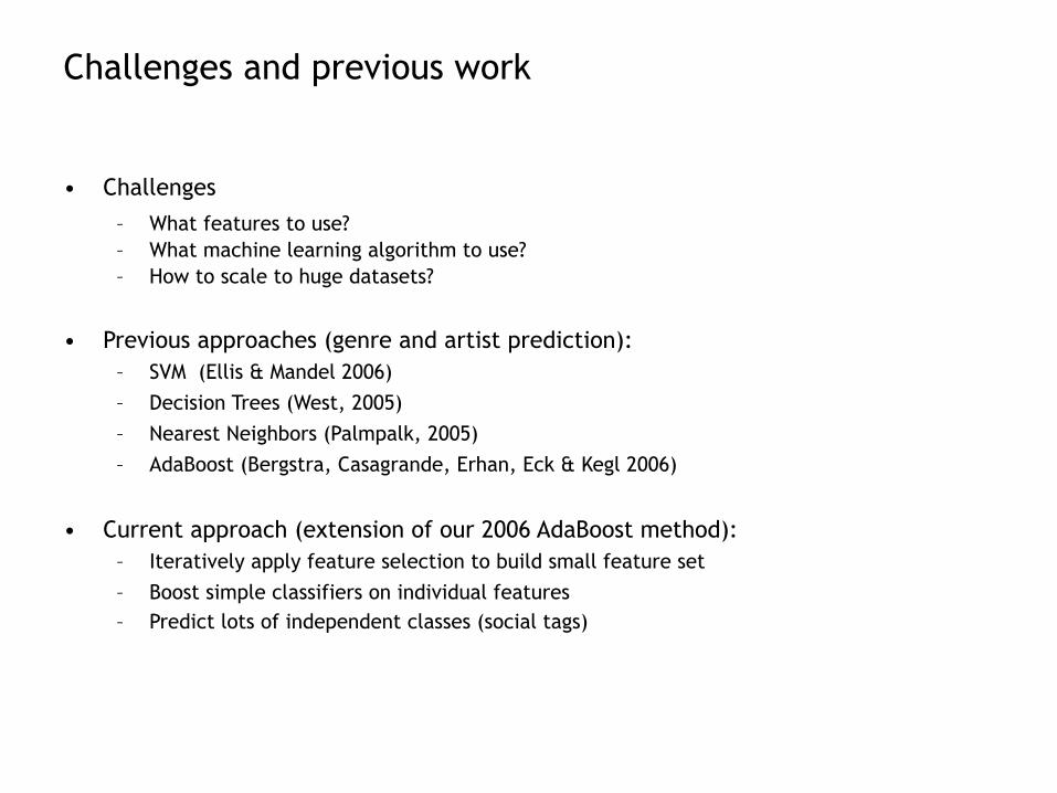
• Challenges– What features to use? – What machine learning algorithm to use?– How to scale to huge datasets?
• Previous approaches (genre and artist prediction):– SVM (Ellis & Mandel 2006)– Decision Trees (West, 2005)– Nearest Neighbors (Palmpalk, 2005)– AdaBoost (Bergstra, Casagrande, Erhan, Eck & Kegl 2006)
• Current approach (extension of our 2006 AdaBoost method):– Iteratively apply feature selection to build small feature set – Boost simple classifiers on individual features – Predict lots of independent classes (social tags)
Feature Extraction
• Extract features from audio which reveal musical content
• Many features come from speech recognition
• Three major categories:
– Spectral features (Fourier Transform; time-->frequency)
Example: Spectrogram
– Cepstral features (Fourier transform of spectral features; time-->frequency-->time)
Classic rock1 INXS 11 Meat Loaf 21 The Rolling Stones 31 Violent Femmes2 Creedence Clearwater Revival 12 Jimmy Buffett 22 The Housemartins 32 The B-52's3 Steppenwolf 13 Tom Petty and the Heartbreakers 23 The Beatles 33 Gin Blossoms4 The Cars 14 ZZ Top 24 Al Green 34 Joe Jackson5 The Psychedelic Furs 15 The Mamas & The Papas 25 Darlene Love 35 The Commitments6 The Zombies 16 The Byrds 26 Fugazi 36 Lloyd Cole and the Commotions7 Eric Burdon and the Animals 17 Tina Turner 27 Bob Dylan 37 Talking Heads8 The Lovin' Spoonful 18 X 28 Arlo Guthrie 38 Cream9 Crowded House 19 Guns N' Roses 29 Elvis Costello 39 Bryan Ferry10 Ramones 20 Elvis Costello & The Attractions 30 Jeff Wayne 40 The Band
1 Sasha & John Digweed 11 The Crystal Method 21 Olive 31 Kraftwerk2 Paul van Dyk 12 Les Rythmes Digitales 22 Laurent Garnier 32 Underworld3 Aqua 13 808 State 23 Eiffel 65 33 John Lydon4 Paul Oakenfold 14 Orbital 24 The Shamen 34 Sneaker Pimps5 Sasha 15 Nortec Collective 25 The Chemical Brothers 35 Electronic6 John Digweed 16 Hybrid 26 Basement Jaxx 36 Boom Boom Satellites7 BT 17 ATB 27 Chicane 37 Massive Attack vs. Mad Professor8 Juno Reactor 18 Leftfield 28 bis 38 Kid Loco9 Ministry of Sound 19 Tangerine Dream 29 Aaliyah 39 Fatboy Slim10 Fluke 20 Daft Punk 30 Brazilian Girls 40 The Other Two
Electronic
Reggae1 Bunny Wailer 11 D'Angelo 21 Parliament 31 Ursula 10002 Burning Spear 12 Third World 22 Ben Harper 32 Erykah Badu3 The Abyssinians 13 OutKast 23 Johnny Nash 33 Bebel Gilberto4 Dennis Brown 14 Sublime 24 John Lennon & Yoko Ono 34 Los Amigos Invisibles5 Jimmy Cliff 15 Aaliyah 25 Big Audio Dynamite 35 Us36 Fugees 16 Jill Scott 26 Gilberto Gil 36 Mandalay7 Peter Tosh 17 George Clinton 27 The Police 37 _Weird Al_ Yankovic8 Steel Pulse 18 Missy Elliott 28 Joss Stone 38 Prince9 The Melodians 19 Fela Kuti 29 Ernest Ranglin 39 Al Green10 Culture 20 Dispatch 30 Sneaker Pimps 40 Soul Coughing
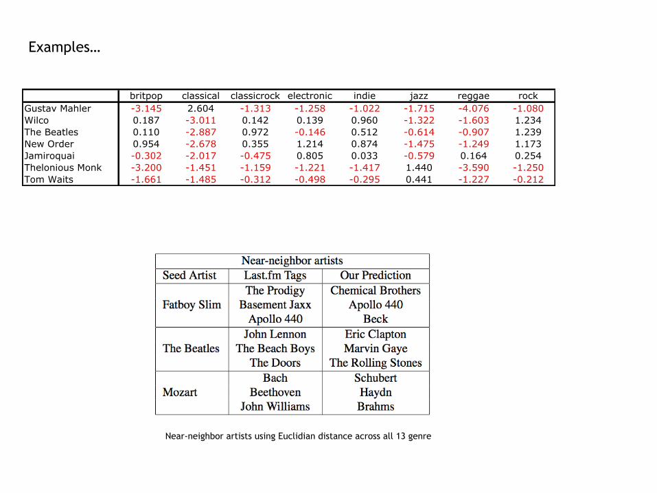
Examples…
Near-neighbor artists using Euclidian distance across all 13 genre
• Currently working on new FilterBoost model with ~2hrs per tag 30
These segment predictions can then be combined to yield artist-level predictions. This can beachieved in two ways: a winning class can be chosen for each segment (in this example the class “alot” would win with 2.6) and the mean over winners can be tallied for all segments belonging to anartist. Alternately we can skip choosing a winner and simply take the mean of the raw outputs for anartist’s segments. Because we wanted to estimate tag frequencies using booster magnitude we usedthe latter strategy.
The next step is to transform these class for our individual social tag boosters into a bag of words tobe associated with an artist. The most naive way to obtain a single value for rock is to look solelyat the prediction for the “a lot” class. However this discards valuable information such as when abooster votes strongly “none”. A better way to obtain a measure for rock-ness is to take the centerof mass of the three values. However, because the values are not scaled well with respect to oneanother, we ended up with poorly scaled results. Another intuitive idea is simply to subtract thevalue of the “none” bin from the value of the “a lot” bin, the reasoning being that “none” is trulythe opposite of “a lot”. In our example, this would yield a rock strength of 7.16. In experimentsfor setting hyperparameters, this was shown to work better than other methods. Thus to generateour final measure of rock-ness, we ignore the middle bin (“some”). However this should not betaken to mean that the middle “some” bin is useless: the booster needed to learn to predict “some”during training thus forcing it to be more selective in predicting “none” and “a lot”. As a large-margin classifier, AdaBoost tries to separate the classes as much as possible, so the magnitude of thevalues for each bin are not easily comparable. To remedy this, we normalize by taking the minimumand maximum prediction for each booster, which seems to work for finding similar artists. Thisnormalization would not be necessary if we had good tagging data for all artists and could performregression on the frequency of tag occurrence across artists.
4 Experiments
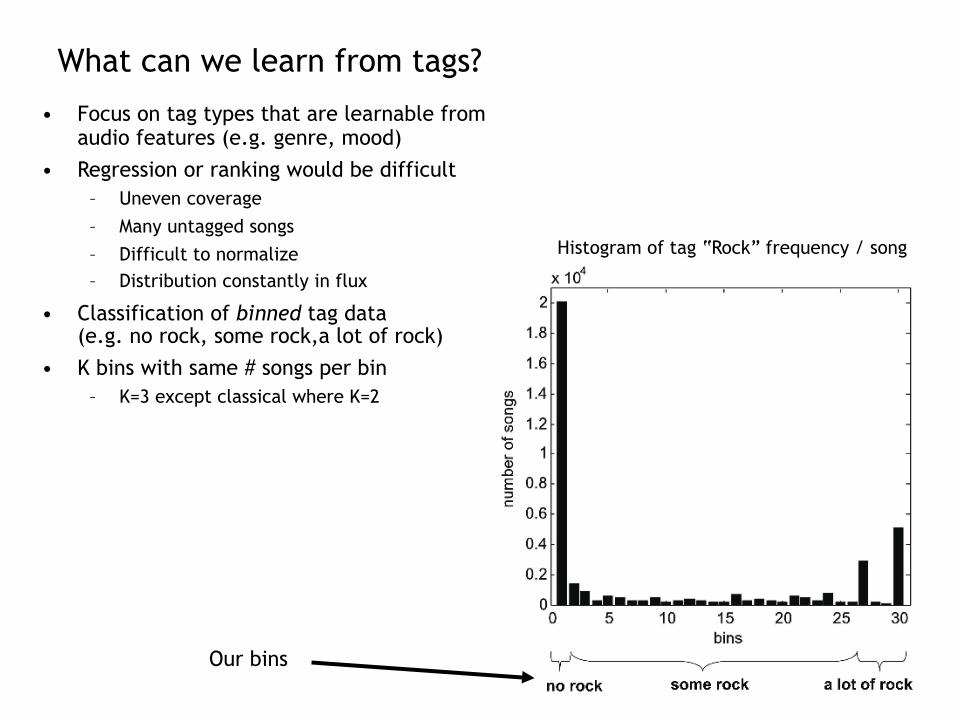
To test our model we selected the 60 most popular tags from the Last.fm crawl data described inSection 2. These tags included genres such as “Rock”, “Electronica”, and “Post Punk”, mood-related terms such as “Chillout”. The full list of tags and frequencies are available in the “extramaterials”. We collected MP3s for a subset of the artists obtained in our Audioscrobbler crawl.From those MP3s we extracted several popular acoustic features. In total our training and testingdata included 89924 songs for 1277 artists and yielded more than 1 million 5s aggregate features.
4.1 Booster Errors
As described above, a classifier was trained to map audio features onto aggregate feature segmentsfor each of the 60 tags. A third of the data was withheld for testing. Because each of the 60boosters needed roughly 1 day to process, we did not perform cross-validation. However eachbooster was trained on a large amount of data relative to the number of decision stumps learned,making overfitting a remote possibility. Classification errors are shown in Table 2. These errors arebroken down by tag in the annex for this paper. Using 3 bins and balanced classes, the random erroris about 67%.
Mean Median Min MaxSegment 40.93 43.1 21.3 49.6Song 37.61 39.69 17.8 46.6
Table 2: Summary of test error (%) on predicting bins for songs and segments.
4.2 Evaluation measures
We use three measures to evaluate the performance of the model. The first TopN compares tworanked lists, a target “ground truth” list A and our predicted list B. This measure is introduced in[2], and is intended to place emphasis on how well our list predicts the top few items of the targetlist. Let kj be the position in list B of the jth element from list A. !r = 0.51/3, and !c = 0.52/3,
5
Similarity Measures• How to measure fit to some known list of similar
artists?
• TopN measures how well we fit the top N artists. Let kj be the position in list B of the jth element from list A.
• TopBucket is percentage of commen elements in top N positions of two ranked lists
31
as in [2]. The result is a value between 0 (dissimilar) and 1 (identical top N ),
si =!N
j=1 !jr!
kjc
!Nl=1(!r ! !c)l
(2)
For the results produced below, we look at the top N = 10 elements in the lists.
Our second measure is Kendall’s Tau, a classic measure in collaborative filtering which measuresthe number of discordant pairs in 2 lists. Let RA(i) be the rank of the element i in list A, if i is notexplicitly present, RA(i) = length(A) + 1. Let C be the number of concordant pairs of elements(i, j), e.g. RA(i) > RA(j) and RB(i) < RB(j). In a similar way, D is the number of discordantpairs. We use " ’s approximation in [8]. We also define TA and TB the number of ties in list A andB. In our case, it’s the number of pairs of artists that are in A but not in B, because they end uphaving the same position RB = length(B) + 1, and reciprocally. Kendall’s tau value is defined as:
" =C "D
sqrt((C + D + TA)(C + D + TB))(3)
Unless otherwise noted, we analyzed the top 50 predicted values for the target and predicted lists.Finally, we compute what we call the TopBucket, which is simply the percentage of common ele-ments in the top N of 2 ranked lists. Here as in Kendall we compare the top 50 predicted valuesunless otherwise noted.
4.3 Constructing ground truth
As has long been acknowledged [4] one of the biggest challenges in addressing this task is to find areasonable “ground truth” against which to compare our results. We seek a similarity matrix amongartists which is not overly biased by current popularity, and which is not built directly from thesocial tags we are using for learning targets. Furthermore we want to derive our measure usingdata that is freely available data on the web, thus ruling out commercial services such as AllMusic(www.allmusic.com). Our solution is to construct our ground truth similarity matrix using correla-tions from the listening habits of Last.fm users. If a significant number of users listen to artists Aand B (regardless of the tags they may assign to that artist) we consider those two artists similar.
One challenge, of course, is that some users listen to more music than others and that some artistsare more popular than others. Text search engines must deal with a similar problem: they wantto ensure that frequently used words (e.g., system) do not outweigh infrequently used words (e.g.,prestidigitation) and that long documents do not always outweigh short documents. Search enginesassign a weight to each word in a document. The weight is meant to represent how important thatword is for that document. Although many such weighting schemes have been described (see [11]for a comprehensive review), the most popular is the term frequency-inverse document frequency(or TF#IDF) weighting scheme. TF#IDF assigns high weights to words that occur frequently in agiven document and infrequently in the rest of the collection. The fundamental idea is that wordsthat are assigned high weights for a given document are good discriminators for that document fromthe rest of the collection. Typically, the weights associated with a document are treated as a vectorthat has its length normalized to one.
In the case of LastFM, we can consider an artist to be a “document”, where the “words” of thedocument are the users that have listened to that artist. The TF#IDF weight for a given user for agiven artist takes into account the global popularity of a given artist and ensures that users who havelistened to more artists do not automatically dominate users who have listened to fewer artists. Theresulting similarity measure seems to us to do a reasonable enough job of capturing artist similarity.Furthermore it does not seem to be overly biased towards popular bands. See “extra material” forsome examples.
4.4 Similarity Results
One intuitive way to compare autotags and social tags is to look at how well the autotags reproducethe rank order of the social tags. We used the measures in Section 4.2 to measure this on 100 artistsnot used for training (Table 3). The results were well above random. For example, the top 5 autotagswere in agreement with the top 5 social tags 61% of the time.
6
These segment predictions can then be combined to yield artist-level predictions. This can beachieved in two ways: a winning class can be chosen for each segment (in this example the class “alot” would win with 2.6) and the mean over winners can be tallied for all segments belonging to anartist. Alternately we can skip choosing a winner and simply take the mean of the raw outputs for anartist’s segments. Because we wanted to estimate tag frequencies using booster magnitude we usedthe latter strategy.
The next step is to transform these class for our individual social tag boosters into a bag of words tobe associated with an artist. The most naive way to obtain a single value for rock is to look solelyat the prediction for the “a lot” class. However this discards valuable information such as when abooster votes strongly “none”. A better way to obtain a measure for rock-ness is to take the centerof mass of the three values. However, because the values are not scaled well with respect to oneanother, we ended up with poorly scaled results. Another intuitive idea is simply to subtract thevalue of the “none” bin from the value of the “a lot” bin, the reasoning being that “none” is trulythe opposite of “a lot”. In our example, this would yield a rock strength of 7.16. In experimentsfor setting hyperparameters, this was shown to work better than other methods. Thus to generateour final measure of rock-ness, we ignore the middle bin (“some”). However this should not betaken to mean that the middle “some” bin is useless: the booster needed to learn to predict “some”during training thus forcing it to be more selective in predicting “none” and “a lot”. As a large-margin classifier, AdaBoost tries to separate the classes as much as possible, so the magnitude of thevalues for each bin are not easily comparable. To remedy this, we normalize by taking the minimumand maximum prediction for each booster, which seems to work for finding similar artists. Thisnormalization would not be necessary if we had good tagging data for all artists and could performregression on the frequency of tag occurrence across artists.
4 Experiments
To test our model we selected the 60 most popular tags from the Last.fm crawl data described inSection 2. These tags included genres such as “Rock”, “Electronica”, and “Post Punk”, mood-related terms such as “Chillout”. The full list of tags and frequencies are available in the “extramaterials”. We collected MP3s for a subset of the artists obtained in our Audioscrobbler crawl.From those MP3s we extracted several popular acoustic features. In total our training and testingdata included 89924 songs for 1277 artists and yielded more than 1 million 5s aggregate features.
4.1 Booster Errors
As described above, a classifier was trained to map audio features onto aggregate feature segmentsfor each of the 60 tags. A third of the data was withheld for testing. Because each of the 60boosters needed roughly 1 day to process, we did not perform cross-validation. However eachbooster was trained on a large amount of data relative to the number of decision stumps learned,making overfitting a remote possibility. Classification errors are shown in Table 2. These errors arebroken down by tag in the annex for this paper. Using 3 bins and balanced classes, the random erroris about 67%.
Mean Median Min MaxSegment 40.93 43.1 21.3 49.6Song 37.61 39.69 17.8 46.6
Table 2: Summary of test error (%) on predicting bins for songs and segments.
4.2 Evaluation measures
We use three measures to evaluate the performance of the model. The first TopN compares tworanked lists, a target “ground truth” list A and our predicted list B. This measure is introduced in[2], and is intended to place emphasis on how well our list predicts the top few items of the targetlist. Let kj be the position in list B of the jth element from list A. !r = 0.51/3, and !c = 0.52/3,
5
where
Similarity Measures continued
32
as in [2]. The result is a value between 0 (dissimilar) and 1 (identical top N ),
si =!N
j=1 !jr!
kjc
!Nl=1(!r ! !c)l
(2)
For the results produced below, we look at the top N = 10 elements in the lists.
Our second measure is Kendall’s Tau, a classic measure in collaborative filtering which measuresthe number of discordant pairs in 2 lists. Let RA(i) be the rank of the element i in list A, if i is notexplicitly present, RA(i) = length(A) + 1. Let C be the number of concordant pairs of elements(i, j), e.g. RA(i) > RA(j) and RB(i) < RB(j). In a similar way, D is the number of discordantpairs. We use " ’s approximation in [8]. We also define TA and TB the number of ties in list A andB. In our case, it’s the number of pairs of artists that are in A but not in B, because they end uphaving the same position RB = length(B) + 1, and reciprocally. Kendall’s tau value is defined as:
" =C "D
sqrt((C + D + TA)(C + D + TB))(3)
Unless otherwise noted, we analyzed the top 50 predicted values for the target and predicted lists.Finally, we compute what we call the TopBucket, which is simply the percentage of common ele-ments in the top N of 2 ranked lists. Here as in Kendall we compare the top 50 predicted valuesunless otherwise noted.
4.3 Constructing ground truth
As has long been acknowledged [4] one of the biggest challenges in addressing this task is to find areasonable “ground truth” against which to compare our results. We seek a similarity matrix amongartists which is not overly biased by current popularity, and which is not built directly from thesocial tags we are using for learning targets. Furthermore we want to derive our measure usingdata that is freely available data on the web, thus ruling out commercial services such as AllMusic(www.allmusic.com). Our solution is to construct our ground truth similarity matrix using correla-tions from the listening habits of Last.fm users. If a significant number of users listen to artists Aand B (regardless of the tags they may assign to that artist) we consider those two artists similar.
One challenge, of course, is that some users listen to more music than others and that some artistsare more popular than others. Text search engines must deal with a similar problem: they wantto ensure that frequently used words (e.g., system) do not outweigh infrequently used words (e.g.,prestidigitation) and that long documents do not always outweigh short documents. Search enginesassign a weight to each word in a document. The weight is meant to represent how important thatword is for that document. Although many such weighting schemes have been described (see [11]for a comprehensive review), the most popular is the term frequency-inverse document frequency(or TF#IDF) weighting scheme. TF#IDF assigns high weights to words that occur frequently in agiven document and infrequently in the rest of the collection. The fundamental idea is that wordsthat are assigned high weights for a given document are good discriminators for that document fromthe rest of the collection. Typically, the weights associated with a document are treated as a vectorthat has its length normalized to one.
In the case of LastFM, we can consider an artist to be a “document”, where the “words” of thedocument are the users that have listened to that artist. The TF#IDF weight for a given user for agiven artist takes into account the global popularity of a given artist and ensures that users who havelistened to more artists do not automatically dominate users who have listened to fewer artists. Theresulting similarity measure seems to us to do a reasonable enough job of capturing artist similarity.Furthermore it does not seem to be overly biased towards popular bands. See “extra material” forsome examples.
4.4 Similarity Results
One intuitive way to compare autotags and social tags is to look at how well the autotags reproducethe rank order of the social tags. We used the measures in Section 4.2 to measure this on 100 artistsnot used for training (Table 3). The results were well above random. For example, the top 5 autotagswere in agreement with the top 5 social tags 61% of the time.
6
A third measure is Kendall’s Tau. Here is the text from the NIPS paper:
Ground truth
• Used Last.fm social tags for popular artists as ground truth.
• Correlations from listening habits• If significant number of listeners all listen
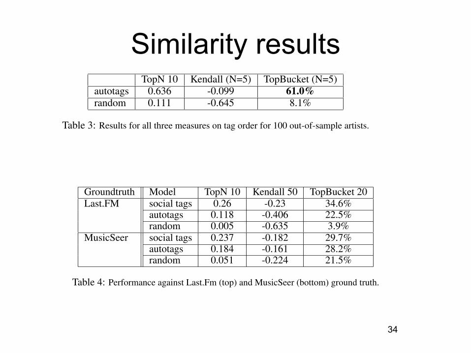
Table 3: Results for all three measures on tag order for 100 out-of-sample artists.
A more realistic way to compare autotags and social tags is via their artist similarity predictions.We construct similarity matrices from our autotag results and from the Last.fm social tags used fortraining and testing. The similarity measure we used wascosine similarity scos(A1, A2) = A1 !A2/(||A1|| ||A2||) where A1 and A2 are tag magnitudes for an artist. In keeping with our interest indeveloping a commercial system, we used all available data for generating the similarity matrices,including data used for training. (The chance of overfitting aside, it would be unwise to remove TheBeatles from your recommender simply because you trained on some of their songs). The similaritymatrix is then used to generate a ranked list of similar artists for each artist in the matrix. These listsare used to compute the measures describe in Section 4.2. Results are found at the top in Table 4.
One potential flaw in this experiment is that the ground truth comes from the same data source asthe training data. Though the ground truth is based on user listening counts and our learning datacomes from aggregate tagging counts, there is still a clear chance of contamination. To investigatethis, we selected the autotags and social tags for 95 of the artists from the USPOP database [2]. Weconstructed a ground truth matrix based on the 2002 MusicSeer web survey eliciting similarity rank-ings between artists from appro 1000 listeners [2]. These results show much closer correspondencebetween our autotag results and the social tags from Last.fm than the previous test. See bottom,Table 4.
Groundtruth Model TopN 10 Kendall 50 TopBucket 20Last.FM social tags 0.26 -0.23 34.6%
Table 4: Performance against Last.Fm (top) and MusicSeer (bottom) ground truth.
It is clear from these previous two experiments that our autotag results do not outperform the socialtags on which they were trained. Thus we asked whether combining the predictions of the autotagswith the social tags would yield better performance than either of them alone. To test this we blendedthe autotag similarity matrix Sa with the social tag matrix Ss using !Sa + (1 " !)Ss. The resultsshown in Figure 3 show a consistent performance increase when blending the two similarity sources.It seems clear from these results that the autotags are of value. Though they do not outperform thesocial tags on which they were trained, they do yield improved performance when combined withsocial tags. At the same time they are driven entirely by audio and so can be applied to new, untaggedmusic. With only 60 tags the model makes some reasonable predictions. When more boosters aretrained, it is safe to assume that the model will perform better.
5 Conclusion and future work
The work presented here is preliminary, but we believe that a supervised learning approach to au-totagging has substantial merit. Our next step is to compare the performance of our boosted modelto other approaches such as SVMs and neural networks. The dataset used for these experimentsis already larger than those used for published results for genre and artist classification. However,a dataset another order of magnitude larger is necessary to approximate even a small commercialdatabase of music. A further next step is comparing the performance of our audio features with othersets of audio features.
7
Similarity results
34
More similarity results
35
Figure 3: Similarity performance results when autotag similarities are blended with social tag simi-larities. The horizontal line is the performance of the social tags against ground truth.
We plan to extend our system to predict many more tags than the current set of 60 tags. We expectthe accuracy of our system to improve as we extend our tag set, especially as we add tags such asClassical and Folk that are associated with whole genres of music. We will also continue exploringways in which the autotag results can drive music visualization. See “extra examples” for somepreliminary work.
Our current method of evaluating our system is biased to favor popular artists. In the future, weplan to extend our evaluation to include comparisons with music similarity derived from humananalysis of music. This type of evaluation should be free of popularity bias. Most importantly, themachine-generated autotags need to be tested in a social recommender. It is only in such a contextthat we can explore whether autotags, when blended with real social tags, will in fact yield improvedrecommendations.
References[1] Audioscrobbler. Web Services described at http://www.audioscrobbler.net/data/webservices/.[2] A. Berenzweig, B. Logan, D. Ellis, and B. Whitman. A large-scale evaluation of acoustic and subjective
music similarity measures. In Proceedings of the 4th International Conference on Music InformationRetrieval (ISMIR 2003), 2003.
[3] J. Bergstra, N. Casagrande, D. Erhan, D. Eck, and B. Kegl. Aggregate features and AdaBoost for musicclassification. Machine Learning, 65(2-3):473–484, 2006.
[4] D. Ellis, B. Whitman, A. Berenzweig, and S. Lawrence. The quest for ground truth in musical artistsimilarity. In Proceedings of the 3th International Conference on Music Information Retrieval (ISMIR2002), 2002.
[5] Y. Freund and R.E. Shapire. Experiments with a new boosting algorithm. In Machine Learning: Pro-ceedings of the Thirteenth International Conference, pages 148–156, 1996.
[6] B. Gold and N. Morgan. Speech and Audio Signal Processing: Processing and Perception of Speech andMusic. Wiley, Berkeley, California., 2000.
[7] Jonathan L. Herlocker, Joseph A. Konstan, and John Riedl. Explaining collaborative filtering recommen-dations. In Computer Supported Cooperative Work, pages 241–250, 2000.
[8] Jonathan L. Herlocker, Joseph A. Konstan, Loren G. Terveen, and John T. Riedl. Evaluating collaborativefiltering recommender systems. ACM Trans. Inf. Syst., 22(1):5–53, 2004.
[9] R. E. Schapire and Y. Singer. Improved boosting algorithms using confidence-rated predictions. MachineLearning, 37(3):297–336, 1999.
[10] Brian Whitman and Ryan M. Rifkin. Musical query-by-description as a multiclass learning problem. InIEEE Workshop on Multimedia Signal Processing, pages 153–156. IEEE Signal Processing Society, 2002.
[11] Justin Zobel and Alistair Moffat. Exploring the similarity space. SIGIR Forum, 32(1):18–34, 1998.
8
Low dimensional music space
• Create low-dimensional space from autotags
• Find shortest path using Isomap
36
37
38
39
Compare two “classical” to “heavy”
40
Beethoven to The Prodigy Mozart to Nirvana
Conclusions
• A simple framework for machine music listening:– Audio feature extraction + segmentation– Ensemble learning (boosting)– Classification of social tags using binning strategy
• Can be improved in many ways:– Ranking or regression– Regularization via weight sharing among song segments– Features derived from human audition– Many, many more features (source identification e.g. is there a female voice?)
• With relatively-simple machine learning, one can:– “Listen to” audio files to know their *musical* content– Embed songs and artists in a rich music space
• Important for companies like Last.FM and Pandora (music recommenders)
• Crucial for any company wanting to know what is going on with music on the web
Bibliography
• D. Eck, P. Lamere, T. Bertin-Mahieux, and S. Green. Automatic generation of social tags for music recommendation. In Neural Information Processing Systems Conference (NIPS) 20, 2007.
• D. Eck, T. Bertin-Mahieux, and P. Lamere. Autotagging music using supervised learning. In Proceedings of the 8th International Conference on Music Information Retrieval (ISMIR 2007), 2007. Submitted.
• J. Bergstra, N. Casagrande, D. Erhan, D. Eck, and B. Kégl. Aggregate features and AdaBoost for music classification. Machine Learning, 65(2-3):473-484, 2006.
• Bergstra, A. Lacoste, and D. Eck. Predicting genre labels for artists using freedb. In Proceedings of the 7th International Conference on Music Information Retrieval (ISMIR 2006), 2006.