MS C AI I NDIVIDUAL P ROJECT I MPERIAL C OLLEGE L ONDON D EPARTMENT OF C OMPUTING Automation and Intelligent Control in High Performance Sailing Boats Final Report Submitted in partial fulfilment of the requirements for the MSc Degree in Artificial Intelligence of Imperial College London Author: Charles Metz (CID: 01825073) Supervisor: Dr Pedro Baiz Second Supervisor: Dr Eric Topham Second Marker: Prof Julie McCann Date: September 4, 2020
Transcript
MSC AI INDIVIDUAL PROJECT
IMPERIAL COLLEGE LONDON
DEPARTMENT OF COMPUTING
Automation and Intelligent Control inHigh Performance Sailing Boats
Final Report
Submitted in partial fulfilment of the requirements for the MScDegree in Artificial Intelligence of Imperial College London
Author:Charles Metz (CID: 01825073)
Supervisor:Dr Pedro Baiz
Second Supervisor:Dr Eric TophamSecond Marker:
Prof Julie McCann
Date: September 4, 2020
Abstract
This study is a continuation of the work of Birk Ulstad, Roman Kastusik and Stanis-las Hannebelle on the application of machine learning methods to the intelligentsteering of sailing boats. The purpose of the study is to investigate models that reli-ably reproduce the behaviour of a sailing boat in its sea environment. These digitaltwins of the sailboat consist of timeseries forecasting models that predict the valuesof various variables that define the state of the boat for the following second. Thisallows a virtual simulation of how the angle of the boat’s rudder affects the boat’scourse and its state, which is the basis for Reinforcement Learning algorithms tolearn intelligent control of the rudder. Detailed background research provides anoverview of relevant developments in the field of timeseries forecasting. The modelsinvestigated here are LSTM-based deep neural networks as well as models derivedfrom first principles. The improvement of the architecture and hyperparameters ofthe models using Bayesian optimisation is discussed. A significant improvement ofthe models compared to a previous approach is achieved. While adequate modelhyperparameters can be found for a given dataset of a given boat, it is found thatthey are not easily generalisable across different data collecting protocols. Finally, aframework with which to obtain and assess accurate forecasting models is proposed.
Keywords: Sailing, Autopilot, Digital Twin, Deep Learning, Recurrent Neural Net-works, LSTM, Bayesian Optimisation, Timeseries Forecasting
1
Acknowledgements
I would like to thank Roman Kastusik and Dr Eric Topham, who during almost fivemonths took time for daily online meetings. Despite otherwise very full agendas,they were always available for enquiries and made me benefit very much from theirexperience, ideas and constructive criticism. I am particularly grateful that they didso during an era marked by a crown-shaped predator, on top of which they allowedme to gain insight into what was happening at their company T-DAB. I would alsolike to thank Dr Pedro Baiz, who contributed his input and knowledge to the projecton a weekly basis; his feedback proved valuable in many ways. I would also liketo thank Stanislas Hannebelle: he took the time to explain various aspects of theproject to me. Finally, I would like to thank Prof Julie McCann, who took the timeto review this and another report and to answer several questions. All in all, I amextremely grateful that this project could take place despite the circumstances.
Modern racing sailboats are masterpieces of engineering: from materials science tocommunication technology and aerodynamics, they combine state-of-the-art tech-nology and science. One area seems to be somewhat excluded from this rapid devel-opment, namely that of sailing autopilots. During races they are estimated to takeover 95% of the steering, but do so with about 80% of the performance of a humanskipper. Hence, there is a large potential to reduce this discrepancy between manand machine by using novel machine learning (ML) methods. Reinforcement Learn-ing (RL) is particularly interesting for this purpose, as it can theoretically result inalgorithms that outperform human behaviour. However, it can only deliver satisfac-tory results if a satisfactory RL simulation environment is available to train it. Sucha training environment corresponds to a time series forecasting model that is ableto predict the next values of the measures that define the state of the sailboat andof its environment. Indeed, the accurate prediction of the latter variables allows toprovide feedback to the RL algorithm about the consequences of its actions.The present project is concerned with the optimisation of this RL simulation environ-ment, i.e. with the elaboration of accurate time series forecasting models. This studyis the fourth in a series of works dealing with ML solutions for sailing autopilots. Anumber of entities are involved in this ongoing project.
1.2 Entities involved in the project
In the following, the entities involved in the present work are presented.
• T-DAB is a London-based company specialising in data science and data en-gineering, offering solutions in a wide range of areas. It was established in2017 and co-founded by Dr Eric Topham. Since 2019, the company has regu-larly offered students the opportunity to complete their master’s theses withinthe company. Roman Kastusik, Birk Ulstad and Stanislas Hannebelle, who areregularly mentioned in the following, took advantage of this opportunity fromJanuary to June and April to September 2019, respectively. They were students
6
CHAPTER 1. INTRODUCTION 1.3. OUTLINE
at Imperial College London at the time and have contributed much of the workon this project to date.
• WisConT is a UK-Chinese joint venture specializing in data science consult-ing that works in collaboration with universities like Imperial College London.It was co-founded by Dr Pedro Baiz, the firm’s CTO, who enables final-yearstudents to conduct their master thesis as part of the JTR AI project.
• Jack Trigger Racing (JTR) is the company of professional skipper Jack Trigger.He regularly takes part in sailing races, such as the Route du Rhum in 2018.A long-term goal is to participate in the Vendee Globe, a single-handed racearound the world, which is considered one of the most prestigious sailing racesin the world. He regularly supplies T-DAB with new data, hence many of thedatasets used in the following are based on him.
• nke Marine Electronics develops high-end instruments and technologies forsailing navigation, including autopilots. The French company is a provider ofnavigation equipment to many professional skippers, including Jack Trigger.Amongst other things, the cooperation with nke allows to address the techni-calities of the on-board data collection and processing.
From here on, the collaboration between the four entities will be referred to as the”JTR AI” project.
1.3 Outline
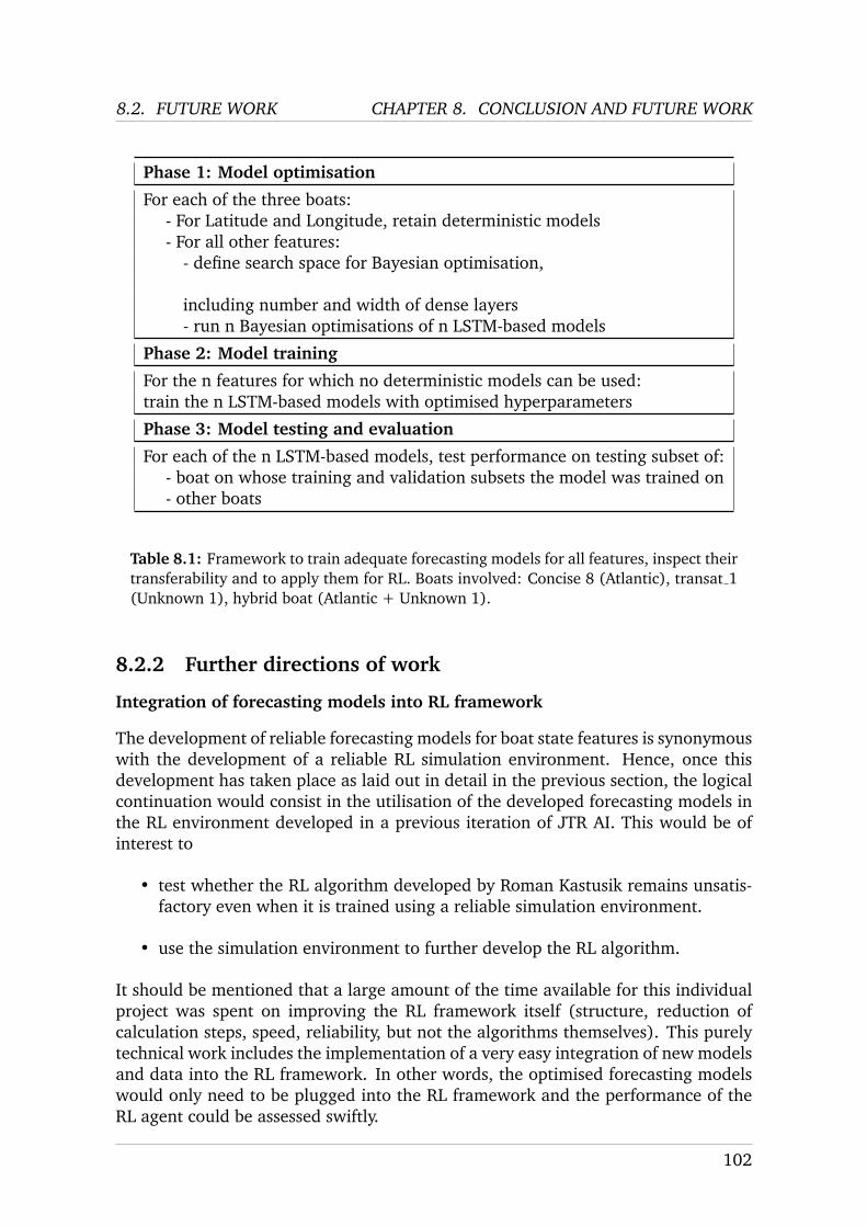
The remainder of this thesis is structured into the following parts:Chapter 2: Background provides an overview of previous works on this project, aswell as of the datasets available for those projects and the current one.Chapter 3: Literature Review presents a systematic literature review of past andcurrent developments in the fields which this thesis relates to, i.e. most notably thatof the development of algorithms for autonomous sailing and of timeseries forecast-ing models. It ends with a presentation of the hypotheses that the present studyaims to verify.Chapter 4: Data presents the preprocessing steps applied to the available datasetsand describes the characteristics of the resulting data, i.e. their statistical distribu-tion and its implication for the present study.Chapter 5: Models introduces the architectures of the deep learning models as wellas the first-principle models that are investigated during the experimentations.Chapter 6: Experiments presents the experimental approach pursued in this study.This includes namely the models trained, the datasets used for training, as well asthe strategy and the metrics employed for assessing the performance of the models.Chapter 7: Results and Evaluation discusses the performance of the models, bothin absolute terms with respect to specific evaluation metrics, as well as in compari-son to the performance of other models.Chapter 8: Conclusion and Future Work presents the conclusions derived from the
7
1.3. OUTLINE CHAPTER 1. INTRODUCTION
presented findings. Furthermore, precise directions of further work are presented, inparticular with respect to the integration of the elaborated simulation environmentinto existing RL algorithms.Chapter 9: Ethical considerations discusses the ethical aspects of the present studyand any work building upon it. In particular, issues relating to data privacy areconsidered. Furthermore, safety concerns in relation to the live deployment of MLalgorithms on sailboats are presented.
8
Chapter 2
Background
The present study forms part of a series of works on JTR AI. Hence, in the following,an overview of the key points of previous works is provided in section 2.1. Further-more, a first overview of the datasets available for JTR AI is presented in section2.2. Finally, in sections 2.3 and 2.4, selected parts of previous works are presentedin deeper detail where they are relevant for the present study.
2.1 Overview of previous work
As mentioned previously, Roman Kastusik, Birk Ulstad and Stanislas Hannebelle havepreviously worked on JTR AI. Their master theses lay the foundations of the projectto date. The work of Roman Kastusik and Birk Ulstad provided in particular the basisfor the parsing and exploitation of data logged during sailing races. This especiallyconcerns the processing of different navigation logs from a format that is specific tothe nke autopilots into a format that is compatible with the application of data anal-ysis and ML methods. Furthermore, both students had the goal to train an ML-basedsailboat autopilot using this data. This ML-based autopilot would steer the boat ina more intelligent manner than conventional autopilots that rely on classical controlschemes. Training ML-based algorithms to ”steer the boat in a more intelligent man-ner” effectively means training these algorithms to compute a position of the rudderthat would be similar to or better than the rudder angle a human sailor would set.Indeed, such a steering behaviour is preferable over the more ”rough” behaviourof traditional closed loop PID controllers that do not directly take into account in-formation about wind, waves and other factors influencing the boat’s course andbehaviour, which leads to their reduced performance. Two fundamentally differentapproaches can be employed to achieve that goal. They have been explored by BirkUlstad, Stanislas Hannebelle and Roman Kastusik and are presented in the following.
2.1.1 Supervised learning approach
Birk Ulstad investigated a supervised learning approach: a model based on recur-rent neural networks (RNNs) and long short-term memory (LSTM) networks was to
9
2.1. OVERVIEW OF PREVIOUS WORK CHAPTER 2. BACKGROUND
learn the behaviour of the skipper (i.e. that of Jack Trigger) using data that had beenlogged during a number of boat races. The model was trained to receive inputs fromenvironmental sensors indicating the physical state of the boat and the environmentaround it, based on which it had to return the same rudder angle as a human skip-per would set in a given situation. Stanislas Hannebelle refined this approach in hismaster thesis, which started a little later, by refining the pre-processing of the data,by training models on different sub-samples of the available data, and by optimizingthe hyperparameters of the models. Compared to the results of Birk Ulstad, this re-sulted in an improvement of the results. Various aspects of this work are relevant tothe present project. They are described in more detail in section 2.3.
2.1.2 RL approach
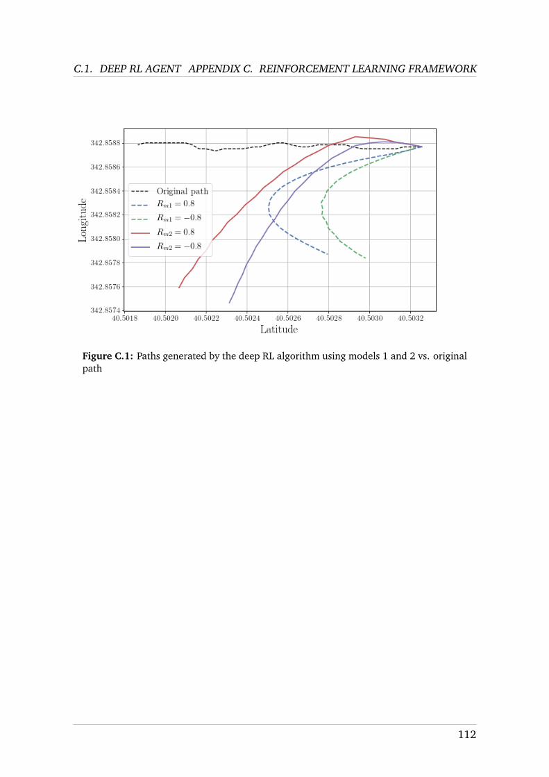
Also described in detail below in section 2.4 is the approach of Roman Kastusik,which was fundamentally different from that of Birk Ulstad and Stanislas Han-nebelle. Instead of a supervised learning approach, where the skipper’s behaviouris only mimicked and can thus at best reach the performance of the data-generatingskipper, Roman Kastusik used deep RL methods. In this approach, the model learnshow to set the rudder to achieve the best possible performance. As explained inmore detail in the appendix C.1, it does so by obtaining rewards or penalties for itsbehaviour. In theory, the model can learn behaviour superior to that of the humanskipper.
Challenges in training a reliable RL simulation environment
However, a deep RL algorithm requires a reliable and as accurate as possible sim-ulation environment of the boat at sea to learn the consequences of its steeringbehaviour and hence be able to learn optimal behaviour. This was a major challengein Roman Kastusik’s master thesis; while the RL agent converged in standard RLtesting environments (further details in appendix C.1), it did not converge in theenvironment developed to simulate the sailboat at sea. This can be attributed to thefact that the amount of data available at that point in time of the JTR AI projectwas not sufficient to train the state estimator (cf. section 2.2). Furthermore, thedatasets available at that point in time present a high degree of bias, as all of themoriginate from races whose routes go from the north-east to the south-west of theAtlantic Ocean. In other words, the state estimator is trained on rather specific sail-ing conditions. Moreover, the relatively small training time of the estimator mighthave been insufficient. Finally and most importantly, the unsatisfactory behaviourcan be attributed to a more sophisticated model architecture and hyperparametersbeing required to capture the dynamics of the boat and its surroundings. Indeed,Roman Kastusik’s study does not include an optimisation of the latter aspect butmerely relied on a single, un-optimised model to provide the simulation environ-ment, which was not fulfilled to a satisfactory degree. Hence, as described in more
10
CHAPTER 2. BACKGROUND 2.2. AVAILABLE DATASETS
detail in section 2.4, improvements to the simulation environment developed by Ro-man Kastusik are possible. Indeed, they constitute the major direction of work of thepresent project, as presented in the sections about the models investigated (5) andabout the experimental strategy pursued in this study (6).Hence, the present study consists in a refinement of the simulation environmentdeveloped by Roman Kastusik. In that light, previous approaches to refining themethods employed by Birk Ulstad and Roman Kastusik are worth considering. Moreprecisely, it is worth taking the optimisations applied to the LSTMs of Birk Ulstad’ssupervised learning approach, and applying those optimisations to the present su-pervised problem for forecasting elements of the boat state more accurately.
2.1.3 Refinement of the existing approaches
It is worth noting that Stanislas Hannebelle’s work consisted largely of a refinementof Birk Ulstad’s works. This is especially true for the data pre-processing and selec-tion of training data, which has been significantly improved by Stanislas Hannebelleand thus contributes to the increase of training data quality, whatever they are usedfor after this step. It also applies to the training of LSTMs in general, especially withrespect to hyperparameter optimization. Stanislas Hannebelle worked this out inthe context of a supervised learning problem for the prediction of an optimal rudderangle. This is different from the present study’s main object of investigation, i.e. theimprovement of boat state estimator. However, the pre-processing step to improvethe data quality and the approach to optimize LSTMs lend themselves for an inte-gration to this study, which is why the relevant parts of Stanislas Hannebelle’s thesisare presented in more detail below in section 2.3.
In this light, the following sections first presents an overview of the available datasets,so that the reader is aware of the data to be used by any models. Subsequently, theparts of Stanislas Hannebelle’s work that are relevant for the present study (datapre-processing, selection of data for model training and hyperparameter optimiza-tion) and the parts of Roman Kastusik’s work important for this study (RL simulationenvironment) are presented. While the understanding of the RL-based approach isnot indispensable for the present study, the interested reader can find an overviewof it in appendix C.1.
2.2 Available datasets
In the following, the different boats for which datasets are available are presented.Subsequently, the datasets used by Roman Kastusik, Stanislas Hannebelle and BirkUlstad are presented. Following this, datasets recently received by T-DAB - and thathave not been used previously in JTR AI - are presented. Finally, tables 2.2 and 2.3provide an overview of the provenance and the format of the datasets. In summary,these datasets essentially consist of key sailing measures (wind speed, boat speedetc.) recorded by different boat sensors during sailing races. A list of the measuresavailable for this thesis is presented in table 2.4 and covered in more detail below.
11
2.2. AVAILABLE DATASETS CHAPTER 2. BACKGROUND
For the sake of consistency, the denominations of the datasets and of features arekept identical as in previous works on JTR AI.
Single-handed and double-handed races It should be stressed that the datasetsdiffer in that they were each generated while either a human skipper or an autopi-lot was in control of the boat. As will be seen in the following, this distinction isparticularly relevant if a model is to be trained to imitate a human skipper usingsupervised learning: in this case, the training requires data generated by a humanskipper. However, as will become apparent subsequently, this distinction is of littlerelevance if a state estimator is to be trained about the physics of the boat, i.e. tolearn its real behaviour on sea independently of a human or an autopilot steeringthe boat. Indeed, in this case it is valuable to benefit from the ensuing increase indiversity of the data, but the data’s being specifically generated by a human skipperor an autopilot is not of relevance.
2.2.1 Types of boats
The different datasets were recorded for different boats - an example of which canbe found in fig. 2.1) - i.e. for
• Jack Trigger’s ”Concise 8”, belonging to the ”Class 40” category of sailingyachts (cf. [1] for further information about this category of sailing yachts).
• Jack Trigger’s ”Virgin Business Media” (VMB), also belonging to the ”Class40” category of sailing yachts.
• two unknown boats that are different from each other but belong to the same”IMOCA 60” category of boats (cf. [2] for the IMOCA 60 rules). In the fol-lowing, both of these boats are denominated ”Unknown 1” and ”Unknown2”.
Table 2.1 presents the technical aspects that define Concise 8, VMB and Unknown1. For Unknown 2, no precise information is available at all and as will be seenin the following sections, it is not necessary for the present study. For VMB, onlyinformation about the sail area is available; for the other technical aspects, the upperlimit is known from the Class 40 rules (cf. [1]). It should be emphasised that inspite of the presented numbers’ corresponding to key characteristics of the boats,these mere numbers do not reflect that e.g. sails of the same sail area might differsubstantially in their cut and hence their behaviour in wind. Another example isweight: it might be exactly identical by the absolute number for two boats, but bedifferently distributed in those two boats. Furthermore, it should be noted that theIMOCA 60-category Unknown 1 differs strongly from the Class 40-category Concise8 and VMB concerning the size, weight and the sail area. This is in line with itsbelonging to the IMOCA 60 class, which essentially is a class of larger and biggerboats than the Class 40. However, while there are differences between the designof Concise 8, VMB and Unknown 1 and therefore their physical behaviour when
12
CHAPTER 2. BACKGROUND 2.2. AVAILABLE DATASETS
sailed, it should be emphasized that all of them have been designed for the sametype of offshore sailing along the same offshore and ocean routes, i.e. for the sameconditions. Thus, notwithstanding the fundamental differences between the boats’dimensions and their behaviour when sailed, they present general similarities intheir design; one could compare them to distant cousins from the same family. Inthis light, it is worth considering the different datasets available for the boats studiedin the present work and the sailing conditions that they contain.
Technical aspect Measure Concise 8 Virgin Media Business Unknown 1Boat class Class 40 Class 40 IMOCA 60Weight [kg] 4500 ≤ 4500 8200Dimensions [m] Length 12.19 ≤ 12.19 18.28
Sail Area [m2] Upwind 115 115 300Downwind 250 250 560
Table 2.1: Technical description of the three boats Concise 8, Virgin Media Business andUnknown 1. Where no precise information is available, upper limits are listed as foundin the Class 40 design rules [1].
13
2.2. AVAILABLE DATASETS CHAPTER 2. BACKGROUND
Figure 2.1: Example of a sailing yacht, from [3]
2.2.2 Concise 8
Four datasets are available for Concise 8. They differ not only in the sailing con-ditions in which they were recorded, but also in the format that was used for theirlogging.
Route du Rhum (nkz)
The Route du Rhum dataset (previously referred to as ”nkz” dataset) was recorded byJTR during parts of the Route du Rhum (RDR) race 2018 and sailed with the Concise8. The dataset was recorded at 25 Hz sampling frequency using nke instruments andsoftware. This was done in the proprietary format of nke, i.e. in the ”.nkz” format.Roman Kastusik and Birk Ulstad spent a considerable time of their master theses on
14
CHAPTER 2. BACKGROUND 2.2. AVAILABLE DATASETS
the conversion of these data into the .csv format for which multiple data processingtools and libraries exist. This was done using the nke software LogAnalyser. Dueto the use of a flash drive not supported by nke’s products during the time of therecording, this dataset is corrupted and data of the Route du Rhum race is onlypartly available. Further information on the used software, the procedure to convertthe data from the .nkz to the .csv format as well as only parts of the data of this racebeing available can be found in Roman Kastusik’s final report [4]. Finally, as theRDR race is single-handed, the autopilot was active during large parts of the race.
Route du Rhum (adrena)
The Route du Rhum (adrena) dataset (previously referred to as ”adrena” dataset)was recorded by JTR during parts of the RDR race 2018 and sailed with the Concise8, much like the nkz dataset. This dataset was generated by passing data of selectedfeatures at a frequency of 1 Hz to the navigation software Adrena running on thesailor’s laptop. It was directly recorded in the .csv format and only when the au-topilot was active, i.e. it does not contain any data of segments sailed by a humanskipper. Details on the dataset can be found in [4].
DRHEAM (18 log)
The DRHEAM 18 dataset (referred to as ”log” dataset in previous works) was recordedby JTR during the DRHEAM cup 2018, sailed with the Concise 8. It was recorded ina specific format that was used before nke introduced the .nkz format. The datasetin this .log format was transformedd into the .csv format by Roman Kastusik by us-ing a specifically adapted parser. Crucially, it should be noted that records in thisformat are made at an inconsistent frequency. The consequences of this will be fur-ther discussed in section 2.3; further information on this format can be found in[4]. DRHEAM cup is a double-handed race, thus this dataset corresponds to a routemainly sailed by two human skippers, as opposed to the nkz and adrena datasets.Hence, this dataset is of relevance if a model is to be trained as a digital twin of ahuman skipper using supervised learning. As will be seen in the following, this is thereason why Stanislas Hannebelle made use of this dataset.
Atlantic
Also newly available is the Atlantic dataset, corresponding to the navigation logrecorded during a delivery made by Jack Trigger in 2019. The delivery was fromthe port of Grenade to the port of Horta on the Azores Island. The recording wasperformed in the .nkz format at 25 Hz and has been converted entirely to the .csvformat. Since this delivery was sailed solo by Jack Trigger, the autopilot was activeduring large parts of the trajectory.
15
2.2. AVAILABLE DATASETS CHAPTER 2. BACKGROUND
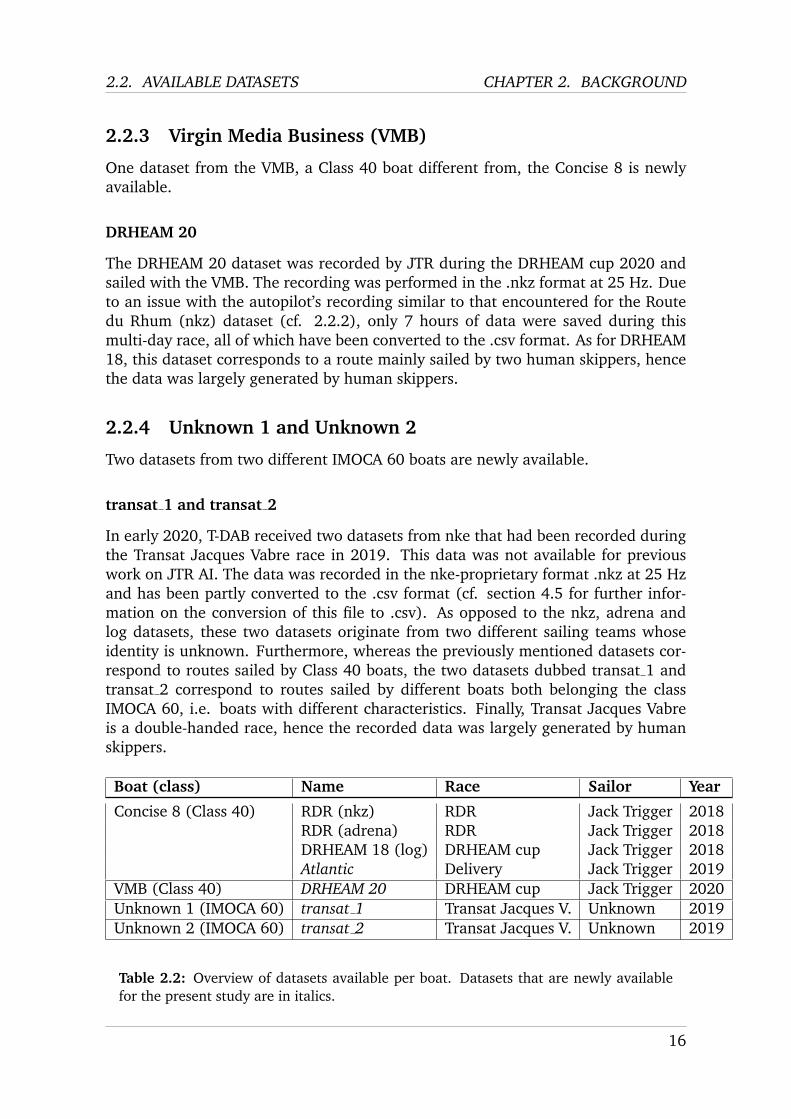
2.2.3 Virgin Media Business (VMB)
One dataset from the VMB, a Class 40 boat different from, the Concise 8 is newlyavailable.
DRHEAM 20
The DRHEAM 20 dataset was recorded by JTR during the DRHEAM cup 2020 andsailed with the VMB. The recording was performed in the .nkz format at 25 Hz. Dueto an issue with the autopilot’s recording similar to that encountered for the Routedu Rhum (nkz) dataset (cf. 2.2.2), only 7 hours of data were saved during thismulti-day race, all of which have been converted to the .csv format. As for DRHEAM18, this dataset corresponds to a route mainly sailed by two human skippers, hencethe data was largely generated by human skippers.
2.2.4 Unknown 1 and Unknown 2
Two datasets from two different IMOCA 60 boats are newly available.
transat 1 and transat 2
In early 2020, T-DAB received two datasets from nke that had been recorded duringthe Transat Jacques Vabre race in 2019. This data was not available for previouswork on JTR AI. The data was recorded in the nke-proprietary format .nkz at 25 Hzand has been partly converted to the .csv format (cf. section 4.5 for further infor-mation on the conversion of this file to .csv). As opposed to the nkz, adrena andlog datasets, these two datasets originate from two different sailing teams whoseidentity is unknown. Furthermore, whereas the previously mentioned datasets cor-respond to routes sailed by Class 40 boats, the two datasets dubbed transat 1 andtransat 2 correspond to routes sailed by different boats both belonging the classIMOCA 60, i.e. boats with different characteristics. Finally, Transat Jacques Vabreis a double-handed race, hence the recorded data was largely generated by humanskippers.
Boat (class) Name Race Sailor Year
Concise 8 (Class 40) RDR (nkz) RDR Jack Trigger 2018RDR (adrena) RDR Jack Trigger 2018DRHEAM 18 (log) DRHEAM cup Jack Trigger 2018Atlantic Delivery Jack Trigger 2019
VMB (Class 40) DRHEAM 20 DRHEAM cup Jack Trigger 2020Unknown 1 (IMOCA 60) transat 1 Transat Jacques V. Unknown 2019Unknown 2 (IMOCA 60) transat 2 Transat Jacques V. Unknown 2019
Table 2.2: Overview of datasets available per boat. Datasets that are newly availablefor the present study are in italics.
16
CHAPTER 2. BACKGROUND 2.3. PREVIOUS WORK BY S. HANNEBELLE
Table 2.3: Overview of the available datasets’ formats and sampling frequencies.Datasets that are newly available for the present study are in italics.
2.3 Previous work by S. Hannebelle
While the present work focuses on improving the simulation environment of thedeep RL algorithm developed by Roman Kastusik, Stanislas Hannebelle’s work [5](building on that of Birk Ulstad [6]) contains many aspects that are useful to thepresent work. The relevant parts of this previous work are presented in more detailin the following sections.
2.3.1 Data Pre-Processing
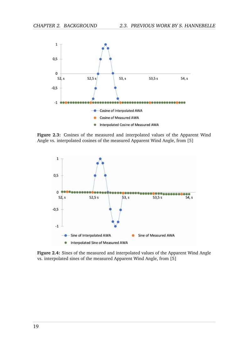
Re-Sampling Data to 25 Hz Stanislas Hannebelle used the DRHEAM 18 (log)dataset, as presented in section 2.2. The measures recorded in this dataset - windspeed, wind angle, position etc. - are presented in detail in table 2.4. In the logdataset, the time differences between the recordings of new states are not consis-tent; they range anywhere between 0.004 and 0.067 seconds. Moreover, many ofthese features come in the form of angles, which entails jumps from -180° to 180°respectively from 180° to -180°, as can be seen in fig. 2.2 (taken from StanislasHannebelle’s master’s thesis [5]). However, for the proper training of the ML mod-els, timeseries data is needed which update at a consistent - and not at a constantlychanging - frequency. For this reason Stanislas Hannebelle further developed a re-sampling algorithm used by Birk Ulstad, which re-samples the data to a constantfrequency of 25 Hz. First, in order to account for the abrupt changes in the angularvalues (e.g. from -180° to 180°), angle values are replaced by their cosine and sinevalues. Subsequently, linear interpolation is used to resample the timeseries inter-vals to a constant 25 Hz. The pseudo code of this approach is shown in algorithm 1.Figures 2.3 and 2.4 serve as an illustration of this first pre-processing step.
17
2.3. PREVIOUS WORK BY S. HANNEBELLE CHAPTER 2. BACKGROUND
Algorithm 1 Re-sampling log data to 25Hz Algorithm
1: procedure TO25HZ(log csv path,log 25Hz csv path)2: log← read csv(log csv path)3: for column ∈ set of angles in range [-180,180] or [0,360] do4: log[column cos]← cos(log[column])5: log[column sin]← sin(log[column])6: log.drop(column)7: end for8: log← log.resample(’00.04S’).asfreq().interpolate(’linear’)9: for column ∈ set of angles in range [-180,180] or [0,360] do
10: log[column]← sign(log[column sin])arccos(log[column cos])11: log.drop(column cos)12: log.drop(column sin)13: end for14: log.save csv(log 25Hz csv path)15: end procedure
Figure 2.2: Measured and interpolated values of the Apparent Wind Angle, from [5]
18
CHAPTER 2. BACKGROUND 2.3. PREVIOUS WORK BY S. HANNEBELLE
Figure 2.3: Cosines of the measured and interpolated values of the Apparent WindAngle vs. interpolated cosines of the measured Apparent Wind Angle, from [5]
Figure 2.4: Sines of the measured and interpolated values of the Apparent Wind Anglevs. interpolated sines of the measured Apparent Wind Angle, from [5]
19
2.3. PREVIOUS WORK BY S. HANNEBELLE CHAPTER 2. BACKGROUND
Feature Name Description Units SourceDataType
Range
Latitude Global coordinate [°] GPS float [-90, 90]
Longitude Global coordinate [°] GPS float [-180, 180]
TWS True wind speed [kts] Derived float [0, 40.0]
TWD True wind direction (global) [°]Derived(GPS)
float [0, 360]
Current speed Speed of water current [kts]Derived(GPS)
float [0,15.0]
Current directionDirection of water current
(global)[°]
Derived(GPS)
float [0, 360]
Air temp Temperature of the air [°C] Measured float [0, 30.0]
Speed ov surfaceSpeed of the boat over the
water[kts] Measured float [0, 25.0]
Speed ov groundSpeed of the boat over the
ground[kts]
Derived(GPS)
float [0, 25.0]
VMG’Velocity made good’, speed
towards wind direction[kts] Derived float [0, 25.0]
Heading True True heading relative to North [°]Derived(mag)
TWATrue wind angle (local, awaaccounting for boat motion)
[°] Derived float [-180, 180]
Rudder(nkz and log
data-sets only)
Angle of the rudder relative toneutral position
[°] Measured float [-30, 30]
Table 2.4: Overview of data available for project, from [4]
20
CHAPTER 2. BACKGROUND 2.3. PREVIOUS WORK BY S. HANNEBELLE
Removal of Tacks
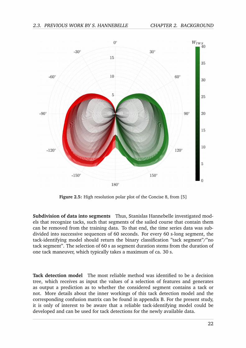
Motivation After their upsampling to a consistent frequency, a second preprocess-ing step is applied to the time series data. Indeed, a sailboat can move in differentdirections relative to the wind. This True Wind Angle between boat and wind deter-mines the performance of the boat to a large extent, especially regarding the boat’sattainable speed for a given True Wind Angle. This is illustrated by fig. 2.5 takenfrom [5], which represents the corresponding polar plot for the Concise 8, the boatsailed by Jack Trigger. In the figure it can be recognized that strong changes are tak-ing place during the process of a tack, i.e. when the True Wind Angle passes 0°, aswell as during the process of a gybe, i.e. when the True Wind Angle passes 180°. Inboth cases the main sail changes the side of the boat. Since the sailed course is sig-nificantly influenced by these tacks and gybes, in the following referred to as ”tacks”for easier reading, the performance of a skipper during a race depends crucially onthem. Moreover, these are quite dangerous maneuvers, as the sails and the boomsweep over the boat and therefore change the balance on board considerably. Thisentails a significant potential for physical damage as well as representing a strongrisk to the skipper. Furthermore, autopilot functions exist for this and are adequate.Moreover, these maneuvers are not critical to performance in offshore sailing, otherthan doing them safely so that the boat remains intact (which if it does not puts anend to the race or even threatens the skipper’s life). Finally, all sorts of reasons canlead to the decision to tack, some relating for instance to strategy or safety, both ofwhich are not available at this time to the autopilot. For these reasons, the modelthat imitates the skipper should not be trained using data containing tacks, but beoptimised with regards to its performance under ”normal” sailing conditions.
21
2.3. PREVIOUS WORK BY S. HANNEBELLE CHAPTER 2. BACKGROUND
Figure 2.5: High resolution polar plot of the Concise 8, from [5]
Subdivision of data into segments Thus, Stanislas Hannebelle investigated mod-els that recognize tacks, such that segments of the sailed course that contain themcan be removed from the training data. To that end, the time series data was sub-divided into successive sequences of 60 seconds. For every 60 s-long segment, thetack-identifying model should return the binary classification ”tack segment”/”notack segment”. The selection of 60 s as segment duration stems from the duration ofone tack maneuver, which typically takes a maximum of ca. 30 s.
Tack detection model The most reliable method was identified to be a decisiontree, which receives as input the values of a selection of features and generatesas output a prediction as to whether the considered segment contains a tack ornot. More details about the inner workings of this tack detection model and thecorresponding confusion matrix can be found in appendix B. For the present study,it is only of interest to be aware that a reliable tack-identifying model could bedeveloped and can be used for tack detections for the newly available data.
22
CHAPTER 2. BACKGROUND 2.3. PREVIOUS WORK BY S. HANNEBELLE
2.3.2 Data Cleaning and Splitting
Two steps of cleaning In a first phase of data cleaning, not only the segmentscontaining a tack were removed, but also the 60-second segment following eachsegment containing a tack. In fact, Jack Trigger had pointed out that it can take upto 60 seconds for the sailboat to return to its speed and optimal sailing conditionsafter a tack, i.e. to return to the conditions that the model should be trained on. In asecond phase of data cleaning, the course of the boat was analysed in detail and seg-ments with anomalies were identified and removed. Indeed, the dataset containedsegments in which abnormal sailing conditions in the form of extremely low windspeeds and low boat speeds appeared. However, since Jack Trigger also stated thatthe model should imitate the boat at full speed and that low wind conditions wereof little relevance. Indeed, while not necessarily appearing as ”outliers” statistically,data of these sections with low wind and/or boat speed does not capture the factthat they entail a very different physical behaviour of the boat. For instance, rockingof the boat can generate apparent wind speed even though there is no wind, simplybecause the mast moves the anemometer through the air as the boat rolls in thewater. With these elements of the boat’s physics being so different, these are not theprimary conditions in which one would expect the autopilot to work. Hence, these”abnormal” segments were removed. This second cleaning step was performed man-ually, i.e. by systematically examining the data for time windows where low windand/or boat speed predominated (cf. [5]) and removing these time windows fromthe data retained for further use. This results in a dataset composed of different timeseries.
Resulting dataset Precisely, for the DRHEAM 18 (log) dataset, the data cleaningleads to 19 different time series. To illustrate, the first time series obtained is ”23rdJuly 2018 from 16:00 to 16:23”, the next one is ”23rd July from 16:25 to 16:36”,etc. For each of these time series, the first 60 % of the segments are concatenatedand retained as training data. The next 20 % of the segments are concatenated torepresent validation data, and the last 20 % are concatenated to represent test data.This allows the model to be trained, validated, and tested on different parts of thedata. This approach takes into account that the conditions are not steady throughoutthe race, nor are they evenly temporally distributed across the race course. By com-posing the training, validation and testing datasets with data from different parts ofthe race, models can be trained and tested on sufficiently similar data. This differsfrom training the model on the first 60 % of the entire time series and validatingand testing it on data from later parts of the sailed route, which would not take intoaccount the uneven distribution of sailing conditions over the race.
2.3.3 Supervised Learning Process
The present study is concerned with the supervised learning problem of trainingreliable models to forecast the multiple variables that describe a boat’s state. Thisproblem has similarities with forecasting the rudder angle a human sailor would set.Hence, it is worth considering the approach taken to solving that problem.
23
2.3. PREVIOUS WORK BY S. HANNEBELLE CHAPTER 2. BACKGROUND
Optimal Sampling Frequency and Input Length
As presented in section 2.3.1, the data is available in a resolution of 25 Hz afterpre-processing. However, the model that is to predict the optimal rudder angle doesnot need to be trained at the maximum frequency of 25 Hz; sampling from the 25Hz dataset by retaining e.g. only every fifth value allows to vary the data granularityof the input provided to the model. A further degree of freedom is the choice ofthe input length of the data, i.e. of the time window of which data is passed to therudder-predicting model. Indeed, as will be elucidated in the literature review, thechoice of the time window for which data is passed to the model heavily influencesthe model’s performance. For these reasons, Stanislas Hannebelle investigated theeffect of different sampling frequencies as well as of different time windows. Indeed,Birk Ulstad in his work used a much more complex model than Stanislas Hannebellefor the same rudder angle prediction task, and obtained the best results for a sam-pling frequency of 5 Hz with a time window of 25 s. However, it was found that thismodel led to severe overfitting (cf. Stanislas Hannebelle’s thesis [5]) that can onlybe compounded when using an even more granular sampling frequency and an evenlonger time window. Stanislas Hannebelle therefore set these two values, 5 Hz and25 s, as upper limits for the sampling frequency and the length of the time window.Furthermore, it was found that the skipper changes the position of the rudder atleast once per second, so 1 Hz was retained as the lower limit for the frequency.In this light, Stanislas Hannebelle trained and validated Birk Ulstad’s model on thepre-processed data as described above for the frequencies {1 Hz, 5 Hz} and for timewindows of the lengths {1s, 2s, 3s, 4s, 5s, 10s, 15s, 20s, 25s}. The retained optimaltime windows were 5 s for a sampling frequency of 1 Hz and 2 s for a sampling fre-quency of 5 Hz. These two combinations were retained as sampling frequency andwindow length for the investigations that followed, and that were namely concernedwith improving the architectures of the supervised learning models. To that end, anoptimisation of the models’ hyperparameters was performed.
Bayesian Optimisation of Hyperparameters
Interest for present study Using the previously mentioned pairs of sampling fre-quency and length of time window, Stanislas Hannebelle trained LSTMs and GRUsto predict the optimal rudder angle. The detail of these networks is of rather littleinterest here (and can be found in the original thesis [5]), since the present workfocuses on predictions of the all of the boat’s features given previous values of theboat’s and the sea’s features, while Stanislas Hannebelle focused on the predictionof the rudder angle only. It is much more the approach to the optimization of thehyperparameters of the models which is interesting for the present study. It is hencedescribed in the following.
Approach The hyperparameters are divided into two classes: First, those whichdefine the architecture of the model and second, those which determine the opti-misation of the model. While Stanislas Hannebelle decided to retain tanh for the
24
CHAPTER 2. BACKGROUND 2.4. PREVIOUS WORK BY R. KASTUSIK
activation functions of the networks and not to experiment with other activationfunctions, he decided to optimise the following measures of the network architec-ture:
• Number of GRU respectively LSTM layers, to control the complexity of themodel
• Number of units per GRU resp. LSTM layer, also to control the complexity ofthe model
• Dropout rate, to influence regularisation
Furthermore, it was decided to use the Adam optimiser because of its proven per-formance in optimisation tasks, and hence not to experiment with different solvers.However, it was decided to optimise the learning rate as it has a significant impacton the speed of the learning process. If these variables were now optimised using agrid search, numerous iterations would have to be run through to identify optimalvalues, which is costly in training time, compute resource, and financial resource.Furthermore, the dropout rate and the learning rate correspond to continuous val-ues in an interval between certain lower and upper limits, which grid search doesnot take advantage of. Bayesian optimisation provides a remedy for both problems,and was therefore retained as an optimisation method. Again, the interested readeris referred to the original thesis for further information on this process [5].
2.4 Previous work by R. Kastusik
Stanislas Hannebelle’s work aimed at refining and improving the pre-processing andhyperparameter optimisation employed by Birk Ulstad, which was a success. Nosuch improvement was conducted for the forecasting model developed by RomanKastusik. However, as outlined in the previous sections, an improvement of thisforecasting model and more broadly of the RL simulation environment is vital forthe progress of an RL-based autopilot. Hence, the following sections present in moreample detail the state estimator developed by Roman Kastusik. Subsequently, thedeep RL model that he developed is presented to the extent relevant for the deepercomprehension of the state estimator’s functioning.
2.4.1 State estimator
The overall data flow developed by Roman Kastusik is presented in figure 2.6, bor-rowed from his final report [4]. A state vector st, describing the estimated state ofthe sea and the boat at instant t, enters a deep deterministic policy gradient (DDPG)RL model. The latter outputs an action at that corresponds to the Rudder Angle atinstant t that the deep RL model predicts to be best at that specific instant t. In thefollowing, these vectors are presented in detail following the exact same denomina-tions as Roman Kastusik used in his report (cf. [4]); this is done in order to ensureconsistency and comparability between the different works on JTR AI.
25
2.4. PREVIOUS WORK BY R. KASTUSIK CHAPTER 2. BACKGROUND
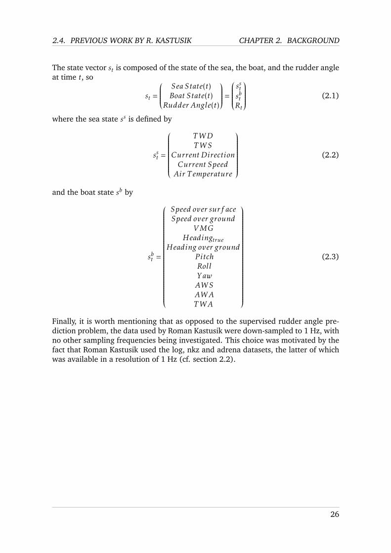
The state vector st is composed of the state of the sea, the boat, and the rudder angleat time t, so
st =
Sea State(t)Boat State(t)
Rudder Angle(t)
=
sstsbtRt
(2.1)
where the sea state ss is defined by
sst =
TWDTWS
Current DirectionCurrent SpeedAir T emperature
(2.2)
and the boat state sb by
sbt =
Speed over surf aceSpeed over ground
VMGHeadingtrue
Heading over groundP itchRollY awAWSAWATWA
(2.3)
Finally, it is worth mentioning that as opposed to the supervised rudder angle pre-diction problem, the data used by Roman Kastusik were down-sampled to 1 Hz, withno other sampling frequencies being investigated. This choice was motivated by thefact that Roman Kastusik used the log, nkz and adrena datasets, the latter of whichwas available in a resolution of 1 Hz (cf. section 2.2).
26
CHAPTER 2. BACKGROUND 2.4. PREVIOUS WORK BY R. KASTUSIK
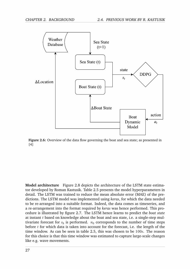
Figure 2.6: Overview of the data flow governing the boat and sea state; as presented in[4]
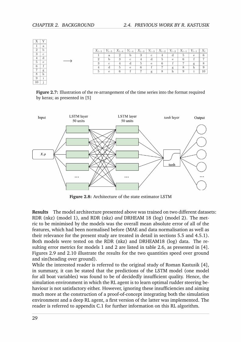
Model architecture Figure 2.8 depicts the architecture of the LSTM state estima-tor developed by Roman Kastusik. Table 2.5 presents the model hyperparameters indetail. The LSTM was trained to reduce the mean absolute error (MAE) of the pre-dictions. The LSTM model was implemented using keras, for which the data neededto be re-arranged into a suitable format. Indeed, the data comes as timeseries, anda re-arrangement into the format required by keras was hence performed. This pro-cedure is illustrated by figure 2.7. The LSTM hence learns to predict the boat stateat instant t based on knowledge about the boat and sea state, i.e. a single-step mul-tivariate forecast for sb is performed. n0 corresponds to the number of time stepsbefore t for which data is taken into account for the forecast, i.e. the length of thetime window. As can be seen in table 2.5, this was chosen to be 100s. The reasonfor this choice is that this time window was estimated to capture large-scale changeslike e.g. wave movements.
27
2.4. PREVIOUS WORK BY R. KASTUSIK CHAPTER 2. BACKGROUND
Metric Value DescriptionN layers 2 Number of LSTM layers in the networkN nodes 50 Number of LSTM units in every layerObserved time n0 [s] 100 Number of time-steps LSTM is fed through
before making predictionDropout 0.35 Proportion of inputs to each of
the layers dropped to avoid overfittingBatch size 60 Number of examples run before gradient is updatedShuffle True Shuffle training examplesStateful False Stateful LSTM
Table 2.5: Model hyperparameters as presented in [4]
28
CHAPTER 2. BACKGROUND 2.4. PREVIOUS WORK BY R. KASTUSIK
Figure 2.7: Illustration of the re-arrangement of the time series into the format requiredby keras; as presented in [5]
Figure 2.8: Architecture of the state estimator LSTM
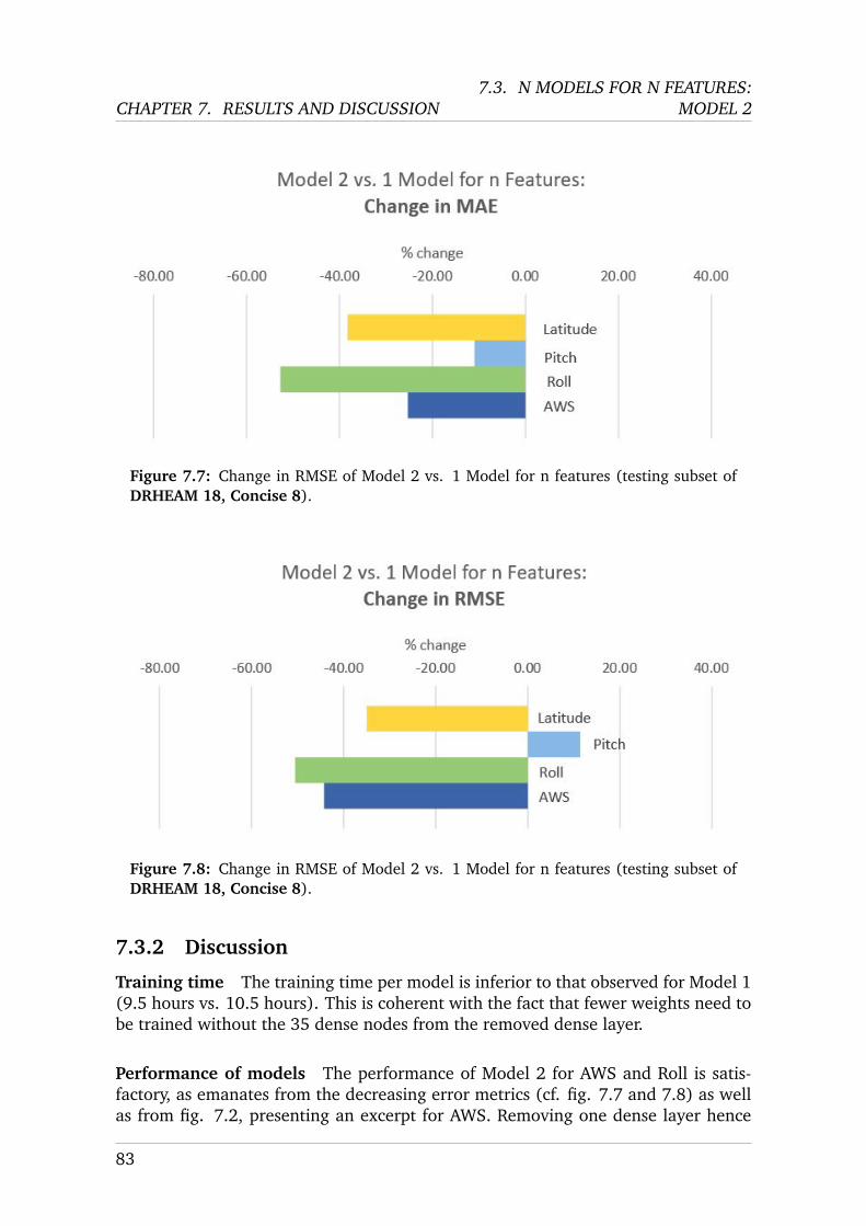
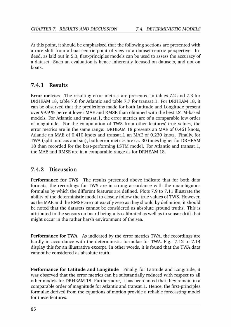
Results The model architecture presented above was trained on two different datasets:RDR (nkz) (model 1), and RDR (nkz) and DRHEAM 18 (log) (model 2). The met-ric to be minimised by the models was the overall mean absolute error of all of thefeatures, which had been normalised before (MAE and data normalisation as well astheir relevance for the present study are treated in detail in sections 5.5 and 4.5.1).Both models were tested on the RDR (nkz) and DRHEAM18 (log) data. The re-sulting error metrics for models 1 and 2 are listed in table 2.6, as presented in [4].Figures 2.9 and 2.10 illustrate the results for the two quantities speed over groundand sin(heading over ground).While the interested reader is referred to the original study of Roman Kastusik [4],in summary, it can be stated that the predictions of the LSTM model (one modelfor all boat variables) was found to be of decidedly insufficient quality. Hence, thesimulation environment in which the RL agent is to learn optimal rudder steering be-haviour is not satisfactory either. However, ignoring these insufficiencies and aimingmuch more at the construction of a proof-of-concept integrating both the simulationenvironment and a deep RL agent, a first version of the latter was implemented. Thereader is referred to appendix C.1 for further information on this RL algorithm.
29
2.4. PREVIOUS WORK BY R. KASTUSIK CHAPTER 2. BACKGROUND
Table 2.6: Error metrics obtained for model 1 and model2; as presented in [4]
Figure 2.9: Prediction of speed over surface (model 2)
30
CHAPTER 2. BACKGROUND 2.4. PREVIOUS WORK BY R. KASTUSIK
Figure 2.10: Prediction of sin(heading over ground) (model 2)
31
Chapter 3
Literature Review
For the reasons mentioned in the previous sections, it should be obvious to thereader that an improvement of the simulation environment would result in signif-icant progress, both in the results for the existing RL algorithm and in a possiblefurther development of that algorithm. This task corresponds essentially to a multi-variate timeseries forecasting problem. The corresponding literature is examinedin more detail in the following. First, for completeness, an overview of researchin the field of autonomous sailboats is provided. Subsequently, an overview of thedevelopment and current state-of-the-art of timeseries forecasting is provided.
3.1 Autonomous sailboats
3.1.1 RoboSail Project
In the early 2000s, a group led by Dr Pieter Adriaans carried out significant pioneer-ing work in the field of autonomous sailing boats. In the so-called RoboSail Project,an attempt was made to transfer then novel AI methods to the control of sailingboats. More detailed information on this can be found in the corresponding publi-cation [7] and on the project website [8]. The project was tested on a real sailingyacht, the ”Syllogic Sailing Lab Open 40”, and in real sea conditions and helped theteam win the ”Round Britain and Ireland” sailing race in 2002. It was also used onthe sailboat ”Kingfisher Open 60”, which made it possible to cross the Atlantic andalso achieved good results for this larger boat.
The AI system owed its success to the development of a hierarchy of tasks on board.A human user can give the system their expert knowledge; under them act four sys-tems which simulate the Skipper, the Navigator, the Watchman and the Helmsman.Each of these systems covers different task areas and time scales, as presented intable 3.1, borrowed from [8].
32
CHAPTER 3. LITERATURE REVIEW 3.1. AUTONOMOUS SAILBOATS
Figure 3.1: Hierarchy used in the RoboSail project, table borrowed from [8]
3.1.2 Other research on autonomous sailboats
To the best of my knowledge, the RoboSail project is the only project with strongsimilarities to the JTR AI project. However, since the RoboSail project, different ad-vances have been realised on aspects of strong relevance for autonomous sailboats.
One of these directions concerns the modelling of waves, which are an importantcomponent of the sailboat’s environment and strongly influence the behaviour ofthe skipper. In fact, a human skipper tries to adjust the rudder angle such that theboat surfs on waves, i.e. such that the speed of the boat is increased by taking ad-vantage of the waves. This also largely explains why human skippers perform betterthan classic autopilots, which essentially stick to a certain direction of the boat andrefrain from making intelligent use of the waves. An intelligent autopilot wouldhence take advantage of the waves; to that end, it would have to have the relevantinformation or modelling at its disposal.
In this context Duz, Mak et al. have investigated the real time estimation of wavecharacteristics [9]. For this purpose, the performance of artificial neural networkswas examined, which are trained to determine the wave height, the wave period andthe wave angle (angle of the wave in relation to the boat) on the basis of a time-series of the 6 degrees of freedom (DOFs) of the boat (pitch, roll, yaw angles andlatitude, longitude as well as vertical position). Further information is not providedto the models; they are ”ship-agnostic”. A multivariate LSTM-CNN and a SlidingPuzzle Network were investigated. Good results were obtained for the modelling ofthe wave angle and of the wave height; for the wave period the results remainedimprovable. It should be noted, however, that the input data included the verticalposition of the boat, a variable that is not available in the data used in this thesis.
Shen, Wang et al. also present a model to describe wave sizes in their work [10].However, the model used is highly simplified and assumes 4 DOFs to describe theboat state (roll and yaw angle, longitude and latitude); an exact description of thewave characteristics is not the primary goal of this work. Rather, it is the optimi-sation of an unmanned sailboat’s speed using a first-principles approach to describethe boat’s dynamics. On the basis of the latter, a feedforward and feedback controlscheme is developed, by which the boat should reach the maximum speed in a givendirection according to the speed polar diagram (cf. figure 2.5).
33
3.2. TIMESERIES FORECASTING:EVOLUTION AND STATE OF THE ART CHAPTER 3. LITERATURE REVIEW
Another approach based on first-principles was presented by Deng, Zhang in [11]. Afirst principles model of a catamaran allowed them to optimize the path following ofthe catamaran, which essentially consists in the catamaran’s following a number ofwaypoints (i.e. coordinates) that together constitute the route to be sailed. This dif-fers from the approach explored by Roman Kastusik described in C.1 towards whichthe present study contributes, which essentially consists in an RL agent learning to beas close as possible or even ahead of a real boat for which data have been gathered,but not in following a route described by waypoints as closely as possible. Further-more, the focus of Deng, Zhang et al.’s work is on optimizing the control systemof the catamaran: a ”robust fuzzy control scheme” is used to optimise the classicalcontrol scheme of the boat, which constitutes the central part of this work. Whilethe work includes practical considerations like the saturation of actuators, the use ofneural networks architectures is not further explored. Finally, Zhang et al. presentin [12] ”a waypoint-based path-following control for an unmanned robot sailboat”.Again, a first-principles model is used and the study focuses on the optimization ofthe control system of the unmanned sailboat. However, within the closed-loop con-trol system, Radial Basic Function Neural Networks (RBF-NNs) are used to optimizethe structure and parameters control scheme. Again, machine learning methods areonly used to improve a classical control loop of an autonomous sailboat, while theiruse for simulating the boat’s environment is not investigated.
3.2 Timeseries Forecasting:Evolution and State of the Art
As mentioned previously, the present work is mainly concerned with accurately fore-casting a boat’s future states in a complex, noisy and dynamic environment. Time-series forecasting is a broad field with many applications: engineering, finance andretail are only some of the areas where timeseries can be used to generate forecast-ing value by predicting system states, stock prices or sales figures. Accordingly, thisfield has long been the object of many research activities.
A good overview of the evolution of state-of-the-art methods in the field of timeseriesforecasting can be found in the work of De Gooijer and Hyndman [13], who presentthe developments in the field from 1980 to 2006 and present multiple different ap-proaches, including ARIMA, exponential smoothing and Kalman filters. Similarly, agood overview of the development of ML methods for timeseries forecasting until2010 can be found in Ahmed, Atiya et al. [14], who describe the development ofmultilayer perceptrons, Bayesian neural networks, k-nearest neighbours and othermethods for timeseries forecasting until 2010. Taieb, Bontempi et al. also reviewdifferent methods for timeseries forecasting until 2012 [15], and study the (improv-ing) effect of deseasonalisation on forecast accuracy.
While the above-mentioned studies primarily depict the development of timeseriesforecasting until about 2010, Parmezan, Souza et al. present a comprehensive
34
CHAPTER 3. LITERATURE REVIEW3.3. DEEP LEARNING FOR
TIMESERIES FORECASTING
overview and evaluation of state-of-the-art models for timeseries forecasting ([16],2019). The publication is particularly interesting for readers who want to get a goodoverview of both statistical methods (e.g. SARIMA) and machine learning algorithms(artificial neural networks, support vector machines, kNNs), and at the same timeget a comprehensive introduction into the timeseries forecasting problem. Finally,Zheng authored a comprehensive report on trajectory data mining [17], providinga useful overview of problems, solutions and metrics applicable to data mining inthe context of trajectory data. Although this study is motivated by and focused ontrajectory data generated by mobile phones, it presents useful methods for trajectoryoutlier detection, trajectory uncertainty and trajectory classification.
3.3 Deep Learning forTimeseries Forecasting
As is apparent from the previous section, novel machine learning methods are in-creasingly present in the field of timeseries forecasting. Deep learning in particularis playing an increasingly prominent and successful role. In the following, recentdevelopments and state-of-the-art deep learning approaches to the timeseries fore-casting problem with particular relevance for the present project will be listed.
Abbasimehr, Shabani et al. present a model based on an LSTM network for de-mand forecasting [18]. While their model is of little relevance to the present project,the comprehensive literature review on timeseries forecasting with a special focus onRNN models is of particular interest. Similarly interesting is the publication by Sezer,Gudelek et al., who present a systematic overview of financial timeseries forecastingusing deep learning techniques [19]. Despite the limitation to financial timeseries,the publication provides useful insights as it discusses MLPs, RNNs, Deep Belief Net-works and deep RL in detail, all of which are methods that are also transferableto forecasting of other types of timeseries. As will be shortly touched upon in sec-tion 2.1, a relevant and much-noticed aspect of timeseries forecasting concerns thelength of the time window which deep learning models are given as input. This isalso of interest for the present paper, since the input time window is crucial for theperformance of the model. In that light, Zhang, Wu et al. investigate the simultane-ous input of four different lengths of a timeseries into an RNN model for an electricload forecasting task [20]. This method allows to capture phenomena that occuron different time scales. The authors of the study explicitly propose to apply themethod in other fields and to test its application to bidirectional LSTMs (BLSTMs).
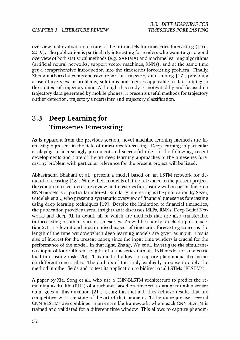
A paper by Xia, Song et al., who use a CNN-BLSTM architecture to predict the re-maining useful life (RUL) of a turbofan based on timeseries data of turbofan sensordata, goes in this direction [21]. Using this method, they achieve results that arecompetitive with the state-of-the-art of that moment. To be more precise, severalCNN-BLSTMs are combined in an ensemble framework, where each CNN-BLSTM istrained and validated for a different time window. This allows to capture phenom-
35
3.3. DEEP LEARNING FORTIMESERIES FORECASTING CHAPTER 3. LITERATURE REVIEW
ena with different time windows and to reflect them in the model. Figures 3.2 and3.3 from the publication of Xia, Song et al. [21] illustrate the method.
The use of different time windows is taken to extremes by Baig, Ibal et al. whouse adaptive time windows instead of static time windows as input to timeseriesforecasting models [22], at least during training. Using this method, they achievestate-of-the-art results for a single-step uni-variate timeseries forecasting problemconsisting in the estimation of resource utilisation of a data center.
Since multi-variate timeseries forecasting is relevant for the present project - theboat state sb presented in 2.4 is a vector containing more than one value - the studyby Du, Li et al. is of interest, which presents a ”novel temporal attention encoder-decoder model” based on BLSTMs [23]. It achieves good results when applied toreal-world timeseries (air quality, power consumption, traffic). Finally, a publicationby Bandara, Bergmeir et al. proposes to use clustered timeseries to train LSTMs ontimeseries forecasting [24]. The clustering allows to construct different models forthe different timeseries clusters and is designed to be applicable to not only LSTMsbut other types of RNNs as well, which is found to augment the forecast accuracy.
Figure 3.2: Framework of the CNN-BLSTM base model proposed by Xia, Song et al.[21]
36
CHAPTER 3. LITERATURE REVIEW3.3. DEEP LEARNING FOR
TIMESERIES FORECASTING
Figure 3.3: CNN-BLSTM training procedures with multiple time windows as proposedby Xia, Song et al. [21]
37
3.4. GENERATIVE ADVERSARIAL NETWORKSFOR TIMESERIES FORECASTING CHAPTER 3. LITERATURE REVIEW
The application of generative adversarial networks (GAN) in the field of timeseriesis a relatively recent development, but offers interesting perspectives. These will bediscussed in the following.
A milestone in this field was set by the paper of Esteban, Hyland et al. in whichGANs are used for the generation of synthetic timeseries data [25]. Using multi-variate medical timeseries data from an intensive care unit station, synthetic multi-variate timeseries are generated. The generated data prove their worth by first train-ing timeseries forecasting models on the synthetic timeseries, and then testing themsuccessfully on the original, real timeseries (”Train on Synthetic, Test on Real” orTSTR). This approach is of particular interest in the medical field, where timeseriesis needed for the training of medical staff, but is not readily available due to strin-gent privacy regulations.
This method has also been applied by Hartmann, Schirrmeister et al. who presentmodified Wasserstein GANs for the generation of synthetic electroencephalogram(EEG) timeseries [26]. In this paper, the GANs are also successfully used for dataaugmentation as well as restoration of corrupted data segments. Using a similarapproach, Fekri, Ghosh et al. use GANs to generate synthetic energy consumptiontimeseries [27].
The use of GANs has thus also been introduced in the area of timeseries, but asdescribed above mainly for the generation of synthetic timeseries. A paper that usesthis approach to make predictions about future system states is that of Li, Chen etal. [28]. It presents a method to detect anomalies using GANs for multivariate time-series. Using a GAN based on an LSTM-RNN architecture, the distribution of themultivariate timeseries of a number of sensors and actuators in a water treatmentsystem under normal conditions is learned. Instead of discarding the discriminatorafter the training of the generator, in the production phase, the discriminator is usedto detect anomalies in the timeseries.
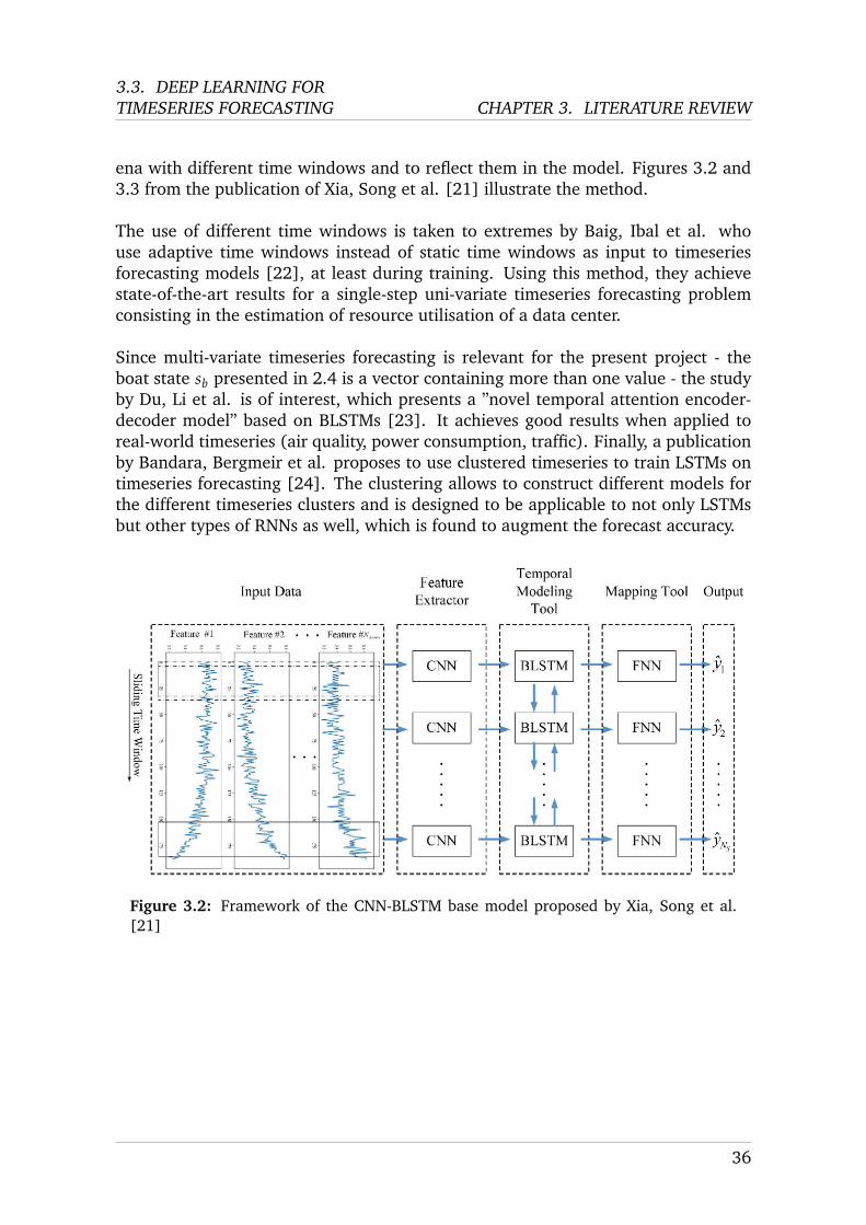
Finally, Koochali, Schichtel et al. present a method to use GANs for single-steptimeseries forecasting [29]. They present good results when applied to timeseries ofnonlinear dynamic systems, especially when the data present strong noise. Figure3.4 presents an overview of the proposed architecture; figure 3.5 presents the de-tails of the generator and the discriminator architectures. From these figures, it canbe seen that the generator learns to generate good ”fake” values for the next pointin time of a given timeseries, and the discriminator learns to recognize these fakes.This trains a generator to make plausible fakes, i.e. good forecasts. Strong results ontwo different nonlinear dynamic systems are found. The authors explicitly suggestapplying the method to multi-step problems as a direction of further work.
38
CHAPTER 3. LITERATURE REVIEW3.4. GENERATIVE ADVERSARIAL NETWORKS
FOR TIMESERIES FORECASTING
Figure 3.4: Overview of the architecture proposed by Koochali, Schichtel et al. [29]
39
3.5. HYBRID MODELS OF DYNAMIC SYSTEMSCHAPTER 3. LITERATURE REVIEW
Figure 3.5: Detailed architectures of the generator (a) and the discriminator (b) asproposed by Koochali, Schichtel et al. [29]
3.5 Hybrid Models of Dynamic Systems
If first-principles models and ML models are presented separately in the previoussections, there is also an approach to combine first-principles methods with ML ap-proaches to reliably forecast the behaviour of real-world dynamic systems. Roughlysummarized, these so-called hybrid models aim to exploit the best of both worldsby making a timeseries forecast based on a first-principles model, which is then im-proved by ML models by the deviations from the values found in the real world.
40
CHAPTER 3. LITERATURE REVIEW3.6. CONCLUSION AND RESULTING
SCOPE OF THE STUDY
Rasheed, San et al. present an overview of the evolution and current state-of-the-art of this approach to dynamic systems modeling in the broader context of ”digitaltwins” of physical systems [30]. Parish and Carlberg present a comprehensive and in-depth coverage of the mathematical details of hybrid models, especially with respectto error modeling [31]. An example for the concrete application of hybrid models isprovided by Wu, Rincon et al., who embed a model based on physical principles intoan RNN network structure to model nonlinear chemical processes [32]. Finally, Mo-hajerin and Waslander apply hybrid models for multi-step prediction of timeseries oftwo dynamic systems, namely a helicopter and a quadrocopter [33]. Furthermore,they present a novel method for an improved initialisation of RNNs.
3.6 Conclusion and resultingscope of the study
As seen in the previous sections, research into intelligent autopilots for sailboats hasbeen very little explored. Although Adriaans et al. pioneered this domain in the early2000s, no comparable comparable work has been conducted since. Even though au-tonomous sailboats have enjoyed further research, especially in the field of control,no comprehensive project like the one by Adriaans et al. has been undertaken since.
3.6.1 Conclusion
Motivation for choices
However, the supervised rudder prediction problem showed that one can achievevery good performance of single step uni-variate forecasting. Roman Kastusik’swork showed that RL could potentially be applied to the rudder prediction prob-lem. Nonetheless, this remains unproven due to the unsatisfactory performanceof the forecasting model. It follows that an improved simulation environment is apromising research area. This corresponds essentially to a single-step multivariatetimeseries forecasting problem. It should be emphasised that the development ofreliable forecasting models for a satisfactory RL simulation environment constitutesone major step in the advancement of the RL-based approach to this problem. How-ever, it does not guarantee that the RL algorithm itself is satisfactory.
Possible directions of investigation
Different directions are possible to solve the single-step multi-variate forecastingproblem and have been researched extensively. Especially the application of DeepLearning in this domain has been an object of strong interest recently. Additionally,novel approaches using GANs for forecasting hold potential. Finally, hybrid modelshave also been explored for this task.
41
3.6. CONCLUSION AND RESULTINGSCOPE OF THE STUDY CHAPTER 3. LITERATURE REVIEW
Choice of direction of investigation
As deep learning and more specifically RNN architectures have recently deliveredpromising results for many and partly comparable cases, it was decided to analysethis approach in a first phase of the study. Moreover, since this field is currently be-ing actively researched, the present study might also result in a contribution to thissubject of interest. The investigation of GANs for forecasting could be of interest forfuture studies. Indeed, the field is currently being actively explored and interestingcontributions could result if its methods were to be applied the problem at hand. Pre-cisely, the applicability of GANs for forecasting could be investigated for the presentproblem, which is of higher complexity than the problems investigated in previousstudies (notably Koochali, Schichtel et al. [29]). However, successful outcomes areless probable with this less explored approach than with the Deep Learning archi-tectures, which have been researched quite extensively. Finally, hybrid models werenot retained for further investigation. The degree of novelty of this field and thus apossible contribution to this research area would be rather insignificant.
3.6.2 Scope of the study
Following the conclusions from above, the overarching goal of the present study wasdefined as the development of a reliable RL simulation environment. This simulationenvironment effectively corresponds to a reliable forecasting model of the boat statefeatures, as developed in a first, but decidedly unsatisfactory attempt by Roman Kas-tusik (cf. section 2.4.1).
Two aspects need to be addressed to that end. On the one hand, a data pipelinemust be established such that the models can be trained, validated and tested onsuitable data. Second, a strategy must be defined to develop the reliable forecastingmodels.
Data pipeline
The pipeline must
1. convert the data from their nke-proprietary format (.nkz) to a format for whichdata analysis and ML libraries are available (.csv).
2. clean the data from any corrupted and irrelevant recordings.
3. allow to consider the distribution and main characteristics of the data.
4. allow to select data that is conducive to the aim of identifying reliable fore-casting models.
5. preprocess the data, i.e. apply any required mathematical transformationsto it, as well as ensure its format corresponds to the format required by theforecasting models.
42
CHAPTER 3. LITERATURE REVIEW3.6. CONCLUSION AND RESULTING
SCOPE OF THE STUDY
In summary, the pipeline must ensure that data is transformed from its raw .nkzstate to a clean state in which it can be used by forecasting models.
Strategy to identify forecasting models
Using this data, the overarching goal of the present study can be pursued, i.e. theidentification of reliable forecasting models. To that end, a progressive approach ischosen, consisting in the successive verification of the following hypotheses:
1. Hypothesis 1: the performance of 1 model for n boat state features, asused by Roman Kastusik, can be improved by optimising the model’s hy-perparameters.On the basis of the satisfying results of the Bayesian optimisation in the rudderprediction problem (section 2.3.3), Bayesian optimisation is employed for thisstep. It aims at clarifying whether the original model can be improved at all,as well as to assess whether the optimised model’s accuracy is satisfactory.
2. Hypothesis 2: training n separate forecasting models for n boat state fea-tures yields more accurate predictions than training 1 model for n fea-tures.The underlying rationale is that a single model for n features must optimise thepredictions for all features at once, i.e. it optimises towards one overall errormetric. In contrast, training n models separately for n features allows eachmodel to be trained only on those dynamics that matter for ”its” predictions.This could potentially result in more accurate forecasting models, which is thefocus of this study.
3. Hypothesis 3: if a model’s hyperparameters lead to inaccurate predic-tions, removing one dense layer improves the prediction accuracy.Indeed, not the same level of complexity may be required to be captured byeach model; architectural changes might be able to take this into account. Pre-cisely, as has been described by Talathi et al. [34], dense layers can directlyinfluence the level of complexity that a model might take into account.
4. Hypothesis 4: Where they can be used, deterministic models achieve bet-ter performance than LSTM-based models.Some boat state features behave according to formulae derived from defini-tions or physical first principles. These formulae might be able to predict valuesbetter than models based on deep learning, as they encapsulate the true phys-ical relations between features. Indeed, the overarching goal of the presentstudy consists in the identification of reliable forecasting models. These do notneed to be deep learning models per se.
5. Hypothesis 5: Where they can be used, deterministic models serve as anindicator of a dataset’s inaccuracies.As mentioned in the previous point, certain features are defined as direct andunambiguous functions of other features. One can hence compute these fea-tures’ values by deterministic models and compare them to the ”true” values
43
3.6. CONCLUSION AND RESULTINGSCOPE OF THE STUDY CHAPTER 3. LITERATURE REVIEW
recorded in the datasets. Any deviations between the two should be an indica-tor of inaccuracies in that dataset.
6. Hypothesis 6: Hyperparameters of forecasting models that are accuratefor a specific data format can be used to train accurate forecasting modelsfor the same boat, but using data of another data format.Indeed, the Concise 8 (DRHEAM 18) dataset was recorded in an old data for-mat, while the new data arrives in a different format (.nkz; cf. 2.2). If thisholds true, one can optimise a model’s hyperparameters for a given boat’s datacoming in a specific data format, and simply re-use them to train models fordata coming in a new format. This would avoid hyperparameter optimisations,which can be lengthy and computationally costly. In other words, hyperparam-eters leading to good results for Concise 8 (DRHEAM 18) could be re-usedto train models on the Concise 8 (Atlantic) dataset, which comes in the .nkzformat.
7. Hypothesis 7: Hyperparameters of forecasting models that are accuratefor a specific data format can be used to train accurate forecasting modelsusing data from a different boat, coming in another data format.This hypothesis corresponds to an extension of the previous one: if it holdstrue, no hyperparameter optimisation needs to be conducted for data froma new boat coming in a different format. In other words, hyperparametersresulting in reliable predictions for Concise 8 (DRHEAM 18) could be re-usedto train models on the Unknown 1 (transat 1) dataset, which comes in the .nkzformat.
A number of experiments can be set up to verify each of these hypotheses. They allcontribute towards the main goal of the present study, consisting in the identificationof reliable forecasting models for the boat state’s features.
44
Chapter 4
Data
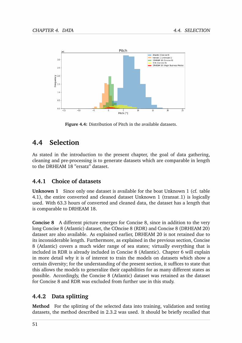
The aim of the present study consists in developing accurate forecasting models ofthe features that define the boat state as listed in section 2.4.1, as well as to conductexperiments with respect to the performance of these models for different boats anddatasets. This chapter presents the data available for this purpose.
4.1 Gathering
As described in section 2.2, new navigation logs have become available in the nke-proprietary format .nkz, in which data from boat sensors is recorded at 25 Hz.Datasets to be received in future iterations of JTR AI are going to be in this spe-cific format. The conversion of these files into .csv files that are usable by standardprogramming libraries is done with the software LogAnalyser and was described byRoman Kastusik in his thesis ([4]). This section describes the unforeseen challengesthat this data presented, which is always a risk with real world data.
4.1.1 Challenges encountered
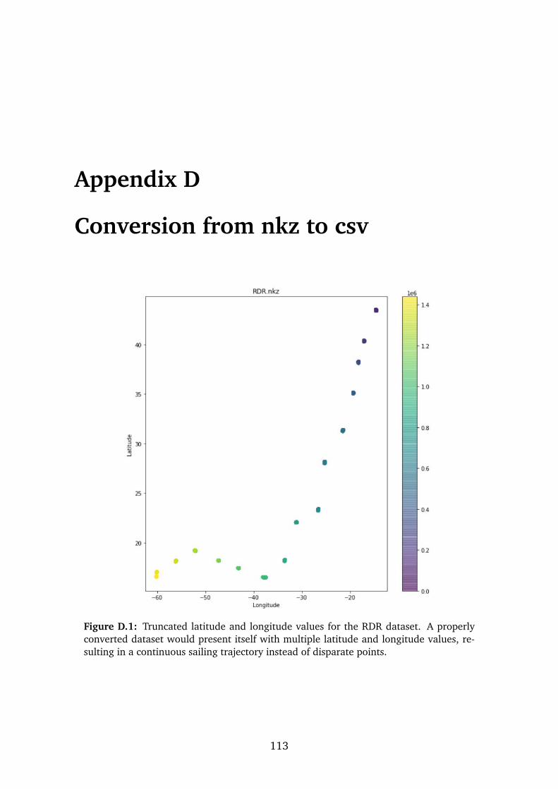
Description of main challenge However, a persistent problem occurred with theconversion of the new, .nkz-based files to the usable .csv format. Indeed, for thelatitude and longitude features, the conversion resulted in their values correspond-ing only to a very reduced set of values, as with a precision of 16 decimal placeswere expected and necessary. An example of a sailed trajectory consisting of thesetruncated latitude and longitude values is given in Appendix D.
Implications for the present study Only at the beginning of August 2020 andafter a lengthy exchange with nke could the correct conversion procedure be estab-lished. This unforeseen challenge added considerable overhead, affecting the scopeof the study. It should be emphasised that the resolution of this issue was not onlyof primordial importance for the present study, but also for future iterations of JTRAI, as there is no other way to obtain the navigation logs from the nke autopilots.
45
4.1. GATHERING CHAPTER 4. DATA
Further challenges It can generally be stated that the logging of the navigationdata by the nke autopilot is not consistent between boats. This concerns the numberof features recorded, which can vary from recording to recording. Furthermore, theorder in which the features are logged can also change from file to file. Hence, atopof requiring substantial computational and time resources, the conversion from .nkzto .csv files is tedious and requires multiple manual interventions.
4.1.2 Implications on conversion of datasets
Entirely converted datasets The datasets for which pre-processing and conversionwas successful are
• Atlantic
• RDR
• DRHEAM 20
They were hence entirely converted. This was also performed in view of futureiterations of JTR AI for which this data is likely to be valuable.
Partially or un-converted datasets However, the conversion process was particu-larly time consuming for the following datasets:
• transat 1 (Unknown 1)
• transat 2 (Unkown 2)
The conversion required multiple interventions to convert the .nkz files to .csv.Hence, in an effort to limit the resources devoted to this data gathering aspect ofthe study, it was decided to convert only a part of this data.
Determination of necessary dataset volume The overall objective of the presentstudy should be kept in mind, which consists in the identification of hyperparametersof reliable forecasting models for boat state features. This includes an assessment asto whether these hyperparameters are adequate for models trained on different dataformats (i.e. old DRHEAM 18 format vs. new .nkz-based format). It also includesthe assessment as to whether the hyperparameters are adequate for models trainedon datasets of the same format, but of different boats (e.g. Concise 8 and Unknown1). For the latter, it is sufficient to have one other boat than Concise 8; this boat waschosen to be Unknown 1 (transat 1). Furthermore, for these analyses it is sensibleto use comparable datasets, where comparability includes the mere volume of thedatasets. Hence, it suffices to convert only as much of transat 1 as is needed tohave a dataset length that is comparable to the length of cleaned data available forDRHEAM 18’s, i.e. 64.5 hours (as inherited from previous iterations of JTR AI, cf.
46
CHAPTER 4. DATA 4.2. CLEANING
2.2). The number of hours that is necessary to obtain a comparable length aftercleaning was found to be 67 hours, as is listed in table 4.1. The already brieflymentioned cleaning process of the converted data is explained in the next section.
4.2 Cleaning
Irrelevant data As explained in detail in section 2.3.1, it is of advantage not totrain an ML algorithm (whether supervised or RL-based) on segments with certainundesirable characteristics. These include
• tack maneuvers
• abnormal conditions which are irrelevant for racing (e.g. low wind speed)
• corrupted recordings with incomplete data
• segments where the boat was anchored or in the harbour, i.e. without anysailing being performed
Motivation Indeed, JTR AI focuses on improving the behaviour of the autopilotonly when it is engaged in normal sailing. Hence, data with the mentioned charac-teristics is not of relevance for the present study and needs to be removed from thedataset.
Cleaning procedure Hence, following the approach explained above in section2.3.2, the converted data was subdivided into segments of 60 seconds. The datawas examined for the mentioned undesirable characteristics, segment by segment.If such characteristics were detected, the corresponding segment was noted and notretained for further use. The result is shown in table 4.1. The following observationscan be made:
• For the Concise 8 (Atlantic) dataset of Concise 8, 228.7 hours are left aftercleaning, which is much more than required a priori.
• 16 more hours of data from Concise 8 is available from RDR.
• 63.3 hours of the new converted data remain for Unknown 1, which is only 1.2hours less than the number of hours recorded for DRHEAM 18 (64.5 hours)and hence of a comparable length.
• For VMB (DRHEAM 20) only 6 hours remain, because the boat was in a harbourduring one of the recorded 7 hours.
At this point it should be emphasised that in Roman Kastusik’s, the available datadid not pass through these pre-processing steps. Hence, his state estimator was alsotrained on segments containing tacks or low wind speeds, which is not desirablefor the reasons mentioned in section 2.3.1. This is a first clear difference to Roman
47
4.3. DISTRIBUTION CHAPTER 4. DATA
Kastusik’s approach.
After this cleaning of irrelevant segments, a look at the data provides informationabout the material available, which finally allows to make a selection of the datasetsto be used.
Boat Name Original Converted Cleanedlength [h] length [h] length [h]
Table 4.1: Overview of the original length, converted length and the cleaned length ofthe datasets available for the different boats.
4.3 Distribution
The goal of the present study consists in identifying hyperparameters of reliableforecasting models of the boat state features. Furthermore, it is attempted to assesswhether these hyperparameters are adequate for different formats of the datasetsand for models trained on different boats.
Motivation The selection of those data on which these forecasting models aretrained and of those on which their performance is tested is a cardinal step in thisprocess. Indeed, reliable forecasting models should capture the physics of the boatreliably for as broad a distribution of sailing conditions as possible.
Features describing the physical environment Only some features are relevantto describe the physical environment and state of the boat. Indeed, some featuresare partially redundant to others and some correlate strongly to others (e.g. boatand wind speed under normal conditions). Therefore, 4 features were selected thatcapture the essential elements of the environment as experienced by the boat. Inconsultation with Dr. Eric Topham, internal supervisor of the study with extensivesailing experience, these features were found to be:
• True Wind Speed (TWS): important for the lift generated from the airflowover the sails, as well as affecting the sea state.
• True Wind Angle (TWA): the angle at which the wind hits the boat in relationto its orientation when the boat would be stationary. It allows to characterizethe angle of the wind in relation to the boat at any given moment.
48
CHAPTER 4. DATA 4.3. DISTRIBUTION
• Apparent Wind Angle (AWA): characterizes the angle at which the wind ef-fectively hits the boat when the boat is in motion.
• Pitch: describes the inclination of the boat’s bow; numerous high and lowvalues for pitch hence indicate an agitated sea that would raise and lower thenose of the boat. Out of the pitch, roll and yaw angles that describe the attitudeof the boat, pitch is the best for approximating the sea state. Indeed, roll canbe affected by wind which can be independent of the sea state, and yaw can beaffected by the helmsman steering the boat in a choice of direction unrelatedto the sea state.
The distribution of these features’ values is described in figures 4.1 to 4.4 for thecleaned datasets. The following observations can be made:
• What is presented in visual form here corresponds to what can already be seenin table 4.1, namely that the datasets differ in their sheer volume: DRHEAM 20contains 6 clean hours, while Concise 8 (Atlantic) has almost 229 clean hours.
• Accordingly, the longer datasets cover a greater variety of conditions. This isreflected by the fact that for the shown key features, Concise 8 (Atlantic) coversvalues from almost all areas and also contains e.g. the rare moments wherevery high True Wind Speeds prevail (fig. 4.1), while DRHEAM 20 contains onlythe values specifically found during the 6-hour recording period.
• Finally, it can be noted that in fig. 4.2, True Wind Angles are also found insuboptimal angles close to -180° and 180° (suboptimal according to the polarplot 2.5). This can be explained by the fact that Concise 8 (Atlantic) was asingle-handed delivery, meaning that the autopilot was switched on over longdistances, while the other datasets were recorded during double-handed races,where a person was usually behind the tiller (cf. section 2.2). The standardautopilot just follows a given compass heading without adapting its behaviourto the TWA like a human would. Indeed, if the true wind direction remainschanged anfd the boat heading remains fixed, then the boat will experience achange in true and apparent wind angles resulting in the sailing under subop-timal wind angles.
49
4.3. DISTRIBUTION CHAPTER 4. DATA
Figure 4.1: Distribution of True Wind Speed (TWS) in the available datasets.
Figure 4.2: Distribution of True Wind Angle (TWA) in the available datasets.
Figure 4.3: Distribution of Apparent Wind Angle (AWA) in the available datasets.
50
CHAPTER 4. DATA 4.4. SELECTION
Figure 4.4: Distribution of Pitch in the available datasets.
4.4 Selection
As stated in the introduction to the present chapter, the goal of data gathering,cleaning and pre-processing is to generate datasets which are comparable in lengthto the DRHEAM 18 ”ersatz” dataset.
4.4.1 Choice of datasets
Unknown 1 Since only one dataset is available for the boat Unknown 1 (cf. table4.1), the entire converted and cleaned dataset Unknown 1 (transat 1) is logicallyused. With 63.3 hours of converted and cleaned data, the dataset has a length thatis comparable to DRHEAM 18.
Concise 8 A different picture emerges for Concise 8, since in addition to the verylong Concise 8 (Atlantic) dataset, the COncise 8 (RDR) and Concise 8 (DRHEAM 20)dataset are also available. As explained earlier, DRHEAM 20 is not retained due toits inconsiderable length. Furthermore, as explained in the previous section, Concise8 (Atlantic) covers a much wider range of sea states; virtually everything that isincluded in RDR is already included in Concise 8 (Atlantic). Chapter 6 will explainin more detail why it is of interest to train the models on datasets which show acertain diversity; for the understanding of the present section, it suffices to state thatthis allows the models to generalize their capabilities for as many different states aspossible. Accordingly, the Concise 8 (Atlantic) dataset was retained as the datasetfor Concise 8 and RDR was excluded from further use in this study.
4.4.2 Data splitting
Method For the splitting of the selected data into training, validation and testingdatasets, the method described in 2.3.2 was used. It should be briefly recalled that
51
4.4. SELECTION CHAPTER 4. DATA
this method consists of considering contiguous segments between two anomalies orbetween two tacks, and for each of those segments assign the first 60% of the datato the training subset, the next 20% to the validation subset and the last 20% to thetesting subset, as opposed to taking this split just once over the entire dataset. Fig.4.5 to 4.11 show the resulting distribution of the previously mentioned key sea statefeatures for the dataset Unknown 1 (transat 1), now divided into training, validationand testing subsets.
Resampling for large datasets However, performing this step for Concise 8 (At-lantic) does not affect its consisting of almost 229 (cleaned of tacks and anomalities)hours, which is considerably more than the ca. 65 hours of data which are deemednecessary at all. Hence, only a subsample of the training, validation and testing splitswas retained with a total duration of 63.3 hours, i.e. exactly the same amount asis available for Unknown 1. Hence, after splitting the data into training, validationand testing subsets just as for the transat 1 dataset, the subsets were each dividedinto 5 parts, respectively. For each of the subsets, only the first 27.7 % from eachof these 5 parts were retained and concatenated, so that the desired 63.3 hours oftotal training, validation and testing data were obtained. Fig. 4.6 to 4.12 show thedistribution of the subsets that were retained.
52
CHAPTER 4. DATA 4.4. SELECTION
Figure 4.5: Distribution of True Wind Speed in Unknown 1 (transat 1).
Figure 4.6: Distribution of True Wind Speed in Concise 8 (Atlantic).
Figure 4.7: Distribution of True Wind Angle in Unknown 1 (transat 1).
53
4.4. SELECTION CHAPTER 4. DATA
Figure 4.8: Distribution of True Wind Angle in Concise 8 (Atlantic).
Figure 4.9: Distribution of Apparent Wind Angle in Unknown 1 (transat 1).
Figure 4.10: Distribution of Apparent Wind Angle in Concise 8 (Atlantic).
54
CHAPTER 4. DATA 4.5. PREPROCESSING
Figure 4.11: Distribution of Pitch in Unknown 1 (transat 1).
Figure 4.12: Distribution of Pitch in Concise 8 (Atlantic).
4.5 Preprocessing
The data, cleaned and selected as described in the previous sections, must still beprepared before it can be fed into any models. This concerns firstly their content,i.e. mathematical transformations applied to the data, and secondly the form, i.e.re-arranging the data into a format that is compatible with the common ML-libraries.
4.5.1 Normalisation
Motivation Typically, the values of features are subject to rescaling before enteringdeep neural networks. This normalisation step allows to reduce the effects thatthe features’ different value ranges (cf. table 2.4) have on the performance of theneural networks employed. Furthermore, if a single model is to be trained to predict
55
4.5. PREPROCESSING CHAPTER 4. DATA
multiple values, the error metric that it is trained to optimise consists of the averageof the different feature’s prediction errors. Hence, if the models were to be trainedon unscaled data, the value of this overall error metric would be severely dependenton features whose value range can be relatively high (e.g. True Wind Direction),which would overtrump the effect of features that can only attain relatively lowvalues (e.g. Current Speed).
Transformations Table 4.2 provides an overview of the preprocessing applied tothe values of each feature, here can correspond to one of three transformations:
• As motivated and explained in detail in section 2.3.1 above, the sine and co-sine of the angle features is computed if their range covers [-180°,180°] or[0°,360°], effectively reducing their range to [-1,1].
• Features that can only take on positive values (e.g speed) are subject to Min-Max normalisation, i.e. xnormalised =
xoriginal−xminxmax−xmin . The normalised values hence
lie in the range [0,1].
• Features whose values might be either positive or negative (e.g. rudder angle,whose values are contained in the range [-45°,45°]) are subject to Max-Absnormalisation, i.e. xnormalised =
xoriginalmax(|xmin|,|xmax |)
. This leads to the normalisedvalues lying in the interval [-1,1].
4.5.2 Rearranging the Timeseries
As explained in detail in section 2.4.1, the timeseries data needs to be re-arrangedinto a specific format in order to enter the keras models. This step is conducted asthe last pre-processing intervention. While it has been described extensively in thementioned paragraph 2.4.1, a technical remark is opportune at this point.
Previous approach and disadvantages In previous iterations of JTR AI, the re-arranging of the data was done using a custom-made function (cf. [4], [5], [6]).This is error-prone and leads to the local runtime running out of memory for largedatasets.
Updated approach and advantages Hence, in the present study this step was con-ducted using the ”Timeseries Generator” class of TensorFlow. It relies on a generatorthat produces batches of timeseries data on which the models can be trained batchby batch. It has been specifically designed to transform timeseries data and to copewith large amounts of them. Apart from removing memory issues and error sources,the use of generators during model training allows for multi-processing, speeding upthe training process. The interested reader finds further information in the onlineTensorFlow documentation [35]. The use of this class might be of special interestfor future iterations of JTR AI.
56
CHAPTER 4. DATA 4.5. PREPROCESSING
Feature Name Range Preprocessing
Latitude [-90, 90] Max-Abs
Longitude [-180, 180] Cos and Sin
TWS [0, 40.0] Min-Max
TWD [0, 360] Cos and Sin
Current speed [0,15.0] Cos and Sin
Current direction [0, 360] Cos and Sin
Air temp [0, 30.0] Min-Max
Speed ov surface [0, 25.0] Min-Max
Speed ov ground [0, 25.0] Min-Max
VMG [0, 25.0] Min-Max
Heading True [0, 360] Cos and Sin
Heading ov ground [0, 360] Cos and Sin
Pitch [-20, 20] Max-Abs
Roll [-60, 60] Max-Abs
Yaw [-180, 180] Cos and Sin
AWS [0, 50.0] Min-Max
AWA [-180, 180] Cos and Sin
TWA [-180, 180] Cos and Sin
Rudder [-30, 30] Max-Abs
Table 4.2: Preprocessing applied to the features.
57
Chapter 5
Models
The aim of the present study is to develop reliable timeseries forecasting models forthose features that define the state of the boat, which is a supervised learning task.These forecasting models constitute the simulation environment for an RL agent thatis to learn to intelligently set the rudder angle. Hence, the only boat variable that isnot to be predicted by any supervised model and for which no model is investigatedhere is that of the rudder angle, as this feature is to be learnt by an RL agent.Different forecasting models are conceivable to predict the boat state features. Thepresent chapter presents the general structure and functioning of these models.
5.1 1 Model for n Features
Design A single model can be trained to predict the next values of all of the boatstate’s features. The single model receives as input the values of the n0 time stepspreceding the moment for which it is to make a prediction. The model returnsa vector of all predicted feature’s values. This model and the hyperparameters thatgovern it have been described and illustrated extensively in the background researchabove (2.4.1).
Advantages It is worth noting that the tuning of these hyperparameters allows toadapt the model’s behaviour and hence to optimise its performance for a given task.As described in detail in the background research above (2.3.3), Bayesian optimi-sation allows to improve the hyperparameters. The main advantage of training 1model for n features resides in this optimisation only being required for 1 model.Indeed, as the optimisation of hyperparameters can prove lengthy and tedious, con-ducting it for one model can be preferable over performing it for multiple models.This latter approach of training multiple models for timeseries forecasting problemat hand is described subsequently.
58
CHAPTER 5. MODELS 5.2. N MODELS FOR N FEATURES
5.2 n Models for n Features
Design The boat state consists of multiple features, each of which needs to bepredicted in timeseries prediction problem at hand. An alternative to training asingle model to predict n features’ values is to train n models separately. In thisframework, each model is trained to specifically predict only one variable’s nextstate; i.e. one model to predict the true wind speed, one model for apparent windangle, etc. The general structure of these models and the hyperparameters that canbe varied are identical as for the 1 model for n features, except that a single value isreturned instead of a vector constituting the predicted boat state. Hence, each of then models returns only one value. In turn, the n models together returning n valuesconstitute the RL simulation environment.
Advantages One advantage of this approach resides in the fact that the n modelsonly need to be optimised with respect to their respective features, instead of beingoptimised to predict all features at once. This reduces the complexity the modelsmust take into account.
5.3 Deterministic models
A radically different approach can also be adopted to compute the values of fea-tures. Indeed, the navigation logs contain directly measured values as perceivedby the sensors on board, e.g. Apparent Wind Angle (AWA), Apparent Wind Speed(AWS) etc. On the other hand, they contain values derived from these measuredvalues, such as the True Wind Angle (TWA) and the True Wind Speed (TWS). Thisderivation is done directly on board by the software of the nke autopilot and storedas such in the navigation logs. Table 2.4 lists feature by feature which features aredirectly measured and which are derived.
5.3.1 Motivation
Hence, it is possible to derive the values of certain features directly from the valuesof other features. This can be interesting for a number of reasons:
1. Alternative to forecasting models with poor performance: if no accurateforecasting model can be identified for a given feature, it might be computedfrom a number of other predicted values that can be accurately predicted. Thatway, a much more accurate estimate can still be computed, despite there notbeing an accurate LSTM-based model. An example of this is the TWA, which isdefined as a function of other features.
2. Evaluating the accuracy of data: If features are defined as direct functions ofeach other, the calculated values should in theory exactly match the recorded
59
5.3. DETERMINISTIC MODELS CHAPTER 5. MODELS
values, if they are computed on the basis of recorded, ”true” values (instead ofwhich one could also use predicted values, if one wants to make a prediction).In this sense, any discrepancies between the calculated and recorded valuesare an indicator of imperfections in the recorded values, because in the case ofexactly recorded values both should be exactly the same. This is of importanceas the sensors on board can potentially be poorly or mis-calibrated. Comparingthe recorded vs. the ”true” values recorded by the sensors and calculating thecorresponding error measures allows for a type of ground truth against whichto assess how strong such mis-calibrations potentially are.
3. Speed: this approach is potentially faster than providing inputs to a trainedLSTM-based model, performing the large number of calculations that thatmodel consists of, and only then having an output. Indeed, if relying partlyon first-principles formulae for the simulation environment, only some valueswould need to be predicted using the computationally heavier models, whilethe rest can be quickly determined using computationally light formulas. Itshould be noted that the speed of the predictions is not important in this study,since the goal is only to develop a reliable RL simulation environment. How-ever, in other applications, the speed at which predictions can be made mayplay a role. This will be explained in chapter 8.
5.3.2 Formulae
The exact derivation of the first-principles formulae will not be described here, asthis essentially corresponds to what has been described in the theses of Birk Ulstad[6], Roman Kastusik [4] and in various online resources, e.g. [36]. Here we will becontent to merely state the formulae for each of these features.
Definitions TWS and TWA are by their very definitions unambiguous functions ofother features:
• True Wind Angle (TWA):
TWAt+1,det = arccos(AWSt+1 · cos(AWAt+1)− Speed ov groundt+1
TWSt+1
)(5.1)
• True Wind Speed (TWS):
TWSt+1,det =(AWS2
t+1 + Speed ov ground2t+1
− 2 ·AWSt+1 · Speed ov groundt+1 · cos(TWAt+1)) 1
2(5.2)
It should be noted that TWA is a boat state feature as defined in section 2.4.1 above.It can hence be used in light of the first motivation stated above, i.e. to assesswhether it is theoretically possible to predict a given feature’s value by using otherfeatures. It can also be used with a view on the second motivation stated above,
60
CHAPTER 5. MODELS 5.3. DETERMINISTIC MODELS
i.e. to assess the accuracy of a dataset by comparing the computed and the recordedvalues. On the other hand, as defined in section 2.4.1, TWS is a sea state featureand not a boat state feature. It can hence only be used to assess the accuracy of thedataset, as the present study is concerned with identifying forecasting models forboat state features only.
Derivations For the latitude and longitude features, another first-principles basedmethod is used to derive the position of the boat in the next moment. Indeed, basedon the boat’s equations of motion, the position of the boat at the next instant t + 1can be calculated from certain values available at the current instant t. While theformulae governing the relationships of TWA and TWS and the other features are”absolute truths” that emanate from the definitions of these measures, the formulaeof latitude and longitude being derived from equations of motion means that theyare prone to slight deviations from the true recorded value. However, in the follow-ing, for the sake of conciseness both categories will be referred to as ”first-principles”or ”deterministic” formulae.
Definitions :
• Latitude:
Latitudet+1,det = arcsin(sin(Latitudet) · cos(Speed ov groundt/R)
+ cos(Latitudet) · sin(Speed ov groundt/R)
· cos(Heading ov groundt)) (5.3)
• Longitude:
Longitudet+1,det = Longitudet
+ arctan(sin(Heading ov groundt)
· sin(Speed ov groundt/R) · cos(Latitudet)+ cos(Speed ov groundt)/R)
− sin(Latitudet) · sin(Latitudet+1))
(5.4)
where the abbreviations for features are used as defined in table 2.4, and det indi-cates that a value is computed deterministically.
61
5.4. PREDICTION TIME HORIZON CHAPTER 5. MODELS
5.4 Prediction Time Horizon
At this point it should be noted that the models, just like in Roman Kastusik’s study,are to predict the boat variables in the next second. In other words, at a givenmoment t, a prediction is made of the boat state in the next instant t + 1s.
Choice of a time horizon Since the data was sampled at 25 Hz, i.e. every 0.04seconds, it would also be conceivable to predict the boat variables for any t+n·0.04s,where n is a strictly positive integer. Nonetheless, the ultimate goal of JTR AI is todevelop an algorithm that outputs an advantageous rudder angle that can be setby the autopilot hardware in the physical world. Now the live implementation ofall of collecting input data, calculating an adequate rudder angle and physicallysetting that rudder angle on board takes time. Indeed, this was the reason for oneof the major conclusions of a previous iteration of JTR AI [5], which consisted of therecommendation to focus on predictions for t + 1s instead of t + 0.20s.
Limitations and implications However, as explained in the background research2.3, 1s is also the most generous time horizon which should be used, as a humansailor is roughly estimated to change the rudder angle at least once per second. Forthese reasons, the prediction time horizon for the rudder prediction RL algorithmwas retained at 1 Hz, i.e. 1 second. The RL simulation environment - i.e. the time-series forecasting models discussed in the following - was hence also designed forthat time horizon, and the data needed to train, validate and test these models re-arranged to 1 Hz according to the procedure described in section 4.5.2.
5.5 Evaluation Metrics
Motivation The performance evaluation of the models is carried out using themean absolute error and the root mean squared error. Indeed, they are two eval-uation metrics commonly used in the machine learning community and allow toassess the performance of the models relatively quickly. While Roman Kastusik alsorelied on these two metrics to describe his model’s performance, the results are notdirectly comparable: in the mentioned thesis, different data was used and a differentpreprocessing was carried out. In particular, in Roman Kastusik’s work, data was notexamined for tacks or abnormal segments.
Definitions Finally, these two performance metrics are defined as:
• Mean absolute error (MAE):MAE = 1
n samples
∑n samplesi=1 |ytrue,i − ypredicted,i |
62
CHAPTER 5. MODELS 5.5. EVALUATION METRICS
• Root Mean Squared Error (RMSE):RMSE = 1
n samples
∑n samplesi=1 (ytrue,i − ypredicted,i)2
Now that there is clarity about both the available data and the models to be trainedand tested, the next chapter will explain the experiments that can be conducted withthem.
63
Chapter 6
Experiments
The overarching goal of this study consists in the identification of reliable forecastingmodels for the boat state features. This section presents the experiments conductedin view of that goal.
Overview The high-level approach adopted to resolving problem at hand can besubdivided into different steps, namely:
1. For a given boat’s dataset coming in a specific format, investigate whetheraccurate forecasting models can be identified. In the present study, Concise 8(DRHEAM 18) was retained for this step due to its being available early on inthe project.
2. Test whether the hyperparameters that are adequate for that boat and thatdataset’s format is also adequate for
• a dataset from the same boat, but in a different format, i.e. Concise 8(Atlantic).
• a dataset from a different boat and in a different format, i.e. Unknown 1(transat 1).
In the following sections, this approach is sub-divided into more fine-grained steps.
Motivation At this point it is worth explaining again why models with exactly thesame hyperparameters as found for DRHEAM 18 are trained on the new data. Theaim is to find out whether the hyperparameters identified for DRHEAM 18 from theold data format are also adequate for new, .nkz-based data formats for the same boat(Concise 8) and for a different boat (Unknown 1). In fact, if the latter was the case,this would mean that in order to generate a boat simulation environment, all that isneeded is a cleaned dataset that allows the model to learn different weights, but doesthis with the known hyperparameters. If this is not the case, it would mean that foreach new boat the architecture and hyperparameters would have to be optimised,which is a much more complex and time-consuming process than training modelswith a once-and-for-all identified architecture along an established pipeline. This is
64
CHAPTER 6. EXPERIMENTS 6.1. 1 MODEL FOR N FEATURES
of particular relevance as additional data from new boats is likely to be available infuture iterations of JTR AI.
Note about environment in which the experiments were conducted A cloud in-frastructure (Azure Machine Learning) was available for the experiments, with vari-ous different computing capacities (virtual machines) and correspondingly differentcomputing speeds. Most of the calculations were performed on a private laptop withan Intel Core i9-9980HK processor. All computing times that are indicated in thefollowing were recorded for the mentioned computer.
6.1 1 Model for n features
6.1.1 Motivation and Hypothesis
In a first approach, it was sought to improve the model that Roman Kastusik had de-veloped during his work on JTR AI and that was found to be inaccurate (cf. section2.4.1). This model consisted in 1 model for n features, consisting of 2 LSTM layersfollowed by 1 dense layer, as laid out in more detail in the background research 2.4.No optimisation of the hyperparameters was performed for this model. Hence, thisfirst step is concerned with verifying
Hypothesis 1: the performance of 1 model for n features can be improved byoptimising the model’s hyperparameters.
6.1.2 Experiments
Hence, the first experiment to conduct consists in optimising the model’s hyperpa-rameters. As laid out in the introduction of this chapter and summarised below intable 6.2,
• this optimisation is performed for the Concise 8 (DRHEAM 18) dataset thatwas recorded in a format that differs from the new, .nkz-based datasets.
• the single model for n features is then trained on the Concise 8 (DRHEAM 18)training subset and tested on its testing subset.
• the performance of the model is evaluated by considering the resulting testingerror metrics as well as samples of the predicted vs. the true values.
In the following sections, the approach for the optimisation of the hyperparametersis presented.
65
6.1. 1 MODEL FOR N FEATURES CHAPTER 6. EXPERIMENTS
6.1.3 Observed time window
A manual hyperparameter optimisation was conducted with respect to the observedtime, i.e. the number of time-steps whose values are fed into the LSTM layers, or inother words the number of time steps that the model is ”looking back”.
Choice of time window Indeed, after deliberations with the project’s supervisors,of whom Dr Eric Topham has extensive sailing experience, it was assumed that 60seconds of input would most probably be enough to capture the dynamics at sea(wind, waves, boat dynamics), while the original 100 seconds would be unnecessar-ily much.
Advantages of the chosen time window This has the considerable advantagethat the network’s weights only need to be trained for 60 inputs instead of 100,which in principle should entail a greatly reduced training time for the model toconverge. This is of particular importance as long training times can constitute amajor bottleneck for the progress of studies like the present one.
Potential for optimisation Naturally, the systematic and analytical optimisationof the input time window could be conducted. The literature presented above withe.g. [21] shows that this is an important area of interest currently. However, thegoal of the present study consists of the identification of hyperparameters that de-fine accurate forecasting models, as opposed to the analytical optimisation of theoptimal input time window length. Hence, in a first approach, it was refrained fromperforming an analytical optimisation of this hyperparameter.
6.1.4 Search space
The hyperparameters to be optimised are listed below in table 6.1. Before enunciat-ing any considerations as to how to optimise their values, it needs to be defined inwhat ranges to optimise these values.
Reasons for original model’s poor performance The main explanation for theoriginal hyperparameters’ resulting in unsatisfactory model performance is expectedto reside in its inability to capture the complex dynamics of the present problem.Indeed, if a single model is to predict n features for the highly dynamical systemrepresented by a sailboat, it must be able to capture the complexity of that task.
Dimensions of search space Hence, a relatively large search space should be cho-sen, in which combinations of hyperparameters are possible that take this complexityinto account. The search space that was adapted is hence characterised by generousdimensions, as can be seen in table 6.1. For instance, the batch size can vary from 64
66
CHAPTER 6. EXPERIMENTS 6.2. N MODELS FOR N FEATURES: MODEL 1
to eight times that value. Again, this large search space results from the fact that theprediction problem is considered rather complex and that any optimisation methodshould be allowed to take this complexity into account.
Hyperparameter Minimum Maximum OriginalBatch size 64 512 60Dropout rate 0.2 0.7 0.40Learning rate exponent -5 -1 -3Number of epochs 20 150 30Number of layers 1 6 2Number of nodes 10 51 50Observed time n0 [s] N.A. N.A. 100
Table 6.1: Search space for the hyperparameters of 1 model for n features, optimisedand original hyperparameters.
6.1.5 Bayesian Optimisation
Given the relatively large number of hyperparameters to be optimised, their optimi-sation by use of human experience as for the observed time window is out of thequestion. Hence, these hyperparameters were optimised by conducting a system-atic optimisation; namely by performing a Bayesian optimisation. This method andits advantages are presented above in the background research 2.3.3. It shall berecalled that its benefits reside in
• being computationally efficient, especially for large search spaces. This makesit preferable over other optimisation schemes like grid search, which requiresmany more iterations of models being trained and validated on different com-binations of hyperparameters, making it much more computationally costly.
• being able to optimise continuous hyperparameters (e.g. learning rate).Again, this stands in contrast to grid search, in which the models can only betrained and validated on discrete values.
Given this relatively large range of the search space, 25 steps of random explorationfollowed by 5 steps of Bayesian optimisation are conducted. This allows to effec-tively investigate a large proportion of the search space.
6.2 N models for n features: Model 1
6.2.1 Motivation and Hypothesis
As presented in detail in section 5.2, training n models separately to predict n fea-tures has the potential to yield better predictions. Indeed, each model only being
67
6.2. N MODELS FOR N FEATURES: MODEL 1 CHAPTER 6. EXPERIMENTS
required to learn the behaviour of ”its” feature is likely to yield more accurate than ifa single model has to capture all features’ behaviour together, with accuracy poten-tially suffering from the complexity of the task. Hence, this second step is concernedwith verifying
Hypothesis 2: training n separate models for n features yields more accuratepredictions than training 1 model for n features.
6.2.2 Experiments
Logically, this step is performed with the Concise 8 (DRHEAM 18) dataset, enablingcomparability with the single model for n features. As summarised below in table6.2, this approach consists in
• defining one set of hyperparameters that the n models are going to have,named ”Model 1”.
• training n models with Model 1 hyperparameters for the n features.
• evaluating the performance of the models by computing the testing error met-rics and comparing them with the results obtained with 1 model for n features.Furthermore, considering plots of samples of the predicted vs. true values al-lows to analyse the behaviour of the models and recognise poor behaviour (e.g.offset).
The choices for the Model 1 hyperparameters are explained in the following.
6.2.3 Model 1 hyperparameters
Motivation With unlimited time and computational resources available, the deter-mination of adequate hyperparameters for Model 1 would consist in the systematicoptimisation of the hyperparameters of each individual model. However, since theselengthy optimisations were out of the question in the present project, it was de-cided to train n models with the same hyperparameters in a first approach. If thehyperparameters entail unsatisfactory results for specific features, then these hyper-parameters can still be optimised in a second iteration.
Choice of hyperparameters In a first approach, the same hyperparameters as opti-mised for the single model for n features were retained, with one exception. Indeed,these hyperparameters are optimised for the same dynamics of the same boat butfor the prediction of multiple features. They can hence be taken as a valid startingpoint.
68
CHAPTER 6. EXPERIMENTS 6.3. N MODELS FOR N FEATURES: MODEL 2
Additional dense layer The Model 1 hyperparameters contain only one differenceto the set of hyperparameters that was optimised for 1 model for n features. Indeed,given the complexity of the present problem, one can argue that there only being onefinal dense layer does not take into account the complexity of the highly dynamicaland nonlinear problem at hand. However, in a deep learning model, dense layerswith relu activation functions increase a model’s ability to be trained on nonlineari-ties (cf. [34]). Hence, an additional dense layer with a relu activation function wasintegrated before the final dense layer for Model 1.
6.3 N models for n features: Model 2
6.3.1 Motivation and Hypothesis
Model 1 corresponds to one a standard set of hyperparameters for all n features.However, for some features, the additional dense layer of Model 1 can also be detri-mental to the model’s performance. Indeed, for those features which are not char-acterised by nonlinearities to the same degree as other features, it may be counter-productive to increase the model’s ability to capture nonlinearities (cf. [34]). Thisleads to the following
Hypothesis 3: if Model 1 hyperparameters lead to unsatisfactory results fora feature, removing one dense layer improves the prediction accuracy.
The set of hyperparameters identical to Model 1, but with only one final dense layeris dubbed ”Model 2” in the following.
6.3.2 Experiments
Again, this step is performed with the Concise 8 (DRHEAM 18) dataset, enablingcomparability with the single model for n features. As summarised below in table6.2, this approach consists in
• defining one set of hyperparameters that the models are going to have,named ”Model 2”.
• training the models for the selection of features.
• evaluating the performance of the models by computing the testing error met-rics and comparing them with the results obtained in the previous steps. Fur-thermore, considering plots of samples of the predicted vs. true values allowsto analyse the behaviour of the models and recognise trends in the behaviour.
Finally, while Model 2 is also a classical LSTM-based model, a radically differentapproach can also be taken to computing the values of certain features. This isexplained in the next section.
69
6.4. DETERMINISTIC MODELS CHAPTER 6. EXPERIMENTS
6.4 Deterministic models
6.4.1 Motivation and hypotheses
As explained in detail above in section 5.3, deterministic models potentially presenta number of advantages. Importantly, they might allow deriving some features’ val-ues directly from other features. These models are either a type of absolute truths(in the case of formal definitions) or derived from equations of motion. They arehence expected to result in better performance than LSTM-based models, which es-sentially have to learn the behaviour encapsulated in these formulae. This leads tothe following
Hypothesis 4: Where they can be used, deterministic models achieve betterperformance than LSTM-based models.
However, as laid out in detail in the mentioned section 5.3, the datasets themselvesmight contain imperfections resulting from e.g. sensor mis-calibration. This leads tothe following
Hypothesis 5: Where they can be used, deterministic models serve as an in-dicator of a dataset’s inaccuracies.
The viability of deterministic models is to be tested both for the old data formatof Concise 8 (DRHEAM 18), as well as for the new, .nkz-based data from Concise 8(Atlantic) as well as Unknown 1 (transat 1). Indeed, in view of the first hypothe-sis, this allows to assess whether these models can be applied to both data formats.Moreover, in view of the latter hypothesis, this enables to compare the quality of thedifferent datasets in function of their formats.
6.4.2 Experiments
The approach is summarised below in table 6.2; it consists in
• computing the values of TWA and TWS at moment t from the true values ofother features at moment t according to the deterministic formulae. Indeed,if perfectly accurate forecasting models were to be identified for the other fea-tures and TWA and TWS were to be computed from them, this constitutes thebenchmark performance that the prediction via direct derivation could achieve.Moreover, it allows to assess the quality of the data at hand, as the computedTWA and TWS should in theory exactly correspond to the true values.
• computing the values of Latitude and Longitude at moment t+1 from the truevalues at moment t. This allows to assess whether the first-principles model isa viable alternative to the LSTM-based models.
• evaluating the performance of the models by computing the testing error met-rics and comparing them with the results obtained in the previous steps (ob-
70
CHAPTER 6. EXPERIMENTS6.5. TRANSFERABILITY OF MODEL HYPERPARAMETERS
BETWEEN BOATS AND DATASETS
viously only for Concise 8 (DRHEAM 18)). Moreover, the consideration ofthese error metrics for TWA and TWS allows to assess the quality of the dataat hand. Furthermore, considering plots of samples of the predicted vs. truevalues allows to analyse the behaviour of the models and recognise trends inthe behaviour.
6.5 Transferability of model hyperparametersbetween boats and datasets
6.5.1 Motivation and hypotheses
The overarching goal of the present study consists in the identification of reliableforecasting models of the boat state features. The experiments from the previoussteps are designed to do so for one specific boat (Concise 8) and one specific datasetof a specific format (DRHEAM 18). As explained in detail in the introduction ofthis chapter, once these models have been identified for this specific combination ofboat and dataset, it is of crucial interest to see whether the hyperparameters of thesemodels are transferable. This leads to the following
Hypothesis 6: Hyperparameters of forecasting models that are accurate forConcise 8 (DRHEAM 18), i.e. the old data format, can be used to train accurateforecasting models using data from the same boat, but in the new, .nkz-basedformat (Concise 8 (Atlantic)).
This allows to evaluate the transferability of hyperparameters between differentdataset formats. In this light, another test can be made, namely
Hypothesis 7: Hyperparameters of forecasting models that are accurate forConcise 8 (DRHEAM 18), i.e. the old data format, can be used to train accurateforecasting models using data from a different boat and in the new, .nkz-basedformat (Unknown 1 (transat 1)).
This allows to evaluate the transferability of hyperparameters between differentboats with different dataset formats.
71
6.5. TRANSFERABILITY OF MODEL HYPERPARAMETERSBETWEEN BOATS AND DATASETS CHAPTER 6. EXPERIMENTS
6.5.2 Experiments
The verification of these hypotheses can be made by conducting the following exper-imental steps, as summarised in table 6.2:
• For each boat state feature, identify the best-performing model for Concise 8(DRHEAM 18).
• For Concise 8 (Atlantic) and Unknown 1 (transat 1), respectively:
– train n models for n features using the most accurate model’s hyperpa-rameters (from DRHEAM 18).
– evaluate the performance of the models by computing the testing errormetrics and comparing them with the results obtained in the previoussteps. Furthermore, considering plots of samples of the predicted vs. truevalues allows to analyse the behaviour of the models and recognise trendsin the behaviour.
72
CHAPTER 6. EXPERIMENTS6.5. TRANSFERABILITY OF MODEL HYPERPARAMETERS
BETWEEN BOATS AND DATASETS
Experiment 1: Optimise, train and test 1 model for n features
For the Concise 8 (DRHEAM 18) dataset:- Define search space in which hyperparameters of 1 model for n features
should be optimised- Perform Bayesian optimisation of hyperparameters- Compare optimised hyperparamaters to hyperparameters of original
1 model for n features- Train 1 model for n features with optimised hyperparameters- Test the trained model, compare with results obtained with
original model
Experiment 2: Train and test n separate models for n features
For the Concise 8 (DRHEAM 18) dataset:- Define 1 specific set of hyperparameters for the n models to be trained (Model 1)- Train n separate models (all with Model 1 hyperparameters) for all of the n
features- Evaluate for which features Model 1 is not satisfactory
Experiment 3: Tune, train and test selection of separate models
For the Concise 8 (DRHEAM 18) dataset:- Define 1 specific set of hyperparameters for those models for which Model 1
hyperparameters were not satisfactory (Model 2)- Train separate models (all with Model 2 hyperparameters) for that
selection of features- Evaluate for which features Model 2 is not satisfactory
Experiment 4: Test deterministic models
For the Concise 8 (DRHEAM 18),Concise 8 (Atlantic) and Unknown 1 (transat 1)datasets, respectively:
- For features for which deterministic models apply: compute valuesas function of other features
- Compare true and computed values to assess performance of deterministicmodels as well as accuracy of dataset
Experiment 5: Train and test n models for n features on new data
For the Concise 8 (Atlantic) and Unknown 1 (transat 1) datasets, respectively:- For each feature:
- If no deterministic model can be used, train model withhyperparameters that are most adequate according to DRHEAM 18 results
Table 6.2: Overview of the experimental approach.
73
Chapter 7
Results and Discussion
In the following, the results of the experiments are presented and discussed.
7.1 1 Model for n Features
7.1.1 Results
The following sections present the results of the optimisation, training and testing of1 model for n features. They correspond to the experimental steps laid out in section6.1 and summarised under Experiment 1 in table 6.2.
Bayesian Optimisation
The Bayesian optimisation required a total runtime of 6.5 days. Table 7.1 presentsthe Bayesian-optimised hyperparameters vs. the original hyperparameters. The op-timisation results in the same number of LSTM layers as the original model, namely2. All other hyperparameters change with respect to the original set of values.
Hyperparameter Optimised OriginalBatch size 88 60Dropout rate 0.387 0.40Learning rate exponent -3.21 -3Number of epochs 146 30Number of LSTM layers 2 2Number of LSTM nodes 35 50Overall MAE 0.048 0.062Overall RMSE 0.085 0.101
Table 7.1: Optimised and original hyperparameters of 1 model for n features. Over-all MAE and RMSE are with respect to the normalised feature values. Investigationsconducted with Concise 8 (DRHEAM 18).
74
CHAPTER 7. RESULTS AND DISCUSSION 7.1. 1 MODEL FOR N FEATURES
Training and Testing
Using the optimised hyperparameters as presented in the previous section, 1 modelfor n features was trained on the DRHEAM 18 training and validation subsets, whichtook a total of 12 hours. As can be seen in table 7.1, the 1 model for n featureswith optimised hyperparameters leads to an improved performance in comparisonto the original model trained by Roman Kastusik: the overall MAE of the normalisedvalues of the features is reduced from 0.062 to 0.048, and the corresponding RMSEis reduced from 0.101 to 0.085.
7.1.2 Discussion
It is found that the performance of the original model can be improved by conduct-ing a hyperparameter optimisation. Thus, the hypothesis laid out in section 6.1 isconfirmed.
Limitations of error measures However, the reader should be aware that as men-tioned in section 5.5, the performance metrics obtained here cannot be directly com-pared to the ones obtained for the original model, as the latter relies on differenttraining, validation and testing subsets. Hence, when performing comparisons withthis previous iteration of JTR AI, the values should only be considered as approxi-mate indicators of an overall improvement.
Bayesian optimisation It can be noted that the optimised hyperparameters resultin the same number of LSTM layers as the original architecture had. However, thenumber of LSTM nodes per layer is optimised from 50 to 35. This suggests thatthe model only needs to learn a reduced number of LSTM nodes and correspondingweights to capture the temporal dynamics of the boat (cf. [37] for further informa-tion on LSTM’s abilities to capture temporal patterns). This implies that the originalmodel exceeded the number of necessary nodes. Moreover, it is noted that the op-timised number of epochs increases nearly five-fold from 30 to 146, and that theoptimised batch size increases from 60 to 88. This indicates that the model needsto be trained longer and with more data as was the case with the original model.Hence, the original model was designed to capture an unnecessary level of temporalcomplexity in its 50 LSTM nodes, while not allowing for enough training in terms ofboth epochs and batch size.
Limitations of trained model Moreover, the achieved optimisation does not suf-fice to train a reliable forecasting model. Indeed, figs. 7.1 to 7.4 show an excerptof the course of the true values vs. the course of the predicted values for a selectionof features. It can be noted that in spite of the overall MAE and RMSE improvingwith the optimised architecture, the predictions made by the forecasting model donot accurately follow the true values. Indeed, if one considers the mentioned fig-ures, one can note that the 1 model for n values generally captures the up and down
75
7.1. 1 MODEL FOR N FEATURES CHAPTER 7. RESULTS AND DISCUSSION
movements of the features’ patterns. This pattern can be found similarly for all fea-tures; the presented selection of features and of the time window serves only as anexample.
Explanations for observed performance Furthermore, it can be noted that thefollowing of the true values does not happen on the correct scale, as well as witha strong offset. This suggests that the part of the model that allows to learn thechanges in time of the values, i.e. the LSTM layers, is able to capture the movementsin time of the values. Hence, the deficiency of the model is likely to reside in thepart of the model that transforms the LSTM’s output into the predicted value, i.e.the final dense layer with tanh activation function (cf. fig. 2.8 for the setup of theforecasting model).
Figure 7.1: Predictions for the sine of heading over ground (testing subset of DRHEAM18, Concise 8).
Figure 7.2: Predictions for apparent wind speed (testing subset of DRHEAM 18, Con-cise 8).
76
CHAPTER 7. RESULTS AND DISCUSSION 7.1. 1 MODEL FOR N FEATURES
Feature Name Model MAE RMSE
Longitude - cos 1 Model for n fatures 0.002 0.002
Model 1 0.002 0.002
Deterministic 5.783 · 10−7 5.445 · 10−7
Longitude - sin 1 Model for n fatures 0.029 0.035
Model 1 0.027 0.032
Deterministic 5.233 · 10−7 6.200 · 10−7
Speed ov surface 1 Model for n fatures 1.510 2.389
Model 1 1.200 1.846
Speed ov ground 1 Model for n fatures 1.530 1.938
Model 1 0.820 1.154
VMG 1 Model for n fatures 1.230 1.938
Model 1 0.520 0.866
Heading True - cos 1 Model for n fatures 0.042 0.072
Model 1 0.017 0.045
Heading True - sin 1 Model for n fatures 0.029 0.054
Model 1 0.017 0.038
Heading ov ground - cos 1 Model for n fatures 0.065 0.112
Model 1 0.037 0.076
Heading ov ground - sin 1 Model for n fatures 0.029 0.076
Model 1 0.020 0.044
Yaw - cos 1 Model for n fatures 0.017 0.061
Model 1 0.007 0.051
Yaw - sin 1 Model for n fatures 0.073 0.097
Model 1 0.040 0.053
TWA - cos 1 Model for n fatures 0.065 0.091
Model 1 0.026 0.036
Deterministic 0.746 0.938
TWA - sin 1 Model for n fatures 0.078 0.116
Model 1 0.021 0.034
Deterministic 0.745 0.938
Table 7.2: Test performance for the DRHEAM 18 dataset (Concise 8), part 1.
77
7.1. 1 MODEL FOR N FEATURES CHAPTER 7. RESULTS AND DISCUSSION
Feature Name Model MAE RMSE
AWA - cos 1 Model for n fatures 0.106 0.128
Model 1 0.028 0.037
AWA - sin 1 Model for n fatures 0.088 0.146
Model 1 0.021 0.037
Latitude 1 Model for n fatures 0.755 0.883
Model 1 0.835 0.955
Model 2 0.466 0.574
Deterministic 1.643 · 10−5 2.121 · 10−5
Pitch 1 Model for n fatures 0.720 0.950
Model 1 0.770 1.006
Model 2 0.641 1.058
Roll 1 Model for n fatures 2.940 4.047
Model 1 3.750 4.951
Model 2 1.390 2.002
AWS 1 Model for n fatures 2.340 3.136
Model 1 2.310 2.905
Model 2 1.220 1.748
Table 7.3: Test performance for the DRHEAM 18 dataset (Concise 8), part 2.
Figure 7.3: Predictions for pitch (testing subset of DRHEAM 18, Concise 8).
78
CHAPTER 7. RESULTS AND DISCUSSION7.2. N MODELS FOR N FEATURES:
MODEL 1
Figure 7.4: Predictions for latitude (testing subset of DRHEAM 18, Concise 8).
7.2 N Models for n Features:Model 1
The following sections present and discuss the results of the training and testing ofn separate models for n features. They correspond to the experimental steps laid outin section 6.2 and summarised under Experiment 2 in table 6.2.
7.2.1 Results
N models were trained for n features using the optimised hyperparameters and ar-chitectures with one additional dense layer as described in section 6.2 and as sum-marised in table 7.4. This took ca. 10.5 hours per feature, resulting in a total trainingtime of 19 features ·10.5 h
f eature = 199.5h for the training of all models.
Error metrics The resulting values for MAE and RMSE are listed in tables 7.2 and7.3. They are visualised in figs. 7.5 and 7.6. When comparing the prediction accu-racy obtained with Model 1 vs. the accuracy obtained with 1 Model for n features,the average change of the features’ MAE is -34.25 %, while the average change forRMSE is -32.57 %. It can be seen that both the MAE and the RMSE improve for allfeatures, the only exceptions are
• Latitude
• Pitch
• Roll
Furthermore, only a marginal improvement can be reached for the MAE of AWS(reduction of 1.28%).
79
7.2. N MODELS FOR N FEATURES:MODEL 1 CHAPTER 7. RESULTS AND DISCUSSION
7.2.2 Discussion
Accuracy of predictions Except for the 4 listed features, the improved error met-rics suggest a greatly improved performance of the n models for n features in com-parison to the 1 model for n features. Indeed, this is substantiated when consideringfig. 7.1. In the figure, it can be observed how the original and the predicted valuesstrongly agree for the example of the feature ”Heading over Ground”. This level ofperformance is also observed for all other features not listed above, i.e. satisfactoryforecasting models can be achieved for these features. For the features listed above,fig. 7.2 to 7.4 show by way of example that the performance of the Model 2 hyper-parameters is by no means satisfactory. Indeed, the predicted values hardly followthe tendencies of the true ones, i.e. they do not even capture the up and downmovements to a satisfactory degree.
Explanations for observed performance It can be observed that except for fourfeatures, the hyperparameters of Model 1 allow to capture the temporal patterns ofthe features. They do so without the offset observed for 1 model for n features, aswell as to scale. This is attributed to the fact that the n models can each tune theirweights to the behaviour of a single feature instead of being trained on predictingn features simultaneously. Furthermore, this is attributed to the additional denselayer being able to capture more nonlinear behaviour and the non-temporal aspectsof the model (cf. [34]), which was observed to be a problem in the evaluation ofthe previous experiment. A more detailed description of the effects of an additionaldense layer is laid out in 6.2.
Expressiveness of results It should be noted that with the present experimentalsetup, it cannot be quantified separately what the individual contributions are of theadditional dense layer as well as of the separate training of n models. As explainedin section 6.2 and as is clear from the nearly 200 hours required to train the models,this was not a priority in light of the temporal and computational resources of thepresent study. Moreover, the overall aim of the present study consists in the identifi-cation of reliable state estimators rather than in the systematic study of incrementalchanges to the hyperparameters. Hence, while one can note that the training of nseparate models with one additional dense layer leads to greatly improved forecast-ing models, the separate contributions of these two changes cannot be quantifiedhere.
In summary, the training of n separate models for n features yields more accuratepredictions than the single model for n features. The hypothesis laid out in section6.2 is thus confirmed. However, it is noted that for a reduced number of features,the separate models do not reach a satisfactory performance.
80
CHAPTER 7. RESULTS AND DISCUSSION7.2. N MODELS FOR N FEATURES:
MODEL 1
Hyperparameter Model 1 Model 2Number of LSTM layers 2 2Batch size 88 88Dropout rate 0.387 0.387Learning rate exponent -3.21 -3.21Number of epochs 146 146Number of Dense layers 2 1Number of nodes 35 35Activation function tanh tanh
Table 7.4: Hyperparameters of model 1 and model 2.
Figure 7.5: Change in MAE of Model 1 vs. 1 Model for n features (testing subset ofDRHEAM 18, Concise 8).
81
7.3. N MODELS FOR N FEATURES:MODEL 2 CHAPTER 7. RESULTS AND DISCUSSION
Figure 7.6: Change in RMSE of Model 1 vs. 1 Model for n features (testing subset ofDRHEAM 18, Concise 8).
7.3 N Models for n Features:Model 2
The following sections present and discuss the results of the tuning, training andtesting of separate models for a selection of features. They correspond to the exper-imental steps laid out in section 6.3 and summarised under Experiment 3 in table6.2.
7.3.1 Results
Model 2, which differs from Model 1 only in that it has one instead of two finaldense layers (cf. section 6.3), was trained on those features for which Model 1 hasproven to be insufficient. Its set of hyperparameters is summarised in table 7.4. Thetraining took ca. 9.5 hours per feature.
Error metrics As can be observed in table 7.3 and in figs. 7.7 and 7.8, the MAEand the RMSE decrease with Model 2 for all of the 4 concerned features. The onlyexcept is the RMSE for Pitch, which is more elevated than for 1 model for n features.
82
CHAPTER 7. RESULTS AND DISCUSSION7.3. N MODELS FOR N FEATURES:
MODEL 2
Figure 7.7: Change in RMSE of Model 2 vs. 1 Model for n features (testing subset ofDRHEAM 18, Concise 8).
Figure 7.8: Change in RMSE of Model 2 vs. 1 Model for n features (testing subset ofDRHEAM 18, Concise 8).
7.3.2 Discussion
Training time The training time per model is inferior to that observed for Model 1(9.5 hours vs. 10.5 hours). This is coherent with the fact that fewer weights need tobe trained without the 35 dense nodes from the removed dense layer.
Performance of models The performance of Model 2 for AWS and Roll is satis-factory, as emanates from the decreasing error metrics (cf. fig. 7.7 and 7.8) as wellas from fig. 7.2, presenting an excerpt for AWS. Removing one dense layer hence
83
7.4. DETERMINISTIC MODELS CHAPTER 7. RESULTS AND DISCUSSION
improved the performance of the forecasting models with respect to Model 1. This isattributed to the fact that the additional dense layer with relu activation function ofModel 1 leads to the model training for an excessive level of nonlinearity (cf. [34]).This effect is reduced by reducing the number of dense layers to one. Moreover, forPitch and Latitude, the picture is tainted: from fig. 7.3 it is obvious that the trainedmodel is able to predict the course of Pitch, but does not do so to scale. Moreover,considering the discrepancy between true and predicted values in fig. 7.4, it is isevident that the hyperparameters of model 2 do not deliver a reliable predictionmodel.
Observations for Pitch For Pitch, strong doubts can be expressed as to whetherthe pitch recorded in the DRHEAM 18 dataset can be considered accurate. Indeed,as can be seen in fig. 7.3, it remains at 0° to change only rarely and abruptly. Thiscorresponds to a boat that would pitch hardly at all and when it does, very stronglyat once. However, the inclination of a boat changes constantly when sailed, evenif perhaps only slightly. As will be seen in the following sections, this stands inopposition to the new, .nkz-based data, where Pitch is subject to strong changes(cf. fig. 7.21). The latter hence reflect the real conditions much more accurately.For these reasons, no further model for pitch was investigated in a first phase untilexperiments with the new, .nkz-based data.
Observations for Latitude Considering fig. 7.4, it can be stated that none of thetrained and tested models is satisfactory to predict Latitude. The predictions of themodels deviate strongly from the true values, not only on the shown excerpt, butalso concerning MAE and RMSE. While the detailed results can be found in tables7.2 and 7.3, one can note that e.g. the MAE of 0.466 degrees latitude corresponds inthe more frequently used units to 51.73 kilometers, which is obviously not satisfac-tory. However, in the first phase of experimentation, we refrained from investigatingalternative models to achieve better predictions of latitude. Indeed, in an attemptto optimise time and computation resources, it was decided to first consider the per-formance of deterministic models for Latitude before entering any hyperparameteroptimisations for the Latitude model.
In summary, for those features where Model 1 hyperparameters lead to unsatis-factory results, removing one dense layer improves the prediction accuracy. Thehypothesis laid out above in section 6.3 can hence be confirmed. However, for Pitchand Latitude, the improved accuracy is not at a satisfactory level.
7.4 Deterministic Models
The following sections present and discuss the results of the testing of deterministicmodels for a selection of features. They correspond to the experimental steps laidout in section 5.3 and summarised under Experiment 4 in table 6.2.
84
CHAPTER 7. RESULTS AND DISCUSSION 7.4. DETERMINISTIC MODELS
At this point, it should be emphasised that the following sections are presented witha rare shift from a boat-centric point of view to a dataset-centric perspective. In-deed, as laid out in 5.3, first-principles models can be used to assess the accuracy ofa dataset. Such an evaluation is hence inherently focused on datasets, and not onboats.
7.4.1 Results
Error metrics The resulting error metrics are presented in tables 7.2 and 7.3 forDRHEAM 18, table 7.6 for Atlantic and table 7.7 for transat 1. For DRHEAM 18, itcan be observed that the predictions made for both Latitude and Longitude presentover 99.9 % percent lower MAE and RMSE than obtained with the best LSTM-basedmodels. For Atlantic and transat 1, the error metrics are of a comparable low orderof magnitude. For the computation of TWS from other features’ true values, theerror metrics are in the same range: DRHEAM 18 presents an MAE of 0.461 knots,Atlantic an MAE of 0.410 knots and transat 1 an MAE of 0.230 knots. Finally, forTWA (split into cos and sin), both error metrics are ca. 30 times higher for DRHEAM18 than recorded for the best-performing LSTM model. For Atlantic and transat 1,the MAE and RMSE are in a comparable range as for DRHEAM 18.
7.4.2 Discussion
Performance for TWS The results presented above indicate that for both dataformats, the recordings for TWS are in strong accordance with the unambiguousformulae by which the different features are defined. Plots 7.9 to 7.11 illustrate theability of the deterministic model to closely follow the true values of TWS. However,as the MAE and the RMSE are not exactly zero as they should by definition, it shouldbe noted that the datasets cannot be considered as absolute ground truths. This isattributed to the sensors on board being mis-calibrated as well as to sensor drift thatmight occur in the rather harsh environment of the sea.
Performance for TWA As indicated by the error metrics TWA, the recordings arehardly in accordance with the deterministic formulae for TWA. Fig. 7.12 to 7.14display this for an illustrative excerpt. In other words, it is found that the TWA datacannot be considered as absolute truth.
Performance for Latitude and Longitude Finally, for Latitude and Longitude, itwas observed that the error metrics can be substantially reduced with respect to allother models for DRHEAM 18. Furthermore, it has been noted that they remain in acomparable order of magnitude for Atlantic and transat 1. Hence, the first-principlesformulae derived from the equations of motion provide a reliable forecasting modelfor these features.
85
7.4. DETERMINISTIC MODELS CHAPTER 7. RESULTS AND DISCUSSION
Illustration of Latitude and Longitude predictions Fig. 7.15 and 7.16 illustratethese results on a purely illustrative basis, i.e. without constituting any reference bywhich to judge the models’ performance. For a given starting point, the followingpositions are calculated by using each time
• the previous latitude and longitude, computed from the first-principles formu-lae
• values of the other features as required by the first-principles formula (truevalues as recorded in the dataset)
The resulting trajectories follow the originally recorded path relatively closely for thegiven, purely illustrative excerpt of 5 minutes of data. Even though at first glance thecalculated and recorded end positions seem to differ considerably for DRHEAM 18,the deviation between the coordinates of the two final points for the given examplecorresponds to 13.35 m over a total true . For Atlantic (final deviation of 2.17) andtransat 1 (final deviation of 3.83 m), the performance for these purely illustrativeexcerpts is comparable. Fig. 7.16 illustrates this behaviour for transat 1.
Hence, in summary, considering the True Wind Angle and DRHEAM 18, the de-terministic model does not provide better performance than LSTM-based models.The first hypothesis laid out in section 5.3 is hence partially refuted. Indeed, forTWS, Latitude and Longitude, the deterministic models are superior to the LSTM-based models. Hence, while it cannot be generally stated that the deterministicmodels always outperform LSTM-based models, for some features they do. Finally,when considering e.g. fig. 7.14 and the corresponding error metrics, the secondhypothesis made in section 5.3 can be confirmed: the deterministic models serve asindicators of a dataset’s inaccuracies.
Figure 7.9: Computed vs.true values for True Wind Speed (testing subset of DRHEAM18, Concise 8).
86
CHAPTER 7. RESULTS AND DISCUSSION 7.4. DETERMINISTIC MODELS
Figure 7.10: Computed vs.true values for True Wind Speed (testing subset of Atlantic,Concise 8).
Figure 7.11: Computed vs.true values for True Wind Speed (testing subset of transat 1,Unknown 1).
Figure 7.12: Computed vs.true values for True Wind Angle (testing subset of DRHEAM18, Concise 8).
87
7.4. DETERMINISTIC MODELS CHAPTER 7. RESULTS AND DISCUSSION
Figure 7.13: Computed vs.true values for True Wind Angle (testing subset of Atlantic,Concise 8).
Figure 7.14: Computed vs.true values for True Wind Angle (testing subset of transat 1,Unknown 1).
Figure 7.15: Computed vs.true latitude and longitude values for a 5 minutes excerpt(DRHEAM 18, Concise 8). The starting point is in the upper left corner, from where theboat was sailed to the lower right.
88
CHAPTER 7. RESULTS AND DISCUSSION 7.4. DETERMINISTIC MODELS
Figure 7.16: Computed vs.true latitude and longitude values for a 5 minutes excerpt(testing subset of transat 1, Unknown 1). The starting point is in the upper left corner,from where the boat was sailed to the lower right.
89
7.5. TRANSFERABILITY OF MODELS BETWEENBOATS AND DATASETS CHAPTER 7. RESULTS AND DISCUSSION
Feature Name Retained model Deterministic model
Longitude - cos Deterministic Yes
Longitude - sin Deterministic Yes
Speed ov surface Model 1
Speed ov ground Model 1
VMG Model 1
Heading True - cos Model 1
Heading True - sin Model 1
Heading ov ground - cos Model 1
Heading ov ground - sin Model 1
Yaw - cos Model 1
Yaw - sin Model 1
AWA - cos Model 1
AWA - sin Model 1
TWA - cos Model 1 Yes
TWA - sin Model 1 Yes
Latitude Deterministic Yes
Pitch Model 2
Roll Model 2
AWS Model 2
Table 7.5: Best-performing models for the boat state features according to the Concise 8 (DRHEAM18) dataset.
7.5 Transferability of models betweenboats and datasets
The following sections present and discuss the results of the training and testing ofn separate models for n features on new data. They correspond to the experimentalsteps laid out in section 6.5 and summarised under Experiment 5 in table 6.2.
The previous experimental steps served to identify optimised forecasting models forConcise 8 (DRHEAM 18). The models retained as best for the various features aresummarised in table 7.5. As previously presented, very accurate results were ob-tained with the deterministic models for Latitude and Longitude. Hence, in contrast
90
CHAPTER 7. RESULTS AND DISCUSSION7.5. TRANSFERABILITY OF MODELS BETWEEN
BOATS AND DATASETS
to all other features, no LSTM-based models were retained for these features.
7.5.1 Concise 8 (Atlantic)
Results
Error metrics Table 7.6 presents the error metrics that result from this experimen-tal step. Fig. 7.17 visualises the difference between the MAE values recorded forAtlantic and the ones obtained for DRHEAM 18 with the same model hyperparam-eters. A similar situation holds for the RMSE. The visualisation is performed onlyfor LSTM-based models, as the previous section already presents and discusses thedeterministic models.
Discussion
Performance The performance of the models is generally not comparable with thatfound for DRHEAM 18. Both the MAE and the RMSE increase in comparison to thevalues obtained for DRHEAM 18 for nearly all features, as can be seen in fig. 7.17for the MAE. A few exceptions can be observed; e.g. for AWS, the MAE and RMSE(1.211 and 1.484) are below the values found for the models trained and tested onDRHEAM 18 (1.220 and 1.748). The satisfactory performance for AWS is illustratedby the course of the predicted vs. true values as shown in fig. 7.20. However, asbecomes apparent from fig. 7.17, for the vast majority of features the quality of thepredictions differs considerably from those determined for DRHEAM 18. Fig. 7.19illustrates this for feature ”Heading over ground - sine”. While the predicted valuesfollow the pattern of the true values, a strong and consistent offset between bothcourses can be noticed. Finally, fig. 7.21 illustrates a similar behaviour for Pitch.While the mentioned figures are excerpts to illustrate the behaviour of the models,the same observations regarding poor performance hold for the other features.
In summary, the hyperparameters that result in accurate forecasting models forConcise 8 (DRHEAM 18) cannot be simply transposed identically to the trainingof forecasting models for the same boat, but with a different data format (Concise 8(Atlantic)). The first hypothesis laid out in section 6.5 is hence refuted.
91
7.5. TRANSFERABILITY OF MODELS BETWEENBOATS AND DATASETS CHAPTER 7. RESULTS AND DISCUSSION
Figure 7.17: Change in MAE of Atlantic vs. DRHEAM 18 (both for Concise 8). x-axiscut off at 600 % (% change for TWA - sin: 3271.43).
Figure 7.18: Change in MAE of transat 1 (Unknown 1) vs. DRHEAM 18 (Concise 8).x-axis cut off at 600 % (% change for TWA - cos: 1723.08, TWA - sin: 819.05, AWA -cos: 721.43).
92
CHAPTER 7. RESULTS AND DISCUSSION7.5. TRANSFERABILITY OF MODELS BETWEEN
BOATS AND DATASETS
Figure 7.19: Predictions for the sine of heading over ground (testing subset of Atlantic,Concise 8).
Figure 7.20: Predictions for apparent wind speed (testing subset of Atlantic, Concise8).
Figure 7.21: Predictions for pitch (testing subset of Atlantic, Concise 8).
93
7.5. TRANSFERABILITY OF MODELS BETWEENBOATS AND DATASETS CHAPTER 7. RESULTS AND DISCUSSION
Feature Name Retained model MAE RMSE
Longitude - cos Deterministic 1.398 · 10−7 1.647 · 10−7
Longitude - sin Deterministic 7.889 · 10−8 9.316 · 10−8
Speed ov surface Model 1 0.834 0.986
Speed ov ground Model 1 0.887 1.095
VMG Model 1 1.098 1.378
Heading True - cos Model 1 0.027 0.034
Heading True - sin Model 1 0.089 0.112
Heading ov ground - cos Model 1 0.060 0.072
Heading ov ground - sin Model 1 0.047 0.062
Yaw - cos Model 1 0.006 0.009
Yaw - sin Model 1 0.071 0.087
TWA - cos Model 1 0.175 0.251
Deterministic 0.746 0.939
TWA - sin Model 1 0.0373 0.0560
Deterministic 0.708 0.938
AWA - cos Model 1 0.163 0.183
AWA - sin Model 1 0.036 0.054
Latitude Deterministic 3.994 · 10−5 4.033 · 10−5
Pitch Model 2 2.477 2.993
Roll Model 2 7.242 8.452
AWS Model 2 1.211 1.484
Table 7.6: Test performance for the Concise 8 (Atlantic) dataset.
7.5.2 Unknown 1 (transat 1)
Results
Error metrics Table 7.7 presents the error metrics resulting from this final exper-imental step. Fig. 7.18 visualises the difference between the MAE recorded fortransat 1 and for DRHEAM 18 with the same model hyperparamaters. It can be ob-served that the MAE increases for all features except for Speed over Surface, cosineof Yaw and sine of Yaw.
94
CHAPTER 7. RESULTS AND DISCUSSION7.5. TRANSFERABILITY OF MODELS BETWEEN
BOATS AND DATASETS
Discussion
Performance Similarly to the results obtained for Atlantic, the performance of themodels is generally not comparable to the one found for DRHEAM 18. By consid-ering fig. 7.18, one can observe that the MAE increases for nearly all features; thesame holds for the RMSE. As observed for Atlantic, for some features, the error met-rics are comparable or improve with respect to the metrics observed for DRHEAM18. Among these is the cosine of Yaw, for which the MAE passes from 0.007 to0.0007 and the RMSE from 0.061 to 0.001. However, when considering fig. 7.18, itis evident that this is an exception and that the majority of the hyperparameters thatare adequate for DRHEAM 18 are not for transat 1. Furthermore, figs. 7.22 to 7.24again reveal the same pattern that can be observed as for Atlantic (Concise 8): whilethe models capture the time element of the patterns rather consistently, i.e. followthe up and down movements of the true values, they do so with a strong offset andnot to scale.
Similarities with Atlantic By comparing figs. 7.17 and 7.18, one can observe thatthe change in for Concise 8 (Atlantic) and transat 1 (Unknown 1) is negative or closeto zero for a number of features. Interestingly, this selection of features is similar forboth datasets, namely for the features Speed over Surface, Speed over Ground andcosine of Yaw.
Implications of similarities This means that for some features, the hyperparam-eters found for DRHEAM 18 are adequate. For these features, the hyperparametersdo generalise to data recorded for the same boat in a different data format (Concise8 (Atlantic)), as well as to data recorded for different boats in a different data for-mat (Unknown 1 (transat 1)). Hence, it cannot be excluded that at least for somefeatures, optimised hyperparameters might be transferred between data formats andboats.
In summary, the hyperparameters that result in accurate forecasting models forConcise 8 (DRHEAM 18) cannot be simply transposed identically to the trainingof forecasting models for a different boat with a different data format (Unknown 1(transat 1)). The second hypothesis laid out in section 6.5 is hence refuted.
95
7.5. TRANSFERABILITY OF MODELS BETWEENBOATS AND DATASETS CHAPTER 7. RESULTS AND DISCUSSION
Figure 7.22: Predictions for the sine of heading over ground (testing subset oftransat 1, Unknown 1).
Figure 7.23: Predictions for apparent wind speed (testing subset of transat 1, Un-known 1).
Figure 7.24: Predictions for pitch (testing subset of transat 1, Unknown 1).
96
CHAPTER 7. RESULTS AND DISCUSSION7.5. TRANSFERABILITY OF MODELS BETWEEN
BOATS AND DATASETS
Feature Name Retained model MAE RMSE
Longitude - cos Deterministic 1.384 · 10−7 1.762 · 10−7
Longitude - sin Deterministic 3.811 · 10−7 4.743 · 10−7
Speed ov surface Model 1 1.002 1.152
Speed ov ground Model 1 0.981 1.145
VMG Model 1 2.377 2.875
Heading True - cos Model 1 0.046 0.076
Heading True - sin Model 1 0.039 0.056
Heading ov ground - cos Model 1 0.058 0.092
Heading ov ground - sin Model 1 0.028 0.041
Yaw - cos Model 1 0.0007 0.001
Yaw - sin Model 1 0.035 0.045
TWA - cos Model 1 0.474 0.656
Deterministic 0.369 0.390
TWA - sin Model 1 0.193 0.273
Deterministic 0.549 0.564
AWA - cos Model 1 0.230 0.272
AWA - sin Model 1 0.053 0.080
Latitude Deterministic 4.838 · 10−5 4.977 · 10−5
Pitch Model 2 1.027 1.281
Roll Model 2 7.263 8.947
AWS Model 2 2.178 2.816
Table 7.7: Test performance for the Unknown 1 (transat 1).
97
Chapter 8
Conclusion and Future Work
The overarching goal of this thesis consists in developing reliable forecasting modelsfor features that describe the state of a sailing boat. The results presented aboveallow to draw a number of conclusions. Moreover, they allow to determine a clearframework with which to train reliable forecasting models and hence generate areliable RL simulation environment.
8.1 Conclusion
In the present study, it was shown that it is possible to identify reliable forecastingmodels for the features that define a sailboat’s state. It was found that trainingseparate models individually for all the features is an expedient method to that end.However, it was shown that the hyperparameters of these separate models do notgeneralise across different navigation recording systems. Finally, it could not beconclusively determined whether for a given data format, the hyperparameters offorecasting models generalise across different boats. Different conclusions can bedrawn from this.
1. As a first conclusion, Bayesian optimisation improves the performance of asingle forecasting model for n features (7.1). In comparison to the original,un-optimised model, the reduction of the overall MAE is of -22.58%, while theoverall RMSE is reduced by 15.84% However, the optimised single model doesnot achieve an accurate level of prediction performance. This is illustratedbelow in fig. 8.1, showing an excerpt of one of the features’ true and predictedvalues. The poor performance attributed to the fact that a single networkcannot take into account the complexity of the task at hand.
2. Using the Concise 8 (DRHEAM 18) dataset, it has been shown that it is possibleto train and test n reliable models for n features, and that they result in moreaccurate predictions than a single model for n features (7.2). Furthermore, it ispossible to do so with a relatively small amount of cleaned data (64.5 hours forDRHEAM 18). Only one exception holds, namely for Pitch ( 7.3.1). However,this was not investigated further as it is found that the data available for Pitchis highly likely to be corrupted. Finally, for the problem at hand, tuning the
98
CHAPTER 8. CONCLUSION AND FUTURE WORK 8.1. CONCLUSION
models by removing a dense layer proves successful (7.3) as it allows to adaptthe model’s ability to capture the level of nonlinearities effectively at hand([34]). This can be observed in fig. 8.1 below, where the tuning of a firstmodel (Model 1) leads to better results (Model 2).
3. It is found that for some features, deterministic models that rely on first-principles formulae can be used instead of LSTM-based models (7.4). Theyoutperform the latter for latitude and longitude (99.97% improvement or moreover best-performing LSTM models) and are a viable alternative to them. More-over, the use of deterministic formulae allows to conclude that the data at handdoes not represent the absolute physical truth and that it should be used withcaution. Indeed, the values of some features should be exactly derivable fromthose of other features, as they are linked by unambiguous formulae and arepartly calculated directly in that way in the autopilot software. It is hencefound that these formulae can serve as an indicator of a dataset’s inaccuracies.However, when verifying whether the recorded data is coherent with the unam-biguous relationships that govern this data, it was found that these computedvalues are not exactly identical with the recorded values. As an example, forthe Atlantic dataset, the values of AWS are computed by using the originallyrecorded ”true” data. The computed values for AWS show an MAE of 0.410knots to the originally recorded values for AWS, i.e. the formula is not exactlyverified. This inaccuracy is attributed to the mis-calibration of the autopilotsensors.
4. It is found that hyperparameters that lead to accurate results for a given dataformat do not generalise to other data formats (7.5). This was shown by usingdata that was recorded for the same boat, but relied on a different collectingsystem (Concise 8). It was also shown for data that was recorded for differentboats using different collecting systems (Concise 8 and Unknown 1).
Figure 8.1: Predictions for apparent wind speed (testing subset of DRHEAM 18, Con-cise 8).
Hence, in summary, reliable forecasting models of the boat state features could beidentified in the present study. However, they could only be established for a specific
99
8.2. FUTURE WORK CHAPTER 8. CONCLUSION AND FUTURE WORK
boat for which data is at hand in a specific data format (Concise 8 (DRHEAM 18)).This data format corresponds to an old recording protocol.
All of the new data available for this and future iterations of JTR AI is going to bein a modern .nkz format. Hence, the logical next step of JTR AI consists in optimis-ing and training forecasting models for different boats (Concise 8 and Unknown 1)using datasets in the .nkz format. This allows to assess the transferability of modelhyperparameters across different boats rather than across different data formats.This investigation constitutes the logical next step in reaching the overarching goalof the present study, i.e. creating a reliable RL simulation environment by identifyingaccurate forecasting models of the boat state’s features. From this, a framework forfuture work in JTR AI can be derived. It will be presented subsequently.
8.2 Future Work
8.2.1 Framework to create a reliable RL simulation environment
Motivation
The logical next step in JTR AI consists in the identification of reliable forecastingmodels for the boats state features. In particular, it would be of interest to identifyarchitectures and hyperparameters that allow the training of adequate forecastingmodels for any new .nkz dataset from any unseen boat.
Computational cost This would save the long and computationally intensive stepof identifying optimal models using Bayesian optimisation each time data from anew boat becomes available. Indeed, the Bayesian optimisation of 1 model for nfeatures alone required 6.5 days of runtime (cf. section 6.1).
Generalisability Besides the identification of generalisable architectures and hy-perparameters, it would be of interest to investigate whether there are generalisablemodels which, once trained, might be applicable to other boats of the same class(e.g. a model trained on Concise 8 (Class 40) which would be applicable to VMB(Class 40)), or which are trained on hybrid datasets and might be applicable to otherboats. An example of the latter would be a model trained on Concise 8 (Class 40)and Unknown 1 (IMOCA 60) which would be adequate for Unknown 2 (IMOCA 60).This would be the ”holy grail” of forecasting models for JTR AI, as the resulting RLsimulation environment would be suitable for any boat, which would mean that onewould only need to focus on developing the RL algorithms. Indeed, this would sig-nificantly increase the scalability and commercial viability of any solutions, as onewould not need to re-iterate through all optimisation steps each time an algorithmwould need to be developed for a new boat.
100
CHAPTER 8. CONCLUSION AND FUTURE WORK 8.2. FUTURE WORK
Framework
The framework to conduct this in a systematic manner is presented below in table8.1. It is based on the conclusions drawn from the present study and composed ofthe following steps:
1. individually optimise n models for n features. In 7.1, it has been shown thatBayesian optimisation can be used to improve a forecasting model. Moreover,
• it was found that the number of dense layers following the LSTM layersinfluences the behaviour of the forecasting models (6.2 and 6.3). Hence,the search space should include the number and width of dense layers ofthe network.
• this should be done for all features except Latitude and Longitude. In-deed, in section 7.4 it was found that the deterministic models can beused for accurate predictions with the available datasets.
• the optimised hyperparameters should be compared to identify whethercertain features require similar or even identical hyperparameters. Thisallows for extensions of research into the transferability of hyperparame-ters across the models for different boats.
2. train the models with the optimised hyperparameters.
3. test the trained models
• on the testing subset of the dataset they were trained on, such that itsperformance can be assessed.
• on the testing subsets of the other datasets to assess whether modelstrained on one boat generalise to other boats.
Data to be used
The described investigation should be conducted with the Concise 8 (Atlantic), theUnknown 1 (transat 1), and a hybrid dataset. The hybrid dataset should be sam-pled from training, validation and testing data from the Concise 8 (Atlantic) andUnknown 1 (transat 1) datasets. Indeed, the use of a hybrid dataset allows to assesswhether there are features for which models can be trained on data from differentboats and still result in accurate predictions. In other words, this helps to assesswhether there are features for which models can be trained boat-independently. Asexplained in the first part of this section, this would be beneficial by reducing thecomputational effort to train accurate forecasting models.
101
8.2. FUTURE WORK CHAPTER 8. CONCLUSION AND FUTURE WORK
Phase 1: Model optimisation
For each of the three boats:- For Latitude and Longitude, retain deterministic models- For all other features:
- define search space for Bayesian optimisation,
including number and width of dense layers- run n Bayesian optimisations of n LSTM-based models
Phase 2: Model training
For the n features for which no deterministic models can be used:train the n LSTM-based models with optimised hyperparameters
Phase 3: Model testing and evaluation
For each of the n LSTM-based models, test performance on testing subset of:- boat on whose training and validation subsets the model was trained on- other boats
Table 8.1: Framework to train adequate forecasting models for all features, inspect theirtransferability and to apply them for RL. Boats involved: Concise 8 (Atlantic), transat 1(Unknown 1), hybrid boat (Atlantic + Unknown 1).
8.2.2 Further directions of work
Integration of forecasting models into RL framework
The development of reliable forecasting models for boat state features is synonymouswith the development of a reliable RL simulation environment. Hence, once thisdevelopment has taken place as laid out in detail in the previous section, the logicalcontinuation would consist in the utilisation of the developed forecasting models inthe RL environment developed in a previous iteration of JTR AI. This would be ofinterest to
• test whether the RL algorithm developed by Roman Kastusik remains unsatis-factory even when it is trained using a reliable simulation environment.
• use the simulation environment to further develop the RL algorithm.
It should be mentioned that a large amount of the time available for this individualproject was spent on improving the RL framework itself (structure, reduction ofcalculation steps, speed, reliability, but not the algorithms themselves). This purelytechnical work includes the implementation of a very easy integration of new modelsand data into the RL framework. In other words, the optimised forecasting modelswould only need to be plugged into the RL framework and the performance of theRL agent could be assessed swiftly.
102
CHAPTER 8. CONCLUSION AND FUTURE WORK 8.2. FUTURE WORK
Investigation of other forecasting models
A second direction of work would focus on the forecasting models. In fact, if sub-stantially more computing power was available than was for the present iteration ofJTR AI, various other models could be tested for the forecasting task. The extensivebackground research in section 3 presents the various directions that are possible.
GANS for forecasting Particularly, an interesting and novel approach would con-sist in investigating the application of GANs for forecasting, a field that has beenpioneered in recent years and shown reliable performance for nonlinear data asavailable in this study (e.g. in [25], [26], [29]).
Hybrid models Moreover, the application of hybrid models as investigated in [30],[31] and [33] could be of interest. Indeed, in section 7.4, it has been shown thatdeterministic models can be applied to compute the values of certain features. Atthe same time, it has been seen that these deterministically computed values deviatefrom the recorded values. Indeed, the computed values for AWS present an MAE of0.410 knots and an RMSE 0f 0.520 knots with respect to the originally recorded val-ues. However, both error metrics should theoretically be exactly zero, as explained insection 6.4. As laid out in the mentioned publications and in the literature review ofthe present study (3.5), hybrid models allow to account for deviations between de-terministic models and physical reality. This makes the application of hybrid modelsan interesting direction of further work for JTR AI.
Explainability of forecasting models
Finally, investigating the explainability of the forecasting models would constitute avaluable further direction of work.
Motivation Indeed, in section 7, one can only observe and hypothesise as to whythe performance of forecasting models is satisfying or unsatisfying. However, nowell-founded quantitative statements can be made about the influence of the in-dividual features on the predictions made by a model. The deeper understandingresulting of the forecasting models would not only be useful to optimise the hyper-parameters and architectures of the models (which would correspond to a type of”model debugging”). As mentioned in the following chapter on ethical considera-tions (9), it would also be relevant to understand in which situations the forecastingmodels are not reliable and where thus the RL agent cannot be trained reliably tosteer the boat. In the event of a possible deployment of an autopilot resulting fromfurther iterations of JTR AI, this would allow to avoid dangerous situations wherethe autopilot would not be up to its task of steering the boat safely.
Context Finally, research activity of explainability in the context of ML is currentlystrongly increasing. This recent upsurge has been documented and described amongothers by Arrieta et al. [38]. Fig. 8.2 from the mentioned publication visualises
103
8.2. FUTURE WORK CHAPTER 8. CONCLUSION AND FUTURE WORK
this interest. Moreover, frameworks for explainable ML and AI are available e.g.with the SHAP library [39] and Google’s Explainable AI tools [40]. However, theseframeworks are not specifically designed for problems with timeseries of dynamicalsystems. Hence, the proposed direction of further work could result in valuablecontributions to this field of research, considering that many ML problems involvetimeseries data and that explainability is desirable for these problems.
Figure 8.2: ”Evolution of the number of total publications whose title, abstract and/orkeywords refer to the field of XAI during the last years”, as in [38].
104
Chapter 9
Ethical considerations
In the following, ethical considerations regarding the present project are conductedin accordance with the ethics checklist published by the Department of Computingat Imperial College London. The completed checklist can be found in A.
• Humans involved. The project involves human participants at the momentwhere the autopilot is deployed on a real boat. As the project is conducted incooperation with JTR, the first humans that are likely to be involved involvedare Jack Trigger and any crew members or guests on boat. If the autopilotproves to be successful and is deployed to other boats, all persons on boatsthat are guided by this autopilot and/or persons in the surroundings of theboat (e.g. boats navigating in proximity to the boat using the autopilot) arepotentially affected by the autopilot. Moreover, given the black box nature oflarge parts of the models studied in the present work, a deployment to real-world settings on boats should only be conducted after thorough testing of thetechnology. This should include, but is not limited to, real tests in real-worldsettings where the autopilot’s guiding the boat could be interrupted at anymoment by a human closely monitoring the autopilot’s performance and theboat state; imposing limits on the rudder angle movement, s.t. the system isprevented from performing any extreme rudder angle changes following themodel’s output; and implementing a framework that allows to interpret themodel’s output, i.e. to explain its behaviour.
• Protection of personal data. The data of Jack Trigger’s races is stored withinthe cloud services of T-DAB. The access to these services is password-protected,and so is the access to the private laptop used to connect to these services.Other personal data, i.e. navigation logs provided by NKE and originatingfrom other users of NKE technologies, are stored on the same protected ser-vices. This data is anonymous, i.e. no information on the identities of theseusers is available. Furthermore, no efforts whatsoever are made to re-constructthe identities of these individuals. Finally, when using the cloud services, thechoice of location is set to ”UK South”. The personal data do hence not leavethe UK, nor the EEA.
105
CHAPTER 9. ETHICAL CONSIDERATIONS
• Dual use. The project has an exclusive civilian applicaton focus.
• Legal issues. A non-disclosure agreement with nke is in place from previousprojects on JTR AI, according to which no data provided by nke shall be pub-lished. Hence, apart from the data being stored on protected cloud services,the code is stored on a private repository as opposed to a public one. Whileparts of the code might be published at later stages of the JTR AI project, this isto be done such that the provided data and information on how it was recordedby nke hardware and/or software cannot be inferred from the published code.Furthermore, the sailing autopilot is designed with the explicit aim of reachinghigh performance in automated sailing during races. Hence, before using theautopilot in any race, it must be checked whether the algorithms and capa-bilities of the used autopilot are in accordance with the rules of the race. Inpractice, this means that the autopilot must fulfil the class rules of the classit belongs to. In particular, JTR’s Concise 8 belongs to the Class40, a sailboatclass used in many races. As of April 2020, the Class40 informs in its classrules that ”a plan to limit all the main components involved in the pilot (In-ertial navigation system, processor, autopilot computer and related licenses,excluding wind and speed sensors) is being drafted for submission to a voteby a AGE in 2020 and an application in 2021.” ([1]). In light of these de-velopments, the rules applicable to sailboat classes that are admitted to racesshould be checked before using the autopilot in any race. Finally, the GeneralData Protection Regulation (GDPR), applicable in the UK, has to be respected.More specifically, in the present project, the responsibilities as a controller inthe sense of GDPR apply, i.e. compliance with the data protection principles aslisted in article 5 of the GDPR must be observed and individuals’ rights have tobe respected. The latter includes that Jack Trigger must be in a position to ex-ercise his rights ”regarding their personal data, including the rights of access,rectification, erasure, restriction, data portability, objection and those relatedto automated decision-making” ([41]). A reliable communication between T-DAB and Jack Trigger ensures that these rights can be observed throughoutthe project. Finally, the security of the personal data must be ensured. As men-tioned above, the security of the personal data is provided via its storage on aprotected cloud service.
106
Appendix A
Ethics checklist
Figure A.1: Ethics checklist provided by the Department of Computing of Imperial Col-lege, part 1.
107
APPENDIX A. ETHICS CHECKLIST
Figure A.2: Ethics checklist provided by the Department of Computing of Imperial Col-lege, part 2.
108
Appendix B
Cleaning of abnormal segments andof segments containing tacks
B.1 Tack detection model
The most reliable method was identified to be a decision tree, which receives asinput the difference of the following measures between times t and t + 30s: TrueWind Angle, Rudder Angle, Magnetic Heading and Roll Angle. The tack-recognizingdecision tree reached a recall rate of 100 % and a precision rate of 75 %, as wellas an F10-score of 99.67%. The F-10 score was chosen as an evaluation metric byStanislas Hannebelle as it allows to put a stronger importance on the recall rate ason the precision rate, which is desirable as a maximum of tacks should be identifiedby the tack detection model, cf. his final report for further information [5]. Theconfusion matrix of the model is displayed in table B.1.
Predicted as No-Tack False Negatives: 0 True Negatives: 1449
Table B.1: Confusion matrix of the decision tree classifier; for details, cf. [5]
109
Appendix C
Reinforcement Learning Framework
C.1 Deep RL agent
As laid out in the earlier vchapters of this report, the focus of this thesis lies onidentifying a reliable model that forecasts boat states, i.e. on the determination of arobust simulation environment for a deep RL algorithm. The further development ofthe latter is not part of the present project, and is therefore not described in detail.For in-depth information about the deep RL algorithms employed, the interestedreader is referred to Roman Kastusik’s final report [4]. However, the detailed de-scription of the reward function developed and used by Roman Kastusik is worthdescribing in more detail here.
Rationale The underlying idea consists in training the RL agent by selecting arandom entry from the dataset as the agent’s initial state (i.e. including its location).Following this, the location lying τ minutes ahead in the originally sailed track isretrieved from the dataset and used as waypoint, i.e. the position that the RL agentshould be as close to as possible. Any time the state of the RL agent is updated, thestate of the waypoint is updated to the next state according to the originally recordednavigation log. The RL agent’s objective would then consist in going from start tofinish by being as close to the waypoint as possible. Finally, in order to prevent ahigh rate of inputs that would effectively correspond to sudden rudder movementsand hence high drag, the rate of inputs needs to be penalized.
Reward function Following these observations, the reward function was definedas
r = λexTt Λxt − ζR (C.1)
where
• xTt = [speed over surface(t); speed towards way point(t)], polar speed(TWA,TWS)· [1; 1] is the error of the states relative to the waypoint reference
• Λ is a matrix of weights given to each of the states in x
110
APPENDIX C. REINFORCEMENT LEARNING FRAMEWORK C.1. DEEP RL AGENT
• λ, ζ ∈ [0,1] are arbitrary scaling factors
Hence, the developed reward function incentivises the RL agent to be as close aspossible to the waypoint ahead. Hence, in theory, the RL agent can learn steeringbehaviour that leads to faster sailing than the original sailor’s sailing.
Challenges encountered The developed RL algorithm was validated in simulationenvironments provided by Open AI Gym [42], namely in the two classical environ-ments of continuous control ’MountainCarContinuous-v0’ and ’Pendulum-v0’, whichproved that the developed RL algorithms are robust. However, the application to thesailing simulation environment as described in 2.4.1, i.e. as defined by the LSTMmodel supposed to simulate the boat’s behaviour, was not satisfactory. If one com-pares the originally sailed route with the route ”sailed” by the trained RL-algorithm,one can see in figure C.1 that these differ strongly from each other: the RL-algorithmpredicts rudder angles which result in a constant turning of the boat. This is in noway satisfactory. Due to the good performance of the RL algorithm in the two OpenAI gym environments and the still improvable results of the simulation environmentas presented in section 2.4.1, it is assumed that this is mainly due to the unsatisfac-tory performance of the simulation environment, i.e. of the timeseries forecastingmodel. In addition, it only makes sense to optimise the RL algorithm (e.g. its hy-perparameter or its reward function) if a simulation environment is available thatreflects the real conditions of the boat reliably. This led to the decision to focusthe present work on the development of a reliable simulation environment. In thislight, the next chapter presents an in-depth literature review of developments in thedomain of autonomous sailing and timeseries forecasting.
111
C.1. DEEP RL AGENT APPENDIX C. REINFORCEMENT LEARNING FRAMEWORK
Figure C.1: Paths generated by the deep RL algorithm using models 1 and 2 vs. originalpath
112
Appendix D
Conversion from nkz to csv
Figure D.1: Truncated latitude and longitude values for the RDR dataset. A properlyconverted dataset would present itself with multiple latitude and longitude values, re-sulting in a continuous sailing trajectory instead of disparate points.
[2] Imoca class rules, accessed 25.05.2020. URLhttps://www.imoca.org/en/imoca/class-rules. pages 12
[3] Play to sail website, accessed on 26.08.2020. URLhttps://www.dockstahavet.se/blog/basic-yachting-terminology. pages14
[4] R. Kastusik, P. Baiz, and E. Topham. Automation and intelligent optimisationin high performance sailing boats, 2019. pages 15, 20, 25, 27, 28, 29, 30, 45,56, 60, 110
[5] S. Hannebelle, P. Baiz, and E. Topham. Automation and intelligentoptimisation in high performance sailing boats, 2019. pages 17, 18, 19, 21,22, 23, 24, 25, 29, 56, 62, 109
[6] B. Ulstad, P. Baiz, E. Topham, and I. Scattergood. Automation and intelligentoptimisation in high performance sailing boats : Supervised learningapproach, 2019. pages 17, 56, 60
[7] Martijn L Van Aartrijk, Claudio P Tagliola, and Pieter W Adriaans. Ai on theocean: the robosail project. In ECAI, pages 653–657. Citeseer, 2002. pages 32
[9] Bulent Duz, Bart Mak, Remco Hageman, and Nicola Grasso. Real timeestimation of local wave characteristics from ship motions using artificialneural networks. 09 2019. pages 33
[10] Zhipeng Shen, Saisai Wang, Haomiao Yu, and Chen Guo. Online speedoptimization with feedforward of unmanned sailboat via extremum seekingwithout steady-state oscillation. Ocean Engineering, 189:106393, 2019.ISSN 0029-8018. doi: https://doi.org/10.1016/j.oceaneng.2019.106393.URL http:
[12] Guoqing Zhang, Jiqiang Li, Bo Li, and Xianku Zhang. Improved integral losguidance and path-following control for an unmanned robot sailboat via therobust neural damping technique. Journal of Navigation, 72(6):1378–1398,2019. doi: 10.1017/S0373463319000353. pages 34
[13] Jan G. De Gooijer and Rob J. Hyndman. 25 years of time series forecasting.International Journal of Forecasting, 22(3):443 – 473, 2006. ISSN0169-2070. doi: https://doi.org/10.1016/j.ijforecast.2006.01.001. URLhttp:
//www.sciencedirect.com/science/article/pii/S0169207006000021.Twenty five years of forecasting. pages 34
[14] Nesreen K. Ahmed, Amir F. Atiya, Neamat El Gayar, and Hisham El-Shishiny.An empirical comparison of machine learning models for time seriesforecasting. Econometric Reviews, 29(5-6):594–621, 2010. doi:10.1080/07474938.2010.481556. URLhttps://doi.org/10.1080/07474938.2010.481556. pages 34
[15] Souhaib Ben Taieb, Gianluca Bontempi, Amir F. Atiya, and Antti Sorjamaa. Areview and comparison of strategies for multi-step ahead time seriesforecasting based on the nn5 forecasting competition. Expert Systems withApplications, 39(8):7067 – 7083, 2012. ISSN 0957-4174. doi:https://doi.org/10.1016/j.eswa.2012.01.039. URL http:
[16] Antonio Rafael Sabino Parmezan, Vinicius M.A. Souza, and Gustavo E.A.P.A.Batista. Evaluation of statistical and machine learning models for time seriesprediction: Identifying the state-of-the-art and the best conditions for the useof each model. Information Sciences, 484:302 – 337, 2019. ISSN0020-0255. doi: https://doi.org/10.1016/j.ins.2019.01.076. URL http:
[19] Omer Berat Sezer, Mehmet Ugur Gudelek, and Ahmet Murat Ozbayoglu.Financial time series forecasting with deep learning : A systematic literaturereview: 2005–2019. Applied Soft Computing, 90:106181, 2020. ISSN1568-4946. doi: https://doi.org/10.1016/j.asoc.2020.106181. URL http:
[20] Bing Zhang, Jhen-Long Wu, and Pei-Chann Chang. A multiple timeseries-based recurrent neural network for short-term load forecasting. SoftComputing, 22:4099 – 4112, 2018. doi:https://doi.org/10.1007/s00500-017-2624-5. URLhttps://link.springer.com/article/10.1007%2Fs00500-017-2624-5.pages 35
[21] Tangbin Xia, Ya Song, Yu Zheng, Ershun Pan, and Lifeng Xi. An ensembleframework based on convolutional bi-directional lstm with multiple timewindows for remaining useful life estimation. Computers in Industry, 115:103182, 2020. ISSN 0166-3615. doi:https://doi.org/10.1016/j.compind.2019.103182. URL http:
[22] Shuja ur Rehman Baig, Waheed Iqbal, Josep Lluis Berral, and David Carrera.Adaptive sliding windows for improved estimation of data center resourceutilization. Future Generation Computer Systems, 104:212 – 224, 2020.ISSN 0167-739X. doi: https://doi.org/10.1016/j.future.2019.10.026. URLhttp:
[24] Kasun Bandara, Christoph Bergmeir, and Slawek Smyl. Forecasting acrosstime series databases using recurrent neural networks on groups of similarseries: A clustering approach. Expert Systems with Applications, 140:112896, 2020. ISSN 0957-4174. doi:https://doi.org/10.1016/j.eswa.2019.112896. URL http:
[25] Cristobal Esteban, Stephanie L. Hyland, and Gunnar Ratsch. Real-valued(medical) time series generation with recurrent conditional gans, 2017. pages38, 103
[26] Kay Gregor Hartmann, Robin Tibor Schirrmeister, and Tonio Ball. Eeg-gan:Generative adversarial networks for electroencephalograhic (eeg) brainsignals, 2018. pages 38, 103
[27] Mohammad Navid Fekri, Ananda Mohon Ghosh, and Katarina Grolinger.Generating energy data for machine learning with recurrent generativeadversarial networks. Energies, 13(1):130, Dec 2019. ISSN 1996-1073. doi:10.3390/en13010130. URL http://dx.doi.org/10.3390/en13010130. pages38
[28] Dan Li, Dacheng Chen, Jonathan Goh, and See kiong Ng. Anomaly detectionwith generative adversarial networks for multivariate time series, 2018. pages38
[29] Alireza Koochali, Peter Schichtel, Andreas Dengel, and Sheraz Ahmed.Probabilistic forecasting of sensory data with generative adversarial networks– forgan. IEEE Access, 7:63868–63880, 2019. ISSN 2169-3536. doi:10.1109/access.2019.2915544. URLhttp://dx.doi.org/10.1109/ACCESS.2019.2915544. pages 38, 39, 40, 42,103
[30] A. Rasheed, O. San, and T. Kvamsdal. Digital twin: Values, challenges andenablers from a modeling perspective. IEEE Access, 8:21980–22012, 2020.pages 41, 103
[31] Eric J. Parish and Kevin T. Carlberg. Time-series machine-learning errormodels for approximate solutions to parameterized dynamical systems.Computer Methods in Applied Mechanics and Engineering, 365:112990,2020. ISSN 0045-7825. doi: https://doi.org/10.1016/j.cma.2020.112990.URL http:
[32] Zhe Wu, David Rincon, and Panagiotis D. Christofides. Process structure-basedrecurrent neural network modeling for model predictive control of nonlinearprocesses. Journal of Process Control, 89:74 – 84, 2020. ISSN 0959-1524.doi: https://doi.org/10.1016/j.jprocont.2020.03.013. URL http: