Autonomous Robot Control for Underwater TunnelMapping

Anna Kornfeld SimpsonAdvisor: Christopher Clark

COS 398: Spring Independent WorkMay 8, 2012

1 Introduction

Underwater robots are a critical topic of current research, bringing the same attention seen

by their counterparts on land and air due to their many applications and unique challenges.

Figure 1 shows some examples of underwater robots, and highlights a key distinction between

robots controlled by human operators (Remotely Operated Vehicles or ROVs) and those who

run without human intervention (Autonomous Underwater Vehicles or AUVs). There is a

significant effort to increase autonomy across robotic platforms because this allows the robot

to operate in more diverse conditions, such as longer distances from humans, in poor visibility,

and for longer periods of time.

(a) A Remotely Operated Underwater Robot (ROV).[15]

(b) An Autonomous Underwater Vehicle(AUV)1.

Figure 1: Two examples of underwater robots. The one on the left (used in this project) wasdesigned as a Remotely Operated Vehicle (ROV) to be manually controlled a driver. Theone on the right is an Autonomous Underwater Vehicle (AUV), designed to operate withoutconstant intervention or control from humans. This distinction between autonomous andremotely controlled is a key classifier of underwater robots.

Wang [14] mentions a number of uses of unverwater robotics, including: “scientific

(oceanography, geology, geophysics), environmental (waste disposal monitoring, wetland

1

surveillance), commercial (oil and gas, submerged cables, harbours), military (minehunt-

ing, tactical information gathering, smart weapons) and other applications where their en-

durance, economy and safety can replace divers”. As in other areas, autonomous robots

can undertake missions that are too dangerous for humans, reaching greater depths, doing

tasks underwater for longer times, and going in places where humans cannot reach. How-

ever, Wang also notes that there are difficult problems in both control and sensing to make

underwater robots autonomous, such as underactuation and limited sensor information [14].

Navigation and localization are key challenges for making underwater robots autonomous,

since traditional methods such as vision and GPS may not be available or viable in under-

water environments. To solve these problems, researchers often use “active” mapping tech-

niques, where the controller is designed to guide the vehicle to increase information gain.

One such technique is “coastal navigation”, first articulated by Roy et al in 1999 [12], where

the robot uses certain features from the environment to navigate (in the same way that

sailors use the coast to help localize and guide ships). Keeping the the robot near areas with

lots of sensor information (“the coast”) will minimize the probability of getting lost within a

known or partially known map of the environment. Roy et. al. separates the task into two

parts: modelling the environment based on sensor information and planning trajectories in

order to maximize sensor information.

1.1 Goal

Active mapping techniques require extraction of salient features, such as walls, from the

sensor data in order to make a local map. This is the central challenge of my project. Using

noisy sonar readings taken by an underwater robot, I am seeking to extract a model of the

2

walls in the environment that can be used by an autonomous wall-following controller. To

make this model the walls, I need to determine the location of the walls from the sonar data,

fit lines to represent these walls, and then produce output values to send to the controller2.

This process of wall extraction will ideally occur in real time as the robot moves through the

an underwater tunnel.

1.2 Motivation

The particular application of my project is underwater cistern mapping in Malta using an

underwater robot. Malta’s underwater tunnel systems and cisterns date back past the mid-

dle ages to 300 BCE, so they are of great interest to archeologists [6]. However, because they

are under current buildings (such as schools, homes, churches, and businesses) they are only

reachable by very narrow and deep well shafts, which are inaccessible to humans but reach-

able by robot3. Previous expeditions in Malta have led to maps of 60 previously unmapped

sites, with shapes and sizes varying from small circular chambers to multi-chambered rooms

with connecting tunnels [16], [6]. This spring, teams from Princeton and Cal Poly San Luis

Obispo mapped an additional 35 sites and added them to the Maltese archeological database

[5]. We used a remotely operated vehicle (ROV), shown in figure 2, which we lowered via

tether into the cistern in order to make the maps. The experience highlighted the need for

greater autonomy of the robot making the maps because of very bad visibilty conditions in

the cisterns that made it difficult for the operator to navigate. With autonomous navigation,

it would be easier to navigate complex cisterns, producing more accurate maps because all

2Another independent work student, Yingxue Li, is working on the controller, which is the other halfof this system. Although our projects use the same system and interface with the control values, they areindependent pieces of software

3Observed by author while doing cistern mapping in Malta 15-24 March 2012

3

areas of the cistern are adequately explored, and with greater speed, which would allow the

researchers to map more cisterns.

(a) Robot used in the Malta expeditions,shown inside a Maltese cistern. This imagewas taken by a second ROV lowered into thesame cistern.

(b) Deployment of the Robot in Mdina, Malta.The robot is down in the cistern at the top ofthe image (where the yellow tether is emanatingfrom), while the human operator uses the controlbox. The image also highlights how narrow thecistern shafts are.

Figure 2: Two views of a deployment during the mapping expedition to Malta. The leftshows the robot inside the cistern, while the right shows the human operator and the tethercoming out of the cistern. Both pictures are from Clark et. al [6].

1.3 Prior Work

This work builds upon previous efforts to increase the autonomous capability of the robot

used in the Malta exploration. Wang’s work in 2006 and 2007 demonstrated autonomous

trajectory tracking for the robot [14], [15]. This means that there is the physical basis

for developing an autonomous controller based on sensor data and the motion models that

Wang developed. However, Wang used a static underwater acoustic postitioning system for

his experiments, which is not a feasible method of localization in in the field. White et. al.

and Hirandani et. al. both discuss an attempt at Simultaneous Localization and Mapping

(SLAM), a popular autonomous navigation technique, for the Malta project, but they were

unable to get their solutions to run in real time and the Malta mapping researchers currently

4

use entirely manual modes of controlling the robot [16], [7].

White et. al. and Hirandani et. al. based their work on marina mapping done by

Ribas et. al. in Spain [9], [10], [11]. In their work they present a system for underwater

mapping of “partially structured environments”, which they describe as ”dams, ports or

marine platforms” [9]. The system uses sonar scans to run a SLAM algorithm, similar to

what White et. al. and Hirandani et. al. present. However, Ribas et. al. do much more

complicated pre-processing of the sonar data before sending it to the SLAM algorithm, in-

cluding compensation for vehicle motion, segmenting into features using a Hough trasform,

and then extracting lines from the features [10]. This is a very similar challenge to the goal

of this project, but the vehicle compensation Ribas et. al. present uses trajectory informa-

tion that is infeasible with the sensor information available on the Malta robotic system.

Specifically, they have much more accurate position information than can be achieved with

the Malta exploration, since we do not have a map or any knowledge of the environment

prior to exploration. The additional information allows Ribas et. al. to use algorithms

of significantly more complexity than may be necessary for the challenge that this project

addresses. However, the experimental success of their system [11] suggests that an adapted

version can provide a benchmark to testing implementations of this project.

This project also uses investigations of feature extraction algorithms not previously ap-

plied to underwater robotics. For example, Siegwart et. al. present general line fitting

algorithms based on least squares error [13], [8], [1]. Chiu developed a clustering algorithm

which does not require advanced knowledge of the number of clusters [3], [4]. Prior work

in these areas is discussed in depth in the relevant sections: Section 5 for line fitting and

Section 6 for clustering.

5

2 Problem Formulation

Figure 3: Generalized flow chart of the program. The inputs to the code are the noisy rawsonar measurements zt, and then the wall extraction algorithm produces the outputs [ρ∗, α∗],which describe a line segment in the first quadrant of the sonar reading, which will be sentto the controller to determine where the robot should go next.

Figure 3 shows how the developments presented in this paper (the center box in the

figure) fit into the larger portion of the code. Given noisy raw sonar measurements zt, the

wall extraction algorithm must filter out the true locations of the walls and then fit a line to

them. Then it will return the location of closest wall on the front right side of the robot as

information for the controller.

2.1 Hardware Description and Control Flow

Figure 4: Picture of the VideoRay Robot and diagram of the sonar. Both images are fromWhite et. al [16]. XR, YR, and ZR show the robot’s local coordinate frame, which differs bybearing θ from the global coordinate frame. The sonar measurements are calculated fromwithin the robot’s coordinate frame. Each cone is sent out at a bearing β from the XR axis.

6

The Malta mapping expeditions and all of the work on this project were done with the

VideoRay Pro III Micro ROV, seen in Figure 4. The ROV connects to a control box, shown

in Figure 5 via a tether (yellow). All sensor information from the ROV is processed in either

the control box or an adjoining computer, and all control signals are produced from either

the control box or computer and sent down the tether to the ROV.

The sensor information available from the robot is compass information zcompass and data

from the sonar, which is mounted above the robot as shown in the right side of Figure 4. The

sonar operates by rotating through a circle and at each bearing, sending out a sound wave

that spreads out over a cone-shaped area as it travels and measuring the intensity of the waves

reflected back. Based on time of flight, the sonar determines the distance that corresponds

to the reflected intensity: d = c·t2

, where c is the speed of sound and t is the round-trip time

the sound takes between when it is emitted from the sonar and when it returns. The sonar

fills in a series of bins with the intensities at different distances. Therefore, at each bearing β

where the sonar takes a measurement zt, there are a series of readings sb at different distances

and intensities (where B is the total number of bins), as shown in equation 1.

zt = [β s0 s1 · · · sB−1] (1)

The sonar is by default calibrated to take measurements every 32 steps out of 6400 total

in a circle. This resolution can be increased or decreased using the sonar control software

during runtime, so the code does not make any assumptions about the frequency of the sonar

information.

From the software development perspective, the Malta exploration project has a library

7

Figure 5: Control box for the VideoRay ROV. Image courtesy of Zoe Wood. [17]

of code from the previous years and iterations of the project. This meant that functions event

handlers for new sonar data that handled low-level reading in of the sonar input into the

bins sb were already present, and once they were found among the inconsistently documented

code, they provided a framework within which the abstraction of the flow in Figure 3 coule

be implemented. Because of the size of the existing code, and the litany of other projects in

some stage of completion, there were significant design pressures to be as clear and modular

with the algorithms developed for this project.

2.2 Issues Discussion

There are a number of challenges in developing an algorithmic solution that is in line with

the physical constraints of the robotic system. These vary from complicated set-up and

testing procedures that had to be mastered before development could begin [17], to more

mathematical challenges. An example of the former was reading continuous sonar data from

the robot onto a computer, which required creating and re-enabling some missing software

and procuring hardware converters that would not freeze and buffer the data. This data

was necessary to run and test the algorithms developed in this project, so ensuring that

everything worked at the hardware / software interface was a critical starting component of

the project.

A more algorithmic problem that was highlighted repeatedly during field tests of the

8

robot in Malta was the unknown and variable nature of the robot’s position and heading.

By the time the sonar has completed a scan, the robot might have turned a quarter of a

circle, meaning that without keeping track of sonar readings (measured local to the robot

as indicated in Figure 4) in a global coordinate system, any variation in the robot’s heading

would affect the accuracy of the results. For example, the exact same piece of wall could

be measured twice in the same sonar scan if the robot is turning in a direction opposite the

sonar. Two measurements of the same global bearing must be mapped on top of eachother in

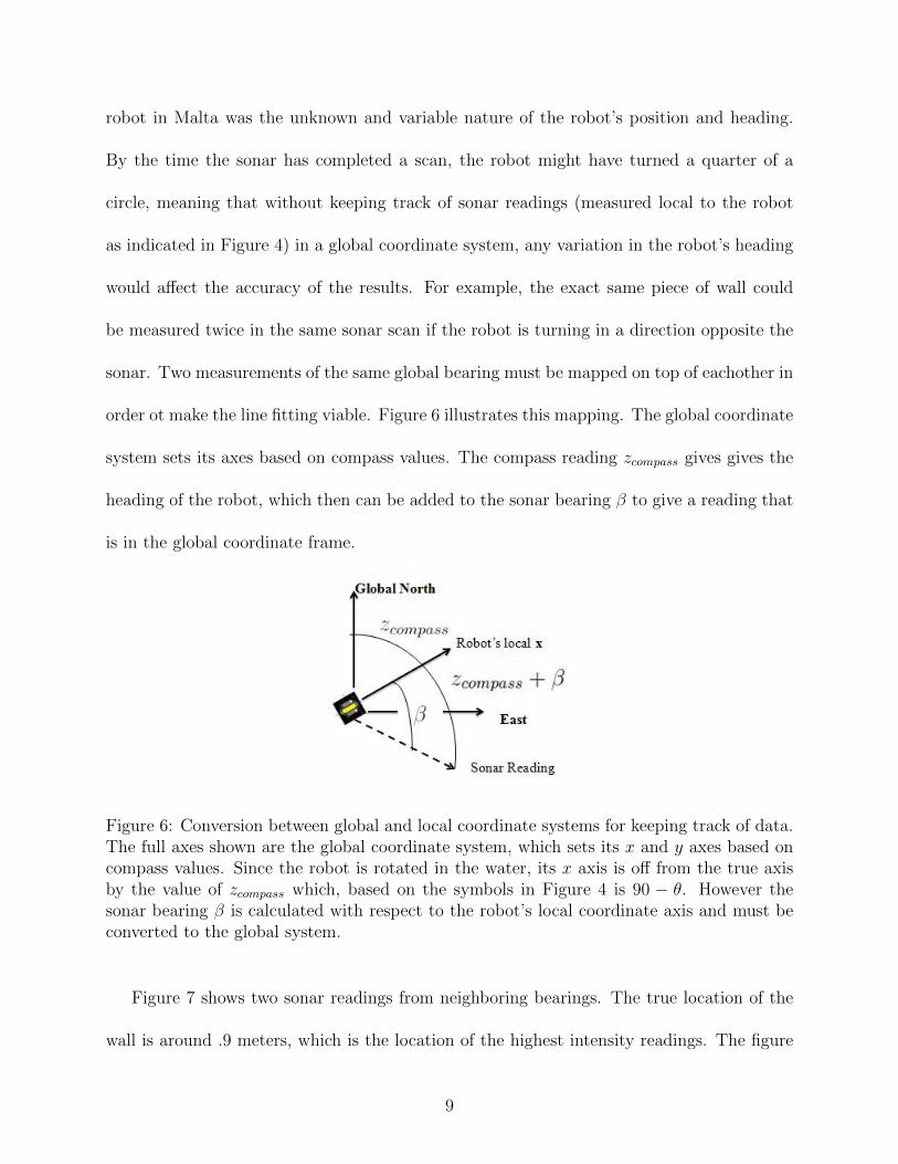
order ot make the line fitting viable. Figure 6 illustrates this mapping. The global coordinate

system sets its axes based on compass values. The compass reading zcompass gives gives the

heading of the robot, which then can be added to the sonar bearing β to give a reading that

is in the global coordinate frame.

Figure 6: Conversion between global and local coordinate systems for keeping track of data.The full axes shown are the global coordinate system, which sets its x and y axes based oncompass values. Since the robot is rotated in the water, its x axis is off from the true axisby the value of zcompass which, based on the symbols in Figure 4 is 90 − θ. However thesonar bearing β is calculated with respect to the robot’s local coordinate axis and must beconverted to the global system.

Figure 7 shows two sonar readings from neighboring bearings. The true location of the

wall is around .9 meters, which is the location of the highest intensity readings. The figure

9

Figure 7: Plot of the sonar intensities at all the distances for two neighboring bearings. Thetrue location of the wall is around .9 meters, which is the location of the highest intensityreadings.

also indicates the various kinds of error that must be dealt with when filtering the distance

of the wall out of the sonar readings.

• There is inconsistency and background noise throughout the data.

• In both sets there is an extra fairly substantial peak very close to 0.0m due to properties

of the sonar. This is present in every reading and does not reflect a true wall.

• There could also be other additional peaks, such as the peak around 1.0m in Bearing1.

This might be because of sound reflecting off multiple smooth surfaces and eventually

returning to the robot. For example, if the sound bounces diagonally off a wall onto

another wall and then back before returning to the robot, the robot will assume that the

first wall is further away than it actually is because of the long time of flight caused

by multiple reflections. Although this is not as large of an issue in the underwater

10

tunnels in the field, when the walls are really smooth such as in a pool, the presence

of multiple reflections can really distort the data.

• In addition, the process of collecting a sonar reading is slow: it takes about 10 seconds

to collect a full circle of readings, so the reading at each bearing β will be refreshed

at best every 10 seconds. Error in sending the data from the sensor might make the

refresh time even longer. If the robot is rotating, the step in the sonar might mean

that particular bearings have a refresh time that is significantly lower than 10 seconds,

although neighboring bearings have been updated.

These kinds of error make efficient filtering for the wall position challenging. Ideally, the

robot would only have to look through the bins once to process the data and accurately

determine the distance to the wall at each bearing.

Additionally, even with perfect processing, there are outliers in the sonar data, where

something in the environment (for example a rock) caused the peak intensity to occur at a

position before the wall. This is why the robot cannot just search for and return the nearest

wall position in the correct quadrant. Instead the processes must be implemented to increase

robustness and reduce error.

2.3 Problem Definiton

The wall filtering algorithm must find (ρβ, αβ) that best represents the distance of the wall

at bearing β. Once all wall points in a window w are found, the wall must be modeled by

fitting a line to those points. The line is represted by ρ, the shortest distance from the robot

to the line, and α, the angle from the robot to this point of shortest distance, so fitting

requires finding parameters ρ, α such that all points (r, θ) on the line satisfy equation 2.

11

r =ρ

cos(θ − α)(2)

After any additional processing to reduce error, the algorithm must output [ρ∗, α∗] that

correspond to the closest line in the correct quadrant for the controller. Figure 8 shows

the individual points (ρβ, αβ) that are fit into a line to produce a [ρ, α], which in this case

ultimately becomes the output [ρ∗, α∗].

Figure 8: Raw wall positions (ρβ, αβ) for each bearing β and line fitting in the global coor-dinate system.

3 Overview of Components

The following sections will outline the individual components of the wall extraction algo-

rithm, which fit together as shown in Figure 9. From the raw sonar measurements zt and

the heading measurement zcompass that are the input to the algorithm, the measurements are

first filtered to give a single wall position for each bearing in the global coordinate system

12

Figure 9: Components of the wall extraction algorithm include finding the wall position(which produces the ρβ, αβ pairs), producing initial windowed line fits with outlier re-moval(the ρ, α pairs), subtractive clustering, and then refitting the lines (producing a singleρc, αc for each cluster) before calculating the output ρ∗, α∗.

where there is information, producing ρβ, αβ pairs for each bearing β, where αβ is just β

converted from the sonar indexing system (which goes from 0 to 6400) into radians. Then

one of two line fitting algorithms are used to fit lines to small windows around each point of

the data, producing ρ, α pairs that describe the line going through each point. These lines

are checked for outliers, and then clustered, and then re-fit to produce a single ρc, αc based

on the larger window of the entire cluster. The nearest ρc, αc in the correct quadrant are

then selected as [ρ∗, α∗].

4 Wall Filtering

As discussed in section 2.1, the sonar produces an array of intensities for every bearing, with

each bin in the array corresponding to a different distance. High intensities indicate the

presence of a wall or other object causing a reflection. The location of the wall is modeled as

13

the cluster of the highest intensity of points. Requiring a cluster (set to size 3 by empirical

investigation with played-back and live data) makes the filtering process more robust against

noise. Algorithm 1 a linear time algorithm for finding this wall cluster by using a moving

threshold. When a cluster of size 3 is found, the threshold is increased to 5 more than the

current maximum value seen. By using the threshold as well as just saving the maximum,

the algorithm ensures that the entire cluster is dealt with easily.

Algorithm 1 [ρβ, αβ] = zt

1: threshold← 50,maxV al← 55, wallCount← 02: for b = 0...numBins do3: if intensity[b] ≥ threshold then4: if intensity[b] > maxV al then5: maxV al← intensity[b]6: end if7: wallCount← wallCount+ 18: else9: wallCount← 0

10: end if11: if wallCount ≥ 3 then12: Save b as current wall candidate13: threshold← maxV al + 514: wallCount← 015: end if16: end for

A few optimizations to the algorithm were necessary based on the constraints of the

hardware. For example, as can be seen in 7, due to properties of the sonar, the scan has a

high peak in some bins close to 0. On scans where there is no wall, this peak near 0 would

get interpreted as a wall. Therefore, bins under .3 meters from the robot are ignored entirely,

and scanning begins after that. Additionally, if no wall is found, the algorithm sets the wall

distance to 9999, which is the indicator value for no data. Since rotation of the robot will

cause any given bearing to have valid data at any time, this ensure that later algorithms

14

such as the clustering algorithm can iterate through the entire range of bearings without

concern of including invalid data.

5 Line Fitting

This project investigated two methods for line fitting. The first method is based on the work

of Siegwart et. al., Nguyen et. al. and Arras and Siegwart who all discuss variations on

a general line fitting algorithm for polar coordinates [13], [8], [1] which they applied to the

general problem of mobile robotics. Essentially, they present least squares error minimization

in the polar space. The second method is a modification of Siegwart’s least squares idea to

just calculate the least squares error in X-Y coordinates. This removes the problem of having

the two measurements be in different units, which can affect the error calculations.

Algorithm 2 [ρ, α] = Line F itting([ρβ, αβ])

Require: 0 ≥ end ≥ maxBearings1: ρ← 9999, α← 99992: w ← [ρiαi] for i = end−WindowSize : end3: [αline, ρline, Rline]← LineFit(w)4: if Rline < TR then5: α← αline6: ρ← ρline7: end if8: Return [ρ, α]

The general outline of both line fitting algorithms is shown in Algorithm 2. First, a

window of a certain number of consecutive readings in the same neighborhood is created.

For any small window w, there is a good chance that all the points (ρβ, αβ) in w are on

the same line. Then, if using Siegwart’s polar method, α and ρ are calculated as shown in

equations 3 and 4 using the equations presented by Siegwart et. al. [13].

15

α =1

2tan−1

( ∑ρ2i sin 2αi − 2

||w||∑∑

ρiρj cosαi sinαj∑ρ2i cos 2αi − 1

||w||∑∑

ρiρj cos(αi + αj)

)(3)

ρ =

∑ρi cos(αi − α)

||w||(4)

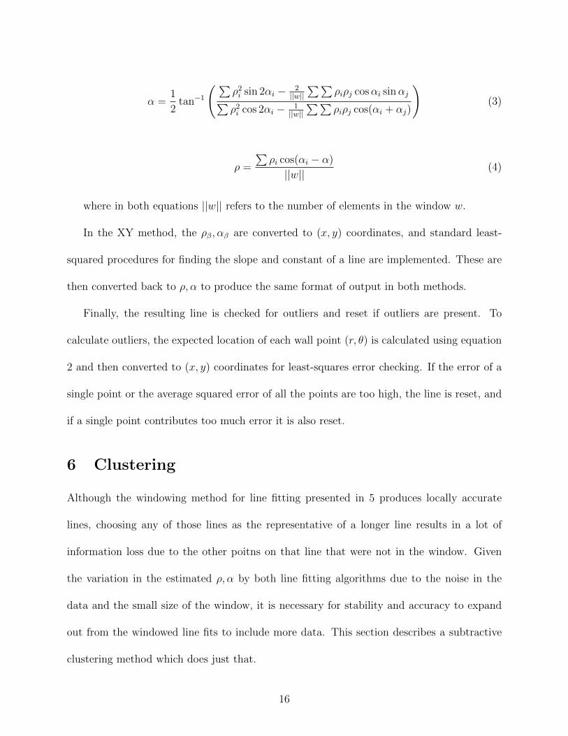
where in both equations ||w|| refers to the number of elements in the window w.

In the XY method, the ρβ, αβ are converted to (x, y) coordinates, and standard least-

squared procedures for finding the slope and constant of a line are implemented. These are

then converted back to ρ, α to produce the same format of output in both methods.

Finally, the resulting line is checked for outliers and reset if outliers are present. To

calculate outliers, the expected location of each wall point (r, θ) is calculated using equation

2 and then converted to (x, y) coordinates for least-squares error checking. If the error of a

single point or the average squared error of all the points are too high, the line is reset, and

if a single point contributes too much error it is also reset.

6 Clustering

Although the windowing method for line fitting presented in 5 produces locally accurate

lines, choosing any of those lines as the representative of a longer line results in a lot of

information loss due to the other poitns on that line that were not in the window. Given

the variation in the estimated ρ, α by both line fitting algorithms due to the noise in the

data and the small size of the window, it is necessary for stability and accuracy to expand

out from the windowed line fits to include more data. This section describes a subtractive

clustering method which does just that.

16

Subtractive clustering was first presented by Chiu [4] [3] to provide a better-performance

alternative to a similar type of clustering algorithm. This implementation adopts Chiu’s

algorithm but changes some of the parameters. Algorithm 3 shows the outline of the sub-

tractive clustering algorithm. Three constant parameters are tunable for different results:

the staring radius, the radius increment and the percentage of the potential that serves as

the cut-off. Chiu [3] suggests a radius increment of 1.25 and a cut-off of .15, while Chen more

recently [2] suggested 1.5 for the increment and .25 for the cut-off. These numbers produced

more accurate experimental results on trial datasets, so the code is currently implemented

using Chnen’s numbers.

The key nuance of Chiu’s algorithm is the calculation of the potential, occuring in this

algorithm on lines . Initially, the potential of each point Pi is set as given by equation 5,

which is essentially a measurement of how many near neighbors each data point has. Then,

on each subsequesnt iteration, each Pi is adjusted by subtracting out a factor related to

its nearness to the previous cluster as shown in equation 6, to avoid having closely spaced

cluster centers.

Pi ←n∑j=1

e−||xi−xj ||

2

(radius2/4) (5)

Pi ← Pi − PrevCenterPotential ∗ e−||xi−xj ||

2

(radius2/4) (6)

17

Algorithm 3 clusters = Cluster([ρ, α])

1: Bound the x and y coordinates produced from data inside a unit hypercube2: radius← .05,maxPotential← 0, clusterNum← 1, currentCenterCandidate← 99993: for i : 0...numBearings do4: Calculate P (xi) using equation 55: if P (xi) > maxPotential then6: maxPotential← P (xi)7: currentCenterCandidate← i8: end if9: end for

10: firstMaxPotential ← maxPotential [note: for use in cutoff later]11: for i : 0...numBearings do12: if ρi, αi is within radius of currentCenterCandidate then13: clustersi = clusterNum14: end if15: end for16: radius← radius ∗ 1.5, clusterNum← clusterNum+ 117: while maxPotential > firstMaxPotential ∗ .25 do18: for i : 0...numBearings do19: Calculate P (xi) using equation 620: if Pi > maxPotential then21: maxPotential← Pi22: currentCenterCandidate← i23: end if24: end for25: for i : 0...numBearings do26: if ρi, αi is within radius of currentCenterCandidate then27: clustersi = clusterNum28: end if29: end for30: radius← radius ∗ 1.5, clusterNum← clusterNum+ 131: end while

18

7 Experiments and Results

The various components outlined in the previous sections were developed iteratively to allow

for greater testing in such a complicated system. In order to run experiments, a significant

amount of logging code was written at each component of Figure 9 to record raw sonar values,

intermediate outputs from each function, and final output values from the wall extraction

algorithm. The code was then run both on saved sonar data from Malta expeditions to

evaluate accuracy and live on the robot, both in Malta and in Princeton’s DeNunzio pool.

Although the pool has different sonar characteristics than a cistern due to its smooth walls

and regular rectangular shape, it did provide a feasible venue for evaluating the performance

of the code after returning from Malta.

Qualitatively, the live tests indicated that the hardware and software interface challenges

had been successfully overcome, with the robot responding to the control signals sent by

the algorithms presented in the paper. Additionally, both live and with the played-back

data there was no indication of lag or slow-down in the code due to the extra processing,

even when the playback speed was the fastest possible or the live data was switched to the

high-speed or high-resolution settings.

For consistency, the rest of the analysis in this section uses a data set recorded in a

cistern under a cathedral sacristine in Mdina, Malta in 20094. The raw sonar scan is shown

in Figure 10a and the result of the wall filtering algorithm is shown in Figure 10b. The

filtering algorithm accurately finds the walls for every bearing where there is a scan and does

so in linear time.

4The sonar log file is Thu 03 Mar 14 27 for anyone seeking to replicate these experiments.

19

(a) The raw sonar scan of one of the2009 Mdina Cathedral Sacristine readings,viewed from the SeaNet Pro software thatacts as the intermediate between sonar dataand the input to the program running therobot.

(b) The result of the wall filtering algo-rithm. The shapes and distances bothmatch the locations of high intensity visi-ble from visual inspection of the raw dataplayback, and except for a few outliers thatresult in the data, give a good foundationfor line fitting.

Figure 10: Raw sonar data and the results of the wall filtering algorithm.

Figure 11 shows the results of the line fitting before outlier removal. In general the output

of the line fitting algorithm is clustered on each line at the location where the perpendicular

emanating from the origin would hit. However, there are a significant number of inaccuate

points near the origin, which are nearly all caused by either the outlier poitns on the left or

(mostly) the data on the right where there is not a smooth line. This indicates the sucess

of the line fitting methods but also the need for outlier removal. Additionally, in Figure 11a

the two line fitting methods (Siegwart et. al. and XY least squares) are compared against

eachother, with Siegwart et. al. in blue and XY least squares in green. The points produced

by the two methods are nearly identical, with all the clusters as well as the inaccurate data in

the middle present in both methods. In fact, many of the selected data points are identical.

This indicates that both methods of line fitting are likely to produce a good result, although

testing with the hardware should verify this.

Finally, Figure 12 shows the results of line-fitting on the clusters produced by the clus-

20

(a) The result of running both line fit algo-rithms on the same scan. The wall distancesproduced by the wall filtering algorithm arein red. The output of the Siegwart et. al.method is in blue and the output of the XYleast squares method is in green.

(b) One wall of the scan, highlighting thetight clustering of points produced by the linefitting algorithm and the accuracy with whichthey are located at the perpendicular to theline of wall distances. The outputs of bothline fitting methods are represented amongthe blue points.

Figure 11: Raw sonar data and the results of the wall filtering algorithm.

tering algorithm instead of just the short windows used for the original line fitting. The

outlier removal, subtractive clustering algorithm, and re-fitting of the lines has caused the

promising but slightly inaccurate line fits (ρ, α) shown in Figure 11 to become the accurate

clustered line fits (ρc, αc) shown in Figure 12, with a single point (ρci , αci) representing each

one of the walls visible in the raw sonar scan.

8 Conclusions and Future Work

The goal for this project was to create model of the walls in an underwater tunnel environ-

ment using noisy sonar readings from an underwater robot, in a reasonably accurate manner

in real time. Based on the framework and experimental results presented above, the wall

extraction algorithms have fulfilled the goal and provided a solution to the problem set out

in section 2. The solution transformed noisy raw sonar data into clustered line estimations

in real time in a way that verifiably matches scans produced in the field. Figure 12 shows

21

Figure 12: The final result of the wall extraction algorithm, right before the single outputis sent back to the controller. The red is still the output of the wall filtering algorithm, andthe blue is the collection of ρc, αc produced after applying the line fitting to the entirety ofthe clusters that resulted from the clustering algorithm.

22

the results of the wall extraction algorithm on the raw sonar data shown in Figure 10a. The

noise has been removed and each wall has been identified with a point (ρc, αc) that represents

its perpendicular. To produce the final output (ρ∗, α∗) shown in the flow chart in Figure 3,

the algorithm would simply select the point (ρci , αci) in the first quadrant that is nearest the

origin.

Future work should focus on additional field experiments to ensure that all parameters

are tuned for optimum accuracy. All of the components of the wall extraction algorithm

rely on fixed parameters: the initial threshold in wall filtering, the window size in the line

fitting algorithms, the criteria that indicate an outlier, and the radii and cut-off points in the

subtractive clustering algorithm. Although some optimization and tuning was done to all of

these, with additional data sets could improve them. This would increase the accuracy and

prevent false clusters formed by outliers. Another interesting area of future work would be

including weights based on distance. Siegwart et. al’s original equations include factors for

the weight of each point, and Chen [2] presents a variation on subtractive clustering that also

incorporates weights. Finally, as is the case with any robotics project, abundant amounts of

testing with the hardware is necessary. The code is set up to integrate with the controller,

but due to lack of time in Malta it has not yet been deployed in a cistern. Hopefully next

year’s Malta team will be able to perform additional field tests with the finished algorithm,

producing more accurate cistern maps than can be achieved with human operators!

23

References

[1] Arras, Kai and Siegwart, Roland. “Feature Extraction and Scene Interpretation forMap-Based Navigation and Map Building” Proceedings of SPIE, Mobile Robotics XII3210, 1997.

[2] Chen et al. “A Weighted Mean Subtractive Clustering Algorithm”. Information Tech-nology Journal 7, (2), 2008, 356-360.

[3] Chiu, Stephen. “Extracting Fuzzy Rules from Data for Function Approximation andPattern Classification”. Fuzzy Information Engineering: A Guided Tour of Applicationsed. Dubois et al. Wiley and Sons, 1997.

[4] Chiu, Stephen. “Method and Software for Extracting Fuzzy Classification Rules bySubtractive Clustering” Fuzzy Information Processing Society, 1996.

[5] Clark et al. “Sites: 2012, 2011, 2009, 2008, 2006”. Malta/Gozo Cistern ExplorationProject. http://users.csc.calpoly.edu/~cmclark/MaltaMapping/sites.html.

[6] Clark et al. “The Malta Cistern Mapping Project: Expedition II”. Procedings of Un-manned Untethered Submersible Technology, 2009.

[7] Hiranandani et al. “Underwater Robots with Sonar and Smart Tether for UndergroundCistern Mapping and Exploration.” Proceedings of Virtual Reality, Archeology and Cul-tural Heritage, 2009.

[8] Nguyen et al. “A Comparison of Line Extraction Algorithms using 2D Laser Rangefinderfor Indoor Mobile Robots.” International Conference on Intelligent Robots and Systems,2005.

[9] Ribas et al. “SLAM using an imaging sonar for partially structured underwater en-vironments.” IEEE/RSJ International Conference on Intelligent Robots and SystemsOctober 2006.

[10] Ribas et al. “Underwater SLAM in a marina environment” IROS 2007. 1455-1460.

[11] Ribas et al. “Underwater SLAM in man-made structure environments” Journal of FieldRobotics 25, 11-12, 2008, 898-921.

[12] Roy et al. “Coastal Navigation: Robot Navigation with Uncertainty in Dynamic Envi-ronments”. Proceedings of International Conference on Robotics and Automation, IEEE,1999, 35-40.

[13] Siegwart et al. Introduction to Autonomous Mobile Robots. Cambridge: MIT Press,2011.

[14] Wang, Wei. “Autonomous Control of a Differential Thrust Micro ROV.” MS Thesis.University of Waterloo, 2006.

24

[15] Wang, Wei and Clark, Christopher. “Autonomous Control of a Differential ThrustROV.” Proceedings of the 2007 International Symposium on Unmanned Untethered Sub-mersible Technology, 2007.

[16] White et al. “The Malta Cistern Mapping Project: Underwater Robot Mapping andLocalization within Ancient Tunnel Systems.” Journal of Field Robotics, 2010.

[17] Wood, Zoe. “Hardware Set Up”. VideoRay ROV Guide. Accessed April 2012. http://users.csc.calpoly.edu/~zwood/teaching/csc572/final11/jwhite09/

AcknowledgementsA very large thank you to my advisor, Professor Chris Clark, for including me on thisproject and guiding me throughout. I learned a lot about research, robotics, developingon a deadline, interfacing between hardware and software and different members of a team,the academic and cultural considerations of doing research internationally, and even how tocontrol a robot by joystick! Thanks also to the rest of the Princeton Malta team: YingxueLi, Andrew Boik, and Austin Walker for being great teammates as we worked to get thehardware and software configured, and also to the Cal Poly team members and our hosts inMalta for giving us a great welcome.

Some equipment for this project was procured with a grant from Princeton School ofEngineering and Applied Science. Thank you!

Honor Code StatementThis paper represents my own independent work in accordance with University regulations.

Anna Kornfeld Simpson, May 8, 2012

25