Autonomous Sensor Path Planning and Control for
Active Information Gathering
by
Wenjie Lu
Department of Mechanical Engineering and Materials ScienceDuke University
Date:Approved:
Silvia Ferrari, Supervisor
Michael Zavlanos
Xiaobai Sun
Jerome Reiter
Dissertation submitted in partial fulfillment of the requirements for the degree ofDoctor of Philosophy in the Department of Mechanical Engineering and Materials
Sciencein the Graduate School of Duke University
2014
Abstract
Autonomous Sensor Path Planning and Control for Active
Information Gathering
by
Wenjie Lu
Department of Mechanical Engineering and Materials ScienceDuke University
Date:Approved:
Silvia Ferrari, Supervisor
Michael Zavlanos
Xiaobai Sun
Jerome Reiter
An abstract of a dissertation submitted in partial fulfillment of the requirements forthe degree of Doctor of Philosophy in the Department of Mechanical Engineering
and Materials Sciencein the Graduate School of Duke University
2014
Copyright c© 2014 by Wenjie LuAll rights reserved except the rights granted by the
Creative Commons Attribution-Noncommercial Licence
Abstract
Sensor path planning and control refer to the problems of determining the trajectory
and feedback control law that best support sensing objectives, such as monitor-
ing, detection, classification, and tracking. Many autonomous systems developed,
for example, to conduct environmental monitoring, search-and-rescue operations,
demining, or surveillance, consist of a mobile vehicle instrumented with a suite of
proprioceptive and exteroceptive sensors characterized by a bounded field-of-view
(FOV) and a performance that is highly dependent on target and environmental
conditions and, thus, on the vehicle position and orientation relative to the target
and the environment. As a result, the sensor performance can be significantly im-
proved by planning the vehicle motion and attitude in concert with the measurement
sequence. This dissertation develops a general and systematic approach for deriving
information-driven path planning and control methods that maximize the expected
utility of the sensor measurements subject to the vehicle kinodynamic constraints.
The approach is used to develop three path planning and control methods: the
information potential method (IP) for integrated path planning and control, the op-
timized coverage planning based on the Dirichlet process-Gaussian process (DP-GP)
expected Kullback-Leibler (KL) divergence, and the optimized visibility planning for
simultaneous target tracking and localization. The IP method is demonstrated on a
benchmark problem, referred to as treasure hunt, in which an active vision sensor is
mounted on a mobile unicycle platform and is deployed to classify stationary targets
iv
characterized by discrete random variables, in an obstacle-populated environment.
In the IP method, an artificial potential function is generated from the expected
conditional mutual information of the targets and is used to design a closed-loop
switched controller. The information potential is also used to construct an infor-
mation roadmap for escaping local minima. Theoretical analysis shows that the
closed-loop robotic system is asymptotically stable and that an escaping path can be
found when the robotic sensor is trapped in a local minimum. Numerical simulation
results show that this method outperforms rapidly-exploring random trees and clas-
sical potential methods. The optimized coverage planning method maximizes the
DP-GP expected KL divergence approximated by Monte Carlo integration in order
to optimize the information value of a vision sensor deployed to track and model
multiple moving targets. The variance of the KL approximation error is proven to
decrease linearly with the inverse of the number of samples. This approach is demon-
strated through a camera-intruder problem, in which the camera pan, tilt, and zoom
variables are controlled to model multiple moving targets with unknown kinematics
by nonparametric DP-GP mixture models. Numerical simulations as well as physical
experiments show that the optimized coverage planning approach outperforms other
applicable algorithms, such as methods based on mutual information, rule-based sys-
tems, and randomized planning. The third approach developed in this dissertation,
referred to as optimized visibility motion planning, uses the output of an extended
Kalman filter (EKF) algorithm to optimize the simultaneous tracking and localiza-
tion performance of a robot equipped with proprioceptive and exteroceptive sensors,
that is deployed to track a moving target in a global positioning system (GPS) denied
environment.
Because active sensors with multiple modes can be modeled as a switched hierar-
chical system, the sensor path planning problem can be viewed as a hybrid optimal
control problem involving both discrete and continuous state and control variables.
v
For example, several authors have shown that a sensor with multiple modalities is a
switched hybrid system that can be modeled by a hierarchical control architecture
with components of mission planning, trajectory planning, and robot control. Then,
the sensor performance can be represented by two Lagrangian functions, one function
of the discrete state and control variables, and one function of the continuous state
and control variables. Because information value functions are typically nonlinear,
this dissertation also presents an adaptive dynamic programming approach for the
model-free control of nonlinear switched systems (hybrid ADP), which is capable of
learning the optimal continuous and discrete controllers online. The hybrid ADP
approach is based on new recursive relationships derived in this dissertation and is
proven to converge to the solution of the hybrid optimal control problem. Simu-
lation results show that the hybrid ADP approach is capable of converging to the
optimal controllers by minimizing the cost-to-go online based on a fully observable
state vector.
vi
Contents
Abstract iv
List of Tables xi
List of Figures xii
List of Abbreviations and Symbols xv
Acknowledgements xxii
1 Introduction 1
2 Problem Formulation and Assumptions 9
2.1 Problem 1: Mobile Sensor Planning for Target Classification . . . . . 13
2.2 Problem 2: Camera Control for Learning Nonlinear Target Kinematics 15
2.3 Problem 3: Mobile Sensor Planning for Target Tracking and Localization 17
3 Information Gain 21
3.1 Information Theoretic Functions . . . . . . . . . . . . . . . . . . . . . 22
3.2 Information Value Functions for Sensor Planning . . . . . . . . . . . 24
4 Motion Planning 31
4.1 Information Cell Decomposition . . . . . . . . . . . . . . . . . . . . . 32
4.2 Information Roadmap Deployment . . . . . . . . . . . . . . . . . . . 34
4.3 Rapidly Exploring Information Random Trees . . . . . . . . . . . . . 36
4.4 Information Potential Approach for Integrated Control and Navigation 38
4.4.1 Information Potential Function . . . . . . . . . . . . . . . . . 39
viii
4.4.2 Switched Controller . . . . . . . . . . . . . . . . . . . . . . . . 42
4.4.3 Information Roadmap for Escaping Local Minima . . . . . . . 44
4.4.4 Propterties of Information Potential Method . . . . . . . . . . 46
4.5 Optimized Coverage Planning . . . . . . . . . . . . . . . . . . . . . . 52
4.5.1 Particle Filter . . . . . . . . . . . . . . . . . . . . . . . . . . . 53
4.5.2 Approximation of DP-GP Expected KL Divergence . . . . . . 55
4.5.3 Strategy for Searching the Optimal Coverage . . . . . . . . . . 62
4.6 Optimized Visibility Motion Planning . . . . . . . . . . . . . . . . . . 63
4.6.1 EKF for Tracking and Localization . . . . . . . . . . . . . . . 65
4.6.2 Robot Motion Planning . . . . . . . . . . . . . . . . . . . . . 67
5 Simulations and Results 72
5.1 Information Potential Approach for Robotic Sensor Classifying Targets 73
5.2 Optimized Coverage Planning for a Camera Monitoring Moving Targets 79
5.3 Optimized Visibility Motion Planning for Robotic Sensor Trackingand Localizing Targets . . . . . . . . . . . . . . . . . . . . . . . . . . 86
6 Hybrid ADP for Switched Systems 90
6.1 Optimal Control Problem of Switched Systems . . . . . . . . . . . . . 91
6.2 Hybrid ADP Approach . . . . . . . . . . . . . . . . . . . . . . . . . . 92
6.3 Hybrid ADP for Optimal Control Problem of Linear Switched Systems 97
6.4 Convergence Analysis . . . . . . . . . . . . . . . . . . . . . . . . . . . 100
7 Conclusions 108
A Algorithms for Optimized Visibility Planning 110
A.1 Robot Controller . . . . . . . . . . . . . . . . . . . . . . . . . . . . . 110
B Algorithms for Hybrid ADP 111
B.1 Hybrid ADP Critic Network Adaptation . . . . . . . . . . . . . . . . 111
ix
B.2 Hybrid ADP Actor Network Adaptation . . . . . . . . . . . . . . . . 112
Bibliography 113
Biography 123
x
List of Tables
5.1 Average efficiency of IP method . . . . . . . . . . . . . . . . . . . . . 78
5.2 Average performance comparison for M “ 27 . . . . . . . . . . . . . 78
xi
List of Figures
2.1 A robotic sensor with vehicle geometry A and sensor FOV A (d “ 2). 11
2.2 Block diagram of autonomous sensor control . . . . . . . . . . . . . . 13
2.3 A robotic sensor with vehicle geometry A and sensor FOV A. . . . . 14
2.4 Illustration of the camera system, where one FOV is zoomed in andthe other is zoomed out. . . . . . . . . . . . . . . . . . . . . . . . . . 16
2.5 FOV of exteroceptive sensor. . . . . . . . . . . . . . . . . . . . . . . 19
4.1 Example of cell decomposition with void (white) and observation (grey)cells and C-obstacles (green) (a), and connectivity graph G (b). . . . 34
4.2 Example of RRIT with milestones, trees, and actual path. . . . . . . 39
4.3 Goal of switched control law for a given inscribed circle with center ξiand a positive constant ε. . . . . . . . . . . . . . . . . . . . . . . . . 43
4.4 Roadmap Construction. . . . . . . . . . . . . . . . . . . . . . . . . . 46
4.5 Inscribed circle for polygon PT i, with center ξi and radius ri. . . . . 47
4.6 Illustration of the changes of the robot FOV due to the translationand rotation of the robot. . . . . . . . . . . . . . . . . . . . . . . . . 68
5.1 Simulation results for two robotic sensors in a workspace with twotargets, two obstacles, and one narrow passage. . . . . . . . . . . . . 75
5.2 Time histories of sensor orientation (a), linear velocity (b), distancefrom C-target (c), and control inputs (d) . . . . . . . . . . . . . . . . 76
5.3 Potential field contour and information roadmap generated to escapelocal minima. . . . . . . . . . . . . . . . . . . . . . . . . . . . . . . . 77
5.4 Details of sensor path obtained by IP method (left) and by classic PFmethod (right) . . . . . . . . . . . . . . . . . . . . . . . . . . . . . . 79
xii
5.5 Examples of target trajectories following the first velocity field; plotsof the velocity vectors on a regular grid. (a) f1, (b) f2, (c) f3, and (d)f4. . . . . . . . . . . . . . . . . . . . . . . . . . . . . . . . . . . . . . 80
5.6 Simulation snapshot . . . . . . . . . . . . . . . . . . . . . . . . . . . 81
5.7 DP-GP expected KL divergence against each possible position of thefuture measurement in the workspace at initial time. Red curves: thetraining trajectories for obtaining MIP; Yellow dots: points of interest. 83
5.8 The mean and variance of the RMS error of thevelocity, ε, obtainedby “DP-GP EKL” (blue, cross line), by “MI” (red, circle line), by“Heuristic” (green, triangle line), and by “Random” (yellow, squareline), given MIP. . . . . . . . . . . . . . . . . . . . . . . . . . . . . . 83
5.9 The percentage of trajectories belonging to the first velocity type ob-served by the sensor during the simulation given MIP. . . . . . . . . 84
5.10 The mean and variance of RMS error of velocity, ε, obtained by “DP-GP EKL” (blue, cross line), by “MI” (red, circle line), by “Heuristic”(green, triangle line), and by “Random” (yellow, square line), givenIIP (left) and LIP (right). . . . . . . . . . . . . . . . . . . . . . . . . 85
5.11 The percentage of trajectories belonging to the first velocity type ob-served by the sensor during the simulation Given IIP (left) and LIP(right). . . . . . . . . . . . . . . . . . . . . . . . . . . . . . . . . . . 85
5.12 An example of the simulation result where the visibility-optimizedapproach enables the robot to keep the target in its FOV at all timeswhile the potential field method loses the target around the 200th timestep, for a FOV with α “ π6 rad and γ “ 2.5 m. . . . . . . . . . . . 88
5.13 Percentage of detections obtained by the proposed optimized visibil-ity and the potential approaches for various opening angles and edgelengths . . . . . . . . . . . . . . . . . . . . . . . . . . . . . . . . . . 89
6.1 Critic and actor network adaptation in hybrid ADP. . . . . . . . . . . 96
6.2 Optimal state trajectory obtained from SDRE solution. . . . . . . . . 99
6.3 Hybrid ADP cost function convergence to optimal solution obtainedby SDRE. . . . . . . . . . . . . . . . . . . . . . . . . . . . . . . . . . 100
6.4 State trajectory optimization for five cycles of the hybrid ADP algo-rithm and convergence to optimal solution obtained by SDRE. . . . . 101
xiii
6.5 Iterations between actor network adaptations and critic network adap-tations. . . . . . . . . . . . . . . . . . . . . . . . . . . . . . . . . . . . 101
xiv
List of Abbreviations and Symbols
Symbols
A Geometry of sensor platform
Ai Geometry of ith sensor platform
B0 Index set of obstacles within the distance of influence
Bi Geometry of ith obstacle, i “ 1, 2, . . . , n
ci Kernel function of the ith velocity field
C Configuration space
Cfree Free configuration space
CB C-obstacle region
χ Mobile agent state
CT C-target region
d0 Influence distance
dlpqq Minimum distance from q in the configuration space
Dpp||qq Kullback-Leibler divergence between p and q
Dαpp||qq α-divergence between p and q
δt Time step
ηjispk ` 1´q Predicted mean of the jisth particle
ei Random variable for environmental conditions of the ith target
E Expectation operator
ε GP RMS
xv
ξpkq Discrete mode
εpkq Measurement history up to time k
ε Largest invariant set, discrete mode set
f Kinematic function
fi ith velocity field
fνpkq System continuous kinematic function given discrete control νpkq
F Set of velocity fields
Dpτq Scaled Euclidian distance along path τ
FA Moving Cartesian frame embedded in A
FAi Moving Cartesian frame embedded in Ai, i “ 1, 2, . . . , r
FW Cartesian frame embedded in W
Hν Hamiltonian given discrete control ν
HpXq Shannon entropy of X
HRαpXq Reny’s entropy of order α
IpX;Y | Zq Conditional mutual information between X and Y given Z
IA Index set of A
IB Index set of B
IT Index set of T
J Objective function
k1 k0 Constant parameter
Kp Constant parameter
lptq Zoom level at time t
L Number of points of interest
Lν Lagrangian given discrete control ν
Λjispk ` 1´q predicted covariance of the jisth particle
L Zoom level set
xvi
λ Gradient of value function with respect to continuous state
M Number of velocity fields
mji Weight for direction sample function
Mk Set of measurements up to time k
Mi Set of measurements on Ti
mpkq Measurement vector
µjpkq Estimated mean of the ith velocity field at time k
N Gaussian distribution
Npjq The index of targets assigned to the jth robotic sensor
M,Nptq Number of agents
Nrpqiq Set of neighbors for ith sensor
NGPR Number of targets correctly classified by GPR measurements
NIR Number of targets correctly classified by IR measurements
NNξλ Critic network
NNξc Actor network
νpkq Discrete control at time k
ω Angular velocity
ωjis Weight of the jisth particle
ppxq Probability density function or probability mass function for ran-dom variable X
π Vector of probability mass
π Policy
φpxq Terminal cost
φ Random variables of interest
ψ Information value function
Pipkq Position measurement history for the ith velocity field up to timek
xvii
Pjipkq Set of particles
qpxq Probability density function or Probability mass function forrandom variable X
q Robot configuration
q0 Robot initial configuration
qi The ith robot configuration
R0 Index set of robots within the distance of influence
T Set of targets T “ tT1, T2, . . . , Tmu
Ti Geometry of ith target, i “ 1, 2, . . . ,m
tf Final time
τ Robotic sensor path
S Geometry of accurate sensor FOV
Si Geometry of the ith sensor FOV, i “ 1, 2, . . . , r
Spqq Set of points in W occupied by S at configuration q
Σjpkq Estimated covariance of the ith velocity field at time k
Trptkq Rapidly-explore random tree at time tk
U Space of admissible control inputs
uptq Configuration of sensor at t
uν Continuous controller given discrete control ν
Upqq Potential function
U jpqq Potential function for the jth robotic sensor
Uattpqq Attractive potential function
U jattpqq Attractive potential function for the jth robotic sensor
U jr pqq Repulsive potential function for the jth robotic sensor by other
robotic sensors
Ureppqq Repulsive potential function
V Value function
xviii
Vi Information value of the ith target
Vipkq Velocity measurement history for the ith velocity field up to timek
V Lyapunov function
Vi Information value ith garget
W Geometry of workspace
W1 Number of targets correctly classified after measurements
W0 Number of targets correctly classified before measurements
wij Probability of the ith target following the jth velocity
x Continuous system state
Xi Random variable for ith cell state, i “ 1, . . . , c
ξi Position vector of qi in the configuration space
X Set of points of interest
X Finite range for X
Xk or Xk Random variable for cell state at time step k
Zi or Zi Measurement at the ith target, i “ 1, . . . , c
zk Measurement at time step k
zk Observation of measurement at time step k
ε Constant number
ε An area with a deterministic size by the user based on the sizeof potential field.
θ Parameter of sensor model distribution, or robotic sensor head-ing angle
θ Random variables representing target characteristics
κi ith cell, i “ 1, 2, . . . , c
Λ Sample space of λk
Λi Random variable for environmental conditions for ith tagret
xix
µ The parameter matrix in the growth curve model
µij The element at ith row jth column of matrix µ
µji Mean for direction sample function
ρgoalpqq The distance between q and the goal
ρbipqq The distance between q and the ith obstacle
ρtipqq The distance between q and the ith target
Abbreviations
ADP Adaptive dynamic programming
BN Bayesian network
BNP Non-parametric Bayesian Model
DP Dirichlet process
DP-GP Dirichlet process Gaussian process
EDG Expected discrimination gain
EER Expected entropy reduction (conditional mutual information)
EKL Expected Kullback-Leibler
FOV Field-of-view
GP Gaussian process
GPR Ground-penetrating radar mounted
IIP Intermediate informative prior
IP Information potential
IRM Information roadmap method
KL Kullback-Leibler
LQ Linear-quadratic
LIP Less informative prior
MCMC Markov Chain Monte Carlo
xx
MI Mutual Information
MIP More informative prior
MPD Motion planning with different constraints
MSP Master-slave procedure
PDF Probability density function
PMF Probability mass function
PRMs Probabilistic roadmap methods
RMS Root mean square
PF Potential field
PSG Player/Stage/Gazebo
RRT Rapidly-exploring random trees
STP Switching table procedure
UAV Unmanned air vehicle
UGV Unmanned ground vehicle
UB Upper bound
xxi
Acknowledgements
First, I would like to thank my advisor, Dr. Silvia Ferrari. Your kindness, help,
support, and dedication to me were invaluable. Your consistent motivation kept
me energized every day, and your academic adventure and experience enhances my
interests in research.
I would also like to give special mention to those faculties who have served their
time and effort: Dr. Michael Zavlanos, Dr. Xiaobai Sun, Dr. Jerry Reiter. In addi-
tion, I would like to thank those who have contributed to my better understanding
of this research: Dr. Rafael Fierro, Dr. Tom Wettergren, Dr. Devendra Garg, Dr.
Krish Chakrabarty. A special thank you to my great labmates and fellow graduate
students, who were always available and willing to help along the way: Guoxian
Zhang, Gianluca Di Muro, Greg Foderaro, Greyson Daugherty, Brian Bernard, Ash-
leigh Swingler, Keith Rudd, Hongchuan Wei, Xu Zhang, Wess Ross, Pingping Zhu,
Vikram Raju, Hersh Tapadia.
I wish to dedicate this dissertation to my family. To my parents, Yongshi and
Xinghua, my sister and brother in law, Wenjuan and Haojun. Thanks for having
provided me a fantastic environment. Your passion and love give me the power and
confidence. To my wife and nushen, Amanda. This will never happen without your
support, understanding, and love.
xxii
1
Introduction
Autonomous sensor control for active information gathering utilizes information the-
oretic functions to assess the value of sensor measurements as a function of sensor
control inputs, random environment variables, and unknown target variables. Sub-
sequently, the expected value of the information function can be optimized with
respect to the sensor mode, the measurement sequence, or the position and orien-
tation of FOV [19, 117, 39, 40, 112]. As a result, the effectiveness of autonomous
sensor systems can be greatly improved in a variety of applications, including mine
hunting [85, 80]; classification and tracking [39, 40]; and the monitoring of urban
environments [28], underwater objects [33], manufacturing plants [22], and endan-
gered species [44]. Furthermore, in many sensor applications, such as monitoring,
maintenance, or surveillance, the set of all measurements that could be acquired
by a sensor significantly exceeds its available power, time, and computational ca-
pabilities [22], such that it is also desirable to minimize distance traveled or energy
consumption. Then, the sensor controller can be designed to account for the FOV
geometry and the robot kinodynamic constraints, such that the sensor configura-
tions that enable the most informative measurements with the minimum energy can
1
be determined [111, 100]. Thus, in this dissertation, the sensor is viewed as an
information-gathering agent that must make decisions on its configuration (position,
orientation, and mode), in order to maximize the sensor performance and minimize
the robot energy consumption.
A key challenge in sensor path planning is to assess the sensor performance that
will result from the sensor decisions before obtaining the future sensor measure-
ments [16, 19, 117]. The sensor performance can be shown to depend on the amount
of information or conversely on the uncertainty associated with a set of unknown
target variables to be inferred from repeated sensor measurements. Thus, the util-
ity of future measurements may be represented by their expected information value
conditioned on the prior measurements and on the environmental variables. Infor-
mation theoretic value functions can be used to quantify the amount of information
associated with the probabilistic model of one or more unknown random variables.
The uncertainty of the random variables can then be minimized by optimizing the
information value functions [101, 51, 52, 86, 93]. Computing information theoretic
functions for one or more random variables in a stochastic process requires knowledge
of their joint probability mass (or density) functions. Because the posterior belief
state in the sensor planning problem is typically unknown, a general approach was
recently presented for estimating the expected information value of the future sensor
measurements, where the expectation is with respect to the future measurements
[23].
In Chapter 3, a systematic approach for estimating information theoretic func-
tions for future sensor measurements is reviewed [111]. Several information value
functions have been proposed in the literature to measure the information value in
sensor planning and management problems. Relative entropy was used to solve a
multisensor-multitarget assignment problem in [82]. The expected discrimination
gain (EDG) derived from the Kullback-Leibler (KL) divergence was used to manage
2
agile sensors with Gaussian models for target detection and classification in [45]. Re-
cently, mutual information for sensor planning was studied in multi-target detection,
classification, and feature inference by ground-penetrating radars and infrared sen-
sors in [16, 112]. In [23], an approach based on mutual information was also presented
for adjusting the configuration of a camera in an object recognition application. In
Chapter 3, the approach taken from [111] is extended to develop a new information
value function for the DP-GP models based on the expected KL divergence. This
new information value function quantifies the expected utility associated with fu-
ture measurements for updating the current DP-GP mixture model and is defined as
the expectation of KL divergence between the current (prior) and posterior DP-GP
models over future measurements given sensor control inputs, in situations where
discretization is not feasible due to high computational complexities. The DP-GP
mixture model provides the necessary flexibility to capture spatial phenomena from
data without overfitting [43].
Because robot motion planning approaches deal with the intersections of dis-
crete geometric objects that are possibly moving, subject to a kinematic or dynamic
equation, many sensor path planning methods are inspired by existing robot mo-
tion planning approaches. Chapter 4 reviews three existing sensor motion planning
approaches originally presented in [15], [113], and [66]: the information cell decompo-
sition approach, the information probability roadmap deploy (IPD), and the rapidly
exploring random information trees (RRIT) approach. However, these existing meth-
ods cannot be implemented in sensor planning when sensor kinodynamic constraints
are considered, the targets are moving and their model is complex, or the proprio-
ceptive and exteroceptive sensor are deployed, respectively. To this end, in Chapter
4, three sensor planning methods are developed, which are the information poten-
tial method (IP) for integrated path planning and control, the optimized coverage
planning based on the DP-GP expected KL divergence, and the optimized visibility
3
planning for simultaneous target tracking and localization. The IP method is demon-
strated on a benchmark problem, referred to as treasure hunt, in which an active
vision sensor is mounted on a mobile unicycle platform and is deployed to classify sta-
tionary targets characterized by discrete random variables, in an obstacle-populated
environment. In the IP method, an artificial potential function is generated from
the expected conditional mutual information of the targets and is used to design a
closed-loop switched controller. The information potential is also used to construct
an information roadmap for escaping local minima. Mutual information is a measure
of the information contained in one random variable about another random variable,
and the information value is represented by a conditional mutual information func-
tion that is developed in [27].
Although many potential navigation functions have been developed for robot mo-
tion planning, they are not applicable to sensor path planning because they do not
take into account the geometries of the targets or sensor FOV, nor do they consider
the target information value [77, 87, 47, 91, 53]. Additionally, the effectiveness of
classical potential field methods is limited by their inability to escape local minima,
their lack of stabilization, and their inability to enter narrow passages [50]. In this
dissertation, a switched control approach based on switched potentials [76] is used
to integrate sensor path planning and control. The resulting switched controller can
be proven to be asymptotically stable and is guaranteed to converge to the target
with the highest information value. Additionally, the same information potential
function is utilized to build a local roadmap for escaping local minima. The nu-
merical simulation results show that the IP controlled robotic sensor is capable of
obtaining measurements from the most valuable targets, entering narrow passages,
and escaping local minima, while avoiding obstacles online. Numerical simulation
results also show that this method outperforms rapidly-exploring random trees and
classical potential methods.
4
The above sensor planning approaches typically assume that a measurement is
obtained if the sensor FOV intersects with the geometry of a stationary target. In
the problem of monitoring moving targets, however, the locations of these targets are
unknown and are estimated by time-varying probability density functions (PDFs).
Therefore, it is difficult to formulate a target with rigid geometry. The next two
approaches are designed to obtain measurements from moving targets. The opti-
mized coverage planning approach maximizes the DP-GP expected KL divergence
(approximated by Monte Carlo integration) in order to obtain optimal sensor control
for learning a DP-GP model. This type of problems is derived from problems that
require learning spatial phenomena, such as a temperature function over a given
workspace, a set of velocity fields, or mappings between two spaces. For exam-
ple, the camera intruder problem requires determining the optimal camera control
to collect informative measurements of targets for estimating unknown target kine-
matics, which are modeled with a DP-GP mixture. The objective is to maximize
the estimation accuracy of the learned target kinematics, i.e., the accuracy of the
DP-GP mixture model. By assuming the camera’s position is fixed and its FOV is
a free-flying object without rotation, the optimized coverage planning is designed
to generate the sensor control by maximizing the DP-GP expected KL divergence
at each time step. The proposed DP-GP expected KL divergence can be approxi-
mated via Monte Carlo integration, and the variance of the KL approximation error
is proven to decrease linearly with the inverse of the number of samples. Numerical
simulations as well as physical experiments show that the optimized coverage plan-
ning approach outperforms other applicable algorithms, such as methods based on
mutual information, rule-based systems, and randomized planning.
The optimized visibility motion planning approach uses an extended Kalman
filter (EKF) to simultaneously track the target and localize the robotic sensor [120,
118, 121]. Within this estimation framework, a controller is derived analytically by
5
assuming the FOV of the exteroceptive sensor can be approximated by a sector with
a fixed orientation and a fixed aperture with respect to the robot. The proposed
optimized visibility approach is applicable to any robot equipped with exteroceptive
sensors, such as a laser scanner or camera, for tracking and localizing moving targets,
and with proprioceptive sensors, such as an odometer, for providing ego-motion
information. The results show that the proposed method is effective at tracking and
localizing a moving target with low target loss rates and outperforms a state-of-the-
art potential method.
Because active sensors with multiple modes can be modeled as a switched hierar-
chical system, the sensor path planning problem can be viewed as a hybrid optimal
control problem involving both discrete and continuous state and control variables.
For example, several authors have shown that a sensor with multiple modalities is a
switched hybrid system that can be modeled by a hierarchical control architecture
with components of mission planning, trajectory planning, and robot control. Then,
the sensor performance can be represented by two Lagrangian functions, one function
of the discrete state and control variables, and one function of the continuous state
and control variables. Because information value functions are typically nonlinear,
this dissertation also presents an adaptive dynamic programming approach for the
model-free control of nonlinear switched systems (hybrid ADP), which is capable of
learning the optimal continuous and discrete controllers online.
A switched hybrid system consists of time-driven and event-driven kinematics.
Event-driven kinematics are described by discrete states and control inputs that are
represented by finite alphabets. Time-driven kinematics (differential or difference
equations) are used to represent systems with continuous states and control in a
Euclidean space. The optimal control of switched systems seeks to determine an op-
timal discrete controller that decides the system mode (event-driven kinematics) and
multiple optimal continuous controllers that regulate the system motion (time-driven
6
kinematics) given the system mode. The discrete and continuous optimal controllers
are determined such that a scalar objective function of the hybrid system states
and control is minimized over a period of time [12]. Switched hybrid systems have
been used to model centralized multi-agent networks in [29, 34] and decentralized
multi-agent networks in pursuit-evasion games in [110]. The optimality conditions
for the optimal control of switched systems are derived in [78] using the Pontryagin
Minimum Principle [79]. A master-slave procedure (MSP) that provides an open-
loop solution for a given initial state and a switching table procedure (STP) based
on dynamic programming were developed in [83] for a switched affine system with a
piecewise quadratic cost function. A parametric-optimization method was proposed
in [109] to optimize the continuous controller and switching time instants for a given
(predesigned) fixed switching sequence. However, these existing approaches cannot
adapt to the uncertainty in system modeling and environment.
Adaptive Dynamic Programming (ADP) is an effective approach for solving non-
linear optimal control problems in the absence of a dynamic model in closed form
that optimizes the performance in the face of unforeseen changes and uncertainties
[31, 73, 75, 84, 59]. In recent decades, ADP has been implemented in a number
of applications involving the optimal control of systems described by continuous
state and control variables [107, 98, 97, 106, 72, 41, 24, 3, 74] or by stochastic sys-
tems characterized by discrete-event state and decisions [99, 7]. ADP has also been
used to determine model-free optimal controllers for zero-sum multi-agent games in
[115, 61, 96, 94] and for affine nonlinear systems in [62, 114]. Despite its successful
implementation and guaranteed convergence [107, 1, 97], the applicability of ADP
to hybrid systems has yet to be fully demonstrated in the literature.
In the remainder of this dissertation, a general hybrid ADP approach is presented
for the model-free control of switched sensor systems, where the optimal continuous
and discrete controllers are determined via online learning. The proposed approach is
7
based on new recursive relationships derived in this dissertation and is proven to con-
verge to the solution of the hybrid optimal control problem. Simulation results show
that the hybrid ADP approach is capable of converging to the optimal controllers by
minimizing the cost-to-go online based on a fully observable state vector.
This dissertation is organized as follows. Chapter 2 presents the autonomous
sensor planning and control problem for active information gathering. The pro-
posed DP-GP expected KL information function is introduced, after a review on
information value functions, in Chapter 3. Three proposed sensor motion planning
approaches are presented in Chapter 4, and the results from the numerical simula-
tions are summarized in Chapter 5. In Chapter 6, the optimal planning problem for
a sensor with multiple modalities is generalized into an optimal control problem of a
switched hybrid system and a proposed hybrid ADP approach is introduced to solve
this problem. Finally, the conclusions are given in Chapter 7.
8
2
Problem Formulation and Assumptions
This dissertation considers the problem of autonomous sensor control for active in-
formation gathering with the objective of decreasing the uncertainty of one or more
random variables. The sensor performance can be greatly enhanced by using control
and data processing methods that consider the sensors, platforms, and their envi-
ronment as an integrated sensor system. The sensor or sensor network is deployed
in a workspace W P Rd, where d is either 2 or 3. The workspace is populated with
M rigid targets that are denoted by T1, . . . , TM , where Ti is a compact subset of W .
The set of targets is represented by an index set IT . Each target Ti, where i P IT , is
characterized by a random state vector θi, which may vary with time. For example,
θi can be used to denote the position and velocity of a target Ti that is moving. Let φ
denote the vector consisting of the random variables whose values are to be inferred
or classified by the sensor. The vector φ is also referred to as the random vector of
interest. The vector could simply be a vector consisting only of θi, i P IT , or it could
be any other unknown vector relating to the targets’ characteristics, measurements,
or environment conditions through a model (e.g., the DP-GP model).
Let a compact set S P Rd denote the geometry of the sensor FOV and FW denote
9
a fixed Cartesian frame with origin OW and embedded in W , and let FS denote a
moving Cartesian frame with origin OS and embedded in S. Assuming S is rigid, the
FOV configuration q “ rx y θsT can be used to specify the position and orientation
of every point in S with respect to FW , where x, y, and θ are the coordinates and
orientation of FS with respect to FW . Let C denote the configuration space and Spqq
denote the subset ofW occupied by S for configuration q; this subset represents the
set of all points in W that can be measured by the sensor when the sensor FOV is
at q. It then follows that the sensor can obtain measurements zi from a target Ti iff
Ti X Spqq ‰ H.
For a mobile robotic sensor, the geometry of its platform is described by a rigid
object, A, that is a compact subset of a workspace W Ă Rd. Assuming A is fixed
with respect to S, let Apqq denote the subset of W occupied by A at configuration
q. Here, A must be considered during planning in order to avoid collisions with any
of the N rigid obstacles, which are denoted by B1, . . . ,BN . An example of a mobile
robotic sensor is shown in Fig. 2.1. The following definitions are then adopted from
[16] and [55] :
Definition 1 (C-target). The target Ti in W maps in the robot’s configuration space
C to the C-target region CT i “ tq P C | Spqq X Ti ‰ ∅u.
Definition 2 (C-obstacle). The obstacle Bi in W maps in the robot’s configuration
space C to the C-obstacle region CBi “ tq P C | Apqq X Bi ‰ ∅u.
The configuration of FOV q is usually controlled by an mechatronical system. For
example, when the sensor is mounted on a mobile platform and fixed with respect
to the platform, the change of the FOV configuration is realized by controlling the
mobile platform, perhaps through the linear acceleration and angular velocity of the
platform. Therefore, the configuration of FOV q must also satisfy certain kinematic
equation imposed by the mechatronical system. This kinematic equation can be
10
FS OS
A
S
FW OW
Figure 2.1: A robotic sensor with vehicle geometry A and sensor FOV A (d “ 2).
described by
9qptq “ fνptqrqptq,uptqs, (2.1)
where uptq is the control input and νptq P E is the discrete mode control. Note that
this kinematic equation can be relaxed when the FOV is modeled as a free-flying
object [55].
The target state θi, the sensor measurement zi, and the sensor parameter/mode
or environmental condition ei are assumed to be continuous random vectors. Then,
the measurement process can be described by a joint PDF that, typically, can be
factorized as
ppθi, zi, eiq “ ppzi | θi, eiqppθiqppeiq, (2.2)
because both θi and ei are independent random vectors. The conditional PDF of
zi given θi and ei is usually referred to as the sensor model. This PDF is obtained
from the physical principles characterizing the measurement process. The PDFs of
θi and ei, known as priors, are computed from available prior environmental infor-
mation. These PDFs are assumed to be uniformly distributed if no prior information
is available. Various sensors have been modeled by (2.2), either from first principles
or from data [32, 17]. A sensor measurement zi is obtained when the sensor FOV
intersects the ith target geometry, i.e., Ti X Spqq ‰ H under condition ei, where ei
is assumed to be known for simplicity.
11
If the unknown vector of interest φ only consists of pθ1, ¨ ¨ ¨ ,θMq and the targets
are independent and time invariant, then the original problem is reduced to inferring
θi for all i in IT . The posterior PDF of θi can be obtained from the measurement
model (2.2) and Bayes’ rule,
ppθi | zi, eiq “ppzi | θi, eiq ppθiq
ş
Θppzi | θi, eiq ppθiqdθi
, (2.3)
for i “ 1, . . . ,M , where Θ is the value space of θi because (2.2) holds for all targets.
In other cases, a statistical model is required to build the relation between φ and
zi for all i in IT . For example, as shown in Chapter 3, the DP-GP mixture model
assumes that φ and zi for all i in IT follow an unknown Gaussian process. The
DP-GP model is used to infer φ and to design an information value function.
The problem considered in this dissertation is to determine the optimal control
for the autonomous sensor such that (I) the uncertainty of φ is minimized, (II) the
energy consumption or distance traveled is minimized, and (III) collisions with all
obstacles are avoided for autonomous sensors with mobile platforms. A block diagram
of this sensor system is summarized in Fig. 2.2. The sensor can be viewed as an
information-gathering agent that must make decisions on its configuration (position,
orientation, and mode), in order to optimize the sensor performance. The sensor
performance prior to obtaining the sensor measurements depends on the amount
of information, or lack thereof, associated with these variables and is quantified by
information value functions. A systematic approach for generating information value
functions is reviewed in Chapter 3. These information value functions are used to
design motion planning approaches in Chapter 4.
Three types of problems that cannot be solved by existing sensor planning meth-
ods are now presented, which will be separately used to demonstrate that the ap-
proaches developed in Chapter 4. In the first problem, the sensor is mounted on a
12
Sensor System
Environment
Measurement Fusion/Estimator
Controller
Output
Figure 2.2: Block diagram of autonomous sensor control
mobile platform and is deployed in a workspace populated with position-fixed tar-
gets and obstacles. This problem is referred to as the treasure hunt problem. The
second problem is referred to as the camera intruder problem. This problem involves
a position-fixed camera monitoring multiple moving targets to learn unknown target
kinematics, where the camera FOV can only cover a portion of the entire workspace
at any given time. This problem assumes that the FOV is a free-flying object. The
third problem involves one mobile robotic sensor with a bounded FOV tracking a
moving target where GPS is unavailable. Thus, the mobile robotic sensor is required
to not only optimally track the moving target but also localize itself.
2.1 Problem 1: Mobile Sensor Planning for Target Classification
This problem considers integrated navigation and control for a robotic sensor to
classify multiple targets in an obstacle-populated environment. The robotic sensor
consists of an unmanned ground vehicle (UGV) equipped with an on-board sensor.
As schematized in Fig. 2.3, the sensor FOV, denoted by S Ă R3, is defined as a
compact subset of W from which the robot can obtain sensor measurements. The
configuration vector q must also satisfy the robot kinematic equation that, in this
13
dissertation, is given by the unicycle model in four-dimensional phase space [57],
9χ “
»
—
—
–
9x9y9θ9v
fi
ffi
ffi
fl
“
»
—
—
–
v cos θv sin θwa
fi
ffi
ffi
fl
“ fpχ,uq (2.4)
where χ P R4 is the robot state, v is the linear velocity, w is the angular velocity,
and a is the linear acceleration. The robot control vector is u “ ru1 u2sT “ ra wsT P
U Ă R2, where U represents the space of admissible control inputs.
FS OS
A
S
FW OW
Figure 2.3: A robotic sensor with vehicle geometry A and sensor FOV A.
The target state θi, the sensor measurement zi, and the sensor parameter/mode
or environmental condition ei are assumed to be discrete random vectors. Note
that, in this problem, the random vector of interest φ in Chapter 2 is given as
φ “ rθT1 , . . . ,θTM s
T . The problem is to plan the path and control for the robotic sensor
in (2.4) such that (I) the uncertainty of φ is minimized, (II) the energy consumption
or distance traveled is minimized, and (III) no collisions with any obstacles occur.
Additionally, in order to reduce the algorithm complexity, it is also assumed that A
is a right prism with the base face adjacent to the xy-plane and that S is a three-
dimensional cone. Obstacles and targets are assumed to be right prisms with their
base faces parallel to the xy-plane. Chapter 4 presents an IP integrated path planning
and control method that achieves (I)-(III) and guarantees asymptotic closed-loop
stability for the robotic sensor.
14
2.2 Problem 2: Camera Control for Learning Nonlinear Target Kine-matics
This problem consists of determining the control input, denoted by u, for a camera
with two possible FOV zoom levels, L “ t1, 2u, to monitor a two-dimensional convex
workspace, W Ă R2. The first zoom level enables the sensor to measure a small
area with high accuracy, and the second zoom level enables the sensor to observe a
larger area with less accuracy. As illustrated in Fig. 2.4, if the position of Os with
respect to Fw is denoted by qptq P W and the FOV is assumed to translate in W
without rotation as a free-flying object, the control vector that fully determines the
configuration of the sensor FOV is uptq “ rqT ptq lptqsT , where lptq P L denotes the
choice of zoom level. The set of points covered by the FOV at time t is denoted by
Sruptqs Ă W . Then, at any time t, the noisy vector measurement of the jth target
position, xjptq PW , and velocity, 9xjptq P R2,
mjptqfi
„
yjptqzjptq
“
„
xjptq ` nx9xjptq ` nv
,nx „ N t0,Σxrlptqsunv „ N t0,Σvrlptqsu
, (2.5)
for j “ 1, . . . ,Mptq, is obtained iff xjptq P Sruptqs, where Mptq is the number of
targets that have entered the workspace up to time t and “„” denotes “is distributed
as”. Velocity measurements are obtained though target position difference in two
consecutive video frames. When xjptq R Sruptqs, the measurement of target j at
t is an empty set, i.e., mjptq “ H. Additionally, it is assumed that data-target
association is perfect. The covariance of noise vector nx (Σx) is assumed to be 0,
and nv is assumed to be normally distributed with zero mean and zero covariance;
thus, the covariance matrix Σv P R2ˆ2 has zero off-diagonal entries. For the two
zoom levels, Σvp1q ă Σvp2q, where ă denotes an element-wise matrix comparison.
An unknown number of targets are allowed to travel through W . Although the
true target states are unknown, it can be assumed that all target behaviors can be
15
Target
Future target trajectory
Sensor FoV,
Fs os Fw q
w S[u(k)]
Sensor
Zoom level one
Zoom level two
Figure 2.4: Illustration of the camera system, where one FOV is zoomed in andthe other is zoomed out.
modeled by a possibly nonlinear time-invariant system,
9xjptq “ firxjptqs, j “ 1, . . . ,Mptq. (2.6)
The vector function fi : R2 Ñ R2, referred to as a velocity field, is also unknown and
is drawn from a set F “ tf1, . . . , fNu of unknown velocity fields to be learned from
data, where N is unknown. For simplicity, it is assumed that Mptq can be determined
without error. Note that there does not exist a one-to-one correspondence between
F and the set of targets. This is because one or more targets inW may be described
by the same velocity field in F , while some velocity fields in F may not describe any
of the targets in W .
The problem is to determine both F and the association between the velocity
fields in F and the targets in W based on the sensor measurements obtained up to
the present time according to the model in (2.5). Let a discrete random variable
gj, with range I “ t1, ¨ ¨ ¨ , Nu denote the index of the velocity field that describes
the behavior of the jth target. The event tgj “ iu represents the association of
target j with velocity field fi P F , as shown in (2.6). It is assumed that gj obeys
an unknown N -dimensional categorical distribution [8] denoted by Catpπq, where
π “ rπ1 . . . πN sT describes the prior probabilities of every possible outcome of gj,
for any j “ 1, . . . ,Mptq, that are assumed independent and identically distributed
16
(i.i.d.) such that
Prtgj “ iu “ πi, @i, j, (2.7)
where Prtgj “ iu is the probability of event tgj “ iu.
Let ξi, i “ 1, . . . , L, denote the L points of interest selected to represent the
velocity field over the workspace. For example, the points can be L evenly spaced
grid points in the workspace. Let X “ rξ1 . . . ξLs be shorthand notation for the
points of interest such that
fipXq “ rfipξ1qT . . . fipξLq
TsT . (2.8)
Then, the random vector of interest is given by
φ fi rf1pXqT . . . fNpXq
TsT . (2.9)
Chapter 3 introduces the DP-GP model connecting φ, the measurements, and the
DP-GP expected KL divergence that is used in the optimized coverage planning
approach in Chapter 4 in order to determing the optimal control, u˚ptq, that enables
the sensors to collect the most valuable measurements for learning tφ,πu.
2.3 Problem 3: Mobile Sensor Planning for Target Tracking and Lo-calization
This problem considers a mobile robotic sensor deployed to track a moving target in
a two-dimensional workspace,W Ă R2. The objective is to obtain a controller for the
robotic sensor such that its ability to track and localize the target is optimized with-
out losing the target, based on proprioceptive and exteroceptive measurements. Let
the target state, position, and velocity be respectively denoted by qt “ rxt yt 9xt 9ytsT ,
xt “ rxt ytsT , and 9xt “ r 9xt 9yts
T . Note that the random vector of interest is given
by φ “ qtpk ` 1q. The target motion in W is assumed to be governed by a lin-
ear stochastic motion model that, in discrete time, can be written as a difference
17
equation,
qtpk ` 1q fi ftrqtpkqs `Gw “ Φtqtpkq `Gw, (2.10)
where w is zero-mean Gaussian white noise with covariance matrix Qt, Φt is the
state transition matrix, and G is the noise Jacobian matrix. Both Φt and G are
assumed to be time-invariant and known a priori.
Let qr “ rxr yr θrsT denote the robot configuration or state with respect to an
inertial (or global) frame of reference FW , and let ur “ rvr ωrsT denote the robot
control vector, where vr is the translational speed and ωr is the angular velocity,
where ur P U and U is the space of admissible control inputs. The kinematics of this
robotic sensor in W can be described by the unicycle motion model [105],
qrpk`1q fi frrqrpkq,urpkq, ks“qrpkq`Brpkqurpkq, (2.11)
where
Brpkq “
»
–
cos θrpkqδt 0sin θrpkqδt 0
0 δt
fi
fl , (2.12)
and δt is the time step size.
The proprioceptive sensor (e.g. odometer) obtains noisy measurements of the
control vector,
zrpkq fi hrrurpkqs “ urpkq ` vrpkq, (2.13)
where vrpkq is white Gaussian noise with a time-invariant and known covariance
matrix Qr, i.e., vrpkq „ N p0,Qrq. The exteroceptive sensor is characterized by a
sector-shaped FOV, denoted by S Ă W , that is rigidly connected to the robot and
has an aperture or central angle α and a range or radius γ, as shown in Fig.2.5. Then,
the motion of any point in S can be described by the robot configuration vector qr,
which includes the robot inertial position xr “ rxr yrsT and heading θr. When the
target is inside the FOV, the exteroceptive sensor can measure its relative distance
18
x
y
α
C
B A
sensor
robot target
xt xr
θt θr
Figure 2.5: FOV of exteroceptive sensor.
and bearing according to the model,
zt fi htpqr,qtq“
$
&
%
rρt θtsT` vt, xt P Spqrq
H, xt R Spqrq(2.14)
where ρt “ xr ´ xt denotes the Euclidean distance between xr and xt, θt is the
angle between the robot heading and the direction from robot to target, and vt is
zero-mean Gaussian noise with covariance Rt.
The workspace W is populated with L stationary landmarks with positions xl “
rx1 y1 . . . xL yLsT that can be used to aid localization. The measurement of the
landmarks also consists of the relative distance and bearing,
zli fi hlpqr,xliq“
$
&
%
rρli θlisT` vl, xli P Spqrq
H, xli R Spqrq(2.15)
for i “ 1, . . . , L, where ρli “ xr ´ xli, θli is the relative angle between the robot
heading and the ith landmark location and vl is zero-mean Gaussian noise with
covariance Rl.
Based on the above robot and target motion model and on the most recent
proprioceptive and exteroceptive measurements, zrpkq, ztpkq, and zlpkq, the goal is
19
to obtain a controller such that its ability to track and localize the target is optimized
without losing the target.
20
3
Information Gain
Information theory addresses the quantification of the amount and the quality of
information, which is accomplished by evaluating the uncertainty of one or more
random variables based on their PMF or PDF and on the environment condition.
Information theoretic functions are a natural choice for representing the information
value because they measure the absolute or relative information content of PMFs
or PDFs. In sensor planning and control problems, the utility of the sensor control
may be represented by the expected information value, where the expectation is with
respect to future sensor measurements. The expected information value can then be
used to estimate the utility of the sensor control prior to obtaining the measure-
ments and therefore be used to determine the sensor control. Because the posterior
belief state in sensor planning is typically unknown, a general approach is reviewed
in this chapter that utilizes information theoretic functions to estimate the expected
information value of a measurement resulting from the sensor control prior to ob-
taining the actual sensor measurements and the posterior belief. The information
theoretic functions are first reviewed in the next section. An approach for deriving
the expected information value functions is subsequently reviewed, followed by its
21
new extension that can be used to derive the expected KL divergence information
function for the DP-GP model.
3.1 Information Theoretic Functions
Information theoretic functions are widely used in many applications to evaluate
the information value of sensor measurements. One such function is the Shannon
entropy, which measures the uncertainty of a discrete random variable θ with a range
Θ. From the PMF ppθq for all θ P Θ, the Shannon entropy is defined as
Hpθq “ ´ÿ
θPΘ
ppθq log ppθq. (3.1)
Similarly, the differential entropy (also referred to as the continuous entropy) extends
the Shannon entropy to PDF and is defined as
Hpθq “ ´
ż
Θ
ppθq log ppθqdθ (3.2)
where θ is a continuous random variable and Θ is the value space of θ.
The Reny information or α-divergence measures the difference (also called dis-
tance) between two PMFs (or PDFs). According to [20], the Reny divergence of
order α for discrete random variables is defined as
Dαpp qq “1
α ´ 1log
ÿ
θPΘ
pαpθq q1´αpθq (3.3)
where p and q are two PMFs of θ. The Reny divergence for a continuous random
variable is obtained by replacing the summation in (3.3) with an integral, as follows:
Dαpp qq “1
α ´ 1log
ż
Θ
pαpθq q1´αpθqdθ. (3.4)
In the sensor motion planning literature, p is the posterior belief of θ given new and
prior measurements, while q is the prior belief of θ given prior measurements. As α
22
converges to 1, (3.3) and (3.4) reduce to the KL divergence, as follows:
DKLpp qq “ÿ
θPθ
ppθq logppθq
qpθq(3.5)
for discrete random variables, and
Dpp qq “
ż
Θ
ppθq logppθq
qpθqdqpθq (3.6)
for continuous random variables, respectively.
As shown in [20], mutual information is a measure of the information content
of one random variable regarding another random variable. The conditional mutual
information of two random variables θ and z, given y, represents the reduction in
uncertainty in θ due to knowledge of z when y is given; it is defined as
Ipθ; z | yq “ Hpθ | yq ´Hpθ | z,yq
“ÿ
Θ
ÿ
Y
ÿ
Zppθ,y, zq log
ppθ, z | Zq
ppθ | yqppz | yq
(3.7)
where Hpθ | yq denotes the conditional entropy of θ given y. Similarly, the condi-
tional mutual information of continuous random variables is obtained by replacing
the summation with a triple integral, as follows:
Ipθ; z | yq “ Hpθ | yq ´Hpθ | z,yq
“
ż
Θ
ż
Y
ż
Zppθ,y, zq log
ppθ, z | yq
ppθ | yqppz | yqdθdzdy
(3.8)
The Cauchy-Schwarz divergence is quite useful when qpθq and ppθq are in non-
parametric forms and is based on the Cauchy-Schwarz (CS) inequality. The Cauchy-
Schwarz divergence is also a measure of the difference between two probability dis-
tributions ppθq and qpθq and is defined for discrete random variables as
DCSpp, qq “ log
ř
θPΘ p2pθq
ř
θPΘ q2pθq
rř
θPΘ ppθqqpθqs2 , (3.9)
23
while for continuous random variables, it is defined as
DCSpp, qq “ log
ş
Θp2pθqdθ
ş
Θq2pθqθ
“ş
Θppθqqpθqdθ
‰2 . (3.10)
The entropy, the α-divergence, the KL divergence, and the Cauchy-Schwarz di-
vergence require knowledge of the posterior ppθq. Therefore, they cannot be used
to compute the expected information value because the posterior PMF is unknown
prior to obtaining the measurements [117]. A general approach for designing infor-
mation value function based on expected information theoretic functions is reviewed
in the next section.
3.2 Information Value Functions for Sensor Planning
As shown in the previous section, computing these information theoretic functions
requires knowledge of the PMFs that represent the prior and posterior belief state
of θ. Although it is assumed that the sensor parameters are known a priori, the
approach can be easily extended to the case in which they must also be controlled.
For simplicity, let the random variables of interest be denoted by φ “ rθT1 ¨ ¨ ¨θTM s
T .
The following derivation assumes that θT1 ¨ ¨ ¨θTM are independent, continuous random
variables. Therefore, without loss of generality, the general approach for deriving the
information value function of a measurement zi with respect to θi proceeds as follows.
If zi is known, the information acquired through zi can be represented by the KL
divergence between the prior belief state, ppθi |Mk´1, eiq, and the posterior belief
state, ppθi | zi,Mk´1, eiq, as
DKLrppθi |Mk´1, zi, eiq ppθi |Mk´1, eiqs, (3.11)
whereMk´1 denotes the accumulated measurement up to time k´1. At time k, the
expected change in belief state brought about by zi can be estimated by taking the
24
expectation with respect to zi. Then, from (3.11), the expected KL divergence can
be represented by
ϕDKLpθi; zi |Mk´1, eiq
” Ezi
DKLrppθi | zi,Mk´1, eiq ppθi |Mk´1, eiqs(
“
ż
ZDKLrppθi | zi,Mk´1, eiq ppθi |Mk´1, eiqsppzi |Mk´1, eiqdzi. (3.12)
The KL divergence can be computed from Mk´1 and the sensor model as follows.
When a measurement zk´1i is obtained from the target Ti at time pk ´ 1q, the
PDF of θi given Mk´1 and ei can be updated using Bayes’ rule,
ppθi |Mk´1, eiq “ ppθi | zk´1,Mk´2, eiq
“ppzk´1 | θi,Mk´2, eiqppθi |Mk´2, eiq
ppzk´1 |Mk´2, eiq
“ppzk´1 | θi, eiqppθi |Mk´2, eiq
ş
Θppzk´1 | θi, eiqppθi |Mk´2, eiqdθi
,
(3.13)
because measurements can be assumed to be conditionally independent given the
target state, i.e.,
ppzk´1 | θi,Mk´2, eiq “ ppzk´1 | θi, eiq. (3.14)
Because ppθi |Mk´2, eiq is known from the previous time step pk´2q and additional
measurements are obtained at subsequent time steps, (3.13) can be implemented
iteratively. Finally, the posterior belief inside the expectation in (3.12) is computed
by applying Bayes’ rule for every possible value of zi as follows:
ppθi | zi,Mk´1, eiq “ppzi | θi, eiqppθi |Mk´2, eiq
ş
Θppzj | θi, eiqppθi |Mk´2, eiqdθi
. (3.15)
Similarly, the expected α-divergence can be obtained by replacing the KL diver-
25
gence with the α divergence as follows:
ϕDαpθi; zi |Mk´1, eiq
” Ezi
Dαrppθi | zi,Mk´1, eiq ppθi |Mk´1, eiqs(
“
ż
ZDαrppθi | zi,Mk´1, eiq ppθi |Mk´1, eiqsppzi |Mk´1, eiqdzi (3.16)
where ppθi | zi,Mk´1, eiq and ppzi |Mk´1, eiq can be obtained from (3.13) and (3.15).
The conditional mutual information consists of an expectation of the unknown
measurement in nature and is used to represent the reduction in the uncertainty of
θi caused by zi, which is given by
ϕIpθi; zi |Mk´1, eiq ” Ezi
Ipθi; zi |Mk´1, eiq(
“ Hpθi |Mk´1, eiq ´ Ezi
Hpθi | zi,Mk´1, eiq(
“ Hpθi |Mk´1, eiq ´
ż
zj
Hpθi | zi,Mk´1, eiqppzi |Mk´1, eiqdzi
(3.17)
where the entropyHpθi | zi,Mk´1, eiq is computed from (3.15). The expected Cauchy-
Schwartz information function is defined as
ϕCSpθi; zi |Mk´1, eiq ” Ezi
DCSrppθi | zi,Mk´1, eiq, ppθi |Mk´1, eiqs(
“
ż
Zlog
ş
Θp2pθi | zi,Mk´1, eiqdθ
ş
Θp2pθi |Mk´1, eiqdθ
“ş
Θppθi | zi,Mk´1, eiqpθqppθi |Mk´1, eiqdθ
‰2 dzi,
(3.18)
and it can be used to obtain an alternative measure of the distance between the prior
and the posterior belief states.
As shown in [103], the expected KL divergence can be specialized to the DP-GP
expected KL divergence, where the random vector of interest φ does not consist of
θi. Instead, φ is a vector of other random variables defined as follows:
φ fi rf1pXqT . . . fNpXq
TsT , (3.19)
26
where fi is an unknown velocity field function. The DP-GP model is used to connect
φ and the measurements that are denoted by mpkq.
The DP-GP mixture model for describing target behaviors is studied in [43].
Based on the model of the targets’ kinematics (2.6), every velocity field, fi, projects
the jth target position, xjpkq, to the target velocity, vjpkq, and it can thus be viewed
as a two-dimensional spatial phenomenon, which can be modeled by multiple-output
Gaussian processes (GPs) [38]. Then, a PMF π describing the prior probability of an
association between a target and a velocity field (GP) is learned from data to cluster
the velocity fields using Dirichlet processes (DPs) [9]. DPs can be successfully applied
to data clustering without specifying the number of clusters a priori because they
allow the creation and deletion of clusters when necessary as new data is obtained
over time. The DP-GP mixture model taken from [43] is given as follows:
tθi,πu „ DPpα,GP0q, i “ 1, . . . ,8
Gj „ Catpπq, j “ 1, . . . ,M
fGjpxq „ GPpθGj , cq, @x PW , j “ 1, . . . ,M,
(3.20)
where the strength parameter is denoted by α [92]. For a rigorous definition and a
comprehensive review of DPs, the reader is referred to [25]. In this dissertation, the
base distribution is chosen to be a Gaussian process, GP0 “ GPp0, cq. Let a Gaussian
process GPi represent the distribution of velocities over the workspace specified by
the ith velocity field, fi, such that
fipxq „ GPi, @x PW , (3.21)
for i “ 1, . . . , N . The Gaussian process, GPi, is completely specified by its mean
function θi : R2 Ñ R2,
θipxq “ Erfipxqs, @x PW , (3.22)
27
and its covariance function,
cipxı,xq “ E
rfipxıq ´ θipxıqsrfipxq ´ θipxqsT(
fi
„
cxxpxı,xq cxypxı,xqcyxpxı,xq cyypxı,xq
(3.23)
for all xı,x PW .
Similar to the approach for deriving the information function previously intro-
duced, the proposed DP-GP expected KL divergence is the expectation of the utility
of mjpk ` 1q for updating the current DP-GP model. In this case, the future mea-
surement mjpk` 1q and the association between the target and the velocity field are
unknown. Let Epkq denote the measurement histories of all of the targets already
used for updating the DP-GP model, and let Eipkq denote the measurement history
assigned to the ith velocity field by the DP-GP mixture model.
Then, following (3.16), the DP-GP expected KL divergence for a future measure-
ment mjpk ` 1q can be defined as
ϕjrφ; mjpk ` 1qs “
Nÿ
i“1
wijEmjpk`1qDKL
!
prfipXq|mjpk 1q,Mjpkq, Eipkqs prfipXq|Mjpkq, Eipkqs)
(3.24)
where wij is the probability of the target j following fi and Mjpkq denotes the
measurements from target j up to time k.
The DP-GP expected KL divergence (3.24) requires wij and a PDF of mjpk` 1q
that is a function of xjpk ` 1q and yjpk ` 1q, which are also unknown. The PDF
of mjpk ` 1q is obtained as follows. When Gj “ i and xjpk ` 1q P Srupk ` 1qs, the
estimated measurement distribution is obtained by marginalizing the measurement
model over the estimated target position distribution such that
prmjpk ` 1q|Mjpkq, Eipkqs “ż
Xprmjpk ` 1q|Mjpkq, Eipk,xjpk ` 1qs
ˆ prxjpk ` 1q|Mjpkq, Eipkqsdxjpk ` 1q (3.25)
28
where prxjpk ` 1q|Mjpkq, Eipkq,upkqs is obtained from the current DP-GP model
and the current target position estimation as follows. Recalling (2.6), the target
kinematics can be integrated using the Euler method for a time interval δt such that
xjpk ` 1q “ xjpkq ` vjpkqδt (3.26)
where vjpkq is from the current DP-GP model given xjpkq. Therefore, the estimated
target position distribution at k ` 1 is obtained by the following integral:
prxjpk ` 1q|Mjpkq, Eipkqs “ż
VfXrxjpk ` 1q ´ vjpkqδtsfV rvjpkq,xjpkqsdvj (3.27)
where fX and fV represent the probability density functions of the target position
and velocity at time step k, respectively:
fXrxjpkqs fi prxjpkq|Mjpkq, Eipkqs, (3.28)
fV rvjpkq,xjpkqs fi N rvjpkq;µjpkq,Σjpkqs, (3.29)
where the mean and variance of the jth target velocity at position xjpkq are given
by
µjpkq “ θipxjpkqq `Cpxjpkq,PipkqqrCpPipkq,Pipkqq ` σ2vIs
´1rVipkq ´ θipPipkqqs,
(3.30)
and
Σjpkq “ crxjpkq,xjpkqs ´Crxjpkq,PipkqsrCpPipkq,Pipkqq ` σ2vIs
´1CrPipkq,xjpkqs.
(3.31)
Here, the matrices of the position and velocity measurements in Eipkq are defined as
Pipkq fi ry1p1q . . . yjp`q . . . yMpkqs, @ryTj p`q zTj p`qsTP Eipkq, (3.32)
and
Vipkq fi rz1p1q . . . zjp`q . . . zMpkqs, @ryTj p`q zTj p`qsTP Eipkq. (3.33)
29
The probability of target j following velocity field i can be inferred from Bayes’
theorem,
wij fi prGj “ i|Mjpkq, Epkqs “prMjpkq|EipkqsprGj “ i|Epkqs
řMi“1 prMjpkq|EipkqsprGj “ i|Epkqs
(3.34)
where the prior PMF of Gj given Epkq and upkq is the categorical distribution of
the current DP-GP model. Taken from [43], the likelihood prMjpkq|Eipkq,upkqs is
obtained from the ith GP (velocity field) of the current DP-GP model:
prMjpkq|Eipkqs “kź
`“k1
N rzjp`q; µjp`q, Σjp`qs, (3.35)
where the estimated mean, µjp`q, and covariance, Σjp`q, are calculated by replacing
xjpkq with yjp`q in both (3.30) and (3.31). When xjpk ` 1q R Srupk ` 1qs, no
measurement is obtained and the prior and posterior DP-GP models are the same;
in this case, the DP-GP expected KL divergence (3.24) is zero.
From the above analysis, with the given probability models of mjpk ` 1q, (3.24)
becomes
ϕjrφ; mjpk ` 1qs
“
Nÿ
i“1
wij
ż
Srupk`1qs
ż
Z
D tprfipXq|Mjpk ` 1q, Eipkqs prfipXq|Mjpkq, Eipkqsu
ˆN rzjpk ` 1q;µjpk ` 1q,Σvsdzjpk ` 1q
ˆ prxjpk ` 1q|Mjpkq, Eipkqsdxjpk ` 1q. (3.36)
The calculation of (3.36) involves a 6th-order integral (including an implicit double
integral in D) that is reduced to a double integral in Chapter 4 with proper assump-
tions. Then, the optimized coverage approach is used to maximize the proposed
DP-GP expected KL divergence information function to obtain the optimal sensor
control for the camera intruder problem.
30
4
Motion Planning
In many applications, the sensors are mounted on platforms that consist of au-
tonomous mobile robots or mechatronic structures whose kinematics can be mod-
eled by differential equations. To optimize the sensor performance, the sensor motion
planning and control must consider the stochastic measurement process and filters
for estimation, classification, and prediction. Additionally, sensor motion planning
must take into account the geometry of the sensor’s platform and FOV as well as the
geometry and location of targets and obstacles to determine a path that optimizes
the sensing objectives while avoiding collisions with obstacles and other sensors.
Because robot motion planning approaches deal with the intersections of dis-
crete geometric objects that are possibly moving, subject to a kinematic or dynamic
equation, many sensor path planning methods are inspired by existing robot mo-
tion planning approaches. Chapter 4 reviews three existing sensor motion planning
approaches originally presented in [15], [113], and [66]: the information cell decompo-
sition approach, the information probability roadmap deploy (IPD), and the rapidly
exploring random information trees (RRIT) approach. However, these existing meth-
ods cannot solve sensor planning problems when sensor kinodynamic constraints are
31
considered, the target model is complex, or the proprioceptive and exteroceptive
sensor are deployed, respectively. The IP approach is presented for generating a
potential navigation function and roadmap based on a probabilistic model of the
measurement process and on the geometries of targets and sensor FOV [68]. The
above approaches assume that a measurement is obtained once the sensor FOV in-
tersects with the geometry of the stationary target. For the problem of monitoring
moving targets, the locations of these targets are unknown and are estimated by
time-varying probability distributions. Therefore, it is difficult to formulate a target
with a rigid geometry. To this end, two sensor motion planning approaches are de-
veloped for problems where positions of mobile targets are unknown: the optimized
coverage planning based on the DP-GP expected KL divergence and the optimized
visibility planning for simultaneous target tracking and localization.
4.1 Information Cell Decomposition
Cell decomposition is a well-known approach for decomposing the obstacle-free robot
configuration space into a finite collection of non-overlapping convex polygons that
are referred to as cells, with the purpose of obtaining a robot path without collisions
with obstacles. In classical cell decomposition, the union of these non-overlapping
cells is equivalent to the free configuration space through a line-sweeping algorithm.
Then, a connectivity graph is constructed based on these cells by adding an arc
between two cells if the two cells are adjacent. The connectivity graph can then be
searched for the shortest path between the two cells containing the desired initial and
final robot configurations. One advantage of cell decomposition is that it guarantees
collision avoidance between a robot with any discrete geometry and obstacles of any
shape that are not necessarily convex. One commonly used decomposition method
is known as approximate-and-decompose [119].
The cell decomposition approach for sensor motion planning was proposed in
32
[16]; it modifies the classical cell decomposition approach by taking into account the
presence of the targets and the sensors’ FOV. This approach maps the information
values of position-fixed targets into the cells formed by decomposing the free configu-
ration space, with the goal of classifying the targets located in an obstacle-populated
workspace. Then, similar to the classical cell decomposition approach, a connectivity
graph is built to represent the connectivity relationship between cells and is further
transformed into a decision tree from which an optimal sensor path can be found.
Contrary to classical cell decomposition approaches, the free configuration space
is decomposed into two types of cells. The first type, called an observation cell, is
a convex polygon Dz and a sensor at any configuration in this observation cell can
make an observation of at least one target. In other words, the information value
of an observation cell is positive. The remaining cells are referred to as void cells
that have zero information values, meaning that a sensor at any configuration in a
void cell cannot take measurements of any target. The cell decomposition approach
for sensor planning consists of three steps. The first step is to generate a convex
polygonal decomposition, Dvoid, of the configuration space that is not covered by
any C-obstacles or C-targets. Then, the second step generates a convex polygonal
decomposition, Di, of each obstacle-free C-target, constructing Dz. In the last step,
a connectivity graph G using all cells in D “ DvoidYDz is constructed. Note that the
presence of obstacles and targets makes the decomposition in the first step NP-hard
[60]. The cells containing the initial configuration q0 and the final configuration qf
are referred to as the initial cell (m0) and final cell (mf ), respectively. Examples of
the polygonal decomposition and connectivity graph are illustrated in Fig. 4.1.
As shown in [2], the A˚ algorithm is the most effective in searching for the path
of minimum total distance in G. The A˚ algorithm explores G iteratively, starting
at m0 and visiting every neighbor node mi, where a cost function is assigned by
estimating the minimum-cost path from m0 to mf , through mi. After a node in G
33
m0
m2 m6
m1
m3
m5
7
m11
m9 m4
m8
m10
m0
m2 m6
m1
m3 m5
m7 m11
mf
m9 m4
m8
m10
1
2 2
2 1
1
2
2
3
2 1
3
3 2 2
4 2
(a) (b)
mf
m7
Figure 4.1: Example of cell decomposition with void (white) and observation (grey)cells and C-obstacles (green) (a), and connectivity graph G (b).
is visited, the algorithm stores only the path of minimum cost and labels the node
as visited, assigning it a pointer to its parent node. This process forms a spanning
tree of the subset of G that has already been explored and produces considerable
computational savings compared to other graph-searching algorithms [55, 80].
4.2 Information Roadmap Deployment
Probability Roadmap Method (PRM) algorithms have been shown to be very effec-
tive at planning collision-free paths for robots with many degrees of freedom [90, 11].
The PRM method samples milestones from the free configuration space and con-
structs a roadmap graph. Then, a collision-free path from the initial configuration
to the final configuration is determined from the roadmap by searching the resultant
roadmap graph [46]. An information value-based probabilistic roadmap method,
referred to as the Information Probability Roadmap Deploy (IRD) approach, was
proposed in [112]. The IRD approach samples a roadmap using a hybrid sampling
method for a robotic sensor deployed to classify multiple position-fixed targets in a
workspace populated with obstacles. The hybrid sampling method consists of a PDF
constructed from an information theoretic function that favors samples with a high
expected value of information, a Gaussian distribution covering narrow passages, and
34
a uniform distribution covering wide-open regions.
The information value of the measurements that can be obtained from a robotic
sensor at configuration q is the cumulative information values of these C-targets,
denoted by V pqq. Then, the sampling PDF based on the information value function
is given by
pV pqq “V pqq
ş
CT V pqqdq. (4.1)
It can be shown that this PDF favors milestones with higher information values.
The above PDF is used together with a uniform PDF pUpqq and a Gaussian PDF
pGpqq to form a hybrid sampling approach. The probability of using pV , pU , and
pG to sample a given milestone is v1, v2, and 1 ´ v1 ´ v2, respectively. The IRD
approach first samples one index from t1, 2, 3u with categorical probabilities v1, v2,
and 1 ´ v1 ´ v2, then the corresponding distribution is used to sample a milestone
mi. This sampling process iterates L times to create the nodes of the roadmap
G “ pM,Eq. Subsequently, the set of arcs E is obtained by a local planner that
connects every milestone mi P M with its k nearest milestones. The arc from mi
to its neighbor mj is associated with a traveling distance W rmi`1 ´mis, where
¨ represents the Euclidian norm [88]. The constant parameter k is a user-defined
parameter that is chosen based on Nm and on the complexity of W .
Let τ denote a trajectory; then, the total path distance is given by the sum of all
weighted Euclidian norms along a path τ :
Dpτq “f´1ÿ
i“0
W rqpiq ´ qpi` 1qs, (4.2)
where qpiq is the robot configuration at i along τ . The total reward is defined as
V pτq “f´1ÿ
i“0
V rqpiqs. (4.3)
35
Because the goal of the robotic sensor is to maximize the measurement information
profit and minimize the traveling distance, after connecting the initial configuration
and final configuration in G, the objective function to be maximized is given by
Rpτq “ wV V pτq ´ wD Dpτq (4.4)
where the user-defined constants wV and wD weigh the trade-off between V pτq and
Dpτq. As shown in [2], the A˚ algorithm is the most effective algorithm in searching
for the path of minimum total distance in G.
4.3 Rapidly Exploring Information Random Trees
Rapidly-Exploring Random Trees (RRTs) provide an efficient way to search for a path
in a configuration space online and have been successfully applied to nonholonomic
robots in high-dimensional workspaces. Using the initial robot configuration, the
tree is expanded by iterating incrementally over the discrete time index tk “ 1, 2, . . .
as follows. First a configuration q is randomly sampled from the free configuration
space using a PDF ppqq, possibly uniform or Gaussian. Then, based on a distance
metric, the closest node to q in the tree is computed and extended toward q within a
predefined distance ε to obtain q1. If the path lies in the free configuration space, q1
and this path are added to the tree; otherwise, they are discarded and a new random
configuration is re-sampled.
The modified RRT method with a new sampling method is presented for sensor
path planning [66], where the PDF ppqq is generated based on the geometry and
information value of the target using a normal mixture. The sampled configura-
tions are ordered based on the robotic sensor state (exploration or exploitation), the
expected information value of the target assigned to the sensor, and the distance
to the target. The RRTs are expanded by verifing the feasibility of these sampled
configurations and connecting feasible milestones to the current trees.
36
Let Θi “ pθ1i , θ
2i , . . . , θ
ni q P R denote the directions of all the rays emitted from
the center of FAi, and let µji denote the orientation of θji in FA. Let Lipqq “
pl1i , l2i , . . . , l
ni q P < denote the magnitude for each ray. Assume the distribution of θsi
is a mixture of normal distributions with n components. Each normal distribution
corresponds to an orientation of the vector of the 2-dimensional FOV. Then, for the
ith robotic sensor, the direction of the sth ray is given by
θsi „nÿ
j“1
mjiNpµ
ji , σ
21iq (4.5)
where mji is the weight for the jth normal distribution, µji is the mean and is set
to the direction of the jth reflex, and σ1i is the standard deviation. Similarly, the
magnitudes of Lipqq can also be sampled.
Once a number of milestones are sampled for the ith sensor, they are ordered
based on their importance (or priorities). When the robotic sensor is in the explo-
ration state, the importance of a milestone is proportional to the distance between
the sample and the robot’s current state, given by
Rpqq “ ρipqq (4.6)
where ρipqq is the distance between q and the agent. From the above definition, the
robotic sensor favors a milestone that is far away from its current configuration. For
the robotic sensor in the exploitation state (i.e., the priority is to make a measurement
from a nearby target), the importance is defined as
Rpqq “ k2e´ 1
2fρipqq2` k1
ÿ
jPNi
e´
ρjpqq2
2eV pjq2 (4.7)
where k1 and k2 are two constant representing the weight, Ni is the index of targets
that is assigned to the ith robotic sensor, ρjpqq is the distance between q and the
jth target, and V pjq is the information value of the jth target. Thus, the sampler
37
prefers to generate a sample with a large distance from its current configuration and
a small distance from its assigned targets.
During online sensor path planning, a global RRIT does not exist and is not
necessary for each robotic sensor. A local RRIT is constructed and updated for
each robotic sensor during its movement. Because the robotic sensor always moves
towards sub-root of the subtree expanded to the milestone with highest value of R,
it is not necessary to keep other sibling trees. The tree of milestones is updated
when the robotic sensor reaches the root of the tree. The tree is updated online by
iterating between the following three steps. In the first step, a number of milestones
(configurations) are sampled and are sorted in descended order of their importance
values. Then, the feasibility of the sampled milestone is checked by computing the
expected path to the selected milestone q from the nearest milestone (measured
with the Euclidian distance) stored at the nodes of the tree. In other words, this
step verifies that the entire expected path lies in the free configuration space. During
the last step, the feasible node of the highest importance value is chosen as the goal
configuration. Then, the robotic sensor navigates to this node by the controller used
to check the path feasibility. One example is shown in Fig. 4.2.
4.4 Information Potential Approach for Integrated Control and Nav-igation
This section presents an approach for building a potential navigation function and
roadmap based on the information value and geometry of the targets, referred to
as the information potential (IP) method. A novel information potential function
is introduced, followed by a switched feedback controller for integrated sensor path
planning and control and an information roadmap algorithm for escaping local min-
ima.
38
Tree Expansion Example
T2
T1
B2
B1
W
A1S1
T3
D1
Figure 4.2: Example of RRIT with milestones, trees, and actual path.
4.4.1 Information Potential Function
Because the number of targets correctly classified by a sensor cannot be established a
priori, objective (I) is achieved by maximizing the expected information value of the
measurements, defined as the reduction of uncertainty in the target state θi brought
about by zi. As shown in Chapter 3, prior to obtaining a noisy measurement value
zi, the expected information value of target Ti can be measured by the expected
conditional mutual information,
Vi fi EzitIpθi; zi | eiqu “ Hpθi | eiq ´ Ezi tHpθi | zi, eiqu
“ Hpθiq ´ÿ
zi
ppzi | eiqHpθi | zi, eiq(4.8)
where Hpθi | eiq “ Hpθiq because xi and ei are independent. This information value
is mapped onto the C-target to construct a potential field.
Similar to classical potential approaches, the robotic sensor’s potential function
is the sum of the attractive and repulsive potentials,
Upqq “ Uattpqq ` Ureppqq, (4.9)
39
where the total attractive potential is obtained by multiplying attractive potentials
from all targets together, given by
Uattpqq fiMź
i“1
U itrgpqq. (4.10)
In the proposed IP approach, the attractive potential is obtained by mapping the
information value of a target onto the C-target region of this target in W , given by
U itrgpqq fi η1σV
bi
"
1´ exp
„
´ρipqq
2
2σV bi
*
, i “ 1, . . . ,M (4.11)
where ρipqq denotes the minimum Euclidian distance between q and Ti in C. The
constant η1 is positive, representing the importance of targets relative to other path
planning objectives, such as avoiding collisions with obstacles. The influence distance
of the target is determined by σ and b that are two positive constants. It can be
shown that every C-target in C is a local minimum.
The total repulsive potential consists of two different repulsive potentials that are
defined for fixed and moving obstacles and is given by
Ureppqq fiÿ
lPB0
U lobspqq `
ÿ
jPR0
U jrobpqq, (4.12)
where sets B0 and R0 are the index sets of the considered obstacles and robots.
For fixed obstacles, a potential barrier is generated around the C-obstacle region to
prevent collisions and, at the same time, to allow the robot to obtain measurements
from nearby targets. For a fixed obstacle Bl Ă W , the C-obstacle CBl “ tq P
C | ApqqXBl ‰ ∅u is computed and used to determine the minimum distance from
q in the configuration space:
%lpqq “ minq1PCBl
q´ q1. (4.13)
40
Let B denote the index set of fixed obstacles detected in W up to the present time.
Then, the repulsive potential for Bl, l P B, is
U lobspqq fi
$
&
%
12η2
´
1%lpqq
´ 1d0
¯2
Uattpqq if %lpqq ď d0
0 if %lpqq ą d0(4.14)
where η2 is a positive scaling factor that represents the importance of fixed obstacles
relative to other path-planning objectives and d0 is the obstacle distance of influence
[55].
The repulsive potential of a moving obstacle creates a virtual barrier in C re-
gardless of the presence of targets within the distance of influence. Let R denote
the index set of moving obstacles detected in W up to the present time. Then, the
repulsive potential for Bj with j P R is
U jrobpqq fi
$
&
%
12η3
´
1%jpqq
´ 1d0
¯2
if %jpqq ď d0
0 if %jpqq ą d0(4.15)
where η3 is a positive scaling factor that represents the importance of moving obsta-
cles relative to other path-planning objectives.
As in classical potential field methods [55], a virtual force proportional to the
negative gradient of the potential function (4.9) is used to control the robotic sensor
and is comprised of the sum of an attractive and a repulsive force, generated by
the corresponding potentials. The gradient of the potential function (4.9) can be
obtained as follows:
∇Upqq “ ∇Uattpqq `∇Ureppqq
“ÿ
lPB0
Flpqqvlpqq `Mÿ
i“1
rNipqq ` Aipqqsnipqq ´ÿ
jPR0
η3
ˆ
1
%jpqq´
1
d0
˙
vjpqq
%jpqq2
(4.16)
41
where
Aipqq fi1
2η1η2
«
ÿ
lPB0
ˆ
1
%lpqq´
1
d0
˙2ff
ź
i‰j
U jtrgpqqρipqq exp
„
´ρipqq
2
2σV bi
, (4.17)
Nipqq “ź
j‰i
U jtrgpqqη1 ρipqq exp
„
´ρipqq
2
2σV bi
, (4.18)
Flpqq fi η2
ˆ
1
%lpqq´
1
d0
˙
Uattpqq
%lpqq2, (4.19)
and vlp¨q fi ∇%lp¨q is a vector supported by a vector between q and the closest point
in CBl, pointing away from CBl. As can be seen, in the proposed IP approach, the
attractive force is proportional to the information value of the target that generated
it.
4.4.2 Switched Controller
Several issues arise when a nonholonomic robot is controlled by the negative gradient
of the potential function, which are i) trapping in local minima; ii) the goals are non-
reachable due to nearby obstacles; iii) stabilization. Other issues include oscillations
and no passages between closely spaced obstacles. A switched controller is designed
to ensure closed-loop stability while also enabling sensor measurements, based on
the following observation. When the robotic sensor is far away from the target, the
position vector plays a dominant role in control, whereas the robotic sensor heading
should be considered when it is close to the target in order to obtain measurements.
This is accomplished by introducing a vector hi P W that points from OA to the
target Ti. Then, every vector,
hi fi targ minyPCT i
y ´ x ´ xu, i P IT , (4.20)
specifies a goal orientation βi defined as the angle that the projection of hi onto
the inertial xy-plane makes with the x-axis. As illustrated in Fig. 4.3, the goal of
42
the switched controller is to navigate the robot into the cylinder defined as the set
λi “ tpx, y, θq : rx ysT “ ξi, 0 ď θ ď 2πu and then to adjust the sensor to meet the
desired heading.
θ
x
y
є
i
i
OW
2π
OA
i
Figure 4.3: Goal of switched control law for a given inscribed circle with center ξiand a positive constant ε.
When the sensor is not in a cylinder of any target, i.e., h ą ε where h fi
arg minthi, i P IT u, the potential function U is defined in terms of the distance,
ρipqq “ ξi ´ x, (4.21)
to bring q within an ε of λi. Then, the potential-based controller is given by
«
u1u2
ff
“
«
aw
ff
“
«
´SpqqT∇Upqq ´ k1v9αrUpqqs ` k0tαrUpqqs ´ θu
ff
, (4.22)
where Spqq fi rcos θ sin θ 0sT , k0 and k1 are a positive constants, and α is the
orientation angle of vector BxU fi rBxUpqq ByUpqqsT in the inertial xy-plane. The
orientation angle, α, and its time derivative can be obtained from the components
of (4.16) as follows:
αrUpqqs “ 2 arctan
¨
˝
BUpqqBy
b
pBUpqqByq2 ` p
BUpqqBxq2 `
BUpqqBx
˛
‚` π, (4.23)
43
9αrUpqqs “BUpqqBx
pBUpqqBxq2 ` p
BUpqqByq2
ˆ
B2Upqq
BxBy9x`
B2Upqq
By29y
˙
´
BUpqqBy
pBUpqqBxq2 ` p
BUpqqByq2
ˆ
B2Upqq
BxBy9y `
B2Upqq
Bx29x
˙
. (4.24)
When the robot is in a cylinder of a target, i.e., h ď ε, the heading βi is
considered to construct the controller. The distance between the robot and the
target is computed with respect to the geometric dilatation of the C-target,
CT 1i fi tq P R3| x “ δrpx
1´ ξiq ` ξi, @x
1P PT i, 0 ď θ ď 2πu, (4.25)
where
δr “ pri ´ Cq maxxPPT i
hi (4.26)
is the scale factor and C P p0, riq is a constant chosen by the user. Then, for h ď ε,
the potential-based control law is switched to
«
u1u2
ff
“
«
aw
ff
“
«
´kpSpqqT∇Upqq ´ k1v
k0pβi ´ θq
ff
, (4.27)
where k0, k1, and kp are positive constants.
4.4.3 Information Roadmap for Escaping Local Minima
When there exist multiple targets and obstacles inW , a well-known limitation of po-
tential field methods is that the robot can be trapped in local minima of U [55]. This
subsection presents a PRM-based method for escaping local minima while increasing
the probability of obtaining sensor measurements. The method uses the information
potential function defined in (4.9) to construct a PDF for sampling milestones and
then builds a local roadmap representation of the free configuration space. Con-
trary to traditional sampling methods for path planning [46], the method uses the
robot kinematics (2.4) and the switched controllers to verify connectivity between
44
milestones. As a result, after escaping a local minimum, the robotic sensor’s config-
uration can be proven to asymptotically converge to the milestone with the lowest
potential (or highest information value).
Similar to the sampling approach in the RRT method, a milestone ml is sam-
pled from the PDF of a three-dimensional continuous random vector, given by a
nonnegative function fq such that
Ppq P Qq “
ż
Q
fqpqqdq (4.28)
for any subspace Q Ă C randomly chosen, where
fqpqq “
#
expr´Upqqsş
Q expr´Upqqsdq, q P Q
0, q R Q. (4.29)
From (4.29), it can be seen that the probability of a sample falling in a region of Q is
higher (or lower) where the value of U is lower (or higher). As a result, configurations
in Q that are close to, or inside, C-targets with high information value and that are
far away from obstacles are sampled with higher probability.
Following a direct sampling approach [18], κ milestones are sampled from (4.29)
and used to construct an ordered set M “ tm0, . . . ,mκu. A local roadmap is then
constructed, as shown in Fig. 4.4, starting with the local minimum m0 P Q and
using a local planner to connect m0 to other milestones in M until no reachable
milestones remain in M. At every step of the algorithm, all of the milestones in M
that can be connected to a milestone already in G are added to G and are deleted
from M (Fig. 4.4.b-c). The algorithm continues until there are no more milestones
inM, and milestones that remain unconnected (Fig. 4.4.d) are discarded. As shown
in the next section, after building the roadmap G, an escape path leading to a target
can be obtained in a finite number of iterations. Also, through this path, the robotic
45
sensor has a higher probability of converging to a target with higher information
value.
m M
m G
m0
Figure 4.4: Roadmap Construction: (a) initial milestones; (b) first step; (c) secondstep; (d) final step. Dash circle: local minimum; white circle: milestones; black area:C-obstacles.
4.4.4 Propterties of Information Potential Method
The information potential presented satisfies the properties of potential navigation
functions [35]: i) U itrg is an increasing function of ρi; ii) as ρi Ñ 8, U i
trg converges to
a finite positive value. Also, it is shown that the switched controller is asymptotically
stable, that the information roadmap method is guaranteed to find an escape path
to a C-target using a finite number of iterations, and that the target with the highest
information value has the highest probability of being measured by the robotic sensor.
Closed-loop Stability of Switched Feedback Control Law
The switched controller can be proven to be asymptotically stable under the following
simplifying assumptions: (i) q is within the influence distance of only one target Ti;
and (ii) there are no obstacles within a distance d0, i.e. B0 “ R0 “ H. Let PT i
46
denote the intersection of CT i with the horizontal plane tx, y, βiu, as shown in 4.5.
Now, let ξi and ri denote the center and radius of the inscribed circle for PT i,
respectively, and let ε P p0, riq denote a positive constant chosen by the user.
PTi
i
є
ri
Figure 4.5: Inscribed circle for polygon PT i, with center ξi and radius ri.
Proof. When h ě ε, consider the Lyapunov function candidate
Vpχq “ Upqq `1
2v2 `
1
2tαrUpqqs ´ θu2. (4.30)
It can be shown that Vpχq ą 0 for all χ P R4, because Upqq ą 0 and the term
v2 ` tαrUpqqs ´ θu2 ě 0. Under assumptions (i)-(ii), the gradient of the potential
function (4.16) is
∇Upqq ““
Kpξi ´ xq 0‰T, (4.31)
where K fi η1 expr´ρipqq2p2σV b
i qs. Then, the time derivative of V for the closed-
47
loop system can be shown to be non-negative, as follows:
9Vpχq “ ∇UpqqT 9q` v 9v ` tαrUpqqs ´ θut 9αrUpqqs ´ wu
“ ∇UpqqT»
–
cos θ 0sin θ 0
0 1
fi
fl
„
vw
` v“
´SpqqT∇Upqq ´ k1v‰
´ k0 tαrUpqqs ´ θu2
“ ∇UpqqTSpqqv
´ SpqqT∇Upqqv ´ k1v2 ´ k0 tαrUpqqs ´ θu2
“ ´k1v2´ k0tαrUpqqs ´ θu
2ď 0. (4.32)
Because Vpχq is radially unbounded, given any positive constant c, the set Ωc “ tχ P
R4 | Vpχq ď cu is a compact, positively invariant set, where the value of c, and thus
the region of attraction, can be determined based on the maximum linear velocity
vmax.
It can be shown, as follows, that every trajectory starting in Ωc approaches the
equilibrium set E “ tχ P R4 | χ “ rξTi αrUpξiqs 0sT u as t Ñ 8. The set Υ of all
points in Ωc where 9Vpχq “ 0 is Υ “ tχ P Ωc | θ “ αrUpqqs, v “ 0u. Let tΥzEu
denotes the complement set of E in Υ. Then, it can be shown that E is the largest
invariant set in Υ because for any χ P tΥzEu, as
9v “ u1 “ ´SpqqT∇Upqq ´ k1v
“ rcostαrUpqqu sintαrUpqqu 0s∇Upqq
“∇UpqqT
||∇Upqq||∇Upqq “ ||∇Upqq|| ‰ 0. (4.33)
Thus, any trajectory starting from tΥzEu cannot stay identically in Υ. Additionally,
any trajectory starting from E will remain identically in Υ because 9χ “ 0. Then E
is the largest invariant set in Υ and, according to LaSalle’s Invariance Principle [49,
pg. 128], every trajectory starting in Ωc approaches E as tÑ 8.
48
When h ď ε, another candidate Lyapunov function is considered,
Vpχq “ kp Upqq `1
2v2 `
1
2pβi ´ θq
2, (4.34)
and it is true that Vpχq is non-negative. From the unicycle model (2.4) and the
controller (4.27), the time derivative of V for the closed-loop system can be written
as
9Vpqq “ ´k1v2 ´ k0pβi ´ θq2 ď 0. (4.35)
Because ε ă ri any time h ď ε, the state of the closed-loop system is a point in
the set Ωr “ tχ P R4 | h ď ri, 0 ď θ ď 2π, v ă vmaxu. Let φ “ minh“ri Vpχq
in Ωr, where it can be easily shown that φ ą 0. Take c P p0, φq and let Ωc “ tχ P
Ωr | Vpχq ď cu.
Then, as t Ñ 8, every trajectory starting in Ωc approaches the equilibrium set
E “ tχ P Ωc | rcos βi sin βisBxU “ 0, θ “ βi, v “ 0u. The set Υ of all points in Ωc
where 9Vpχq “ 0 is Υ “ tχ P Ωc | θ “ βi, v “ 0u. The set E is the largest invariant
set in Υ because, for any χ P tΥzEu,
9v “ u1 “ ´kpSpqqT∇Upqq ´ k1v
“ ´kprcos βi sin βi 0s∇Upqq
“ ´kprcos βi sin βisBxU ‰ 0 (4.36)
by definition of E . Because any trajectory starting in tΥzEu cannot remain identically
in Υ, E is the largest invariant set in Υ. On the other hand, any trajectory starting
at a point in E will remain identically in Υ, because 9χ “ 0. It follows from LaSalle’s
Invariance Principle [49, pg. 128] that every trajectory starting in Ωc approaches E
as tÑ 8.
49
Expected Number of Iterations of Information Roadmap Algorithm
The roadmap G containing an escape path leading to a C-target can be obtained in
a finite number of iterations, when a robot is trapped in a local minimum. Assume
there exists a finite number of local minima in U and that all of the configurations
in Q Ă C are reachable under the switched controllers (4.22)-(4.27). Then, partition
Q into pm ` nq compact subspaces, g1, . . . , gm and h1, . . . , hn, such that for any
q P gj Ă Q, the robot will converge to a configuration q P CT j Ă Q, and for any
q P hl Ă Q, the robot will converge to local minimum ql P Q.
Because all of the milestones in G are reachable, they are connected. Let pphi, gjq
denote the probability that the robot will converge from qi to CT j, and let pphi, hlq
denote the probability that it will converge from qi to another local minimum ql.
Because pphi, gjq and pphi, hlq are independent of the robot position, the movement of
the robotic sensor can be modeled as a Markov chain, as shown in [54]. In particular,
for a robot controlled by the IP method, the transition matrix, denoted by M, can
be written as
M “
»
—
—
—
—
—
—
—
–
ppg1, g1q . . . ppg1, gmq ppg1, h1q . . . ppg1, hnq...
. . ....
.... . .
...ppgm, g1q . . . ppgm, gmq ppgm, h1q . . . ppgm, hnqpph1, g1q . . . pph1, gmq pph1, h1q . . . pph1, hnq
.... . .
......
. . ....
pphn, g1q . . . pphn, gmq pphn, h1q . . . pphn, hnq
fi
ffi
ffi
ffi
ffi
ffi
ffi
ffi
fl
, (4.37)
where for a robot trapped at qi the probability of sampling a milestone m in gj is
pphi, gjq fi pptm P gju | tq “ qiuq “
ż
q1Pgj
fqpq1q dq1, (4.38)
and the probability of sampling a milestone m in hi is,
pphi, hlq fi pptm P hlu | tq “ qiuq “
ż
q1Phl
fqpq1q dq1. (4.39)
50
It can be shown that (4.37) can be partitioned as follows,
M “
„
Im RA B
, (4.40)
where Im is an mˆm identity matrix. Under the stated assumptions, R P Rmˆn is a
zero matrix because when qi P gj no sampling is necessary. A P Rnˆm and B P Rnˆn
are matrices with nonnegative entries because fqp¨q is a nonnegative function. Then,
based on the properties of probability functions, the sum of the entries in every row
of B is less than one, i.e., every element of the vector Bn is less than one, where
n fi 1nˆ1. From Gershgorin’s theorem [95] it follows that all eigenvalues of B are
less than one [89] and limιÑ8Bι Ñ 0, where Bι represents the matrix B raised to
the ι power. It also follows that the matrix inverse pIn ´ Bq´1 fi C exists and can
be written as C “ CB ` In. The expected number of times that the Markov chain
will visit hk prior to gj when starting at hi is equal to Cpi,kq, by using the approach
in [58]. Then, since Cpi,kq ě 0, whenever sampling starts at the event tq “ qiu, the
sampling event tm P hlu is expected to take place ci times prior to event tm P gju,
where ci fiřnk“1 Cpi,kq. Multiplying C by n, and letting c fi rc1 ¨ ¨ ¨ cns
T , we have
Cn “ CBn` Inn “ CBn` n “ c ĺ γCn` n “ γc` n, (4.41)
where γ denotes the largest element in Bn. For two matrices A and B with the same
dimensions, the inequality A ĺ B means that Api,jq ď Bpi,jq for all pi, jq . Thus, the
expected number of iterations ci is finite for all i and has the upper bound 1p1´γq.
Properties of Information Roadmap Method
It can be shown that given two targets, Tj and T`, with the same geometry but
different information values (say, e.g., Vj ą V`), the robot configuration has a higher
probability of converging to CT j than to CT `, assuming the two paths from qi to
the targets are otherwise equivalent. Then, according to (4.29), the PDF fqpqq is
51
an increasing function of the information value associated with q. Additionally, the
information value for all q P CT j is Vj, and the information value for all q P CT ` is
V`. Because gj and g` have the same geometry, it follows from (4.38) that pphk, gjq ą
pphk, g`q for any hk P Q.
From (4.37), the probability that the robotic sensor will move from a milestone
in gj to a milestone in hi is
PGphi, gjq “nÿ
k“1
pphi, hkqPGphk, gjq ` pphi, gjq. (4.42)
Then, we have
PGphi, gjq “nÿ
k“1
Cpi,kqpphk, gjq ąnÿ
k“1
Cpi,kqpphk, g`q “ PGphi, g`q. (4.43)
Therefore, by using the information roadmap G to escape a local minimum qi P hi,
the robotic sensor has a higher probability of converging to target Tj than to T`,
when Vj ą V`.
4.5 Optimized Coverage Planning
The approaches previously introduced assume that a measurement is obtained once
the sensor FOV intersects with the geometry of the stationary target. For the prob-
lem of monitoring moving targets, the locations of these targets are unknown and
are estimated by time-varying probability distributions. Therefore, it is difficult to
formulate a target with a rigid geometry. Additionally, the information value func-
tions for this type of problem are difficult to evaluate. For example, the DP-GP
expected KL divergence consists of a 6th order integral. This section presents the
optimized coverage planning approach for a sensor, where the FOV is assumed to
be a free-flying object. The DP-GP expected KL divergence is first approximated
52
by Monte Carlo integration based on a set of particles sampled from the prior (pre-
dicted) target position distribution at k ` 1 in order to reduce the computational
complexity. The variance of the resulting approximation error is shown to shrink at a
rate inversely proportional to the number of samples. Then, these sampled particles
are used to facilitate the searching for the optimal FOV configuration.
4.5.1 Particle Filter
The position of the FOV centroid and zoom levels of all cameras must be planned in
advance in order to obtain measurements of the moving targets. Thus, the estima-
tion of every target’s position propagated one time step ahead (at k`1), denoted by
xjpk`1´q, must be obtained for planning purposes, where k`1´ denotes the moment
immediately before k`1 when mjpk ` 1q is not available. When the camera loses
sight of targets, measurements can be empty sets, resulting in a nonlinear obser-
vation model. Therefore, a classical particle filter algorithm, sequential importance
resampling (SIR) [37], is adopted to estimate prior and posterior target position dis-
tribution using a Gaussian mixture model as a proposal distribution. This Gaussian
mixture model is the transition probability distribution of the targets’ positions at
k` 1´, which is built upon the learned DP-GP model and particles representing the
posterior distributions of the targets’ positions at k. The position propagation of
target j under the estimated DP-GP model (tF ,πu) from k to k ` 1 is
xjpk ` 1q “ xjpkq ` fgj rxjpkqsδt. (4.44)
The particle filter consists of three steps. In the first step, the samples from the
posterior distribution of the jth target position at time step k givenMjpkq and Eipkq
are represented by a set of particle and weight pairs,
Pjipkq fi `
ωjispkq,χjispkq˘
: 1 ď s ď S(
, (4.45)
where S is the number of particles for each velocity field, χjispkq represents sth
53
particle for velocity field j and target i, and ωjispkq represents the associated weight,
such that
Sÿ
s“1
ωjispkq “ wji, (4.46)
where wji is given by (3.34).
In the second step, utilizing the target position prorogation (4.44) and the DP-GP
model, xjpk ` 1´q can be obtained and is represented by a Gaussian mixture,
xjpk`1´q „Nÿ
i“1
Sÿ
s“1
ωjispkqN rηjispk`1´q,Λjispk`1´qs,
where
ηjispk`1´q “ χjispkq`µjispkq δt, (4.47)
Λjispk`1´q “ Σjispkq δt2. (4.48)
Here, µjis and Σjis are the mean and variance of the sth Gaussian component of
target j for velocity field i at χjispkq, which can be calculated from (3.30-3.31) by
replacing xjpkq with χjispkq. This Gaussian mixture is used as the optimal proposal
distribution to sample transient particles representing the probability distribution of
xjpk ` 1´q, as follows:
χjispk`1´q „Sÿ
s“1
"
ωjispkq
wjiN rηjispk`1´q,Λjispk`1´qs
*
, (4.49)
and the transient particle sets are denoted by
Pjipk ` 1´q fi `
ωjispk ` 1´q,χjispk ` 1´q˘
: 1 ď s ď S(
, (4.50)
where
ωjispk ` 1´q “ wjiS. (4.51)
Finally, when an empty measurement of target j is obtained, i.e., mjpk` 1q “ H,
ωjispk`1q is set to zero if χjispk`1´q P Srupk`1qs. Then, the weights of all of the
54
particles for target j are normalized. The particles stay the same as the transient
particles, such that χjispk ` 1q “ χjispk ` 1´q. Therefore, similar to (4.45), the
samples from the posterior probability distribution of target j at time k` 1 can also
be represented by the weighted particles:
Pjipk ` 1q “ `
ωjispk ` 1q,χjispk ` 1q˘
: 1 ď s ď S(
.
If a non-empty measurement mjpk ` 1q is obtained, the weights associated with the
particles are updated via the measurement model (2.14) as follows:
ωjispk ` 1q “wji ωjispk`1´qN rzjpk`1q;χjispk`1´q,Σjpk`1qsřSs“1 ωjispk`1´qN rzjpk`1q;χjispk`1´q,Σjpk 1qs
. (4.52)
In the following sections, all of the transient particle sets obtained by (4.49), de-
noted by Pjipk`1´q, are utilized to facilitate the calculation of the DP-GP expected
KL values for the search of the optimal camera control.
4.5.2 Approximation of DP-GP Expected KL Divergence
The calculation of (3.36) involves a 6th-order integral (including an implicit double
integral in D), which can be reduced to a double integral. Let hirxjpk ` 1qs denote
the multiple integral of the KL divergence over yjpk ` 1q and zjpk ` 1q:
hirxjpk ` 1qs “
ż
yj
ż
zj
D tprfipXq|Mjpk ` 1q, Eipkqs prfipXq|Mjpkq, Eipkqsu
ˆN rzjpk ` 1q;µjpk ` 1q,ΣvsN ryjpk ` 1q; xjpk ` 1q,Σxsdzjpk ` 1qdyjpk ` 1q.(4.53)
If prfipXq|Mjpk ` 1q, Eipkq,upkqs and prfipXq|Mjpkq, Eipkqs in Dr¨¨s are Gaussian
distributions, then for any xjpk ` 1q P Srupk ` 1qs
hirxjpk ` 1qs “1
2
„
tr`
Σ´11 Σ2
˘
´ ln
ˆ
|Σ2|
|Σ1|
˙
´ 2L` trpQ´1RTΣ´11 RQ´1
qtrpΣvq2
(4.54)
55
where trp¨q denotes the trace of a matrix and
Σ1 “ CpX,Xq ´CrX,PpkqstCrPpkq,Ppkqs `Σvu´1CrPpkq,Xs (4.55)
Σ2 “ CpX,Xq´CrX,Ppk 1qstCrPpk 1q,Ppk 1qs `Σvu´1CrPpk 1q,Xs (4.56)
R “ CrX,xpk 1qs ´CrX,PpkqstCrPpkq,Ppkqs `Σvu´1CrPpkq,xpk 1qs (4.57)
Q “ Σjpkq `Σv (4.58)
Therefore, the evaluation of the DP-GP expected KL value function becomes
ϕjrφ; mpk ` 1q |Mjpkq, Epkq,upkqs
“
Nÿ
i“1
wji
ż
Srupk`1qshrxjpk ` 1´qs prxjpk ` 1´q|Mjpkq, Eipkqsdxjpk`1´q, (4.59)
and it is maximized with respect to upk ` 1q to optimize the sensor performance.
Unfortunately, the remaining integral of hirxjpk`1qs over Srupk`1qs does not have
a closed form because xjpk` 1q is contained in the covariance matrix in (4.57). This
remaining integral can be evaluated by discretizing the integral domain Srupk` 1qs.
Note that the computational complexity in calculating hirxjpk` 1qs is Opn3i q, where
ni is the dimensionality of Pipkq and is usually large. Therefore, it is infeasible to
obtain the optimal control by evaluating (4.59) for all upk` 1q P R2. An alternative
approach to reduce the computational burden is to discretize the entire workspace
W and evaluate the integrand in (4.59) at each grid once. Then, for any control
upk ` 1q, the integral in (4.59) is approximated by multiplying the grid area with
the summation of the integrand values at grids inside Srupk ` 1qs.
However, the integrand value at xjpk ` 1q is almost zero when the probability of
target j being at xjpk`1q, i.e. (3.27), goes to 0 and hirxjpk`1qs is bounded . Then,
it is not necessary to calculate the integrand values at locations where (3.27) goes to
0. Therefore, by using the weighted particles, Pjipk ` 1´q, Monte Carlo integration
56
is utilized to evaluate (4.59):
ϕjrφ; mpk 1q |Mjpkq, Epkq,upkqs «Nÿ
i“1
ÿ
χjispk 1 qPSpk 1q
hrχjispk 1´qs ωjispk`1´q, (4.60)
where Srupk`1qs is abbreviated as Spk`1q. Then, the total information value from
all targets can be approximated as
ϕrφ; mpk ` 1qs “Mÿ
j“1
ϕjrφ; mjpk ` 1qs «Mÿ
j“1
Nÿ
i“1
wjiS
ÿ
χjispk 1 qPSpk 1q
hirxpsqj pk ` 1qs.
(4.61)
We have the following theorem with respect to (4.61).
Theorem 1. The Monte Carlo integration (4.60) is an unbiased estimator of the
DP-GP expected KL divergence (4.59), and the variance of the error between (4.60)
and (4.59) decreases linearly with 1S.
The proof of the above theorem is given for the case when Σv “ σ2vI2ˆ2, with the
help of three lemmas. The first gives the element-wise boundary of matrix Q, the
second shows the relationship between Σ1 and Σ2, and the third gives the bound of
trpRTRq. The proof for the case with varying diagonal entries will be similar.
Lemma 1. σ2vp1`k`σ
2vq
k`σ2v
I2ˆ2 ĺ Q ĺ p1` σ2vqI2ˆ2, where ĺ denotes element-wise com-
parison.
Theorem 1. First, we prove that Q ĺ p1` σ2vqI2ˆ2. Defining A, B, and D as
Σ´12 “
„
CrPipkq,Pipkqs `Σv CrPipkq,xjpk ` 1qsCrxjpk ` 1q,Pipkqs Crxjpk ` 1q,xjpk ` 1qs `Σv
´1
(4.62)
fi
„
A BB D
´1
“
„
A´1 `A´1BQ´1BTA´1 ´A´1BQ´1
Q´1BTA´1 Q´1
, (4.63)
it follows that
Q “ D´BTA´1B. (4.64)
57
The addition of the symmetric positive semi-definite covariance matrix CrPipkq,Pipkqs,
and the symmetric positive definite regulation term σ2vI, results in the symmetric pos-
itive definite matrix A. Therefore, A´1 is well-defined and is also positive definite.
Hence, 02ˆ2 ĺ BTA´1B for all B P Rkˆ2, which shows that Q ĺ D. Note that
the covariance matrix Crxjpkq,xjpkqs “ I2ˆ2 for all xjpk ` 1q P R2. Then, by as-
suming the x and y directions of the velocity fields are independent, it is true that
D “ p1` σ2vqI2ˆ2 and that
Q ĺ p1` σ2vqI2ˆ2. (4.65)
Second, we prove that σ2vp1`k`σ
2vq
k`σ2v
I2ˆ2 ĺ Q. Because the covariance CrPipkq,Pipkqs
is real, symmetric, and positive semi-definite, there exists an eigenvalue decomposi-
tion, CrPipkq,Pipkqs “ UΛU´1, with orthogonal eigenvectors such that UTU “ I,
where
Λ fi diagrλ1, ¨ ¨ ¨ , λksT and U fi ru1 . . . uks
T . (4.66)
Because xjpkq is the same as the last column of Pipkq, it is true that
B “ XΛuk. (4.67)
where uk “ ra1 . . . aksT . Substituting (4.67) into (4.64), Q is rewritten in terms
of the eigenvalues as follows:
Q “ p1` σ2vqI´ pUΛukq
TA´1pUΛukq
“ p1` σ2vqI´ uTkΛUTUpΛ` σ2
vIq´1UTUΛuk
“
˜
1` σ2v ´
kÿ
`“1
λ`λ` ` σ2
v
λ`a2`
¸
I. (4.68)
Because CrPipkq,Pipkqs is symmetric and positive semi-definite, all its eigenval-
ues are greater than or equal to zero: λ` ě 0, ` “ 1, . . . , k. Moreover, the fact that
uTkΛuk “ 1 yields
kÿ
`“1
λ`a2` “ 1. (4.69)
58
Substituting (4.69) into (4.68) yields the following inequality,
Q ľ
„
1` σ2v ´max
ˆ
λ`λ` ` σ2
v
˙
I “
„
1` σ2v ´
maxpλ`q
maxpλ`q ` σ2v
I. (4.70)
For a real and symmetric matrix, the trace equals the sum of the eigenvalues:
trtCrPipkq,Pipkqsu “kÿ
`“1
λ`. (4.71)
Because the diagonal elements of CrPipkq,Pipkqs all equal one, it is true thatřk`“1 λ` “
k. Recalling that λ` ě 0, the maximum value of the eigenvalue is bounded by k:
maxtλ`u ď k. Therefore, the entries in matrix Q are also bounded from below,
0 ĺ
„
1`σ2v
k ` σ2v
I ĺ Q, (4.72)
which completes the proof of Lemma 1.
Lemma 2. 0 ă Σ2 ĺ Σ1.
Proof. Because Σ1 and Σ2 are the covariance matrices for two conditional Gaussian
distributions obtained from a Gaussian process with a non-zero noise term, they are
positive definite. From the block inversion of Σ2, it is true that
Σ1 ´Σ2 “ RQ´1RT . (4.73)
From Lemma 1,”
1` σ2v
k`σ2v
ı
I ĺ Q. Because Q is a diagonal matrix and the x and
y directions of the velocity fields are assumed to be independent, it is sufficient to
claim that Q is positive definite. Therefore, Σ2 ĺ Σ1.
Lemma 3. 0 ď trpRRT q ď 4k.
Proof. First, we prove that 0 ď trpRTRq. Because RTR is a positive semi-definite
matrix, its eigenvalues are either positive or zero. Utilizing the property that the
59
trace of a positive semi-definite matrix is equal to the summation of its eigenvalues,
it can be shown that
0 ď trpRRTq. (4.74)
Second, we show the existence of the upper bound. Recalling the definition of R
in (4.57) and that the covariance function (3.23) is non-negative, it is true that
R ĺ CrX,xpk ` 1qs. (4.75)
From the property that the trace of a product can be rewritten as the sum of entry-
wise products of elements, it is true that
trpRRTq “
ÿ
ij
pRT˝RT
qij, (4.76)
where ˝ denotes the Hadamard product [116]. Observing that all of the elements
in R are outputs from the covariance function (3.23), it can be claimed that the
elements are less than or equal to one. Therefore, pRT ˝RT q ĺ I2kˆ2, which shows
that trpRRT q ď 4k.
Proof. From the linearity of the expectation, it is true that
E
#
Mÿ
j“1
Nÿ
i“1
wjiS
Sÿ
s“1
hi“
xpsqj pk ` 1q
‰
+
“
Mÿ
j“1
Nÿ
i“1
wjiS
Sÿ
s“1
E!
hi“
xpsqj pk ` 1q
‰
)
. (4.77)
Because the samples xpsqj pk ` 1q, where s “ 1, . . . , S, are drawn identically and
independently from the predicted target position distribution (3.27), it is true that
E!
hi“
xpsqj pk ` 1q
‰
)
“ E
hi“
xjpk ` 1q‰(
, @s “ 1, . . . , S. (4.78)
Therefore,
E
#
Mÿ
j“1
Nÿ
i“1
wjiS
Sÿ
s“1
hi“
xpsqj pk ` 1q
‰
+
“ ϕrφ; mpk ` 1qs, (4.79)
60
which means that the estimator (4.61) is unbiased.
Let varp¨q denote the variance of a random variable. Then, because the samples
are drawn independently and identically, the following statement is true:
var
#
Mÿ
j“1
Nÿ
i“1
wjiS
Sÿ
s“1
hi“
xpsqj pk ` 1q
‰
+
“1
Svar
#
Mÿ
j“1
Nÿ
i“1
wjihi“
xjpk ` 1q‰
+
. (4.80)
Therefore, the variance of the estimator (4.61) decrease linearly with the inverse of
the number of samples [14] if the value of hirxjpk ` 1qs is bounded for all xj P R2.
The bound of hirxjpk ` 1qs is determined by examining the upper bound and lower
bound of every term in hirxjpk` 1qs as follows. First, we prove that hirxjpk` 1qs is
lower-bounded by zero. Recall that hi is calculated by integrating the weighted KL
divergence by a Gaussian distribution. Because D ě 0 and N rµjpk ` 1q, σ2vI2s ě 0,
the integral is greater than or equal to zero, and thus
hirxjpk ` 1qs ě 0. (4.81)
With the help of the three lemmas, we can now prove that hirxjpk ` 1qs is also
bounded from above. From Lemma 2, it is true that
trpΣ´11 Σ2q “ trrΣ´1
1 pΣ1 ´RQ´1RTqs “ trpI2Lˆ2L ´Σ1RQ´1RT
q ď 2L. (4.82)
Also from Lemma 2, it follows that 0 ă |Σ1| and 0 ă |Σ2|, because the two matrices
are both positive definite. Because Σ1 and Σ2 are Hermitian and Σ1 ą Σ2, |Σ1| ą
|Σ2|, it also follows that 0 ă |Σ2||Σ1| ă 1, which means that 0 ă ´ lnp|Σ2||Σ1|q ă
8.
By adopting the concept of the Frobenius norm (which can be viewed as the Eu-
clidean norm if the matrix is treated as a vector), the Cauchy-Schwarz inequality can
be utilized to prove that the trace of the products of positive semi-definite matrices
of the same size is less than or equal to the product of traces:
trrQ´1RTΣ´11 RQ´1
s ď trpQ´1qtrpRTΣ´1
1 RqtrpQ´1q “ trpQ´1
q2trpΣ´1
1 RRTq
61
ď trpQ´1q2trpRRT
qtrpΣ´11 q ď 4k
„
k ` σ2v
σ2vp1` k ` σ
2vq
2
trpΣ´11 q (4.83)
Therefore, from (4.81) and (4.83), hi is shown to be bounded both from below and
from above:
0 ď hirxjpk ` 1qs ă 4k
„
k ` σ2v
σ2vp1` k ` σ
2vq
2
trpΣ´11 qtrpΣvq2, (4.84)
Hence, according to [14], Theorem 1 is true and the decrease rate of the variance of
the Monte Carlo estimator in (4.61) is proportional to 1S.
4.5.3 Strategy for Searching the Optimal Coverage
Utilizing all of the weighted particles, the DP-GP expected KL information value
function to be maximized at each step can be written as
J “Mÿ
j“1
Nÿ
i“1
ÿ
χjispk 1 qRSpk 1q
hrχjispk`1´qswjispk`1´q (4.85)
where hrχjispk`1´qs is precalculated for every particle. Given a zoom level, the
optimal control u˚pk ` 1q is obtained by the reduction to the following geometric
covering problem: Given a set of NMS points,
YMj“1 Y
Ni“1 Y
Ss“1tχjispk ` 1´qu,
in a two dimensional plane, each associated with a weight,
ωjispk ` 1´q ˆ hrχjispk ` 1´qs, (4.86)
find the position of an axis-parallel rectangle of given size Lx (horizontal size) and
Ly (vertical size) such that J in (4.85) is maximized [5].
Analogous to the method in [5], the approach optimizing u˚pk`1q consists of five
steps. In Step 1, the x coordinates of entire particles are sorted for the sweeping step
(Step 4). Step 2 builds a segment tree in OpMNS logMNSq time for all vertical
62
segments of length Ly with their bottom edges at the y coordinates of the particles;
In Step 3, a value variable is associated with each vertical segment and is initialized
at zero; In the 4th step, the sorted x coordinates are swept with a horizontal segment
of length Lx and infinite height, and added (deleted) particles whose x coordinates
are newly covered (newly uncovered) by this horizontal segment are recorded. Values
associated with the retrieved vertical segments that contain y coordinates of added
(deleted) particles are added (subtracted) with the weights associated with these
particles. In the last step, the maximum value of all of the updated segments is
obtained. Steps 1 through 5 are repeated for all zoom-levels in order to obtain the
maximum value.
The search for the optimal u˚pk ` 1q for each zoom level at each time step can
be done in OpMNS logMNS `Kq time, where K is the total number of retrieved
segments. It is worth pointing out that, because the measurement noise and the
size of the FOV is determined by the zoom level, the pre-calculated quantities stay
the same for different zoom levels except for hrχjispk ` 1´qs. A geometric covering
problem is formulated and solved for each zoom level. Finally, the optimal control
for each zoom level is compared in time Op|L|q to obtain the optimal control that
maximizes (4.85), where |L| denotes the number of zoom levels.
4.6 Optimized Visibility Motion Planning
In many cases, the ability to track and localize the target is limited by the absence of
a GPS and by the presence of a bounded FOV, which may cause the sensor to lose the
target completely. These difficulties are exacerbated by the need for tracking moving
targets in complex unstructured environments. Furthermore, because the position
and orientation of the sensor FOV is determined by the control inputs, the motion
of the robotic sensor must be planned in concert with its measurement sequence for
both the sensing and the navigation objective to be optimized. To address the these
63
issues, an optimized-visibility motion planning approach is proposed using the EKF
to simultaneously track the target and localize the robotic sensor [120, 118, 121].
Note that the proposed optimized-visibility approach is applicable to any robot that
is equipped with exteroceptive sensors, such as a laser scanner or camera, for tracking
and localizing moving targets and with proprioceptive sensors, such as an odometer,
for providing ego-motion information.
In GPS-denied environments, the quality of the target state estimates depends
on the estimates of the robot state obtained from the EKF algorithm. Therefore,
the overall target tracking and localization performance can be represented by the
expected power of the error between the true and estimated robot-target joint states.
For sensors with a limited FOV, it is possible to obtain an empty target measurement.
Therefore, two situations are considered for calculating the joint state error: when
the target measurement is available, the posterior estimate of the joint state, qpk `
1|k`1q, is used; otherwise, the prior estimate, qpk`1|kq, is employed. Let Pd denote
the probability that the target measurement is available. The error power can be
obtained as follows:
Jrurpkqs “ E“
epk ` 1|kqTepk ` 1|kq‰
ˆ p1´ Pdq
` E“
epk ` 1|k ` 1qTepk ` 1|k ` 1q‰
ˆ Pd, (4.87)
where Ep¨q denotes the expectation and
epk ` 1|kq “ qpkq ´ qpk ` 1|kq, (4.88)
epk ` 1|k ` 1q “ qpkq ´ qpk ` 1|k ` 1q. (4.89)
The probability Pd can be obtained by integrating the target state distribution
over the robotic sensor’s FOV:
Pdrqrpkqs “
ż
Srqrpkqs
ftrxtpkqsdxtpkq, (4.90)
64
where ftrxtpkqs is the probability density function of target state distribution. Also,
ftrxtpkqs can be approximated by a Gaussian distribution, as follows:
ftrxtpkqs “ N rxtpkq; xtpk|k ´ 1q,Ptpk|k ´ 1qs
fi N rxtpkq;µtpkq,Σtpkqs,(4.91)
where µtpkq and Σtpkq are introduced to simplify notations. Then (4.87) can be
rewritten as
Jrurpkqs “ trrPpk ` 1|kqs ´ Pd
trrPpk ` 1|kqs ´ trrPpk ` 1|k ` 1qs(
,
where trp¨q denotes the trace of a matrix. Because the propagation step of EKF only
produces a prior estimate of the joint state, here we focus on controlling the robot
to obtain the most informative measurements to reduce the uncertainty of the joint
state. Therefore, it is assumed that the prior estimates are optimal with respect to
the robot control. In addition, for the priori and posteriori state estimates in the
EKF, it is true that
trrPpk ` 1|kqs ´ trrPpk ` 1|k ` 1qs ě 0. (4.92)
As a result, minimizing the error of the joint state (4.87) can be achieved by maxi-
mizing the probability of detection (4.90), and the robot controller can be obtained
by solving the following constrained optimization problem in urpkq:
maxurpkq
Pdrqrpk ` 1qs (4.93)
s.t. qrpk ` 1q “ qrpkq `Brpkqurpkqδt (4.94)
4.6.1 EKF for Tracking and Localization
In this type of problem, the robot and the target state must be simultaneously
estimated from data. Therefore, consider an augmented state vector containing both
65
the robot and the target state and the augmented control vector, respectively, given
by
qpkq “ rqTr pkq qTt pkqsT , (4.95)
and
upkq “ ruTr pkq 0sT . (4.96)
Then, based on the robot state propagation equation (2.11) and the target state
propagation equation (2.10), the joint state propagation of the robot and the target
is
qpk ` 1q “ f rqpkq,upkq, ks “
„
frrqrpkq,urpkq, ksftrqtpkqs
, (4.97)
and the Jacobian matrix of the state transition function for the joint state is
Φ “
„
Φrpkq 00 Φt
, (4.98)
where Φt is the target state transition matrix and
Φrpkq fiB
Bqrpkqtfrrqrpkq,urpkq, ksu “
»
–
1 0 ´ sin θrpkqvrpkqδt0 1 cos θrpkqvrpkqδt0 0 1
fi
fl . (4.99)
Similar to the classical Kalman filer, the EKF posterior estimates are taken from
[108]:
ypk ` 1q “
„
zTr pk ` 1qzTl pk ` 1q
´hrqpk`1|kqs, (4.100)
Spk ` 1q “ Hpk ` 1qPpk ` 1|kqHpk ` 1qT `
„
Rr 00 diagprRt . . . Rtsq
, (4.101)
Kpk ` 1q “ Ppk ` 1|kqHpk ` 1qTS´1pk ` 1q, (4.102)
qpk`1|k`1q “ qpk ` 1|kq `Kpk ` 1qypk ` 1q, (4.103)
Ppk`1|k`1q “ rI´Kpk ` 1qHpk ` 1qsPpk ` 1|kq. (4.104)
66
Here, diagp¨q denotes the square diagonal matrix with the blocks of matrices on the
main diagonal. In the above EKF, the prediction of the joint state and its covariance
before the measurements is given by
qpk`1|kq“ f rqpk|kq,upkq, ks, (4.105)
Ppk`1|kq“ΦPpk|kqΦT`
„
BrpkqQrBTr pkq 0
0 GQtGT
, (4.106)
and the Jacobian matrix of the measurement function h fi rhTt hTl sT is given by
[120]:
Hpkq“
»
—
—
—
—
—
—
—
—
—
—
–
2pxr´xtqxr´xt
2pyr´ytqxr´xt
0 2pxt´xrqxr´xt
2pyt´yrqxr´xt
0
0 0 1 0 0 12pxr´x1qxr´xl1
2pyr´y1qxr´xl1
0 0 0 0
0 0 1 0 0 0...
2pxr´xLqxr´xlL
2pyr´yLqxr´xlL
0 0 0 0
0 0 1 0 0 0
fi
ffi
ffi
ffi
ffi
ffi
ffi
ffi
ffi
ffi
ffi
fl
. (4.107)
4.6.2 Robot Motion Planning
The robot controller considers the tracking and localization performance while main-
taining a low computational complexity; thus, realtime implementation can be ob-
tained as follows. At any discrete time step k, the robot control inputs are computed
to maximize the probability of detection at the next time step, pk ` 1q, subject to
the robot kinematics. Similar to potential methods, the solution of the constrained
optimization problem (4.93-4.94) can be obtained by moving in the direction of the
adjoined gradient, which can be obtained analytically, thus providing the controller
in closed form. As a first step, the Jacobian for (4.93) can be written as
BPdrqrpk ` 1qs
Burpkq“BPdrqrpk ` 1qs
Bqrpk ` 1q
Bqrpk ` 1q
Burpkq, (4.108)
67
x
y
O
B
C
A
C’
B’ A’
rdx
n1
n2 n3
dx
dy
(a) translation
x
y
O
B
C
A
C’
B’ rdθ
n1
n3
n2’
rdθ
(b) rotation
Figure 4.6: Illustration of the changes of the robot FOV due to the translation androtation of the robot.
where
BPdrqrpk ` 1qs
Bqrpk ` 1q“
»
—
—
—
—
–
B
BxrtPdrqrpk ` 1qsu
B
ByrtPdrqrpk ` 1qsu
B
BθrtPdrqrpk ` 1qsu
fi
ffi
ffi
ffi
ffi
fl
. (4.109)
Each term of the above expression (4.109) is computed by derivatives of integrals, as
shown in Fig. 4.6.
The first entry of (4.109) can be calculated as follows:
B
BxrPdrqrpk ` 1qs “
B
Bxr
ż
Srqrpk`1qsftpxtqdxt “
ż
Srqrpk`1qs
B
Bxrftpxtqdxt `
¿
BSrqrpk`1qs
pvxnqftpxtqdxt,
(4.110)
where BS denotes the boundary of S, vx “ r1 0sT is the velocity of the robot FOV,
and n represents the outward-pointing unit normal vector along the boundary of the
robot FOV. The outward-pointing unit normal vectors can be obtained through the
heading of the robot and the opening angle of the robot FOV, as shown in Fig. 4.6
68
(a). Thus, we have
n1 “ Cpπ2` α2qrcos θr sin θrsT ,
n2 “ rcos θr sin θrsT ,
n3 “ Cp´π2´ α2qrcos θr sin θrsT ,
(4.111)
where Cp¨q is the 2 ˆ 2 rotation matrix. Moreover, because ftpxtq is not a function
of qr, we have
B
Bqrftpxtq “ 0. (4.112)
In addition, (4.91) contains the analytical form of ft. Then, the partial derivative in
(4.110) can be simplified as follows:
B
BxrPdrqrpk ` 1qs
“
ż
AB
pvx ¨ n1q expr´1
2pxt ´ µtq
TΣ´1t pxt ´ µtqsdxt
`
ż
BC
pvx ¨ n2q expr´1
2pxt ´ µtq
TΣ´1t pxt ´ µtqsdxt
`
ż
CA
pvx ¨ n3q expr´1
2pxt ´ µtq
TΣ´1t pxt ´ µtqsdxt.
(4.113)
Similarly, the second entry of (4.109) can be obtained in the process, except that
69
vy “ r0 1sT :
B
ByrPdrqrpk ` 1qs
“
ż
AB
pvy ¨ n1q expr´1
2pxt ´ µtq
TΣ´1t pxt ´ µtqsdxt
`
ż
BC
pvy ¨ n2q expr´1
2pxt ´ µtq
TΣ´1t pxt ´ µtqsdxt
`
ż
CA
pvy ¨ n3q expr´1
2pxt ´ µtq
TΣ´1t pxt ´ µtqsdxt.
(4.114)
Let sign(¨) denote the sign function and ` denote the distance from a point on
the boundary of the FOV to the point A. Then, the third entry of (4.109) can also
be calculated analytically as follows:
B
BθrPdrxrpk ` 1qs (4.115)
“
ż
AB
´signpdθrq` expr´1
2pxt ´ µtq
TΣ´1t pxt ´ µtqsdxt
`
ż
CA
signpdθrq` expr´1
2pxt ´ µtq
TΣ´1t pxt ´ µtqsdxt.
The second term of (4.108) is essentially the robot motion model, i.e.,
Bqrpk ` 1q
Burpkq“ Brpkqδt. (4.116)
Thus, we have computed the Jacobian (4.113)-(4.116). The optimized-visibility
method is summarized in Algorithm A.1, where η is the learning rate and ε is a
predefined threshold [36]. Notice that Algorithm A.1 handles the situation when the
target is out of the FOV for multiple steps. It is worth pointing out that, when
the sensor FOV is far away from the estimated position of the target, the gradient
70
obtained from (4.108) is usually relatively small. A potential field method based on
the distance between the sensor and the target could be used to provide extra force
to drive the sensor towards the target.
71
5
Simulations and Results
This chapter summarizes results generated using the approaches introduced in Chap-
ter 4 to solve the problems in Chapter 2. The information potential method for
integrated control and navigation was tested in the first problem, where the sensor
is mounted on a mobile platform and is deployed in a workspace populated with
position-fixed targets and obstacles. Then, the optimized coverage planning ap-
proach was demonstrated through the second problem, which is referred to as the
camera intruder problem. In this problem, a position-fixed camera is deployed to
monitor multiple moving targets to learn unknown target kinematics, with a FOV
that can only cover a portion of the entire workspace at any given time. After that,
the optimized visibility planning approach was tested in the third problem, in which
one mobile robotic sensor with a bounded FOV is used to track a moving target,
where the GPS signal is unavailable.
72
5.1 Information Potential Approach for Robotic Sensor ClassifyingTargets
The information potential (IP) method is demonstrated through a simulation envi-
ronment developed using MATLABr. All sensors are characterized by the geometric
objects in Fig. 2.3, and their motion is simulated by integrating the unicycle dynam-
ics (2.4) with control inputs provided by the switched controller (4.22)-(4.27). The
closed-loop dynamics are integrated using a fourth-order Runge-Kutta integration
method [56] over a time interval rt0, tf s with t0 “ 0 (s) and tf “ 20 (s). Addition-
ally, the following bounds on the control and state are imposed to make the robot
kinematics more realistic: |a| ă 5 (m/s2), |v| ă 2(m/s), and |w| ă π10 (rad/s2).
The probabilistic model of sensor measurements (2.2) is a Bayesian Network (BN)
model of a ground-penetrating radar (GPR) taken from [32]. The non-observable
target classification variable θi has two mutually-exclusive values Θ “ tζ1, ζ2u. The
prior target PDF, ppθiq, is given by prior measurements obtained by a simulated
airborne Agema Thermovision 900 infrared (IR) sensor [32, 112]. The prior ppeiq of
the environment condition is assumed to be uniform, and ei is assumed to be known
for all i “ 1, . . . ,M . When the sensor FOV, S, intersects a target, Ti, the noisy
measurement value, zi, is obtained, and xi is inferred from θi using Bayes’ rule in
(2.3). Let NIR denote the number of targets that are correctly classified by the IR
sensor prior to deploying the robotic GPR sensor, and let NGPR denote the number of
targets that are correctly classified after the GPR measurements have been obtained.
Then,
Nc “ NGPR ´NIR (5.1)
represents the classification performance of the robotic sensor. The overall robotic
sensor efficiency, defined as the correct classification rate per unit distance, can then
73
be computed as follows:
η “Nc
Dˆ 100, (5.2)
where
D “
ż tf
t0
r 9qptqT 9qptqs12dt (5.3)
is the distance traveled by a sensor. The performance metrics Nc, D, and η are used
to evaluate the effectiveness of the information potential method.
The simulation results first show that the method is capable of controlling the
robotic sensor in narrow passages without oscillations. Then, the closed-loop stability
and properties of the IP method are verified in simulation with multiple targets,
multiple obstacles, and bounds on the control. Finally, the IP method is shown to
outperform both the RRT method discussed above [66] and a classical potential field
(PF) method.
IP Multi-Sensor Path Planning and Control in Narrow Passages
A workspace composed of a narrow passage and two targets T1 and T2 (Fig. 5.1) is
used to illustrate that collisions with other robotic sensors can be avoided in a narrow
passage. In this example, the two targets are manually assigned to two robotic
sensors for the purpose of forcing them to approach each other inside the narrow
passage. The results show that IP allows the two robots to measure their assigned
target while avoiding a collision with one another when the two sensors are in the
same narrow passage. Therefore, the repulsive force defined in (4.15) is effective at
preventing collisions between moving obstacles online and the IP approach is capable
of controlling the robotic sensor in narrow passages.
74
x
y
z T1
T2
S2
S1
B2
B1
B
T1 with V1=0.1
T2 with V2=0.1
Figure 5.1: Simulation results for two robotic sensors in a workspace with twotargets, two obstacles, and one narrow passage.
Stability of Information Potential-Switched Control Law
In Section 4.4.4, the IP-switched control law (4.22)-(4.27) was proven to be closed-
loop stable, under proper simplifying assumptions. Extensive numerical simulations
showed that the IP-switched controller remains stable even when these assumptions
are violated by imposing bounds on the linear acceleration a, linear velocity v, and
angular velocity w. The time histories of the state and control inputs are plotted in
Fig. 5.2, where tε denotes the time at which ||ξi ´ x|| “ ε, i.e., when the controller
is switched. These results confirm that, with the IP-switched controller, ρi, defined
in (4.21), goes to zero at tε and subsequently, for t ą tε, θ converges to βi and thus
a measurement is obtained. As can be seen, ||ξi ´ x|| decreases at all times, so the
sensor remains inside the cylinder illustrated in Fig. 4.3 after tε.
Information Roadmap Method for Escaping Local Minima
The information roadmap method was demonstrated through the example in Fig.
5.3, which contained one concave obstacle and two targets: T1 with information
value V1 “ 0.2 and T2 with information V2 “ 0.1. The two targets are forced to
75
rad
t(s)
t(s) t(s)
t(s)
m/s
m
θ βi
v 0
ϵ
u1(m/s2)
u2(rad/s)
tϵ
tϵ
tϵ
tϵ
(a) (b)
(c) (d)
Figure 5.2: Time histories of sensor orientation (a), linear velocity (b), distancefrom C-target (c), and control inputs (d)
be symmetrically positioned above and below the obstacle and to have the same
geometry. The concave shape of the obstacle is chosen to create a local minimum in
the potential function, encouraging the robot to become trapped at qi. As shown
in Fig. 5.3, configurations in CT 1 have a higher probability of being sampled than
configurations in CT 2. From the set M of the sampled configurations, a roadmap G
containing a collision-free path from qi to CT 1 is constructed (Fig. 5.3) such that the
robot can successfully escape qi and obtain measurements from the most valuable
target T1.
Performance Comparison
In this subsection, IP is compared to an information-driven RRT method [66] and
to a classical potential field (PF) method. Average values of the classification per-
formance (5.1), distance traveled (5.3), and sensor efficiency (5.2) are obtained by
computing several paths and controllers for three sensors that are simultaneously
deployed in five workspaces. For every simulation, the positions and geometries of
the targets and obstacles are generated randomly, as are the initial configurations
76
0 5 10 15 20
0
5
y
10
15
20
Arc in G m M; m G; ;
x
Figure 5.3: Potential field contour and information roadmap generated to escapelocal minima.
of the robotic sensors and the information value of the targets. In simulations, the
workspaces are obtained by first considering a medium obstacle density, coupled
with a low (M “ 15), medium (M “ 27), or high (M “ 40) target density. Then,
a medium target density is considered, coupled with a low (N “ 10), medium (N “
17), or high (N “ 24) obstacle density.
The average sensor efficiency obtained by IP is summarized in Table 5.1. As can
be expected, for the same target density, the sensor performance increases when the
obstacle density decreases because the sensor can travel a shorter distance to reach
the same targets. Table 5.2 compares the performance of IP with the performance
of classical PF and RRT, showing that sensors controlled by IP outperform sensors
controlled by PF and RRT not only in average sensor efficiency (η) but also in the
number of targets correctly classified (Nc). Also, as can be expected, the distance
traveled (D) by IP-controlled sensors may be higher than that by sensors controlled
by PF, as PF-controlled sensors are often trapped in local minima, as shown in Fig.
5.4. Additionally, IP produces lower values of D than RRT because it allows the
robotic sensors to avoid unnecessary routes and produces smoother paths. However,
when the obstacle density is high, D may be higher for IP because the sensors move
77
to obtain measurements from approximately 75% of their assigned targets, while
RRT typically measures only 50% of the targets.
Table 5.1: Average efficiency of IP method
Obstacle density Target density ηMedium Low 0.0223Medium Medium 0.0240Medium High 0.0482
Low Medium 0.0439High Medium 0.0148
Table 5.2: Average performance comparison for M “ 27
Obstacle density Performance IP RRT PF
Lowη .0439 .0143 .0126D 296.6 420 318Nc 13 6 4
Mediumη .024 .0139 .0132D 513 397 190Nc 12.3 5.5 2.5
Highη .0148 .0043 .0055D 575 460 109.5Nc 8.5 2 0.6
Finally, it can be seen from Fig. 5.4 that IP allows the sensor to favor targets with
higher information values. For example, in Fig. 5.4, the IP-controlled robotic sensor
measures T2 instead of T1 and T4 instead of T3, despite each pair being a similar
distance from the sensor path. On the other hand, as shown in Fig 5.4, the PF-
controlled sensor measures T2 instead of T1, despite T1 having a highest information
value.
78
x 50
z
y
x
20
40
T1 T2
T3
T4
10
30
T with 0.1<Vi≤0.15
T with 0<Vi≤0.1
T with 0.15<Vi
B
S1
y
z T1
T2
T with 0.1<Vi≤0.15
T with 0<Vi≤0.1
T with 0.15<Vi
B
S1
x
20
40
Figure 5.4: Details of sensor path obtained by IP method (left) and by classic PFmethod (right)
5.2 Optimized Coverage Planning for a Camera Monitoring MovingTargets
The performances of four algorithms in solving the camera intruder problem are com-
pared in Chapter 2. The first algorithm is the optimized coverage planning approach
that obtains the sensor control by maximizing the DP-GP expected KL divergence
at each time step, and its result is labeled as “DP-GP EKL”. The second algorithm is
a greedy approach maximizing the mutual information of the target position estima-
tion and a future measurement, and its performance is labeled as “MI”. The third
algorithm is a heuristic that determines the position of the FOV by tracking the
mean of the position distribution for the nearest target that is not observed at the
last time step, and its result is labeled as “Heuristic”. The last algorithm randomly
chooses the FOV position and its result is referred to as “Random”.
The sensor problem is simulated by designing four velocity fields, which are uti-
lized to specify the target motions. Examples of simulated target trajectories with
respect to each velocity field are shown in Fig. 5.5, where the red dots in the trajec-
tory figures are examples of targets’ initial positions. In the simulations, the details
and number of the velocity fields are hidden from the sensors. The points of interest,
79
i.e., X, are known to the sensors and are the same for all simulations, indicated by
yellow dots in Fig. 5.7. During simulations, at most four targets are allowed to travel
simultaneously in the workspace. Every target uniformly chooses one velocity field
from the set at random. The DP-GP model is updated once the sensor collects 5 new
target trajectories. The Markov Chain Monte Carlo (MCMC) sampling algorithm
is adopted to estimate the DP-GP model from measurements, where the number of
burn-ins is 200, the number of samples is 40, and the sampling interval is set to be
every 5 samples. A snapshot of a simulation is shown in Fig. 5.6.
10
0 1 2 3 4 5 6 7 8 9 100
1
2
3
4
5
6
7
8
9
Initial Pos.
0 2 0
10
8
6
4
2
0
y (m
)
(a)
4 6 8 1 x (m)
10
0 1 2 3 4 5 6 7 8 9 100
1
2
3
4
5
6
7
8
9
Initial Pos.
0 2 0
10
8
6
4
2
0
y (m
)
(b)
4 6 8 1 x (m)
10
0 1 2 3 4 5 6 7 8 9 100
1
2
3
4
5
6
7
8
9
10
8
6
4
2
0
(c)
y (m
)
Initial Pos.
0 2 4 6 8 1 0 x (m)
10
0 1 2 3 4 5 6 7 8 9 100
1
2
3
4
5
6
7
8
9
Initial Pos.
0 2 0
10
8
6
4
2
0
y (m
)
(d)
4 6 8 1 x (m)
Figure 5.5: Examples of target trajectories following the first velocity field; plotsof the velocity vectors on a regular grid. (a) f1, (b) f2, (c) f3, and (d) f4.
The algorithm performance is evaluated using the root mean square (RMS) error,
denoted by ε, between the estimated velocity from the DP-GP model and the actual
underlying velocity fields. The relative RMS error of velocity, denoted by ξ, is
the RMS error, ε, normalized by the velocity 9xjpkq at each point. To obtain ε,
80
Figure 5.6: Simulation snapshot
NA “ 500 new test trajectories (distinct from those observed by the camera) tTju, j “
1, . . . , NA, are generated according to the motion patterns, where Tj “ txipkq, 9xjpkqu,
k “ 1, . . . , NTj , represents the jth new trajectory and NTj is the length of the jth
trajectory. These trajectories are compared with the evolving DP-GP model. By
utilizing µjirxjpkqs to denote the mean speed at xjpkq by the ith Gaussian process
component in the DP-GP model, ξ can be expressed as follows:
ε“ 1NA
řNAj“1
řMi“1wji
c
1NTj
řNTjk“1 9xjpkq´µjipxjpkqq
22 (5.4)
where M is the estimated number of Gaussian process components in the DP-GP
model and wji is updated according to (3.34). The performance is evaluated once
the DP-GP model is updated in order to determine the algorithm performance as a
function of time. Multiple simulations are conducted in order to obtain statistics of
the results.
Three scenarios with different the prior information about the velocity fields are
used to examine four strategies. The first scenario is referred to as “more informative
prior” (MIP), where a large number (15) of sampled trajectories from the first velocity
field and a small number (3 or 4) of sampled trajectories from the remaining velocity
81
fields are utilized to train the prior DP-GP model. The second scenario is referred
to as “intermediate informative prior” (IIP), where a few (2 ´ 4) trajectories from
each velocity field are used to train the prior DP-GP model. The third scenario is
referred to as “less informative prior” (LIP), where no sampled trajectories from the
first velocity are utilized to obtain the prior knowledge. Each scenario is tested 50
times with each algorithm.
More Informative Prior Scenario
In the first scenario, the trained DP-GP model provides an estimation of the first
velocity field with low uncertainty and an estimation of the remaining velocity fields
with high uncertainty. To further illustrate the prior DP-GP model, the prior tra-
jectories and the DP-GP expected KL divergence for each possible position of the
future measurement in the entire workspace at k “ 1 is plotted in Fig. 5.7. The
absolute RMS error of the velocity obtained by the four algorithms versus time is
shown in Fig. 5.8. As can be seen, the “DP-GP EKL” algorithm outperforms the
other algorithms as the error decreases the fastest and reaches the lowest value at the
end of the simulation. In addition, the smaller error bar by the “DP-GP EKL” algo-
rithm indicates that its performance is more stable compared to the other methods.
The “DP-GP EKL” algorithm is able to follow a target with a motion pattern with
higher uncertainty in the current DP-GP model, which explains the faster reduction
in error. Figure 5.9 shows that “DP-GP EKL” is able to obtain fewer observations
of the targets following the first type of velocity field, as these observations are less
informative to the DP-GP model than other observations.
82
Figure 5.7: DP-GP expected KL divergence against each possible position of thefuture measurement in the workspace at initial time. Red curves: the training tra-jectories for obtaining MIP; Yellow dots: points of interest.
Time, t (s)
RM
S E
rror
of
Vel
oci
ty,
(m/s
)
DP-GP EKL
MI
Random
Heuristic
Figure 5.8: The mean and variance of the RMS error of thevelocity, ε, obtained by“DP-GP EKL” (blue, cross line), by “MI” (red, circle line), by “Heuristic” (green,triangle line), and by “Random” (yellow, square line), given MIP.
83
0
0.1
0.2
0.3
0.4
0.5
0.6
0.7
0.8
0.9
1
Expected KL Expected MI Heuristic Random
Pe
rce
nta
ge
of o
bse
rve
d tra
jecto
rie
s
DP-GP EKL MI Heuristic Random
Figure 5.9: The percentage of trajectories belonging to the first velocity typeobserved by the sensor during the simulation given MIP.
Intermediate and Less Informative Prior Scenarios
The second scenario is the “intermediate informative prior” (IIP) simulation. Thus,
the trained DP-GP model has an estimation of all of the velocity fields with high
uncertainty, while in the “less informative prior” (LIP) scenario, no sampled trajec-
tory from the first velocity is utilized to obtain the prior DP-GP model. As a result,
the trained DP-GP model has no knowledge of the first velocity and has only an
estimation of the other three velocity fields with high uncertainty.
From Fig. 5.10, we can see that the “DP-GP EKL” algorithm outperforms the
other algorithms, as the error decreases the fastest and reaches the lowest value at
the end of the simulation. In addition, the smaller error bar by the “DP-GP EKL”
algorithm indicates that its performance is more stable compared to other methods.
The “DP-GP EKL” algorithm is able to follow a target displaying a motion pattern
with higher uncertainty in the current DP-GP model, which explains the faster error
decrease rate. Figure 5.11 shows that the “DP-GP EKL” is able to obtain fewer
observations of the targets following the first type of velocity field in the “MIP”
84
scenario, as these observations are less informative to the DP-GP model than other
observations. While in the “LIP” scenario, the “DP-GP EKL” algorithm is able to
obtain more observations of the targets following the first type of velocity field, of
which the information is missing in LIP, leading to a better performance.
Time, t (s)
RM
S E
rro
r o
f V
elo
city
,
(m/s
)
DP-GP EKL
MI
Random
Heuristic
Time, t (s) R
MS
Err
or
of
Vel
oci
ty,
(m/s
)
DP-GP EKL
MI
Random
Heuristic
Figure 5.10: The mean and variance of RMS error of velocity, ε, obtained by “DP-GP EKL” (blue, cross line), by “MI” (red, circle line), by “Heuristic” (green, triangleline), and by “Random” (yellow, square line), given IIP (left) and LIP (right).
0
0.1
0.2
0.3
0.4
0.5
0.6
0.7
0.8
0.9
1
Expected KL Expected MI Heuristic Random
Pe
rce
nta
ge
of o
bse
rve
d tra
jecto
rie
s
DP-GP EKL MI Heuristic Random
0
0.1
0.2
0.3
0.4
0.5
0.6
0.7
0.8
0.9
1
Expected KL Expected MI Heuristic Random
Pe
rce
nta
ge
of o
bse
rve
d tra
jecto
rie
s
DP-GP EKL MI Heuristic Random
Figure 5.11: The percentage of trajectories belonging to the first velocity typeobserved by the sensor during the simulation Given IIP (left) and LIP (right).
By examining all of the results from the three scenarios shown in Fig. 5.8 and
5.10, we can see that, for all different priors, the “DP-GP EKL” algorithm is more
effective at evaluating the expected utility of a future measurement and thus leads to
85
more informative measurements and a more accurate target model estimation than
the “MI”, “Heuristic”, and “Random” algorithms.
5.3 Optimized Visibility Motion Planning for Robotic Sensor Track-ing and Localizing Targets
To validate the effectiveness of the proposed approach, we conduct various simula-
tions under different conditions and compare the performance to that of a state-of-
the-art potential field approach. Specifically, the potential approach first calculates
a force,
fppkq “ cprxppkq ´ µtpkqs, (5.5)
proportional to the distance between the center of the inscribed circle of the FOV,
xppkq, and the estimated mean of the target position distribution, µtpkq, where cp is
a constant. Then, the potential approach projects the force along the robot heading.
Let θppkq denote the angle between the robot heading and the direction from xppkq
to µtpkq. The control is determined as a linear function of the projections:
vrpkq “ apfppkq cos θppkq (5.6)
ωrpkq “ bpfppkq sin θppkq (5.7)
where ap and bp are constants.
In the simulations, the robot and the target are assumed to move in a workspace
of W “ r´50, 50s ˆ r´50, 50s m2. The sensor’s FOV is assumed to have a radius of
γ “ 2.5 m and an opening angle of α “ π6 rad. This choice of parameters results in
a relatively small sensor FOV as compared to the workspace, so the target may easily
be outside of the FOV. The sampling time, δt, is assumed to be 0.2 sec; thus, the robot
makes both proprioceptive measurements, zrpkq, and exteroceptive measurements,
ztpkq, every 0.2 second. For the proprioceptive measurements, the noise is 2% of the
maximum speed of the robot and π180 rad/sec for the angular speed measurement.
86
In all of the tests, it is assumed that the maximum speed that the robot is able to
achieve is 3 m/sec and the maximum angular speed for the robot is 0.5 rad/sec. As a
result, the proprioceptive noise covariance is Rr « diagpr36 3sqˆ10´4. Note that we
did not restrict the robot to travel forward, which means that the robot can travel
backward at a maximum speed of 3 m/sec. For the exteroceptive measurements,
the noise level is 3% of the maximum detection radius of the FOV for the range
measurement and π36 rad for the bearing measurement and the noise covariance is
Rt « diagpr81 76sq ˆ 10´4.
Additionally, the moving target follows a constant velocity model:
Φt “
»
—
—
–
1 0 δt 00 1 0 δt0 0 1 00 0 0 1
fi
ffi
ffi
fl
. (5.8)
The noise in the target state propagation equation (2.10) causes the target move
randomly in the workspace. It is assumed that G “ I and the noise of the target
position is correlated with its speed. The noise matrix is assumed to be
Q “
»
—
—
–
δt3σ23 0 δt2σ22 00 δt3σ23 0 δt2σ22
δt2σ22 0 δtσ2 00 δt2σ22 0 δtσ2
fi
ffi
ffi
fl
, (5.9)
where σ is chosen to be 0.5 m/sec, which is large enough to prevent the target
from moving in a straight line. The initial state of the target is assumed to be
qtp0q “ r0 0 0 0s, which enables the target to move in every direction with the
same probability.
Figure 5.12(a) shows the tracking performance of the proposed gradient descent
approach for one particular realization with η “ 1 and ε “ 10´3, from which it is clear
that the robot is able to track the target throughout the simulation. The tracking
result of the potential method with an identical setup is shown in Fig. 5.12(b). As
87
evident, the robot lost the target at time step k “ 170, while the proposed optimized
visibility approach reliably tracks the target (see Fig. 5.12(a)).
-50 -40 -30 -20 -10 0 10
-60
-50
-40
-30
-20
-10
0
10
FoV Target
Initial positions
x (m)
y (m
)
(a) optimized-visibility approach
-50 -40 -30 -20 -10 0 10
-60
-50
-40
-30
-20
-10
0
10
FoV Target
Initial positions
x (m) y
(m)
(b) potential approach
Figure 5.12: An example of the simulation result where the visibility-optimizedapproach enables the robot to keep the target in its FOV at all times while thepotential field method loses the target around the 200th time step, for a FOV withα “ π6 rad and γ “ 2.5 m.
To further justify the conclusion drawn from Fig. 5.12, we have performed var-
ious simulations with different parameters. In particular, we studied the impact of
the FOV opening angle α and the radius γ on the efficiency of the potential and
the proposed optimized visibility methods. In order to evaluate the tracking perfor-
mance, the percentage of target detection, β, is defined as the number of successful
target detections divided by the total number of simulation steps. The parameter η
is set to one for all of the simulations and ε is 10´3. Ten simulations are conducted
for each scenario. The mean and one standard variance are summarized in Fig. 5.13,
which show that the optimized visibility approach outperforms the potential method
with a higher detection percentage.
88
20
40
60
80
100
optimized visibility approachpotential approach
opening angle, α (rad)7/π
dete
ctio
n pe
rcen
tage
, β (%
)
6/π 5/π 4/π 3/π
(a) Opening angle
2 2.5 3 3.5 40
20
40
60
80
100
optimized visibility approachpotential approach
radius, (m)
dete
ctio
n pe
rcen
tage
, (
%)
(b) Edge length
Figure 5.13: Percentage of detections obtained by the proposed optimized visibilityand the potential approaches for various opening angles and edge lengths
89
6
Hybrid ADP for Switched Systems
Because active sensors with multiple modes can be modeled as a switched hierarchical
system, the sensor path planning problem can be viewed as a hybrid optimal control
problem involving both discrete and continuous state and control variables. For
example, several authors have shown that a sensor with multiple modalities is a
switched hybrid system that can be modeled by a hierarchical control architecture
with components of mission planning, trajectory planning, and robot control. This
architecture can be modeled by a well-known three-layer hybrid framework with
tractable computational complexity. This framework typically involves both discrete
state (e.g., the sensor mode) and continuous state (e.g. position and orientation of
the robot platform). Additionally, this framework also consists of discrete control
(decision on the sensor mode) and continuous control (force, acceleration, or angular
speed acting on the robot platform). Such hybrid systems are described by both
time-driven and event-driven kinematics. Event-driven kinematics are described by
discrete states and controls that are expressed by finite alphabets, while time-driven
dynamics (differential or difference equations) are used to represent systems with
continuous states and controls in a Euclidean space.
90
The optimal control of switched hybrid systems seeks to determine an optimal
discrete controller that decides the system mode and multiple optimal continuous
controllers that regulate the system motion given the system mode, such that a
scalar objective function of the hybrid system state and control is minimized over a
period of time [12]. The sensor performance can be represented by two Lagrangian
functions, one function of the discrete state and control variables, and one function
of the continuous state and control variables. Because information value functions
are typically nonlinear, this dissertation also presents an adaptive dynamic pro-
gramming approach for the model-free control of nonlinear switched systems (hybrid
ADP), which is capable of learning the optimal continuous and discrete controllers
online. The hybrid ADP approach is based on new recursive relationships derived
in this dissertation and is proven to converge to the solution of the hybrid optimal
control problem. Simulation results show that the hybrid ADP approach is capable
of converging to the optimal controllers by minimizing the cost-to-go online based
on a fully observable state vector.
6.1 Optimal Control Problem of Switched Systems
The optimal control of switched hybrid systems arises in a wide variety of fields, such
as mobile manipulator systems, unmanned robotic sensor planning, and autonomous
assemble lines. In these applications, both the discrete and the continuous control are
crucial to system performance. The switched system considered in this dissertation
has E discrete modes, and its mode at time k is denoted by ξpkq P E , where E “
t1, . . . , Eu, and it is known a priori. The discrete control at time k is denoted
by νpkq P E . The system continuous state is denoted by xpkq P W Ă Rn, while
the continuous control for the system under the discrete control νpkq is denoted by
uνpkq P Uν Ă Rmν . Let cνrxpkq, ks and arxpkq, ξpkq, ks denote the continuous and
discrete controllers, respectively. In the remainder of this dissertation, the continuous
91
controller cν and the discrete controller a are referred to as a policy, which is defined
by a tuple defined as π “ ta, c1, ¨ ¨ ¨ , cEu, and the controller approximations are
referred to as actor networks.
The system starts at initial state x0 and at the initial system mode ξ0, and the
(fixed) final time index N is assumed known a priori. The objective function of the
optimal control problem is given by
J fi φrxpNqs `N´1ÿ
j“0
Lνpjqrxpjq,uνpjqpjqs, (6.1)
where Lν : Rn ˆ Uν Ñ R is the Lagrangian of the system. The objective function is
to be minimized with respect to the continuous control uν and the discrete control
ν, subject to the system kinematics, given by
xpk ` 1q “ fνpkqrxpkq,uνpkqs, ξpk ` 1q “ νpkq P E . (6.2)
Here, fν is the nonlinear kinematic equation of the switched system under mode ν,
uνpkq “ cνrxpkq, ks, and νpkq “ arxpkq, ξpkq, ks. Additionally, it is assumed that (i)
the switching between modes can occur at any time, and it is fully controlled by the
discrete control νpkq, where the cost of switching is zero and switching only affects
the system mode; (ii) the system state x is fully observable and error-free.
6.2 Hybrid ADP Approach
This section presents the proposed Hybrid ADP approach derived from the Bellman
Equations. At any time k, the value function for the switched hybrid system is
defined as
V rxpkq, ξpkq, ks fi φrxpNqs `N´1ÿ
k“0
Lνpkqrxpkq,uνpkqpkqs. (6.3)
The value function is also referred to as the “cost-to-go”, as it sums the instantaneous
cost (the Lagrangian) from the current time k to the final time N . Note that at k “ 0,
92
given the initial conditions x0 and ξ0, the value function V rx0, ξ0, 0s is equal to the
cost function J in (6.1). Let the optimal switching mode sequence be denoted by
tξ0, . . . , ξ˚N´1u and the optimal continuous state be denoted by x˚pkq. Then, the
optimal value function at any k has the following recursive form:
V ˚rx˚pkq, ξ˚pkq, ks “V ˚rx˚pk ` 1q, ξ˚pk ` 1q, k ` 1s `Lν˚pkqrx˚pkq,u˚νpkqpkqs,
(6.4)
where ξ˚pk`1q “ ν˚pkq. This recursive value function is called the Bellman equation
[42].
The optimal continuous controller can be obtained by setting the derivative of
the value function (6.4) with respect to (w.r.t.) u˚ν˚pkq equal to zero:
BV ˚rx˚pk `1q, ξ˚pk `1q, k`1s
Bx˚pk`1q
Bx˚pk`1q
Bu˚ν˚pkq`BLν˚pkqrx
˚pkq,u˚ν˚pkqs
Bu˚ν˚pkq“ 0. (6.5)
Here, the Hessian of the value function at u˚ν˚pkq must be positive definite.
Note that the gradient of the value function w.r.t. the continuous state is required
to evaluate the optimality condition (6.5) in order to obtain the optimal u˚νpkq. Let
Bx˚pk`1qV˚rx˚pk ` 1q, ξ˚pk ` 1q, k ` 1s fi λ˚rx˚pk ` 1q, ξ˚pk ` 1q, k ` 1s, (6.6)
where λ˚ is approximated by a neural network, referred to as a critic network. Note
that λ˚ is also known as the costate or adjoint vector in the Hamilton-Jacobi-Bellman
(HJB) equation. The critic network is adapted by the critic recurrence relationship,
which is derived by taking the derivative of both sides of (6.4) w.r.t. the continuous
state, as follows:
λ˚rx˚pkq, ξ˚pkq, ks “BV ˚rx˚pkq, ξ˚pkq, ks
Bx˚pkq
“BLν˚rx
˚pkq,u˚ν˚pkqs
Bx˚pkq`BV ˚rx˚pk ` 1q, ξ˚pk ` 1q, k ` 1s
Bx˚pkq
“BLν˚rx
˚pkq,u˚ν˚pkqs
Bx˚pkq` λ˚rx˚pk ` 1q, ξ˚pk ` 1q, k ` 1s
Bx˚pk ` 1q
Bu˚ν˚pkq
Bc˚ν˚rxpkq, ks
Bx˚pkq
93
` λ˚rx˚pk ` 1q, ξ˚pk ` 1q, k ` 1sBx˚pk ` 1q
Bx˚pkq`BLν˚rx
˚pkq,u˚ν˚pkqs
Bu˚ν˚pkq
Bc˚ν˚rxpkq, ks
Bx˚pkq.
(6.7)
where uν˚ is a function of x˚pkq. The boundary condition for λ˚ at the end time N
is given by
λ˚rx˚pNq, ξ˚pNq, N s “ BxφrxpNqs, (6.8)
where φ is the terminal cost function in (6.1).
The objective function (6.1) can be written as
J “kÿ
j“0
Lν˚pjqrx˚pjq,u˚ν˚pjqpjqs ` V rx
˚pk ´ 1q, ξ˚pk ´ 1q, k ´ 1s
´ V rx˚pkq, ξ˚pkq, ks ` V rx˚pkq, ξ˚pk ` 1q, k ` 1s, (6.9)
because V rx˚pk´1q, ξ˚pk´1q, k´1s´V rx˚pkq, ξ˚pkq, ks is equal to Lν˚pk´1qrx˚pk´
1q,u˚ν˚pk´1qpk ´ 1qs. Because V rx˚pkq, ξ˚pkq, ks and V rx˚pkq, ξ˚pk ` 1q, k ` 1s are
differentiable w.r.t. x˚pkq, J is also differentiable w.r.t. x˚pkq. Therefore, at the
optimal state x˚pkq, BJBx˚pkq
is zero (otherwise, x˚pkq is not optimal). Then, the
transversality condition of λ˚,
λ˚rx˚pkq,ξ˚pkq,ks“λ˚rx˚pkq,ξ˚pk ` 1q,ks, (6.10)
can be obtained from taking the derivative of both sides of the above equation with
respect to x˚pkq and setting it to zero.
The optimal discrete control is obtained by minimizing the Hamiltonian, following
the discrete minimum principle [78]:
ν˚pkq “ argminν
Hνrx˚pkq,uν˚,λ˚, ks, (6.11)
where the Hamiltonian is given by
Hνrx˚pkq,u˚ν ,λ, ks “ Lνrx
˚pkq,u˚νpkqs ` λ
˚rx˚pk`1q, ν, k`1sfνrx
˚pkq,u˚νpkqs.
(6.12)
94
The optimality conditions (6.5), (6.7), (6.10), and (6.11) are used to adapt λ,
a, and tc1, ¨ ¨ ¨ , cEu online. Each of these functions is approximated by a neural
network (NN). Then, NNξλpw
ξλq « λ
˚rx, ξ, ks is called the critic network, NNνc pw
νc q «
c˚νrxpkq, ks is called the actor network for each mode, and NNapwaq « arxpkq, ξ, ks
is also called an actor network. The adjustable parameters of NNνc , NNξ
λ, and NNa
are denoted by wξλ, wν
c , and wa, respectively. As schematized in Fig. 6.1, the
hybrid ADP approach cycles between critic network adaptation and actor network
adaptation, as summarized in Appendices B.1-B.2. Each cycle contains T iterations
of the critic network adaptation and M iterations of the actor network adaptation,
where iterations are indexed by k.
At each cycle of the hybrid ADP algorithm, indexed by l, a new improved pol-
icy πl “ tal, cl1, ¨ ¨ ¨ , clEu is obtained by holding the critic parameters fixed and by
adapting the actor parameters as follows:
∆wνc “´ ε
"
Bxνpk ` 1q
Buνpkqλrxνpk`1q, ξpk`1q, k`1s ´
BLνrxpkq,uνpkqs
Buνpkq
*
cνrxpkq, ks
Bwνc
,
(6.13)
where ε is a positive, user-defined learning rate. The actor parameters of the discrete
controller at time k are trained through supervised learning with training examples.
Each example is a pair consisting of an input vector (rxpkq, ξpkq, ks) and a desired
discrete control value (νpkq) obtained from (6.11), as shown in Appendix B.2.
Then, holding the actor parameters fixed, a new improved critic network λl is
obtained by adapting its parameters. From the critic recurrence relationship (6.7),
at each time step k, the critic parameters can be updated according to the learning
rule,
∆wξλ“ η
"
λrxpkq, ξpkq, ks ´BLνrxpkq,uνpkqs
Buνpkq
Bcνpkq
Bxpkq´BLξrxpkq,uνpkqs
Bxpkq
95
´ λrxpk ` 1q, ξpk ` 1q, k ` 1s”
Bxpk ` 1q
Bxpkq´Bxpk`1q
Buνpkq
Bcνpkq
Bxpkq
ı
*
λrxpkq, ξpkq, ks
Bwξλ
,
(6.14)
where uνpkq “ cνrxpkq, ks and η is a positive user-defined learning rate.
Actor networks adaptation
Critic networks adaptation
T iterations Index, (𝑘)
Cycle Index, (𝑙)
M iterations Index, (𝑘)
Figure 6.1: Critic and actor network adaptation in hybrid ADP.
The number of hidden neurons (Nh) in each critic network depends on the size of
training samples (Ns), which is further determined by the shape of λ and cν . With
the assumption that λ and cν have Lipschitz-continuous gradients with respect to
x with modulus L, the sufficient sample size is volpWqLpεqn [10], where ε is a
targeted approximation error, volpWq is the volume of W , and n is the number of
workspace dimensions. An empirical number of hidden neurons is given by Nh “
pn `?NsqNL[48], where NL is the number of hidden layers. Because two neural
networks are adopted to approximate the controller and critic for each mode, the
total number of neural networks is 2E. Then the computational complexity of each
updating step (6.14) or (6.13) is OpN2h`nNhq, and thus the total complexity of each
cycle is OrEpNLh ` nNhqpM `Nqs.
96
6.3 Hybrid ADP for Optimal Control Problem of Linear SwitchedSystems
The hybrid ADP algorithm is demonstrated on a hybrid linear-quadratic (LQ) opti-
mal control problem for which an exact solution can be obtained by solving a switched
differential Riccati equation (SDRE) numerically, as was first shown in [78]. The hy-
brid system considered in this study consists of a power system with two modes, one
gasoline-driven and one electric-driven. Each can be represented by a linear time-
invariant (LTI) system with a continuous state vector x “ rx 9xsT , where x P X Ă R.
It is assumed that the state x is fully observable and that the measurements are
error-free. It is also assumed that the system mode can switch to any of the two
power systems at any time from a discrete time index set t0, 1, ¨ ¨ ¨ , Nu, where N is
given, and that the two power systems are independent and supplied with sufficient
fuel.
The mode of the power system is represented by a discrete, binary state variable
ξ P E , where E “ t1, 2u; ξ “ 1 denotes the gasoline-driven model, and ξ “ 2 denotes
the electric-driven mode. The system dynamics can be modeled by a set of different
LTI subsystems:
xpk ` 1q “
#
A1xpkq `B1upkq, for νpkq “ 1
A2xpkq `B2upkq, for νpkq “ 2, (6.15)
where u P R2 is the continuous control input, and the initial continuous state, xp0q “
x0, is given. The system matrixes are given as follows:
A1 “
ˆ
1 0.05´0.05 0.95
˙
,A2 “
ˆ
1 0.05´0.05 0.975
˙
,B1 “ r0 0.05sT ,B2 “ r0 0.04sT .
(6.16)
At any time k P t0, . . . , N ´ 1u (N “ 100), the system mode ξ can be fully
controlled at no cost by a switching signal ν P E provided by the discrete controller.
97
Thus, the objective function to be minimized is represented by a switched integral
cost,
J “ xT pNqPfxpNq `N´1ÿ
j“0
xT pjqQνxpjq ` uTν pjqRνuνpjq, (6.17)
where R1 “ 400, R2 “ 50,
Q1 “
ˆ
100 00 200
˙
,Q2 “
ˆ
250 00 200
˙
, and Pf “
ˆ
1500 ´1500´1500 3000
˙
. (6.18)
Then, from [78], the switched differential Riccati equation is given by
Ppk ´ 1q “ Qν `ATν
´
Ppkq ´PpkqBνpRν `BTν PpkqBνq
´1BTν Ppkq
¯
Aν , (6.19)
where the discrete controller is obtained by
νpkq “ argminν
tHνrPpkq,xpkq, ξpkq,upkqsu. (6.20)
With an initial condition xp0q “ r0.5596 ´0.6387sT and a final condition xpNq “
r0.01 0sT , the solution from solving the SDRE numerically is plotted in Fig. 6.2,
where the gasoline-driven mode is shown by red dashed lines with square markers
and the electric-driven mode is shown by blue dashed lines with point markers. The
switching mode and instants can be identified by the change in color, curve style,
and “`” along the trajectory.
The hybrid ADP algorithm is applied to the same optimal control problem. The
critic network is initialized to satisfy the terminal condition on the costate vector
λpNq “ PfxpNq “ r0 0sT , while the actor network is trained to satisfy
uνpkq “ ´´
Rν `BTν Bν
¯´1”
BTν pI ` Aνqxpkq
ı
, (6.21)
such that (6.5) holds. Subsequently, the hybrid ADP recurrence relationships pre-
sented in Section 6.2 are used to adapt the critic and the actor networks online,
while the resultant actor networks are used to control the power system. Unlike the
98
-0.1 0 0.1 0.2 0.3 0.4 0.5 0.6 0.7
-0.6
-0.5
-0.4
-0.3
-0.2
-0.1
0
0.1
x ·
x
Optimal Switching Optimal Mode (𝜉 = 1) Optimal Mode (𝜉 = 2)
Final State Initial State
Figure 6.2: Optimal state trajectory obtained from SDRE solution.
SDRE approach, hybrid ADP only uses online evaluations of the state and immediate
reward that could be obtained by a simulation or real system.
In this example, the critic (actor) neural networks have two hidden layers with 30
(10) hyperbolic tangent (or sigmoidal) functions, and the learning rates η and ε are
both chosen to be equal to 5ˆ 10´2. The learning steps are T “ 400 and M “ 100.
The value of the cost function (6.17) is evaluated at every cycle and plotted in Fig.
6.3, where it is shown to converge to the optimal cost known from the SDRE solution
(dashed line). In this simulation, the learning rates η and ε are deliberatively chosen
to be greater than 1pL1L2`L3qL4 in order to accelerate convergence; therefore, the
cost function does not decrease at every cycle of the algorithm.
The optimal trajectory and the state trajectories obtained by the hybrid ADP
algorithm are indicated by the dashed and solid lines in Fig. 6.4 for five cycles,
respectively. When l “ 5, the state trajectories converge to the optimal state tra-
jectory obtained from the SDRE solution in Fig. 6.2. For the trajectory obtained
by ADP, the switching mode and instants can be identified by the change in color,
curve style, and “ˆ” along the trajectory. The gasoline-driven mode is indicated by
99
1 1.5 2 2.5 3 3.5 4 4.5 5 5.5 6
70
75
80
85
90
95
100
Cost Function
ADP Cost Function
Optimal Cost Function
0 1 2 3 4 5 Cycle Index, 𝑙
Figure 6.3: Hybrid ADP cost function convergence to optimal solution obtainedby SDRE.
red solid lines with diamond markers, and the electric-driven mode is indicated by
blue solid lines with circle markers.
These results demonstrate that the hybrid ADP algorithm is capable of learning
the optimal controller for a switched LQ problem online, using state observations
obtained over time from a simulation of the system. Because the algorithm does not
rely on the LQ structure of the system dynamics and cost function, hybrid ADP can
be similarly applied to nonlinear (and/or time-varying) switched systems, for which
SDER solutions are not typically available.
6.4 Convergence Analysis
The hybrid ADP algorithm can be guaranteed to converge to a global or local optimal
solution under the following assumption:
Assumption 1. Assume V px, ξ, kq, xpk ` 1q, Lνrx,uνs, and NNνc pw
νc q each have
Lipschitz-continuous gradients with respect to x, uνpkq, uνpkq, and wνc , with modulus
L1, L2, L3, and L4, respectively.
Four lemmas are presented prior to presenting the convergence proof. The first
100
-0.2 0 0.2 0.4 0.6
-0.6
-0.4
-0.2
0
0.2
-0.2 0 0.2 0.4 0.6
-0.6
-0.4
-0.2
0
0.2
-0.2 0 0.2 0.4 0.6
-0.6
-0.4
-0.2
0
0.2
-0.2 0 0.2 0.4 0.6
-0.6
-0.4
-0.2
0
0.2
-0.2 0 0.2 0.4 0.6
-0.6
-0.4
-0.2
0
0.2
-0.2 0 0.2 0.4 0.6
-0.6
-0.4
-0.2
0
0.2
Optimal Switching Optimal Mode (𝜉 = 1) Optimal Mode (𝜉 = 2) Initial State
x
1st Cycle
2nd Cycle
3rd Cycle
Initial
·
4th Cycle
5th Cycle
x
(𝜉 = 1)
(𝜉 = 2)
ADP Switching ADP Mode
ADP Mode
Figure 6.4: State trajectory optimization for five cycles of the hybrid ADP algo-rithm and convergence to optimal solution obtained by SDRE.
two lemmas build connections among the recurrence relationship, the value function,
and the updating rules for the weights (6.14). Then, the last two lemmas establish
the progression of the policy and value function updates at consecutive iterations.
This is schematized in Fig. 6.5, where critic or actor network adaptation is denoted
by an arrow, such that, for example, λl Ñ πl`1 denotes a network πl`1 that is
adapted by holding λl fixed.
𝜋𝑙
𝝀𝑙
𝑉𝑙(𝐱, 𝜉, 𝑘) ≥ ≥
𝜋∞
𝝀∞ …
.
…
.
…
.
…
.
…
.
…
. ≈
𝑉𝑙+1(𝐱, 𝜉, 𝑘) ≥
≥
𝝀𝑙+1
𝜋𝑙+1
≈
𝑉∞(𝐱, 𝜉, 𝑘) ≈ ≥
𝑉∞+1(𝐱, 𝜉, 𝑘)
𝜋∞+1
𝝀∞+1
Figure 6.5: Iterations between actor network adaptations and critic network adap-tations.
101
Lemma 1. Let πl denote a control policy obtained by the update in (6.14) while fixing
λl´1rx, ξ, ks. Then, for T " 1, the critic costate vector λlrx, ξ, ks obtained from the
recurrence relation (6.7), while fixing πl, satisfies
λlrxlpkq, ξlpkq, ks “BLνlrxpkq,u
lνpkqs
Bxpkqλlrxlpk 1q, ξlpk 1q, k 1s
Bxlpk 1q
Bulνpkq
Bclνrxpkq, ks
Bxpkq
`BLνlrxpkq,u
lνpkqs
Bulνpkq
Bclνrxpkq,ks
Bxpkq`Bxlpk`1q
Bxpkqλlrxlpk`1q,ξlpk`1q,k`1s,
(6.22)
where xlpk` 1q and ξlpk` 1q denote the state of the switched system at the pk` 1qth
time step, obtained by implementing the control policy πl at time step k.
Proof of Lemma 1. Given xp0q “ x0, the trajectory xlpkq, k “ 1, . . . , N , obtained by
the control policy πl is fixed. Then, at time step k, the coefficient of λlpk`1q and the
remaining term in (6.7) are all constant matrices or vectors evaluated at xlpkq and
can be denoted by Apkq and bpkq, respectively. Hence, the recurrence relationship
(6.7) can be expressed as
λlpkq “ Apkqλlpk ` 1q ` bpkq, (6.23)
which is the kth equation in a linear system of equations. The Nth equation in
this system of equations is λlpNq “ BxφrxlpNqs. Thus, (6.14) follows the successive
over-relaxation (SOR) method with relaxation factor η [81]. The eigenvalue of the
iteration matrix for this linear system is 1 ´ η, the absolute value of which is less
than unity. Therefore, when T " 1, the solution to (6.23) can be computed by SOR
[95]. Therefore, λlrx, ξ, ks can be obtained from (6.14), satisfying (6.22).
Remark 1. The boundary condition of λlrxpNq, ξpNq, N s is also satisfied when
λlrx, ξ, ks is computed from (6.14), such that λlrxpNq, ξpNq, N s “ BxφrxlpNqs.
Lemma 2. Obtained on the lth cycle of the hybrid ADP algorithm, given πl, the
critic network, λlrx, ξ, ks, and its corresponding value function, V lpx, ξ, kq, have the
102
following properties.
V lrxlpkq, ξlpkq, ks “ Lνlrx
lpkq,ulνpkqs ` V
lrxlpk ` 1q, ξlpk ` 1q, k ` 1s,
V lrxlpNq, ξlpNq, N s “ φrxpNqs,
BV lrxlpkq, ξlpkq, ks
Bxlpkq“ λlrxlpkq, ξlpkq, ks, (6.24)
for all xlpkq and ξlpkq and at any time step k. The proof is neglected here.
Lemma 3. Given λlpx, ξ, kq, cl`1ν px, kq updated by (6.13) with a learning rate ε “
1pL1L2 ` L3qL4, we have
V lrxl`1pk ` 1q, ξpk ` 1q “ νpkq, k ` 1s `Lνrxpkq,u
l`1ν pkqs
ď V lrxlpk ` 1q, ξpk ` 1q “ νpkq, k ` 1s `Lνrxpkq,u
lνpkqs, @νpkq P E , (6.25)
where ulνpkq “ clνrxpkqs and ul`1ν pkq “ cl`1ν rxpkqs.
Proof of Lemma 3. When xpkq and νpkq are given, the control input ulνpkq is a func-
tion of the actor network weights wνc plq. Thus, the system state at the next time step,
xlpk` 1q, is a function of wνc plq and, for fixed V lpx, ξ, kq, so is V lrxlpk` 1q, νpkq, ks.
It follows that the expression tV lrxlpk ` 1q, νpkq, ks `Lνrxpkq,ulpkqsu fi Glrwν
c plqs
is a function of wνc plq and that Glrwν
c pl` 1qs is only a function of the actor network
weights at the next iteration cycle, i.e., wνc pl ` 1q.
Based on Assumption (1), the values of Gl evaluated at wνc plq and wν
c pl`1q obey
the inequality
|Glrwν
c plqs´Glrwν
c pl`1qs|
“ |V rxlpk`1q, νpkq, ks`Lνrxpkq,ulpkqs´V rxl 1
pk`1q, νpkq, ks´Lνrxpkq,ul 1pkqs|
ď |V rxlpk ` 1q, ν, ks ´ V rxl`1pk ` 1q, ν, ks| ` |Lνrxpkq,ulpkqs ´Lνrxpkq,u
l`1pkqs|
ď L1|xlpk ` 1q ´ xl`1pk ` 1q| ` L3|u
lpkq ´ ul`1pkq|
ď pL1L2 ` L3q|ulpkq ´ ul`1pkq|
103
ď pL1L2 ` L3qL4|wνc pl ` 1q ´wν
c plq|. (6.26)
Here, | ¨ | denotes the Euclidean norm and Gl is a function of wνc with the Lipschitz-
continuous gradient modulus pL1L2 ` L3qL4. Then, the following inequality holds:
Glrwν
c pl ` 1qs
ď Glrwν
c plqs` ă ∇Glrwν
c plqs,wνc pl`1q´wν
c plq ą`pL1L2`L3qL4
2|wν
c pl`1q ´wνc plq|
“ Glrwν
c plqs ´ ε|∇Glrwν
c plqs|2` pL1L2 ` L3qL4ε
22|∇Gl
rwνc plqs|
2, (6.27)
from the properties of functions with Lipschitz-continuous gradients [6] and the con-
troller update (6.13). Then, letting ε “ 1pL1L2 ` L3qL4, the following inequality
holds:
Glrwν
c pl ` 1qs ď Glrwν
c plqs. (6.28)
By using cl`1ν px, kq, we have
V lrxl 1
pk 1q, νpkq, k 1s Lνrxpkq,ul 1ν pkqs ď V l
rxlpk 1q, νpkq, k 1s Lνrxpkq,ulνpkqs.(6.29)
Remark 2. The equality in (6.25) holds iff |∇Glrwνc plqs| “ 0, i.e., iff the optimality
condition (6.5) is satisfied. When ε ď 2pL1L2 ` L3qL4, (6.28) holds.
Lemma 4. Let πl`1 “ tal`1, cl1, ¨ ¨ ¨ , clEu denote the policy obtained in the pl ` 1qth
cycle of the hybrid ADP algorithm. Then, given λlrx, ξ, ks, it follows from the discrete
and continuous controller updates (6.11) and (6.13) that
V lrxl`1pk ` 1q, νl`1pkq, k ` 1s `Lνl`1rxpkq,ul`1
νl`1pkqs
ď V lrxlpk ` 1q, νlpkq, k ` 1s `Lνlrxpkq,u
lνlpkqs, (6.30)
where the superscripts l and l ` 1 denote the use of policies πl and πl`1 in the lth
and l ` 1th cycles, respectively.
104
Proof of Lemma 4. The discrete control at time k obtained from (6.11) minimizes
V lrxpkq, ξpkq, ks because
V lrxpkq, ξpkq, ks“xpkqλpkq`φrxpNqs´xpNqλpNq`
N´1ÿ
τ“k
Hνrxpτq,uν ,λ, τ s´xpτqλpτq,
(6.31)
from [13], has only one term, Hνrxpkq,uν ,λ, ks, that is a function of νpkq. According
to Lemma 2, for any ν P E , ul`1ν pkq has the following property:
V lrxl`1pk ` 1q, ν, k ` 1s `Lνrxpkq,u
l`1ν s ď V l
rxlpk ` 1q, ν, k ` 1s `Lνrxpkq,ulνpkqs.
(6.32)
Therefore, the updated policy πl`1 results in a lower cost, i.e.,
V lrxl`1
νl`1pk ` 1q, νl`1pkq, k ` 1s `Lνl`1pkqrxpkq,ul`1νl`1pkqs
ď V lrxlpk ` 1q, νlpkq, k ` 1s `Lνl`1pkqrxpkq,u
lνls. (6.33)
The four Lemmas derived above are used to prove the following result on the
convergence of hybrid ADP:
Theorem 1 (Convergence). Under Assumptions 1, and T " 1, the policies obtained
by the hybrid ADP algorithm 6.11 and (6.14)-(6.13) at every cycle l, l “ 1, 2, . . .,
are characterized by V l`1rxpkq, ξpkq, ks ď V lrxpkq, ξpkq, ks, for all x, ξ, k. As l Ñ 8,
they converge to their stationary counterparts, i.e., V l Ñ V 8, ul Ñ u8, νl Ñ ν8,
and πl Ñ π8. When the Hamiltonian of the system is a convex function in x and u,
the stationary policy is an optimal solution.
Proof of Convergence. According to Lemma (2), the value function at the lth cycle
is
V lrxpkq, ξpkq, ks “Lνlpkqrxpkq,u
lνlpkqs ` V
lrxlpk ` 1q, ξlpk ` 1q, k ` 1s, (6.34)
105
and the value function at the pl ` 1qth cycle is
V l`1rxpkq, ξpkq, ks “Lνl`1pkqrxpkq,u
l`1νl`1pkqs ` V
l`1rxl`1pk ` 1q, ξl`1pk ` 1q, k ` 1s.
(6.35)
Then, the change in the value function during one cycle can be obtained by subtract-
ing (6.34) from (6.35):
V l`1rxpkq, ξpkq, ks ´ V l
rxpkq, ξpkq, ks
“ Lνl`1pkqrxpkq,ul`1νl`1pkqs ´ V
lrxlpk ` 1q, ξlpk ` 1q, k ` 1s
` V l`1rxl`1pk ` 1q, ξl`1pk ` 1q, k ` 1s ´Lνlpkqrxpkq,u
lνlpkqs. (6.36)
From Lemma (4), the change in the value function during one cycle can be shown to
have the following upper bound:
V l`1rxpkq, ξpkq, ks ´ V l
rxpkq, ξpkq, ks
ď Lνl`1pkqrxpkq,ul`1νl`1pkqs ´ V
lrxl`1pk ` 1q, ξl`1pk ` 1q, k ` 1s
` V l`1rxl`1pk ` 1q, ξl`1pk ` 1q, k ` 1s ´Lνl`1pkqrxpkq,u
l`1νl`1pkqs
“ V l`1rxl`1pk ` 1q, ξl`1pk ` 1q, k ` 1s ´ V l
rxl`1pk ` 1q, ξl`1pk ` 1q, k ` 1s. (6.37)
We have
V lrxl`1pNq, ξl`1pNq, N s “ V l`1
rxl`1pNq, ξl`1pNq, N s “ φpxl`1pNqq. (6.38)
from the boundary condition (6.8). Thus, from (6.37) it can be concluded that
V l`1rxpkq, ξpkq, ks ´ V l
rxpkq, ξpkq, ks
ď V l`1rxl`1pNq, ξl`1pNq, N s ´ V l
rxl`1pNq, ξl`1pNq, N s “ 0, (6.39)
and V l`1rxpkq, ξpkq, ks ď V lrxpkq, ξpkq, ks for all xpkq and all ξpkq. Therefore, the
value function obtained during the pl`1qth cycle is lower in value than that obtained
during the lth cycle and is said to be improved. According to the definition of the
value function (6.3), V lrxpkq, ξpkq, ks is non-negative for all xpkq and all ξpkq.
106
Because V lrxpkq, ξpkq, ks is non-negative and tV lu is decreasing as l Ñ 8, a
stationary policy is obtained and is further denoted by π8. According to the discrete
minimum principle, when Hνrx,u,λ, ks is convex in x, the stationary solution is an
optimal solution iff π8 minimizes Hνrx,u,λ, ks, given that conditions (6.2) and (6.7)
are satisfied. Based on Remark (1), when π8 is stationary, the equality in (6.25)
must hold, and thus this stationary policy satisfies the optimality condition (6.5).
Therefore, for each discrete action, c8ν minimizes Hνrx,u,λ, ks if Hνrx,u,λ, ks is
also convex in u.
From the above discussion, if Hνrx,u,λ, ks is convex for each mode in x and u,
π8 is an optimal solution. In all other cases, when Hνrx,u,λ, ks is non-convex, π8
is a local optimal solution. For this type of problem, multiple proper initializations
are usually provided by [71] or [30] for searching a better local optimal solution.
The algorithm terminates when the change in the critic networks (6.36) is below a
predefined tolerance.
Remark 3. Then, following the above analysis, if ε ď 2pL1L2 ` L3qL4 as l Ñ 8,
ul Ñ u8, and νl Ñ ν8, the proposed approach provides a local or global optimal policy
π8. When ε “ 1pL1L2`L3qL4, the maximum convergence rate is achieved, according
to Remark 2, while the convergence cannot be guaranteed if ε ą 2pL1L2`L3qL4. The
algorithm terminates when the changes in (6.13) and (6.14) are below a predefined
tolerance.
107
7
Conclusions
This dissertation develops a general and systematic approach for deriving information-
driven path planning and control methods that maximize the expected utility of the
sensor measurements subject to the vehicle kinodynamic constraints. This approach
is used to develop three path planning and control methods: the IP method for in-
tegrated path planning and control, the optimized coverage planning based on the
DP-GP expected KL divergence, and the optimized visibility planning for simulta-
neous target tracking and localization.
The IP method is based on a potential function defined from conditional mutual
information that is used to design a switched feedback control law, as well as to
generate a local PRM for escaping local minima, while obtaining valuable sensor
measurements. Theoretical analysis shows that the closed-loop robotic system is
asymptotically stable and that an escaping path can be found when the robotic
sensor is trapped in a local minimum. Numerical simulation results show that this
method outperforms rapidly-exploring random trees and classical potential methods.
The optimized coverage planning method maximizes the DP-GP expected KL
divergence approximated by Monte Carlo integration. The variance of the KL ap-
108
proximation error is proven to decrease linearly with the inverse of the number of
samples. Numerical simulations as well as physical experiments show that the opti-
mized coverage planning approach outperforms other applicable algorithms, such as
methods based on mutual information, rule-based systems, and randomized planning.
The optimized visibility motion planning approach uses the output of an EKF
algorithm to optimize the simultaneous tracking and localization performance of
a robot equipped with proprioceptive and exteroceptive sensors, in a GPS denied
environment. Numerical simulation results demonstrate that the optimized visibility
motion planning approach outperforms the state-of-the-art potential approach.
Because active sensors with multiple modes can be modeled as a switched hierar-
chical system, the sensor path planning problem can be viewed as a hybrid optimal
control problem involving both discrete and continuous state and control variables,
where the sensor performance can be represented by two nonlinear Lagrangian func-
tions. This dissertation also presents new recurrence relationships, proof of con-
vergence, and computational complexity for a hybrid ADP approach applicable to
switched hybrid systems that are possibly nonlinear. Simulation and theoretic re-
sults show that the hybrid ADP approach is capable of converging to the optimal
controllers by minimizing the cost-to-go online based on a fully observable state
vector.
109
Appendix A
Algorithms for Optimized Visibility Planning
A.1 Robot Controller
Require: ftpxtq, U , and ε
1: ur “ u0
2: while 1 do
3: u1r Ð ur ` ηB
BurpkqtPdrqrpk ` 1qsu
4: if u1r R U then Break
5: else if u1r ´ ur ď ε then Break
6: else
7: ur Ð u1r
8: end if
9: end while
10: Return ur
110
Appendix B
Algorithms for Hybrid ADP
B.1 Hybrid ADP Critic Network Adaptation
1: Critic Networks Adaptation (T Iterations)Require: Fix Controller and Actor Networks πl
Require: j “ 1, xpkq,ξpkq,k2: while j ď T do
3: λrxpkq, ξpkq, ks “ NNξpkqλ rxpkq, k,w
ξpkqλ s
4: νlpkq “ NNξpkqa rxpkq, k,w
ξpkqa s
5: ulνlpkq “ NNνl
c rxpkq, k,wνlpkqc s
6: xlpk ` 1q “ fνlrxpkq,uνlpkqs7: ξlpk ` 1q “ νlpkq8: if k ď N ´ 1 then λrxlpk ` 1q, ξlpk ` 1q, k ` 1s
9: “ NNξlpk`1qλ pxlpk ` 1q, k,w
ξlpk`1qλ q
10: else k “ 011: λrxlpk ` 1q, ξlpk ` 1q, k ` 1s “ Bxφrx
lpk ` 1qs12: end if13: Update w
ξpkqλ according (6.14)
14: j “ j ` 1, k “ k ` 115: end while
111
B.2 Hybrid ADP Actor Network Adaptation
1: Actor Networks Adaptation (M Iterations)Require: Fix Critic Networks λl
Require: j “ 1, xpkq,ξpkq,k2: while j ďM do3: for all νl P E do4: ulνpkq “ NNνl
c rxpkq, k,wνl
c s
5: ξlpk ` 1q “ νlpkq6: xlpk ` 1q “ fνlrx
lpk ` 1q,ulνpkqs
7: λrxlpk ` 1q, ξlpk ` 1q, k ` 1s “ NNξlpk`1qλ rxlpk ` 1q, k,w
ξpk`1qλ s
8: Update wνc according to (6.13)
9: end for
10: Obtain νpkq and update wνa according to (6.11)
11: uνpkq “ NNνpkqc rxpkq, k,wν
c s
12: xpk ` 1q “ fνrxpkq,uνpkqs13: ξpk ` 1q “ νpkq14: j “ j ` 115: end while
112
Bibliography
[1] A. Al-Tamimi, F. Lewis, and M. Abu-Khalaf. Discrete-time nonlinearhjb solution using approximate dynamic programming: Convergence proof.IEEE Transactions on Systems, Man, and Cybernetics, Part B: Cybernetics,38(4):943–949, aug. 2008.
[2] N. M. Amato, O. B. Bayazit, L. K. Dale, C. Jones, and D. Vallejo. Choosinggood distance metrics and local planners for probabilistic roadmap methods.IEEE Transactions on Robotics and Automation, 16(4):442–447, 2000.
[3] S. Balakrishnan and V. Biega. Adaptive-critic-based neural networks for air-craft optimal control. Journal of Guidance, Control, and Dynamics, 19(4):893–898, 1996.
[4] A. Bellini, W. Lu, R. Naldi, and S. Ferrari. Information driven path planningand control for collaborative aerial robotic sensors using artificial potentialfunctions. In American Control Conference, page in press, Portland, OR, 2014.
[5] M. Berg, M. Kreveld, M. Overmars, and O. Schwarzkopf. Computational Ge-ometry. Springer, 2000.
[6] D. P. Bertsekas. Convex Analysis and Optimization. Athena Scientific, Bel-mont, MA, 2003.
[7] D. P. Bertsekas and S. E. Shreve. Stochastic optimal control: The discrete timecase, volume 139. Academic Press New York, 1978.
[8] D. P. Bertsekas and J. N. Tsitsiklis. Introduction to Probability. Athena Sci-entific, Nashua, NH, U.S.A, 2008.
[9] C. Bishop and N. Nasrabadi. Pattern recognition and machine learning, vol-ume 1. springer New York, 2006.
[10] J. Boissonnat and S. Oudot. Provably good sampling and meshing of surfaces.Graphical Models, 67(5):405–451, 2005.
[11] V. Boor, M. H. Overmars, and A. F.van der Stappen. The Gaussian samplingstrategy for probabilistic roadmap planners. volume 2, pages 1018–1023, 1999.
113
[12] M. Branicky, V. Borkar, and S. Mitter. A unified framework for hybrid control:model and optimal control theory. IEEE Transactions on Automatic Control,43(1):31–45, Jan 1998.
[13] A. Bryson and Y. Ho. Applied Optimal Control. Blaisdell Pub. Co Waltham,Mass, 1969.
[14] R. Caflisch. Monte carlo and quasi-monte carlo methods. Acta Numerica,7:1–49, 1998.
[15] C. Cai and S. Ferrari. On the development of an intelligent computer player forCLUEr: a case study on preposterior decision analysis. In American ControlConference, pages 4350– 4355, Minneapolis, MN, 2006.
[16] C. Cai and S. Ferrari. Information-driven sensor path planning by approximatecell decomposition. IEEE Transactions on Systems, Man, and Cybernetics -Part B, 39(3):607–625, 2009.
[17] C. Cai, S. Ferrari, and Q. Ming. Bayesian network modeling of acoustic sensormeasurements. In Proceedings of IEEE Sensors Conference, pages 345–348,Atlanta, GA, 2007.
[18] G. Casella and R. Berger. Satistical Inference. Duxbury Press, 2001.
[19] M. Chu, H. Haussecker, and F. Zhao. Scalable information-driven sensor query-ing and routing for ad hoc heterogeneous sensor networks. International Jour-nal of High Performance Computing Applications, 16(3):293–313, 2002.
[20] T. M. Cover and J. A. Thomas. Elements of Information Theory. John Wileyand Sons, Inc., 1991.
[21] P. Cruz, R. Fierro, W. Lu, and S. Ferrari. Maintaining robust connectivityin heterogeneous robotic networks. In SPIE Defense, Security, and Sensing,pages 87410N–87410N. International Society for Optics and Photonics, 2013.
[22] D. Culler, D. Estrin, and M. Srivastava. Overview of sensor networks. Com-puter, 37(8):41–49, 2004.
[23] J. Denzler and C. M. Brown. Information theoretic sensor data selection foractive object recognition and state estimation. IEEE Transactions on PatternAnalysis and Machine Intelligence, 24(2):145–157, 2002.
[24] R. Enns and J. Si. Helicopter trimming and tracking control using direct neuraldynamic programming. IEEE Transactions on Neural Networks, 14(4):929–939, 2003.
114
[25] T. Ferguson. A bayesian analysis of some nonparametric problems. The Annalsof Statistics, pages 209–230, 1973.
[26] S. Ferrari, M. Anderson, R. Fierro, and W. Lu. Cooperative navigation forheterogeneous autonomous vehicles via approximate dynamic programming.In Decision and Control and European Control Conference (CDC-ECC), 201150th IEEE Conference on, pages 121–127. IEEE, 2011.
[27] S. Ferrari and C. Cai. Information-driven search strategies in the board gameof CLUEr. IEEE Transactions on Systems, Man, and Cybernetics - Part B,39(2), 2009.
[28] S. Ferrari, C. Cai, R. Fierro, and B. Perteet. A multi-objective optimizationapproach to detecting and tracking dynamic targets in pursuit-evasion games.In Proceedings of American Control Conference, pages 5316–5321, New York,NY, 2007.
[29] S. Ferrari, R. Fierro, and D. Tolic. A geometric optimization approach totracking maneuvering targets using a heterogeneous mobile sensor network. InProceedings of Decision and Control Conference, pages 1080–1087, Cancun,MX, Dec 2009.
[30] S. Ferrari and R. Stengel. Algebraic and Adaptive Learning in Neural ControlSystems. Princeton University, 2002.
[31] S. Ferrari and R.F. Stengel. On-line adaptive critic flight control. Journal ofGuidance, Control, and Dynamics, 27(5):777–786, 2004.
[32] S. Ferrari and A. Vaghi. Demining sensor modeling and feature-level fusion bybayesian networks. IEEE Sensors, 6:471–483, 2006.
[33] S. Ferrari, G. Zhang, and T. A. Wettergren. Probabilistic track coverage incooperative sensor networks. IEEE Transactions on Systems, Man, and Cy-bernetics - Part B: Cybernetics, 40(6):1492–1504, 2010.
[34] R. Fierro and F. Lewis. A framework for hybrid control design. IEEE Trans-actions on Systems, Man and Cybernetics, Part A: Systems and Humans,27(6):765–773, nov 1997.
[35] S. Ge and Y. Cui. New potential functions for mobile robot path planning.IEEE Transactions on Robotics and Automation, 16(5):615–620, 2000.
[36] C. Gerald and P. Wheatley. Numerical analysis. Addison Wesley, 2003.
[37] N. Gordon, B. Ristic, and S. Arulampalam. Beyond the Kalman filter: Particlefilters for tracking applications. Artech House, London, 2004.
115
[38] C. Guestrin, A. Krause, and A. Singh. Near-optimal sensor placements inGaussian processes. In Proceedings of the 22nd International Conference onMachine Learning, ICML ’05, pages 265–272, New York, NY, USA, 2005. ACM.
[39] G. D. Hager. Task-Directed Sensor Fusion and Planning: A ComputationalApproach. Kluwer Inc, Boston, 1990.
[40] G. D. Hager and M. Mintz. Computational methods for task-directed sensordata fusion and sensor planning. International Journal of Robotics Research,10:285–313, 1991.
[41] H. He, Z. Ni, and J. Fu. A three-network architecture for on-line learningand optimization based on adaptive dynamic programming. Neurocomputing,78(1):3–13, 2012.
[42] R. A. Howard. Information value theory. IEEE Transactions on SystemsScience and Cybernetics, 2:22–26, 1966.
[43] J. Joseph, F. Doshi-Velez, A. Huang, and N. Roy. A bayesian nonparametricapproach to modeling motion patterns. Autonomous Robots, 31(4):383–400,2011.
[44] P. Juang, H. Oki, Y. Wang, M. Martonosi, L. Peh, and D. Rubenstein. Energyefficient computing for wildlife tracking: Design tradeoffs and early experienceswith zebranet. 2002.
[45] K. Kastella. Discrimination gain to optimize detection and classification. IEEETransactions on Systems, Man, and Cybernetics - Part A, 27(1):112–116, 1997.
[46] L. E. Kavraki, P. Svetska, J. C. Latombe, and M. H. Overmars. Probabilisticroadmaps for path planning in high-dimensional configuration space. IEEETransactions on Robotics and Automation, 12(4):566–580, 1996.
[47] M. Kazemi, M. Mehrandezh, and K. Gupta. Sensor-based robot path planningusing harmonic function-based probabilistic roadmaps. Proceedings of Inter-national Conference on Advanced Robotics, pages 84–89, 2005.
[48] J. Ke and X. Liu. Empirical analysis of optimal hidden neurons in neuralnetwork modeling for stock prediction. In Computational Intelligence and In-dustrial Application, 2008. PACIIA ’08. Pacific-Asia Workshop on, volume 2,pages 828–832, Dec 2008.
[49] H. Khalil. Nonlinear Systems. Prentice Hall, Upper Saddle River, NJ, 2002.
[50] Y. Koren and J. Borenstein. Potential field methods and their inherent lim-itations for mobile robot navigation. In Proceedings of IEEE Conference onRobotics and Automation, pages 1398–1404, Sacramento, CA, 1991.
116
[51] A. Krause and C. Guestrin. Nonmyopic active learning of Gaussian processes:an exploration-exploitation approach. In Proceedings of the 24th InternationalConference on Machine Learning, pages 449–456. ACM, 2007.
[52] A. Krause, A. Singh, and C. Guestrin. Near-optimal sensor placements inGaussian processes: Theory, efficient algorithms and empirical studies. TheJournal of Machine Learning Research, 9:235–284, 2008.
[53] X. C. Lai, S. S. Ge, and A. Al-Mamun. Hierarchical incremental path plan-ning and situation-dependent optimized dynamic motion planning consideringaccelerations. IEEE Transactions on Systems, Man, and Cybernetics- Part A,37(6):1541–1554, 2007.
[54] F. Lamiraux and J. P. Laumond. On the expected complexity of random pathplanning. In IEEE Int. Conf. Robot. & Autom, pages 3306–3311, 1996.
[55] J. C. Latombe. Robot Motion Planning. Kluwer Academic Publishers, 1991.
[56] S. LaValle and J. Kuffner. Randomized kinodynamic planning. The Interna-tional Journal of Robotics Research, 20(5):378–400, 2001.
[57] S. M. LaValle. Planning Algorithms. Cambridge University Press, Cambridge,U.K., 2006. Available at http://planning.cs.uiuc.edu/.
[58] G. F. Lawler. Introduction to Stochastic Processes. Chapman & Hall/CRC,Boca Raton, FL, 2006.
[59] F. Lewis and D. Liu. Reinforcement Learning and Approximate Dynamic Pro-gramming for Feedback Control. John Wiley and Sons, 2012.
[60] A. Lingas. The power of non-rectilinear holes. Proceedings of Colloquium onAutomata, Languages and Programming, pages 369–383, 1982.
[61] D. Liu, H. Li, and D. Wang. Neural-network-based zero-sum game for discrete-time nonlinear systems via iterative adaptive dynamic programming algorithm.Neurocomputing, 110(0):92–100, 2013.
[62] D. Liu, D. Wang, and X. Yang. An iterative adaptive dynamic programmingalgorithm for optimal control of unknown discrete-time nonlinear systems withconstrained inputs. Information Sciences, 220(0):331–342, 2012.
[63] W. Lu and S. Ferrari. An approximate dynamic programming approach formodel-free control of switched systems. In CDC, pages 3837–3844, 2013.
[64] W. Lu, S. Ferrari, R. Fierro, and T. A. Wettergren. Approximate dynamicprogramming recurrence relations for a hybrid optimal control problem. In pro-ceedings of the Society of Photographic Instrumentation Engineers, UnmannedSystems Technology XIV, 2012.
117
[65] W. Lu, H. Wei, and S. Ferrari. A Kalman-particle filter for estimating thenumber and state of multiple targets. In Proceedings of International Confer-ence on Management Sciences and Information Technology, Changsha, China,2012.
[66] W. Lu, G. Zhang, and S. Ferrari. A randomized hybrid system approach tocoordinated robotic sensor planning. In IEEE Conference on Decision andControl, pages 3857–3864, 2010.
[67] W. Lu, G. Zhang, and S. Ferrari. A comparison of information theoretic func-tions for tracking maneuvering targets. In Statistical Signal Processing Work-shop (SSP), 2012 IEEE, pages 149–152, Aug 2012.
[68] W. Lu, G. Zhang, and S. Ferrari. An information potential approach to inte-grated sensor path planning and control. IEEE Transactions on Robotics, inpress.
[69] W. Lu, G. Zhang, S. Ferrari, M. Anderson, and R. Fierro. A particle-filterinformation potential method for tracking and monitoring maneuvering targetsusing a mobile sensor agent. The Journal of Defense Modeling and Simulation:Applications, Methodology, Technology, 11(1):47–58, 2014.
[70] W. Lu, G. Zhang, S. Ferrari, R. Fierro, and I. Palunko. An information poten-tial approach for tracking and surveilling multiple moving targets using mobilesensor agents. In SPIE Defense, Security, and Sensing, pages 80450T–80450T.International Society for Optics and Photonics, 2011.
[71] D. Nguyen and B. Widrow. Improving the learning speed of 2-layer neuralnetworks by choosing initial values of the adaptive weights. In Neural Networks,1990., 1990 IJCNN International Joint Conference on, pages 21–26. IEEE,1990.
[72] Z. Ni and H. He. Adaptive learning in tracking control based on the dualcritic network design. IEEE Transactions on Neural Networks and LearningSystems, 24(6):913–928, june 2013.
[73] R. Padhi, N. Unnikrishnan, X. Wang, and S. N. Balakrishnan. Optimal controlsynthesis of a class of nonlinear systems using single network adaptive critics.Neural Networks, 19(1):1648–1660, 2006.
[74] J. Park, R. Harley, and G. Venayagamoorthy. Adaptive-critic-based optimalneurocontrol for synchronous generators in a power system using mlp/rbf neu-ral networks. IEEE Transactions on Industry Applications, 39(5):1529–1540,2003.
[75] R. E. Parr. Hierarchical Control and Learning for Markov Decision Processes.Ph.D. Thesis, University of California, Berkeley, CA, 1998.
118
[76] K. Pathak and S. Agrawal. An integrated path-planning and control approachfor nonholonomic unicycles using switched local potentials. IEEE Transactionson Robotics, 21(6):1201–1208, 2005.
[77] N. Rao. Robot navigation in unknown generalized polygonal terrains using vi-sion sensors. IEEE Transactions on System, Man, and Cybernetics, 25(6):947–962, 1995.
[78] P. Riedinger, F. Kratz, C. Iung, and C. Zane. Linear quadratic optimizationfor hybrid systems. In Proceedings of the Conference on Decision and Control,volume 3, pages 3059–3064, Phoenix, AZ, 1999.
[79] L.I. Rozonoer. Ls pontryagin maximum principle in the theory of optimumsystems. i, ii, iii. Automatic Remote Control, 20:1288–1302, 1959.
[80] S. Russell and P. Norvig. Artificial Intelligence A Modern Approach. PrenticeHall, Upper Saddle River, NJ, 2003.
[81] Y. Saad. Iterative Methods for Sparse Linear Systems. Society for Industrialand Applied Mathematics, Philadelphia, PA, USA, 2nd edition, 2003.
[82] W. Schmaedeke. Information based sensor management. In Proc. of SPIESignal Processing, Sensor Fusion, and Target Recognition II, volume 1955,pages 156–164, Orlando, FL, 1993.
[83] C. Seatzu, D. Corona, A. Giua, and A. Bemporad. Optimal control ofcontinuous-time switched affine systems. IEEE Transactions on AutomaticControl, 51(5):726–741, may 2006.
[84] J. Si, A. Barto, and W. Powell. Learning and Approximate Dynamic Program-ming. John Wiley and Sons, 2004.
[85] R. Siegel. Land mine detection. IEEE Instrumentation and MeasurementMagazine, 5(4):22–28, 2002.
[86] A. Singh, A. Krause, C. Guestrin, W. Kaiser, and M. Batalin. Efficient planningof informative paths for multiple robots. In IJCAI, volume 7, pages 2204–2211,2007.
[87] K. Song and C. C. Chang. Reactive navigation in dynamic environment usinga multisensor predictor. IEEE Transactions on Systems, Man, and Cybernetics- Part B, 29(6):870–880, 1999.
[88] R. F. Stengel. Optimal Control and Estimation. Dover Publications, Inc., 1986.
[89] G. W. Stewart. Gershgorin theory for the generalized eigenvalue problem ax “λbx. Mathematics of Computation, 29(130), 1975.
119
[90] Z. Sun, D. Hsu, T. Jiang, H. Kurniawati, and J. H. Reif. Narrow passagesampling for probabilistic roadmap planning. IEEE Transactions on Robotics,21(6):1105–1115, 2005.
[91] Z. Sun and J.H. Reif. On robotic optimal path planning in polygonal regionswith pseudo-eucledian metrics. IEEE Transactions on Systems, Man, andCybernetics - Part A, 37(4):925–936, 2007.
[92] Y. Teh, M. Jordan, M. Beal, and D. Blei. Hierarchical dirichlet processes.Journal of the american statistical association, 101(476), 2006.
[93] P. Trautman and A. Krause. Unfreezing the robot: Navigation in dense, inter-acting crowds. In Intelligent Robots and Systems, IEEE International Confer-ence on, pages 797–803. IEEE, 2010.
[94] K. Vamvoudakis and F. Lewis. Multi-player non-zero-sum games: Onlineadaptive learning solution of coupled hamilton-jacobi equations. Automatica,47(8):1556–1569, 2011.
[95] R.S. Varga. Matrix Iterative Analysis. Springer Series in Computational Math-ematics. Springer, 2009.
[96] D. Vrabie and F. Lewis. Adaptive dynamic programming for online solutionof a zero-sum differential game. Journal of Control Theory and Applications,9(3):353–360, 2011.
[97] D. Wang, D. Liu, and Q. Wei. Finite-horizon neuro-optimal tracking control fora class of discrete-time nonlinear systems using adaptive dynamic programmingapproach. Neurocomputing, 78(1):14–22, 2012.
[98] F. Wang, N. Jin, D. Liu, and Q. Wei. Adaptive dynamic programming forfinite-horizon optimal control of discrete-time nonlinear systems with ε errorbound. Neural Networks, IEEE Transactions on, 22(1):24–36, 2011.
[99] F. Wang and G. Saridis. On successive approximation of optimal control ofstochastic dynamic systems. International Series in Operations Research andManagement Science, pages 333–358, 2002.
[100] H. Wei and S. Ferrari. A geometric transversals approach to analyzing the prob-ability of track detection for maneuvering targets. Computers, IEEE Transac-tions on, PP(99):1–1, 2013.
[101] H. Wei, W. Lu, and S. Ferrari. An information value function for nonparametricGaussian processes. In Proceedings of Neural Information Processing SystemsConference, Lake Tahoe, NV, 2012. NIPS.
120
[102] H. Wei, W. Lu, and S. Ferrari. An information value function for nonparametricGaussian processes. In Proceedings of Neural Information Processing SystemsConference, Lake Tahoe, NV, 2012. NIPS.
[103] H. Wei, W. Lu, S. Ferrari, Robert H Klein, Shayegan Omidshafiei, andJonathan How. Camera control for learning nonlinear target dynamics viabayesian non-parametric Dirichlet-process Gaussian-process (DP-GP) models.In IROS, page accepted, Chicago, IL, USA, 2014.
[104] H. Wei, W. Lu, P. Zhu, S. Ferrari, Guoquan Huang, and John Leonard.Visibility-based motion planning for active target tracking and localization.In IROS, page accepted, Chicago, IL, USA, 2014.
[105] H. Wei, W. Ross, S. Varisco, P. Krief, and S. Ferrari. Modeling of humandriver behavior via receding horizon and artificial neural network controllers.In Decision and Control (CDC), IEEE Annual Conference on, pages 6778–6785, Florence, Italy, Dec 2013.
[106] Q. Wei and D. Liu. Finite horizon optimal control of discrete-time nonlin-ear systems with unfixed initial state using adaptive dynamic programming.Journal of Control Theory and Applications, 9(3):381–390, 2011.
[107] Q. Wei and D. Liu. Stable iterative adaptive dynamic programming algorithmwith approximation errors for discrete-time nonlinear systems. Neural Com-puting and Applications, pages 1–13, 2013.
[108] G. Welch and G. Bishop. An introduction to the Kalman filter. 1997.
[109] X. Xu and P. Antsaklis. Optimal control of switched systems based on param-eterization of the switching instants. Automatic Control, IEEE Transactionson, 49(1):2–16, Jan. 2004.
[110] M. Zavlanos and G. Pappas. Distributed hybrid control for multiple-pursuermultiple-evader games. In Hybrid Systems: Computation and Control, volume4416, pages 787–789. Lecture Notes in Computer Science, 2007.
[111] G. Zhang, S. Ferrari, and C. Cai. A comparison of information functions andsearch strategies for sensor planning in target classification. IEEE Transactionson Systems, Man, and Cybernetics - Part B, 42(1):2–16, 2012.
[112] G. Zhang, S. Ferrari, and M. Qian. An information roadmap method for roboticsensor path planning. Journal of Intelligent and Robotic Systems, 56:69–98,2009.
[113] G. Zhang, S. Ferrari, and M. Qian. Information roadmap method for roboticsensor path planning. Journal of Intelligent and Robotic Systems, in press,2009.
121
[114] H. Zhang, Y. Luo, and D. Liu. Neural-network-based near-optimal control fora class of discrete-time affine nonlinear systems with control constraints. IEEETransactions on Neural Networks, 20:1490–1503, 2009.
[115] H. Zhang, Q. Wei, and D. Liu. An iterative adaptive dynamic programmingmethod for solving a class of nonlinear zero-sum differential games. Automatica,47(1):207–214, 2011.
[116] Y. Zhang, S. Pang, and Y. Wang. Orthogonal arrays obtained by generalizedhadamard product. Discrete Mathematics, 238(1):151–170, 2001.
[117] F. Zhao, J. Shin, and J. Reich. Information-driven dynamic sensor collabora-tion. IEEE Signal Processing Magazine, 19:61–72, 2002.
[118] K. Zhou and S. Roumeliotis. Multirobot active target tracking with combina-tions of relative observations. Robotics, IEEE Transactions on, 27(4):678–695,2011.
[119] D. Zhu and J. C. Latombe. New heuristic algorithms for efficient hierarchicalpath planning. Robotics and Automation, IEEE Transactions on, 7(1):9–20,Feb 1991.
[120] P. Zhu, B. Chen, and J. Prıncipe. Extended Kalman filter using a kernelrecursive least squares observer. In Proc. of Neural Networks (IJCNN), The2011 International Joint Conference on, pages 1402–1408, San Jose, California,USA, Aug 2011.
[121] P. Zhu, B. Chen, and J. Prıncipe. A novel extended kernel recursive leastsquares algorithm. Neural Networks, 32(0):349 – 357, 2012.
[122] D. Zielinski, R. Kopper, R. McMahan, W. Lu, and S. Ferrari. Intercept tags:Enhancing intercept-based systems. In Proceedings of the 19th ACM Sympo-sium on Virtual Reality Software and Technology, VRST ’13, pages 263–266,New York, NY, USA, 2013. ACM.
[123] D. Zielinski, R. McMahan, W. Lu, and S. Ferrari. Ml2vr: providing matlabusers an easy transition to virtual reality and immersive interactivity. In VirtualReality (VR), 2013 IEEE, pages 83–84. IEEE, 2013.
122
Biography
Wenjie Lu born in Yuyao, China, on Match 8th 1986, received a Ph.D and a M.S.
degree in mechanical engineering from the Duke University, USA in 2014, 2011, and
B.S. degree in mechatronic engineering from Zhejiang University, China, 2009. His
research focuses on intelligent mobile sensor agent that can adapt to heterogeneous
environmental conditions, to achieve the optimal performance, via approximate dy-
namic programming, information value functions, and non-parametric Bayesian mod-
els.
He has published [68], [67], [69], [66], and [4] on information driven sensor path
planning, [103] and [102] on information value functions for Bayesian Non-Parametric
models, [63], [21], [64], and [26] on approximate dynamic programming for hybrid
systems, [70], [104], and [65] on moving target tracking, [123] and [122] on providing
MATLAB users an easy transition to virtual reality and immersive interactivity.
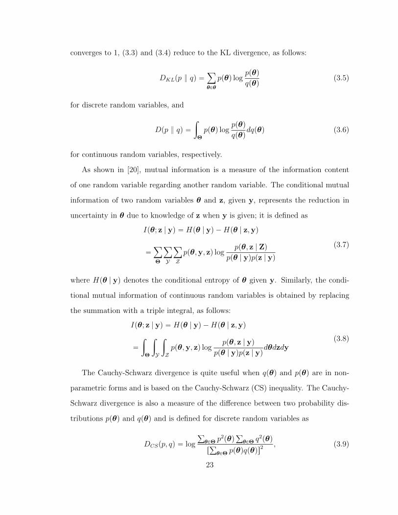
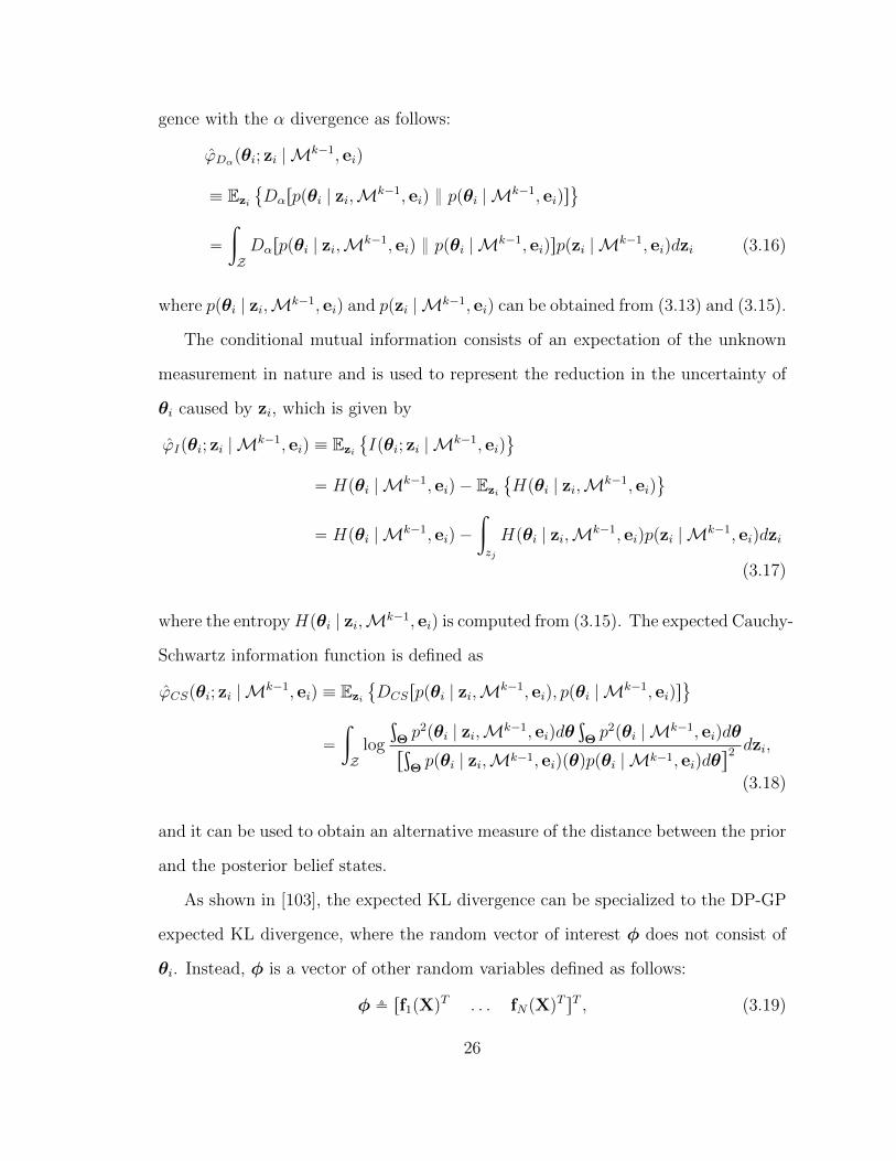
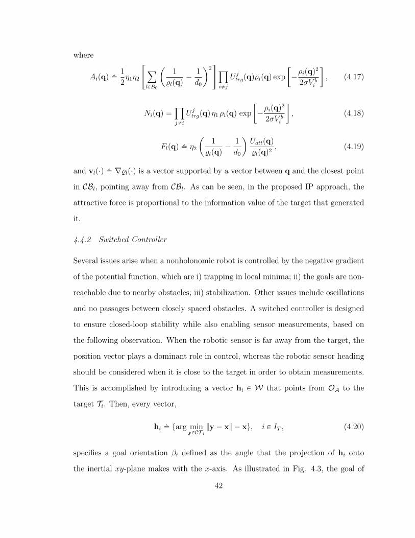
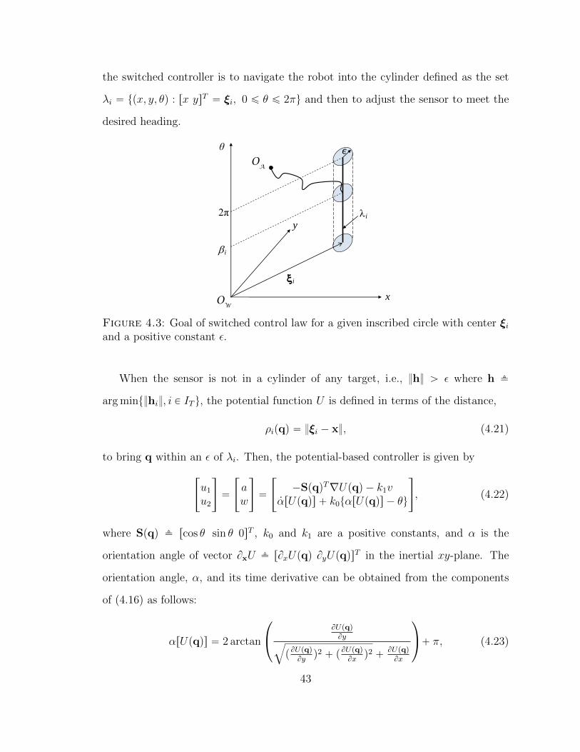
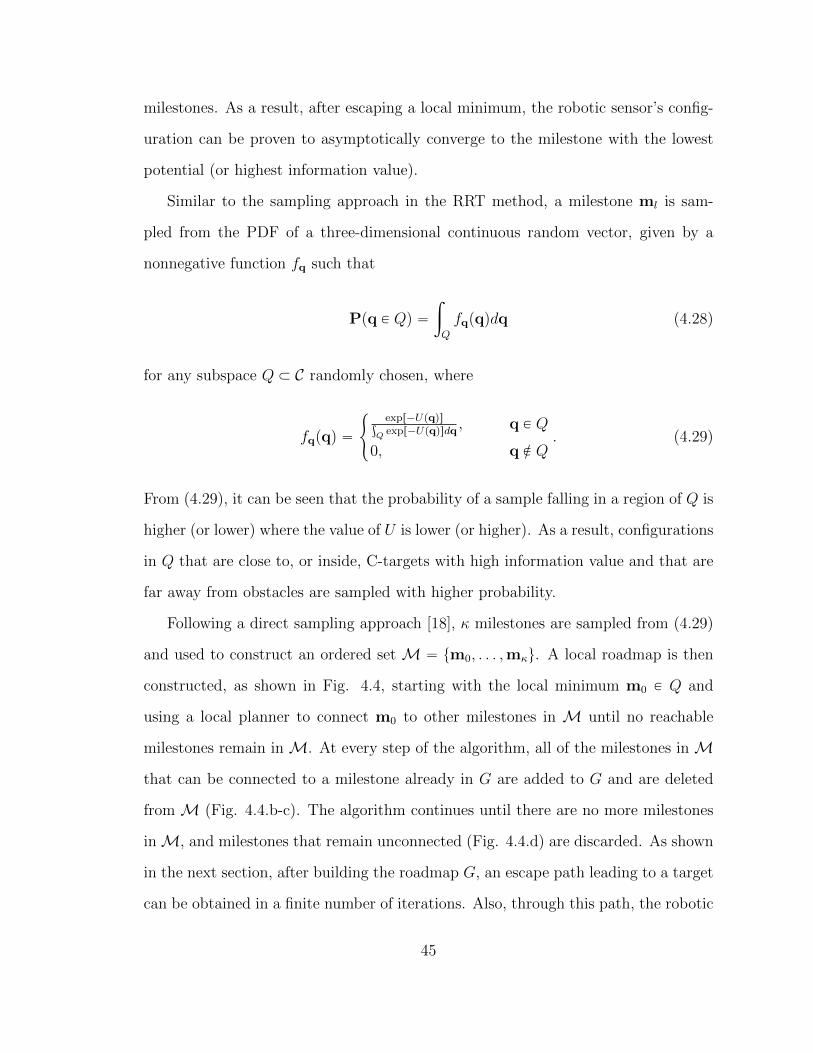
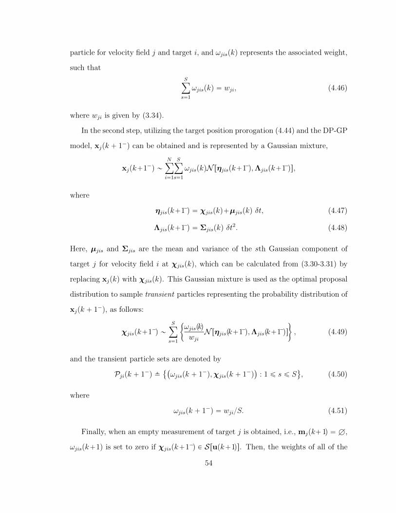
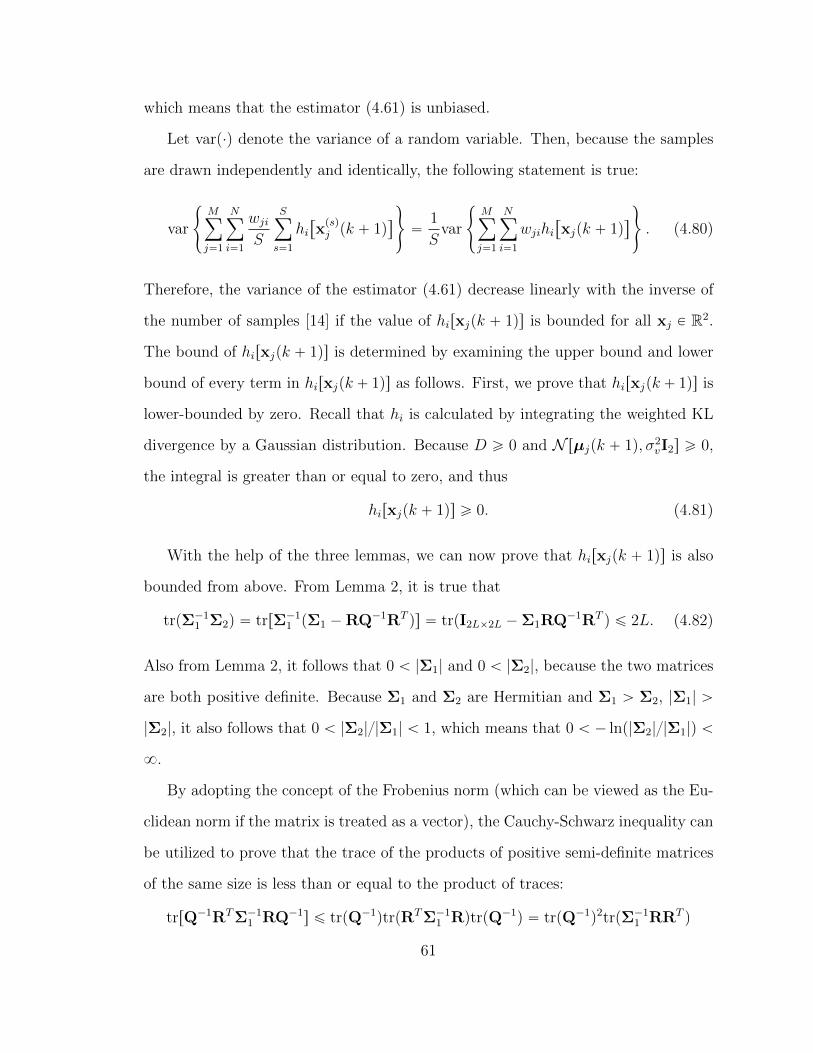
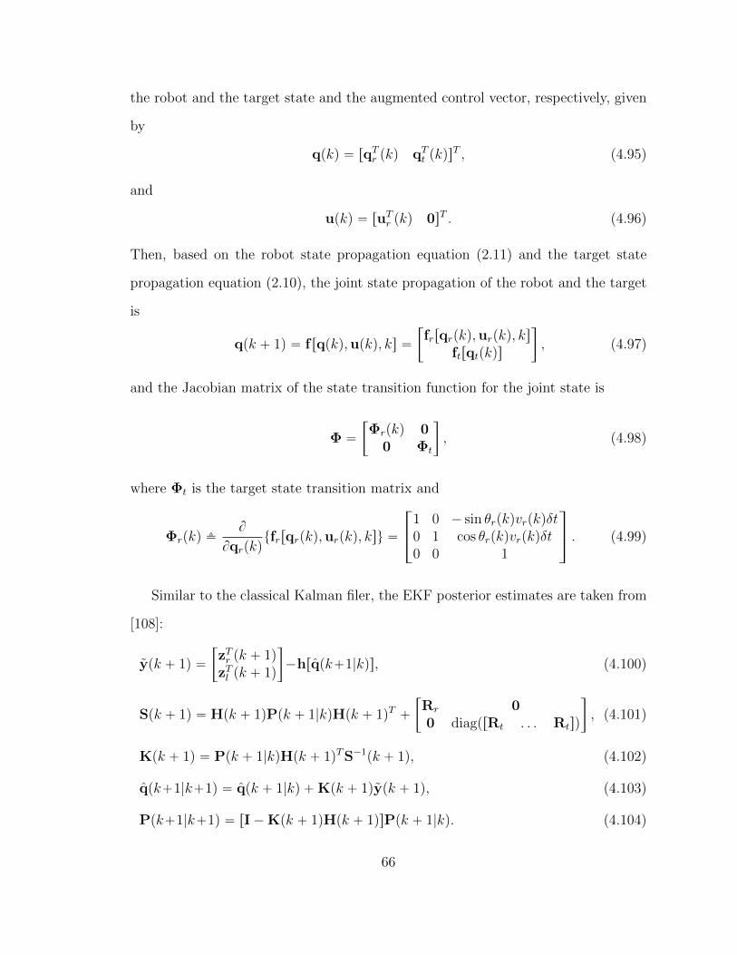
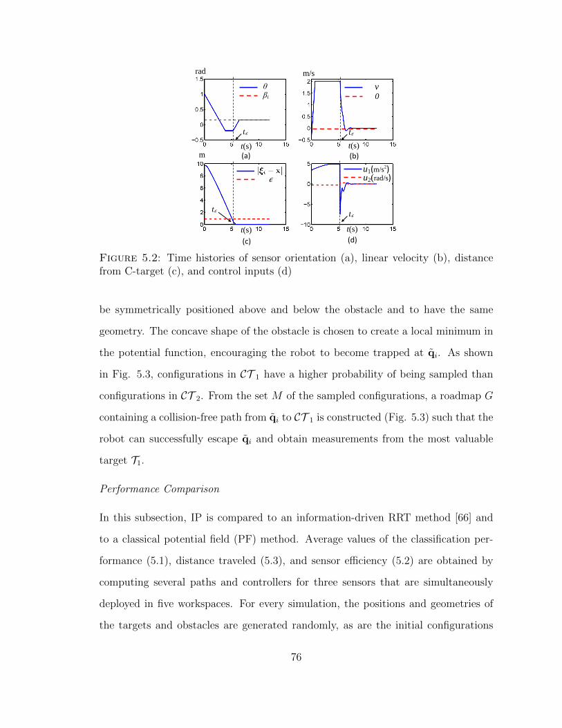
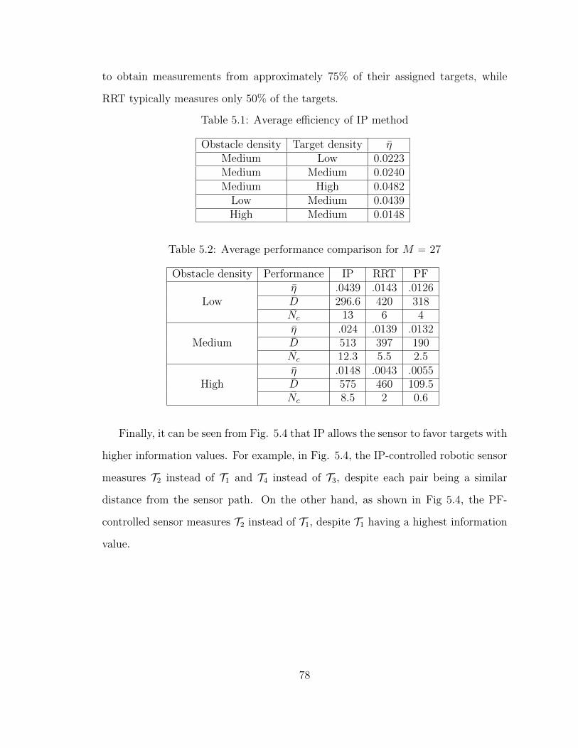
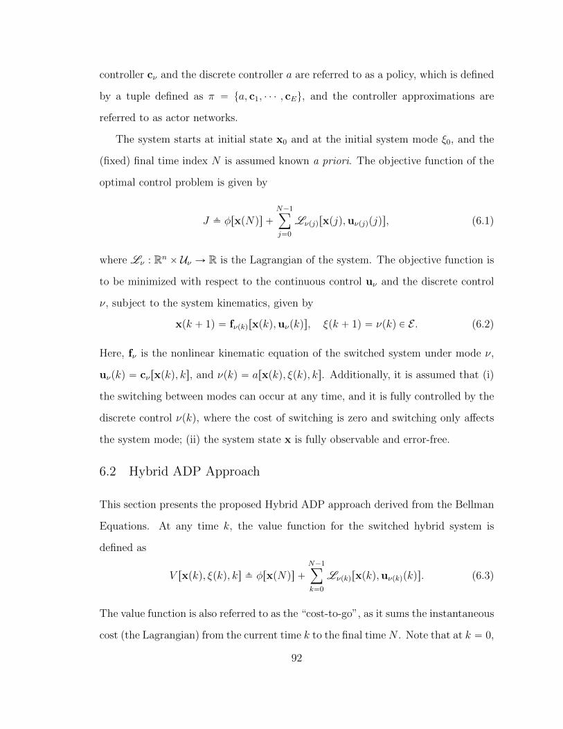
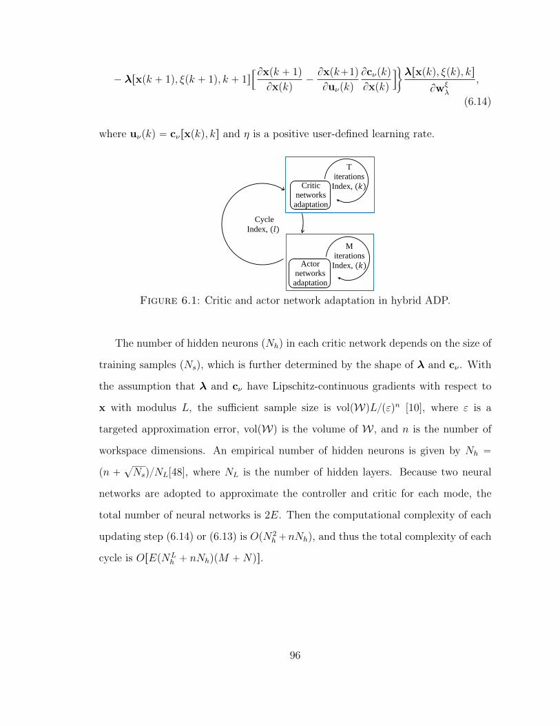
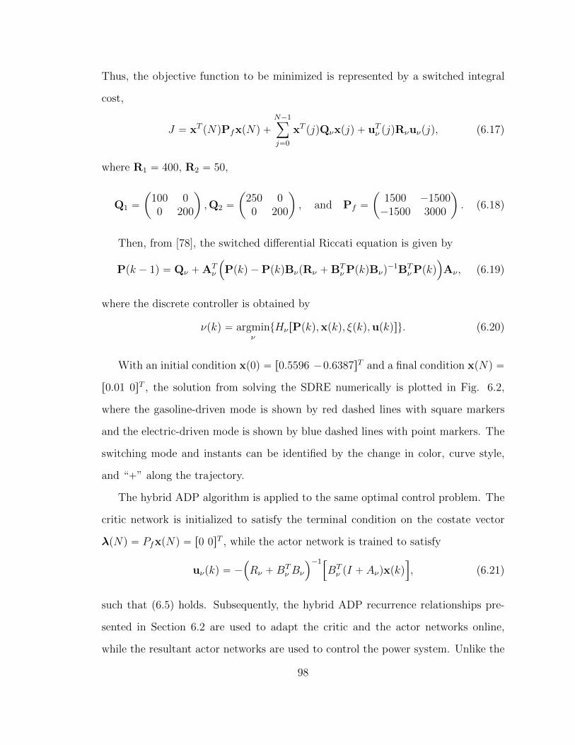
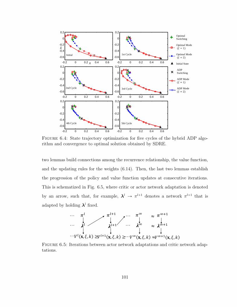
123