17
Lecture Note: Market Signaling — Theory and Evidence David H. Autor MIT 14.661 Fall 2003 November 17, 2003 1
| Date post: | 05-Apr-2018 |
| Category: |
Documents |
| Upload: | mervin-soldmervin |
| View: | 218 times |
| Download: | 0 times |

7/31/2019 Autor Signaling Notes
http://slidepdf.com/reader/full/autor-signaling-notes 1/17
Lecture Note: Market Signaling — Theory and Evidence
David H. AutorMIT 14.661 Fall 2003
November 17, 2003
1

7/31/2019 Autor Signaling Notes
http://slidepdf.com/reader/full/autor-signaling-notes 2/17
1 Introduction
George Akerlof’s 1970 paper on ‘Lemons’ was the first to formalize the adverse selection prob-
lem. Three key ingredient of this paper are:
1. Goods on the market are of heterogeneous quality
2. Sellers are better informed than buyers about the quality of their goods
3. Sellers have a reservation price for their goods
It is this reservation price that generates an adverse selection equilibrium. In particular,
Akerlof’s model shows that one can have a market equilibrium with no trade even when:
1. Every seller wants to sell at a positive price
2. There are buyers willing to pay the seller’s reservation price for each good
The reason that no trade may occur despite these conditions is that sellers hold reservation
prices above the price buyers are willing to pay for the goods available at that price. Because
the owner of an inferior good will always be willing to sell for the price of a superior good,
their is adverse selection of the goods for sale at a given price. In the extreme case, there is no
equilibrium price where the value of goods on the market at given price is equal to that price.
1.1 Review: The Akerlof model
A simple example.
• There are 2 types of new cars available at dealerships: good cars and lemons, which break
down often.
• The fraction of lemons at a dealership is λ.
• Dealers do not distinguish among good cars versus lemons — they sell what’s on the lot
at the sticker price.
2

7/31/2019 Autor Signaling Notes
http://slidepdf.com/reader/full/autor-signaling-notes 3/17
• Buyers cannot tell good cars from lemons, but they know that some fraction λ will be
lemons.
• After buyers have owned the car for any period of time, they can tell whether or not theyhave bought a lemon.
• Assume that good cars are worth $2, 000 and lemons are worth $1, 000.
• For simplicity (and without loss of generality), assume that cars do not deteriorate and
that buyers are risk neutral.
What is the equilibrium price for new cars? Clearly this must be
P N = (1 − λ) · 2, 000 + λ · 1, 000.
Since dealers sell all cars at the same price, buyers pay the expected value of a new car.
Now, consider the used car market. Assume that used car sellers are willing to part with
their cars at 20% below their new value. So,
P U G = $1, 600 and P U L = $800.
• Since cars don’t deteriorate, used car buyers will be willing to pay $2, 000 and $1, 000
respectively for used good cars and lemons. There is a $400 or $200 gain from trade from
each sale.
What is the equilibrium price of used cars?
• The natural answer is
P U = (1 − λ) · 1, 600 + λ · 800,
but this is not necessarily correct.
• Recall that buyers cannot distinguish good cars from lemons whereas owners of used cars
know which is which. Assuming sellers are profit maximizing, this means that at any
P U ≥ 800, owners of lemons will gladly sell them. But at P U < 1, 600, owners of good
cars will keep their cars.
3
7/31/2019 Autor Signaling Notes
http://slidepdf.com/reader/full/autor-signaling-notes 4/17
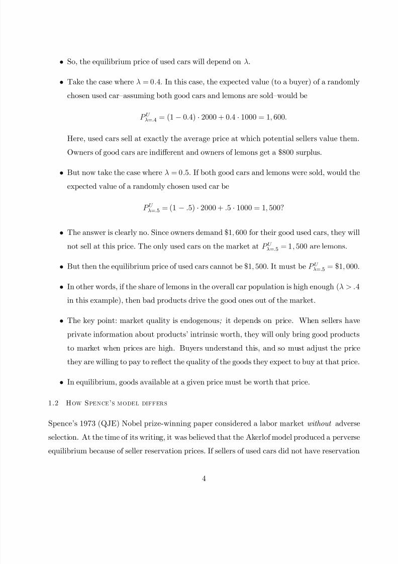
• So, the equilibrium price of used cars will depend on λ.
• Take the case where λ = 0.4. In this case, the expected value (to a buyer) of a randomly
chosen used car—assuming both good cars and lemons are sold—would be
P U λ=.4
= (1− 0.4) · 2000 + 0.4 · 1000 = 1, 600.
Here, used cars sell at exactly the average price at which potential sellers value them.
Owners of good cars are indiff erent and owners of lemons get a $800 surplus.
• But now take the case where λ = 0.5. If both good cars and lemons were sold, would the
expected value of a randomly chosen used car be
P U λ=.5
= (1 − .5) · 2000 + .5 · 1000 = 1, 500?
• The answer is clearly no. Since owners demand $1, 600 for their good used cars, they will
not sell at this price. The only used cars on the market at P U λ=.5
= 1, 500 are lemons.
• But then the equilibrium price of used cars cannot be $1, 500. It must be P U λ=.5
= $1, 000.
• In other words, if the share of lemons in the overall car population is high enough (λ > .4
in this example), then bad products drive the good ones out of the market.
• The key point: market quality is endogenous; it depends on price. When sellers have
private information about products’ intrinsic worth, they will only bring good products
to market when prices are high. Buyers understand this, and so must adjust the price
they are willing to pay to reflect the quality of the goods they expect to buy at that price.
• In equilibrium, goods available at a given price must be worth that price.
1.2 How Spence’s model differs
Spence’s 1973 (QJE) Nobel prize-winning paper considered a labor market without adverse
selection. At the time of its writing, it was believed that the Akerlof model produced a perverse
equilibrium because of seller reservation prices. If sellers of used cars did not have reservation
4

7/31/2019 Autor Signaling Notes
http://slidepdf.com/reader/full/autor-signaling-notes 5/17
prices that depended positively on their cars’ quality, then all goods would enter the market
simultaneously, and adverse selection would be eliminated. Problem solved?
This observation is partly correct — the no trade result depends on these reservation prices.
But Spence noticed that a perverse outcome is still possible even absent reservation prices.
If owners of superior goods (let’s say better workers) can take observable actions that less-
able workers cannot, they will often choose to do it, and wages will be paid diff erentially for
this observed characteristic. Spence’s insight was that these actions can occur in equilibrium,
even if they are costly and unproductive. Trade may occur with gross inefficiencies because of
unproductive signaling.
The Spence paper is quite simple, and the model would not pass muster in an advanced
undergraduate game theory class nowadays. But that doesn’t detract from the insight. For
edification, let’s do a modern, continuous version of the Spence model.
1.3 A signaling model — Separating equilibrium with many ability types
Let’s consider a labor market with a continuum of types θ ∈ £θ, θ̄
¤. The productivity of each
type θ is θ. Each type θ must choose an education level e. The endogenous variables (actually
functions) in these model will be w (e) and e∗ (θ). These are the wage for a given education
level and the optimal choice of education for each value of θ.
• The Worker’s Problem: Each θ will maximize over e.
maxe
w(e) − c (e, θ) ⇒ (1)
∂w (e∗)
∂e− ce (e∗, θ) = 0, ∀ θ.
• The Firm’s Problem: Assuming that the first condition results in a distinct e for each θ,
it needs to be the case that wages w (e) equal productivity at every e.
w (e∗ (θ)) = θ, ∀ θ, (2)
where e∗ (θ) is the solution to (1). Notice that because employers cannot observe θ, the
wage schedule must be entirely a function of e, which will itself depend on θ and on w (e).
5

7/31/2019 Autor Signaling Notes
http://slidepdf.com/reader/full/autor-signaling-notes 6/17
• So, we have two unknown functions: e∗ (θ), w (e∗ (θ)).
• Let’s solve a concrete example. Assume
c (e, θ) = k eθ
, (3)
k > 0, and θ= 1. Assume also that the lowest type gets no education: e (θ) = e (1) = 0.
(Probably a costless normalization.)
• The crucial feature of this cost function (3) is that its degree of convexity is declining in
θ. The higher is θ, the lower is the cost of education and the less rapidly its cost rises:
cθ =
−k
e
θ
2< 0, ce =
k
θ> 0, ceθ =
−
k
θ
2< 0.
• Applying the cost function to the worker’s problem, equation (1), we get
∂w
∂e=
k
θ.
• Applying the cost function to the firm’s problem, (2), we get
∂w
∂e·
∂e∗
∂θ= 1.
In words, worker ability must increase 1-for-1 with wages — otherwise wages are too highor too low.
• Putting put these conditions together gives,
∂e∗
∂θ=
θ
k.
• We now have the derivative but not the function. To find e∗ (θ), we need to integrate the
derivative from θ to θ:
e∗ (θ)− e∗ (θ) =Z
θ
θ
θk
dθ = θ2
2k− θ2
2k.
• Recalling that the lowest type gets no education (e∗ (θ) = 0) and that θ= 1, we obtain an
expression for e∗ (θ):
e∗ (θ) =θ2
2k− 1
2k.
6

7/31/2019 Autor Signaling Notes
http://slidepdf.com/reader/full/autor-signaling-notes 7/17
• Finally, we can obtain the function w (e) by inverting e∗ (θ) to get the expectation of
θ as a function of observable expectation and substitute this back into the equilibrium
expressions.
e = e∗ (θ) =θ2
2k− 1
2k,
w (e∗ (θ)) = E (θ|e) =p
e∗ (θ) 2k + 1.
• Note that this solution depended on the existence of a complete separating equilibrium:
each ability level θ gets a diff erent e∗. This equilibrium need not exist for all problems.
• [Algebra check. Take k = 1
2⇒ c(e) = 1
2
e
θ, w(e) =
√ e + 1.
e∗ (1) = 0, e∗ (2) = 3,
w∗ (0) = 1, w∗(3) = 2.
Now check the self-selection (‘separating’) constraints: Does any θ wish to change her
education level? Recall that cost of education is k e
θ.
w (3)− c (3, 1) = 2− 3/2 = 1/2 < w (0)− c (0, 1) = 1,
w (3)
−c (3, 2) = 2
−3/4 = 5/4 > w (0)
−c (0, 2) = 1.
The equilibrium functions work.]
• Hence, an equilibrium must have:
— Rational expectations: Along the equilibrium wage schedule, firms receive workers
whose productivity is equal to the wage they are paid.
— Self-selection: Workers have no incentive to take actions that would cause produc-
tivity to deviate from the wage schedule.
2 Empirical tests of market signaling
• Does the signaling model share any implications with the Human Capital model?
1. People who attend additional years of schooling are more productive. YES.
7

7/31/2019 Autor Signaling Notes
http://slidepdf.com/reader/full/autor-signaling-notes 8/17
2. People who attend additional years of schooling receive higher wages. YES.
3. The rate of return to schooling should be roughly equal to the rate of interest. NO
PREDICTION.
4. People will attend school while they are young, i.e., before they enter the workforce.
YES.
• How do you empirically distinguish the human capital and signaling models?
1. Measure whether more educated people are more productive? (Would be true for
either model.)
2. Measure people’s productivity before and after they receive education — see if it
improves. (Conceptually okay, very difficult to do.)
3. Test whether higher ability people go to school? (Could be true in either case—
certainly true in the signaling case.)
4. Find people of identical ability and randomly assign some of them to go to college.
Check if the college educated ones earn more? (Both models say they would.)
5. Find people of identical ability and randomly assign them a diploma. See if the ones
with the diploma earn more. (A pure test of signaling.)
• Because their empirical implications appear so similar, many economists had begun to
conclude that these models could not be empirically distinguished. The empirical papers
on the syllabus by Lang and Kropp (1986) and Bedard (2001) off er some evidence. Weiss
(1995) provides a survey.
• Both of the empirical papers implement closely related indirect tests of the signaling
model along the following lines. If we are initially at a separating equilibrium, how does
an exogenous decline in the cost of schooling for one group aff ect the education choices of
other worker groups who are not directly aff ected by the price change? Lang and Kropp
look at college going as a function of school leaving laws (which primarily directly aff ect
secondary school attendance). Bedard looks at high school dropout rates as a function of
8

7/31/2019 Autor Signaling Notes
http://slidepdf.com/reader/full/autor-signaling-notes 9/17
the cost of attending college. Both purport to find that the ‘indirectly aff ected groups’
behave as the signaling model would predict: students attend college to ‘separate’ from
the high school grads (Lang and Kropp); more students drop out of high school because
the quality of the high school graduate pool is diluted by greater college attendance —
and so its not worth the cost of education to pool with them (Bedard).
• These tests are pretty weak — the empirical equivalent of aiming for the capillaries. They
indirectly test second order predictions of the signalling model.
• A first order prediction of the model is this: A ‘signal’ (such as education) commands a
positive price in equilibrium, even when acquiring that signal has no impact on human
capital production. To test this prediction, one would have to randomly assign signals
to individuals of otherwise identical expected productivity. Tyler, Murnane and Willett
identify one such quasi-experiment.
3 The Tyler, Murnane and Willett study
• TMW are interested in knowing whether the General Educational Development certificate
(GED) raises the subsequent earnings of recipients.
• This question is important for educational policy:
— By 1996, 9.8% of those ages 18 − 24 had completed High School via the the GED
versus 76.5% via a HS diploma.
— See Table I. Notice that between 1990 and 1996, HS Diploma rates actually fell
dramatically for Black, Non-Hispanics. The rise in the GED just off set this. Hence,
we ought to hope that these GED holders are doing at least somewhat better than
HS dropouts.
• In 1996, 759, 000 HS Dropouts attempted the GED and some 500, 000 passed.
• The monetary cost of taking the GED is $50 and the exam lasts a full day.
9
7/31/2019 Autor Signaling Notes
http://slidepdf.com/reader/full/autor-signaling-notes 10/17
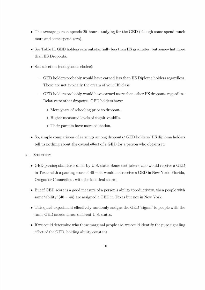
• The average person spends 20 hours studying for the GED (though some spend much
more and some spend zero).
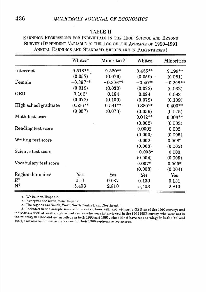
• See Table II. GED holders earn substantially less than HS graduates, but somewhat morethan HS Dropouts.
• Self-selection (endogenous choice):
— GED holders probably would have earned less than HS Diploma holders regardless.
These are not typically the cream of your HS class.
— GED holders probably would have earned more than other HS dropouts regardless.
Relative to other dropouts, GED holders have:
∗ More years of schooling prior to dropout.
∗ Higher measured levels of cognitive skills.
∗ Their parents have more education.
• So, simple comparisons of earnings among dropouts/ GED holders/ HS diploma holders
tell us nothing about the causal eff ect of a GED for a person who obtains it.
3.1 Strategy
• GED passing standards diff er by U.S. state. Some test takers who would receive a GED
in Texas with a passing score of 40− 44 would not receive a GED in New York, Florida,
Oregon or Connecticut with the identical scores.
• But if GED score is a good measure of a person’s ability/productivity, then people with
same ‘ability’ (40− 44) are assigned a GED in Texas but not in New York.
• This quasi-experiment eff ectively randomly assigns the GED ‘signal’ to people with the
same GED scores across diff erent U.S. states.
• If we could determine who these marginal people are, we could identify the pure signaling
eff ect of the GED, holding ability constant.
10

7/31/2019 Autor Signaling Notes
http://slidepdf.com/reader/full/autor-signaling-notes 11/17
• What does the signaling model predict in this case?
• Since some dropouts obtain the GED and some do not, it’s plausible that the market is
in some type of ‘separating’ equilibrium (i.e., not everyone gets the signal).
• For the GED to perform as a signal, it needs to be the case that the cost of obtaining it
is lower for more productive workers (otherwise everyone or no one would get it). This
seems plausible; you cannot pass the GED without some education and study.
• In equilibrium, the following must be true for individuals:
wGED − wNO−GED ≥ C GED ⇒ obtain,
wGED − wNO−GED < C GED ⇒ don’t obtain,
where C GED is the direct and indirect costs of obtaining the GED.
• And the following must be true for employers:
wGED = E (Productivity|C GED ≤ wGED − wNO−GED),
wNO−GED = E (Productivity|C GED > wGED − wNO−GED).
• If these conditions are satisfied, firms will be willing to pay the wages wGED , wNO−GED to
GED and non-GED holders respectively, and workers will self-select to obtain the GED
accordingly.
• We are assuming that firms cannot observe worker ability independent of the GED.
• So, given the quasi-experimental setup, the signaling model predicts that workers with
GED scores of 40
−44 will earn more if they receive the GED certificate than if they do
not.
• By contrast, the Human Capital model implies that since ability is comparable among
these groups, wages will also be comparable.
11

7/31/2019 Autor Signaling Notes
http://slidepdf.com/reader/full/autor-signaling-notes 12/17
3.2 Difference-in-difference
• The econometric strategy for this paper is similar to the Card-Krueger minimum wage
study: diff
erences-in-diff
erences.
• TMW choose a control group of GED test takers with scores just about the cutoff for
both groups of states. Hence, the GED treatment works as follows:Low Passing Standard High Passing Standard
Low Score (treatment group) GED NO GEDHigh Score (control group) GED GED
• The outcome variable will be earnings for each of these four groups:Low Passing Standard High Passing Standard
Low Score (treatment group) $L, L $L, H High Score (control group) $L, H $H, H
• Notice the following contrasts
(1) $L, L− $L, H = earnings diff of GED/non-GED holders with same scores.
(2) $L, H − $H, H = earnings diff of GED holders with same scores across these states.
(1)− (2) = diff erence-in-diff erence estimate (netting out state diff s)
• See Table V.
• See Figures I-III.
3.3 TMW: Conclusions
• Large signaling eff ects for whites, estimated at 20% earnings gain after 5 years.
• Does this prove that GED holders are not more productive than non-GED holders?
— No. Just the opposite.
— For there to be a signaling equilibrium, it must be the case that GED holders are
on average more productive than otherwise similar HS dropouts who do not hold a
GED.
• Do these results prove that the GED is productive?
12
7/31/2019 Autor Signaling Notes
http://slidepdf.com/reader/full/autor-signaling-notes 13/17
— No. They are not inconsistent with that fact, but they off er no evidence one way or
another.
• Do these results prove that education is unproductive?
— No, they also have nothing to say on this because education/skill is eff ectively hold
constant by this quasi-experiment.
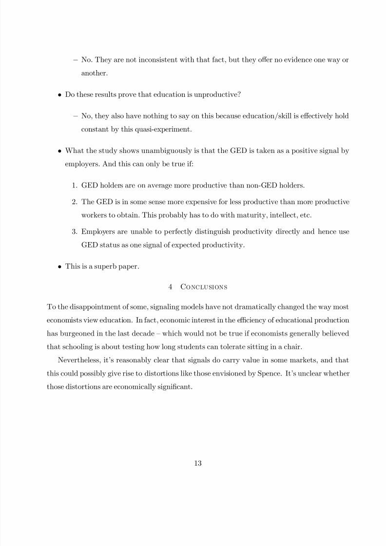
• What the study shows unambiguously is that the GED is taken as a positive signal by
employers. And this can only be true if:
1. GED holders are on average more productive than non-GED holders.
2. The GED is in some sense more expensive for less productive than more productive
workers to obtain. This probably has to do with maturity, intellect, etc.
3. Employers are unable to perfectly distinguish productivity directly and hence use
GED status as one signal of expected productivity.
• This is a superb paper.
4 Conclusions
To the disappointment of some, signaling models have not dramatically changed the way most
economists view education. In fact, economic interest in the efficiency of educational production
has burgeoned in the last decade — which would not be true if economists generally believed
that schooling is about testing how long students can tolerate sitting in a chair.
Nevertheless, it’s reasonably clear that signals do carry value in some markets, and that
this could possibly give rise to distortions like those envisioned by Spence. It’s unclear whether
those distortions are economically significant.
13

7/31/2019 Autor Signaling Notes
http://slidepdf.com/reader/full/autor-signaling-notes 14/17
7/31/2019 Autor Signaling Notes
http://slidepdf.com/reader/full/autor-signaling-notes 15/17

7/31/2019 Autor Signaling Notes
http://slidepdf.com/reader/full/autor-signaling-notes 16/17

7/31/2019 Autor Signaling Notes
http://slidepdf.com/reader/full/autor-signaling-notes 17/17


![[Nome completo do autor] [Habilitações Académicas] [Nome ... · Diogo Rodrigues Francisco Sabino [Nome completo do autor] [Nome completo do autor] [Nome completo do autor] Hydrogels](https://static.documents.pub/doc/80x56/60e4508f8c055874545babee/nome-completo-do-autor-habilitaes-acadmicas-nome-diogo-rodrigues.jpg)


