Average versus high s urface ozone levels over the ... · Chem global chemistry ... surfa ce O 3...

1

Average versus high surface ozone levels over the continental

U.S.A.: Model bias, background influences, and interannual

variability

Jean J. Guo1, Arlene M. Fiore1, Lee T. Murray2,3,4, Daniel A. Jaffe5, Jordan L. Schnell6,7, Tom 5

Moore8, George Milly2

1Department of Earth and Environmental Sciences and Lamont-Doherty Earth Observatory of Columbia University,

Palisades, NY, U.S.A. 2Lamont-Doherty Earth Observatory of Columbia University, Palisades, NY, U.S.A.

3NASA Goddard Institute for Space Studies, New York, NY USA 10 4Now at: Department of Earth and Environmental Sciences, University of Rochester, Rochester, NY, U.S.A. 5University of Washington, School of STEM, Bothell, WA and Department of Atmospheric Science, Seattle, WA,

U.S.A. 6NOAA Geophysical Fluid Dynamics Laboratory, Atmospheric and Oceanic Sciences, Princeton University,

Princeton, NJ, U.S.A. 15 7Now at: Department of Earth and Planetary Sciences, Northwestern University, Chicago, IL, U.S.A. 8WESTAR and WRAP, Colorado State University, Fort Collins, CO, U.S.A.

Correspondence to: Jean J. Guo ([email protected])

Abstract. U.S. background ozone (O3) includes O3 produced from anthropogenic O3 precursors emitted outside of the

U.S.A., from global methane, and from any natural sources. Using a suite of sensitivity simulations in the GEOS-20

Chem global chemistry-transport model, we estimate the influence from individual background versus U.S.

anthropogenic sources on total surface O3 over ten continental U.S. regions from 2004-2012. Evaluation with

observations reveals model biases of +0-19 ppb in seasonal mean maximum daily 8-hour average (MDA8) O3, highest

in summer over the eastern U.S.A. Simulated high-O3 events cluster too late in the season. We link these model biases

to regional O3 production (e.g., U.S. anthropogenic, biogenic volatile organic compounds (BVOC), and soil NOx, 25

emissions), or coincident missing sinks. On the ten highest observed O3 days during summer (O3_top10obs_JJA), U.S.

anthropogenic emissions enhance O3 by 5-11 ppb and by less than 2 ppb in the eastern versus western U.S.A. The O3

enhancement from BVOC emissions during summer is 1-7 ppb higher on O3_top10obs_JJA days than on average

days, while intercontinental pollution is up to 2 ppb higher on average vs on O3_top10obs_JJA days. In the model,

regional sources of O3 precursor emissions drive interannual variability in the highest observed O3 levels. During the 30

summers of 2004-2012, monthly regional mean U.S. background O3 MDA8 levels vary by 10-20 ppb. Simulated

summertime total surface O3 levels on O3_top10obs_JJA days decline by 3 ppb (averaged over all regions) from 2004-

2006 to 2010-2012 in both the observations and the model, reflecting rising U.S. background (+2 ppb) and declining

U.S. anthropogenic O3 emissions (-6 ppb). The model attributes interannual variability in U.S. background O3 on

Atmos. Chem. Phys. Discuss., https://doi.org/10.5194/acp-2018-115Manuscript under review for journal Atmos. Chem. Phys.Discussion started: 26 February 2018c© Author(s) 2018. CC BY 4.0 License.

2

O3_top10obs days to natural sources, not international pollution transport. We find that a three-year averaging period 35

is not long enough to eliminate interannual variability in background O3.

1 Introduction

In the United States, ozone (O3) is regulated as a criteria pollutant under the National Ambient Air Quality

Standard (NAAQS). The current NAAQS for ground-level O3, set in October 2015, states that the 4th-highest daily

maximum 8-hour average (MDA8) O3, averaged across three consecutive years, cannot be 71 ppb or higher (U.S. 40

Environmental Protection Agency, 2015). The three-year average is nominally intended to smooth out fluctuations

in O3 levels resulting from natural variability in meteorology, within the timing constraints of the federal Clean Air

Act for air quality planning. As even one ppb of excess O3 may be enough to push a county out of NAAQS

attainment, it is relevant to understand which sources influence the severity and timing of the highest O3 events. As

measured O3 does not retain a signature of the source from which it was produced, estimates of background O3 rely 45

on models, ideally evaluated closely with observational values, to build confidence in the model capability for

source attribution. Here we apply a global chemistry-transport model alongside O3 observations to examine the

highest 10 observed O3 events, as well as average conditions, to determine which sources are influencing average

versus high-O3 events, and the extent to which they vary from year-to-year.

As U.S. anthropogenic emissions of O3 precursors decline, the relative importance of “U.S. background” to 50

total surface O3 rises. U.S. background O3 is defined here as the O3 levels that would exist in the absence of U.S.

anthropogenic emissions of O3 nitrogen oxide (NOx) and non-methane volatile organic compound (NMVOC)

precursors. U.S. background O3 thus includes naturally occurring O3 as well as O3 produced from global methane

(including U.S. anthropogenic emissions) and from O3 precursor emissions outside of the U.S.A. Jaffe et al. (2018)

review the current understanding on U.S. background O3 from models and observations, and its relevance to air quality 55

standard setting and implementation. Previous studies estimating background O3 over the United States found that

background sources of O3, including stratospheric O3 intrusions (Lin et al., 2012, 2015a), increasing Asian

anthropogenic emissions (Lin et al., 2015b), and more frequent wildfires in summer (Abatzoglou and Williams, 2016;

Jaffe, 2011; Yang et al., 2015), may present challenges to obtaining the O3 standard, especially since regional emission

controls may be offset by a warming climate (Fiore et al., 2015). At high-altitude Western U.S. (WUS) sites in spring, 60

the influence from stratospheric intrusions and foreign transport, combined with relatively deep planetary boundary


3

layers, can lead to high background O3 events (Fiore et al., 2002; Zhang et al., 2011). Lin et al. (2017) investigated

surface O3 trends over the U.S.A. from 1980-2014 with the GFDL AM3 model and found that emissions controls

decreased the 95th percentile summer O3 values in the Eastern U.S. (EUS) by 0.2-0.4 ppb yr-1 over 1988-2014, but

rising Asian emissions offset the effect of U.S. emissions reductions, leading to 2-8 ppb increases in monthly mean 65

O3 at individual sites in the WUS (Lin et al., 2016).

Earlier work in the GEOS-Chem model analyzing background O3 during a single meteorological year noted

a tendency for the model to underestimate springtime O3 at high-altitude WUS sites but overestimate summertime

O3 over the EUS (e.g. Fiore et al., 2002, 2003; Wang et al., 2009; Zhang et al., 2011, 2014). Identifying the extent to

which these biases reflect poor representation of U.S. anthropogenic versus background sources is relevant for 70

assessing uncertainties in estimates of background O3 on days when the O3 NAAQS is exceeded. We build upon

these prior studies by analyzing MDA8 O3 measurements and 9-year model simulations spanning 2004-2012 from

the GEOS-Chem 3D global chemistry-transport model (CTM). We use a suite of GEOS-Chem sensitivity

simulations to estimate the influence from various individual background sources on O3 concentrations and the

interannual variability in background O3 levels, with a focus on the highest 10 events in each EPA region during 75

each summer (JJA) or year. We aim to answer the following questions: (1) Which sources exert the strongest

influence on O3 on the ten days with the highest model biases against observations? (2) Which background sources

influence total O3 the most on average versus the 10 highest O3 days? (3) Which sources influence the interannual

variability of O3 in each region on average versus the 10 highest O3 days?

2 Observations and model simulations 80

2.1 Observations

We use observed 2004-2012 MDA8 O3 data from the EPA Air Quality System (AQS) network of urban,

suburban, and rural monitoring sites, the Clean Air Status and Trends Network (CASTNet), and the Mount Bachelor

Observatory

(https://digital.lib.washington.edu/researchworks/browse?type=subject&value=Mt.+Bachelor+Observatory) in 85

Oregon. MDA8 O3 values for the AQS sites were download from

http://aqsdr1.epa.gov/aqsweb/aqstmp/airdata/download_files.html#Daily (2004-2012 data last updated June 28,

2013). This dataset includes 1644 total sites from the contiguous U.S.A. from 2004-2012 with 1207 to 1333 sites


4

collecting data each year (U.S. Environmental Protection Agency, 2014) (Supplemental Figure 1). The number of

AQS sites measuring data per year is listed in Supplemental Figure 1. 90

The CASTNet (ftp://ftp.epa.gov/castnet/data) O3 monitoring sites are located in rural areas away from

emission sources and densely populated regions. CASTNet sites are designed to capture background O3 levels and

characterize the broad spatial and temporal trends of air pollutants. We calculate the MDA8 O3 concentration from

hourly values at 108 CASTNet sites with data between 2004-2012, requiring at least 18 hours of data per day for

each MDA8 O3 calculation. 95

The Mount Bachelor Observatory, established in 2004 by the University of Washington Jaffe Research

Group, is located 2.7 km above sea level on the summit of Mount Bachelor, an extinct volcano in the Cascade

Mountains of central Oregon. It provides an estimate of baseline O3 levels over the West Coast of the United States.

Baseline O3 is tropospheric O3 concentrations at sites that have a negligible influence from local emissions (National

Research Council, 2010). Here we take all hourly O3 concentrations from Mount Bachelor and calculate the MDA8 100

O3 concentrations for 2004-2012. Daily averages are included only if at least 18 hours of data are available per day.

As we did not archive three-dimensional high frequency data, all MDA8 O3 values from the model are sampled at

the lowest surface layer for comparison to observation sites. Monthly MDA8 O3 averages from Mount Bachelor are

included only if at least 20 days out of the month contain valid daily data. For our comparison to monthly mean

measurements at Mount Bachelor, we sample the model at the height closest to 2.7 km. 105

In order to evaluate the GEOS-Chem model O3 simulation (described below in Sect. 2.3) at a spatial scale

comparable to the coarse horizontal resolution global grid (2º x 2.5º), we use an available 1° x 1° grid of interpolated

surface MDA8 O3 measurements described by Schnell et al. (2014). We degrade the Schnell et al. (2014) dataset to

2° x 2.5° to match that of the GEOS-Chem simulations.

2.2 Analysis regions 110

Each observational site in the EPA AQS and CASTNet datasets is linked to one of the 10 EPA air quality

regions (Figure 1) based on which state the site is in. The Mount Bachelor data were included with the Region 10

(Pacific Northwest) sites (Table 2) as a station representative of variations in baseline O3 concentrations in the

U.S.A. (Baylon et al., 2016) even though it is not a regulatory monitor. Similar to Reidmiller et al. (2009), we select

two regions, the Southeast (Region 4) and Mountains and Plains (Region 8), as representative regions for the EUS 115


5

and WUS for illustration purposes in the main text. Figures showing our results for the other six regions are included

in the supplement.

We first match each observational site to the model grid within which it falls. We then average across all

sites in each region to obtain a regional MDA8 O3 value for each day. From the regionally averaged observed

MDA8 O3, we find: (1) the ten days with the highest observed O3 during each year (hereafter, O3_top10obs days; 120

similar to the definition for extreme events used in Schnell et al., 2014), (2) the ten days with the highest O3

observations during each season (hereafter, O3_top10obs_MAM, O3_top10obs_JJA, and O3_top10obs_SON), and

(3) the 4th highest MDA8 O3 within each year. In addition, we sample the model to find the ten days each year with

the highest positive biases. We use O3_top10obs as our primary metric instead of the policy-relevant 4th highest O3

because the model bias is comparatively lower; on the days with the 4th highest values, the model bias is generally 125

more strongly negative in the west and South Central regions and more strongly positive in the Midwest than on

O3_top10obs days (Supplemental Figure 1, Supplemental Figure 2). In addition, while the model rarely captures the

exact day of the 4th highest MDA8 O3 event, there is a 3-4 day overlap on average between the O3_top10obs days

and the highest 10 MDA8 O3 days in the model. This overlap is similar to the 3 and 6 day overlap Jaffe et al. (2017)

found in their regional models for May 1st to September 29th, 2011. 130

2.3 GEOS-Chem model simulations

We use the GEOS-Chem v9_02 global 3D chemical transport model (CTM) (http://www.geos-chem.org)

simulations driven by Modern-Era Retrospective analysis for Research and Applications (MERRA) reanalysis

meteorology from the NASA Global Modeling and Assimilation Office for 2004-2012 (Rienecker et al., 2011).

The MERRA reanalysis is available at 1/2º by 2/3º horizontal resolution, which we degrade here to 2º by 2.5˚ 135

horizontal resolution. Anthropogenic base emissions are from the Emission Database for Global Atmospheric

Research (EDGAR) version 3.2-FT2000 inventory (Olivier et al., 2005) for inorganic compounds and the

REanalysis of the TROpospheric chemical composition (RETRO) inventory (Hu et al., 2015; Schultz, 2007) for

organic compounds. Inorganic emissions are overwritten by regional inventories for the U.S. (EPA National

Emissions Inventory 2005), Canada (Criteria Air Contaminants), Mexico (Big Bend Regional Aerosol and 140

Visibility Observational study; Kuhns and Green, 2003), Europe (European Monitoring and Evaluation

Programme; Auvray and Bey, 2005), and South and East Asia (Streets et al., 2006). Separate global inventories are


6

used for ammonia (Bouwman et al., 1997), black carbon (Bond et al., 2007; Leibensperger et al., 2012), and ethane

(Xiao et al., 2008). Anthropogenic surface emissions have diurnal and monthly variability, some with additional

weekly cycles, and are scaled each year on the basis of economic data (Van Donkelaar et al., 2008). Aircraft 145

emissions are from the Avian Emissions Inventory Code (AEIC) inventory (Stettler et al., 2011) and shipping

emissions are from International Comprehensive Ocean-Atmosphere Data Set (ICOADS; Lee et al., 2011; Wang et

al., 2008). Biomass burning emissions follow the interannually-varying monthly Global Fire Emissions Database

version 3 (GFED3) inventory driven by satellite observations of fire activity (Giglio et al., 2010; Van Der Werf et

al., 2010). Biofuel emissions are constant (Yevich and Logan, 2003). Biogenic VOC emissions from terrestrial 150

plants follow the Model of Emissions of Gases and Aerosols from Nature (MEGAN) scheme version 2.1

(Guenther et al., 2012) and vary with meteorology (Barkley et al., 2011). Emissions of NOx from soil microbial

activity follow Hudman et al. (2012). Methane surface concentrations are prescribed each month using spatially

interpolated surface distributions from NOAA Global Monitoring Division flash data.

We first perform a base simulation (O3_Base) in which all emissions are prescribed normally for 2003-155

2012. We then perform parallel sensitivity simulations in which we remove individual sources (Table 1), including

(1) U.S. anthropogenic emissions, but maintaining present-day methane concentrations; the O3 in this simulation

provides an estimate of U.S. background O3 (hereafter, O3_USB); (2) an otherwise identical simulation that also

excludes those emissions from Mexico and Canada, O3 in this simulation is referred to as “North American

Background” O3 (O3_NAB); (3) wildfire emissions, (4) biogenic VOC emissions, (5) Soil NOx, and (6) Lightning 160

NOx. In addition, we perform a “natural” simulation in which all anthropogenic emissions have been removed

globally and methane is prescribed at preindustrial levels to provide an estimate of “natural” O3 (O3_NAT). In all

simulations, we discard 2003 from our analysis as initialization. We estimate the contribution of each individual

sector to the total concentration by subtracting the O3 in each sensitivity simulation in which that source has been

removed from the O3_Base simulation. As in all “zero-out” perturbation simulations, non-linearities in atmospheric 165

photochemistry make this a simple estimate of the contribution of each source, and the contribution of each source

depends on the presence of all other precursor emissions at present-day levels (e.g., the impact of BVOCs

emissions is sensitive to the amount of anthropogenic NOx emissions). Hereafter, the terms listed in the “Notation”

column of Table 1 will be used to refer to the influence of each source on total O3 (O3_Base). Note that this set of

model simulations does not directly isolate stratospheric O3 or Asian influences. Previous work has shown that 170


7

stratospheric O3 can increase O3 levels by 17-40 ppb in the WUS in spring when MDA8 O3 levels are 70-85 ppb,

and Asian emissions can contribute 8-15 ppb to MDA8 O3 on days above 60 ppb (Lin et al., 2012, 2015a).

Stratospheric and Asian influences are included as part of our O3_USB estimates; Asian influences are included in

O3_ICT+CH4, and O3_NAT contains the influence of stratospheric O3 along with natural biogenic precursor

emissions, wildfires, and lightning NOx. 175

3 Model evaluation

3.1 MDA8 O3 distributions

Previous studies have found that averaging all observational sites within a model grid cell tend to

disproportionately represent urban stations, especially when looking at high O3 days (Schnell et al., 2014). To

evaluate the ability of our coarse resolution model to capture observed high-O3 events, we compare the MDA8 O3 180

simulated by GEOS-Chem to the observations in two ways. First, we use the Schnell et al. (2014) gridded dataset

degraded to the model resolution. Second, we compare each individual observational site to the model grid cell

within which it resides. The model is biased positively with either method (Figure 2a, b), but the shape of the model

distribution constructed with the latter approach (Figure 2b) better matches the observed distribution than that of the

former (Figure 2a). Matching individual sites to the nearest model grid (Figure 2b) results in a better estimate of 185

high-O3 days; the model overestimates the percentage of days above 70 ppb by about three times when we match to

individual measurement sites (3.14% of days are above 70 ppb in the observations versus 9.92% in model) but by

about ten times in comparison to the re-gridded Schnell (2014) dataset (0.37% of days are above 70 ppb in the

observations versus 3.91% in the re-gridded dataset).

3.2 Baseline O3 at Mount Bachelor 190

Mount Bachelor Observatory is located at 2.7 km above sea level, where it regularly samples free

tropospheric O3 and is rarely influenced by local anthropogenic emissions (Reidmiller et al., 2009). It is therefore, a

valuable site for examining baseline O3 values. Figure 3 compares modeled and observed monthly mean O3 at

Mount Bachelor. The observations peak in springtime and then fall in the summer months. The model, however, has

a maximum in and underestimates springtime baseline O3. We infer, consistent with our analysis below, that the 195

model does not resolve springtime high-O3 events, possibly reflecting an underestimate of stratospheric influences

(see Fiore et al., 2014; Zhang et al., 2011; 2014). The model indicates that O3_USB dominates O3_Base (Figure 3).


8

Even at this baseline site, however, the model indicates that U.S. anthropogenic emissions enhance monthly mean

O3 by at least a few ppb (estimated as the difference between O3_Base and O3_USB).

3.3 Magnitude and timing of high-O3 events 200

Simulated seasonal mean MDA8 averaged over the full 2004-2012 period is higher than observed by 5-30

ppb (Figure 4a, b, c), with the largest biases typically occurring in the Northeast and Midwest. The model bias is

highest in summer (JJA) (15-30 ppb at most sites), followed by fall (SON) (10-20 ppb) (Figure 4a, b, c). Recent

work in a newer version of GEOS-Chem attributes some of the positive model bias in the EUS to excessive NOx

emissions in the 2011 National Emission Inventory (NEI) (Travis et al., 2016), an inability of the model to resolve 205

vertical mixing in the boundary layer, and a weak response to cloud cover (Travis et al., 2017). The model is closest

to the observations in spring, with a positive bias usually <10 ppb over the eastern states and generally within ±5

ppb over most western sites (Figure 4a, b, c). On O3_top10obs days, however, biases are typically lower than on

average days (Figure 4, Table 3; see also year-by-year maps in Supplemental Figure 1). At some WUS sites, the

model underestimates O3 levels during the highest events by 10-20 ppb. We note that the model systematically 210

underestimates O3 in the Central Valley of California in all three seasons, which we attribute to the inability of the

coarse model resolution to resolve topographical gradients and valley circulations (or stagnation) in this region

which experiences some of the highest observed O3 in the nation.

We compare the MDA8 O3 distributions in the observations versus the model (O3_Base) during the 10

most biased days in each of the ten regions across the nine years (900 total events). These “most-biased” days in 215

the model tend to fall around the observed median (Figure 2c) during the warm season (June - October), with

almost 40% of the days falling in August alone (Figure 5), and are 9-45 ppb higher than the observations (circles in

Figure 6, Supplemental Figure 3). We analyze the perturbation simulations (Table 1) to identify which sources

influence simulated O3 most strongly on the “most-biased” days versus on average (i.e., all 365 or 366 days),

which we assume are also likely the main drivers of the bias. In all regions, the largest sources on the “most-220

biased” model days are O3_USA (3-30 ppb higher MDA8 O3 than on average with the exception of the Pacific SW

where O3_USA is smaller than on average days), O3_BVOC (by 1-15 ppb), and O3_SNOx (by 1-10 ppb; Figure 6,

Supplemental Figure 3). By contrast, O3_ICT+CH4 is up to a few ppb higher on average days than on the most-

biased model days. The 10 most biased days in the model tend to be 10°C warmer than average (Figure 6,


9

Supplemental Figure 3), contributing to the higher O3_BVOC and O3_SNOx. We emphasize that O3_USA and 225

O3_BVOC are not additive as anthropogenic NOx reacts with biogenic VOC to produce O3.

To explore possible drivers of model biases across the different seasons, we evaluate the timing of the

highest ten events across each year in the O3_Base, O3_USB, and O3_noBVOC (BVOCs shut off) simulations for

each region (900 events). We bin these 900 events by month and calculate the percentage of the total events that

fall within each month. Note that all the top ten days fall between March and October. The standard model 230

(O3_Base) underestimates the occurrence of high events early in the O3 season (March-June) and overestimates

them later in the season (July-September) (Figure 7). While the model indicates that most top ten O3 days fall

between July-August (35% each), the observations show that May through August each contain around 15-25%

with the maximum in June at 25%. When we examine the highest ten O3 events in the O3_USB case (U.S.

anthropogenic emissions shut off), we see 5-10% fewer top ten events in July and August (27% in July and 28% in 235

August), suggesting that O3_USA is contributing most to the temporal shift (and general summertime

overestimate) relative to the observations. The O3_USB case does capture some early spring events in April (5%)

and May (10%), though still fewer than observed (12% and 17% respectively). In the O3_noBVOC case, there are

5-10% more events during April and May than in the O3_Base case, but the shortage of high spring O3 events

remains. The lack of high events in spring may stem from the springtime underestimate in this model, particularly 240

at high altitude sites (e.g., Figure 5; see also Figures 4 and 6 of Fiore et al. (2014)), and may reflect poor

representation of stratospheric O3 intrusions at the coarse resolution of the CTM (Zhang et al., 2014). The

summertime overestimate of high-O3 events is less pronounced in the O3_noBVOC case than in the O3_Base case,

implying that BVOCs are also contributing to the misplaced seasonal timing of the highest events, either through

excessive O3 production or a missing coincident sink. For example, Makar et al. (2017) suggest that failing to 245

represent canopy turbulence and shading effects on photolysis can lead to high-O3 biases in models.

3.4 Interannual variability

Figure 8 shows the Pearson correlations coefficients (r) between monthly average observed and O3_Base

values from 2004-2012. In May, correlations are generally strong (r ≥ 0.9) in the Mid-Atlantic and Southeast

regions, but much lower (r = 0.2) in the New England region. This pattern may reflect shortcomings in representing 250

the onset of BVOC emissions. In July, the regions flip, with lower correlations in the Southeast and higher


10

correlations in New England. At some sites in the WUS, lower correlations occur during summer months, which

may be tied to excessive influence from lightning NOx advected from Mexico (see also Zhang et al., 2011; 2014) or

anomalous events such as wildfires that are not well-captured by the model.

In general, correlations only average about r = 0.2 in the winter and early spring over much of the United 255

States (Supplemental Figure 4); the drivers for these weak correlations may be connected to the model tendency to

underestimate the occurrence of springtime high-O3 events. From May to September, however, the months during

which high-O3 events are most likely to occur, the correlation between 2004-2012 observed and simulated O3

monthly averages over much of the contiguous United States exceed r = 0.7 (Figure 8, Supplemental Figure 4). We

conclude that the model broadly captures monthly variations from year-to-year during the warm season and can thus 260

be applied to interpret the role of background sources in contributing to interannual variations during most of the

high-O3 season. We note that Clifton et al. (2017) found that the GEOS-Chem model does not capture interannual

variability in deposition velocities observed at Harvard Forest, MA, but it is unclear to what extent this process

would amplify or dampen interannual variability associated with changes in emissions.

4 Influence of individual sources on average versus high-O3 days 265

In Tables 3 and 4, we report the influence of the O3 sources defined in Table 1 on average versus

O3_top10obs days separately for spring (MAM), summer (JJA), and fall (SON) (ten days from each of the nine

simulation years for 900 events for each region and season). We also report the difference in source influences

between average and O3_top10obs days, which we interpret as the enhancement from that source relative to average

conditions. 270

We first consider the average ranges in MDA8 O3 contributed by the various sources. Both O3_USA and

O3_USB tend to follow the seasonal cycle of O3_Base, with highest abundances in summer. The model indicates

that O3_USB is 30-60 ppb (range over regions) during summer and highest over the WUS. O3_USA is generally 20-

30 ppb over the EUS in summer, but only 10-20 ppb over the WUS. O3_ICT+CH4 averages 2-13 ppb over all

regions and is highest in spring (8-13 ppb compared to 2-11 ppb in summer and 6-12 ppb in fall) (Table 4, Figure 9, 275

Supplemental Figure 5). O3_NALNOx has a relatively minor influence (at most 1.5 ppb) in all regions and seasons.

The influence from O3_CA+MX is generally less than a couple of ppb.


11

We interpret the “difference” lines in Tables 3 and 4 as the enhancements from each source on high days in

each season (O3_top10obs_MAM, O3_top10obs_JJA, O3_top10obs_SON) relative to average conditions. Over all

regions, O3_BVOC and O3_SNOx influence O3_Base more on O3_top10obs days (for all seasons) than on average 280

days whereas O3_ICT+CH4 is typically lower by up to 3 ppb on O3_top10obs days (for all seasons) than on average

days (Table 3, Table 4, Figure 9, Supplemental Figure 5). O3_USA is 8-11 ppb higher on O3_top10obs_JJA days

versus average days over the New England, NY+NJ, Mid-Atlantic, Midwest, and South Central regions, but only up

to 5 ppb higher over other regions (Table 3, Figure 9, Supplemental Figure 5). The model indicates an even stronger

anthropogenic enhancement (up to 19 ppb) on O3_top10obs_SON days in some EUS regions (Table 3). O3_USB is 285

enhanced on O3_top10obs_JJA days by 2-12 ppb relative to average days, with the smallest enhancements occurring

in the Mid-Atlantic, Southeast, and Midwest regions, and the largest enhancements occurring in the Pacific NW. In

contrast to all the other regions, O3_USB is the dominant source enhancing O3_top10days_JJA over the Mountains

and Plains, Pacific NW, and Pacific SW regions (4-12 ppb for O3_USB but < 5 ppb from either O3_USA or

O3_BVOC). In line with earlier work reviewed by Jaffe et al. (2017), enhanced O3_USA dominates 290

O3_top10obs_JJA days over much of the U.S.A., whereas in the WUS, O3_USB enhancements exceed O3_USA

enhancements on O3_top10days_JJA. O3_BVOC enhances O3_top10obs days (for all seasons) by up to 9 ppb, with

the influence often largest in fall (when O3 formation is more sensitive to VOC; e.g., Jacob et al., 1995). We re-

emphasize that BVOCs contribute both to O3_USA when reacting with anthropogenic NOx and to O3_USB when

reacting with all other NOx sources. In contrast to the sources discussed above, O3_ICT+CH4 influences average 295

days by up to a few ppb more than on O3_top10obs days (for all seasons), with the largest differences between

average and high days occurring in EUS regions (1-3 ppb lower on O3_top10obs days (for all seasons) in New

England, NY+NJ, Mid-Atlantic; Table 4, Figure 9, Supplemental Figure 5). O3_NALNOx is at most 2 ppb higher

than average on O3_top10obs days. The O3_CA+MX influence is roughly equivalent (generally to within a ppb) on

average versus O3_top10obs days during all seasons (Table 4). 300

5 Interannual variability in the sources influencing high vs. average ground-level O3

Despite its high mean bias and seasonal phase shift, the model does capture some of the observed

interannual variability in observed O3_top10obs_JJA MDA8 O3 concentrations (Figure 8, Supplemental Figure 6; r

= 0.5 to ≥ 0.9). Comparing the 2004-2006 period with 2010-2012, both observed and simulated MDA8 O3


12

concentrations on O3_top10obs_JJA days hold steady or decrease across all regions. This change reflects opposing 305

influences in the model: rising O3_USB (by 2 ppb averaged over all regions) and declining O3_USA concentrations

(by 6 ppb averaged over all regions) (Figure 10, Table 5, Supplemental Figure 6). We note that over the Pacific NW

there is a 4 ppb decrease in O3_USB from 2004-2006 to 2010-2012. Within the ten regions, the model captures the

sign of the changes in MDA8 O3 over this period but not the magnitude (Table 5). We emphasize that the 2010-2012

period includes two of the warmest years on record (Figure 10). Figure 10 shows that O3_NAT tracks with O3_USB, 310

indicating that the year-to-year variability in O3_USB is primarily driven in the model by meteorology as opposed to

variability in upwind international anthropogenic emissions. O3_USB and O3_NAT on O3_top10obs_JJA days

generally track meteorological changes, with dips in MDA8 O3 occurring during years with cooler temperatures

(2008-2009) and increases in years with warmer temperatures (2011-2012) (Figure 10, Supplemental Figure 6).

Note that although 2012 was the hottest year on average between 2004-2012 (except in the Pacific NW where 2004 315

was warmer by around a degree), it was not the hottest summer in all regions.

Year-to-year variations in monthly average O3_USB are relatively large, with 10-15 ppb differences

between the highest and lowest O3_USB years during the warmest months (Figure 11, Supplemental Figure 8).

Seasonal variations also differ by region, especially during summer. For example, the western U.S. regions have a

smooth seasonal cycle with O3_USB concentrations rising from January to a peak in July and August, and then 320

declining again. Interannual and seasonal variability in O3_USB are generally greater in the Southeast than in the

Mountains and Plains, and Plains regions (Figure 11, Supplemental Figure 8). Year-to-year variability in O3_BVOC

is smaller than O3_USB, with a maximum range of about 10 ppb between the highest and lowest years during

August. O3_SNOx ranges by a few ppb throughout the summer in the Southeast, and by up to 6 ppb over the

Mountains and Plains in August (Figure 11). 325

O3_USA anomalies relative to the 2004-2012 average illustrate declining influence in all regions, with

negative anomalies after 2007 on both O3_top10obs and average days (Figure 12, Supplemental Figure 5). This

finding is well established by earlier work demonstrating decreases in high-O3 concentrations as a result of regional

NOx emissions reductions over the past few decades (Cooper et al., 2012, 2014a; Jaffe et al., 2017; Young et al.,

2017). O3_BVOC is the main driver of the high and low O3 anomalies (up to ±5 ppb on O3_top10obs_JJA days) 330

from year-to-year.


13

Specific events can affect O3 in any given year. For example, in 2008, there were extensive fires across

much of California in May, June, and July. In 2008, the Pacific SW region that includes California, Nevada, and

Arizona, shows a positive anomaly in O3_BB (> 1 ppb) on the O3_top10obs days, stronger than during any other

year in that region (Supplemental Figure 11). If we restrict our analysis solely to Reno, NV, the anomaly for O3_BB 335

was 7 ppb in July 2008 relative to the 2004-2012 July average (not shown). We emphasize that a single location can

be more strongly influenced by a specific source than the regional averages on which we have focused.

Currently, the U.S. EPA uses a 3-year averaging period. We evaluate here the extent to which the 3-year

averaging period removes interannual variability in meteorology (the grounds for the averaging). In Figure 13 (and

in Supplemental Figure 12, Supplemental Figure 13), we examine the range for each region on the O3_top10obs 340

days between 2004-2012 in the observations, O3_Base, and O3_USB. The dots indicate where the 4th-highest

MDA8 O3 day fell for each simulation. For the 2004 to 2012 period, the range of the three-year averages of the

observations is a few ppb lower than the annual range covered by the 10 highest events (Figure 13, Supplemental

Figure 12, Supplemental Figure 13). The annual range in the model (O3_Base) sampled on O3_top10obs days tends

to be wider than the observed range (except for a few years in New England and NY+NJ) by as little as a few ppb 345

to as much as 20 ppb. This modeled range overestimate lessens when averaged over three years (Figure 13a, b

versus Figure 13c, d). We also include in Figure 12 (and Supplemental Figures 12 and 13) the range of the

O3_USB on the O3_top10obs days. While the three-year averaging period reduces the range in O3_USB on the

highest days, variability remains, and over the Mountains and Plains regions this O3_USB is the dominant source

influencing these high days (Figure 13b, d). We conclude that a three-year smoothing period is not long enough to 350

eliminate entirely the interannual variability in background MDA8 O3 levels.

6 Conclusions

As air quality controls decrease U.S. anthropogenic precursor emissions to O3, the relative importance of the

background influence on total surface O3 increases. We use O3 MDA8 concentrations spanning 2004-2012 from the

EPA AQS, CASTNet, and Mount Bachelor Observatory sites, and various sensitivity simulations from the global 355

GEOS-Chem 3D chemistry transport model to estimate the influence from various individual background sources on

O3 in each of the ten EPA regions in the continental U.S.A. We examine differences between background and U.S.

anthropogenic influences on average- and high-O3 days and on interannual variability. Correlations between monthly


14

averages across 2004-2012 show that the model captures monthly variations from year-to-year, especially during

summer (JJA). We find that the extent to which the current three-year averaging period for assessing compliance with 360

the National Ambient Air Quality Standard for O3 succeeds in smoothing out interannual variability depends on the

range in consecutive years, and thus varies by region and time period, but is generally not long enough to completely

eliminate the interannual variability in background O3 (Figure 13).

We find substantial biases in the severity (+0-19 ppb in maximum daily 8-hour average (MDA8) O3) and

timing of high-O3 events in the model. The model underestimates the frequency of high events in spring. The ten 365

most biased days (considering regionally-averaged MDA8 O3 values in each of the ten EPA regions) tend to be

around 10°C warmer than average days. Our model does not include daily variations in U.S. anthropogenic

emissions associated with higher electricity demand on hotter days (e.g., Abel et al., 2017), but we still find that the

influence of U.S. anthropogenic emissions on regionally averaged MDA8 O3 is up to 30 ppb higher on the ten most

biased days as compared to average days. The model does include daily variability in temperature-sensitive biogenic 370

emissions and simulates higher than average O3 from BVOCs (up to 15 ppb) and soil NOx (up to 10 ppb) on the ten

most biased days. We conclude that regional production of O3 is driving the pervasive high positive model bias in

summer, as opposed to transported background.

On the ten days with the highest observed MDA8 O3 values (O3_top10obs) in each season, the model

indicates that U.S. anthropogenic and biogenic VOC emissions are the most important drivers relative to average 375

days, over most regions (Tables 3, 4). O3_top10obs_MAM and O3_top10obs_SON days (i.e., the ten highest spring

and fall MDA8 O3 days) are up to 9°C warmer, but O3_top10obs_JJA days (i.e., the ten highest summer MDA8 O3

days) are only 1-2 °C warmer than average. U.S. anthropogenic emissions enhance O3_top10obs_JJA days by 5-11

ppb in the eastern U.S. regions, but by less than 2 ppb over the three western regions. Over these westernmost

regions, U.S. background O3 is 4-12 ppb higher on O3_top10obs_JJA days than on average. Across the continental 380

U.S.A., biogenic VOC emissions enhance O3 by 1-7 ppb above average on O3_top10obs_JJA days, while

intercontinental pollution is either similar or up to 2 ppb higher on average days. Analysis of our simulations thus

indicates that the highest O3 events are associated with regional O3 production rather than transported background.

We emphasize, however, that our model is likely missing springtime events associated with stratospheric intrusions

and Asian transport (Figure 3, Figure 7; Fiore et al., 2014; Zhang et al., 2011; 2014). 385


15

From 2004-2012, MDA8 O3 concentrations on O3_top10obs_JJA days vary from year-to-year, but show little

overall trend (decrease of 3 ppb in both the observations and the model averaged over all regions) (Figure 10, Table

5). With our sensitivity simulations, we interpret this lack of an overall trend as a balance between rising U.S.

background O3 (by 2 ppb for O3_USB from 2004-2006 to 2010-2012 averaged over all regions) and declining U.S.

anthropogenic emissions (by 6 ppb for O3_USA from 2004-2006 to 2010-2012 averaged over all regions). The 390

declining influence of U.S. anthropogenic emissions on O3_top10obs_JJA days is consistent with earlier work

showing high-O3 concentrations decreasing in response to regional precursor emissions controls since the late 1990s

(e.g. Cooper et al., 2012, 2014b; Frost et al., 2006; Simon et al., 2016).

In contrast to previous work, including with the GEOS-Chem model (e.g. Fiore et al., 2014 and references

therein), we find that U.S. background O3 tends to be higher in summer than in spring in most regions. This likely 395

reflects differences in the isoprene chemistry, specifically the isoprene nitrates, between our version of GEOS-Chem

(Mao et al., 2013) and older versions that treat isoprene nitrates as greater sinks for NOx and thereby, suppress O3

production. We find here that soil NOx and isoprene can lead to high U.S. background O3 in summer, though their

relative importance is likely exaggerated at the coarse resolution we use here (e.g., Yu et al., 2016). Nevertheless, the

model shows substantial variability in simulated U.S. background O3 concentrations from year-to-year, on the order 400

of 10-20 ppb between 2004-2012 in summer (Figure 11). The importance of temperature sensitive sources like

biogenic VOC and NOx emissions to background O3 imply that in a warmer climate, these background influences on

O3 will play an even more important role in driving up O3 levels.

Acknowledgments

We acknowledge insightful discussions with Gail Tonnesen and Pat Dolwick (U.S. EPA). We gratefully 405

acknowledge support from NASA AQAST (NNX12AF15G) and NASA HAQAST (NNX16AQ20G). This project

has been funded in part by the United States Environmental Protection Agency under assistance agreement

RD83587801 to AMF. The contents of this document do not necessarily reflect the views and policies of the

Environmental Protection Agency, nor does the EPA endorse trade names or recommend the use of commercial

products mentioned in this document. 410


16

References Abatzoglou, J. T. and Williams, A. P.: Impact of anthropogenic climate change on wildfire across western US

forests, Proc. Natl. Acad. Sci., 113(42), 11770–11775, doi:10.1073/pnas.1607171113, 2016.

Abel, D., Holloway, T., Kladar, R. M., Meier, P., Ahl, D., Harkey, M. and Patz, J.: Response of Power Plant

Emissions to Ambient Temperature in the Eastern United States, Environ. Sci. Technol., 51(10), 5838–5846, 415 doi:10.1021/acs.est.6b06201, 2017.

Auvray, M. and Bey, I.: Long-range transport to Europe: Seasonal variations and implications for the European

ozone budget, J. Geophys. Res., 110(D11), D11303, doi:10.1029/2004JD005503, 2005.

Barkley, M. P., Palmer, P. I., Ganzeveld, L., Arneth, A., Hagberg, D., Karl, T., Guenther, A., Paulot, F., Wennberg,

P. O., Mao, J., Kurosu, T. P., Chance, K., Müller, J. F., De Smedt, I., Van Roozendael, M., Chen, D., Wang, Y. and 420 Yantosca, R. M.: Can a “state of the art” chemistry transport model simulate Amazonian tropospheric chemistry?, J.

Geophys. Res. Atmos., 116(16), D16302, doi:10.1029/2011JD015893, 2011.

Baylon, P. M., Jaffe, D. A., Pierce, R. B. and Gustin, M. S.: Interannual Variability in Baseline Ozone and Its

Relationship to Surface Ozone in the Western U.S., Environ. Sci. Technol., 50(6), 2994–3001,

doi:10.1021/acs.est.6b00219, 2016. 425 Bond, T. C., Bhardwaj, E., Dong, R., Jogani, R., Jung, S., Roden, C., Streets, D. G. and Trautmann, N. M.:

Historical emissions of black and organic carbon aerosol from energy-related combustion, 1850-2000, Global

Biogeochem. Cycles, 21(2), 1850–2000, doi:10.1029/2006GB002840, 2007.

Bouwman, A. F., Lee, D. S., Asman, W. A. H., Dentener, F. J., Van Der Hoek, K. W. and Olivier, J. G. J.: A global

high-resolution emission inventory for ammonia, Global Biogeochem. Cycles, 11(4), 561–587, 430 doi:10.1029/97GB02266, 1997.

Clifton, O. E., Fiore, A. M., Munger, J. W., Malyshev, S., Horowitz, L. W., Shevliakova, E., Paulot, F., Murray, L.

T. and Griffin, K. L.: Interannual variability in ozone removal by a temperate deciduous forest, Geophys. Res. Lett.,

44(1), 542–552, doi:10.1002/2016GL070923, 2017.

Cooper, O. R., Gao, R.-S., Tarasick, D., Leblanc, T. and Sweeney, C.: Long-term ozone trends at rural ozone 435 monitoring sites across the United States, 1990-2010, J. Geophys. Res. Atmos., 117(22), n/a-n/a,

doi:http://dx.doi.org/10.1029/2012JD018261, 2012.

Cooper, O. R., Parrish, D. D., Ziemke, J., Balashov, N. V., Cupeiro, M., Galbally, I. E., Gilge, S., Horowitz, L.,

Jensen, N. R., Lamarque, J.-F., Naik, V., Oltmans, S. J., Schwab, J., Shindell, D. T., Thompson, A. M., Thouret, V.,

Wang, Y. and Zbinden, R. M.: Global distribution and trends of tropospheric ozone: An observation-based review, 440 Elem. Sci. Anthr., 2, 29, doi:10.12952/journal.elementa.000029, 2014a.

Cooper, O. R., Parrish, D. D., Ziemke, J., Balashov, N. V., Cupeiro, M., Galbally, I. E., Gilge, S., Horowitz, L.,

Jensen, N. R., Lamarque, J.-F., Naik, V., Oltmans, S. J., Schwab, J., Shindell, D. T., Thompson, A. M., Thouret, V.,

Wang, Y. and Zbinden, R. M.: Global distribution and trends of tropospheric ozone: An observation-based review,

Elem. Sci. Anthr., 2(0), 29, doi:10.12952/journal.elementa.000029, 2014b. 445 Van Donkelaar, A., Martin, R. V, Leaitch, W. R., Macdonald, A. M., Walker, T. W., Streets, D. G., Zhang, Q.,

Dunlea, E. J., Jimenez, J. L., Dibb, J. E., Huey, L. G., Weber, R. and Andreae, M. O.: Analysis of aircraft and

satellite measurements from the Intercontinental Chemical Transport Experiment (INTEX-B) to quantify long-range

transport of East Asian sulfur to Canada, Atmos. Chem. Phys. Atmos. Chem. Phys., 8, 2999–3014 [online]

Available from: www.atmos-chem-phys.net/8/2999/2008/ (Accessed 23 August 2016), 2008. 450 Fiore, A. M., Jacob, D. J., Field, B. D., Streets, D. G., Fernandes, S. D. and Jang, C.: Linking ozone pollution and

climate change: The case for controlling methane, Geophys. Res. Lett., 29(19), 1919, doi:10.1029/2002GL015601,

2002.

Fiore, A. M., Jacob, D. J., Liu, H., Yantosca, R. M., Fairlie, T. D. and Li, Q.: Variability in surface ozone

background over the United States: Implications for air quality policy, J. Geophys. Res., 108(D24), 4787, 455 doi:10.1029/2003jd003855, doi:10.1029/2003jd003855, 2003.

Fiore, A. M., Oberman, J. T., Lin, M., Zhang, L., Clifton, O. E., Jacob, D. J., Naik, V., Horowitz, L. W., Pinto, J. P.

and Milly, G. P.: Estimating North American background ozone in U.S. surface air with two independent global

models: Variability, uncertainties, and recommendations, Atmos. Environ., 96, 284–300,

doi:10.1016/j.atmosenv.2014.07.045, 2014. 460 Fiore, A. M., Vaishali, N. and Leibensperger, E. M.: Air Quality and Climate Connections, J. Air Waste Manage.

Assoc., 2015.

Frost, G. J., McKeen, S. A., Trainer, M., Ryerson, T. B., Neuman, J. A., Roberts, J. M., Swanson, A., Holloway, J.

S., Sueper, D. T., Fortin, T., Parrish, D. D., Fehsenfeld, F. C., Flocke, F., Peckham, S. E., Grell, G. A., Kowal, D.,

Cartwright, J., Auerbach, N. and Habermann, T.: Effects of changing power plant NOx emissions on ozone in the 465 eastern United States: Proof of concept, J. Geophys. Res., 111(D12), D12306, doi:10.1029/2005JD006354, 2006.


17

Giglio, L., Randerson, J. T., Van Der Werf, G. R., Kasibhatla, P. S., Collatz, G. J., Morton, D. C. and Defries, R. S.:

Assessing variability and long-term trends in burned area by merging multiple satellite fire products,

Biogeosciences, 7(3), 1171–1186, doi:10.5194/bg-7-1171-2010, 2010.

Guenther, A. B., Jiang, X., Heald, C. L., Sakulyanontvittaya, T., Duhl, T., Emmons, L. K. and Wang, X.: The model 470 of emissions of gases and aerosols from nature version 2.1 (MEGAN2.1): An extended and updated framework for

modeling biogenic emissions, Geosci. Model Dev., 5(6), 1471–1492, doi:10.5194/gmd-5-1471-2012, 2012.

Hu, L., Millet, D. B., Baasandorj, M., Griffis, T. J., Travis, K. R., Tessum, C. W., Marshall, J. D., Reinhart, W. F.,

Mikoviny, T., Müller, M., Wisthaler, A., Graus, M., Warneke, C. and de Gouw, J.: Emissions of C 6 -C 8 aromatic

compounds in the United States: Constraints from tall tower and aircraft measurements, J. Geophys. Res. Atmos., 475 120(2), 826–842, doi:10.1002/2014JD022627, 2015.

Hudman, R. C., Moore, N. E., Mebust, A. K., Martin, R. V, Russell, A. R., Valin, L. C. and Cohen, R. C.: Steps

towards a mechanistic model of global soil nitric oxide emissions: Implementation and space based-constraints,

Atmos. Chem. Phys., 12(16), 7779–7795, doi:10.5194/acp-12-7779-2012, 2012.

Jacob, D. J., Horowitz, L. W., Munger, J. W., Heikes, B. G., Dickerson, R. R., Artz, R. S. and Keene, W. C.: 480 Seasonal transition from NO\~ x-to hydrocarbon-limited conditions for ozone production over the eastern United

States in September, J. Geophys. Res., 100, 9315–9315, doi:10.1029/94JD03125, 1995.

Jaffe, D. A.: Relationship between surface and free tropospheric ozone in the Western U.S., Environ. Sci. Technol.,

45(2), 432–8, doi:10.1021/es1028102, 2011.

Jaffe, D. A., Cooper, O. R., Fiore, A. M., Henderson, B. H., Gail, S., Russell, A. G., Henze, D. K., Langford, A. O., 485 Lin, M. and Moore, T.: Scientific assessment of background ozone over the U.S.: implications for air quality

management, 2017.

Kuhns, H. and Green, M.: Big Bend Regional Aerosol and Visibility Observational (BRAVO) Study Emissions

Inventory, Desert Res. …, 89119(702) [online] Available from:

http://citeseerx.ist.psu.edu/viewdoc/download?doi=10.1.1.462.8648&rep=rep1&type=pdf (Accessed 29 January 490 2018), 2003.

Lee, C., Martin, R. V., van Donkelaar, A., Lee, H., Dickerson, R. R., Hains, J. C., Krotkov, N., Richter, A.,

Vinnikov, K. and Schwab, J. J.: SO 2 emissions and lifetimes: Estimates from inverse modeling using in situ and

global, space-based (SCIAMACHY and OMI) observations, J. Geophys. Res., 116(D6), D06304,

doi:10.1029/2010JD014758, 2011. 495 Leibensperger, E. M., Mickley, L. J., Jacob, D. J., Chen, W.-T., Seinfeld, J. H., Nenes, A., Adams, P. J., Streets, D.

G., Kumar, N. and Rind, D.: Climatic effects of 1950–2050 changes in US anthropogenic aerosols – Part 2: Climate

response, Atmos. Chem. Phys., 12(7), 3349–3362, doi:10.5194/acp-12-3349-2012, 2012.

Lin, M., Fiore, A. M., Cooper, O. R., Horowitz, L. W., Langford, A. O., Levy, H., Johnson, B. J., Naik, V., Oltmans,

S. J. and Senff, C. J.: Springtime high surface ozone events over the western United States: Quantifying the role of 500 stratospheric intrusions, J. Geophys. Res. Atmos., 117(D21), doi:10.1029/2012JD018151, 2012.

Lin, M., Fiore, A. M., Horowitz, L. W., Langford, A. O., Oltmans, S. J., Tarasick, D. and Rieder, H. E.: Climate

variability modulates western US ozone air quality in spring via deep stratospheric intrusions., Nat. Commun.,

6(May), 7105, doi:10.1038/ncomms8105, 2015a.

Lin, M., Horowitz, L. W., Cooper, O. R., Tarasick, D., Conley, S., Iraci, L. T., Johnson, B. J., Leblanc, T., 505 Petropavlovskikh, I. and Yates, E. L.: Revisiting the evidence of increasing springtime ozone mixing ratios in the

free troposphere over western North America, Geophys. Res. Lett., 42(20), 8719–8728,

doi:10.1002/2015GL065311, 2015b.

Lin, M., Horowitz, L. W., Payton, R., Fiore, A. M. and Tonnesen, G.: US surface ozone trends and extremes from

1980-2014: Quantifying the roles of rising Asian emissions, domestic controls, wildfires, and climate, Atmos. 510 Chem. Phys. Discuss., 1–56, doi:10.5194/acp-2016-1093, 2016.

Mao, J., Horowitz, L. W., Naik, V., Fan, S., Liu, J. and Fiore, A. M.: Sensitivity of tropospheric oxidants to biomass

burning emissions: implications for radiative forcing, Geophys. Res. Lett., 40(6), 1241–1246,

doi:10.1002/grl.50210, 2013.

National Research Council: Global Sources of Local Pollution: An Assessment of Long-Range Transport of Key Air 515 Pollutants to and from the United States, The National Academies Press, Washington, DC., 2010.

Olivier, J. G. J., Van Aardenne, J. A., Dentener, F. J., Pagliari, V., Ganzeveld, L. N. and Peters, J. A. H. W.: Recent

trends in global greenhouse gas emissions:regional trends 1970–2000 and spatial distributionof key sources in 2000,

Environ. Sci., 2(2–3), 81–99, doi:10.1080/15693430500400345, 2005.

Reidmiller, D. R., Fiore, A. M., Jaffe, D. A., Bergmann, D., Cuvelier, C., Dentener, F. J., Duncan, B. N., Folberth, 520 G. A., Gauss, M., Gong, S., Hess, P., Jonson, J. E., Keating, T., Lupu, A., Marmer, E., Park, R. J., Schultz, M. G.,

Shindell, D. T., Szopa, S., Vivanco, M. G., Wild, O. and Zuber, A.: The influence of foreign vs. North American


18

emissions on surface ozone in the US, Atmos. Chem. Phys., 9(14), 5027–5042, doi:10.5194/acp-9-5027-2009, 2009.

Rienecker, M. M., Suarez, M. J., Gelaro, R., Todling, R., Bacmeister, J., Liu, E., Bosilovich, M. G., Schubert, S. D.,

Takacs, L., Kim, G. K., Bloom, S., Chen, J., Collins, D., Conaty, A., Da Silva, A., Gu, W., Joiner, J., Koster, R. D., 525 Lucchesi, R., Molod, A., Owens, T., Pawson, S., Pegion, P., Redder, C. R., Reichle, R., Robertson, F. R., Ruddick,

A. G., Sienkiewicz, M. and Woollen, J.: MERRA: NASA’s modern-era retrospective analysis for research and

applications, J. Clim., 24(14), 3624–3648, doi:10.1175/JCLI-D-11-00015.1, 2011.

Schnell, J. L., Holmes, C. D., Jangam, A. and Prather, M. J.: Skill in forecasting extreme ozone pollution episodes

with a global atmospheric chemistry model, Atmos. Chem. Phys., 14(15), 7721–7739, doi:10.5194/acp-14-7721-530 2014, 2014.

Schultz, M. G.: REanalysis of the TROpospheric chemical composition over the past 40 years, Reports Earth Syst.

Sci., 48 [online] Available from:

http://pubman.mpdl.mpg.de/pubman/item/escidoc:994467/component/escidoc:994466/WEB_BzE_48.pdf (Accessed

29 January 2018), 2007. 535 Simon, H., Wells, B., Baker, K. R. and Hubbell, B.: Assessing temporal and spatial patterns of observed and

predicted ozone in multiple urban areas, Environ. Health Perspect., 124(9), 1443–1452, doi:10.1289/EHP190, 2016.

Stettler, M. E. J., Eastham, S. and Barrett, S. R. H.: Air quality and public health impacts of UK airports. Part I:

Emissions, Atmos. Environ., 45, 5415–5424, doi:10.1016/j.atmosenv.2011.07.012, 2011.

Streets, D. G., Zhang, Q., Wang, L., He, K., Hao, J., Wu, Y., Tang, Y. and Carmichael, G. R.: Revisiting China’s 540 CO emissions after the Transport and Chemical Evolution over the Pacific (TRACE-P) mission: Synthesis of

inventories, atmospheric modeling, and observations, J. Geophys. Res. Atmos., 111(14), D14306,

doi:10.1029/2006JD007118, 2006.

Travis, K. R., Jacob, D. J., Keller, C. A., Kuang, S., Lin, J., Newchurch, M. J. and Thompson, A. M.: Resolving

ozone vertical gradients in air quality models, Atmos. Chem. Phys. Discuss., 1–18, doi:10.5194/acp-2017-596, 2017. 545 U.S. Environmental Protection Agency: Map of EPA Regions, [online] Available from:

http://www.epa.gov/oust/regions/regmap.htm (Accessed 2 December 2015), 2012.

U.S. Environmental Protection Agency: AirData - Download Data. [online] Available from:

http://aqsdr1.epa.gov/aqsweb/aqstmp/airdata/download_files.html#Daily, 2014.

Wang, C., Corbett, J. J. and Firestone, J.: Improving spatial representation of global ship emissions inventories, 550 Environ. Sci. Technol., 42(1), 193–199, doi:10.1021/es0700799, 2008.

Wang, H., Jacob, D. J., Le Sager, P., Streets, D. G., Park, R. J., Gilliland, A. B. and van Donkelaar, A.: Surface

ozone background in the United States: Canadian and Mexican pollution influences, Atmos. Environ., 43(6), 1310–

1319, doi:10.1016/j.atmosenv.2008.11.036, 2009.

Van Der Werf, G. R., Randerson, J. T., Giglio, L., Collatz, G. J., Mu, M., Kasibhatla, P. S., Morton, D. C., Defries, 555 R. S., Jin, Y. and Van Leeuwen, T. T.: Global fire emissions and the contribution of deforestation, savanna, forest,

agricultural, and peat fires (1997-2009), Atmos. Chem. Phys., 10(23), 11707–11735, doi:10.5194/acp-10-11707-

2010, 2010.

Xiao, Y., Logan, J. A., Jacob, D. J., Hudman, R. C., Yantosca, R. and Blake, D. R.: Global budget of ethane and

regional constraints on U.S. sources, J. Geophys. Res., 113(D21), D21306, doi:10.1029/2007JD009415, 2008. 560 Yang, J., Tian, H., Tao, B., Ren, W., Pan, S., Liu, Y. and Wang, Y.: A growing importance of large fires in

conterminous United States during 1984-2012, J. Geophys. Res. G Biogeosciences, 120(12), 2625–2640,

doi:10.1002/2015JG002965, 2015.

Yevich, R. and Logan, J. A.: An assessment of biofuel use and burning of agricultural waste in the developing

world, Global Biogeochem. Cycles, 17(4), n/a-n/a, doi:10.1029/2002GB001952, 2003. 565 Young, P. J., Naik, V., Fiore, A. M., Gaudel, A., Guo, J., Lin, M. Y., Neu, J., Parrish, D. D., Rieder, H. E., Schnell,

J. L., Tilmes, S., Wild, O., Zhang, L., Brandt, J., Delcloo, A., Doherty, R. M., Geels, C., Hegglin, M. I., Hu, L., Im,

U., Kumar, R., Luhar, A., Murray, L. T., Plummer, D., Rodriguez, J., Saiz-Lopez, A., Schultz, M. G., Woodhouse,

M., Zeng, G. and Ziemke, J.: Tropospheric Ozone Assessment Report (TOAR): Assessment of global-scale model

performance for global and regional ozone distributions, variability, and trends, Elem. Sci. Anthr., 0–84 [online] 570 Available from: http://eprints.lancs.ac.uk/88836/1/TOAR_Model_Performance_07062017.pdf (Accessed 12

December 2017), 2017.

Yu, K., Jacob, D. J., Fisher, J. A., Kim, P. S., Marais, E. A., Miller, C. C., Travis, K. R., Zhu, L., Yantosca, R. M.,

Sulprizio, M. P., Cohen, R. C., Dibb, J. E., Fried, A., Mikoviny, T., Ryerson, T. B., Wennberg, P. O. and Wisthaler,

A.: Sensitivity to grid resolution in the ability of a chemical transport model to simulate observed oxidant chemistry 575 under high-isoprene conditions, Atmos. Chem. Phys, 16, 4369–4378, doi:10.5194/acp-16-4369-2016, 2016.

Zhang, L., Jacob, D. J., Downey, N. V., Wood, D. A., Blewitt, D., Carouge, C. C., van Donkelaar, A., Jones, D. B.

A., Murray, L. T. and Wang, Y.: Improved estimate of the policy-relevant background ozone in the United States


19

using the GEOS-Chem global model with 1/2° × 2/3° horizontal resolution over North America, Atmos. Environ.,

45(37), 6769–6776, doi:10.1016/j.atmosenv.2011.07.054, 2011. 580 Zhang, L., Jacob, D. J., Yue, X., Downey, N. V., Wood, D. A. and Blewitt, D.: Sources contributing to background

surface ozone in the US Intermountain West, Atmos. Chem. Phys., 14(11), 5295–5309, doi:10.5194/acp-14-5295-

2014, 2014.


20

Figures 585

Table 1: Approach for estimating sources of ground-level O3 with the GEOS-Chem model.

Ozone Source Definition Notation

Base Standard simulation O3_Base

Natural Background Simulation with no global anthropogenic emissions +

preindustrial CH4 levels O3_NAT

North American

Background

Simulation with no North American anthropogenic

emissions O3_NAB

U.S. Background Simulation with no U.S. anthropogenic emissions O3_USB

U.S. Anthropogenic

Emissions O3_Base – O3_USB O3_USA

Anthropogenic Emissions

from Canada and Mexico O3_USB – O3_NAB O3_CA+MX

Intercontinental Transport +

Preindustrial CH4 Levels O3_NAB – O3_NAT O3_ICT+CH4

North American Lightning

NOx O3_Base – simulation with the lightning NOx source shut off O3_NALNOx

Soil NOx Emissions O3_Base – simulation with the soil NOx emissions shut off O3_SNOx

Terrestrial Biogenic VOC

Emissions

O3_Base – simulation with the terrestrial biogenic emissions

shut off O3_BVOC

All Emissions except

Terrestrial Biogenic VOCs No terrestrial biogenic VOC emissions O3_noBVOC

Biomass Burning Emissions O3_Base – simulation with biomass burning emissions (NOx,

CO, VOCs, aerosols, and precursors from fires) shut off O3_BB

Figure 1: Map of the states falling within each EPA region in the continental United States (adapted from U.S. 590 Environmental Protection Agency, 2012).


21

Table 2: The number of observational sites that fall within each EPA region for EPA AQS and CASTNet. (*) We

include data from the Mount Bachelor Observatory in the Pacific Northwest region.

Region EPA AQS CASTNet Total

1. New England 82 7 89

2. New York + New

Jersey (NY+NJ) 61 7 68

3. Mid-Atlantic 138 14 152

4. Southeast 309 24 333

5. Midwest 255 18 273

6. South Central 202 5 207

7. Plains 71 2 73

8. Mountains and

Plains 153 12 165

9. Pacific Southwest 325 14 339

10. Pacific Northwest 48 6* 54

Total 1644 109 1753

595


22

Figure 2: Frequency distribution of MDA8 O3 values across all sites in the United States from Jan-Dec (365 or 366 days per

year) from 2004-2012 in the (a) Schnell dataset (2014) interpolated to 2° by 2.5°, (b) at individual observational sites, and 600 c) on the 10 most biased days. Concentrations for each day are obtained by averaging across all sites in a region. The model

bias is defined as O3_Base minus observed. The total number of points consists of 9 years x 10 days x 10 regions. The

observations are in shown in blue and GEOS-Chem is in orange. The line drawn at 70 ppb in panels (a) and (b) denotes the

70 ppb NAAQS standard cut-off for O3.


23

605

Figure 3: Monthly average concentrations of daily O3 at Mount Bachelor Observatory (Observations; grey), with

corresponding O3_Base (blue), O3_USB (red), and O3_NAT (green) concentrations at ~2.7 km, the height of the Mount

Bachelor Observatory. Individual lines of the same color show the spread from 2004-2012.

610

Figure 4: Average MDA8 O3 model bias (O3_Base – observed) on all days in (a) JJA, (b) MAM, and (c) SON versus on the

(d) O3_top10obs_MAM, (e) O3_top10obs_JJA, and (f) O3_top10obs_SON days at each observational site averaged across

2004-2012.

MAM


24

Figure 5: Percent of total top 10 most biased days from Jan-Dec (9 years x 10 days x 10 regions) that fell within each month 615 in the United States. All the most biased days fell between Mar-Oct.

620


25

Figure 6: Average influence of each sensitivity simulation on MDA8 O3 in the (a) Southeast and (b) Mountain and Plains

regions on the 10 most biased days from Jan-Dec (red) versus averaged across all days (blue). Red circles show the average 625 model bias (O3_Base – observations) on the 10 most biased days. Blue circles show the model bias averaged across all days.

The circles do not vary between subplots. Note that O3_USB and O3_USA are on a different scale than the other plots.

630


26

Figure 7: Percent of total top ten days (9 years x 10 days x 10 regions) from Jan-Dec (365 or 366 days) in the observations,

O3_Base, O3_USB, and O3_noBVOC that fell within each month for all sites across the U.S.A. All the top ten days for each

simulation fell between Mar-Oct.

635

Figure 8: Correlation between 2004-2012 year-to-year monthly MDA8 O3 averages for May, July, and September in the

observation and in the model (O3_Base).

640


27

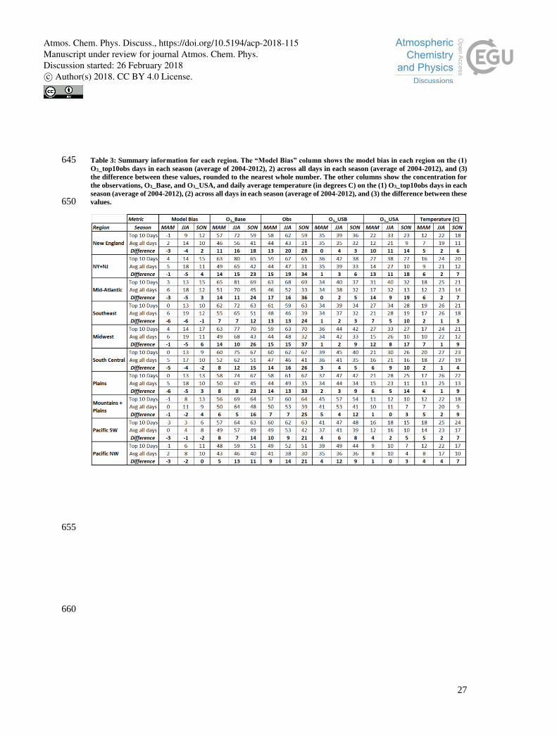
Table 3: Summary information for each region. The “Model Bias” column shows the model bias in each region on the (1) 645 O3_top10obs days in each season (average of 2004-2012), 2) across all days in each season (average of 2004-2012), and (3)

the difference between these values, rounded to the nearest whole number. The other columns show the concentration for

the observations, O3_Base, and O3_USA, and daily average temperature (in degrees C) on the (1) O3_top10obs days in each

season (average of 2004-2012), (2) across all days in each season (average of 2004-2012), and (3) the difference between these

values. 650

655

660


28

Table 4: Summary information for each region. Each column shows the concentration for each background O3 source

influence on the (1) O3_top10obs days in each season (average of 2004-2012), (2) across all days in each season (average of 665 2004-2012), and (3) the difference between these values, rounded to the nearest whole number.

Figure 9: Average 2004-2012 influence of each sensitivity simulation to O3_Base in the (a) Southeast and (b) Mountains and

Plains regions on MDA8 O3_top10obs_JJA days (red) versus averaged across all days (blue). Error bars show the 670 concentration on the lowest versus highest year for each sensitivity simulation in each region.


29

Figure 10: Average yearly MDA8 O3_top10obs_JJA concentrations for observations (divided by 2 to fit on the same axes;

blue dashed line), O3_Base (divided by 2; blue solid line), O3_USB (red), O3_USA (black), O3_NAT (green) MDA8, and daily 675 average temperature (in degrees C; light blue) in the (a) Southeast and (b) Mountains and Plains regions.

Table 5: Change in MDA8 O3 concentrations from 2004-2006 to 2010-2012 on O3_top10obs_JJA days in the observations,

O3_Base, O3_USB, and O3_USA.

Obs O3_Base O3_USB O3_USA

New England -6 -4 6 -10

NY+NJ -2 -4 3 -7

Mid-Atlantic 0 -3 4 -7

Southeast -4 -5 2 -7

Midwest -2 -4 2 -6

South Central -6 -2 5 -7

Plains -1 -2 4 -5

Mountains + Plains -4 -1 1 -2

Pacific SW -3 -4 0 -4

Pacific NW -7 -5 -4 -1

Average -3 -3 2 -6


30

680

Figure 11: Monthly average MDA8 O3_USB (a, b), O3_BVOC (c, d), and O3_SNOx (e, f) concentrations in the Southeast (a,

c, e) and Mountains and Plains (b, d, f) regions.


31

Figure 12: Anomaly on the MDA8 O3_top10obs_JJA days relative to the 2004-2012 average in the Southeast (a, c) and in 685 the Mountains and Plains (b, d) regions. Panels (a) and (b) show the observations, O3_Base, O3_USB, O3_USA, and

temperature (in degrees C). Panels (c) and (d) show O3_BVOC, O3_SNOx, O3_NALNOx, O3_BB, O3_ICT+CH4, and

O3_CA+MX.

Figure 13: Range in magnitude of the MDA8 O3_top10obs for each year shown as vertical lines in the observations (black), 690 O3_Base (blue), and O3_USB (red) in the (a, c) Southeast and (b, d) Mountains and Plains regions. (a, b) show the range on

of O3_top10obs days during each year between 2004-2012. (c, d) show the range of the O3_top10obs days after averaging

over three consecutive years. The solid dots show the 4th highest MDA8 O3 day for each simulation (a, b) and the annual 4th

highest MDA8 O3 day averaged over three consecutive years.

695


Date post:	01-Jul-2018
Category:	Documents
Upload:	vulien
View:	215 times
Download:	0 times

Average versus high s urface ozone levels over the ... · Chem global chemistry ... surfa ce O 3...

Documents