Averaged Stokes polarimetry applied to evaluate retardance and flicker in PA-LCoS devices
Francisco J. Martínez,1,2 Andrés Márquez,1,2,* Sergi Gallego,1,2 Manuel Ortuño,1,2 Jorge Francés,1,2 Augusto Beléndez,1,2 and Inmaculada Pascual2,3
1Dept. de Física, Ing. de Sistemas y Teoría de la Señal, Univ. de Alicante, P.O. Box 99, E-03080, Alicante, Spain 2I.U. Física Aplicada a las Ciencias y las Tecnologías Univ. de Alicante, P.O. Box 99, E-03080, Alicante, Spain
3Dept. de Óptica, Farmacología y Anatomía, Univ. de Alicante, P.O. Box 99, E-03080, Alicante, Spain *[email protected]
Abstract: Recently we proposed a novel polarimetric method, based on Stokes polarimetry, enabling the characterization of the linear retardance and its flicker amplitude in electro-optic devices behaving as variable linear retarders. In this work we apply extensively the technique to parallel-aligned liquid crystal on silicon devices (PA-LCoS) under the most typical working conditions. As a previous step we provide some experimental analysis to delimitate the robustness of the technique dealing with its repeatability and its reproducibility. Then we analyze the dependencies of retardance and flicker for different digital sequence formats and for a wide variety of working geometries.
1. J. Turunen and F. Wyrowski, eds., Diffractive Optics for Industrial and Commercial Applications (Akademie Verlag, 1997).
2. H. J. Coufal, D. Psaltis, and B. T. Sincerbox, eds., Holographic Data Storage, (Springer-Verlag, 2000). 3. W. Osten, C. Kohler, and J. Liesener, “Evaluation and application of spatial light modulators for optical
metrology,” Opt. Pura Apl. 38, 71–81 (2005). 4. M. A. F. Roelens, S. Frisken, J. A. Bolger, D. Abakoumov, G. Baxter, S. Poole, and B. J. Eggleton, “Dispersion
trimming in a reconfigurable wavelength selective switch,” J. Lightwave Technol. 26(1), 73–78 (2008). 5. M. Salsi, C. Koebele, D. Sperti, P. Tran, H. Mardoyan, P. Brindel, S. Bigo, A. Boutin, F. Verluise, P. Sillard, M.
Bigot-Astruc, L. Provost, and G. Charlet, “Mode-division multiplexing of 2 100 Gb/s channels using an LCOS-based spatial modulator,” J. Lightwave Technol. 30(4), 618–623 (2012).
6. M. A. Solís-Prosser, A. Arias, J. J. M. Varga, L. Rebón, S. Ledesma, C. Iemmi, and L. Neves, “Preparing arbitrary pure states of spatial qudits with a single phase-only spatial light modulator,” Opt. Lett. 38(22), 4762–4765 (2013).
7. S. T. Wu and D. K. Yang, Reflective Liquid Crystal Displays (John Wiley, 2005). 8. N. Collings, T. Davey, J. Christmas, D. Chu, and B. Crossland, “The applications and technology of phase-only
liquid crystal on silicon devices,” J. Display Technol. 7(3), 112–119 (2011). 9. J. E. Wolfe and R. A. Chipman, “Polarimetric characterization of liquid-crystal-on-silicon panels,” Appl. Opt.
45(8), 1688–1703 (2006). 10. A. Hermerschmidt, S. Osten, S. Krüger, and T. Blümel, “Wave front generation using a phase-only modulating
liquid-crystal-based micro-display with HDTV resolution,” Proc. SPIE 6584, 65840E (2007). 11. J. R. Moore, N. Collings, W. A. Crossland, A. B. Davey, M. Evans, A. M. Jeziorska, M. Komarčević, R. J.
Parker, T. D. Wilkinson, and H. Xu, “The silicon backplane design for an LCOS polarization-insensitive phase hologram SLM,” IEEE Photon. Technol. Lett. 20(1), 60–62 (2008).
12. I. Moreno, A. Lizana, A. Márquez, C. Iemmi, E. Fernández, J. Campos, and M. J. Yzuel, “Time fluctuations of the phase modulation in a liquid crystal on silicon display: characterization and effects in diffractive optics,” Opt. Express 16(21), 16711–16722 (2008).
13. A. Lizana, I. Moreno, A. Márquez, E. Also, C. Iemmi, J. Campos, and M. J. Yzuel, “Influence of the temporal fluctuations phenomena on the ECB LCoS performance,” Proc. SPIE 7442, 74420G (2009).
14. J. García-Márquez, V. López, A. González-Vega, and E. Noé, “Flicker minimization in an LCoS spatial light modulator,” Opt. Express 20(8), 8431–8441 (2012).
#211179 - $15.00 USD Received 30 Apr 2014; revised 29 May 2014; accepted 1 Jun 2014; published 11 Jun 2014(C) 2014 OSA 16 June 2014 | Vol. 22, No. 12 | DOI:10.1364/OE.22.015064 | OPTICS EXPRESS 15064
15. G. Lazarev, A. Hermerschmidt, S. Krüger, and S. Osten, “LCOS spatial light modulators: trends and applications,” in Optical Imaging and Metrology: Advanced Technologies, W. Osten and N. Reingand, eds. (John Wiley, 2012).
16. F. J. Martínez, A. Márquez, S. Gallego, M. Ortuño, J. Francés, A. Beléndez, and I. Pascual, “Electrical dependencies of optical modulation capabilities in digitally addressed parallel aligned LCoS devices,” Opt. Eng. (accepted for publication).
17. A. Márquez, F. J. Martínez, S. Gallego, M. Ortuño, J. Francés, A. Beléndez, and I. Pascual, “Classical polarimetric method revisited to analyse the modulation capabilities of parallel aligned liquid crystal on silicon displays,” Proc. SPIE 8498, 84980L (2012).
18. F. J. Martínez, A. Márquez, S. Gallego, J. Francés, and I. Pascual, “Extended linear polarimeter to measure retardance and flicker: application to liquid crystal on silicon devices in two working geometries,” Opt. Eng. 53, 014105 (2014).
19. C. Ramirez, B. Karakus, A. Lizana, and J. Campos, “Polarimetric method for liquid crystal displays characterization in presence of phase fluctuations,” Opt. Express 21(3), 3182–3192 (2013).
20. F. J. Martínez, A. Márquez, S. Gallego, J. Francés, I. Pascual, and A. Beléndez, “Retardance and flicker modeling and characterization of electro-optic linear retarders by averaged Stokes polarimetry,” Opt. Lett. 39(4), 1011–1014 (2014).
21. A. Lizana, N. Martín, M. Estapé, E. Fernández, I. Moreno, A. Márquez, C. Iemmi, J. Campos, and M. J. Yzuel, “Influence of the incident angle in the performance of liquid crystal on silicon displays,” Opt. Express 17(10), 8491–8505 (2009).
22. G. Goldstein, Polarized Light (Marcel Dekker, 2003). 23. C. Flueraru, S. Latoui, J. Besse, and P. Legendre, “Error analysis of a rotating quarter-wave plate Stokes’
polarimeter,” IEEE Trans. Instrum. Meas. 57(4), 731–735 (2008). 24. T. G. Brown and Q. Zhan, “Introduction: unconventional polarization states of light,” Opt. Express 18, 10775–
10776 (2010).
1. Introduction
In recent years liquid crystal on silicon (LCoS) displays have become the most attractive microdisplays for all sort of spatial light modulation applications, like in diffractive optics [1], optical storage [2], optical metrology [3], reconfigurable interconnects [4,5], or quantum optical computing [6], due to their very high spatial resolution and very high light efficiency [7,8]. Among the different LCoS technologies, parallel aligned LCoS (PA-LCoS) are especially interesting since they allow easy operation as phase-only devices without coupled amplitude modulation. From a modeling point of view PA-LCoS displays can be assimilated to linear variable retarders [7,8], then the magnitude of interest to characterize these devices is their linear retardance.
It is known that LCoS and more specifically PA-LCoS exhibit some flicker or fluctuations [9–14]. This is generally true in digital backplane devices due to the pulsed digital signal addressed [10,11,15,16]. Typical methods used to characterize linear variable retarders may provide erroneous results [17,18] since they typically assume that the birefringence in the waveplate has a constant value, no fluctuations, during the measurement process. Furthermore, the amplitude of the retardance fluctuation becomes a magnitude of interest for a more accurate characterization and modeling of the device under test. Recently appropriate techniques to obtain both retardance and flicker values have been demonstrated by our group [18] and by Ramirez et al. [19], based respectively on the classical linear polarimeter and in a combination of linear and circular polarimeters. These are easier techniques to implement, specially the extended linear polarimeter in [18]. However, a more detailed characterization can be obtained by the average Stokes polarimetry method we recently proposed in [20]. This technique in combination with a Mueller matrix based model allows us to predict the response of the device for every gray level and any kind of state of polarization (SOP) at the system entry.
A first parameter to be evaluated in the performance of a digital backplane LCoS is the sequence format addressed. This may affect the number of available quantization levels and also the amount of flicker exhibited by the device [16]. Another important aspect is the working geometry where the LCoS is used: angle of incidence, use of a beam-splitter, may change the retardance dynamic range, linearity in the response [21].
#211179 - $15.00 USD Received 30 Apr 2014; revised 29 May 2014; accepted 1 Jun 2014; published 11 Jun 2014(C) 2014 OSA 16 June 2014 | Vol. 22, No. 12 | DOI:10.1364/OE.22.015064 | OPTICS EXPRESS 15065
In this work we apply the average Stokes polarimetry method for the evaluation of the linear retardance and flicker amplitude in PA-LCoS devices. We present a study about the robustness of the method, focused on reproducibility and repeatability capabilities of the technique. Then, a complete analysis of the performance of the PA-LCoS for a series of different sequence formats addressed and for various working geometries is undertaken.
2. Theory and characterization method
The average Stokes polarimetric technique [20] is based on the Mueller-Stokes formalism [22], which enables to deal both with polarized and with unpolarized light. The approach is valid for the modeling and characterization of linear variable retarders whose linear retardance exhibits instabilities, such as PA-LCoS displays. In principle the Mueller matrix
( )RM Γ of a linear retarder with a retardance value Γ, with its fast axis along the X-axis is
given by,
( )
1 0 0 0
0 1 0 0
0 0 cos sin
0 0 sin cos
RM
Γ = Γ Γ − Γ Γ
(1)
We showed in [20] that a reasonable assumption in the case of PA-LCoS is that temporal evolution of fluctuations ( )tΓ can be approximated by triangular time-dependent profile,
characterized by its average retardance Γ and its fluctuation amplitude a , defined as half the maximum-to-minimum value for the fluctuation. Taking into account this time-dependent linear model we can describe the averaged matrix for the linear retarder as:
( ) ( )( ) ( )
1 0 0 0
0 1 0 0( , )
0 0 sin cos sin sin
0 0 sin sin sin cos
RM aa a a a
a a a a
Γ = Γ Γ − Γ Γ
(2)
This expression provides a more realistic and precise model of the linear retarder, where the average retardance and its fluctuation need to be characterized.
Since PA-LCoS displays are reflective devices, in order to analyze the output SOP, an inversion of the horizontal axis must be considered between the corresponding forward and the backward (right-handed) reference systems, which in the Mueller-Stokes formalism is expressed by the inversion matrix as follows,
1 0 0 0
0 1 0 0
0 0 1 0
0 0 0 1
Inv
= − −
(3)
Then, the averaged reflected SOP outS can be calculated as,
( , )out R inS Inv M a S= ⋅ Γ ⋅ , (4)
where inS corresponds to the input SOP. We may find specific input SOPs which may proof
useful to measure the two parameters in the model, Γ and a [20]. In this sense, if the beam impinging the retarder corresponds to linearly polarized light at + 45° with respect to the X
#211179 - $15.00 USD Received 30 Apr 2014; revised 29 May 2014; accepted 1 Jun 2014; published 11 Jun 2014(C) 2014 OSA 16 June 2014 | Vol. 22, No. 12 | DOI:10.1364/OE.22.015064 | OPTICS EXPRESS 15066
axis, i.e. (S0 = 1, S1 = 0, S2 = 1, S3 = 0), the average SOP and the degree of polarization, DoP, at the output of the device will be expressed as follows:
( )( )
1
0
sin cos
sin sin
outSa a
a a
= − Γ Γ
(5)
( )sinDoP a a= (6)
We note that the output S1 component is zero independently of the retardance and its fluctuation amplitude. The expression for DoP is also straightforward and is directly related to the fluctuation amplitude. Equations (5) and (6) can be used to measure both the average
retardance value Γ and its fluctuation amplitude a . This can be easily accomplished using Eq. (6) to obtain the fluctuation amplitude a , and the ratio between the 3rd and 4rth Stokes
vector components, i.e. 3 2 ( )S S tg− = Γ , to obtain Γ .
3. Calibration and robustness results
3.1 Calibration and comparison with instantaneous values from the linear polarimeter
The model and the accompanying calibration technique may be applied to any device which can be modeled as a variable waveplate retarder. We apply the technique to a commercial PA-LCoS display, model PLUTO distributed by the company HOLOEYE. It is a nematic liquid crystal filled, with 1920x1080 pixels and 0.7” diagonal, and digitally addressed. By means of a RS-232 interface and its corresponding provided software, we can configure the modulator for different applications and wavelengths. Besides, different pulse width modulation (PWM) addressing schemes (digital addressing sequences) can be generated by the driver electronics [10,16]. We have selected two electrical sequences exhibiting a clearly different scale of fluctuations, whose configuration files are provided with the software. They correspond to the configurations labeled as “18-6 633 2pi linear” and “5-5 633 2pi linear”.
The averaged polarimetric measurements have been obtained with a Stokes polarimeter, model PAX5710VIS-T distributed by the company THORLABS. This is a rotating waveplate-based polarimeter, which belongs to time-division mode polarimeters [23]. Its software allows different time interval options so as to obtain an averaged signal. When enough rotations are considered, and if the periods of fluctuation and half-rotation are not multiple, then for each angular position of the rotating waveplate the amount of samples collected is representative of the time-varying SOP generated by the fluctuations in the device. The polarimeter averaging time considered in the paper, 600 ms, is much larger than actually needed to obtain fully stable and repeatable SOP measurements. Note that the time period (frequency) for the fluctuations in our PA-LCoS device is 8.66 ms (120 Hz).
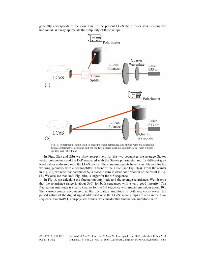
In Figs. 1(a) and 1(b) we show respectively the diagrams for the characterization setup associated with the two generic working geometries used with the PA-LCoS display, that is, with and without a beam-splitter in front. The unexpanded beam from a laser (He-Ne laser at 633 nm in this work) incides onto a polarizer with its transmission axis at + 45° with respect to the laboratory vertical (X-axis for the right-handed system used in this work). When using polarized laser light an additional waveplate must be inserted before the polarizer to secure that enough light traverses the polarizer. In Fig. 1(a) light impinges perpendicularly to the LCoS and a non-polarizing cube beam-splitter (model 10BC16NP.4, from Newport, in this work) separates the input and the reflected beam, which eventually is detected by the polarimeter head. Thus, strictly speaking the characterization corresponds to the combination of LCoS and cube. In Fig. 1(b) the polarimeter head measures directly the reflected beam from the LCoS. We note that the director axis (extraordinary axis) in nematic based LCoS
#211179 - $15.00 USD Received 30 Apr 2014; revised 29 May 2014; accepted 1 Jun 2014; published 11 Jun 2014(C) 2014 OSA 16 June 2014 | Vol. 22, No. 12 | DOI:10.1364/OE.22.015064 | OPTICS EXPRESS 15067
generally corresponds to the slow axis. In the present LCoS the director axis is along the horizontal. We may appreciate the simplicity of these setups.
Laser633 nm
LCoS BeamSplitter
LinearPolarizer
QuarterWaveplate
Polarimeter
Laser633 nm
LCoS
LinearPolarizer
QuarterWaveplate
Polarimeter
(a)
(b)
Fig. 1. Experimental setup used to measure linear retardance and flicker with the averaging Stokes polarimetric technique and for the two generic working geometries: (a) with a beam-splitter, and (b) without.
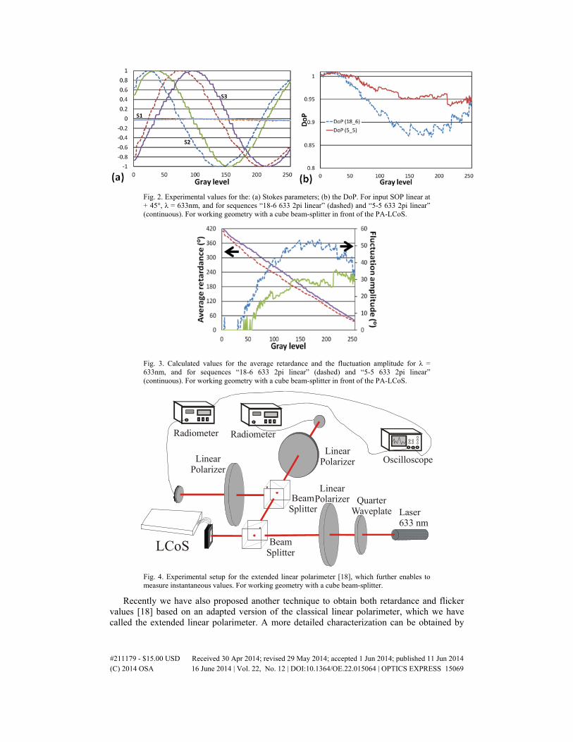
In Figs. 2(a) and 2(b) we show respectively for the two sequences the average Stokes vector components and the DoP measured with the Stokes polarimeter and for different gray level values addressed onto the LCoS device. These measurements have been obtained for the working geometry with a beam-splitter in front of the LCoS (see Fig. 1(a)). From the results in Fig. 2(a) we note that parameter S1 is close to zero in clear confirmation of the result in Eq. (5). We also see that DoP, Fig. 2(b), is larger for the 5-5 sequence.
In Fig. 3, we calculate the fluctuation amplitude and the average retardance. We observe that the retardance range is about 360° for both sequences with a very good linearity. The fluctuation amplitude is clearly smaller for the 5-5 sequence with maximum values about 30°. The various jumps encountered in the fluctuation amplitude in both sequences reveal the pulsed nature of the digital signal addressed onto the LCoS: more jumps are seen in the 18-6 sequence. For DoP>1, non-physical values, we consider that fluctuation amplitude is 0°.
#211179 - $15.00 USD Received 30 Apr 2014; revised 29 May 2014; accepted 1 Jun 2014; published 11 Jun 2014(C) 2014 OSA 16 June 2014 | Vol. 22, No. 12 | DOI:10.1364/OE.22.015064 | OPTICS EXPRESS 15068
Fig. 2. Experimental values for the: (a) Stokes parameters; (b) the DoP. For input SOP linear at + 45°, λ = 633nm, and for sequences “18-6 633 2pi linear” (dashed) and “5-5 633 2pi linear” (continuous). For working geometry with a cube beam-splitter in front of the PA-LCoS.
Fig. 3. Calculated values for the average retardance and the fluctuation amplitude for λ = 633nm, and for sequences “18-6 633 2pi linear” (dashed) and “5-5 633 2pi linear” (continuous). For working geometry with a cube beam-splitter in front of the PA-LCoS.
Laser633 nm
LinearPolarizer
Radiometer
LinearPolarizer
BeamSplitter
LCoS BeamSplitter
LinearPolarizer Quarter
Waveplate
Radiometer
Oscilloscope
Fig. 4. Experimental setup for the extended linear polarimeter [18], which further enables to measure instantaneous values. For working geometry with a cube beam-splitter.
Recently we have also proposed another technique to obtain both retardance and flicker values [18] based on an adapted version of the classical linear polarimeter, which we have called the extended linear polarimeter. A more detailed characterization can be obtained by
#211179 - $15.00 USD Received 30 Apr 2014; revised 29 May 2014; accepted 1 Jun 2014; published 11 Jun 2014(C) 2014 OSA 16 June 2014 | Vol. 22, No. 12 | DOI:10.1364/OE.22.015064 | OPTICS EXPRESS 15069
the average Stokes polarimetry, however the extended linear polarimeter can be more widely applied by any lab since only two linear polarizers are needed. At this moment we want to take advantage that this setup also enables the measurement of the instantaneous values for the retardance as we showed in [18]. We want to compare the average Stokes polarimetry results against the values calculated from the instantaneous values of retardance.
In Fig. 4 we show the experimental setup corresponding to the linear polarimeter [18], where the necessary input and output linear polarizers to be used in parallel or crossed configuration can be seen. The working geometry considered in the figure is the perpendicular one where a non-polarizing cube beam splitter is used to separate the incident and reflected beams. There is a second one to enable amplitude division of the reflected beam so that crossed and parallel intensity can be measured simultaneously. Instantaneous measurements can be obtained by connecting the two radiometers to the two channels of an oscilloscope.
Table 1. Average retardance and fluctuation amplitude obtained with the average Stokes polarimetric method (columns 3 and 4) and with the instantaneous measurements
In Table 1 we show the values for the average retardance and its fluctuation amplitude obtained by means of average Stokes polarimetry (columns 3 and 4), plotted in Fig. 3, against the corresponding values calculated from the instantaneous values of retardance (columns 5 and 6), and measured with the setup in Fig. 4. The results have been obtained for the two sequences and for a series of applied gray levels sampling the whole voltage range. There exists a good agreement between the average Stokes polarimetry method results and the ones related with instantaneous values measurement. This provides an alternative validation of the average Stokes polarimetry characterization technique proposed, which complements the validation already presented in [20], which was based on its capability to predict the Stokes vector for the SOP reflected by the LCoS for arbitrary input SOPs.
3.2 Robustness analysis
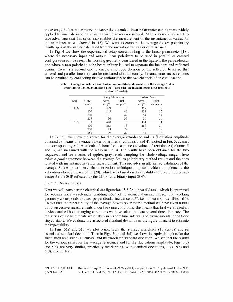
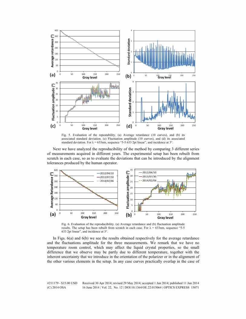
Next we will consider the electrical configuration “5-5 2pi linear 633nm”, which is optimized for 633nm laser wavelength, enabling 360° of retardance dynamic range. The working geometry corresponds to quasi-perpendicular incidence at 3°, i.e. no beam-splitter (Fig. 1(b)). To evaluate the repeatability of the average Stokes polarimetric method we have taken a total of 10 successive measurements under the same conditions: this means that first we aligned all devices and without changing conditions we have taken the data several times in a row. The ten series of measurements were taken in a short time interval and environmental conditions stayed stable. We evaluate the associated standard deviation as the figure of merit to estimate the repeatability.
In Figs. 5(a) and 5(b) we plot respectively the average retardance (10 curves) and its associated standard deviation. Then in Figs. 5(c) and 5(d) we show the equivalent plots for the fluctuation amplitude (10 curves) and its associated standard deviation. We see that the results for the various series for the average retardance and for the fluctuations amplitude, Figs. 5(a) and 5(c), are very similar, practically overlapping, with standard deviations, Figs. 5(b) and 5(d), around 1-2°.
#211179 - $15.00 USD Received 30 Apr 2014; revised 29 May 2014; accepted 1 Jun 2014; published 11 Jun 2014(C) 2014 OSA 16 June 2014 | Vol. 22, No. 12 | DOI:10.1364/OE.22.015064 | OPTICS EXPRESS 15070
Fig. 5. Evaluation of the repeatability. (a) Average retardance (10 curves), and (b) its associated standard deviation. (c) Fluctuation amplitude (10 curves), and (d) its associated standard deviation. For λ = 633nm, sequence “5-5 633 2pi linear”, and incidence at 3°.
Next we have analyzed the reproducibility of the method by comparing 3 different series of measurements acquired in different years. The experimental setup has been rebuilt from scratch in each case, so as to evaluate the deviations that can be introduced by the alignment tolerances produced by the human operator.
Fig. 6. Evaluation of the reproducibility. (a) Average retardance and (b) fluctuation amplitude results. The setup has been rebuilt from scratch in each case. For λ = 633nm, sequence “5-5 633 2pi linear”, and incidence at 3°.
In Figs. 6(a) and 6(b) we see the results obtained respectively for the average retardance and the fluctuations amplitude for the three measurements. We remark that we have no temperature room control, which may affect the liquid crystal properties, so the small difference that we observe may be partly due to different temperature, together with the inherent uncertainty that we introduce in the orientation of the polarizer or in the alignment of the other various elements in the setup. In any case curves practically overlap in the case of
#211179 - $15.00 USD Received 30 Apr 2014; revised 29 May 2014; accepted 1 Jun 2014; published 11 Jun 2014(C) 2014 OSA 16 June 2014 | Vol. 22, No. 12 | DOI:10.1364/OE.22.015064 | OPTICS EXPRESS 15071
average retardance, Fig. 6(a), and are also quite similar in the case of the fluctuations amplitude, Fig. 6(b).
The results in Figs. 5 and 6 provide an overview of the robustness of the method, which is very high for the average retardance measurements, and still quite remarkable in the case of the fluctuations amplitude measurements.
4. Evaluation of sequence formats and working geometries
Once the technique has been presented and its robustness has been analyzed, next we consider the characterization of the PA-LCoS for the two electrical sequences and in three typical working geometries [21]: perpendicular incidence with a beam-splitter in front (see Fig. 1(a)), quasi-perpendicular incidence at about 3°, and right-angle (45°) incidence. In the two latter geometries no beam-splitter is necessary in front of the LCoS, see Fig. 1(b). We have added a fourth characterization geometry corresponding to the setup used in previous Fig. 4 for the instantaneous measurements, where two beam-splitters are considered. In this case the polarimeter is located in transmission after the second beam-splitter. We want to estimate the influence of the insertion of the second beam-splitter. This is used not only for the instantaneous measurements but also to ease the measurements acquisition in the extended linear polarimeter, proposed in [18].
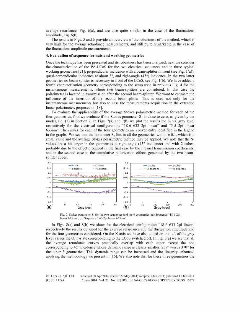
To evaluate the applicability of the average Stokes polarimetric method for each of the four geometries, first we evaluate if the Stokes parameter S1 is close to zero, as given by the model, Eq. (5) in Section 2. In Figs. 7(a) and 7(b) we plot the results for S1 vs. gray level respectively for the electrical configurations “18-6 633 2pi linear” and “5-5 2pi linear 633nm”. The curves for each of the four geometries are conveniently identified in the legend in the graphs. We see that the parameter S1 lies in all the geometries within ± 0.1, which is a small value and the average Stokes polarimetric method may be applied. We note that the S1 values are a bit larger in the geometries at right-angle (45° incidence) and with 2 cubes, probably due to the effect produced in the first case by the Fresnel transmission coefficients, and in the second case to the cumulative polarization effects generated by the two beam-splitter cubes.
Fig. 7. Stokes parameter S1 for the two sequences and the 4 geometries: (a) Sequence “18-6 2pi linear 633nm”, (b) Sequence “5-5 2pi linear 633nm”.
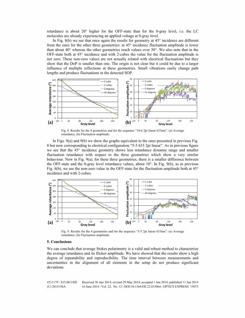
In Figs. 8(a) and 8(b) we show for the electrical configuration “18-6 633 2pi linear” respectively the results obtained for the average retardance and the fluctuation amplitude and for the four geometries considered. On the X-axis we have also added on the left of the gray level values the OFF-state corresponding to the LCoS switched off. In Fig. 8(a) we see that all the average retardance curves practically overlap with each other except the one corresponding to 45° incidence whose dynamic range is clearly smaller: 257° versus 370° for the other 3 geometries. This dynamic range can be increased and the linearity enhanced applying the methodology we present in [16]. We also note that for these three geometries the
#211179 - $15.00 USD Received 30 Apr 2014; revised 29 May 2014; accepted 1 Jun 2014; published 11 Jun 2014(C) 2014 OSA 16 June 2014 | Vol. 22, No. 12 | DOI:10.1364/OE.22.015064 | OPTICS EXPRESS 15072
retardance is about 20° higher for the OFF-state than for the 0-gray level, i.e. the LC molecules are already experiencing an applied voltage at 0-gray level.
In Fig. 8(b) we see that once again the results for geometry at 45° incidence are different from the ones for the other three geometries: at 45° incidence fluctuation amplitude is lower than about 40° whereas the other geometries reach values over 50°. We also note that in the OFF-state both at 45° incidence and with 2-cubes the value for the fluctuation amplitude is not zero. These non-zero values are not actually related with electrical fluctuations but they show that the DoP is smaller than one. The origin is not clear but it could be due to a larger influence of multiple reflections at these geometries. Small vibrations easily change path lengths and produce fluctuations in the detected SOP.
Fig. 8. Results for the 4 geometries and for the sequence “18-6 2pi linear 633nm”: (a) Average retardance, (b) Fluctuation amplitude.
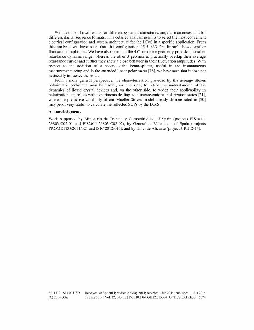
In Figs. 9(a) and 9(b) we show the graphs equivalent to the ones presented in previous Fig. 8 but now corresponding to electrical configuration “5-5 633 2pi linear”. As in previous figure we see that the 45° incidence geometry shows less retardance dynamic range and smaller fluctuation retardance with respect to the three geometries which show a very similar behaviour. Now in Fig. 9(a), for these three geometries, there is a smaller difference between the OFF-state and the 0-gray level retardance values, about 10°. In Fig. 9(b), as in previous Fig. 8(b), we see the non-zero value in the OFF-state for the fluctuation amplitude both at 45° incidence and with 2-cubes.
Fig. 9. Results for the 4 geometries and for the sequence “5-5 2pi linear 633nm”: (a) Average retardance, (b) Fluctuation amplitude.
5. Conclusions
We can conclude that average Stokes polarimetry is a valid and robust method to characterize the average retardance and its flicker amplitude. We have showed that the results show a high degree of repeatability and reproducibility. The time interval between measurements and uncertainties in the alignment of all elements in the setup do not produce significant deviations.
#211179 - $15.00 USD Received 30 Apr 2014; revised 29 May 2014; accepted 1 Jun 2014; published 11 Jun 2014(C) 2014 OSA 16 June 2014 | Vol. 22, No. 12 | DOI:10.1364/OE.22.015064 | OPTICS EXPRESS 15073
We have also shown results for different system architectures, angular incidences, and for different digital sequence formats. This detailed analysis permits to select the most convenient electrical configuration and system architecture for the LCoS in a specific application. From this analysis we have seen that the configuration “5-5 633 2pi linear” shows smaller fluctuation amplitudes. We have also seen that the 45° incidence geometry provides a smaller retardance dynamic range, whereas the other 3 geometries practically overlap their average retardance curves and further they show a close behavior in their fluctuation amplitudes. With respect to the addition of a second cube beam-splitter, useful in the instantaneous measurements setup and in the extended linear polarimeter [18], we have seen that it does not noticeably influence the results.
From a more general perspective, the characterization provided by the average Stokes polarimetric technique may be useful, on one side, to refine the understanding of the dynamics of liquid crystal devices and, on the other side, to widen their applicability in polarization control, as with experiments dealing with unconventional polarization states [24], where the predictive capability of our Mueller-Stokes model already demonstrated in [20] may proof very useful to calculate the reflected SOPs by the LCoS.
Acknowledgments
Work supported by Ministerio de Trabajo y Competitividad of Spain (projects FIS2011-29803-C02-01 and FIS2011-29803-C02-02), by Generalitat Valenciana of Spain (projects PROMETEO/2011/021 and ISIC/2012/013), and by Univ. de Alicante (project GRE12-14).
#211179 - $15.00 USD Received 30 Apr 2014; revised 29 May 2014; accepted 1 Jun 2014; published 11 Jun 2014(C) 2014 OSA 16 June 2014 | Vol. 22, No. 12 | DOI:10.1364/OE.22.015064 | OPTICS EXPRESS 15074