77
Mathematics for Public Policy Avidit Acharya September 23, 2010

Mathematics for Public Policy
Avidit Acharya
September 23, 2010
Contents
1 Introduction 4
1.1 Mathematical Statements . . . . . . . . . . . . . . . . . . . . . . . . 4
1.2 Proving Mathematical Statements . . . . . . . . . . . . . . . . . . . . 6
1.3 Numbers and Shorthands . . . . . . . . . . . . . . . . . . . . . . . . . 7
2 Preliminaries 8
2.1 Sets, Relations and Functions . . . . . . . . . . . . . . . . . . . . . . 8
2.2 Economic Preference Theory . . . . . . . . . . . . . . . . . . . . . . . 10
2.3 Application: Social Choice Theory . . . . . . . . . . . . . . . . . . . 12
3 Differential Calculus 15
3.1 Limits, Continuity and the Derivative . . . . . . . . . . . . . . . . . . 15
3.2 Properties of the Derivative . . . . . . . . . . . . . . . . . . . . . . . 18
3.3 Some Matrix Algebra . . . . . . . . . . . . . . . . . . . . . . . . . . . 19
3.4 The Derivative in Multiple Dimensions . . . . . . . . . . . . . . . . . 21
4 Real Analysis 24
4.1 Intermediate Value Theorem . . . . . . . . . . . . . . . . . . . . . . . 25
4.2 Heine-Borel Theorem . . . . . . . . . . . . . . . . . . . . . . . . . . . 25
4.3 Weierstrass Theorem . . . . . . . . . . . . . . . . . . . . . . . . . . . 26
4.4 Mean Value Theorem . . . . . . . . . . . . . . . . . . . . . . . . . . . 27
4.5 L’Hopital’s Rule . . . . . . . . . . . . . . . . . . . . . . . . . . . . . . 29
4.6 Implicit Function Theorem . . . . . . . . . . . . . . . . . . . . . . . . 30
4.7 Inverse Function Theorem . . . . . . . . . . . . . . . . . . . . . . . . 32
4.8 Application: The Swan-Solow Model . . . . . . . . . . . . . . . . . . 34
1
5 Linear Algebra 37
5.1 Cauchy-Schwartz Inequality . . . . . . . . . . . . . . . . . . . . . . . 37
5.2 The Rank of a Matrix . . . . . . . . . . . . . . . . . . . . . . . . . . 37
5.3 The Determinant . . . . . . . . . . . . . . . . . . . . . . . . . . . . . 40
5.4 Cramer’s Rule . . . . . . . . . . . . . . . . . . . . . . . . . . . . . . . 41
5.5 The Inverse of a Matrix . . . . . . . . . . . . . . . . . . . . . . . . . 42
5.6 Eigenvectors and eigenvalues . . . . . . . . . . . . . . . . . . . . . . . 43
5.7 Application: Central Planning . . . . . . . . . . . . . . . . . . . . . . 44
6 Integration 48
6.1 Upper and Lower Sums . . . . . . . . . . . . . . . . . . . . . . . . . . 48
6.2 Integrability of Continuous Functions . . . . . . . . . . . . . . . . . . 49
6.3 Properties of the Integral . . . . . . . . . . . . . . . . . . . . . . . . . 50
6.4 The Fundamental Theorem of Calculus . . . . . . . . . . . . . . . . . 51
6.5 Integration by Parts . . . . . . . . . . . . . . . . . . . . . . . . . . . 52
6.6 Fubini’s Theorem . . . . . . . . . . . . . . . . . . . . . . . . . . . . . 52
6.7 The Change of Variables . . . . . . . . . . . . . . . . . . . . . . . . . 53
6.8 Improper Integrals . . . . . . . . . . . . . . . . . . . . . . . . . . . . 54
6.9 Taylor’s Theorem . . . . . . . . . . . . . . . . . . . . . . . . . . . . . 54
7 Optimization 57
7.1 Optimization in R . . . . . . . . . . . . . . . . . . . . . . . . . . . . . 57
7.2 Optimization in Rn . . . . . . . . . . . . . . . . . . . . . . . . . . . . 58
7.3 Lagrange’s Theorem . . . . . . . . . . . . . . . . . . . . . . . . . . . 61
7.4 The Karush-Kuhn-Tucker Theorem . . . . . . . . . . . . . . . . . . . 63
7.5 Proof of Lagrange’s Theorem . . . . . . . . . . . . . . . . . . . . . . 66
7.6 Second Order Conditions . . . . . . . . . . . . . . . . . . . . . . . . . 68
7.7 The Kuhn-Tucker Theorem . . . . . . . . . . . . . . . . . . . . . . . 70
7.8 Envelope Theorem . . . . . . . . . . . . . . . . . . . . . . . . . . . . 71
7.9 Application: The Agricultural Household . . . . . . . . . . . . . . . . 73
2

Disclaimer: I am not claiming originality for these notes. Almost all of the theorems
and proofs have been taken from various other sources, and in some cases (especially
where the exposition is particularly elegant) they have been copied verbatim from
these sources. I compiled these notes only to organize my lectures in teaching math-
ematics in the to D-track MPA students at the Woodrow Wilson School, Princeton
University. I taught this class for three consecutive summers, 2008-2010.
While it is impossible for me to list all of the sources for this material, I list
some of the major sources as follows. The proof of the Muller-Satterthwaite The-
orem in Section 2.3 is the proof that appears in Philip Reny’s “Arrow’s Theorem
and the Gibbard Satterthwaite Theorem: A Unified Approach,” Economics Letters,
70, 2001, 91-105. Most of Section 3, almost all of Section 4, and Sections 6.1-6.8
are transplanted here from Richard Beals’s Analysis: An Introduction, Cambridge:
Cambridge University Press, 2004 – a beautiful book that I used as an undergrad-
uate. The exposition on the implicit function theorem in Section 4.6 was inspired
by Steven Krantz and Harold Parks’s Implicit Function Theorem: History, Theory
and Applications, Boston: Birkhauser, 2002. The continuous-time Solow model that
appears in Section 4.8 is taken from Robert Barro and Xavier Sala-i-Martin’s Eco-
nomic Growth, Camrbridge, MA: The MIT Press, 1995. Section 5 on Linear Algebra
is taken from Serge Lang’s Introduction to Linear Algebra, New York: Springer-
Verlag, 1987, and Rangarajan Sundaram’s A First Course in Optimization Theory,
Cambridge: Cambridge University Press, 1996. Sundaram’s book is also the source
for the part on Taylor’s theorem in Rn appearing in Section 6.9 and the exposition
on Lagrange’s theorem in Sections 7.3, 7.5 and 7.6. Section 6.9 on Taylor’s theorem
in R is from Serge Lang’s Undergraduate Analysis, New York: Springer-Verlag, 1997.
The remainder of Section 7 with the exception of Section 7.9 is from Geoffrey Jehle
and Philip Reny’s Advanced Microeconomic Theory, Boston: Addison-Wesley, 2001.
Section 7.9 on the Agricultural Household Model is from Pranab Bardhan and Chris
Udry’s Development Microeconomics, Oxford: Oxford University Press, 1999.
Lastly, every year when I teach the course I discover a few more typos, sometimes
even errors. Although this is the latest version of the notes, I am sure that there
are still many typos and errors left. If you discover any, please email them to me at
3

Chapter 1
Introduction
1.1 Mathematical Statements
The table at the bottom of the page lists some common mathematical symbols and
their abbreviations. Mathematical statements in this course will seldom involve
abbreviations or symbols other than the ones listed in the table (except ones that
you surely already know such as =, ≥ etc.). When new symbols arise, I will explain
them. As an example, a typical statement is
∀x ∈ X and ∀y ∈ Y , ∃z ∈ Z s.t. x+ y = z,
which you will read
For every x in the set X and every y in the set Y ,
there is an element z in the set Z such that x plus y equals z.
Thus a mathematical statement is nothing more than a statement in the English
language (or any other language for that matter), where the vocabulary is limited to
Symbol How to read it
∈ “in the set” or “is in the set” depending on context
∃ “there is a(n),”
∀ “for all” or “for every”
s.t. “such that”1
w.l.o.g. “without loss of generality”
4

words like “for all,” “there is,” and “such that.” Our objective will be to determine
which statements are true, and which are not.
In mathematics, no statement is true in an absolute sense. That is, every state-
ment must be derived from other statements. Put another way, the claim that
statement S1 is true is always meaningless. Only claims of the form “S1 is true if S2
and S3 are both true” are meaningful. For the claim to be right, we must be able to
derive S1 when we assume that S2 and S3 are true. At the end of the day, something
must be assumed. We cannot derive mathematical statements from nothing.
In light of that, it is useful to note the difference between “if” and “only if.” S1
if S2 means that you can derive S1 from S2, but it may not be the case that you
can derive S2 from S1. On the other hand, S1 only if S2 means that you can derive
S2 from S1 but that you may not be able to derive S1 from S2. S1 if and only if S2
means that S1 can be derived from S2 and S2 can be derived from S1. When this
happens, S1 and S2 are equivalent: one statement does not say any more or any
less than the other statement. Think about that.
Every mathematical statement has a negation. The negation of statement S1 is
written ¬S1. For example, you can negate the statement
“Every left-handed man in Princeton has a beard,”
by presenting a left-handed man in Princeton who does not have a beard. Sometimes
in the policy world we meet people who would try to negate this statement by
presenting a right-handed man in Princeton who has a beard. (You should not take
any policy advice from such people.) Another common error is to present a beard-
less left-handed woman in Princeton. You may find it hard to believe that people
make these errors, but trust me you will encounter them in life. The negation of the
above statement is only the statement
“There is a left-handed man in Princeton who does not have a beard.”
The statement “S1 is true if S2 is true” is equivalent to the statement “¬S2 is true
if ¬S1 is true,” or “S2 is not true if S1 is not true.” The latter two statements are
the contrapositive of the first statement. A statement is always equivalent to its
contrapositive.
5

A statement is not equivalent to its converse. The converse of the statement
“S1 is true if S2 is true” is the statement “S2 is true if S1 is true.” To see this, let
S1 be the statement “U2 rocks,” and S2 be the statement “All Irish bands rock.”
Mathematicians organize their lives by assigning different names for similar things.
Lemma, Claim, Proposition and Theorem all refer to statements that are to be
proven, while Axiom, Postulate and Assumption refer to statements that are as-
sumed to be true. A Corollary is an immediate consequence of a Theorem, which is
a statement that is very useful to know. A Lemma is not useful per se, except to
prove a Theorem. Propositions are interesting results that may or may not be useful,
while Claims differ from Propositions in that they are not that interesting. This is
all my own rough understanding of the taxonomy of results, but as you may rightly
think, the lines between these concepts can be very blurry.
1.2 Proving Mathematical Statements
In this course, we will be doing proofs. Often we will prove a statement directly from
a set of other statements. But this may not always be convenient. If we assume that
S1 is true and would like to prove that S2 is true, then one way of doing this is to
begin the proof by assuming that S2 is not true. Then we show that ¬S2 implies
¬S1. But this cannot be, since we assumed S1 is true. Therefore, ¬S2 must be
false, i.e. S2 must be true, and that completes the proof. You may have already
noticed that this is simply proving the statement “S1 implies S2” by proving the
contrapositive. In any case, this kind of proof is called a proof by contradiction.
It is closely related to the method of proof called reductio ad absurdum, which
allows us to conclude that the statement S1 is false if S1 implies a statement S2 and
its negation ¬S2. (Both S2 and ¬S2 cannot simultaneously be true, so S1 must be
false.) I recommend reading the Wikipedia article on reductio ad absurdum.
The third common method of proof is proof by induction. Suppose you wanted
to prove that a sequence of statements S1, S2, S3 ... are all true if S0 is true. If the
sequence never terminates, you have no hope of doing this in your lifetime if you try
to prove each statement one at a time. But there is a shortcut. First you show that
S1 is true if S0 is true. Then you show that for any positive integer k, Sk implies
Sk+1 when S0 is true. That completes the proof. The reason this works is because
6

you can substitute 1 for k, and since you showed S1 is true, S2 must be true. Then
substitute 2 for k, and you get the result that S3 is true, etc. In strong induction
you show that S1 is true. Then you show that for every positive integer k, S1, ..., Skimplies Sk+1. This is similar to induction.
How do you feel about induction?
There are also other methods of proof. You can google search “methods of proof”
to find out what they are if you are so enthusiastic about math camp that you can’t
sit still. The reason I think proofs are important for public policy is that proofs
are simply arguments, and making an argument is an important skill to have in the
policy world.
1.3 Numbers and Shorthands
When I say “number” in this course I always mean a real number (except in some
cases where I mean a positive integer – you will know this by context). The set of
real numbers will be denoted R, which consists of all the numbers you know, except
the imaginary numbers (e.g. 32,−0.73, 0, 19/7, 4π, and e23 are all in R, but 5i is
not). Beyond this, I do not want to go into much detail about what a real number
is. When the symbols ≥, <, ≤, > are used, two numbers are being compared. The
two sides of the equal sign, =, may have numbers or other kinds of objects such as
sets. The context will make that clear. One common shorthand that I will use is
“∀i = 1, 2, 3...” which you will read as “for every positive integer i.”
7

Chapter 2
Preliminaries
2.1 Sets, Relations and Functions
A set is a “well-defined” collection of elements. “Well-defined” means that I can de-
scribe to you what kinds of things are in the set, and you will be able to know exactly
whether something is in the set or not. For example, if I ask you to consider the set
of even numbers, you know exactly whether 591 is in the set or not. Sometimes, we
can describe a set by simply listing out its elements:
A = {a1, a2, a3, ...};
but only as long as this does not take us forever. Whenever we use curly brackets,
that is { }, those are sets and inside the brackets is a list of elements in the set or a
mathematical statement describing the common property satisfied by the elements
belonging to the set.
The set A is a subset of the set B, written A ⊂ B, if every element of A is
also an element of B. Two sets are equal if they are subsets of each other. If A is
a set, then the set of all subsets of A is called the power set of A and is denoted
P(A). If A is a set with a finite number of elements then |A| denotes the number
of elements in A. The set B where |B| = 0 is unique, it is called the empty set,
and it is denoted ∅. You should realize that for every set A, we have ∅ ∈ P(A) and
A ∈ P(A). If A is a set and B is a subset of A, then the set A\B is the set of all
elements that are in A but not in B. It is called the complement of B in A.
8
A binary relation is a set of pairs from A and B, i.e. elements of the form
(a, b), where a ∈ A and b ∈ B. Since we never work with ternary or quaternary
relations, we refer to binary relations simply as relations. The cartesian product
of A and B, denoted A × B, is the set of all pairs (a, b). Thus, a relation R, over
A×B, is a subset of A×B. We often write aRb to mean the same thing as (a, b) ∈ R.
A function f , over A×B (often denoted f : A→ B), is a relation that has the
following property: if (a, b) ∈ f and (a, b′) ∈ f then b = b′. A is called the domain
while B is called the range of f . The statement (a, b) ∈ f is often written f(a) = b,
which you are probably more familiar with. We say f is surjective if for every b ∈ Bthere exists a ∈ A such that f(a) = b. We say that f is injective if f(a) = f(a′)
implies a = a′. A function that is both injective and surjective is called bijective.
Bijective functions are invertible, that is, given b ∈ B, there is a unique a ∈ A such
that f(a) = b. Functions that are not bijective are not invertible. (Please convince
yourself that this is true.) If f is invertible, then there is a function g : B → A such
that for all a ∈ A, g(f(a)) = a; g is called the inverse of f and is usually denoted f−1
instead of g. Notice that f(g(b)) = b for all b ∈ B. (Please also convince yourself
that this is true.)
Exercise 1: Consider the functions f : A→ B and g : B → C. The set
{(a, g(f(a))) | a ∈ A}
is read “the set of pairs (a, g(f(a))) such that a ∈ A”. Verify that this set is also
a function. (Hint: Is it a relation? Over what? Does it satisfy the property that
relations must satisfy to be functions? After you verify that it is a function, you
should know that we call such a function the composition of f and g.)
For any two sets, A and B, define their union by A∪B = {x : x ∈ A or x ∈ B}and their intersection by A ∩B = {x : x ∈ A and x ∈ B}.
Let y > x. Then [x, y] is the set of all numbers between x and y, including both
x and y. Alternatively, we can write (x, y] to exclude x or [x, y) to exclude y or (x, y)
to exclude both x and y. Remember that you should not confuse the interval (x, y)
with the pair (x, y): when this notation is used the context will make it clear which
of these we refer to. All of these sets, [x, y], (x, y], [x, y) and (x, y), which happen to
9
be subsets of R, are called intervals. [x, y] is a closed interval, while (x, y) is an
open interval; [x, y) and (x, y] are half open intervals.
Let us look at the special case of f : X → R, where X is a closed interval. We
say that f is concave if ∀x ∈ X and ∀y ∈ X such that y 6= x we have,
f(αx+ (1− α)y) ≥ αf(x) + (1− α)f(y) ∀α ∈ [0, 1]. (2.1)
f is strictly concave if in statement (2.1) above, you replace ≥ with just > and
the interval [0, 1] with the interval (0, 1). It is convex if you replace ≥ with ≤, and
it is strictly convex if you replace ≥ with <, and the interval [0, 1] with (0, 1).
Exercise 2. Which of the following functions are (a) concave, (b) strictly concave,
(c) convex, (d) strictly convex, or (e) neither: (i) f : R → R where f(x) = 2x + 9,
(ii) f : R → R, where f(x) = x3, (iii) f : [0,∞) → R where f(x) = (α − 1)xα and
α ∈ (0, 1), (iv) the same function as in (iii) but where α > 1.
2.2 Economic Preference Theory
A binary relation, R over A×B, is said to be a preference relation over A if A = B
and the following two properties both hold: (i) aRa′ and a′Ra′′ imply aRa′′ and (ii)
for all a ∈ A and a′ ∈ A, either aRa′ or a′Ra (or both). The first property is called
transitivity, and the second is called completeness. Suppose Jim has a preference
relation R over the set C = {h, l, n}, where h stands for higher taxes, l for lower
taxes and n for no change in the tax rate. Then you can read the statement nRh to
say “Jim prefers no change in the tax rate to higher taxes.”
Exercise 3. Define a binary relation over the set C = {h, l, n} that satisfies complete-
ness but not transitivity, another one that satisfies transitivity but not completeness,
and finally one that satisfies both completeness and transitivity and is thus a pref-
erence relation.
The exercise demonstrates the awkwardness in needing nRn, for instance, for R to
be a preference relation. We read nRn as “Jim prefers n to n,” which sounds absurd.
10
In order to deal with this absurdity, economists instead read statements like nRh as
“Jim thinks n is at least as good as h,” which seems to make more sense. However,
since saying “is at least as good as” all the time is cumbersome we simply say “Jim
prefers...” to mean the same thing, though we know this is semantically inaccurate.
(It is similar to reading ≥ as > because saying “bigger than” is easier than saying
“bigger than or equal to.”)
The fundamental assumption of economics is the assumption of rationality,
which says that all individuals have a preference relation R, over a set of choices,
A. The function u : A → R is said to represent R if (a, a′) ∈ R if and only if
u(a) ≥ u(a′).
Exercise 4. Show that if the function u represents R, then so does the function
v : A → R defined by v(a) = (u(a))3, but not necessarily the function w : A → Rdefined by w(a) = (u(a))2. (A function that represents a preference relation is called
a utility function.)
The exercise is meant to show you that there is nothing special about utility func-
tions. An economic “agent” is posited to possess a preference relation over a set
of choices A, but not a utility function. It is a result, not an assumption, that for
every preference relation R over (a finite set) A, there is a function u : A→ R that
represents R. But there is a large class of utility functions that represent R, as you
can imagine after having done exercise 4. Therefore, when an economist says that u
is someone’s utility function, what she really means to say is that the person has a
preference relation that can be represented by u, among other functions. Utility is
not an absolute measure of happiness. Think about this.
Exercise 5. For any preference relation, R, its strict preference subset P , and
indifference subset, I, are binary relations defined by
aPb if and only if aRb and it is not the case that bRa; and
aIb if and only if both aRb and bRa.
Think about what P and I mean and show that P and I also obey transitivity.
Remember that from now on whenever P and I are mentioned in the context of
11

a preference relation R the refer to the strict preference and indifference relations
associated with R respectively.
Now suppose there are three policy-makers in government, Laura, Jim and Mark,
who must decide which of the following projects to spend government money on:
a new security measure s, health-care h, and education, e. The set of choices is
C = {s, h, e}, and only one project can get chosen. Laura has a strict preference
relation over C, denoted PL. Jim’s strict preference is PJ , and Mark’s is PM . Assume
ePLh and hPLs: Laura prefers to spend on education than to spend on health-care,
and she also prefers spending on health-care to spending on security. Next, assume
hPJs and sPJe. Finally, let sPMe and ePMh. Find a strict preference relation for the
government, PG, such that if the majority of policy-makers (at least two out of the
three) strictly prefers alternative a to b then government prefers a to b (i.e. aPGb). If
you can’t find one, what is the problem? And does the problem necessarily go away
if you have more policy-makers?
2.3 Application: Social Choice Theory
There is a society of individuals 1, ..., n and a set of alternatives, A. Let ℘ be the
set of all strict preference relations over A. Each individual i has a strict preference
relation Pi over A. A social choice function is a function f : ℘n → A, where ℘n
denotes the set ℘ × ... × ℘ (n times) of which P = (P1, ..., Pn) is a typical element.
The social choice rule f chooses an alternative for each profile of strict preferences.
Now consider the following restrictions on f .
Monotonicity (MON) If f(P1, ...Pn) = a and aPib implies aP ′i b ∀i = 1, ..., n and
∀b ∈ A, then f(P ′1, ..., P′n) = a.
Unanimity (UNA) If ∀i = 1, ..., n, aPib ∀b ∈ A\{a}, then f(P1, ..., Pn) = a.
How do you feel about these restrictions?
12

Muller-Satterthwaite Theorem. Suppose |A| ≥ 3 and the social choice rule
f satisfies MON and UNA. Then there is an individual j such that f(P1, ..., Pn) = a
if and only if aPjb for all b ∈ A\{a}.
Proof. The theorem states that there is an individual j that is a dictator. To prove
the theorem we proceed in two steps. We first use the Geanakoplos algorithm to
find the individual that we would like to accuse of being the dictator. We then prove
that this individual is in fact a dictator.
Step 1. (Geanakoplos algorithm): Consider a profile of strict preferences where
a is ranked highest and b lowest for all i = 1, ..., n. UNA implies that f gives a at
this profile. Raise b one spot at a time in individual 1’s ranking until it rises above
a. MON implies that either b is the social choice or a is. (Why can’t it be another
alternative, c?) If a is still the social choice then move on to individual 2 and do the
same thing: raise b from the bottom until it rises above a. As you do this, MON says
that a is the social choice except possibly just as when b rises above it. Keep doing
this and move across individuals until you hit individual k ≤ n for whom raising b
above a makes b the social choice for that particular configuration of strict preference
relations. (We know k ≤ n because by the time k = n, UNA tells us that b would
have to be chosen.) Next, we will show that this individual k is a dictator.
Step 2. (k is the dictator): Consider the following two preference profiles gen-
erated by the Geanakoplos algorithm: P1, where b is at the top of the ranking for
i < k, just below a for i = k and at the bottom for i > k; and P2 which is otherwise
the same as P1 except that b is at the top for i = k as well. These are supposed to
depict the “just before” and “just after” situations where the social choice switches
from a to b. To construct P3, take P2 and lower a to the very bottom for i < k and
to only just above b for i > k, leaving it unmoved for i = k. By MON, b is still the
social choice in P3. If we constructed P4 from P1 in just the same way, the social
choice would still be either b or a since P3 and P4 differ only in how k ranks a and
b, which in his ranking are adjacent to each other. But if the social choice in P4 was
b, then the social choice in P1 would have to be b, by MON. But the social choice in
P1 is a. So the social choice in P4 must be a.
Now consider P5 constructed from P4 first lowering b to just above a for all i < k,
then taking a third alternative c 6= a or b and lowering it just above b for i < k,
placing it between a and b for i = k and just above a for i > k. Since the social
13
choice in P4 was a and the relative ranking of a against any other alternative was not
changed when we constructed P5, the social choice here must, by MON, also be a.
Now construct P6 from P5 by interchanging the spots of a and b for all individuals
i > k. By MON, the social choice is either a or b. But the social choice cannot be b
since c is higher than b in every individual’s ranking and MON would imply that b is
still the choice if c is raised to the top of everyone’s ranking. This would contradict
UNA. Thus, the social choice in P6 must be a.
Now, any profile of rankings with a at the top of individual k’s ranking can be
constructed from P6 with MON requiring that a is the social choice in each of these
arbitrarily constructed profiles. Thus, a is the social choice whenever it is at the
top of individual k’s ranking. Since a was arbitrary we have shown that for any
alternative, there is an individual such that whenever that alternative is at the top
of the said individual’s ranking, that alternative is the unique social choice. But
it would be a contradiction of f being a function if there was any such individual
besides k for any other alternative. Thus k is a dictator.
14
Chapter 3
Differential Calculus
3.1 Limits, Continuity and the Derivative
A real sequence, or simply sequence, is a collection of numbers a1, a2, a3, ... that
can be indexed 1, 2, 3, .... The sequence in the previous sentence can be abbreviated
{an}∞n=1, and is said to converge if there is a number a such that
∀ε > 0, ∃N (N is an integer, e.g. 1, 2, 3...) such that ∀n ≥ N , |an − a| < ε.
The number a, if it exists, is unique and is called the limit of the sequence {an}∞n=1.
To see why it is unique, suppose both a and a′ were limits of the convergent sequence
{an}∞n=1. Then that would mean that for all ε > 0, ∃N and N ′ such that |an−a| < ε
for all n ≥ N and |an − a′| < ε for all n ≥ N ′. Then for n ≥M = max{N,N ′},
|a− a′| = |(a− an) + (an − a′)| ≤ |an − a|+ |an − a′| < ε+ ε = 2ε.
The first inequality in the centered statement is called the triangle inequality:
|a+ b| ≤ |a|+ |b|,
which is true for all numbers a and b. The fact that |a − b| = |b − a| is also put in
use here. Since you can pick an ε arbitrarily small, this concludes the argument that
a = a′. Therefore, the limit of a convergent sequence is unique. We often abbreviate
the statement “the sequence {an}∞n=1 converges to the limit a” as
limn→∞
an = a. (3.1)
15
Exercise 6. Let {an}∞n=1 and {bn}∞n=1 be convergent sequences with limits a and b re-
spectively, and let c be a number. Convince yourselves that the following statements
are true: (a) limn→∞ can = ca, (b) limn→∞ an+bn = a+b, (c) limn→∞ an−bn = a−b,(d) limn→∞ anbn = ab, and (e) if ∀n, bn 6= 0 and b 6= 0, then limn→∞ an/bn = a/b.
If {an}∞n=1 is a sequence then let sn =∑n
k=1 ak. This gives rise to the sequence
{sn}∞n=1 of partial sums. If this sequence converges to a limit s, then we say that
the series∑∞
n=1 an converges to the sum s. If the sequence of partial sums does not
converge, then we say that the series diverges.
Exercise 7. If |r| < 1 and a is a number then the series a+ ar + ar2 + ...+ arn + ...
converges. Show that the sum of such a series is given by
s =a
1− r
Hint: Write s = a + ar + ar2 + ..., then rs = ar + ar2 + ar3 + ..., then subtract rs
from s, and solve for s.
Now find an expression that does not use ellipses (“...”) for the sum
a+ ar + ar2 + ...+ arN ,
where a is a number, N is an integer and |r| < 1.
Exercise 8. There are m shop-owners in Mali. A tourist enters Mali and spends $10
at Mr 1’s shop. Mr 1 takes 80% of his profit and spends it at Mr 2’s shop; Mr 2
spends 80% of his profit at Mr 3’s; ... and so on; Mr m spends 80% of his profit
at Mr 1’s, and this continues in a loop. For every dollar transaction at a Malian
shop, 70 cents is the cost of the goods sold. What Malians do not spend at each
others shops, they save at the Timbuktu Bank. What fraction of the $10 spent
by the Mongolian tourist gets saved at the bank? What is the value of total pur-
chases by Malians resulting from the Mongolian tourist spending $10 at Mr 1’s shop?
This exercise is the basis of the much talked about “multiplier” effect of govern-
ment spending in the macroeconomy. Can you see why?
16

Now, we want to capture the idea that a function f : S → R (where S is an
interval, could be (−∞,∞)) is “continuous at x ∈ S” if for all sequences {xi}∞i=1
that converge to x, the sequence {f(xi)}∞i=1 converges to f(x). By the definition of
convergence, this means that if {xi}ni=1 converges to x, then
∀ε > 0, ∃N s.t. ∀n ≥ N , |f(xn)− f(x)| < ε.
But by definition of {xi}∞i=1 converging to x, this is none other than saying
∀ε > 0, ∃δ > 0 such that y ∈ S and |x− y| < δ implies |f(x)− f(y)| < ε.
We say that f is “a continuous function” if it is continuous at every point in S.
Exercise 9. Note that the sum and product of two continuous functions are also
continuous. Prove that the composition of two continuous functions is continuous.
The function f : S → R is “differentiable at x ∈ S” if S is an open interval
and ∃a ∈ R such that
∀ε > 0, ∃δ > 0 such that y ∈ S and |x− y| < δ implies∣∣∣f(x)−f(y)
x−y − a∣∣∣ < ε.
It is a “differentiable function” if it is differentiable at every point in S.
Typically, the number a will depend on x, so we may as well write a(x). If a(x)
is unique (which it is, and you can verify this), then {(x, a(x)) : x ∈ S} is a function
over S×R whenever f if a differentiable function. In that case, we define the function
a : S → R, which we call the (first) derivative of f . This function is denoted f ′
instead of a. The derivative of f ′, if it exists, is denoted f ′′, and is called the second
derivative of f , and so on.
It is also important to know that we can define differentiability another way. If
for all sequences {xn}∞n=1 such that limn→∞ xn = y and xn 6= y for all n we have
limn→∞
f(xn)− f(y)
xn − y= f ′(y) (3.2)
then we say that f is differentiable at y, where its derivative is f ′(y). Often, we
abuse notation to write this statement as
limx→y
f(x)− f(y)
x− y= f ′(y). (3.3)
17

In fact, I’ll call this limit the “abusive limit,” to be read as “limit as x reaches y...”
Exercise 10. Convince yourself that the two definitions of differentiability are equiv-
alent. That is, derive the second from the first, and the first from the second. (Hint:
Write down the ε, δ definition of the limit in (3.3).) Also convince yourself that if a
function is differentiable, then it is continuous. (Hint: Multiply the last expression
in the ε, δ definition of differentiability by |x− y|.)
3.2 Properties of the Derivative
If f : S → R and g : S → R are differentiable at y ∈ S and c is a number, then
cf , f + g, f − g and fg are all differentiable at y. Here, cf is the function defined
by multiplying f(x) by c at all x ∈ S, f + g is the function defined by adding f(x)
to g(x) at all x ∈ S. Instead of adding, we subtract to define f − g and multiply
to define fg. If g(x) 6= 0 for all x ∈ S, then f/g, which is the function defined by
dividing f(x) by g(x), is also differentiable. In fact, it is easy to show that
[cf ]′(y) = cf ′(y)
[f + g]′(y) = f ′(y) + g′(y) and
[f − g]′(y) = f ′(y)− g′(y).
Now notice that
f(x)g(x)− f(y)g(y)
x− y= f(x)
g(x)− g(y)
x− y+f(x)− f(y)
x− yg(y), (3.4)
which is the main step in the proof of the product rule:
[fg]′(y) = f(y)g′(y) + f ′(y)g(y). (3.5)
In fact, all that one has to do is take the abusive limit on both sides of (3.4) and
then use the fact that differentiable functions are continuous. Similarly, notice that
1/g(x)− 1/g(y)
x− y= − 1
g(x)g(y)
g(x)− g(y)
x− y(3.6)
18

helps prove that[
1g
]′(y) = − g′(y)
(g(y))2. Take the abusive limit on both sides of (3.6)
and combine this result with the product rule to get the beloved quotient rule:[f
g
]′(y) =
g(y)f ′(y)− g′(y)f(y)
(g(y))2. (3.7)
Dwell on why it is we are allowed to take the abusive limit on both sides.
Exercise 11. Let f : R → R be a function defined by f(x) = axn where a ∈ R and
n ∈ R. Find its first, second and third derivatives using the limits definition of the
derivative.
Finally, let f : R → R and g : R → R and be two functions and assume that the
composition f(g) is defined on an open interval, S. Suppose that g is differentiable
at x ∈ S and that f is differentiable at g(x). Then f(g) is differentiable at x and
[f(g)]′(x) = f ′(g(x))g′(x).
This is the chain rule. Why is it true? Since f is differentiable at g(x), then there
is an error term r(y), implicitly defined for any y ∈ S by
f(g(y))− f(g(x)) = [f ′(g(x)) + r(y)][g(y)− g(x)]; (3.8)
this error term has limit 0 as g(y) → g(x). But by the definition of continuity, it
has limit 0 as y → x as well. Now divide both sides of (3.8) by y − x and take the
abusive limit on both sides. On the left you will get [f(g)]′(x). On the right, the
r(y) term will vanish, and voila, you have what you need.
3.3 Some Matrix Algebra
An n×m matrix A is an array of numbers with n rows and m columns. Ai denotes
the ith row and is itself a 1×m matrix. Aj denotes the jth column and is an n× 1
matrix. Any n× 1 matrix is also called a vector of size n. Rn denotes the set of all
vectors of size n and Rn×m denotes the set of all matrices that are n×m.
19

Often we write [aij]j=1,...,mi=1,...,n (or simply [aij] when it is clear what n and m are) to
denote the matrix A; and [ai]i=1,...,n (or simply [ai]) to denote the n× 1 matrix (i.e.
vector) a. If A = [aij] and B = [bij] are both n×m matrices then A + B is defined
as the n×m matrix [aij + bij]. The transpose of the matrix A = [aij] is the matrix
A′ = [aji]. The dot product of two vectors a = [ai] and b = [bi] is defined as the
sum∑
i=1,...,n aibi and is denoted a′b or b′a or a · b. The length of a vector a of size n
is (a · a)0.5 and is denoted ||a||. If ai = 0 for all i = 1, ..., n then the vector a is called
the zero vector of size n and is denoted 0n or just 0 when it is clear what n should
be. If, on the other hand, ai = 1 for all i = 1, ..., n then a is called the one-vector of
size n and is denoted 1n.
The product AB of an n × m matrix,A and an l × k matrix B is not defined
unless l = m, in which case it is the n × k matrix [(Ai · Bj)ij]. If c is a number
then c[aij] = [caij]. A square matrix is an n × n matrix, where n is called the
order of the matrix. A symmetric matrix is one that is equal to its transpose. A
lower triangular matrix of order n is a square matrix of order n where aij = 0
for all j > i. An upper triangular matrix of order n is a square matrix of order
n whose transpose is a lower triangular matrix of order n. A diagonal matrix
of order n is a lower triangular matrix of order n that is also an upper triangular
matrix of order n. The identity matrix of order n is a diagonal matrix of order n
where aij = 1 for all i = j. It is denoted In or just I when it is clear what n should be.
Exercise 12. Verify that (i) A + B = B + A, (ii) (A + B) + C = A + (B + C),
(iii) (AB)C = A(BC), (iv) A(B + C) = AB + AC, (v) (A + B)′ = A′ + B′, (vi)
(AB)′ = B′A′, and (vii) AI = A and BI = B for any n×m matrices A and B (note
that I does not denote the same matrix in the two equations: the two Is differ by
their order so that the products are defined), and (viii) I = I2 = I3 = ....
20

3.4 The Derivative in Multiple Dimensions
Let f : S → R be a function and S ⊂ Rn. Suppose that for any ε > 0 there exists
δ > 0 such that if y ∈ S, ||x − y|| < δ implies that |f(x) − f(y)| < ε then f is said
to be continuous at x. If the statement is true for every x ∈ S then f is said to be
a continuous function. Similarly, let S1, S2, ..., Sn be open intervals; we can allow
some or all of them to be (−∞,∞). Now define S ⊂ Rn to be the set of all vectors
such that the first entry is an element of S1, the second an element of S2, and so on:
S = {b ∈ Rn|bi ∈ Si for all i = 1, ..., n}.
We call S an open box. A function f : S → R is said to be differentiable at x ∈ Sif for all ε > 0 there is a δ > 0 such that y ∈ S and ||x− y|| < δ implies
|f(x)− f(y)− a(x) · (x− y)| < ε||x− y||,
for some vector a(x) of size n. Akin to the one-dimensional case, the vector a(x) is
called the derivative of f at x ∈ S and is unique for each x whenever it exists. If
f is differentiable at all points in S then it is a differentiable function, and we can
define the derivative of f to be the function ∇f : S → Rn such that ∇f(x) = a(x).
It is not hard to show that if both f : Rn → R and g : Rn → R are differentiable
at x ∈ Rn then so is c1f + c2g, where c1 and c2 are numbers. Fortunately,
∇(c1f + c2g)(x) = c1∇f(x) + c2∇g(x).
In fact, the chain rule also applies: if h : R→ R, then
∇[h(f)](x) = h′(f(x))∇f(x). (3.9)
Let f : S → R, where S ⊂ Rn is an open box. Let ej ∈ Rn be the vector with 0s
in every entry except the jth, where the entry there is a 1. Then the jth partial
derivative of f at the point x ∈ S exists if for all ε > 0 there is a δ > 0 such that
for any number t for which x+ tej ∈ S, t < δ implies∣∣∣∣f(x)− f(x+ tej)
t− a∣∣∣∣ < ε (3.10)
The number a, if it exists, is unique for each x and is the jth partial derivative. It
defines the partial derivative function, ∂f∂xj
: S → R, a function defined by ∂f(x)∂xj
= a.
21

Similarly if we replace every occurrence of ej in the definition of partial derivative
by h, where h ∈ Rn and restrict t to be positive, then we have the definition of “the
directional derivative of f at x in the direction h.”
Now, the following are some true facts. Let f : S → R where S ⊂ Rn is an open
box. Then (i) if f is differentiable then it is continuous; (ii) if f is differentiable at
x then ∂f(x)/∂xj exist for all j = 1, ..., n and ∇f(x) = [∂f(x)/∂x1, ..., ∂f(x)/∂xn]′;
(iii) If ∂f(x)/∂xj exist for all j = 1, ..., n and are all continuous at x then ∇f(x)
exists and is given by ∇f(x) = [∂f(x)/∂x1, ..., ∂f(x)/∂xn]′; (iv) If f is differentiable
at x then the directional derivative of f exists for any h and is equal to ∇f(x) · h.
Exercise 13. Let f : R2 → R be given by f(0, 0) = 0 and for (x, y) 6= 0,
f(x, y) =xy√x2 + y2
.
Is f differentiable at (0, 0)?
Let f : S → R where S ⊂ Rn is an open box. Suppose f is differentiable at x ∈ S,
and suppose that each partial derivative function of f is differentiable at x. Denote
the jth partial of ∂f(x)/∂xi (also called the “(i, j)-cross partial”) by ∂2f(x)/∂xjxiif j 6= i and ∂2f(x)/∂x2
i if j = i. Then the Hessian of f at x is the matrix
Hf(x) =
∂2f(x)
∂x21
... ... ∂2f(x)∂x1∂xn
... ∂2f(x)
∂x22
... ...
... ... ... ...∂2f(x)∂xn∂x1
... ... ∂2f(x)∂x2n
(3.11)
If every partial derivative of f is a continuous function, then we say that f is con-
tinuously differentiable or C1. If every (i, j)-cross partial of f is a continuous
function then we say that f is C2, and when f is C2, it turns out that the Hessian
is a symmetric matrix with∂2f
∂xi∂xj=
∂2f
∂xj∂xi(3.12)
for all i = 1, ..., n and j = 1, ..., n. This is called Young’s theorem, and you will
demonstrate it through an example momentarily.
22

Let f : S → R be a function, where S ⊂ Rn is an open box. Now let us treat xj,
j 6= i as constants and define the function g : Si → R to be
g(xi) ≡ f(xi;x1, ..., xi−1, xi+1, ..., xn),
where the semicolon simply divides the free and fixed variables. Then you will be
relieved to know that∂f
∂xi≡ dg
dxi. (3.13)
So go ahead and use the chain rule, product rule, quotient rule etc. that we described
in the one variable case to calculate partial derivatives.
Exercise 14. Provide arguments for (3.12) and (3.13)
Exercise 15. Let f(x1, x2) = ln[x1(x2)2]+x1x2 and assume that f is C2. Demonstrate
Young’s theorem.
23

Chapter 4
Real Analysis
*Most of the material in this chapter is straight out of Richard Beals’ Analysis: An
Introduction, Chapter 8. This is a beautiful book and it was the first book I used to
learn analysis.
Let {a1k}, {a2k}, ... and {ank} be sequences that converge to a1, a2, ... and an respec-
tively. Then the sequence of vectors, {[a1k, a2k, ..., ank]′}∞k=1 converges to the vector
[a1, a2, ..., an]′. This is the convergence of vectors. A closed set is a set of vectors
X ⊂ Rn where the limit of every convergent sequence {xk} ⊂ X also lies in X. If
for all x ∈ X ⊂ Rn, there exists an open box S ⊂ X such that x ∈ S, then X is
said to be an open set. A bounded set is a set X for which there is an open box
S = S1 × S2 × ... × Sn such that X ⊂ S and Si = (−z, z) for all i, where z > 0.
A subsequence {xm(k)} of a sequence {xk} is a sequence of some (or all) of the el-
ements of {xk} appearing in the order in which they appear in {xk}. A compact
set is a set is a set X ⊂ Rn such that every sequence in X has a convergent sub-
sequence whose limit is in X. A convex set is a set X ⊂ Rn where if x ∈ X and
y ∈ X then αx + (1 − α)y ∈ X for all α ∈ (0, 1). The supremum of a set X ⊂ Ris the lowest number supX such that every number greater than supX is greater
than every number in X. This is also called the lowest upper bound of X for obvi-
ous reasons. The infimum is the symmetric concept that is the greatest lower bound.
Exercise 16. Show that if A and B are both convex sets, their intersection is convex
but not necessarily their union.
24

4.1 Intermediate Value Theorem
Let S = [a, b] and f : S → R be a continuous function. Let f(x) = p and f(y) = q
with q > p. The intermediate value theorem says that for any c ∈ (p, q),
∃ z ∈ (min{x, y},max{x, y}) such that f(z) = c.
To prove this, define g(x) = f(x) − c. Construct a sequence of intervals {Si}∞i=0
beginning with S0 = [a, b]. If g(x) = 0 at the midpoint of this interval, then we’re
done. If it is not, then g changes sign between the endpoints on either the right half
or the left. Pick the half that it changes sign on and call the interval S1. If it is 0 at
the midpoint, then again we’re done. If not, again pick the half on which it changes
sign and call it S2, and so on. Either we reach a point were g(x) takes a value of 0,
or we obtain an infinite sequence of intervals. In the latter case, the sequence of left
endpoints and the sequence of right endpoints both converge to the same limit, p.
By continuity and the change of sign condition, g(p) = 0, and we’re done.
The generalized intermediate value theorem says the following. Let X ⊂ Rn
be a convex set and let f : X → R be a continuous function. Let x ∈ X and y ∈ Xbe points such that f(x) < f(y). Then for any c such that f(a) < c < f(b) there is
an α ∈ (0, 1) such that f((1− α)x+ αy) = c.
The proof of this is simple. Let g : [0, 1]→ R be defined by g(β) = f((1−β)x+βy)
for β ∈ [0, 1]. Since f is continuous, g is continuous and g(0) = f(x), g(1) = f(y),
and g(0) < c < g(1). By the intermediate value theorem there is α ∈ (0, 1) such that
g(α) = c. But g(α) = f((1− α)x+ αy), and this completes the argument.
4.2 Heine-Borel Theorem
The Heine-Borel Theorem says that a set is compact if and only if it is closed and
bounded. (Note that this is only true because we are working with X ⊂ Rn.)
First let us show that a compact set, X, is closed and bounded. To show that it is
closed, take any convergent sequence {xk} ⊂ X. Since X is compact, this sequence
has a convergent subsequence {xm(k)} whose limit is in X. By the uniqueness of the
limit, this is also the limit of {xk}. Hence X is closed.
25
If X is not bounded, then for each n, there is xn ∈ X such that ||xn|| > n.
You will argue in Exercise 17 that the sequence {xn} does not have a convergent
subsequence, which contradicts the fact that X is compact. Therefore, X must be
bounded.
Exercise 17. Make the argument that the sequence {xn} defined above does not have
a convergent subsequence. (Hint: Suppose there was a convergent subsequence with
limit y and note that ||xm − y|| ≥ ||xm|| − ||y|| by the triangle inequality.)
Now we show that a closed and bounded set, X, is compact. By boundedness,
there is a number z > 0 such that |xi| ≤ z for all x ∈ X and all i, where xiis the ith component of the vector x. Then in Exercise 18 you show that Z ≡[−z, z] × ... × [−z, z] is compact. Obviously, X ⊂ Z. If we can show that a closed
subset of a compact set is also compact, then we are done.
To do this last step, take any sequence in X. Since X ⊂ Z, this is also a sequence
in Z, which is a compact set. So it must have a convergent subsequence with limit
in Z. But since X is closed, and this subsequence lies in X, the limit must also lie
in X. Therefore, X is compact.
Exercise 18. First argue that [−z, z] is compact; then it is an obvious step to show
that Z is compact. (Hint: The idea is to divide [−z, z] into two equal halves. Since
a sequence has an infinite number of elements, there must be an infinite number of
elements in one half or the other, or both. Pick any that has an infinite number of
elements. Divide that half into two halves again, and continue the process. It should
be fairly obvious now.)
4.3 Weierstrass Theorem
Let S ⊂ Rn be a compact set and f : S → R be a continuous function on S. Then
the Weierstrass Theorem says that f attains a minimum and maximum on S.
To see why, define
f(S) = {y ∈ R : ∃x ∈ S such that f(x) = y}.
26

The first step is to show that f(S) is compact. Let {yk} ⊂ f(S) be a sequence.
For each k pick xk ∈ S such that f(xk) = yk (which you can do by construction).
This gives us a sequence {xk} ⊂ S. Since S is compact you can pick an infinite
subsequence {xm(k)} ⊂ {xk} that converges to some x ∈ S. Let y = f(x) and
ym(k) = f(xm(k)). Since {xm(k)} converges to x and f is continuous, the infinite
sequence {f(xm(k))} converges to f(x). But f(x) ∈ f(S) so f(S) is compact.
The second step is to show that because f(S) is compact sup f(S) ∈ f(S) and
inf f(S) ∈ f(S), and these are the maximum and minimum we need. First of all,
boundedness (from Heine-Borel) tells us that sup f(S) < ∞ and inf f(S) > −∞.
Now, let Nk be the interval (sup f(S) − 1/k, sup f(S)] where k = 1, 2, .... Let
f(S)k = f(S) ∩ Nk. Then f(S)k is not empty for each k, otherwise we would
have an upper bound strictly smaller than sup f(S). Now for each f(S)k pick any
yk ∈ f(S)k. The sequence {yk} must converge to sup f(S). Since f(S) is closed
(again, Heine-Borel) sup f(S) ∈ f(S). The argument for inf is almost identical.
4.4 Mean Value Theorem
If f is continuous on the interval [a, b], differentiable everywhere on (a, b), and f(a) =
f(b), then Rolle’s Theorem says that ∃ c ∈ (a, b) such that f ′(c) = 0.
The proof goes like this. If f is constant then f ′ = 0 everywhere, and we’d be
done. So for challenge’s sake, let f not be constant. By the Weierstrass Theorem, f
attains maximum and minimum values on [a, b]. Now since f is not constant, either
the maximum is greater than f(a) or the minimum is less than f(a) (or both). If
the maximum value is greater than f(a) then any point x at which it is attained lies
in (a, b) (it can’t be b because f(a) = f(b) by assumption). The numerator of
f(y)− f(x)
y − x(4.1)
where y 6= x is an element in [a, b] is always non-positive and the denominator can
have either sign depending on which side of x the y is on. Now take the abusive limit
on the centered expression above. Due to different signs on different sides, the limit
cannot be positive or negative. But we know it exists by the assumption that f is
27

differentiable on (a, b). So it must be 0. The argument is similar if f ’s minimum is
less than f(a).
Now the mean value theorem says that if f is continuous on the interval [a, b]
and differentiable everywhere on (a, b), then ∃ c ∈ (a, b) such that
(b− a)f ′(c) = f(b)− f(a).
To prove this, note that we have the same assumptions as in Rolle’s theorem, except
we drop the assumption that f(a) = f(b). We need to show that there is a point
c ∈ (a, b) such thatf(b)− f(a)
b− a= f ′(c). (4.2)
But this is easy. Let g be a function on [a, b] defined by
g(x) = f(x)− f(b)− f(a)
b− a(x− a) (4.3)
and notice that g(a) = g(b) = f(a). By Rolle’s theorem, there is a point c ∈ (a, b)
such that
0 = g′(c) = f ′(c)− f(b)− f(a)
b− a, (4.4)
and we are done.
Exercise 19. Suppose that f : S → R is a differentiable function, and so is f ′ : S → R.
(f is said to be “twice differentiable” if its derivative is a differentiable function.)
Suppose also that f ′′(x) < 0 for all x ∈ S. Show that f must be strictly concave. If
instead f is convex and twice differentiable, show that f ′′(x) ≥ 0 for all x ∈ S.
Exercise 20. Let X ∈ Rn be a convex and open set and let f : X → R be a
differentiable function. Then the generalized mean value theorem states that
for any x ∈ X and y ∈ X there is an α ∈ (0, 1) such that
f(x)− f(y) = ∇f((1− α)x+ αy)(x− y)
Prove this by defining g exactly the same as in the proof of the generalized interme-
diate value theorem. Hint: Notice that g′(α) = ∇f((1− α)x+ αy) · (b− a).
28

Suppose that there are continuous functions f : S → R and g : S → R, where
S = [a, b]. Suppose that these functions are differentiable at every point in (a, b) and
that g′(x) 6= 0 for all x ∈ (a, b). With these assumptions, the mean value theorem
implies that g(b)− g(a) 6= 0. Now define h : [a, b]→ R by
h(x) = f(x)[g(b)− g(a)]− g(x)[f(b)− f(a)]. (4.5)
I’ll give you $10 if h(a) is not equal to h(b). Now again, by the mean value theorem,
there is c ∈ (a, b) such that
h′(c) = f ′(c)[g(b)− g(a)]− g′(c)[f(b)− f(a)] = 0. (4.6)
Since in a previous paragraph I argued that g(b) − g(a) 6= 0, you can divide both
sides of this by [g(b) − g(a)]g′(c), to prove a much celebrated result: that with the
above assumptions, there exists c ∈ (a, b) such that
f(b)− f(a)
g(b)− g(a)=f ′(c)
g′(c). (4.7)
This is the glorious mean value theorem, which we use to provide an argument
for L’Hopital’s rule in the next section.
4.5 L’Hopital’s Rule
Let f : [a, b] → R and g : [a, b] → R be differentiable everywhere on (a, b) and that
g(x) 6= 0 and g′(x) 6= 0 for x ∈ (a, b). Then L’Hopital’s Rule says it is not so
unfortunate that limx→a f(x) = limx→a g(x) = 0, for it is the case that:
limx→a
f(x)
g(x)= lim
x→a
f ′(x)
g′(x)(4.8)
so long as the limit on the right hand side exists. (Note: This statement of L’Hopital’s
rule is not exact. To be exact, you should understand that all of the abusive limits in
the statement of L’Hopital’s rule refer to only the subset of all sequences converging
to a where every element of the sequence is greater than a. This is also called
“approaching a from the right.”)
29

Let’s try to derive (4.8) from the assumptions. To make sure f and g are contin-
uous at a, we need f(a) = g(a) = 0. This does not have to be the case, but we can
just redefine f and g to be so if it isn’t. Call the limit on the right side of (4.8), L.
By the properties of limits, for any ε > 0, we can find an interval T = (a, a+ δ) such
that ∣∣∣∣f ′(c)g′(c)− L
∣∣∣∣ < ε (4.9)
for c ∈ T . Invoking the glorious mean value theorem, we can then argue∣∣∣∣f(x)− f(a)
g(x)− g(a)− L
∣∣∣∣ < ε (4.10)
for all x ∈ T . But what did we say f(a) and g(a) were? That’s right. Once you plug
these values in, you’ve derived (4.8) from the assumptions of L’Hopital’s rule.
Even though we didn’t prove it, L’Hopital’s rule would still be true if a = −∞or a = ∞, and/or if limx→a f(x) = limx→a g(x) = ∞ instead of 0. Furthermore, a
does not have to be approached from the right (which is not possible in the case of
a =∞ anyway).
Exercise 21. Use L’Hopital’s rule to calculate limx→0+ xx, where the superscripted
+ means that you are “approaching 0 from the right.” (Hint: Do some easier
L’Hospital’s rule problems from the textbook first, remember the properties of log
and e, and then think about continuity.)
4.6 Implicit Function Theorem
Given n ≥ 1, let a typical point of the set Rn+1 be denoted by (x, y), where x ∈ Rn
and y ∈ R. Let S ⊂ Rn+1 be an open box, and let F : S → R be a differentiable
function with continuous partial derivatives. Let (x∗, y∗) be a point in S such that
∂F (x∗, y∗)
∂y6= 0 (4.11)
and let F (x∗, y∗) = 0. Then there is an open box B ⊂ Rn such that x∗ ∈ B, and a
differentiable function g : B → R whose partial derivatives are continuous, such that
30
g(x∗) = y∗, and F (x, g(x)) ≡ 0 for all x ∈ B. The derivative of g at any x ∈ B is:
∂g
∂xj= −∂F/∂xj
∂F/∂y. (4.12)
We only sketch the proof of this very important theorem. Due to (4.11) we can
assume without loss of generality that ∂F (x∗, y∗)/∂y > 0. By continuity of ∂F/∂y,
there is a small open box A ⊂ Rn+1 containing (x∗, y∗) such that
∂F (x, y)
∂y> 0 (4.13)
for all (x, y) ∈ A. Thus F (x∗, ·) is increasing in y in a neighborhood of y∗, which
means we can find y1, y2 satisfying F (x∗, y1) < 0 < F (x∗, y2) and y1 < y∗ < y2.
Again by the continuity of F we can find an open box B ∈ Rn containing x∗ such
that B× [y1, y2] ⊂ A and F (x, y1) < 0 < F (x, y2) for all x ∈ B. By the intermediate
value theorem, for each x ∈ B, there is y ∈ (y1, y2) such that F (x, y) = 0. Uniqueness
of this y is guaranteed by (4.13). This uniqueness allows us to define the continuous
function g(x) = y having the properties described in the theorem, except that we
have yet to show (4.12) and the fact that that the partial derivatives are continuous.
To that end, fix x ∈ B, and let y = g(x). Then by definition of the derivative,
F (x+ sej, y + t)− F (x, y) = s∂F (x, y)
∂xj+ t
∂F (x, y)
∂y+ ε√s2 + t2
where ε→ 0 as√s2 + t2 → 0. Now pick s small enough so that x+ sej ∈ B and set
t = g(x+ sej)− g(x) to get
t∂F (x, y)
∂y= −s∂F (x, y)
∂xj− ε√s2 + t2,
which rearranges to
g(x+ sej)− g(x)
s= −∂F (x, y)/∂xj
∂F (x, y)/∂y− ε
∂F (x, y)/∂y
√s2 + t2
s(4.14)
Keeping in mind that our choice of t→ 0 as s→ 0, take the limit as s→ 0 on both
sides. The only question is: Can we kill the right hand term by doing this? We
hand-waive here and say yes, roughly because√s2 + t2/s is bounded and therefore
31

cannot move fast enough to overwhelm the convergence of ε to 0. So this gives us the
partial derivative of g with respect to xj. We know that these partials are continuous
since ∂F (x, y)/∂y is non-vanishing, and the partials of F are continuous. Thus g is
differentiable by the third true fact.
Exercise 22. Use the implicit function theorem to find dy/dx along the circle,
x2 + y2 = 1. Where does dy/dx not exist?
4.7 Inverse Function Theorem
Let f be differentiable at every point on an open interval, S, and let f ′(x) 6= 0 for all
x ∈ S. Assume that f is invertible and let its inverse be g. Then g is differentiable
at f(x) and
g′(f(x)) =1
f ′(x). (4.15)
To see why this is true, let f(x) = y and f(x′) = y′ 6= y for some x ∈ S and
x′ ∈ S. In order to make this assumption you must understand that there is an open
interval that contains x, and y′ 6= y for any x′ that we choose in this interval. This
is because f ′(x) 6= 0. Now since g and f are inverses of each other,
g(y′)− g(y)
y′ − y=
x′ − xf(x′)− f(x)
. (4.16)
Now recall that the inverse of a continuous function is continuous, take the abusive
limits on both sides (in this case limx′→x), then invoke the two useful facts to arrive
at (4.15). This is the inverse function theorem. We can use it to find the deriva-
tive of ln x. But first we define this function.
Exercise 23. Show that a continuous strictly increasing function f defined on an
interval [a, b] has a continuous strictly increasing inverse.
Consider the series∑∞
n=1 an where an 6= 0 for all n. If the limit
L = limn→∞
|an+1||an|
32

exists, then the series converges if L < 1, diverges if L > 1, and no conclusions can
be made if L = 1. I am not going to prove this fact, but I am going to use it to show
that the series∞∑n=1
xn−1
(n− 1)!= 1 + x+
x2
2!+x3
3!+ ... (4.17)
converges for every finite value of x. To see this, note that for this series,
L = limn→∞
xn/n!
xn−1/(n− 1)!= lim
n→∞
x
n= 0 < 1, (4.18)
so that the series must converge. The series has what’s called an infinite radius
of convergence, i.e. it converges for any finite value of x. There is a theorem on
power series that tells us that we can find the derivative of such a function, f(x) =∑∞n=1
xn−1
(n−1)!, by differentiating each of its terms. Therefore,
f ′(x) = 1 + x+x2
2!+x3
3!+ ... (4.19)
That’s not strange. In fact, f(x) = f ′(x) = f ′′(x) = ... for this function, and we have
a special name for it. We call such a function ex. This function is strictly increasing
and bijective if its range is defined to be only the positive numbers. (In fact, you
can draw a graph of it to verify this.) Recall that bijective functions are invertible.
The associated inverse function is called lnx.
Now let the functions in the inverse functions theorem be f(x) = lnx and
g(x) = ex. There is no way to get ex = ∞ from a finite x so the slope of ex is
nowhere infinite. This means that the slope of f(x) is nowhere 0. Check. Now
g′(f(x)) = g(f(x)) = x in this special case; so by the inverse function theorem
above, x = 1f ′(x)
, i.e. the derivative of lnx is 1x.
Exercise 24. Is the inverse of f(x) = x3 differentiable everywhere?
Exercise 25. Find the derivative of f(x) = ln(3x2+2)e6x+1
.
33

4.8 Application: The Swan-Solow Model
To analyze production in an economy, assume that there are only two inputs: capital,
K(t) and labor, L(t) where t denotes time. The amount of output produced is a
function of these inputs and at any time t, it is given by
Y (t) = F (K(t), L(t)), (4.20)
F being the production function. Some of the output is consumed, C(t) and the
remainder, I(t) is invested to generate capital for future production. We assume
that the economy is “closed” (there is no interaction with other foreign economies)
and output and capital input are the same single type of goods. Let s be the fraction
of output saved at any time – the saving rate – which we assume is constant. All
savings are invested. Capital is not permanent. It depreciates at the rate of δ > 0
so that the rate of increase of capital with time is given by
dK(t)
dt= I(t)− δK(t) = sF (K(t), L(t))− δK(t), (4.21)
which is called the flow equation. Population grows over time; that’s why L depends
on t. Assume that the labor force grows at a constant rate
1
L(t)
dL(t)
dt= n ≥ 0
and each worker has equal productivity for a given amount of capital. Assume that
at the beginning of time, t = 0, there is only 1 worker in the economy.
Exercise 26. Find an expression for the number of workers at any time, t. (Hint:
Try to find it first for n = 1.)
Momentarily forget about the dependence on time of each of the variables, K, L, Y
etc. Assume that the production function, F , is neoclassical, which means:
1. for all K > 0 and L > 0, ∂F∂K
> 0, ∂2F∂K2 < 0, ∂F
∂L> 0, and ∂2F
∂L2 < 0,
2. F (λK, λL) = λF (K,L) for all λ > 0, and
3. limK→0∂F∂K
= limL→0∂F∂L
=∞ and limK→∞∂F∂K
= limL→∞∂F∂L
= 0
34

Notice that the second condition lets us write
Y = F (K,L) = L · F (K/L, 1) = Lf(k), or y = f(k)
where y = Y/L is the output per capita, and k = K/L the capital-labor ratio.
Exercise 27. Find expressions for ∂Y/∂K and ∂Y/∂L in terms of f , f ′ and k.
Exercise 28. Argue that f(0) = 0.
Exercise 29. Use the information provided so far to show that
dk
dt= sf(k)− (n+ δ)k. (4.22)
A steady state is defined as a point where the growth rate of per capita captialdkdt/k is constant. We can show that at any steady state dk
dt= 0, i.e. per capita capital
does not grow. Divide both sides of (4.22) by k to get
dk/dt
k= sf(k)/k − (n+ δ). (4.23)
At a steady state, the left hand side is constant. That means that f(k)/k should be
constant on the right hand side. This implies
d(f(k)/k)
dt=dk/dt
k
(f ′(k)− f(k)
k
)= 0. (4.24)
The term in the parenthesis between the two equal signs is negative, so that if k is
finite then dk/dt = 0.
Exercise 30. Why is the term in parenthesis on the right hand side of (4.24) negative?
Plugging this result into (4.23), it must be the case that sf(k∗) = (n + δ)k∗,
where k∗ is the steady state level of capital. (Since dk/dt = 0, capital doesn’t grow
in the steady state so it is a constant amount, k∗.) Since k is constant in the steady
state, so is y, and since the saving rate is constant, the level of consumption is also
constant.
Exercise 31. At what rate do K and Y grow in the steady state?
35

The growth rate of k, γk is given by (4.23). The first term of the expression has
derivatived
dk
[sf(k)
k
]=s[kf ′(k)− f(k)]
k2, (4.25)
which is negative because the term in the square brackets is negative for the same
reason as you gave in Exercise 29. Therefore, f(k)/k has a downward sloping graph,
which cuts n + δ at the steady state level of capital. We are sure it cuts n + δ, i.e.
the steady state exists, for the following reason:
limk→0
sf(k)
k= lim
k→0sf ′(k) =∞ (4.26)
from neoclassical condition 3 and L’Hopital’s rule, and similarly limk→∞[sf(k)/k] =
0. Then we can apply the intermediate value theorem. In fact, because of this and
the downward sloping property of sf(k)/k, there is one and only one steady state
level of capital, k∗. If k < k∗ then the growth rate of capital is positive and it
grows (at progressively slower rates) as it approaches the steady state. If k > k∗ the
growth of capital is negative and it shrinks (again at progressively slower rates) as it
reaches the steady state. Therefore, the steady state is globally stable. In the long
run, economies are supposed to be at their steady states, but unfortunately, there is
no growth in y at this point. Therefore, capital accumulation cannot be the reason
for long run economic growth. Yet we know that economies have been growing at a
significantly positive rate on average for a very long time.
Now ponder this: is it possible that maybe all economies start at levels of cap-
ital to the left of their steady state levels, and that economic growth is simply just
convergence to the steady state that has not yet been completed? Could the growth
rates in the years after the industrial revolution being higher than those today be due
to the added effect of capital accumulation? Or similarly, are poorer countries like
China and India growing rapidly because they are not yet at their steady states, and
are experiencing the added kick of capital accumulation? What are the limitations
of the Solow model? How would you make it better?
Exercise 32. Look at the graph depicted on the blackboard. How many steady states
are there? Which are stable? How could such a graph arise? Qualitatively, what is
the situation depicted?
36
Chapter 5
Linear Algebra
5.1 Cauchy-Schwartz Inequality
Let a and b be two vectors each of size n. Then |a · b| ≤ ||a||||b||. To understand why
this is true, follow this argument: If b = 0n then the two sides of the inequality are
equal, so we have no problem. If, on the other hand, b 6= 0n then we can let x = a·bb·b
and write a = a− xb+ xb. Then it can be shown that
||a||2 = ||a− xb||2 + ||xb||2 = ||a− xb||2 + x2||b||2. (5.1)
Therefore, x2||b||2 ≤ ||a||2. But then
x2||b||2 =(a · b)2
(b · b)2||b||2 =
(a · b)2
||b||4||b||2 =
|a · b|2
||b||2. (5.2)
Plugging this into the most recent inequality, we get |a · b|2 ≤ ||a||2||b||2. Take the
square root of both sides of this inequality.
Exercise 33. Provide an argument for why (5.1) is true. (Hint: The first equality is
a simple consequence of what is called the generalized pythagorean theorem.)
5.2 The Rank of a Matrix
Consider m vectors each of length n. Call the set of these vectors V = {a1, ..., am}.A linear combination of V is an expression of the form x1a1 +x2a2 + ...+xmam where
37

x1, ..., xm are all numbers. V is said to be linearly independent if
x1a1 + x2a2 + ...+ xmam = 0n (5.3)
implies that xi = 0 for all i = 1, ...,m. V is said to be linearly dependent if there
are numbers x1, ..., xm, not all of which are equal to 0, such that
x1a1 + x2a2 + ...+ xmam = 0n. (5.4)
Any set like V is either linearly independent or linearly dependent.
Exercise 34. Let a1 = 3, a2 = 7, b1 = 2, b2 = 4, c1 = 0 and c2 = 2. Is the set
{[ai], [bi], [ci]} linearly dependent or independent?
Let A be an n×m matrix. Take AC = {A1, ..., Am}, which is the set of columns
of A, and let φC : P(AC)→ R be the function defined by
φC(Z) =
{0 if Z is linearly dependent
|Z| if Z is linearly independent(5.5)
Similarly takeAR = {A1, ..., An}, which is the set of rows of A, and let φR : P(AR)→R be the function defined in exactly the same way as φC . Since n and m are both
finite, φC and φR both achieve maximums on their domains. The column rank of
A is then defined as
c = maxZ∈P(AC) φC(Z).
Similarly, the row rank of A is defined as r = maxZ∈P(AR) φR(Z).
The row rank (and column rank) of a matrix does not change when any of the
following three operations are applied to the matrix:
1. interchanging any two rows (or columns)
2. multiplying each entry in a given row (or column) by a nonzero number
3. replacing any row (or column) by itself plus a number k times another row (or
column)
38
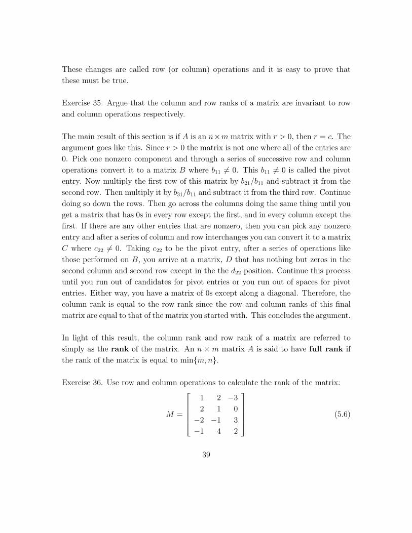
These changes are called row (or column) operations and it is easy to prove that
these must be true.
Exercise 35. Argue that the column and row ranks of a matrix are invariant to row
and column operations respectively.
The main result of this section is if A is an n×m matrix with r > 0, then r = c. The
argument goes like this. Since r > 0 the matrix is not one where all of the entries are
0. Pick one nonzero component and through a series of successive row and column
operations convert it to a matrix B where b11 6= 0. This b11 6= 0 is called the pivot
entry. Now multiply the first row of this matrix by b21/b11 and subtract it from the
second row. Then multiply it by b31/b11 and subtract it from the third row. Continue
doing so down the rows. Then go across the columns doing the same thing until you
get a matrix that has 0s in every row except the first, and in every column except the
first. If there are any other entries that are nonzero, then you can pick any nonzero
entry and after a series of column and row interchanges you can convert it to a matrix
C where c22 6= 0. Taking c22 to be the pivot entry, after a series of operations like
those performed on B, you arrive at a matrix, D that has nothing but zeros in the
second column and second row except in the the d22 position. Continue this process
until you run out of candidates for pivot entries or you run out of spaces for pivot
entries. Either way, you have a matrix of 0s except along a diagonal. Therefore, the
column rank is equal to the row rank since the row and column ranks of this final
matrix are equal to that of the matrix you started with. This concludes the argument.
In light of this result, the column rank and row rank of a matrix are referred to
simply as the rank of the matrix. An n ×m matrix A is said to have full rank if
the rank of the matrix is equal to min{m,n}.
Exercise 36. Use row and column operations to calculate the rank of the matrix:
M =
1 2 −3
2 1 0
−2 −1 3
−1 4 2
(5.6)
39

5.3 The Determinant
Square matrices are special because they are the only kinds of matrices for which
we can calculate what is called the determinant. Consider the square matrix A of
order n. Consider the (n− 1)× (n− 1) submatrix of A created by deleting row i and
column j. Call that matrix A(i, j). The (i, j)−cofactor of A is defined as
Cij(A) = (−1)i+j detA(i, j),
where detA(i, j) is the determinant of the matrix A(i, j). Now the determinant of
a 1×1 matrix is the value of the single entry. For an n×n matrix A, the determinant
is defined as
detA = a11C11(A) + ...+ a1nC1n(A). (5.7)
You may object that this definition is circular since we use the notion determinant
to define the cofactor. However, since we defined the determinant of a 1× 1 matrix,
the above equality helps us to recursively define determinants for any n× n matrix.
Exercise 37. Find a simple formula for the determinant of any 2 × 2 matrix. Use
this formula and equation (5.7) to calculate the determinant of the matrix M given
in (5.6) with the second row deleted.
Exercise 38. Show that the determinant of any lower- or upper- triangular matrix is
simply the product of the diagonal entries.
After having done Exercise 38, and knowing that you can convert a matrix into a
lower or upper triangular matrix using row and column operations, the following
properties will be useful to you in calculating the determinant of any matrix.
Let A be any square matrix of order n.
1. If the matrix B is obtained from A by interchanging any two rows (or columns)
of A then detB = − detA.
2. If B is obtained from A by multiplying each entry of some given row (or column)
of A by a nonzero constant k, then detB = k detA.
40

3. If B is obtained from A by replacing any row (or column) of A by itself plus k
times some other row (or column), where k is any number, then the determinant
remains unchanged.
4. detA = detA′
Exercise 39. Prove the four properties of determinants listed above. Then use prop-
erty 1 to show that if a matrix has a row (or column) of zeros then its determinant is 0.
Exercise 40. Show that a square matrix has full rank if and only if detA 6= 0.
5.4 Cramer’s Rule
Let [A1, ..., An] denote a square matrix A of order n with columns A1, ..., An. If
detA 6= 0 then by Exercise 40, the matrix has full rank. By row operations of the
kind described in Section 5.2 the augmented n × n + 1 matrix [A1, ..., An, v], where
v is a vector of size n can be reduced to a matrix with zeros above and below the
diagonal and 1s on the diagonal, as in1 0 · · · 0 c1
0. . . . . .
......
.... . . . . . 0
...
0 · · · 0 1 cn
.Therefore, the system of equations Ax = v where x is a vector of n variables has a
unique solution. Call it x∗. Thus
det[A1, ..., Ai−1, v, Ai+1, ..., An] = det[A1, ..., Ai−1, Ax∗, Ai+1, ..., An]
=n∑j=1
x∗j det[A1, ..., Ai−1, Aj, Ai+1, ..., An]
= x∗i detA.
which follows from the properties of determinants listed in the previous section.
Divide both sides by detA to find the solution
x∗i = det[A1, ..., Ai−1, v, Ai+1, ..., An]/ detA
for all i = 1, ..., n. This is Cramer’s rule.
41

5.5 The Inverse of a Matrix
If A is an n × n matrix with detA 6= 0 we can find a unique matrix B such that
AB = BA = In. To see why B is unique suppose that there was another matrix
C such that CA = In. Then CAB = B, but also CAB = C(AB) = CIn = C. So
B = C. The same holds if AC = In. Now we prove that B exists, and we also
calculate the entries of B.
Let ejn be the size n vector such that there is a 1 in the jth position and 0
everywhere else. Then for any n × n matrix X = [xij] solving AX = I we have
ejn = AXj where Xj is the jth column of X. Since detA 6= 0, the matrix A has full
rank (by Exercise 40), and thus the solution exists and is unique (by row reduction).
We have left to show that XA = In. By the properties of matrix multiplication and
determinants, we can find a matrix Y such that A′Y = In, which is equivalent to
Y ′A = In, and we have In = Y ′(AX)A = (Y ′A)XA = XA. We are done.
The unique matrix X = B, which is the inverse of A is denoted A−1 can be
calculated by Cramer’s rule. Note that
xij = det[A1, ..., Ai−1, ejn, Ai+1, ..., An]/ detA
= det[A1, ..., Ai−1, ejn, Ai+1, ..., An]′/ detA
= Cji(A)/ detA
Therefore, A−1 = [Cij(A)/ detA]′. Now, the following properties are useful. When-
ever inverses exist,
1. (A′)−1 = (A−1)′
2. (AB)−1 = B−1A−1
3. detA−1 = 1/ detA
4. The inverse of a lower (or upper) triangular matrix is a lower (or upper) trian-
gular matrix.
Exercise 41. Prove the four properties above and find the inverse of the matrix in
Exercise 36 (if it exists).
42

5.6 Eigenvectors and eigenvalues
Let A be a square matrix of order n. A vector of size n is an eigenvector of A if
there is a number λ such that Av = λv. If v 6= 0n then λ is unique because λ1v = λ2v
implies λ1 = λ2. In that case, λ is said to be an eigenvalue of A belonging to v.
Now here is an important result concerning determinants, eigenvectors and eigenval-
ues. Let A be a square matrix of order n. Then λ is an eigenvalue of A belonging to
some nonzero vector if and only if det(A− λI) = 0.
To see why assume that λ is an eigenvalue of A. Then by definition, there is a
vector v 6= 0 such that Av = λv. In other words, Av−λv = 0n. This implies (A−λIn)
is a matrix with linearly dependent columns (since v 6= 0), so that the rank of the
matrix is less than n. Therefore, by exercise 40 it must be that det(A− λI) = 0.
Now interpret (A − λIn)v = 0 as a set of n equations. If (A − λIn) does not
have full rank then there is at least one equation that is a linear combination of the
others. Eliminate one of the redundant equations. Now you are left with a system of
equations with more variables than unknowns, which means that at least one vari-
able can be set freely. That is equivalent to setting one entry of v freely. Make that
one entry nonzero. Therefore, there is a vector v 6= 0 such that Av = λv.
Determinants, eigenvectors and eigenvalues? Suppose A is a 2× 2 matrix
and its columns are A1 and A2. The determinant of A is the area of the parallelogram
spanned by the vectors A1 and A2. If A is a 3× 3 matrix then the determinant of A
is the volume of the parallelepiped spanned by the vectors A1, A2 and A3. If A is a
4× 4 matrix, then the determinant of A is ...
Now eigenvalues and eigenvectors. Suppose A is an n×n matrix and the solution
to det(A − λI) = 0 yields n eigenvalues λ1, λ2, ..., λn. When plugged back into
Av = λv, one can find corresponding eigenvectors associated with these eigenvalues.
Since Akv = λkv is equivalent to Av = λv for any nonzero k, these eigenvectors are
not unique. We may take ones that are normalized, i.e. ones whose lengths are set to
1. For each eigenvalue, we therefore have one eigenvector. Then create the diagonal
matrix
43

D =
λ1 0 · · · 0
0. . . . . .
......
. . . . . . 0
0 · · · 0 λn
(5.8)
and the matrix P whose first column is v1, second is v2, third is v3 etc. all the way
up to vn. Now it turns out that A = PDP−1. You may look at a proof in any
advanced linear algebra textbook or try to come up with one yourself. (Hint: If you
try to come up with your own proof, think in terms of matrices shifting axes; e.g.,
in R2 the vectors (0, 1) and (1, 0) define unit movement in the x and y directions.
Suppose we wanted to rotate our coordinate system and re-write the vector in the
new system. How would we do that?)
Exercise 42. Let
A =
[2 3
1 0
](5.9)
Find A19.
5.7 Application: Central Planning
The formal mathematical approach to central planning began with the Russian math-
ematician Leonid Kantorovich formulating of the linear programming problem. Kan-
torovich wanted to maximize a linear output function subject to linear production
constraints. (We will illustrate this today, so hang on a while if you don’t know what
that means.) He proposed the problem in his 1939 book Mathematical Method of
Production Planning and Organization and in his 1959 book, The Best Uses of Eco-
nomic Resources he argued that knowing the price of inputs and outputs is important
even when the prices are hidden, as they are in planned economies.
The most celebrated solution to the linear programming problem is the Simplex
Method, developed by American mathematician George Dantzig in 1947. This is
the method we will illustrate to solve a linear programming problem today. The
44

method gave rise to several explorations in the relationship between the planned
model and the general equilibrium model (in which prices are determined by the
market in a capitalist exchange economy).
Central planning has, with good reason, become an artifact of research and knowl-
edge from a previous era. You will likely never see the context in which I present
the Simplex method in a classroom ever again. But had we been born in a differ-
ent place at a different time, attending a public policy school to study economics
might very well have meant focusing our time and attention on the kind of problem
that I am about to show you. Since the method requires the drawing of many tables,
I illustrate the Simplex method on the blackboard with a background to the problem.
The Planning Problem. There are two goods we are interested in producing:
agricultural goods (or, for simplicity, wheat), x, and national defense goods (missiles)
y. Suppose we think that the value of a a kilo-bushel of wheat is 90, and the value
of a missile is slightly lower at 75. We want to maximize
P = 90x+ 75y.
We face production constraints. Both missiles and wheat must be produced from
inputs: land, labor and capital. Producing a missile takes 3 units of labor, 9 units of
capital and 2 units of land. Producing a kilo-bushel of wheat takes 2 units of labor,
4 units of capital and 10 units of land. Suppose we have with us only a total of 66
units of labor, 180 units of capital and 200 units of land. The constraints can thus
be represented
3x+ 2y ≤ 66
9x+ 4y ≤ 180
2x+ 10y ≤ 200
x ≥ 0, y ≥ 0
First we draw the constraints on the blackboard (see board) and solve the problem
geometrically. Now, it wouldn’t be in the spirit of a central planning model if I told
you how the simplex method works before demonstrating it, so let me show you how
to solve the problem by setting up a matrix algorithm.
45

The steps to follow in the algorithm are as follows. First, write the inequality
constraints as equalities with slack variables.
3x+ 2y + s1 = 66
9x+ 4y + s2 = 180
2x+ 10y + s3 = 200
x ≥ 0, y ≥ 0, si ≥ 0∀i
(It will be useful for you to remember the concept of a slack variable when we do
non-linear programming next week.) Then write the first equation as:
−90x+ 70y + P = 0.
Form the augmented matrix of coefficients:
x y s1 s2 s3 P
3 2 1 0 0 0 66
9 4 0 1 0 0 180
2 10 0 0 1 0 200
-90 -75 0 0 0 1 0
Now follow this process:
1. Find the least of the negative numbers in the bottom row (choosing any in case
of a tie). The column containing this number is the pivot column.
2. Divide each entry in the last column (except the one in the last row) by the
corresponding number in the pivot column as long as the number in the pivot
column is positive. The row with the lowest quotient is the pivot row. In case
of a tie, pick either one. If the pivot column does not have any positive entries
above the last row, then stop; the problem has no solution.
3. The pivot element is the element in the pivot column and pivot row. Perform
row operations on the matrix so that there is a 1 where the pivot element is
and 0 everywhere else in the pivot column. Look at the bottom row. If all
entries are nonnegative then you have found a solution; so stop. Otherwise, go
back to step 1.
46

At a solution, each variable under which there are 0s everywhere except a 1 in some
spot take the corresponding value on the right most column. The number on the
bottom right is the value of the objective function at the solution.
What is going on in the simplex method? Mostly magic; but each time you pivot
around an entry in the matrix you are moving from one point on the constraint
boundary to another. It is your job, for homework, to figure out how exactly the
row operations do this. Think in terms of equations.
Exercise 43. What is going on in the simplex method? What is the main problem
with using linear programming to plan an economy?
47

Chapter 6
Integration
6.1 Upper and Lower Sums
Let S = [a, b] be a closed interval, and let f be a function that is bounded on S, i.e.
there is a number, C, such that |f(x)| ≤ C for all x ∈ S. A partition of [a, b] is a
set P of points x0, x1, ..., xn such that
a = x0 < x1 < ... < xn = b.
A refinement of a partition P is another partition P ′ such that P ⊂ P ′. Define
L(f, P ) =∑n
k=1mk(xk − xk−1), where mk = inf{f(x)|x ∈ [xk−1, xk]},U(f, P ) =
∑nk=1Mk(xk − xk−1), where Mk = sup{f(x)|x ∈ [xk−1, xk]}.
Now if P and P ′ are partitions of S and P ′ is a refinement of P , then
L(f, P ) ≤ L(f, P ′) ≤ U(f, P ′) ≤ U(f, P ). (6.1)
This is easy to see geometrically. In fact, the coarsest partition bounds the set of all
L(f, P ) and U(f, P ) with respect to partitions, since
m(b− a) ≤ L(f, P ) ≤ U(f, P ) ≤M(b− a),
where m = inf{f(x)|x ∈ S} and M = sup{f(x)|x ∈ S}. Now, define
L(f) = supP{L(f, P )} and U(f) = infP{U(f, P )}.
48

It is easy to see that L ≤ U . The argument is as follows. For a fixed partition P ∗,
L(f, P ∗) is a lower bound for the set of U(f, P ), because for any two partitions P
and P ′, there is a refinement of both of them, P ′′, which by (6.1), leads to
L(f, P ) ≤ L(f, P ′′) ≤ U(f, P ′′) ≤ U(f, P ′).
Therefore, L(f, P ) ≤ U , and this is true for every P , completing the argument.
Now a bounded function, f : S → R, is Riemann integrable if L(f) = U(f).
If this is the case, the common value is denoted∫Sf(x)dx or
∫ baf(x)dx.
6.2 Integrability of Continuous Functions
We now prove an important result: If S = [a, b] and f : S → R is continuous, then
it is Riemann integrable. But first I argue the claim that f is Riemann integrable
on S = [a, b] if and only if for all ε > 0 there is a partition P such that
U(f, P )− L(f, P ) < ε. (6.2)
Start by assuming that f is Riemann integrable on [a, b], and let’s try to obtain
the implication. Let
I =
∫ b
a
f(x)dx. (6.3)
Take any ε > 0. Since L = U , it follows that there must be partitions P ′ and P ′′
such that
I − ε2< L(f, P ′) and U(f, P ′′) < I + ε
2.
Now let P be a refinement of both P ′ and P ′′. Then
I − ε2< L(f, P ′) ≤ L(f, P ) ≤ U(f, P ) < U(f, P ′′) < I + ε
2,
which is just a simple application of (6.1). From this we get I < L(f, P ) + ε2
and
U(f, P )− ε2< I, which when combined gives us U(f, P )− L(f, P ) < ε. Check.
We can go the other way now. Assume that (6.2) is true. By definition, U ≤U(f, P ) for any P and L ≥ L(f, P ) for any P . U(f, P ) ≥ L(f, P ) and U ≥ L, so it
must be that 0 ≤ U − L < ε. But ε is arbitrary, so U = L. Therefore, f is Riemann
integrable.
49

Exercise 44. To continue the proof, we need to introduce a new concept. A function
f : [a, b] → R is uniformly continuous if for all ε > 0 there is δ > 0 such that
if x, y ∈ [a, b] and |x − y| < δ, then |f(x) − f(y)| < ε. This differs from regular
continuity in that here δ does not depend on x, whereas in the regular case it may.
Show that if f : [a, b]→ R is continuous, then it is uniformly continuous.
Now we are going to use (6.2) to prove that continuous functions are integrable.
Since f is uniformly continuous (see Exercise 44), we know that for any ε > 0 there
is δ > 0 such that |x − y| < δ implies |f(x) − f(y)| < ε/(b − a), where x and y are
elements of S. (It doesn’t matter that we divided ε by b− a; if you don’t like that,
you could have chosen (b − a)ε instead; it was arbitrary after all.) Now for any ε
take the associated δ and partition the interval [a, b] into n subintervals, each of size
l < δ. By definition, the mk and Mk differ by at most ε/(b− a). Therefore,
U(f, P )− L(f, P ) =n∑k=1
(Mk −mk)(xk − xk−1)
<n∑k=1
ε
b− al =
ε
b− a
n∑k=1
l = ε,
and we’re done. Now one thing that I’m not going to prove but that you should
know is that if a bounded function is continuous except at a finite number of points,
then it is integrable. There are even stronger results, but for now just relax.
6.3 Properties of the Integral
Let f and g be Riemann integrable functions on [a, c] and let k ∈ R. Then
1.∫ cakf(x)dx = k
∫ caf(x)dx
2.∫ ca[f(x) + g(x)]dx =
∫ caf(x)dx+
∫ cag(x)dx
3. The same as (2) but with minus signs.
4. |∫ caf(x)dx| ≤
∫ ca|f(x)|dx
5.∫ caf(x)dx ≤
∫ cag(x)dx if f(x) ≤ g(x) for all x ∈ [a, c]
50
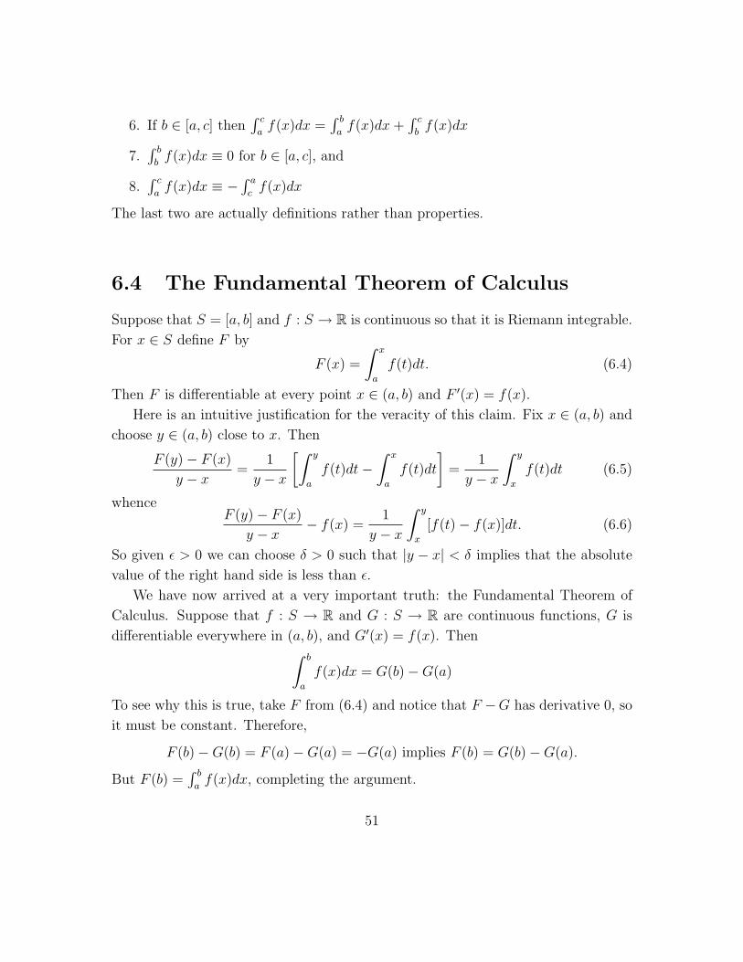
6. If b ∈ [a, c] then∫ caf(x)dx =
∫ baf(x)dx+
∫ cbf(x)dx
7.∫ bbf(x)dx ≡ 0 for b ∈ [a, c], and
8.∫ caf(x)dx ≡ −
∫ acf(x)dx
The last two are actually definitions rather than properties.
6.4 The Fundamental Theorem of Calculus
Suppose that S = [a, b] and f : S → R is continuous so that it is Riemann integrable.
For x ∈ S define F by
F (x) =
∫ x
a
f(t)dt. (6.4)
Then F is differentiable at every point x ∈ (a, b) and F ′(x) = f(x).
Here is an intuitive justification for the veracity of this claim. Fix x ∈ (a, b) and
choose y ∈ (a, b) close to x. Then
F (y)− F (x)
y − x=
1
y − x
[∫ y
a
f(t)dt−∫ x
a
f(t)dt
]=
1
y − x
∫ y
x
f(t)dt (6.5)
whenceF (y)− F (x)
y − x− f(x) =
1
y − x
∫ y
x
[f(t)− f(x)]dt. (6.6)
So given ε > 0 we can choose δ > 0 such that |y − x| < δ implies that the absolute
value of the right hand side is less than ε.
We have now arrived at a very important truth: the Fundamental Theorem of
Calculus. Suppose that f : S → R and G : S → R are continuous functions, G is
differentiable everywhere in (a, b), and G′(x) = f(x). Then∫ b
a
f(x)dx = G(b)−G(a)
To see why this is true, take F from (6.4) and notice that F −G has derivative 0, so
it must be constant. Therefore,
F (b)−G(b) = F (a)−G(a) = −G(a) implies F (b) = G(b)−G(a).
But F (b) =∫ baf(x)dx, completing the argument.
51
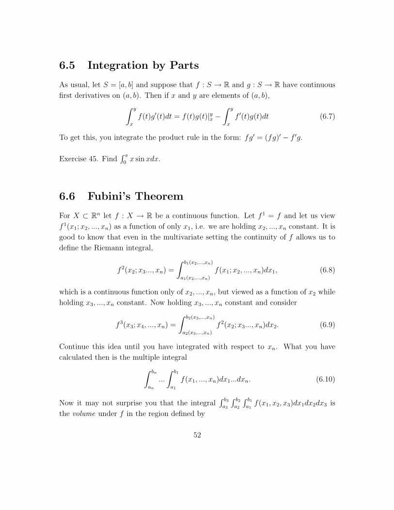
6.5 Integration by Parts
As usual, let S = [a, b] and suppose that f : S → R and g : S → R have continuous
first derivatives on (a, b). Then if x and y are elements of (a, b),∫ y
x
f(t)g′(t)dt = f(t)g(t)|yx −∫ y
x
f ′(t)g(t)dt (6.7)
To get this, you integrate the product rule in the form: fg′ = (fg)′ − f ′g.
Exercise 45. Find∫ π
0x sinxdx.
6.6 Fubini’s Theorem
For X ⊂ Rn let f : X → R be a continuous function. Let f 1 = f and let us view
f 1(x1;x2, ..., xn) as a function of only x1, i.e. we are holding x2, ..., xn constant. It is
good to know that even in the multivariate setting the continuity of f allows us to
define the Riemann integral,
f 2(x2;x3..., xn) =
∫ b1(x2,...,xn)
a1(x2,...,xn)
f(x1;x2, ..., xn)dx1, (6.8)
which is a continuous function only of x2, ..., xn, but viewed as a function of x2 while
holding x3, ..., xn constant. Now holding x3, ..., xn constant and consider
f 3(x3;x4, ..., xn) =
∫ b2(x3,...,xn)
a2(x3,...,xn)
f 2(x2;x3..., xn)dx2. (6.9)
Continue this idea until you have integrated with respect to xn. What you have
calculated then is the multiple integral∫ bn
an
...
∫ b1
a1
f(x1, ..., xn)dx1...dxn. (6.10)
Now it may not surprise you that the integral∫ b3a3
∫ b2a2
∫ b1a1f(x1, x2, x3)dx1dx2dx3 is
the volume under f in the region defined by
52

X = {(x1, x2, x3)|ai ≤ xi ≤ bi, i = 1, 2, 3} ⊂ R3.
Since it does not matter how we compute this quantity, Fubini’s theorem tells
us that if f is continuous on the region X, then which variables you integrate
with respect to first does not matter, you get the same answer at the end. This
generalizes to n-dimensional volume, i.e. Fubini’s theorem is also true if instead
X = {(x1, ..., xn)|ai ≤ xi ≤ bi, i = 1, ..., n} ⊂ Rn and we wanted to calculate the
multiple integral in (6.10).
6.7 The Change of Variables
Suppose that g is differentiable on the open interval (a, b) and that its derivative is
continuous. Let T be an open interval such that g(x) ∈ T for all x ∈ (a, b). If a
function f is continuous on T then the composition f(g) is continuous on (a, b), and∫ b
a
f(g)(x)g′(x)dx =
∫ g(b)
g(a)
f(g)dg (6.11)
which you get by integrating the chain rule.
Exercise 46. Find∫ 1
0x(1− x2)0.5dx.
The change of variables theorem generalizes in the following way. Let x = f(v)
where v is a vector of size n. Suppose that g : A′ → A is an injective function with
continuous partial derivatives, where A′ ⊂ Rn and A ⊂ Rn. In other words, g is
defined by
g[(v1, ..., vn)′] = (g1(v1), ..., gn(vn))′ = (x1, ..., xn)
where gi is a function gi : A′ → R, such that gi(vi) = xi for all i = 1, ..., n. Suppose
that the Jacobian matrix, J = [∂gi/∂vj]j=1,...,ni=1,...,n , is invertible (i.e. has an inverse) for
all v ∈ A′. Then if we wanted to calculate the volume under the function f(x) in
the region A, we can do so by calculating the right hand side of∫...∫Af(x)dx1...dxn =
∫...∫A′f(g1(v), ..., gn(v))| det J |dv1...dvn,
53

which may be easier than calculating the left hand side. (Sometimes it may just not
be possible to calculate the left hand side.) The only difficulty is that it is up to us
to find the best change of variables, i.e. the function g, that makes the calculation
possible or easiest.
Exercise 47. Let A′ be the region:
A′ = {x ∈ R2|y ≥ −x− 1, y ≤ −x+ 1, y ≥ x− 1, y ≤ x+ 1}
Now calculate ∫ ∫A′
(x− y
x+ y + 2
)2
dxdy. (6.12)
6.8 Improper Integrals
You will be pleased to know that if f is Riemann integrable on the interval [a, b] is
integral on (a, b], [a, b) and (a, b), are all defined to be the same as its integral on
[a, b]. You will also be pleased to know that a = −∞ and/or b = ∞ are allowed so
long as you remember that∫∞af(x)dx is really limb→∞
∫ baf(x)dx and
∫ b−∞ f(x)dx is really lima→∞
∫ baf(x)dx.
6.9 Taylor’s Theorem
Let S be an open interval and let f : S → R be a function whose first, second,...,
and mth derivatives exist and are all continuous. Denote the jth derivative of f by
f (j). For a ∈ S and b ∈ S, and n ≤ m we have
f(b) = f(a) +f ′(a)
1!(b− a) + ...+
f (n−1)(a)
(n− 1)!(b− a)n−1 +Rn (6.13)
where
Rn =
∫ b
a
(b− t)n−1
(n− 1)!f (n)(t)dt. (6.14)
Here is the proof. The fundamental theorem of calculus tells us that f(b) = f(a) +∫ baf ′(t)dt. Notice that this is equation (6.13) for n = 1. Now assume that (6.13) is
54

true. Perform the integration in (6.14) by parts where the function whose derivative
is not taken is f (n)(t), and the derived function is (b−t)n−1
(n−1)!. If you do this you get
Rn =(b− a)n
n!f (n)(a) +
∫ b
a
(b− t)n
n!f (n+1)(t)dt. (6.15)
Plug this back into (6.13) and, by induction, you have completed the proof.
Exercise 48. Assume in the above theorem that S contains 0 and remember that
because f (n)(x) is continuous and [a, b] is compact, the function is bounded. Argue
that under these conditions, the Taylor polynomial
Pn−1(x) = f(0) + f ′(0)x+f (2)(0)
2!x2 + ...+
f (n−1)(0)
(n− 1)!xn−1 (6.16)
is a good approximation of f when n is large.
Exercise 49. Recall from the Weierstrass Theorem that because it is continuous, f
attains a maximum and a minimum on the interval [a, b]. Use the intermediate value
theorem to show that there is a number c ∈ [a, b] such that
Rn = f (n)(c)(b− a)n
n!. (6.17)
What does this say for (6.13)?
Taylor’s theorem in Rn. Let f : S → R, where S ⊂ Rn is an open set. If f is C1
then for any x ∈ S and y ∈ S, we can write
f(y) = f(x) +∇f(x)(y − x) +R1(x, y), (6.18)
where R1 is a function with the property
limy→x
(R1(x, y)
||x− y||
)= 0. (6.19)
If f is C2 then for any a ∈ S and b ∈ S, we can write
f(y) = f(x) +∇f(x)(y − x) +1
2(y − x)′Hf(x)(y − x) +R2(x, y), (6.20)
55

where Hf(x) is the Hessian matrix and R2 is a function with the property
limy→x
(R2(x, y)
||x− y||2
)= 0. (6.21)
Here limy→x is abusive limit for the convergence of vectors that was defined yesterday.
I will prove only the first part of the statement, leaving the second part as an exercise.
Here goes. Since R1(x, y) was not defined (it is a residual term) all we have to show
is that (64) is true. Now fix x and define h(y) = f(y) − f(x) +∇f(x)(y − x), and
notice that h(x) = 0. Then showing (64) is equivalent to showing that for any ε > 0
there is a δ such that y ∈ S and
||y − x|| < δ imply |h(y)| < ε||x− y||,
and this is what we’ll show.
By the continuity of ∇h (why is ∇h continuous?) there is a δ > 0 such that
y ∈ S and
||y − x|| ≤ δ imply ||∇h(y)|| < ε.
Now for any y ∈ S such that ||y − x|| < δ, define g : [0, 1]→ R by
g(t) = h[(1− t)x+ ty].
(For math geeks, why is g well defined?) Then g(0) = h(x) = 0. Now g is differen-
tiable because h is, and
g′(t) = ∇h[(1− t)x+ ty](y − x). (6.22)
Now notice that ||(1− t)x+ ty−x|| = t||y−x|| < δ for all t ∈ [0, 1]. So by continuity,
||∇h[(1− t)x+ ty]|| ≤ ε for all t ∈ [0, 1], which means that |g′(t)| < ε||y − x|| for all
t ∈ [0, 1].
By the mean value theorem in R, there is a c such that
g(1) = g(0) + g′(c).
Therefore, |h(y)| = |g(1)| = |g′(c)| < ε||y − x||, and we are done.
Exercise 50. Write down three terms of the Taylor series and evaluate the it at
(x, y) = (1, 1) for f(x, y) = ln(xy).
56

Chapter 7
Optimization
7.1 Optimization in RLet S ⊂ R and f : S → R be differentiable function on the interior of S. The interior
of a set A ⊂ Rn is the set
A∗ = {x ∈ A|∃ an open box B such that x ∈ B and B ⊂ A}.
If f achieves a maximum or minimum in the interior of S then f ′(x) = 0 at the
point x at which it achieves a maximum or minimum. If x ∈ S∗ is a maximum then
f ′′(x) ≤ 0. If it is a minimum then f ′′(x) ≥ 0. Note that f ′(x) = 0 and f ′′(x) ≤ 0 are
only necessary conditions for x ∈ S∗ being a maximum. The next exercise demon-
strates how they are insufficient.
Exercise 51. Let f : [−2, 5] → R be defined by f(x) = x3 − 4.5x + 6x + 1. By
the Weierstrass theorem we know that f achieves a maximum and minimum on its
domain. We can find the values of x where f ′(x) = 0. Which of these are maximum
values of f and minimum values of f? Calculate f(x) at the points where f ′(x) = 0.
Then calculate f(−1) and f(4).
What are the issues with sufficiency? The problem is that of global versus local
minima and maxima. One popular way of avoiding this problem is to assume that S
is a convex set and f is either a concave or convex function. In that case, if f ′(x) = 0
57
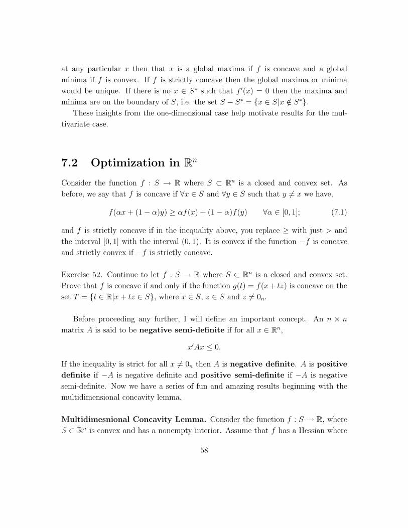
at any particular x then that x is a global maxima if f is concave and a global
minima if f is convex. If f is strictly concave then the global maxima or minima
would be unique. If there is no x ∈ S∗ such that f ′(x) = 0 then the maxima and
minima are on the boundary of S, i.e. the set S − S∗ = {x ∈ S|x /∈ S∗}.These insights from the one-dimensional case help motivate results for the mul-
tivariate case.
7.2 Optimization in Rn
Consider the function f : S → R where S ⊂ Rn is a closed and convex set. As
before, we say that f is concave if ∀x ∈ S and ∀y ∈ S such that y 6= x we have,
f(αx+ (1− α)y) ≥ αf(x) + (1− α)f(y) ∀α ∈ [0, 1]; (7.1)
and f is strictly concave if in the inequality above, you replace ≥ with just > and
the interval [0, 1] with the interval (0, 1). It is convex if the function −f is concave
and strictly convex if −f is strictly concave.
Exercise 52. Continue to let f : S → R where S ⊂ Rn is a closed and convex set.
Prove that f is concave if and only if the function g(t) = f(x+ tz) is concave on the
set T = {t ∈ R|x+ tz ∈ S}, where x ∈ S, z ∈ S and z 6= 0n.
Before proceeding any further, I will define an important concept. An n × n
matrix A is said to be negative semi-definite if for all x ∈ Rn,
x′Ax ≤ 0.
If the inequality is strict for all x 6= 0n then A is negative definite. A is positive
definite if −A is negative definite and positive semi-definite if −A is negative
semi-definite. Now we have a series of fun and amazing results beginning with the
multidimensional concavity lemma.
Multidimesnional Concavity Lemma. Consider the function f : S → R, where
S ⊂ Rn is convex and has a nonempty interior. Assume that f has a Hessian where
58
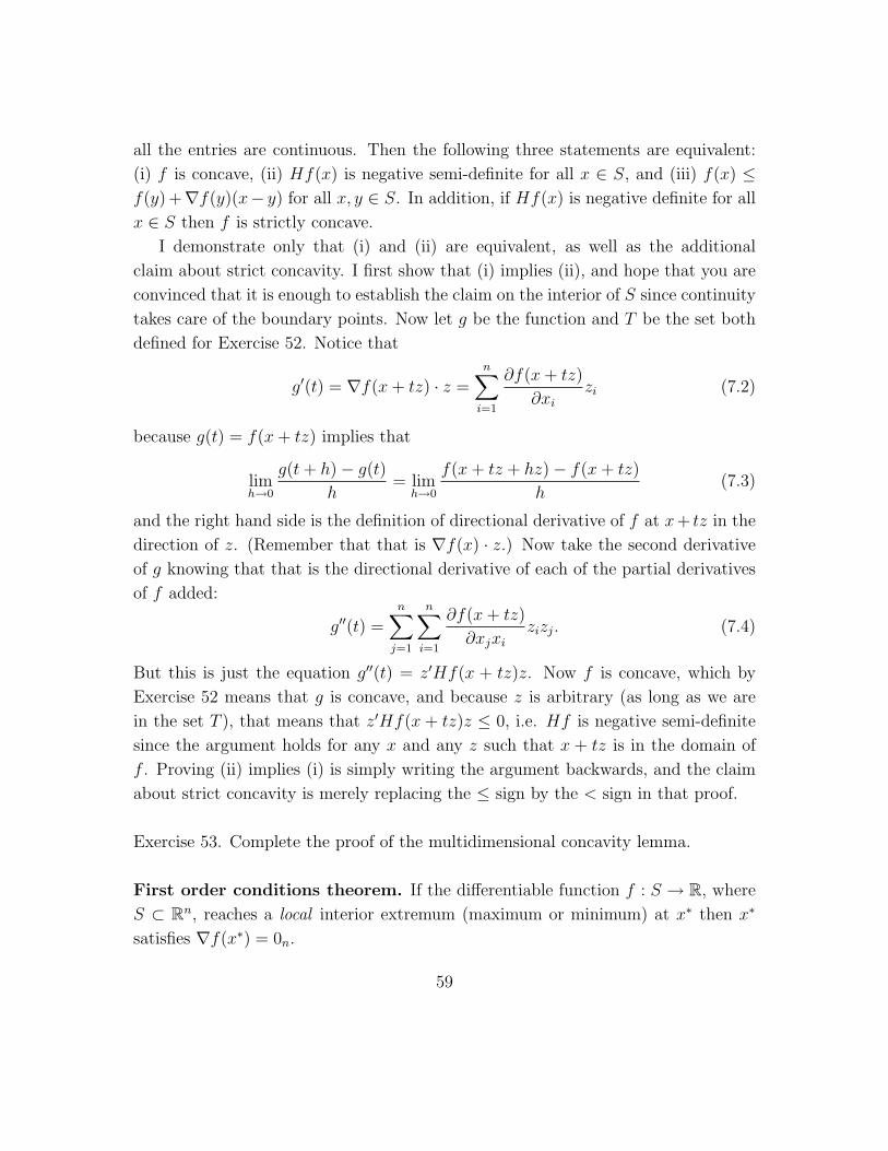
all the entries are continuous. Then the following three statements are equivalent:
(i) f is concave, (ii) Hf(x) is negative semi-definite for all x ∈ S, and (iii) f(x) ≤f(y) +∇f(y)(x− y) for all x, y ∈ S. In addition, if Hf(x) is negative definite for all
x ∈ S then f is strictly concave.
I demonstrate only that (i) and (ii) are equivalent, as well as the additional
claim about strict concavity. I first show that (i) implies (ii), and hope that you are
convinced that it is enough to establish the claim on the interior of S since continuity
takes care of the boundary points. Now let g be the function and T be the set both
defined for Exercise 52. Notice that
g′(t) = ∇f(x+ tz) · z =n∑i=1
∂f(x+ tz)
∂xizi (7.2)
because g(t) = f(x+ tz) implies that
limh→0
g(t+ h)− g(t)
h= lim
h→0
f(x+ tz + hz)− f(x+ tz)
h(7.3)
and the right hand side is the definition of directional derivative of f at x+ tz in the
direction of z. (Remember that that is ∇f(x) · z.) Now take the second derivative
of g knowing that that is the directional derivative of each of the partial derivatives
of f added:
g′′(t) =n∑j=1
n∑i=1
∂f(x+ tz)
∂xjxizizj. (7.4)
But this is just the equation g′′(t) = z′Hf(x + tz)z. Now f is concave, which by
Exercise 52 means that g is concave, and because z is arbitrary (as long as we are
in the set T ), that means that z′Hf(x + tz)z ≤ 0, i.e. Hf is negative semi-definite
since the argument holds for any x and any z such that x + tz is in the domain of
f . Proving (ii) implies (i) is simply writing the argument backwards, and the claim
about strict concavity is merely replacing the ≤ sign by the < sign in that proof.
Exercise 53. Complete the proof of the multidimensional concavity lemma.
First order conditions theorem. If the differentiable function f : S → R, where
S ⊂ Rn, reaches a local interior extremum (maximum or minimum) at x∗ then x∗
satisfies ∇f(x∗) = 0n.
59

The proof goes as follows. Again write f(x∗ + tz) in terms of the familiar g of
Exercise 52 (yes, this time x∗ instead of x). Note that g(0) = f(x∗). Because g
coincides with some value of f for every t, then g(t) must reach a local extremum at
t = 0 if f reaches an extremum at x. This means that g′(0) = 0. Now recall from the
proof of the multidimensional concavity lemma why it should be that (7.2) should
hold with x replaced by x∗. Combined with g′(0) = 0, this implies that ∇f(x∗)z = 0.
Since this holds for any z, it must hold for all ej, j = 1, .., n. Therefore, each of the
partials are 0, and we have ∇f(x∗) = 0n.
Second order conditions theorem. If the C2 function f : S → R, where S ⊂ Rn,
reaches a local interior maximum (resp. minimum) at x∗, then Hf(x∗) is negative
(positive) semidefinite.
Here is the proof. Recall that (7.4) must be true. Then if f is maximized at
x = x∗ it must be that g is maximized at t = 0, and thus g′′(0) ≤ 0. That means
that the right hand side of (7.4) is nonpositive, or that the Hessian of f at x∗ is
negative semidefinite. (This is again because z is arbitrary.) A similar argument
holds for the “minimized” case.
Global maximum theorem. If the C2 function f : S → R, where S ⊂ Rn, has a
negative semidefinite Hessian at every x in the interior of S, then ∇f(x∗) = 0 implies
that f achieves a global maximum at x∗.
Proof. Because the Hessian is everywhere negative semidefinite, f is concave
by the multidimensional concavity lemma. The same lemma tells us that f(x) ≤f(x∗) +∇f(x∗)(x− x∗) for all x ∈ S. Now if ∇f(x∗) = 0n then f(x) ≤ f(x∗) for all
x ∈ S. So f reaches a global maximum.
A similar theorem holds for global minima. However, in most applications if what
you are using the first and second order conditions to find interior minima of f , you
can do this by finding interior maxima of −f .
Exercise 54. Re-read the proof of the global maximum theorem. Then prove that if
the Hessian of f is negative definite at every x in its domain, and x∗ maximizes f ,
then x∗ is the unique global maximizer of f .
60

Definiteness of the Hessian. Let D1(x) be the determinant of the top left 1× 1
submatrix of the n×n matrix Hf(x), D2(x) be the determinant of the top left 2× 2
submatrix of Hf(x),..., and Dk(x) be the determinant of the top left k×k submatrix
of Hf(x). If (−1)iDi(x) > 0 for all i = 1, ..., n then Hf(x) is negative definite, and
if this is true for all x in the domain of f then f is strictly concave. If Di(x) > 0
for all i = 1, ..., n then Hf(x) is positive definite, and if this is true for all x in the
domain of f then f is strictly convex.
Exercise 55. Provide an argument for the definiteness of the claim above.
7.3 Lagrange’s Theorem
Let S ⊂ Rn. Let f : S → R and gi : S → R, i = 1, ..., k, be C1 functions. Let x∗
be a point in the interior of S and suppose that x∗ is an optimum (local maximum
or local minimum) of f subject to the constraints, gi(x) = 0, i = 1, ..., k. If the
gradient vectors ∇gi(x∗), i = 1, ..., k, are linearly independent then there exists a
vector Λ = (λ1, ..., λk)′ ∈ Rk such that
∇f(x∗) +k∑i=1
λi∇gi(x∗) = 0 (7.5)
Intuition. Recall that S∗ denotes the interior of S and write the problem as
maxx∈S∗ f(x) subject to gi(x) = 0, i = 1, ..., k.
Now define the Lagrangean for this problem,
L(x,Λ) = f(x) +∑k
i=1 λigi(x),
and apply the first order conditions theorem to L while deleting the last equation:
∇nL(x,Λ) = ∇f(x) +k∑i=1
λi∇gi(x) = 0, (7.6)
61

where ∇nL simply means the vector with only the first n entries of usual gradient
of L, since differentiating with respect to Λ gives us back the constraints. Thus the
information that we discard was something we already knew.
Now we have to convince ourselves of two things. First, we must be convinced
that the solution to the maximization problem, x is a vector of the first n entries
of a critical point of L(x,Λ). To convince yourself, understand that the directional
derivative ∇f(x) · h = 0 at the maximum for all small length vectors h that take x
to points in which the constraints gi continue to be satisfied. If the gi continue to be
satisfied after moving a small amount in the direction h then, then no change occurs in
any gi, i.e. ∇gi·h = 0 for all i = 1, ..., k. But that means that∇nL(x,Λ)·h = ∇f(x)·hfor any movement h that keeps the constraints satisfied. This is good. It says that
you cannot increase or decrease the objective function f by making small movements
in any “permissible” direction. So we must be at a critical point of L (except that
we don’t know the λi). Suppose we were at a maximum or minimum at x. Then the
constraints would be satisfied and so would (7.5).
The second thing that we must convince ourselves is that the vector Λ exists.
That’s a little harder, and you will have to wait until we see the proof of the theorem.
Caution with Lagrange. Let f : R2 → R be the function f(x, y) = −y and
g : R2 → R be the function g(x, y) = y3−x2. Notice that the maximum of f subject
to g(x, y) = 0 is at (0, 0), since if y is negative x would have to be the square root of
a negative number for the constraint to be met. If you set up the Lagrangean, L of
this problem (defined in the previous lecture note) and take the first order conditions
then you get
−2λx = 0
−1 + 3λy2 = 0
−x2 + y3 = 0
Now for the first equation to be true, either λ = 0 or x = 0. If λ = 0 then the second
equation is a contradiction. If x = 0 then the third implies that y = 0. Plug this
back into the second and obtain a contradiction again.
Exercise 56. What went wrong in the example above?
62

Now suppose that f is defined by
f(x, y) =1
3x3 +
3
2y2 + 2x (7.7)
instead, and g was the benign g(x, y) = x − y. The constraint qualification is met
since ∇g(x, y) = (1,−1) for all x and y. Now set up the Lagrangean and take the
first order conditions:
x2 + 2− λ = 0
−3y − λ = 0
x− y = 0
There are two solutions: (x, y) = (2, 2) or (1, 1), and seeing that f(2, 2) = 2/3 while
f(1, 1) = 5/6 you could guess that (2, 2) is a minimum and (1, 1) is a maximum. But
in fact, f(0, 0) = 0 and f(3, 3) = 1.5.
Exercise 57. What went wrong here?
7.4 The Karush-Kuhn-Tucker Theorem
In most economic applications constraints to a maximization problem take the form
of inequalities rather than equalities. Begin with the simple problem
maxx f(x) subject to x ≥ 0
and notice that if x∗ is the solution then it satisfies one of the following three cases:
1. x∗ = 0 and f ′(x∗) < 0,
2. x∗ = 0 and f ′(x∗) = 0,
3. x∗ > 0 and f ′(x∗) = 0.
63

These imply that
1. f ′(x∗) ≤ 0,
2. x∗[f ′(x∗)] = 0,
3. x∗ ≥ 0.
In the world of Rn, these correspond to
1. ∂f(x∗)∂xi≤ 0,
2. x∗i
[∂f(x∗)∂xi
]= 0, and
3. x∗i ≥ 0,
which must hold for all i = 1, ..., n if x∗ maximizes f(x) subject to xi ≥ 0 for all i.
Now convince yourself that the problem
maxx1,x2 f(x1, x2) subject to g(x1, x2) ≥ 0,
is equivalent to
maxx1,x2,z f(x1, x2) subject to g(x1, x2)− z = 0 and z ≥ 0.
(Where have we seen the use of a slack variable like z before?) Take the first order
conditions of the Lagrangian, L of this latter beast while ignoring the inequality
constraint, and arrive at
∂f
∂x1
+ λ∂g
∂x1
= 0
∂f
∂x2
+ λ∂g
∂x2
= 0
∂f
∂λ= g(x1, x2)− z = 0
These give the critical points of L. The only additional necessary conditions come
from the inequality constraint z ≥ 0. The insight from the previous discussion tells
us the equivalent of properties (1)− (3) for z, i.e that:
−λ ≤ 0
z(−λ) = 0
z ≥ 0
64

Summarizing, we have:
∂f
∂x1
+ λ∂g
∂x1
= 0
∂f
∂x2
+ λ∂g
∂x2
= 0
λg(x1, x2) = 0
λ ≥ 0
g(x1, x2) ≥ 0
These are called the Karush-Kuhn-Tucker conditions. More generally, we have:
The Karush-Kuhn-Tucker Theorem. Let S ⊂ Rn and f : S → R and gi :
S → R, i = 1, ..., k, be C1 functions. Let x∗ be a point in the interior of S and
suppose that x∗ is an optimum (local maximum or local minimum) of f subject to
the constraints, gi(x) ≥ 0, i = 1, ..., k. If the gradient vectors ∇gi(x∗), i = 1, ..., k,
are linearly independent then there exists a vector Λ = (λ1, ..., λk)′ ∈ Rk such that
∇f(x∗) +∑k
i=1 λi∇gi(x∗) = 0 and λigi(x∗) = 0 for all i = 1, ..., k.
In addition, the λi are all nonnegative if x∗ is a maximum and nonpositive if it is a
minimum.
Exercise 58. Re-read the cautionary examples for Lagrange and consider the problem
of finding (x, y) to maximize f(x, y) = −(x2 +y2) subject to h(x, y) = (x−1)3−y2 ≥0. Find a solution to this problem just by looking at the functions. (You don’t have
to set up any Lagrangean or Karush-Kuhn-Tucker conditions). Now show that this
problem cannot be analyzed using the Karush-Kuhn-Tucker theorem. Which one of
the assumptions is violated?
65

7.5 Proof of Lagrange’s Theorem
We prove the statement only for k = 1. Let g(x) = g1(x) so that we can drop the
subscript from now on. Let the local optimum be x∗. The rank condition on g tells
us that ∇g(x∗) 6= 0n. Without loss of generality, assume that the first component of
this vector is nonzero. Denote the first coordinate of a vector
x ∈ D ≡ S ∩ {x ∈ Rn|g(x) = 0}
by w and the last n − 1 of them by z. Write x = (w, z). Let x∗ = (w∗, z∗) denote
the local optimum. Let ∇fw(w, z) denote the derivative of f with respect to w alone
and ∇fz(w, z) denote the derivative with respect to z alone. The derivative of g is
partitioned analogously into ∇gw(w, z), which is a number, and ∇gz(w, z) which is
a vector of size n− k.
To prove the theorem we must show that there exists λ ∈ R such that
1. ∇fw(w∗, z∗) + λ∇gw(w∗, z∗) = 0
2. ∇fz(w∗, z∗) + λ∇gz(w∗, z∗) = 0
To prove this we need to appeal to the Implicit Function Theorem. This says that
there is an open box B ∈ Rn−1 containing z∗ and a C1 function h : B → R such that
h(z∗) = w∗ and g(h(z), z) = 0 for all z ∈ B. Also,
∇h(z) = −∇gz(h(z), z)
∇gw(h(z), z)(7.8)
which you will recognize as none other than formula (4.12).
Define λ now as
λ = −∇fw(w∗, z∗)
∇gw(w∗, z∗)
which rearranges to
∇fw(w∗, z∗) + λ∇gw(w∗, z∗) = 0.
That’s the first thing we had to show, which is a bit simpler than the second. Define
the function φ : B → R by φ(z) = f(h(z), z). Since f has a local optimum at
(w∗, z∗) = (h(z∗), z∗), then φ has a local optimum at z∗. Since B is open, z∗ is an
66

unconstrained local optimum of φ and the first-order conditions for an unconstrained
optimum imply ∇φ(z∗) = 0n−1, i.e. by the chain rule:
∇fw(w∗, z∗)∇h(z∗) +∇fz(w∗, z∗) = 0. (7.9)
Substitute (7.8) in this to get
∇fz(w∗, z∗) + λ∇gz(w∗, z∗) = 0.
and that’s it.
Exercise 59. We did not prove the Chain rule appearing in (7.9) in the multidimen-
sional case. In the case of two variables, let x(t), y(t) be two differentiable functions of
t and let f(x, y) be a differentiable function. For the purposes of this demonstration,
define ∂x = x(t+ h)− x(t) and ∂y = y(t+ h)− y(t). Then
f ′(x(t), y(t)) = limh→0
f(x(t+ h), y(t+ h))− f(x(t), y(t))
h
= limh→0
f(x+ ∂x, y + ∂y)− f(x, y + ∂y) + f(x, y + ∂y)− f(x, y)
h
= limh→0
f(x+ ∂x, y + ∂y)− f(x, y + ∂y)
h+ lim
h→0
f(x, y + ∂y)− f(x, y)
h.
On the right is the definition of the partial of f with respect to y, which by the single
variable chain rule is∂f
∂y
dy
dt.
Apply the mean value theorem to the limit on the left by picking an x′ ∈ [x, x+ ∂x]
such that the limit is equal to
limh→0
∂x
h
∂f(x′)
∂x=∂f
∂x
dx
dt.
That gives us
f ′(x(t), y(t)) =∂f
∂x
dx
dt+∂f
∂y
dy
dt.
Use an extended argument based on this demonstration to argue that (7.9) is true.
67

7.6 Second Order Conditions
Let us make a few modifications to Lagrange’s Theorem. Instead of assuming that
f and the gi are C1, let us assume that they are all C2 since we will want to take
their second derivatives. Let us also assume that S is an open set so that it is equal
to its interior. It will be useful now to state the problem as
maxx∈D f(x),
(or the corresponding minimization; recall how D is defined in the previous section).
The Lagrangian for the problem is:
L(x,Λ) = f(x) +∑k
i=1 λigi(x).
Taking the second derivative we get
HL(x,Λ) = Hf(x) +∑k
i=1 λiHgi(x).
Let (x∗,Λ∗) denote a critical point of L(x,Λ), and for simplicity of notation let
A = HL(x∗,Λ∗) and B = [∇g1(x∗), ...,∇gk(x∗)]′. In other words B is the k × n ma-
trix created by putting all of the vectors ∇gi(x∗) together into columns (in order),
and then taking the transpose. Here is Lagrange’s second order theorem:
Let (x∗,Λ∗) be a critical point of L(x,Λ) and suppose that B has rank k (that’s the
same as saying the ∇gi(x∗) are linearly independent). Let
Z(x∗) = {z ∈ Rn|Bz = 0k}.
Then
1. If f has a local maximum at x∗ ∈ D, then z′Az ≤ 0 for all z ∈ Z(x∗).
2. If f has a local minimum at x∗ ∈ D, then z′Az ≥ 0 for all z ∈ Z(x∗).
3. If z′Az < 0 for all z ∈ Z(x∗)− {0n}, then x∗ ∈ D is a local maximum of f .
4. If z′Az > 0 for all z ∈ Z(x∗)− {0n}, then x∗ ∈ D is a local minimum of f .
68

That’s the theorem, and it should look fairly intuitive to you. It is not much
different from the second order conditions theorem for the unconstrained case, except
now we can’t talk of A being negative or positive semidefinite since the permissible
zs are restricted to directions where the constraints are still satisfied. That is, we
must have ∇gi(x∗) · z = 0, which is to say that the value of the constraint doesn’t
change along z. (And if that starting value was 0, then it remains 0...)
How do you test any of the conditions on the matrix A in any of the four proposi-
tion above? For l ≤ n, let All denote the top left l× l submatrix of A and Bkl the top
left k× l submatrix of B. Now let π denote a permutation, i.e. a jumbling up of the
order of numbers 1, ..., n and let Aπ denote the matrix resulting from jumbling up
the order of rows of A, and the order of columns in exactly the same way as the rows
were jumbled. Now convince yourself that Aπ is also a symmetric matrix like the
Hessian, A. Let Bπ denote the k× n matrix obtained by jumbling only the columns
of B in the same way that the rows and columns of A were jumbled. As before let
Aπll denote the top left l× l submatrix of Aπ, and Bπkl the top left k× l submatrix of
Bπ. Now define Cl to be the k + l × k + l matrix obtained:
Cl =
[0nn Bkl
(Bkl)′ All
]where 0nn denotes the n×n matrix of 0s in every entry. And, define Cπ
l analogously
where All is replaced by Aπll and Bkl by Bπkl (and its transpose...). Assume that
detBkk 6= 0, which we can do without loss of generality since the rank of B is k.
The Lagrange characterization theorem. The following are true.
1. x′Ax ≥ 0 for every x that Bx = 0 if and only if for all permutations π of the
first n integers, and for all r ∈ {k + 1, ..., n}, you got (−1)k detCπr ≥ 0.
2. x′Ax ≤ 0 for every x that Bx = 0 if and only if for all permutations π of the
first n integers, and for all r ∈ {k + 1, ..., n}, you got (−1)r detCπr ≥ 0.
3. x′Ax > 0 for all x 6= 0 such that Bx = 0 if and only if for all r ∈ {k+ 1, ..., n},we have (−1)k detCr > 0.
4. x′Ax < 0 for all x 6= 0 such that Bx = 0 if and only if for all r ∈ {k+ 1, ..., n},we have (−1)r detCr > 0.
69

7.7 The Kuhn-Tucker Theorem
Exercise 58 in Section 7.4 demonstrates that the same caution should be taken when
applying the Karush-Kuhn-Tucker theorem as should be taken when applying La-
grange’s theorem. However, the following useful theorem should ease some of your
fears.
The Kuhn-Tucker Theorem. Let S ⊂ Rn be an open set and f : S → R be a
concave C1 function and gi : S → R, i = 1, ..., k, be C1 functions such that
X = {x ∈ S|gi(x) ≥ 0∀i = 1, ..., n}
is convex. If x∗ ∈ X and there are numbers λ1, ..., λk ≥ 0 such that
∇f(x∗) +∑k
i=1 λi∇gi(x∗) = 0 and λigi(x) = 0 for all i = 1, ..., k.
then x∗ solves the program
maxx∈X f(x).
It may be worthwhile to go ahead and prove this, since it is not too hard. Suppose
the theorem wasn’t true, i.e. there was an x ∈ X such that f(x) > f(x∗). Let
v = x∗ − x and begin by writing the definition of the directional derivative of f at
x∗ in the direction −v:
−∇f(x∗) · v = limt→0
f(x∗ − tv)− f(x∗)
t
= limt→0
f((1− t)x∗ + tx)− f(x∗)
t
≥ limt→0
(1− t)f(x∗) + tf(x)− f(x∗)
t(7.10)
= f(x)− f(x∗) > 0
where (7.10) is due to the concavity of f and the fact that small t > 0 probably
means t < 1 at least. The last line is due to the assumption.
Now, due to the convexity of X, we have x∗ − tv = (1 − t)x∗ + tx ∈ X. So for
each gi such that gi(x∗) = 0 we have
−∇gi(x∗) · v = limt→0
gi(x∗ − tv)− gi(x∗)
t≥ 0. (7.11)
70
For all the rest, we have λi = 0 as per one of the Karush-Kuhn-Tucker conditions.
Gathering all observations, we have the following contradiction:
0 > ∇f(x∗) · v = −
(k∑i=1
λi∇gi(x∗)
)· v = −
(k∑i=1
λi∇gi(x∗) · v
)≥ 0. (7.12)
And that is the proof.
Exercise 60. The following is the canonical producer’s cost minimization problem
where w1 is the cost of the first input, x1 is its quantity, w2 is the cost of the second
input, x2 its quantity, and y the desired minimum level of output:
minx1,x2 w1x1 + w2x2 subject to (x1)2 + (x2)
2 ≥ y.
7.8 Envelope Theorem
Consider the problem
(P1) maxx f(x, a) subject to g(x, a) = 0 and x ≥ 0,
where x is the usual vector of variables (size n), and a is a vector of parameters
(size m). Suppose that for each vector a, the solution to this problem is unique, and
denote it x(a). Now define the maximum value function,
M(a) = f(x(a), a);
in other words, M is a function of a subject to x having been chosen to solve (P1).
Now suppose we would like to analyze how M varies as a varies. We can appeal to
the envelope theorem.
Envelope theorem. Consider (P1) and assume that f and g are C1 in a. For each
a let x(a)j ≥ 0 for all j = 1, ..., n and assume that the x(a)j are also C1 in a. Let
L(x, a, λ) be the Lagrangean for (P1) and let (x(a), λ(a)) solve the Karush-Kuhn-
Tucker conditions for the problem. Let M(a) be the maximum value function for f .
Then
∂M(a)∂aj
= ∂L∂aj
evaluated at (x(a), λ(a)), for all j = 1, ...,m.
71

The proof is as follows. First write the Lagrangian
L = f(x, a) + λg(x, a).
If x(a) solves (P1) then Karush-Kuhn-Tucker says
∇nf(x(a), a) + λ(a)∇ng(x(a), a) = 0 (7.13)
g(x(a), a) = 0 (7.14)
which define solutions (x(a), λ(a)). Then note
∂L(x(a), λ(a))
∂aj=∂f(x(a), a)
∂aj+ λ(a)
∂g(x(a), a)
∂aj. (7.15)
Also note,
∂M(a)
∂aj=
n∑i=1
[∂f(x(a), a)
∂xi
]∂xi(a)
∂aj+∂f(x(a), a)
∂aj
= λ(a)n∑i=1
[−∂g(x(a), a)
∂xi
∂xi(a)
∂aj
]+∂f(x(a), a)
∂aj
= λ(a)∂g(x(a), a)
∂aj+∂f(x(a), a)
∂aj
=∂L(x(a), λ(a))
∂aj
where the first equality comes from the chain rule you argued in Exercise 59; the
second from substituting (7.13); the third from substituting the derivative of the left
hand side of (7.14) and applying the chain rule; and the fourth from substituting
(7.15). And that’s what we had to show.
Exercise 61. Verify that the envelope theorem is true for the following problem.
maxx1,x2 x1x2 subject to a− 2x1 − 4x2 = 0 and xi ≥ 0 for i = 1, 2.
You can dispense with the nonnegativity constraints since the solution will satisfy
the Karush-Kuhn-Tucker conditions.
72

7.9 Application: The Agricultural Household
Consider a household that has preferences over its aggregate consumption, c and
leisure, l. Let R2 be the domain of preferences, and suppose that preferences satisfy
Assumptions (1)-(4) in Section 2 of the handout on Decision Theory. Therefore, there
is a continuous utility function U(c, l) that represents the household’s preferences.
We will return to the issue of how consumption and leisure are divided among its
members and the broader issue of whether such group preferences makes sense. The
household can produce a good on its farm according to the production function
F (L,A), where L is total farm labor and A is total cultivated area. Let the price of
this good be normalized to 1. Let EL be the household’s total endowment of time
and EA the size of its plot; and let r be the price of renting a unit of land and w be
the wage of labor. The household’s problem is then to solve
maxc,l,Ah,Lh,Am,Lm,Af ,Lf
U(c, l) subject to
c+ wLh + rAh ≤ F (L,A) + wLm + rAm
L = Lf + Lh
A = Af + Ah
EA = Af + Am
EL = Lf + Lm + l
c, l, Ah, Lh, Am, Lm, Af , Lf ≥ 0
where Ah is hired land, Lh is hired labor, Am is land rented out, Lm is labor supplied
to other employers, Af is the part of the household’s plot that is cultivated by the
household, and Lf is the part of the household’s labor that is used on the farm.
Exercise 62. Show that the household’s problem is equivalent to
maxc,l,L,A
U(c, l) subject to
c+ wl ≤ Π + wEL + rEA (7.16)
Π = F (L,A)− wL− rA (7.17)
c, l, L, A ≥ 0.
73

For the reason you argued in Task 3 of the Handout on Decision theory, the max-
imized value of U is increasing in Π as defined by (7.17), and (7.16) holds with
equality at the solution.
Now since U does not depend on L or A and Π does not depend on c or l, the
solution to the household’s problem can be found by solving
maxL,A F (L,A)− wL− rA subject to L,A ≥ 0,
then letting Π∗ be the maximized value of this function, and then solving
maxc,l U(c, l) subject to c+ wl = Π∗ + wEL + rEA.
If every household problem can be broken down into two separate maximization
problems like this (one profit maximization problem, another utility maximization
problem that follows) then the rural agricultural economy is said to satisfy sepa-
rability. It should be noted that separability has not been observed anywhere in
Africa, Latin America, South and Southeast Asia, except for Indonesia. As a con-
sequence, the profit maximization problem and utility maximization problem are
intertwined and typically profit cannot be maximized.
Exercise 63. Go back to the original household problem and show that if there is no
land market (i.e. if A is replaced by EA and r = 0) separability would still hold.
Then show that if the land market is in place, but there is no labor market (i.e. if L
is replaced by EL and w = 0) again separability would still hold.
Why would separability not hold? In Exercise 63 you showed that separability is
robust to one missing market, either land or labor. But it turns out to be the case
that it is not robust to imperfections in both land and labor markets. Of course,
for anyone who has traveled in rural parts of Africa or South Asia, it is clear that
it is more reasonable to assume that land markets do not exist, while there may be
imperfections in the labor market as follows.
If there is no land market and if there is some involuntary unemployment, then
one version of the household’s problem is
maxc,l,Lh,Lf
U(c, l) subject to
74

c = F (Lh + Lf , EA)− wLh + wLm (7.18)
l + Lf + Lm = EL (7.19)
Lm ≤M (7.20)
where M is the maximum labor the household can provide to the market due to
involuntary rationing, and we have continued to assume that preferences are such
that at the solution (7.18) is an equality rather than inequality. You have shown
that if (7.20) is not binding then separability holds. If L = Lf + Lh, and you plug
(7.19) into (7.18), the only relevant constraint is
c+ wl = F (L,EA)− wL+ wEL
and the household chooses c, l and L to maximize utility. Now suppose that F
satisfies the first two of the neoclassical assumptions, and in particular let
F (L,EA) = Z(EA)αL1−α, (7.21)
where 0 < α < 1 and Z is a technological constant.
Exercise 64. Let L∗ be the optimal labor on EA of land with the above assumptions
when (7.20) does not bind. Show that the labor intensity of cultivation,
L∗
EA=
(Z(1− α)
w
) 1α
.
Notice that it does not depend on plot size. Provide an intuitive explanation for this.
Now suppose (7.20) binds, and in particular assume that M is so small that
households wish to supply as much labor as they can so that Lm = M and Lh = 0.
(Why would Lh = 0?) The problem is now rather simple. It is
maxc,l U(c, l) subject to c = F (EL −M − l, EA) + wM .
Exercise 65. For concreteness, assume that for some γ > 0
U(c, l) = ln c+ γ ln l (7.22)
75

and find the first order conditions of the maximization problem above with F given
as in (7.21). Combine the first order conditions into one equation and use the implicit
function theorem to show that that the labor intensity of cultivation is decreasing in
plot size.
Smaller plots are cultivated more intensely than larger plots, which is observed in
most parts of Africa and South Asia. Since the marginal productivity of labor is
decreasing, this is an inefficient outcome.
From a policy standpoint, is non-separability a bad thing, or is it ambiguous? If
it is a bad thing, and it is the case that labor market imperfections are causing non-
separability, how would you go about remedying this problem? If you do not think
that it is the labor market and lack of land market that are causing non-separability,
what do you think it is? Can you write a model to explain it in a different way?
76


