AvoidingWaterShortages ... Story/SDN...Introduction Model Results Conclusion AvoidingWaterShortages:...

Introduction Model Results Conclusion

Avoiding Water Shortages:Dynamic Ramsey Pricing Rule and Its Welfare Implications

Yigit SaglamVictoria University of Wellington

IWREC 2014September 8, 2014

Yigit Saglam Victoria University of Wellington

Avoiding Water Shortages: Dynamic Ramsey Pricing Rule and Its Welfare Implications


Motivation

◮ With high population growth and industrialization leading to higher levelsof demand, renewable resources are more prone to shortages as the supplycannot meet the aggregate demand in a given period.1. Shift in the composition of the aggregate water demand,

2. Six-fold rise in the aggregate water demand between 1900 and 1995compared to three-fold increase in population.

◮ Meanwhile, environmental uncertainty (e.g. climate change) results inhigh volatility in stochastic recharge rates, which affects the resourcemanagement decisions and the performance of an economy.

◮ In addition to the increase in demand and the more volatile supply,cross-subsidization in resource pricing not only has efficiency implicationsfor the resource allocation across user groups, but also adds to thefrequency of shortages.




Research Questions

In this paper, we aim to answer the following questions:

◮ To avoid shortages, how does a benevolent water supplier choose betweencontrolling demand (via increasing prices) and increasing supply (viadesalination, networking)?

◮ To what extent does cross-subsidization distort the optimal flow and stockof water? What is the overall effect and is it significant?

◮ How does the balanced budget rule distort, if at all, the optimal sectoralconsumption and water savings? What would happen if the supplier isallowed to save for the future?




Literature

◮ Water Shortages: In the world ... Canada (He and Horbulyk, 2010), Iran(Montazar et al., 2010), Spain (Roib’as et al., 2007), Middle East (Allan,1997), Italy (Rossi and Somma, 1995), Denmark (Thomsen, 1993).

In the United States ... Virginia in 2002 (Halich and Stephenson, 2009),California during 1970s and early 1990s (Hall, 2009), Texas High Plains(Seo et al., 2008), Tampa Bay (Yuhas and Daniels, 2006).

◮ Welfare Effects of Shortages: Elnaboulsi (2009), Roib’as et al. (2007),Woo (1994).

◮ Ramsey Pricing: Diakite et al. (2009), Garcia and Reynaud (2004),Schuck and Green (2002), Griffin (2001).

◮ Crop Composition/Irr Technologies: He and Horbulyk (2010), Montazaret al. (2010), Seo et al. (2008), de Fraiture and Perry (2002).

◮ Dynamic Models: Castelletti et al. (2008), Howitt et al. (2002), Schuckand Green (2002).




Key Features

1. We set up a dynamic model for optimal water flows and stock, whileintroducing two constraints:

* Dynamic revenue constraint forces the supplier to at least break even.* Dynamic resource constraint is to account for aggregate demand and supply.

2. Any net revenue (after costs) can be saved to finance future costs.

3. The supplier has access to an external water resource (desalinationtechnology, networking, spot markets), which can be used alongwith/instead of price increases.

4. We perform comparative dynamics to evaluate the effects ofcross-subsidization on prices.




Main Findings

1. It is optimal for the planner to save some of its net revenues for thefuture.

2. Cross-subsidization distorts the optimal sectoral prices in favor of thepreferred group. Without it, the central planner may find it optimal tomake a loss from one user-group, and offsets it by charging a higher priceto the other group.

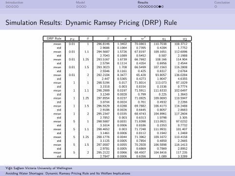
3. Using water data from Turkey, we conclude that cross-subsidization doesnot significantly lead to shortages. The average stock withoutcross-subsidization equals 296.8hm3 with a standard deviation of 3hm3.When the central planner cross-subsidizes agriculture, the average stockdrops only by about 4hm3, which corresponds to 1.35 percent and is aninsignificant decrease.




Agents

◮ Government (Water Utility): Manages water supply and sets the waterprices.

◮ Consumers: Households demand for tap water.

◮ Producers: Agriculture demand for irrigation water.

Details




Timeline of the Problem

1. The supplier observes how much water and bonds are saved from lastperiod.

2. The supplier chooses water prices before observing the shocks in thecurrent period.

3. During the period,* the current shocks are observed,* the supplier releases water given tap and irrigation water demands.* the supplier may bring more water from the external source.

4. The supplier saves the rest of water and net revenue (bonds) for nextperiod.




Benevolent Supplier

The supplier aims

◮ to maximize discounted expected lifetime utility of agents:

◮ subject to two constraints:

1. dynamic resource constraint

2. dynamic revenue constraint.

A water shortage occurs in any period, when the actual supply is less than thesum of aggregate demand for water and water savings.

w′(θ)︸︷︷︸

Savings

+ q1(p1; θo)

︸︷︷︸

Tap Water

+ q2(p2;θo)

︸︷︷︸

Irr Water

> S(w,θo)︸︷︷︸

Stock

; ∃ θo

.




Recursive Formulation of the SDP Problem

V (w, b, θ−1) =max Eθ|θ−1

{

(CS + δ Agr. Profits )1

1 + δ+ β V

(

w′, b′,θ)

}

∋ Dynamic Resource Constraint,

Dynamic Revenue Constraint

Notation:

◮ θ: a vector of exogenous stochastic shocks that may affect the environment

◮ Eθ|θ−1: expectation operator over the current shock vector, given last period’s

shock vector

◮ δ: degree of cross-subsidization

Details




Sectoral Water Prices

p1 = Inverse-Elasticity Rule + Marginal Value of Water + Marginal Cost

◮ Inverse-Elasticity Rule is the effect of the revenue constraint

◮ Marginal Value of Water is the shadow price due to scarcity

◮ Marginal Cost is the marginal production and transfer cost.

Details




Optimal prices with no cross-subsidization (δ = 1)

0.51

1.52

10 20 30 40 50 60 70

0.01

0.02

0.03

0.04

bond (b)

resource (w)

Tap

Pric

e

0.511.5220

4060

2

2.5

3

x 10−3

resource (w)

bond (b)

Irrig

atio

n P

rice




Optimal prices with cross-subsidization (δ = 1.5)

0.51

1.52

10 20 30 40 50 60 70

0.01

0.02

0.03

0.04

bond (b)

resource (w)

Tap

Pric

e

0.511.5220

4060

0

1

2

3

x 10−3

resource (w)

bond (b)

Irrig

atio

n P

rice




Comparative Dynamics

δ controls the degree of cross-subsidization

◮ If δ equals one, then the marginal rate of transformation betweenagricultural and households sectors equals one.

◮ If δ exceeds one, then the government values the agriculture’s profitsmore, so the agricultural sector will be cross-subsidized.

Question: How does cross-subsidization affect water prices?

◮ The irrigation price declines as the degree of cross-subsidization increases

◮ The tap water price increases as δ increases because of the revenueconstraint




External Water Demand

Suppose that marginal benefit of savings bonds is more than that of water,then two important results follow:

1. The demand for external water equals zero for at least one state of theshock vector.

2. The government’s demand for external water is positive only during awater shortage.




External Water Use

◮ If the price of the external supply is very high, then the government is notallowed to bring water from the external course.

◮ If the price of the external supply is very low, then water is essentiallyabundant: the government can use as much as it needs.

Question: How does the price of external water affect sectoral prices?

◮ Higher the price of the external supply makes it harder for the governmentto support the current stock with external water.

◮ The water prices increase to avoid shortages.




Figure: Geographical (GIS) Map of Cukurova Details

KARTALKAYA DAM

GAZ0ANTEP

0 80 16040 km

Legend

Dams

Other dams

Kartalkaya Dam

Rivers

Other rivers

Aksu River

Counties

Pazarcik County

Ceyhan Basin

River Basins

¯




Estimation Procedure

Data:

◮ Prices depends on the revenue constraint, but not on water scarcity.

◮ The ACP rule implies that price equals average cost.

◮ No bonds savings or no external water source.

Therefore, one can separate the two user groups to estimate the demand:

◮ Estimate the demand for tap and irrigation water

◮ Solve the SDP problem

Details




Simulation Results: Dynamic Ramsey Pricing (DRP) Rule

DRP Rule px δ S x w′ q1 q2

mean 0.01 1 296.8146 1.3402 70.0863 110.7038 108.3712std 2.9686 0.1064 0.7395 0.4284 1.7752

mean 0.01 1.1 294.5687 1.5726 67.8197 109.1651 112.6096std 2.7043 0.1089 0.5452 0.587 2.1988

mean 0.01 1.25 293.5167 1.6739 66.7692 108.166 114.904std 2.5794 0.1114 0.4354 0.6956 2.4544

mean 0.01 1.5 293.3023 1.708 66.5499 107.1563 116.2808std 2.5546 0.1161 0.425 0.8317 2.6764

mean 0.01 2 292.2104 8.3477 65.428 93.8057 136.0284std 2.447 0.5365 0.4273 1.9047 4.6355

mean 1 1 298.5194 0.017 71.8014 113.073 97.1029std 3.1518 0.003 0.8154 0.1536 0.7774

mean 1 1.1 298.2909 0.0197 71.5911 111.6333 102.6497std 3.1249 0.0028 0.799 0.225 1.3643

mean 1 1.25 297.8554 0.0237 71.0925 109.0693 110.5947std 3.0744 0.0024 0.761 0.4932 2.2266

mean 1 1.5 296.5529 0.0288 69.7882 106.4173 116.2488std 2.9186 0.0026 0.6445 0.8057 2.8683

mean 1 2 295.2347 0.0335 68.4743 104.8961 117.2604std 2.7852 0.003 0.6313 1.0798 3.305

mean 5 1 298.5987 0.0031 71.8398 113.0921 97.0232std 3.1614 0.0006 0.8186 0.1553 0.7732

mean 5 1.1 298.4652 0.003 71.7248 111.9931 101.407std 3.1461 0.0006 0.8112 0.1942 1.2469

mean 5 1.25 298.1776 0.0044 71.3962 109.1672 110.4158std 3.1125 0.0005 0.7854 0.4859 2.2665

mean 5 1.5 297.0587 0.0055 70.2928 106.5898 116.1413std 2.9781 0.0005 0.6869 0.7869 2.8952

mean 5 2 295.2122 0.0066 68.4507 104.8416 117.235std 2.7847 0.0006 0.6356 1.089 3.3289




Simulation Results: Dynamic Ramsey Pricing (DRP) Rule (cont.d)

DRP Rule px δ Welfare Cons. Surplus Agr. Profits Gov’t Revenue External Water Cost

mean 0.01 1 0.3914 0.3445 0.4382 0.1216 0std 0.0518 0.0725 0.0694 0.0786 0

mean 0.01 1.1 0.3945 0.2002 0.5711 0.137 0std 0.0565 0.0684 0.0652 0.086 0

mean 0.01 1.25 0.4098 0.1012 0.6566 0.1426 0std 0.0579 0.0955 0.0935 0.0844 0

mean 0.01 1.5 0.441 -0.0259 0.7523 0.1437 0std 0.0606 0.1264 0.1223 0.0851 0

mean 0.01 2 0.5449 -2.0081 1.8215 0.6836 0std 0.0715 0.3474 0.2206 0.0997 0

mean 1 1 0.3139 0.4983 0.1296 0.1876 0std 0.1128 0.2151 0.028 0.1721 0

mean 1 1.1 0.318 0.3731 0.268 0.2054 0std 0.1133 0.2145 0.054 0.1771 0

mean 1 1.25 0.3364 0.1401 0.4935 0.2327 0std 0.1166 0.2048 0.0674 0.1846 0

mean 1 1.5 0.375 -0.1415 0.7194 0.2593 0std 0.1193 0.2192 0.1214 0.1931 0

mean 1 2 0.4457 -0.3755 0.8563 0.2893 0std 0.1238 0.2424 0.1324 0.2155 0

mean 5 1 0.3128 0.498 0.1276 0.1888 0std 0.1151 0.2199 0.0285 0.1754 0

mean 5 1.1 0.3154 0.4034 0.2355 0.2014 0std 0.1141 0.2191 0.0509 0.1788 0

mean 5 1.25 0.3392 0.15 0.4906 0.2261 0std 0.1177 0.2106 0.0853 0.1857 0

mean 5 1.5 0.376 -0.1173 0.7048 0.2552 0std 0.1199 0.2192 0.1182 0.1936 0

mean 5 2 0.4433 -0.386 0.858 0.2948 0std 0.1261 0.2454 0.1295 0.2213 0




Where To Now?

1. Application: This model can easily be applied to differentdatasets/regions.

2. Policy Evaluation: Using the Euler equation for optimal prices, we canindeed reverse engineer how much weight suppliers put on resource andrevenue constraints? This could be done using Non-LS or GMMtechniques.

3. Water Markets: We could endogenize the marginal cost of the externalwater and hypothesize to what extent a market for water could help avoidshortages in this setup.

4. LPMs in Resource Management: We could focus on the effect ofshortages on agriculture using Lower-Partial Moments: Roseta-Palma andSaglam (2014) currently under progress.




Consumers: Households

◮ Consumers spend their fixed income on tap water and a composite good.

◮ Quasi-linear preferences for the utility function:

◮ Tap water may have different uses, such as drinking (price-non-responsive)and non-drinking (price-responsive) components.

U(q1, y;θ) = U(q1 − q1;θ) + y

◮ Utility maximization problem leads to the total demand for tap water.

max<q1>

U(q1 − q1;θ)− p1 q1

⇒ U ′(q1 − q1;θ) = p1




Producers: Agriculture

◮ Producers are identical farmers in a perfectly competitive output market.

◮ Mixed-Choice Problem:

* Farmers choose which crop to produce.

* Having chosen the crop, the farmers then decide how much land to allocate.

Π =max (Π1,Π2, . . . ,ΠN ,ΠN+1) , where

Πc = max<ℓc,q2,c>

pFc Fc(ℓc, q2,c)− p2 q2,c + µc ℓc; ∀c = 1, . . . , N

ΠN+1 =µN+1ℓc

∋ ℓc ≤ ℓ = 1

◮ Partial Equilibrium with iid shocks across farmers and time




Producers: Agriculture Back

Given a distribution of the shocks, one can calculate

◮ Probability of choosing crop c: Pr(ac = 1 | p2,θ)

◮ Expected total profit by agriculture: EθΠ(p2; θ)

◮ Expected demand for irrigation water: Eθq2(p2;θ)




Government Constraints

1. Dynamic Resource Constraint: Intertemporal resource allocation of water

w′(θ) + q1(p1;θ) + q2(p2;θ) ≤ S(w,θ) + x(θ); ∀ θ, (1)

Notation:

◮ w′(θ): water savings for next period

◮ q1(p1;θ), q2(p2;θ): demand for tap and irrigation water

◮ S(w,θ): stock of water in the reservoir

◮ x(θ): external water demand through desalination technology ornetworking.




Government Constraints

2. Dynamic Revenue Constraint:

b′(θ) + px x(θ) ≤(p1 − c1) q1(p1;θ) + (p2 − c2) q2(p2; θ)+ (2)

R b− τ ; ∀ θ,

Notation:

◮ b′(θ): bond savings for next period

◮ px x(θ): cost of external water purchase

◮ R b: return on bond from last period

◮ c1, c2: marginal cost of production for tap and irrigation water

◮ τ : fixed cost of water production




Dynamic Ramsey Pricing Back

V (w, b, θ−1) = max<p,w′(θ),b′(θ),x(θ)>

Eθ|θ−1

{

U [q1(p1; θ)] − p1 q1(p1; θ) + δ Π(p2; θ)

1 + δ

}

+

β Eθ|θ−1

[

V(

w′(θ), b′(θ), θ

)]

∋ w′(θ) + q1(p1; θ) + q2(p2; θ) ≤ S(w, θ) + x(θ); ∀ θ,

b′(θ) + px x(θ) ≤ (p1 − c1) q1(p1; θ) + (p2 − c2) q2(p2; θ) + R b − τ ; ∀ θ,

q1(p1; θ), q2(p2; θ), w′(θ), x(θ) ≥ 0




Estimation: Irrigation Water Back

◮ Tap water price:

p1 =

[Eθ(µ(θ)− 1/(1 + δ)) (−q1(p1;θ))

Eθµ(θ) ∂q1(p1;θ)/∂p1

]

+

Eθ(λ(θ) ∂q1(p1;θ)/∂p1)

Eθ(µ(θ) ∂q1(p1;θ)/∂p1)+ c1.

◮ Irrigation water price:

p2 =

[(δ/(1 + δ)) ∂EθΠ(p2;θ)/∂p2 − Eθµ(θ) q2(p2;θ)

Eθµ(θ) ∂q2(p2;θ)/∂p2

]

+

Eθλ(θ) ∂q2(p2;θ)/∂p2Eθµ(θ) ∂q2(p2;θ)/∂p2

+ c2.




Data

◮ Data collection:

* Water flows data from the State Water Works

* Irrigation price and land allocation data from the local water userassociations

* Tap price, quantity, and water sanitation data from the municipality

* Climatic variables from Turkish Meteorological Institute

◮ Monthly time-series data from 01/1984 to 08/2007

◮ Irrigation prices and land allocation are yearly data from 1984 to 2007.




Figure: Reservoir Flows

4

6

8

10

1 2 3 4 5 6 7 8 9 10 11 12Month

Tap

Wat

er U

se

0

10

20

30

40

50

60

1 2 3 4 5 6 7 8 9 10 11 12Month

Irrig

atio

n W

ater

Use

0

50

100

150

200

250

1 2 3 4 5 6 7 8 9 10 11 12Month

Flo

od C

ontr

ol U

se

50

100

150

200

250

300

1 2 3 4 5 6 7 8 9 10 11 12Month

Inflo

ws




Figure: Crop Composition

1985 1990 1995 2000 20050

10

20

30

40

50

60

70

80

90

100

Year

Per

cent

Lan

d A

lloca

tion

Crop Composition

CottonMaizeWheatSugarbeetFallow




Figure: Tap Price vs Revenue: Inelastic demand for tap water.

01/2000 01/2002 01/2004 01/2006 01/2008

1.5

2

2.5

3

3.5

Time

Var

iabl

es

Tap Water (m3) vs. Price (per 100 m3)

Tap Water UseTap Water Price

01/2000 01/2002 01/2004 01/2006 01/2008

0.02

0.03

0.04

0.05

0.06

Time

Var

iabl

es

Revenue vs. Price

RevenueTap Water Price




Figure: Irrigation Prices

2

4

6

8

10

12

14Irrigation Water Prices

Year

Pric

es

CottonMaizeSugar BeetWheat

1985 1990 1995 2000 2005

0.04

0.06

0.08

0.1

0.12

0.14

0.16

Irrigation Water Prices (1994=100)

Year

Rea

l Pric

es




Figure: Irrigation Water Demand Back

0 1 2 3100

120

140

160

180Irrigation Water Demand vs. Irrigation Price

Irr Price

Irr

Wat

er

LowMidHigh

0 1 2 30

0.2

0.4

0.6

0.8Elasticity of Irriation Demand

Irr Price

Ela

stic

ity

LowMidHigh

0.5 1 1.5 2 2.50

20

40

60

80

100

Irr Price

Per

cent

age

Percent Land Allocations vs. Irrigation Price (High)

CottonMaizeWheatSugarbeetFallow

Figure: Irrigation Water DemandYigit Saglam Victoria University of Wellington



Solving the SDP Problem

◮ I aggregated the flows data to annual frequency to have a single valuefunction:

* Estimate the Tobit model for the water release for flood control,* Estimate AR(1) process for the crop prices,* Fit the gamma distribution for the annual inflows,* Use Chebychev Polynomials to approximate the value function.

◮ Solve the SDP problem for different values of δ and px.

◮ Simulate the economy for 100 years for 5, 000 times across δ and px underthe ACP and DRP rules.

◮ Compute the summary statistics for key variables in each case.




Simulation Results: Average-Cost Pricing (ACP) Rule

ACP Rule px δ S x w′ q1 q2

mean 0.01 1 233.6464 15.2873 6.1326 95.3225 147.4785std 4.555 1.7694 2.84 0 0.0305

mean 0.01 1.1 233.6464 15.2873 6.1326 95.3225 147.4785std 4.555 1.7694 2.84 0 0.0305

mean 0.01 1.25 233.6464 15.2873 6.1326 95.3225 147.4785std 4.555 1.7694 2.84 0 0.0305

mean 0.01 1.5 233.6464 15.2873 6.1326 95.3225 147.4785std 4.555 1.7694 2.84 0 0.0305

mean 0.01 2 233.6464 15.2873 6.1326 95.3225 147.4785std 4.555 1.7694 2.84 0 0.0305

mean 1 1 233.6464 15.2873 6.1326 95.3225 147.4785std 4.555 1.7694 2.84 0 0.0305

mean 1 1.1 233.6464 15.2873 6.1326 95.3225 147.4785std 4.555 1.7694 2.84 0 0.0305

mean 1 1.25 233.6464 15.2873 6.1326 95.3225 147.4785std 4.555 1.7694 2.84 0 0.0305

mean 1 1.5 233.6464 15.2873 6.1326 95.3225 147.4785std 4.555 1.7694 2.84 0 0.0305

mean 1 2 233.6464 15.2873 6.1326 95.3225 147.4785std 4.555 1.7694 2.84 0 0.0305

mean 5 1 233.6464 15.2873 6.1326 95.3225 147.4785std 4.555 1.7694 2.84 0 0.0305

mean 5 1.1 233.6464 15.2873 6.1326 95.3225 147.4785std 4.555 1.7694 2.84 0 0.0305

mean 5 1.25 233.6464 15.2873 6.1326 95.3225 147.4785std 4.555 1.7694 2.84 0 0.0305

mean 5 1.5 233.6464 15.2873 6.1326 95.3225 147.4785std 4.555 1.7694 2.84 0 0.0305

mean 5 2 233.6464 15.2873 6.1326 95.3225 147.4785std 4.555 1.7694 2.84 0 0.0305




Simulation Results: Average-Cost Pricing (ACP) Rule (cont.d) Back

ACP Rule px δ Welfare Cons. Surplus Agr. Profits Gov’t Revenue External Water Cost

mean 0.01 1 -0.7006 -1.7449 2.476 0.0001 1.0662std 0.4061 0 0.083 0.0004 0.4159

mean 0.01 1.1 -0.6001 -1.7449 2.476 0.0001 1.0662std 0.4057 0 0.083 0.0004 0.4159

mean 0.01 1.25 -0.4661 -1.7449 2.476 0.0001 1.0662std 0.4052 0 0.083 0.0004 0.4159

mean 0.01 1.5 -0.2785 -1.7449 2.476 0.0001 1.0662std 0.4046 0 0.083 0.0004 0.4159

mean 0.01 2 0.0028 -1.7449 2.476 0.0001 1.0662std 0.4037 0 0.083 0.0004 0.4159

mean 1 1 -106.2611 -1.7449 2.476 0.0001 106.6266std 41.5815 0 0.083 0.0004 41.5933

mean 1 1.1 -106.1606 -1.7449 2.476 0.0001 106.6266std 41.5809 0 0.083 0.0004 41.5933

mean 1 1.25 -106.0266 -1.7449 2.476 0.0001 106.6266std 41.5802 0 0.083 0.0004 41.5933

mean 1 1.5 -105.839 -1.7449 2.476 0.0001 106.6266std 41.5792 0 0.083 0.0004 41.5933

mean 1 2 -105.5576 -1.7449 2.476 0.0001 106.6266std 41.5776 0 0.083 0.0004 41.5933

mean 5 1 -532.7678 -1.7449 2.476 0.0001 533.1334std 207.9546 0 0.083 0.0004 207.9664

mean 5 1.1 -532.6673 -1.7449 2.476 0.0001 533.1334std 207.9541 0 0.083 0.0004 207.9664

mean 5 1.25 -532.5333 -1.7449 2.476 0.0001 533.1334std 207.9533 0 0.083 0.0004 207.9664

mean 5 1.5 -532.3457 -1.7449 2.476 0.0001 533.1334std 207.9523 0 0.083 0.0004 207.9664

mean 5 2 -532.0644 -1.7449 2.476 0.0001 533.1334std 207.9507 0 0.083 0.0004 207.9664



Date post:	06-Mar-2019
Category:	Documents
Upload:	doanminh
View:	213 times
Download:	0 times

AvoidingWaterShortages ... Story/SDN...Introduction Model Results Conclusion AvoidingWaterShortages:...

Documents