554
Lecture Notes Financial Econometrics Professor Doron E. Avramov Hebrew University of Jerusalem ' Prof . Doron Avramov Financial Econometrics 1
| Date post: | 08-Aug-2018 |
| Category: |
Documents |
| Upload: | alvaro-mamani-machaca |
| View: | 266 times |
| Download: | 8 times |

8/22/2019 Avramov Doron Financial Econometrics
http://slidepdf.com/reader/full/avramov-doron-financial-econometrics 1/553
Lecture Notes
Financial Econometrics
Professor Doron E. Avramov
Hebrew University of Jerusalem
'Prof. Doron Avramov
Financial Econometrics1
8/22/2019 Avramov Doron Financial Econometrics
http://slidepdf.com/reader/full/avramov-doron-financial-econometrics 2/553
Syllabus: Motivation• Why do we need a course in financial
econometrics?
• The past few decades have been characterized
by an extraordinary growth in the use of
quantitative methods in financial markets inanalyzing various asset classes; be it equities,
fixed income instruments, commodities, or
derivative securities.
'Prof. Doron Avramov
Financial Econometrics2

8/22/2019 Avramov Doron Financial Econometrics
http://slidepdf.com/reader/full/avramov-doron-financial-econometrics 3/553
Syllabus: MotivationFinancial market participants, both academics
and practitioners, have been routinely using
advanced econometric techniques in a host of
applications including portfolio management,
risk management, modeling volatility,understanding pivotal issues in corporate
finance, asset pricing, interest rate modeling, as
well as regulatory purposes.
'Prof. Doron Avramov
Financial Econometrics3

8/22/2019 Avramov Doron Financial Econometrics
http://slidepdf.com/reader/full/avramov-doron-financial-econometrics 4/553
Syllabus: Objectives• This course attempts to provide a fairly deep
understanding of topical issues in asset pricing
and deliver econometric methods in which to
develop research agenda in financial economics.
•The course targets advanced master level and
PhD level students in finance and economics.
'Prof. Doron Avramov
Financial Econometrics4

8/22/2019 Avramov Doron Financial Econometrics
http://slidepdf.com/reader/full/avramov-doron-financial-econometrics 5/553
Syllabus: Prerequisite• I will assume some prior exposure to matrix
algebra, distribution theory, Ordinary Least
Squares, and Maximum Likelihood
Estimation.
• I will also assume you have some skills in
computer programing beyond Excel.
Suggested packages include MATLAB,STATA, SAS, R, etc.
'Prof. Doron Avramov
Financial Econometrics5

8/22/2019 Avramov Doron Financial Econometrics
http://slidepdf.com/reader/full/avramov-doron-financial-econometrics 6/553
Syllabus: Topics to be CoveredOverview:
Matrix algebra
Regression analysisLaw of iterated expectations
Variance decomposition
Taylor approximationDistribution theory
Hypothesis testing
OLS
MLE
'Prof. Doron Avramov
Financial Econometrics6

8/22/2019 Avramov Doron Financial Econometrics
http://slidepdf.com/reader/full/avramov-doron-financial-econometrics 7/553
Syllabus: Topics to be CoveredTesting asset pricing models including the CAPM
and multi factor models: Time series analysis.
The econometrics of the mean variance frontier
Estimating expected returns
Estimating the covariance matrix of stock returns.
Forming mean variance efficient portfolio, the
Global Minimum Volatility Portfolio, and the
minimum Tracking Error Volatility Portfolio.'Prof. Doron Avramov
Financial Econometrics7

8/22/2019 Avramov Doron Financial Econometrics
http://slidepdf.com/reader/full/avramov-doron-financial-econometrics 8/553
Syllabus: Topics to be CoveredThe Sharpe ratio: estimation and distribution
The Delta method
The Black-Litterman approach for estimating expected
returns.
Principal component analysis.
'Prof. Doron Avramov
Financial Econometrics8
8/22/2019 Avramov Doron Financial Econometrics
http://slidepdf.com/reader/full/avramov-doron-financial-econometrics 9/553
Syllabus: Topics to be CoveredRisk management and the downside risk measures:
value at risk, shortfall probability, expectedshortfall, target semi-variance, downside beta, and
drawdown.
Option pricing: testing the validity of the B&S
formula
Model verification based on failure rates
'Prof. Doron Avramov
Financial Econometrics9

8/22/2019 Avramov Doron Financial Econometrics
http://slidepdf.com/reader/full/avramov-doron-financial-econometrics 10/553
Syllabus: Topics to beCoveredVariance ratio tests
Predicting asset returns using time series regressions
The econometrics of back-testing
Understanding time varying volatility models
including ARCH, GARCH, EGARCH, stochastic
volatility, implied volatility, and realized volatility
'Prof. Doron Avramov
Financial Econometrics10

8/22/2019 Avramov Doron Financial Econometrics
http://slidepdf.com/reader/full/avramov-doron-financial-econometrics 11/553
Syllabus: Grade Components• Assignments (35%): there will be three problem sets
during the term. You can form study groups to prepare
the assignments with up to four students per group.
•Class Participation (15%) - Attending AT LEAST 80%
of the sessions is mandatory.•Take-home final exam (50%): based on class material,
handouts, assignments, and readings.
'Prof. Doron Avramov
Financial Econometrics11

8/22/2019 Avramov Doron Financial Econometrics
http://slidepdf.com/reader/full/avramov-doron-financial-econometrics 12/553
Let us StartThis session is mostly an overview. Major contents:
• Why do we need a course in financial econometrics?• Normal, Bivariate normal, and multivariate normal
densities
• The Chi-squared, F, and Student t distributions
• Regression analysis
• Basic rules and operations applied to matrices
• Iterated expectations and variance decomposition'Prof. Doron Avramov
Financial Econometrics12

8/22/2019 Avramov Doron Financial Econometrics
http://slidepdf.com/reader/full/avramov-doron-financial-econometrics 13/553
Financial EconometricsIn previous courses in finance and economics you
mastered the concept of the efficient frontier.
A portfolio lying on the frontier is the highest
expected return portfolio for a given volatility target.
Or it is the lowest volatility portfolio for a given
expected return target.
'Prof. Doron Avramov
Financial Econometrics13

8/22/2019 Avramov Doron Financial Econometrics
http://slidepdf.com/reader/full/avramov-doron-financial-econometrics 14/553
Plotting the Efficient Frontier
'Prof. Doron Avramov
Financial Econometrics14

8/22/2019 Avramov Doron Financial Econometrics
http://slidepdf.com/reader/full/avramov-doron-financial-econometrics 15/553
However, how could you Practically Form
an Efficient Portfolio?
• Problem: there are TOO many parameters to estimate.
For instance, investing in ten assets requires:
which is about ten estimates for expected return, ten for volatility, and 45 for covariances/correlations.
Overall, 65 estimates are required. That is a lot!!!
10
2
1
.
.
µ
µ
µ
2
1010,1
2
22,1
10,1
2
,
1
σ σ
σ σ
σ σ
KKKKK
KKKKKKKK
KKKKK
KKKKK
'Prof. Doron Avramov
Financial Econometrics15

8/22/2019 Avramov Doron Financial Econometrics
http://slidepdf.com/reader/full/avramov-doron-financial-econometrics 16/553
More generally, if there are N investable assets, you need:
• N estimates for the means,
• N estimates for the volatilities,
• 0.5N(N-1) estimates for correlations.
Overall: 2N+0.5N(N-1) estimates are required!
Mean, volatility, and correlation estimates are noisy
as reflected through their standard errors.
'Prof. Doron Avramov
Financial Econometrics16

8/22/2019 Avramov Doron Financial Econometrics
http://slidepdf.com/reader/full/avramov-doron-financial-econometrics 17/553
• The volatility estimate is less noisy than the mean.
• I will later show that the standard error of the volatilityestimate is lower than that of mean return.
• We have T asset return observations:
•The sample mean and volatility are given by
T R R R R KKK321 ,,
( )
1
ˆ
2
1
−
−= ∑=
T
R RT
t t σ Less noisy
'Prof. Doron Avramov
Financial Econometrics17
T
R R
T
t t ∑ == 1
Sample Mean and Volatility

8/22/2019 Avramov Doron Financial Econometrics
http://slidepdf.com/reader/full/avramov-doron-financial-econometrics 18/553
Estimation Methods
• One of the ideas here is to introduce robust methods
in which to estimate the comprehensive set of
parameters.
• We will discuss asset pricing models and the Black
Litterman approach for estimating expected returns.• We will further introduce several methods for
estimating the large-scale covariance matrix of asset
returns.
'Prof. Doron Avramov
Financial Econometrics18

8/22/2019 Avramov Doron Financial Econometrics
http://slidepdf.com/reader/full/avramov-doron-financial-econometrics 19/553
Mean-Variance vs. Down
Side Risk
•We will comprehensively cover topics in meanvariance analysis.
•We will also depart from the mean variance
paradigm and consider down side risk measuresto form as well as evaluate investment strategies.
• Why do we need to resort to down side risk?
'Prof. Doron Avramov
Financial Econometrics19

8/22/2019 Avramov Doron Financial Econometrics
http://slidepdf.com/reader/full/avramov-doron-financial-econometrics 20/553
Down Side Risk
• For one, investors often care more about the
down side of investment payoffs than the upside
potential.
•The practice of risk management as well as
regulations of financial institutions are typicallyabout downside risk – such as targeting VaR,
shortfall probability, and expected shortfall.
•Moreover, there is a major weakness embedded
in the mean variance paradigm.
'Prof. Doron AvramovFinancial Econometrics
20

8/22/2019 Avramov Doron Financial Econometrics
http://slidepdf.com/reader/full/avramov-doron-financial-econometrics 21/553
Drawback in the Mean-Variance Setup
• To illustrate, consider two stocks, A and B, with
correlation coefficient smaller than unity.
•There are five states of nature in the economy.
•Returns in the various states are described on the
next page.
'Prof. Doron AvramovFinancial Econometrics
21

8/22/2019 Avramov Doron Financial Econometrics
http://slidepdf.com/reader/full/avramov-doron-financial-econometrics 22/553
• Stock A dominates stock B in every state of nature.
• Nevertheless, a mean-variance investor may consider
stock B because it can reduce the portfolio’s volatility.
• Investment criteria based on down size risk measurescould get around this weakness.
S5S4S3S2S1
20.05%10.50%15.00%8.25%5.00%A3.01%3.10%2.95%2.90%3.05%B
'Prof. Doron AvramovFinancial Econometrics
22
Drawback in Mean-Variance

8/22/2019 Avramov Doron Financial Econometrics
http://slidepdf.com/reader/full/avramov-doron-financial-econometrics 23/553
The Normal Distribution• In various applications in finance and economics, a
common assumption is that quantities of interests, such
as asset returns, economic growth, dividend growth,
interest rates, etc., are normally (or log-normally)
distributed.
• The normality assumption is primarily done for
analytical tractability.
• The normal distribution is symmetric.
• It is characterized by the mean and the variance.
'Prof. Doron AvramovFinancial Econometrics
23

8/22/2019 Avramov Doron Financial Econometrics
http://slidepdf.com/reader/full/avramov-doron-financial-econometrics 24/553
Confidence Level Normality suggests that deviation of 2 SD away from
the mean creates an 80% range (from -32% to 48%) for
the realized return with 95% confidence level.
'Prof. Doron AvramovFinancial Econometrics
24

8/22/2019 Avramov Doron Financial Econometrics
http://slidepdf.com/reader/full/avramov-doron-financial-econometrics 25/553
Dispersion around the Mean
• Assuming that x is a zero mean random variable.
•As the distribution takes the form:
• When is small, the distribution is concentrated and
vice versa.
2,0~ σ N x
'Prof. Doron AvramovFinancial Econometrics
25

8/22/2019 Avramov Doron Financial Econometrics
http://slidepdf.com/reader/full/avramov-doron-financial-econometrics 26/553
Probability Distribution Function
• The Probability Density Function (pdf) of the normal
distribution is:
• If then:
• The Cumulative Density Function (CDF), which is the
integral of the pdf, is 50% at that point.
( )
−−=2
2
2 2
1exp
2
1)(
σ
µ
πσ
r r pdf
==
r µ
σ 1
π 2
1)( =r pdf
'Prof. Doron AvramovFinancial Econometrics
26

8/22/2019 Avramov Doron Financial Econometrics
http://slidepdf.com/reader/full/avramov-doron-financial-econometrics 27/553
Normally Distributed Return•Assume that the US excess rate of return on the
market portfolio is normally distributed with annual
mean (equity premium) and volatility given by 8% and20%, respectively.
•That is to say that with a nontrivial probability theactual excess annual market return can be negative.
See figures on the next page.
'Prof. Doron AvramovFinancial Econometrics
27

8/22/2019 Avramov Doron Financial Econometrics
http://slidepdf.com/reader/full/avramov-doron-financial-econometrics 28/553
Confidence Intervals for Annual Excess
Return on the Market
The probability that the realization is negative
%99)2.0308.02.0308.0(Pr
%95)2.0208.02.0208.0(Pr
%68)2.008.02.008.0(Pr
=×+<<×−
=×+<<×−
=+<<−
Rob
Rob
Rob
'Prof. Doron AvramovFinancial Econometrics
28
%4.34)4.0(Pr
2.0
08.00
2.0
08.0Pr )0(Pr
=−<=
−<
−=<
z ob
Rob Rob
8/22/2019 Avramov Doron Financial Econometrics
http://slidepdf.com/reader/full/avramov-doron-financial-econometrics 29/553
Higher Moments• Skewness – the third moment - is zero.
• Kurtosis – the fourth moment – is three.
• Odd moments are all zero.
• Even moments are (often complex) functions of themean and the variance.
•In the next slides, skewness and kurtosis are presented
for other distribution functions.
'Prof. Doron AvramovFinancial Econometrics
29

8/22/2019 Avramov Doron Financial Econometrics
http://slidepdf.com/reader/full/avramov-doron-financial-econometrics 30/553
Skewness• The skewness can be negative (left tail) or
positive (right tail).
'Prof. Doron AvramovFinancial Econometrics
30
Kurtosis

8/22/2019 Avramov Doron Financial Econometrics
http://slidepdf.com/reader/full/avramov-doron-financial-econometrics 31/553
Kurtosis
'Prof. Doron AvramovFinancial Econometrics
31
• Mesokurtic - A term used in a statistical context where the
kurtosis of a distribution is similar, or identical, to the
kurtosis of a normally distributed data set.

8/22/2019 Avramov Doron Financial Econometrics
http://slidepdf.com/reader/full/avramov-doron-financial-econometrics 32/553
•
•Positive skewness means non-zero probability for large payoffs.
• Kurtosis is a measure for how tick the distribution’s tails are.
• When is the skewness zero? In symmetric distributions.
'Prof. Doron AvramovFinancial Econometrics
32
The Essence of Skewness and
Kurtosis

8/22/2019 Avramov Doron Financial Econometrics
http://slidepdf.com/reader/full/avramov-doron-financial-econometrics 33/553
Bivariate Normal Distribution
• Bivariate normal:
• The marginal densities of x and y are
• What is the distribution of y if x is known?
22
2
,
,,~
y xy
xy x
y
x N
y
x
σ σ
σ σ
µ
µ
(( )[ ]2
2
,~
,~
y y
x x
N y
N x
σ µ
σ µ
'Prof. Doron AvramovFinancial Econometrics
33

8/22/2019 Avramov Doron Financial Econometrics
http://slidepdf.com/reader/full/avramov-doron-financial-econometrics 34/553
Conditional Distribution
• Conditional distribution:
always non-negative• When the correlation between x and y is positive
and - then the conditional expectation ishigher than the unconditional one.
( )
−−+ 2
2
22
,~ x
xy y x
x
xy y x N x y
σ σ σ µ
σ σ µ
x x µ >
'Prof. Doron AvramovFinancial Econometrics
34

8/22/2019 Avramov Doron Financial Econometrics
http://slidepdf.com/reader/full/avramov-doron-financial-econometrics 35/553
Conditional Moments• If we have no information about x, or if x and y are
uncorrelated, then the conditional and unconditional
expected return of y are identical.• Otherwise, the expected return of y is .
• If , then:
Here, the realization of x does not say anything about y.
0= xyσ
x yµ
y
x
xy
y x y σ σ
σ σ σ =−=
2
2
2
'Prof. Doron AvramovFinancial Econometrics
35

8/22/2019 Avramov Doron Financial Econometrics
http://slidepdf.com/reader/full/avramov-doron-financial-econometrics 36/553
Conditional Standard Deviation
• Developing the conditional standard deviation further:
• When goodness of fit is higher the conditional standarddeviation is lower.
( )2
22
2
2
2
2
2 11 R y
y x
xy
y
x
xy
y x y −=
⋅
−=−= σ
σ σ
σ σ
σ
σ σ σ
'Prof. Doron AvramovFinancial Econometrics
36
M lti i t N l

8/22/2019 Avramov Doron Financial Econometrics
http://slidepdf.com/reader/full/avramov-doron-financial-econometrics 37/553
• Define Z=AX+B.
( )mmm
m
m N
x
x
x
X ××× ∑
= ,~
.
. 1
2
1
1 µ
'Prof. Doron AvramovFinancial Econometrics
37
Multivariate Normal

8/22/2019 Avramov Doron Financial Econometrics
http://slidepdf.com/reader/full/avramov-doron-financial-econometrics 38/553
• Let us make some transformations to end up with
N (0,I):
( )
( )( ) ),0(~
),0(~
),(~
11
2
1'
'11
'
1111
I N B A Z A A
A A N B A Z
A A B A N B X A Z
nmmnnmmmmn
nmmmmnnmmn
nmmmmnnmmnnmmn
×××
−
×××
×××⋅××
×××××××××
−−∑
∑+−
∑++⋅=
µ
µ
µ
'Prof. Doron AvramovFinancial Econometrics
38
Multivariate Normal

8/22/2019 Avramov Doron Financial Econometrics
http://slidepdf.com/reader/full/avramov-doron-financial-econometrics 39/553
Multivariate Normal
• Consider an N -vector or returns which is normally
distributed:
• Then:
• What does mean? A few rules:
( ) N N N N N R ××× ∑,~ 11 µ
( )
( ) ( ) I N R
N R
,0~
,0~
2
1
µ
µ
−∑
∑−
−
2
1−
∑
I =∑⋅∑
∑=∑⋅∑
∑=∑⋅∑
−
−−−
2
1
2
1
2
1
2
1
12
1
2
1
'Prof. Doron AvramovFinancial Econometrics
39

8/22/2019 Avramov Doron Financial Econometrics
http://slidepdf.com/reader/full/avramov-doron-financial-econometrics 40/553
• If X 1~N(0,1) then
• If X 1~N(0,1), X 2~N (0,1) & then:
( )2~ 222
21 χ X X +
21 X X ⊥
'Prof. Doron AvramovFinancial Econometrics
40
The Chi-Squared Distribution
( )1~ 22
1 χ X

8/22/2019 Avramov Doron Financial Econometrics
http://slidepdf.com/reader/full/avramov-doron-financial-econometrics 41/553
• Moreover if
then
( )
( )
21
2
2
2
1
~
~
X X
n X
m X
⊥
χ
χ
( )nm X X ++ 221 ~ χ
'Prof. Doron AvramovFinancial Econometrics
41
More about the Chi-Squared
The F Distribution

8/22/2019 Avramov Doron Financial Econometrics
http://slidepdf.com/reader/full/avramov-doron-financial-econometrics 42/553
•Gibbons, Ross & Shanken (GRS) designated a finite
sample asset pricing test that has the F - Distribution.
•If
•Then
),(~2
1
nm F
n X m
X
A =
( )( )
21
2
2
21
~
~
X X
n X
m X
⊥
χ
χ
'Prof. Doron AvramovFinancial Econometrics
42
The F Distribution
The Student’s t Distribution

8/22/2019 Avramov Doron Financial Econometrics
http://slidepdf.com/reader/full/avramov-doron-financial-econometrics 43/553
The Student s t Distribution
'Prof. Doron AvramovFinancial Econometrics
43
The t Distribution
8/22/2019 Avramov Doron Financial Econometrics
http://slidepdf.com/reader/full/avramov-doron-financial-econometrics 44/553
• The pdf of student-t is given by:
• Where is beta function and is a number of
degrees of freedom
The t Distribution
'Prof. Doron AvramovFinancial Econometrics
44
( )( )
2
12
121,2
1,
+−
+⋅
⋅=
v
v x
v Bvv x f
( )ba B , 1≥v
The t Distribution

8/22/2019 Avramov Doron Financial Econometrics
http://slidepdf.com/reader/full/avramov-doron-financial-econometrics 45/553
• As noted earlier, is a sample of length T of
stock returns which are normally distributed.
• The sample mean and variance are
• The resulting t -value which has the t distribution with T-1
d.o.f is
The t Distribution
'Prof. Doron AvramovFinancial Econometrics
45
T r r r ,,, 21 K
T
r r
r
T K+
=
1
and ( )∑= −−=
T
t t r r T s 1
22
1
1
1−−=T
sr t µ
The t Distribution

8/22/2019 Avramov Doron Financial Econometrics
http://slidepdf.com/reader/full/avramov-doron-financial-econometrics 46/553
• The t -distribution is the sampling distribution of the t -value
when the sample consist of independent and identically
distributed observations from a normally distributed population.
• It is obtained by dividing a normally distributed random variable
by a square root of a Chi-squared distributed random variable
when both random variables are independent.
• Indeed, later we will show that when returns are normally
distributed the sample mean and variance are independent.
The t Distribution
'Prof. Doron AvramovFinancial Econometrics
46
R i A l i

8/22/2019 Avramov Doron Financial Econometrics
http://slidepdf.com/reader/full/avramov-doron-financial-econometrics 47/553
Regression Analysis• Various applications in corporate finance and asset
pricing require the implementation of a regression
analysis.• We will estimate regressions using matrix notation.
• For instance, consider the time series regression
t t t t Z Z R ε β β α +++= 2211 T ,2,1, KK=∀
'Prof. Doron AvramovFinancial Econometrics
47
R iti th t i t i f

8/22/2019 Avramov Doron Financial Econometrics
http://slidepdf.com/reader/full/avramov-doron-financial-econometrics 48/553
• Rewriting the system in a matrix form:
yields
• We will derive regression coefficients and their standard
errors using OLS, MLE, and Method of Moments.
=×
21
2221
1211
3
,,1
.
.
,,1
,,1
T T
T
Z Z
Z Z
Z Z
X
=×
2
113
β β
α
γ
11331 ×××× += T T T X R ε γ
=×
T
T
ε
ε
ε
ε ..
2
1
1
'Prof. Doron AvramovFinancial Econometrics
48
=×
T
T
R
R
R
R..
2
1
1

8/22/2019 Avramov Doron Financial Econometrics
http://slidepdf.com/reader/full/avramov-doron-financial-econometrics 49/553
Vectors and Matrices: some Rules
• If A is a row vector:
• Then the transpose of A is a column vector:
• The identity matrix satisfies
[ ]t t aaa A 112,111 ,K=×
=×
1
21
11
1
.
.'
t
t
a
a
a
A
B I B B I =⋅=⋅
'Prof. Doron AvramovFinancial Econometrics
49
M l i li i f M i

8/22/2019 Avramov Doron Financial Econometrics
http://slidepdf.com/reader/full/avramov-doron-financial-econometrics 50/553
Multiplication of Matrices:
,
The inverse of the matrix A is A-1 which satisfies:
=×
22,21
12,11
22aa
aa A
=×
22,12
21,11
22'aa
aa A
=×
22,21
12,11
22bb
bb B
++
++=××
22221221,21221121
22121211,21121111
2222babababa
babababa B A
==−
×× 1,0
0,11
2222 I A A
111)(
'')'(
−−− =
=
A B AB
A B AB
'Prof. Doron AvramovFinancial Econometrics
50

8/22/2019 Avramov Doron Financial Econometrics
http://slidepdf.com/reader/full/avramov-doron-financial-econometrics 51/553
Solving Large Scale Linear Equations:
• Of course, A has to be a square invertible matrix.
b
b X A mmmm
1
11
−
×××
=
=
'Prof. Doron AvramovFinancial Econometrics
51
Linear Independence and Norm

8/22/2019 Avramov Doron Financial Econometrics
http://slidepdf.com/reader/full/avramov-doron-financial-econometrics 52/553
Linear Independence and Norm
• The vectors are linearly independent if there
does not exists scalars such that
• The norm of a vector V is
'Prof. Doron AvramovFinancial Econometrics
52
N V V ,,1 K
N cc ,,1 K
unless
V cV cV c N N 02211 =+++ K
021 === N ccc K
V V V '=
A Positive Definite Matrix

8/22/2019 Avramov Doron Financial Econometrics
http://slidepdf.com/reader/full/avramov-doron-financial-econometrics 53/553
A Positive Definite Matrix
• An matrix is called positive definite if
for any nonzero vector V.
• A non positive definite matrix cannot be inverted and
its determinant is zero.
'Prof. Doron AvramovFinancial Econometrics
53
N N × ∑
0' 11 >⋅∑⋅ ××× N N N N V V
The Trace of a Matrix
8/22/2019 Avramov Doron Financial Econometrics
http://slidepdf.com/reader/full/avramov-doron-financial-econometrics 54/553
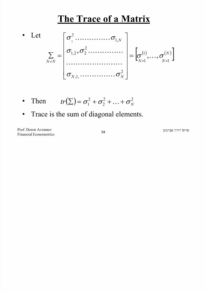
The Trace of a Matrix
• Let
• Then
• Trace is the sum of diagonal elements.
'Prof. Doron AvramovFinancial Econometrics
54
( ) ( )[ ]111
2
,1,
2
22,1
,1
2
,,,
1
××× =
=∑ N
N
N
N N
N
N N σ σ
σ σ
σ σ
σ σ
K
KKKKK
KKKKKKKK
KKKKK
KKKKK
( )
22
2
2
1 N tr σ σ σ +++=∑K
Matrix Vectorization
8/22/2019 Avramov Doron Financial Econometrics
http://slidepdf.com/reader/full/avramov-doron-financial-econometrics 55/553
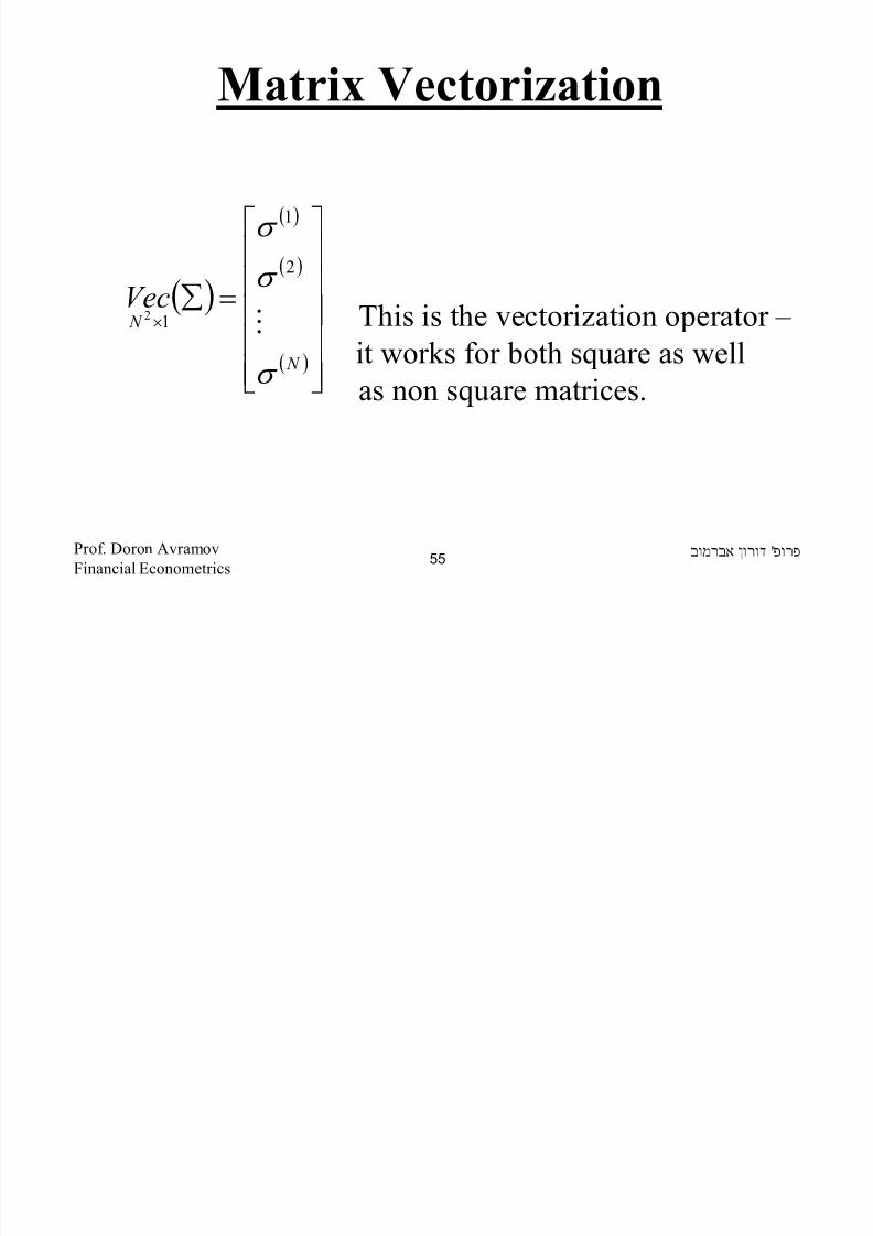
Matrix Vectorization
This is the vectorization operator –
it works for both square as well
as non square matrices.
'Prof. Doron AvramovFinancial Econometrics
55
( )
( )
( )
( )
=∑×
N
N Vec
σ
σ
σ
M
2
1
12
The VECH Operator

8/22/2019 Avramov Doron Financial Econometrics
http://slidepdf.com/reader/full/avramov-doron-financial-econometrics 56/553
The VECH Operator
•Similar to but takes only the distinct elements
of .
'Prof. Doron AvramovFinancial Econometrics
56
( )( )
( )
=∑×
+
2
2
2
2
1
1
12
1
N
N N N
Vech
σ
σ
σ
σ
M
M
( )∑Vec
∑
Partitioned Matrices

8/22/2019 Avramov Doron Financial Econometrics
http://slidepdf.com/reader/full/avramov-doron-financial-econometrics 57/553
•A, a square nonsingular matrix, is partitioned as
•Then the inverse of A is given by
•Check that
'Prof. Doron AvramovFinancial Econometrics
57
=
××
××
2212
2111
2221
1211
,
,
mmmm
mmmm
A A
A A
A
( ) ( )
( )
−−−
−−−=
−−−
−−−−
12
1
112122
1
2122121121
1
22
22
1
12
1
21221211
1
212212111
,
,
A A A A A A A A A A
A A A A A A A A A A A
( )21
1
mm I A A +− =⋅
Matrix Differentiation

8/22/2019 Avramov Doron Financial Econometrics
http://slidepdf.com/reader/full/avramov-doron-financial-econometrics 58/553
• Y is an M -vector. X is an N -vector. Then
• Let
'Prof. Doron AvramovFinancial Econometrics
58
∂∂
∂∂
∂∂
∂∂
∂∂
∂∂
=∂∂
×
N
M M M
N
N M
X
Y
X
Y
X
Y
X
Y
X
Y
X
Y
X
Y
,,,
,,,
21
1
2
1
1
1
K
M
K
A X
Y =
∂∂
11 ×××=
N N M M X AY
Matrix Differentiation

8/22/2019 Avramov Doron Financial Econometrics
http://slidepdf.com/reader/full/avramov-doron-financial-econometrics 59/553
Matrix Differentiation
• Let
'Prof. Doron AvramovFinancial Econometrics
59
''
'
A X Y
Z
AY X
Z
=∂∂
=∂∂
11'
×××=
N N M M X AY Z
Matrix Differentiation

8/22/2019 Avramov Doron Financial Econometrics
http://slidepdf.com/reader/full/avramov-doron-financial-econometrics 60/553
Matrix Differentiation
• Let
• If C is symmetric, then
'Prof. Doron AvramovFinancial Econometrics
60
( )'' C C X
X
+=
∂
∂θ
11'
×××=
N N N N X C X θ
C X X
'2=∂∂θ
Kronecker Product:

8/22/2019 Avramov Doron Financial Econometrics
http://slidepdf.com/reader/full/avramov-doron-financial-econometrics 61/553
•It is given by
g pmnmg np B AC ××× ⊗=
=×
Ba Ba
Ba BaC
nmn
m
mg np
,
,
1
111
KKKKK
KKKKKKKKK
KKKKK
'Prof. Doron AvramovFinancial Econometrics
61
Kronecker Product:
Kronecker Product:

8/22/2019 Avramov Doron Financial Econometrics
http://slidepdf.com/reader/full/avramov-doron-financial-econometrics 62/553
For A,B square matrices, it follows that
'Prof. Doron AvramovFinancial Econometrics62
( )
( )( ) ( ) BD AC DC B A
B A B A
B A B A N M
N N M M
⊗=⊗⊗
=⊗⊗=⊗
××
−−− 111
Operations on Matrices
8/22/2019 Avramov Doron Financial Econometrics
http://slidepdf.com/reader/full/avramov-doron-financial-econometrics 63/553
Operations on Matrices
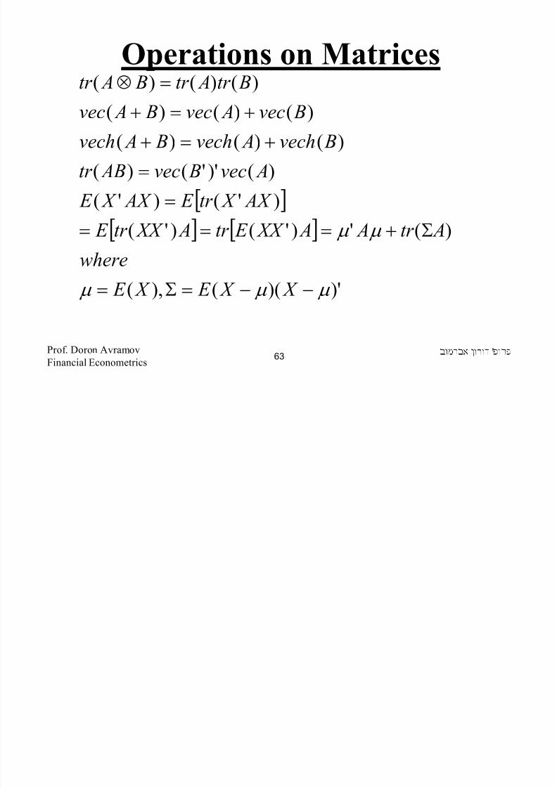
'Prof. Doron AvramovFinancial Econometrics63
[ ][ ] [ ]
)')((),(
)(')'()'(
)'()'(
)()''()()()()(
)()()(
)()()(
µ µ µ
µ µ
−−=Σ=
Σ+===
=
= +=+
+=+=⊗
X X E X E
where
Atr A A XX E tr A XX tr E
AX X tr E AX X E
Avec Bvec ABtr Bvech Avech B Avech
Bvec Avec B Avec
Btr Atr B Atr
Using Matrix Notation in a Portfolio

8/22/2019 Avramov Doron Financial Econometrics
http://slidepdf.com/reader/full/avramov-doron-financial-econometrics 64/553
The expectation and the variance of a portfolio’s rate of
return in the presence of three stocks are formulated as
ω ω
ρ σ σ ω ω ρ σ σ ω ω ρ σ σ ω ω
σ ω σ ω σ ω σ
µ ω µ ω µ ω µ ω µ
∑=
+++++=
=++=
'
222
'
233232133131122121
23
23
22
22
21
21
2
332211
p
p
'Prof. Doron AvramovFinancial Econometrics64
Choice Context
Using Matrix Notation in a Portfolio

8/22/2019 Avramov Doron Financial Econometrics
http://slidepdf.com/reader/full/avramov-doron-financial-econometrics 65/553
where
=×
3
2
1
13
ω
ω
ω
ω
=∑×
2
33231
23
2
221
1312
2
1
33
,,
,,
,,
σ σ σ
σ σ σ
σ σ σ
=×
3
2
1
13
µ
µ
µ
µ
'Prof. Doron AvramovFinancial Econometrics 65
Choice Context
The Expectation, Variance, and

8/22/2019 Avramov Doron Financial Econometrics
http://slidepdf.com/reader/full/avramov-doron-financial-econometrics 66/553
Covariance of Sum of RandomVariables
)()()()( z cE ybE xaE cz byax E ++=++
'Prof. Doron AvramovFinancial Econometrics 66
),(2),(2),(2
)()()()( 222
z ybcCov z xacCov y xabCov
z Var c yVar b xVar acz byaxVar
+++
++=++
),(),(),(),(),(
w ybdCov z ybcCovw xadCov z xacCovdwcz byaxCov
+++=++
Law of Iterated Expectations (LIE)

8/22/2019 Avramov Doron Financial Econometrics
http://slidepdf.com/reader/full/avramov-doron-financial-econometrics 67/553
Law of Iterated Expectations (LIE)
• The LIE relates the unconditional expectation of a
random variable to its conditional expectation via the
formulation
• Paul Samuelson shows the relation between the LIE andthe notion of market efficiency – which loosely speaking
asserts that the change in asset prices cannot be predicted
using current information.
Prof. Doron AvramovFinancial Econometrics
[ ] [ ] X Y E E Y E x |=
'67
LIE and Market Efficiency

8/22/2019 Avramov Doron Financial Econometrics
http://slidepdf.com/reader/full/avramov-doron-financial-econometrics 68/553
LIE and Market Efficiency
• Under rational expectations, the time t security
price can be written as the rational expectation of
some fundamental value, conditional on informationavailable at time t :
• Similarly,• The conditional expectation of the price change is
• The quantity does not depend on the information.
][| ** P E I P E P t t t ==
Prof. Doron AvramovFinancial Econometrics
][|
*
11
*
1 P E I P E P t t t +++ ==
0][][]|[**
11 =−=− ++ P E P E E I P P E t t t t t t
'68
Variance Decomposition (VD)

8/22/2019 Avramov Doron Financial Econometrics
http://slidepdf.com/reader/full/avramov-doron-financial-econometrics 69/553
Variance Decomposition (VD)
• Let us decompose :
• Shiller (1981) documents excess volatility in the
equity market. We can use VD to prove it:
• The theoretical stock price:
based on actual future dividends
• The actual stock price:
[ ] yVar
[ ] ( )[ ] ( )[ ] x yVar E x y E Var yVar x x || +=
t t t I P E P *=
( )LL
2
21*
11 r
D
r
D P t t
t +
++
= ++
'Prof. Doron AvramovFinancial Econometrics 69

8/22/2019 Avramov Doron Financial Econometrics
http://slidepdf.com/reader/full/avramov-doron-financial-econometrics 70/553
Variance Decomposition
What do we observe in the data? The opposite!!
t t t t t I P Var E I P E Var P Var *** +=
[ ] positive P Var P Var t t +=* positive
[ ]t t P Var P Var >*
'Prof. Doron AvramovFinancial Econometrics 70

8/22/2019 Avramov Doron Financial Econometrics
http://slidepdf.com/reader/full/avramov-doron-financial-econometrics 71/553
Lecture Notes in Financial
Econometrics
Taylor Approximations inFinancial Economics
'Prof. Doron Avramov
Financial Econometrics 71
TA in Finance

8/22/2019 Avramov Doron Financial Econometrics
http://slidepdf.com/reader/full/avramov-doron-financial-econometrics 72/553
• Several major applications in finance require the use of
Taylor series approximation.
• See three applications in the following table.
• We will also derive a test statistic for the Sharpe ratio –
the price of risk – which is based on the delta method,
which in turn is using the first order Taylor
approximation.
'Prof. Doron Avramov
Financial Econometrics 72
TA in Finance: Major

8/22/2019 Avramov Doron Financial Econometrics
http://slidepdf.com/reader/full/avramov-doron-financial-econometrics 73/553
Applications
'Prof. Doron Avramov
Financial Econometrics 73
Expected Utility Bond Pricing Option Pricing
First Oder Mean Duration Delta
Second Order Volatility Convexity Gamma
Third Order Skewness
Fourth Order Kurtosis
8/22/2019 Avramov Doron Financial Econometrics
http://slidepdf.com/reader/full/avramov-doron-financial-econometrics 74/553
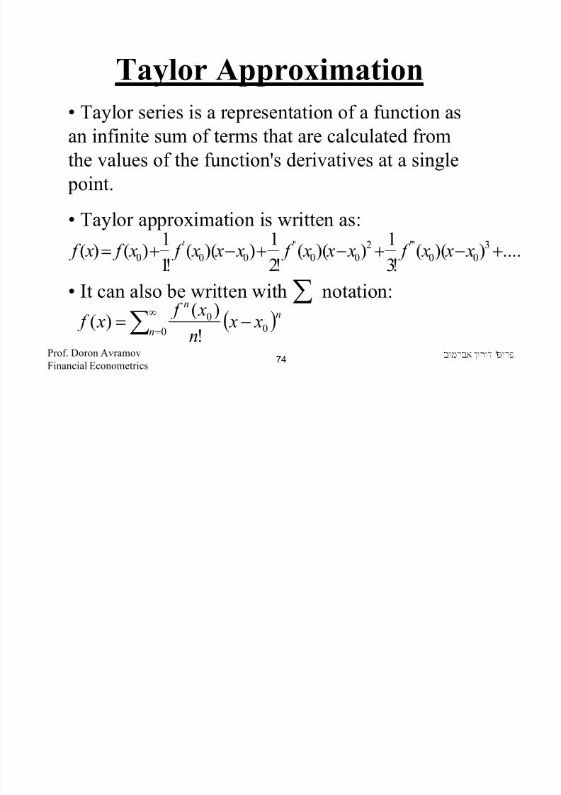
Taylor Approximation• Taylor series is a representation of a function as
an infinite sum of terms that are calculated from
the values of the function's derivatives at a single
point.
• Taylor approximation is written as:
• It can also be written with notation:
....))((!3
1))((
!2
1))((
!1
1)()( 3
00
'''2
00
''
00
'
0 +−+−+−+= x x x f x x x f x x x f x f x f
( )∑∞
=−=
0 00
!
)()(
n
nn
x xn
x f x f
∑
'Prof. Doron Avramov
Financial Econometrics 74
Maximizing Expected Utility of

8/22/2019 Avramov Doron Financial Econometrics
http://slidepdf.com/reader/full/avramov-doron-financial-econometrics 75/553
Terminal Wealth
).1)......(1)(1(1
)1(
21 K T T T
T K T
R R R Rwhere
RW W
+++
+
+++=+
+=
The invested wealth is
The investment horizon is K periods.
The terminal wealth, the wealth in the end of the investment
horizon, is
T W
'Prof. Doron Avramov
Financial Econometrics 75
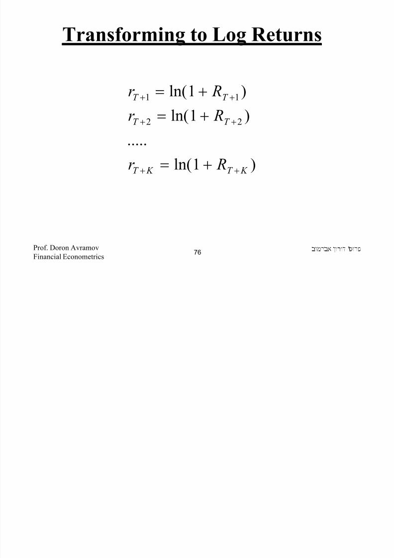
Transforming to Log Returns
8/22/2019 Avramov Doron Financial Econometrics
http://slidepdf.com/reader/full/avramov-doron-financial-econometrics 76/553
)1ln(
.....
)1ln(
)1ln(
22
11
K T K T
T T
T T
Rr
Rr
Rr
++
++
++
+=
+=
+=
'Prof. Doron Avramov
Financial Econometrics 76
Power utility as a Function of

8/22/2019 Avramov Doron Financial Econometrics
http://slidepdf.com/reader/full/avramov-doron-financial-econometrics 77/553
• Assume that the investor has the power utility function
of the from
• The cumulative log return (CLR) over the investment
horizon is:
• The terminal wealth as a function of CLR is
'Prof. Doron Avramov
Financial Econometrics 77
K T K T W W u ++ =γ
γ
1)(
K T T T r r r r +++ +++= ...21
)exp()1( r W RW W T T K T =+=+
Log Return
Power utility as a Function of

8/22/2019 Avramov Doron Financial Econometrics
http://slidepdf.com/reader/full/avramov-doron-financial-econometrics 78/553
• Then the utility function of terminal wealth can be
expressed as a function of CLR
• We can use the TA to express the utility as a function
of the moments of CLR.
• That is, we will approximate around
'Prof. Doron Avramov
Financial Econometrics 78
)exp(11
)( r W W W u T k T K T γ γ γ
γ γ == ++
)( K T W u + )(r E =µ
Log Return
The Utility Function

8/22/2019 Avramov Doron Financial Econometrics
http://slidepdf.com/reader/full/avramov-doron-financial-econometrics 79/553
'Prof. Doron Avramov
Financial Econometrics 79
])(24
1)(
6
1
)(2
11)[exp()]([
....))(exp(24
1
))(exp(6
1))(exp(
2
1
))(exp()exp()(
43
2
44
3322
γ γ
γ µγ γ
γ µ µγ
γ µ µγ γ µ µγ
γ µ µγ γ
µγ γ
γ
γ γ
r Kur r Ske
r Var W
W u E
r
r r
r W W
W u
T K T
T T K T
+
++≈
+−+
−+−+
−+=
+
+
Approximation
Expected Utility

8/22/2019 Avramov Doron Financial Econometrics
http://slidepdf.com/reader/full/avramov-doron-financial-econometrics 80/553
Let us assume that log return is normally distributed:
The exact solution under normality is
[ ]
++≈⋅
== →
4422
42
821)exp(:
3,0),(~
σ γ σ γ γµ γ
σ σ µ
γ T W E Then
Kur Ske N r
'Prof. Doron Avramov
Financial Econometrics 80
[ ]
+=⋅ 2
2
2
exp σ γ
γµ
γ
γ
T W E
Taylor Approximation – Bond Pricing

8/22/2019 Avramov Doron Financial Econometrics
http://slidepdf.com/reader/full/avramov-doron-financial-econometrics 81/553
• Taylor approximation is also used in bond pricing.
• The bond price is:
where y0 is the yield to maturity.
• Assume that y0 changes to y1
• The delta (the change) of the yield to maturity is written
as:
( )∑ =
+
=n
i i
i
y
CF y P
1
0
0
1
)(
01 y y y −=∆
'Prof. Doron Avramov
Financial Econometrics 81
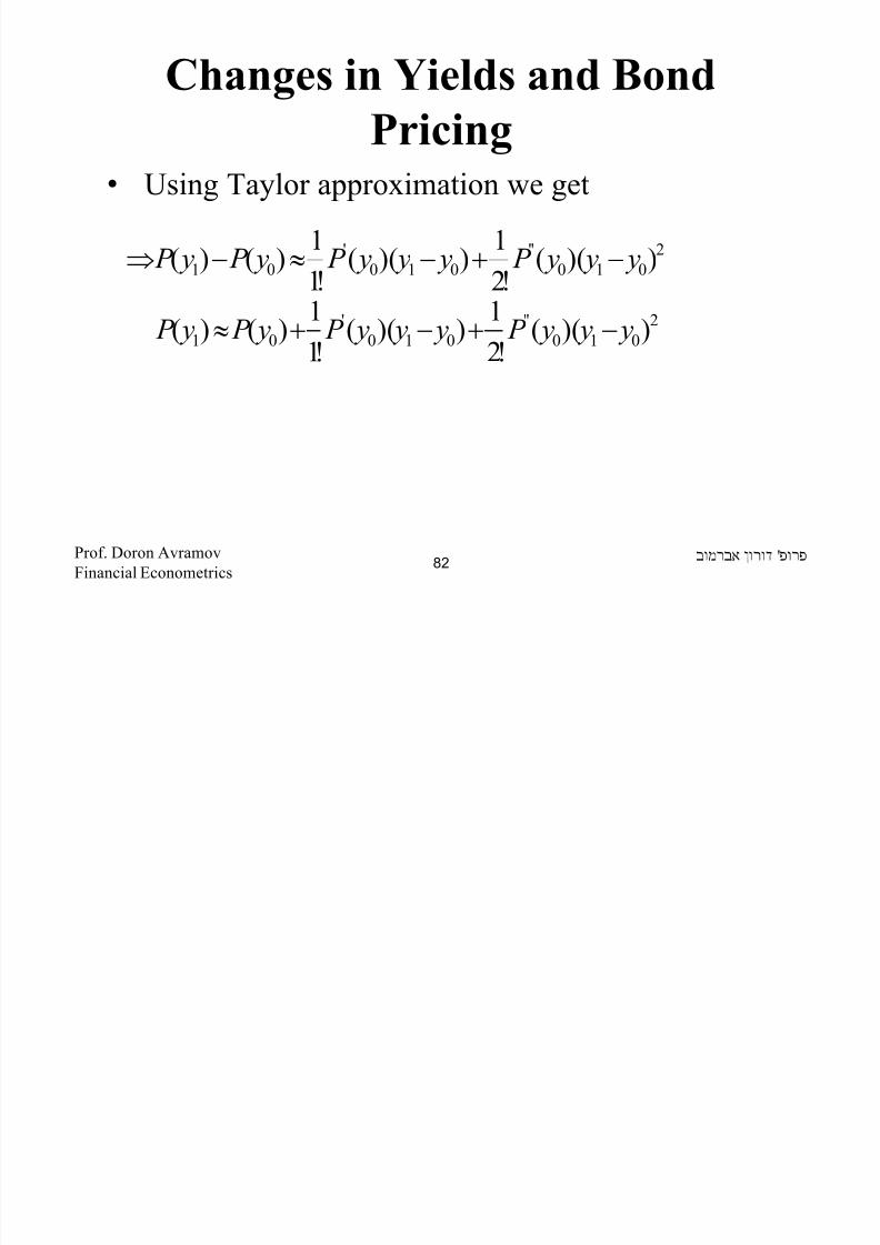
Changes in Yields and Bond
8/22/2019 Avramov Doron Financial Econometrics
http://slidepdf.com/reader/full/avramov-doron-financial-econometrics 82/553
Pricing• Using Taylor approximation we get
2
010
''
010
'
01
))((!2
1))((
!1
1)()( y y y P y y y P y P y P −+−+≈
2
010
''
010
'
01 ))((!2
1))((!11)()( y y y P y y y P y P y P −+−≈−⇒
'Prof. Doron Avramov
Financial Econometrics 82
Duration and Convexity

8/22/2019 Avramov Doron Financial Econometrics
http://slidepdf.com/reader/full/avramov-doron-financial-econometrics 83/553
• Dividing by P(y0 ) yields
•Instead of: we can write “-MD”
(Modified Duration).
•Instead of: we can write “Con”(Convexity).
)(2
)(
)(
)(
0
2
0
''
0
0
'
y P
y y P
y P
y y P
P
P ∆⋅+
∆⋅≈
∆
)(
)(
0
0
'
y P
y P
)()(
0
0
''
y P y P
'Prof. Doron Avramov
Financial Econometrics 83
The Approximated Bond Price

8/22/2019 Avramov Doron Financial Econometrics
http://slidepdf.com/reader/full/avramov-doron-financial-econometrics 84/553
Change• It is given by
• What if the yield to maturity falls?
2
2 yCon y MD
P
P ∆⋅+∆⋅−≈
∆
'Prof. Doron Avramov
Financial Econometrics 84
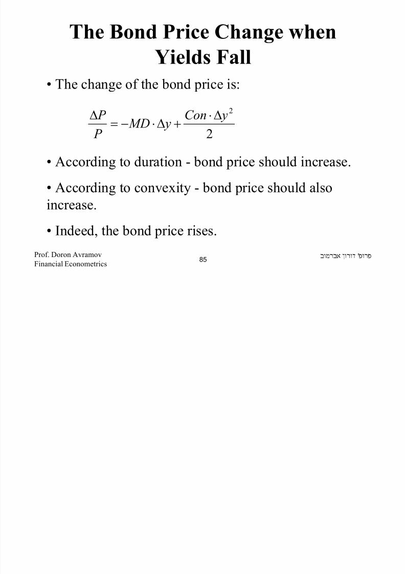
The Bond Price Change when
8/22/2019 Avramov Doron Financial Econometrics
http://slidepdf.com/reader/full/avramov-doron-financial-econometrics 85/553
• The change of the bond price is:
• According to duration - bond price should increase.
• According to convexity - bond price should also
increase.• Indeed, the bond price rises.
2
2 yCon y MD
P
P ∆⋅+∆⋅−=∆
'Prof. Doron Avramov
Financial Econometrics 85
Yields Fall
The Bond Price Change when

8/22/2019 Avramov Doron Financial Econometrics
http://slidepdf.com/reader/full/avramov-doron-financial-econometrics 86/553
• And what if the yield to maturity increases?
• Again, the change of the bond price is:
• According to duration – the bond price should
decrease.
2
2 yCon y MD
P
P ∆⋅+∆⋅−=
∆
'Prof. Doron Avramov
Financial Econometrics 86
Yields Increase
The Bond Price Change when
Yi ld I

8/22/2019 Avramov Doron Financial Econometrics
http://slidepdf.com/reader/full/avramov-doron-financial-econometrics 87/553
• According to convexity - bond price should increase.
• So what is the overall effect?
• Notice: the influence of duration is always stronger
than that of convexity as the duration is a first order effect while the convexity is second order.
'Prof. Doron Avramov
Financial Econometrics 87
Yields Increase
Option Pricing

8/22/2019 Avramov Doron Financial Econometrics
http://slidepdf.com/reader/full/avramov-doron-financial-econometrics 88/553
• A call price is a function of the underlying asset price
• What is the change in the call price when the
underlying asset pricing changes?
• Focusing on the first order term – this establishes the
delta neutral trading strategy.
( ) ( )
( ) ( )2
2
2
2
2
1)(
2
1
)()(
t st st
t st st s
P P P P P C
P P P
C
P P P
C
P C P C
−Γ+−∆+≈
−∂
∂
+−∂
∂
+≈
'Prof. Doron Avramov
Financial Econometrics 88
Delta Neutral Strategy

8/22/2019 Avramov Doron Financial Econometrics
http://slidepdf.com/reader/full/avramov-doron-financial-econometrics 89/553
Suppose that the underlying asset volatility increases.
Suppose further the implied volatility lags behind.
The call option is then underpriced – buy the call.
However, you take the risk of fluctuations in the price
of the underlying asset.
To hedge that risk you sell Delta units of theunderlying asset.
'Prof. Doron Avramov
Financial Econometrics 89

8/22/2019 Avramov Doron Financial Econometrics
http://slidepdf.com/reader/full/avramov-doron-financial-econometrics 90/553
Lecture Notes in Financial
Econometrics
OLS, MLE, MOM
'Prof. Doron Avramov
Financial Econometrics 90
Ordinary Least Squares (OLS)
h l i i h i

8/22/2019 Avramov Doron Financial Econometrics
http://slidepdf.com/reader/full/avramov-doron-financial-econometrics 91/553
• The goal is to estimate the regression parameters.
• Using optimization can help us reach the goal.
• Consider the regression:
, ,
∑=
=
−=
+=
T
T
t
t t t
t t t
f
x y
x y
1
2
)( ε
β ε
ε β
β
=
T y
y
Y .
1
=
KT T
K
x x
x x
X
,,,1
,,,1
1
111
K
KKKKK
K
=
T
E
ε
ε
.
1
'Prof. Doron Avramov
Financial Econometrics 91
• First Order Conditions
L t d i th f ti ith t t b t d

8/22/2019 Avramov Doron Financial Econometrics
http://slidepdf.com/reader/full/avramov-doron-financial-econometrics 92/553
• Let us derive the function with respect to beta and
make the derivative equal to zero
• Recall: X and Y are observations based on real data.
• Could we choose other to obtain smaller
Y X X X
Y X X X f
'1'
'')(
)(ˆ
02)(2
−=
=−=∂
∂
β
β β β
β ∑=
=T
T
t E E 1
2' ε
'Prof. Doron Avramov
Financial Econometrics 92
• o! Because the optimization minimizes the quantity
The OLS Estimator

8/22/2019 Avramov Doron Financial Econometrics
http://slidepdf.com/reader/full/avramov-doron-financial-econometrics 93/553
.
• We know:
• Is the estimator unbiased for ?
, So – it is indeed unbiased.
E X X X
E X X X X X X X E X X X X E X Y
'1'
'1''1'
'1'
)(ˆ
)()(ˆ)()(
ˆ
−
−−
−
+=
+=+=→+=
β β
β β β β β
β β
[ ][ ] 0)(
)(
ˆ
'1'
'1'
==
=
−
−
−
E E X X X
E X X X E
E β β
E '
'Prof. Doron Avramov
Financial Econometrics 93
• What about the Standard Error of ?β
The Standard Errors of the OLS Estimates

8/22/2019 Avramov Doron Financial Econometrics
http://slidepdf.com/reader/full/avramov-doron-financial-econometrics 94/553
• What about the Standard Error of ?
• Reminder:
β
( ) ( )
−⋅−=
'ˆˆ)ˆ( β β β β β E VAR
( ) 1'''
'1'
)(ˆ
)(ˆ
−
−
=−
=−
X X X E
E X X X
β β
β β
'Prof. Doron Avramov
Financial Econometrics 94
Continuing:
The Standard Errors of the OLS Estimates

8/22/2019 Avramov Doron Financial Econometrics
http://slidepdf.com/reader/full/avramov-doron-financial-econometrics 95/553
where K is the number of explanatory variables in
the regression specification.
[ ]
E E K T
X X X X X X X EE E X X X
X X X EE X X X E
ˆˆ1
1ˆ
ˆ)(ˆ
ˆ)()()(
)()(
'2
21'
21'1'''1'
1'''1'
−−=
=∑=
=
−
−−−
−−
ε
ε β
ε
σ
σ σ
'Prof. Doron Avramov
Financial Econometrics 95
MLE
• We next turn to resorting to Maximum Likelihood as a
8/22/2019 Avramov Doron Financial Econometrics
http://slidepdf.com/reader/full/avramov-doron-financial-econometrics 96/553
• We next turn to resorting to Maximum Likelihood as a
powerful tool for both estimating regression parameters
as well as testing models.
• The MLE is an asymptotic procedure and it a
parametric approach in that the distribution of the
regression residual must be specified explicitly.
'Prof. Doron Avramov
Financial Econometrics 96
Implementing MLE
A h ( )2N
iid

8/22/2019 Avramov Doron Financial Econometrics
http://slidepdf.com/reader/full/avramov-doron-financial-econometrics 97/553
• Assume that
• Let us estimate and using MLE; then derive
the joint distribution of these estimates.
• Under normality, the probability distribution
function ( pdf ) of the rate of return takes the form
( )2,~ σ µ N r t
µ 2σ
( )
−−=
2
2
2 2
1exp
2
1)(
σ
µ
πσ
t t
r r pdf
'Prof. Doron Avramov
Financial Econometrics 97
The Joint Likelihood
( ) ( ) ( ) ( )rpdfrrrpdfrrrpdfrrrpdfL ×××== 322121

8/22/2019 Avramov Doron Financial Econometrics
http://slidepdf.com/reader/full/avramov-doron-financial-econometrics 98/553
• Since stock returns are assumed iid - it follows that
• Now take the natural log of the joint likelihood:
( ) ( ) ( )
( )
−
−=
×××=
∑=
−T
T
t T
T
r L
r pdf r pdf r pdf L
1
2
22
21
2
1exp2
σ
µ πσ
K
( ) ( ) ∑=
−−−−=
T
t
t r T T L1
2
2
21ln
22ln
2ln
σ µ σ π
( ) ( ) ( ) ( )T T T T r pdf r r r pdf r r r pdf r r r pdf L ×××== KKKK 322121 ,,,
'Prof. Doron Avramov
Financial Econometrics 98
MLE: Sample Estimates
• Derive the first order conditions

8/22/2019 Avramov Doron Financial Econometrics
http://slidepdf.com/reader/full/avramov-doron-financial-econometrics 99/553
• Derive the first order conditions
Since - the variance estimator is not
unbiased.
( )( )∑ ∑
∑∑
= =
==
−=→=−
+−=
∂
∂
=→=
−
=∂
∂
T
t
T
t
t t
T
t t
T
t
t
r
T
r T L
r T
r L
1 1
22
4
2
22
112
ˆ1
ˆ0
2
ln
1
ˆ0
ln
µ σ
σ
µ
σ σ
µ σ
µ
µ
22ˆ σ σ ≠ E
'Prof. Doron Avramov
Financial Econometrics 99
MLE: The Information Matrix
• Take second derivatives:

8/22/2019 Avramov Doron Financial Econometrics
http://slidepdf.com/reader/full/avramov-doron-financial-econometrics 100/553
• Take second derivatives:
( )
( )
( )
∑
∑
∑
=
=
=
−=
∂
∂→
−−=
∂
∂
=
∂∂
∂→
−−=
∂∂
∂
−=
∂
∂
→−=−=∂
∂
T
t
t
T
t
t
T
t
T L E
r T L
L E
r L
T L
E
T L
1422
2
4
2
422
2
1
2
2
42
2
21
2
2
222
2
2
ln
2
ln
0lnln
ln1ln
σ σ
σ
µ
σ σ
σ µ σ
µ
σ µ
σ µ σ σ µ
'Prof. Doron Avramov
Financial Econometrics 100
MLE: The Covariance Matrix
• Set the information matrix ∂= ln)(2
θ LEI

8/22/2019 Avramov Doron Financial Econometrics
http://slidepdf.com/reader/full/avramov-doron-financial-econometrics 101/553
• Set the information matrix
• Then the asy. distribution of the parameters is
In our context, the information matrix is derived as
∂∂∂−=
'ln)(θ θ
θ L E I
→
→
−
−−
T
T
T
T
T
T INVERSE MULTIPLY
4
2
4
2"1"
4
2
2,0
0,
2,0
0,
2,0
0,
σ
σ
σ
σ
σ
σ
( )1)(,0~
−∧
− θ θ θ I N T
'Prof. Doron Avramov
Financial Econometrics 101
To Summarize
•The asy distribution of the parameters is

8/22/2019 Avramov Doron Financial Econometrics
http://slidepdf.com/reader/full/avramov-doron-financial-econometrics 102/553
The asy. distribution of the parameters is
In our context, the joint distribution of the sample
mean and variance assuming IID normal is
( )1)(,0~
−∧
− θ θ θ I N T
−−
−
∑∑
∑
==
=
4
2
2
11
2
1
2,0
0,,
0
0~
)1(1
1
σ
σ
σ
µ
N
r T
r T
r T
T T
t
t
T
t
t
T
t
t
'Prof. Doron Avramov
Financial Econometrics 102
The Sample Mean and Variance
• Notice that when returns are normally distributed –

8/22/2019 Avramov Doron Financial Econometrics
http://slidepdf.com/reader/full/avramov-doron-financial-econometrics 103/553
Notice that when returns are normally distributed
the sample mean and variance are independent.
• That would not be the case otherwise.
• Departing from normality, the covariance between the
sample mean and variance is the skewness (see below).• Notice also that the ratio obtained by dividing the
variance of the variance by the variance of the mean is
smaller than one as long as volatility is below 70%.
• Clearly, the mean return estimate is more noisy.'Prof. Doron Avramov
Financial Econometrics 103
Departing from Normality:
Setting Moment Conditions

8/22/2019 Avramov Doron Financial Econometrics
http://slidepdf.com/reader/full/avramov-doron-financial-econometrics 104/553
Setting Moment Conditions• We know:
• If:
•Then:
• That is, we set two momentum conditions.
( )
( )22
σ µ
µ
=−
=
t
t
r E
r E
( )( )
−−
−=
22σ µ
µ θ
t
t
t r
r g
( )
=
0
0t g E
'Prof. Doron Avramov
Financial Econometrics 104
Method of Moments (MOM)
• There are two parameters: 2σµ

8/22/2019 Avramov Doron Financial Econometrics
http://slidepdf.com/reader/full/avramov-doron-financial-econometrics 105/553
There are two parameters:
• Stage 1: Moment Conditions
• Stage 2: estimation
,σ µ
( )
−−−=
22σ µ
µ
t
t
t r
r g
01
1
^
=∑=
T
t
t g T
'Prof. Doron Avramov
Financial Econometrics 105
Method of Moments
• Continue estimation:

8/22/2019 Avramov Doron Financial Econometrics
http://slidepdf.com/reader/full/avramov-doron-financial-econometrics 106/553
Continue estimation:
( )
( )[ ]
( )∑
∑
∑
∑
=
=
=
−=
=−−
=
=−
T
t
t
T
t
t
T
t
t
t
r
T
r T
r T
r
T
1
22
1
22
1
ˆ1
ˆ
0ˆˆ1
1ˆ
0ˆ1
µ σ
σ µ
µ
µ
'Prof. Doron Avramov
Financial Econometrics106
T t ,,1 K=
MOM: Stage 3

8/22/2019 Avramov Doron Financial Econometrics
http://slidepdf.com/reader/full/avramov-doron-financial-econometrics 107/553
)'
t t g g E S =
− 4
43
3
2
,
,
σ µ µ
µ σ
( ) ( ) ( )( ) ( ) ( ) ( )
+−−−−−−
−−−−=
422423
232
2,
,
σ µ σ µ µ σ µ
µ σ µ µ
t t t t
t t t
r r r r
r r r E S
'Prof. Doron Avramov
Financial Econometrics107
MOM: stage 4
M

8/22/2019 Avramov Doron Financial Econometrics
http://slidepdf.com/reader/full/avramov-doron-financial-econometrics 108/553
• Memo:
• Stage 4: derive wrt and take the expected
value
( )( )
−−
−=
22σ µ
µ θ
t
t
t r
r g
( )θ t g θ
( )( )
−
−=
−−−
−=
∂∂=
1,0
0,1
1,2
0,1
µ θ
θ
t
t
r E
g E D
'Prof. Doron Avramov
Financial Econometrics108
MOM: The Covariance Matrix
Stage 5:

8/22/2019 Avramov Doron Financial Econometrics
http://slidepdf.com/reader/full/avramov-doron-financial-econometrics 109/553
g
( )S
DS D
=∑
=∑−−
θ
θ
11'
'Prof. Doron Avramov
Financial Econometrics109
The Covariance Matrices
=∑21 0,σ
θ =∑ 322 ,µ σ θ

8/22/2019 Avramov Doron Financial Econometrics
http://slidepdf.com/reader/full/avramov-doron-financial-econometrics 110/553
∑42,0 σ
θ
−
∑4
43, σ µ µ θ
• Sample estimates of the Skewness and Kurtosis are
3
3 σ µ ×== sk SK
( )∑=
−=T
t
t r r T 1
3
3
1µ ( )∑
=
−=T
t
t r r T 1
4
4
1µ
sk is the skewness of the standardized
return
kr is the kurtosis of the standardizedreturn
4
4 σ µ ×== kr KR
110
Under Normality the MOM Covariance
Matrix Boils Down to

8/22/2019 Avramov Doron Financial Econometrics
http://slidepdf.com/reader/full/avramov-doron-financial-econometrics 111/553
1
44
43
32
2
2,0
0,θ θ
σ σ µ µ
µ σ Σ=
=−===∑
'Prof. Doron Avramov
Financial Econometrics111
MOM: Estimating Regression Parameters
• Let us run the time series regression

8/22/2019 Avramov Doron Financial Econometrics
http://slidepdf.com/reader/full/avramov-doron-financial-econometrics 112/553
• There are two moment conditions:
t mt t r r ε α +⋅+=
( )
( ) 0
0
=
=
t mt
t
r E
E
ε
ε
( )( )[ ]
[ ][ ]',',1
'
β α θ
θ
β α
β α
==
−=
⋅−−
⋅−−=
mt t
t t t
mt mt t
mt t
t
r x
xr x
r r r
r r g
'Prof. Doron Avramov
Financial Econometrics112
MOM: Estimating Regression Parameters
• Estimation:

8/22/2019 Avramov Doron Financial Econometrics
http://slidepdf.com/reader/full/avramov-doron-financial-econometrics 113/553
( )
=
=
=
=−
×
−
=
−
=
==
∑∑∑∑
mT
m
T
T
t
t t
T
t
t t
T
t
t t
T
t
t t
r
r
X
R X X X r x x x
x xT
r xT
,1
,1
011
1
2
'1'
1
1
1
'^
1
^'
1
KK
θ
θ
=
T r
r
R K
1
'Prof. Doron Avramov
Financial Econometrics113
MOM: Estimating Standard Errors
• Estimation of the covariance matrix

8/22/2019 Avramov Doron Financial Econometrics
http://slidepdf.com/reader/full/avramov-doron-financial-econometrics 114/553
T
X X
x xT
g
T D
x xT g g T S
t
T
t t
T
t
t
T
t t
T
t
t t
T
t
t T
'
)'(
1)(1
ˆ)'(
1
)'()(
1
11^
^
2
1
^
1
^
−=−=∂
∂
=
==
∑∑
∑∑
==
==
θ
θ
ε θ θ
'Prof. Doron Avramov
Financial Econometrics114
MOM: Estimating Standard Errors
• The covariance matrix estimate is thus

8/22/2019 Avramov Doron Financial Econometrics
http://slidepdf.com/reader/full/avramov-doron-financial-econometrics 115/553
•Then, asymptotically we get
1
1
21
11
)'(ˆ)'()'(
)'(
−
=
−
−−
=Σ
=Σ
∑ X X x x X X T
DS DT
t
t t t
T T T
ε θ
θ
'Prof. Doron Avramov
Financial Econometrics115
),0(~)(^
θ θ θ Σ− N T
Lecture Notes in Financial

8/22/2019 Avramov Doron Financial Econometrics
http://slidepdf.com/reader/full/avramov-doron-financial-econometrics 116/553
Lecture Notes in Financial
Econometrics
Hypothesis Testing
'Prof. Doron Avramov
Financial Econometrics116
Overview
A short brief of the major contents for today’s class:

8/22/2019 Avramov Doron Financial Econometrics
http://slidepdf.com/reader/full/avramov-doron-financial-econometrics 117/553
• Hypothesis testing
• TESTS: Skewness, Kurtosis, Bera-Jarque
• A first step to testing asset pricing models
• Deriving test statistic for the Sharpe ratio
'Prof. Doron Avramov
Financial Econometrics117
Hypothesis Testing
• Let us assume that a mutual fund invests in value
t k ( t k ith hi h ti f b k t k t)

8/22/2019 Avramov Doron Financial Econometrics
http://slidepdf.com/reader/full/avramov-doron-financial-econometrics 118/553
stocks (e.g., stocks with high ratios of book-to-market).
• Performance evaluation is mostly about running theregression of excess fund returns on the market premium
• The hypothesis testing for examining performance is
H0
: means no performanceH1: Otherwise
it
e
mt ii
e
it R R ε β α ++=
=iα
'Prof. Doron Avramov
Financial Econometrics118
Hypothesis Testing
• Errors emerge if we reject H 0 while it is true, or whend t j t H h it i

8/22/2019 Avramov Doron Financial Econometrics
http://slidepdf.com/reader/full/avramov-doron-financial-econometrics 119/553
we do not reject H 0 when it is wrong:
Reject H0Don’t
reject H0
Type 1
error
Good
decisionH0
Good
decision
Type 2 error H1
α True state
of world
'Prof. Doron Avramov
Financial Econometrics119
Hypothesis Testing - Errors
• is the first type error (size), while is the secondtype error (related to power)
α β

8/22/2019 Avramov Doron Financial Econometrics
http://slidepdf.com/reader/full/avramov-doron-financial-econometrics 120/553
type error (related to power).
• The power of the test is equal to 1- .
• We would prefer both and to be as small as
possible, but there is always a trade-off.
• When decreases increases and vice versa.
•The implementation of hypothesis testing requires the
knowledge of distribution theory.
β
α
α β
'Prof. Doron Avramov
Financial Econometrics120
Skewness, Kurtosis & Bera
Jarque Test Statistics

8/22/2019 Avramov Doron Financial Econometrics
http://slidepdf.com/reader/full/avramov-doron-financial-econometrics 121/553
q
• We aim to test normality of stock returns.
• We use three distinct tests to examine normality.
'Prof. Doron Avramov
Financial Econometrics121
• TEST 1 - Skewness (third moment)
Test I – Skewness

8/22/2019 Avramov Doron Financial Econometrics
http://slidepdf.com/reader/full/avramov-doron-financial-econometrics 122/553
• The setup for testing normality of stock return:
H0:
H1: otherwise
• Sample Skewness is
( 2,~ σ µ N Rt
∑=
−=
T
t
H t
T N
R
T S
1
36
,0~ˆ
ˆ1 0
σ
µ
'Prof. Doron Avramov
Financial Econometrics
122
• Multiplying S by we get ( )10~ NST T
Test I – Skewness

8/22/2019 Avramov Doron Financial Econometrics
http://slidepdf.com/reader/full/avramov-doron-financial-econometrics 123/553
• Multiplying S by , we get
• If the statistic value is higher (absolute value) than thecritical value e.g., the statistic is equal to -2.31, then
reject H 0, otherwise do not reject the null of nomrality.
( )1,0~6
N S 6
'Prof. Doron Avramov
Financial Econometrics
123
TEST 2 - Kurtosis

8/22/2019 Avramov Doron Financial Econometrics
http://slidepdf.com/reader/full/avramov-doron-financial-econometrics 124/553
• Kurtosis estimate is:
• After transformation:
∑=
−=
T
t
H t
T N R
T K 1
424
,3~ˆ
ˆ1 0
σ
µ
( ) ( )1,0~324
0
N K T
H
−
'Prof. Doron Avramov
Financial Econometrics
124
• The statistic is: ( ) ( )2~3 222 χ−+= KT
ST
BJ
TEST 3 - Bera-Jarqua Test

8/22/2019 Avramov Doron Financial Econometrics
http://slidepdf.com/reader/full/avramov-doron-financial-econometrics 125/553
The statistic is:
• Why ?
( ) ( )23246
χ + K S BJ
)2(2 χ
'Prof. Doron Avramov
Financial Econometrics
125
• If X1~N(0,1) , X2~N (0,1) & then:21 XX ⊥
TEST 3 - Bera-Jarqua Test

8/22/2019 Avramov Doron Financial Econometrics
http://slidepdf.com/reader/full/avramov-doron-financial-econometrics 126/553
If X 1 N(0,1) , X 2 N (0,1) & then:
• and are both standard normal and
they are independent random varaibles.
( )2~22
2
2
1 χ X X +
21 X X ⊥
S T 6 ( )324 − K
T
'Prof. Doron Avramov
Financial Econometrics
126
Chi Squared Test
• In financial economics, the Chi square test is
implemented quite frequently in hypothesis testing

8/22/2019 Avramov Doron Financial Econometrics
http://slidepdf.com/reader/full/avramov-doron-financial-econometrics 127/553
implemented quite frequently in hypothesis testing.
• Let us derive it.
• Suppose that:
Then:
( ) ( )
( ) ( ) ( ) N R R y y
I N R y
21''
2
1
~
,0~
χ µ µ
µ
−∑−=
−∑=−
−
'Prof. Doron Avramov
Financial Econometrics
127
Testing the CAPM
• For one the chi squared is used to test the CAPM

8/22/2019 Avramov Doron Financial Econometrics
http://slidepdf.com/reader/full/avramov-doron-financial-econometrics 128/553
• For one, the chi squared is used to test the CAPM
• There are a few tests based on time series and crosssection specifications. Let us start with the time series.
• The CAPM says that:• Thus, we first run the time-series market regressions:
)()(
e
mi
e
i R E R E β =
N
e
m N N
e
N
e
m
e
R R
R R
ε β α
ε β α
++=
++=
KKKKKKKK
1111
'Prof. Doron Avramov
Financial Econometrics
128
• The expected excess return for asset i is given by:
)()( emii
ei R E R E β α +=
Testing the CAPM

8/22/2019 Avramov Doron Financial Econometrics
http://slidepdf.com/reader/full/avramov-doron-financial-econometrics 129/553
• According to the CAPM, the intercept i is restricted
to be zero for every test asset.
• So, the joint hypothesis test is:
• While doing the estimation, we will never get .
• Rather, we examine whether the estimate is equal to
zero statistically. For example, the sample estimate could be -- nevertheless this estimate could be
insignificant, or it is statistically equal to zero.
)(α
otherwise H
H N
:
0:
1
210 === α α α K
005.0ˆ =α
'Prof. Doron Avramov
Financial Econometrics
129
0ˆ =α
The Test Statistic
• Estimate :
=α
α .ˆ
ˆ1
α

8/22/2019 Avramov Doron Financial Econometrics
http://slidepdf.com/reader/full/avramov-doron-financial-econometrics 130/553
• If:
and
• We get:
• Later we will develop the exact analytics of this test.
N α ˆ
( ) ( )
( )α
α
α
α α µ
∑
∑→∑
,0~ˆ
,~ˆ,~
0
N
N N R
H
( ) N
H 21'
0
~ˆˆ χ α α α
−
∑
'Prof. Doron Avramov
Financial Econometrics
130
Joint Hypothesis Test
• Y th ti i i
8/22/2019 Avramov Doron Financial Econometrics
http://slidepdf.com/reader/full/avramov-doron-financial-econometrics 131/553
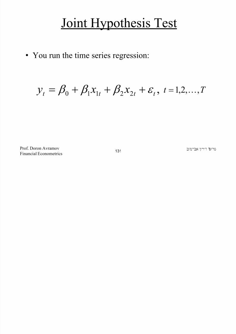
• You run the time series regression:
,22110 t t t t
x x y ε β β β +++= T t ,,2,1 K=
'Prof. Doron Avramov
Financial Econometrics
131
Joint Hypothesis Test
• We have three orthogonal conditions:( ) 0=t E ε

8/22/2019 Avramov Doron Financial Econometrics
http://slidepdf.com/reader/full/avramov-doron-financial-econometrics 132/553
• We have three orthogonal conditions:
• Using matrix notation:
( )
( ) 0
0
2
1
=
=
t t
t t
x E
x E
ε
ε
=×
T
T
y
y
Y ..
1
1
=×
T T
T
x x
x x
x x
X
21
2212
2111
3
,,1
,,1
,,1
KKKK[ ]'32113 ,, β β β β = x
11331 ×××× += T T T E X Y
=×
T
T E
ε
ε
.
.
1
1
'Prof. Doron Avramov
Financial Econometrics
132
• Let us assume that: , are iid (2
,0~ ε σ ε N t T ε ε ε ε K
321 ,,
Joint Hypothesis Test

8/22/2019 Avramov Doron Financial Econometrics
http://slidepdf.com/reader/full/avramov-doron-financial-econometrics 133/553
• Joint hypothesis testing:
( )( ) Y X X X
X X N '1'
21'
ˆ
,~ˆ−
−
= β
σ β β ε
otherwise H
H
:
0,1:
1
200 == β β
'Prof. Doron Avramov
Financial Econometrics
133
• Define: ,
= 1,0,0
0,0,1 R
= 0
1
q
Joint Hypothesis Test

8/22/2019 Avramov Doron Financial Econometrics
http://slidepdf.com/reader/full/avramov-doron-financial-econometrics 134/553
• The joint test becomes:
otherwise H
q R H
H
:
0
1
1,0,0
0,0,1
:
1
2
0
2
1
0
0
0
=
=
×
=
β
β
β
β β
β
'Prof. Doron Avramov
Financial Econometrics
134
q
• Returning to the testing:
otherwise H
q R H
:
0:
1
0 =− β
Joint Hypothesis Test

8/22/2019 Avramov Doron Financial Econometrics
http://slidepdf.com/reader/full/avramov-doron-financial-econometrics 135/553
• Under H0:
• Chi squared:
test statistic
( )',~ˆ R Rq R N q R
β β β ∑−−
( )',0~ˆ0
R R N q R H
β β ∑−
( ) ( ) ( ) ( )2~ˆˆ 21''
χ β β β q R R Rq R −∑−−
'Prof. Doron Avramov
Financial Econometrics
135
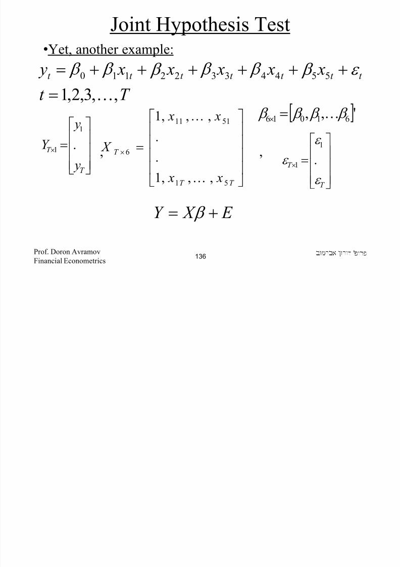
•Yet, another example:
t t t t t t t x x x x x y ε β β ++++++= 55443322110
Tt 321=
Joint Hypothesis Test
8/22/2019 Avramov Doron Financial Econometrics
http://slidepdf.com/reader/full/avramov-doron-financial-econometrics 136/553
, ,
=×
T
T
y
y
Y .
1
1
=×
T T
T
x x
x x
X
51
5111
6
,,,1
.
.
,,,1
K
K [ ]',, 61016 β β β β K=×
=×
T
T
ε
ε
ε .
1
1
T t ,,3,2,1 K=
E X Y += β
'Prof. Doron Avramov
Financial Econometrics
136
• Joint hypothesis test:
H 7,4
1,
3
1,
2
1,1: 532100 ===== β β β β β
Joint Hypothesis Test

8/22/2019 Avramov Doron Financial Econometrics
http://slidepdf.com/reader/full/avramov-doron-financial-econometrics 137/553
• Here is a receipt:1.
2.
3.
4.
otherwise H :
432
1
( )
( )( ) β ε
ε
σ β β
σ
β
β
∑=
⋅
−
=
−=
=
−
−
21'
'2
'1'
,~ˆ
ˆˆ
6
1ˆ
ˆˆ
ˆ
X X N
E E
T
X Y E
Y X X X
'Prof. Doron Avramov
Financial Econometrics
137
5.
=
=1
2
1
1
000100
0,0,0,0,1,00,0,0,0,0,1
qR
Joint Hypothesis Test

8/22/2019 Avramov Doron Financial Econometrics
http://slidepdf.com/reader/full/avramov-doron-financial-econometrics 138/553
5.
6.
7.
8.
9.
=
=
7
4
1
3,
1,0,0,0,0,00,0,1,0,0,0
0,0,0,1,0,0 q R
( )( )
( )( ) ( ) ( )5~ˆˆ
,0~ˆ
,~ˆ
0:
21''
'
'
0
0
0
χ β β
β
β β
β
β
β
H
H
q R R Rq R
R R N q R
R Rq R N q R
q R H
−∑−
∑−
∑−−
=−
−
'Prof. Doron Avramov
Financial Econometrics
138
•There are five degrees of freedom implied by the five
restrictions on53210 ,,,, β β β β β
Joint Hypothesis Test

8/22/2019 Avramov Doron Financial Econometrics
http://slidepdf.com/reader/full/avramov-doron-financial-econometrics 139/553
• The chi-squared distribution is always positive.
53210 ,,,, βββββ
'Prof. Doron Avramov
Financial Econometrics
139
Shrinkage Methods
• One of the problems with the tests we have just

8/22/2019 Avramov Doron Financial Econometrics
http://slidepdf.com/reader/full/avramov-doron-financial-econometrics 140/553
displayed is that the decision is binary: Reject or donot reject (Classical econometrics) the null.
• The possibility of partly rejecting/accepting the null,
for example, does not exist.
'Prof. Doron Avramov
Financial Econometrics
140
Shrinkage Methods and the CAPM
• One can advocate a Bayesian approach in which
the proposed model (CAPM) is recognized to be non

8/22/2019 Avramov Doron Financial Econometrics
http://slidepdf.com/reader/full/avramov-doron-financial-econometrics 141/553
the proposed model (CAPM) is recognized to be non-
perfect, but at the same time it is worth something.
• For example, let us assign a 50% weight to theCAPM and 50% to data.
'Prof. Doron Avramov
Financial Econometrics
141
Shrinkage Methods and the CAPM
• 50% CAPM :
• 50% Data:
)()( emiei R E R E β =
) )e
m
ee
m
e R E R E R R 1111111 β α ε β α +=→++=

8/22/2019 Avramov Doron Financial Econometrics
http://slidepdf.com/reader/full/avramov-doron-financial-econometrics 142/553
• Data based estimate is the sample mean. (Check it!)
• Let us consider three Mutual funds, with each of the
fund managers has one of the following beliefs:
• M 1 – The CAPM is true
• M 2 – The CAPM is wrong
• M 3 - Mix (equally weights) between CAPM and the Data
) )mm 1111111 ββ
0=→α
0≠→ α
'Prof. Doron Avramov
Financial Econometrics
142
Shrinkage and Performance
• Over the last several decades, the third Mutual fundwould have had the best performance.

8/22/2019 Avramov Doron Financial Econometrics
http://slidepdf.com/reader/full/avramov-doron-financial-econometrics 143/553
• Using the mixing method improves the estimation of expected return.
• The Black Litterman method (coming up later) is also
a type of a shrinkage approach - it is more rigorous than
the one presented here.
• The weights are on the model versus views onexpected returns, either absolute or relative.
'Prof. Doron Avramov
Financial Econometrics
143
Estimating the Sample Sharpe Ratio
• You observe time series of returns on a stock, or a bond, or any investment vehicle (e.g., a mutual fund or
h d f d) (

8/22/2019 Avramov Doron Financial Econometrics
http://slidepdf.com/reader/full/avramov-doron-financial-econometrics 144/553
a hedge fund):
• You attempt to estimate the mean and the variance of
those returns, derive their distribution, and test whether
the Sharpe Ratio of that investment is equal to zero.
• Let us denote the set of parameters by
• The Sharpe ratio is equal to σ
µ θ
f r SR
−=)(
]',[ 2σ µ θ =
( T r r r ,,, 21 K
'Prof. Doron Avramov
Financial Econometrics144
MLE vs. MOM
• To develop a test statistic for the SR, we canimplement the MLE or MOM, depending upon our
ti b t th t di t ib ti

8/22/2019 Avramov Doron Financial Econometrics
http://slidepdf.com/reader/full/avramov-doron-financial-econometrics 145/553
assumption about the return distribution.
•Let us denote the sample estimates by
MLE MOM
( )2,~ σ µ N r iid
t
( ) ( )1,0~ˆθ θ θ ∑− N T
a
( ) ( )2,0~ˆθ θ θ ∑− N T
a
∧
θ
returns depart from
iid normal
'Prof. Doron Avramov
Financial Econometrics145
MLE vs. MOM
• As shown earlier, the asymptotic distribution usingeither MLE or MOM is normal with a zero mean but
distinct variance covariance matrices

8/22/2019 Avramov Doron Financial Econometrics
http://slidepdf.com/reader/full/avramov-doron-financial-econometrics 146/553
distinct variance covariance matrices.
( ) ( )1,0~ˆθ θ θ ∑− N T
MLE ( ) ( )2,0~ˆθ θ θ ∑− N T
MOM
'Prof. Doron Avramov
Financial Econometrics146
Distribution of the SR Estimate:The Delta Method
• We will show that ( ) ( )2,0~ˆSR
a
N SR RS T σ −

8/22/2019 Avramov Doron Financial Econometrics
http://slidepdf.com/reader/full/avramov-doron-financial-econometrics 147/553
• We use the Delta method to derive
• The delta method is based upon the first order Taylor
approximation.
2
SRσ
'Prof. Doron Avramov
Financial Econometrics147
Distribution of the SR Estimate:The Delta Method
• The first-order TA is∂SR
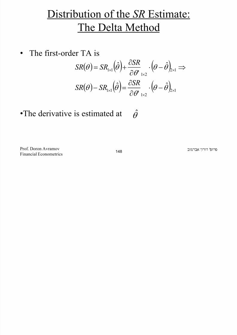
8/22/2019 Avramov Doron Financial Econometrics
http://slidepdf.com/reader/full/avramov-doron-financial-econometrics 148/553
•The derivative is estimated at
( ) ( ) ( )( ) ( ) ( ) 12
2111
1221
11
ˆ'
ˆ
ˆ'
ˆ
××
×
××
×
−⋅∂∂
=−
⇒−⋅∂
∂
+=
θ θ θ
θ θ
θ θ θ θ θ
SRSRSR
SR
SRSR
θ
'Prof. Doron Avramov
Financial Econometrics148
Distribution of the Sample SR
( ) ( )[ ] ( )( )'
0ˆˆ θ θ θ
θ θ E SR
E SRSR E =
−
∂∂
=−

8/22/2019 Avramov Doron Financial Econometrics
http://slidepdf.com/reader/full/avramov-doron-financial-econometrics 149/553
'Prof. Doron Avramov
Financial Econometrics149
( ) ( )( )
( ) ( )[ ] ( ) ( )[ ]
2
'
ˆˆ
ˆˆˆ
θ θ θ θ
θ θ θ θ θ
θ
SRSR E SRSRVAR
E VAR
MOREOVER
−=−
−−=
∂
The Variance of the SR
• Continue: ( )( )θ
θ θ θ θ θ
=
∂∂−−
∂∂ SRSR E
'
'ˆˆ

8/22/2019 Avramov Doron Financial Econometrics
http://slidepdf.com/reader/full/avramov-doron-financial-econometrics 150/553
( )( )
θ θ
θ θ θ θ θ
θ
θ ∂∂∑
∂∂=
=∂∂
−−
∂∂=
SRSR
SR E SR
'
'
'ˆˆ
'Prof. Doron Avramov
Financial Econometrics150
First Derivatives of the SR
• The SR is formulated as
•Let us derive:( ) 5.02σ
µ f
r SR
−=

8/22/2019 Avramov Doron Financial Econometrics
http://slidepdf.com/reader/full/avramov-doron-financial-econometrics 151/553
( ) ( ) ( )32
5.02
2 22
1
1
σ
µ
σ
µ σ
σ
σ µ
f f r r
SR
SR
−−=
−−
=∂∂
=
∂
∂
−
'Prof. Doron Avramov
Financial Econometrics151
The Distribution of SR under MLE
• Continue:
−∂∂ 2' 01 rSRSR σµ
1

8/22/2019 Avramov Doron Financial Econometrics
http://slidepdf.com/reader/full/avramov-doron-financial-econometrics 152/553
,
( ) +−⇒
−=∂
∂∑∂
∂
2
43
1
'
ˆ211,0~ˆ
2,0
0,
2,1
RS N RS SRT
r SRSR f
σ
σ
σ
µ
σ θ θ θ
−−
32σ
µ
σ
f r
'Prof. Doron Avramov
Financial Econometrics152
The Delta Method in General
• Here is the general application of the delta method
• If: ( )θ θ θ ∑− ,0~ˆ N T

8/22/2019 Avramov Doron Financial Econometrics
http://slidepdf.com/reader/full/avramov-doron-financial-econometrics 153/553
• Then let be some function of :
• where is the vector of derivatives of
with respect to
( )
( )θ d θ
( ) ( ) ( )'
,0~ˆ
θ θ θ θ θ D D N d d T ×∑×−( )θ D ( )θ d
θ
'Prof. Doron Avramov
Financial Econometrics153
Hypothesis Testing
• Does the S&P index outperform the Rf ?

8/22/2019 Avramov Doron Financial Econometrics
http://slidepdf.com/reader/full/avramov-doron-financial-econometrics 154/553
H 0: SR=0
H 1: Otherwise
• Under the null there is no outperformance.
• Thus, under the null
)1,0(~ˆ1
ˆ
)ˆ1,0(~ˆ
2
2
N RS
RS T
RS N RS T
+
+
'Prof. Doron Avramov
Financial Econometrics154
Lecture Notes in
Financial Econometrics

8/22/2019 Avramov Doron Financial Econometrics
http://slidepdf.com/reader/full/avramov-doron-financial-econometrics 155/553
The Efficient Frontier and theTangency Portfolio
'Prof. Doron Avramov
Financial Econometrics155
Testing Asset Pricing Models
• Central to this course is the introduction of test
statistics to examine the validity of asset pricing

8/22/2019 Avramov Doron Financial Econometrics
http://slidepdf.com/reader/full/avramov-doron-financial-econometrics 156/553
models.
• There are time series as well as cross sectional
asset pricing tests.
'Prof. Doron Avramov
Financial Econometrics156
Testing Asset Pricing Models
• Time series tests correspond to only those caseswhere the factors are portfolio spreads, such as
excess return on the market portfolio as well as the

8/22/2019 Avramov Doron Financial Econometrics
http://slidepdf.com/reader/full/avramov-doron-financial-econometrics 157/553
excess return on the market portfolio as well as the
SMB (small minus big), the HML (high minus low),
and the WML (winner minus loser) portfolios.
• The cross sectional tests apply to both portfolio and
non-portfolio based factors.
• Consumption growth in the CCAPM is a goodexample of a factor which is not a return spread.
'Prof. Doron Avramov
Financial Econometrics157
Time Series Tests and the TangencyPortfolio
• Interestingly, time series tests are directly linked tothe notion of the tangency portfolio and the efficient
frontier.

8/22/2019 Avramov Doron Financial Econometrics
http://slidepdf.com/reader/full/avramov-doron-financial-econometrics 158/553
• Here is the efficient frontier, in which the tangency
portfolio is denoted by T.
T
'Prof. Doron Avramov
Financial Econometrics158
Economic Interpretation of the Time
Series Tests• Testing the validity of the CAPM entails the time
series regressions:t
e
mt
e
t r r ε β α ++= 1111

8/22/2019 Avramov Doron Financial Econometrics
http://slidepdf.com/reader/full/avramov-doron-financial-econometrics 159/553
• The CAPM says: H0:
H1: Otherwise
Nt
e
mt N N
e
Nt r r ε β α ++=
KKKKKKK
N α α α === K21
'Prof. Doron Avramov
Financial Econometrics159
Economic Interpretation of the Time
Series Tests• The null is equivalent to the hypothesis that the
market portfolio is the tangency portfolio.

8/22/2019 Avramov Doron Financial Econometrics
http://slidepdf.com/reader/full/avramov-doron-financial-econometrics 160/553
• Of course, even if the model is valid – the market portfolio WILL NEVER lie on the estimated
frontier.
• This is due to sampling errors.
• The question is whether the market portfolio isclose enough, statistically, to the tangency portfolio.
'Prof. Doron Avramov
Financial Econometrics160
What about Multi-Factor Models?
• The CAPM is a one-factor model.

8/22/2019 Avramov Doron Financial Econometrics
http://slidepdf.com/reader/full/avramov-doron-financial-econometrics 161/553
• There are several extensions to the CAPM.
• The multivariate version is given by the K -factor
model:
'Prof. Doron Avramov
Financial Econometrics161
Testing Multifactor Models
Nt K NK N N N
e
Nt
t K K
e
t
f f f r
f f f r
ε β β β α
ε β β β α
+++++=
+++++=
K
KKKKKKKKKKKKKKK
K
2211
1121211111

8/22/2019 Avramov Doron Financial Econometrics
http://slidepdf.com/reader/full/avramov-doron-financial-econometrics 162/553
• The null is again: H0:
H1: Otherwise
• In the multi-factor context, the hypothesis is that
some optimal combination of the factors is thetangency portfolio.
N α α α === K21
'Prof. Doron Avramov
Financial Econometrics162
The Efficient Frontier: Investable Assets
Consider N risky assets whose returns at time t are:
=t
t
R
R K
1

8/22/2019 Avramov Doron Financial Econometrics
http://slidepdf.com/reader/full/avramov-doron-financial-econometrics 163/553
The expected value of return is denoted by:
×
Nt
N t
R1
( )
( )
( )
µ
µ
µ
=
=
=
N Nt
t
t
R E
R E
R E KK
11
'Prof. Doron Avramov
Financial Econometrics163
The Covariance Matrix
The variance covariance matrix is denoted by:
1
2
1 ,,, N σ σ KKK

8/22/2019 Avramov Doron Financial Econometrics
http://slidepdf.com/reader/full/avramov-doron-financial-econometrics 164/553
( )( )[ ]
=−−=
2
222
,
,,,'
N
N
t t R R E V
σ
σ σ µ µ
KKKKK
KKKKKK
KKK
'Prof. Doron Avramov
Financial Econometrics164
Creating a Portfolio
• A portfolio is investing is the N assets.
=×
N
N
w
w
w K
1
1

8/22/2019 Avramov Doron Financial Econometrics
http://slidepdf.com/reader/full/avramov-doron-financial-econometrics 165/553
• The return of the portfolio is:
• The expected return of the portfolio is:
N N p Rw Rw Rw R +++= K2211
( ) ( ) ( )
∑= ==+++=
=+++= N
iii N N
N N p
wwwww
R E w R E w R E w R E
12211
2211
'µ µ µ µ µ K
K
'Prof. Doron Avramov
Financial Econometrics165
Creating a Portfolio
• The variance of the portfolio is:
N N p p wwwww RVAR 111221
2
1
2
1
2 σ σ σ σ K++==

8/22/2019 Avramov Doron Financial Econometrics
http://slidepdf.com/reader/full/avramov-doron-financial-econometrics 166/553
'Prof. Doron Avramov
Financial Econometrics166
22
2211
2222
221221
N N N N N N
N N
wwwww
wwwww
σ σ σ
σ σ σ
++++
+
+++++
K
M
K
Creating a Portfolio
• Thus ∑∑= =
= N
i
N
i
ij ji ji p ww1 1
2 ρ σ σ σ
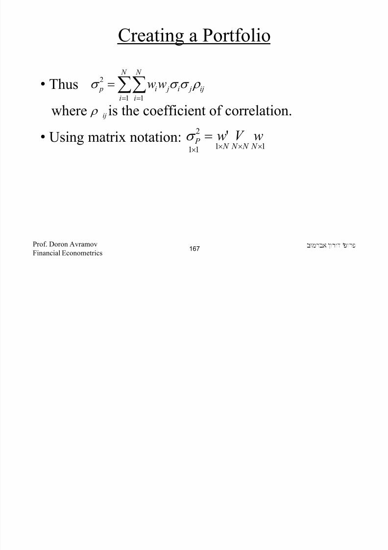
8/22/2019 Avramov Doron Financial Econometrics
http://slidepdf.com/reader/full/avramov-doron-financial-econometrics 167/553
where is the coefficient of correlation.• Using matrix notation:
1111
2 '××××
= N N N N
P wV wσ
ij ρ
'Prof. Doron Avramov
Financial Econometrics167
The Case of Two Risky Assets
• To illustrate, let us consider two risky assets:2211 Rw Rw R p +=
22222

8/22/2019 Avramov Doron Financial Econometrics
http://slidepdf.com/reader/full/avramov-doron-financial-econometrics 168/553
• We know:
• Let us check:
• So it works!
22122111 2 σ σ σ σ wwww RVAR pt p ++==
( ) 2
2
2
21221
2
1
2
1
2
1
2
212
12
2
1
21
2 2,,, σ σ σ σ σ σ σ σ wwww
wwww p ++=
=
'Prof. Doron Avramov
Financial Econometrics168
Dominance of the Covariance
• When the number of assets is large, the
covariances define the portfolio’s rate of return.

8/22/2019 Avramov Doron Financial Econometrics
http://slidepdf.com/reader/full/avramov-doron-financial-econometrics 169/553
• To illustrate, assume that all assets have the samevolatility and pairwise correlations.
• Then an equal weight portfolio’s variation is
cov)1( 2
2
22 =→
−+=
∞→
ρ σ ρ
σ σ N
p
N
N N N
'Prof. Doron Avramov
Financial Econometrics169
The Efficient Frontier: ExcludingRiskfree Asset
The optimization program:
min Vww'
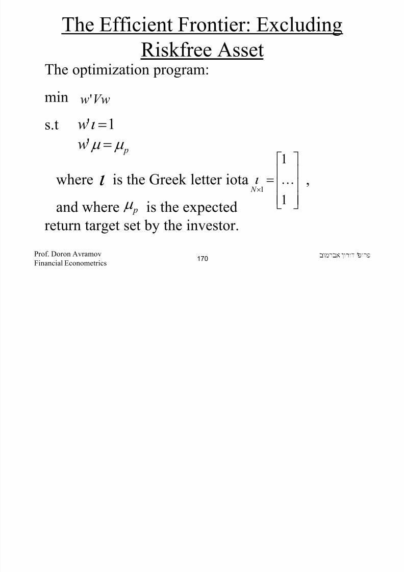
8/22/2019 Avramov Doron Financial Econometrics
http://slidepdf.com/reader/full/avramov-doron-financial-econometrics 170/553
s.t
where is the Greek letter iota ,
and where is the expected
return target set by the investor.
1' =ι w
pw µ µ ='
ι
=
×
1
1
1K
N ι
pµ
'Prof. Doron Avramov
Financial Econometrics170
The Efficient Frontier: Excluding
Riskfree AssetUsing the Lagrange setup:
1

8/22/2019 Avramov Doron Financial Econometrics
http://slidepdf.com/reader/full/avramov-doron-financial-econometrics 171/553
( ) ( )
µ λ ι λ
µ λ ι λ
µ µ λ ι λ
1
2
1
1
21
21
0
''1'2
1
−− +=
=−−=∂∂
−+−+=
V V w
Vww L
wwVww L p
'Prof. Doron Avramov
Financial Econometrics171
The Efficient Frontier: WithoutRiskfree Asset
• Let
ι ι
µ µ µ ι
1
1
1
'
''
−
−
−
=
==
V c
V bV a

8/22/2019 Avramov Doron Financial Econometrics
http://slidepdf.com/reader/full/avramov-doron-financial-econometrics 172/553
• The optimal portfolio is:
( )
( )ι µ
µ ι
11
11
2
1
1
−−
−−
−=
−=
−=
aV cV d
h
aV bV
d
g
abcd
p N N N
h g w µ 111
*
×
+=××
'Prof. Doron Avramov
Financial Econometrics172
Examine the Optimal Solution
• That is, once you specify the expected return target,
the optimal portfolio follows immediately.

8/22/2019 Avramov Doron Financial Econometrics
http://slidepdf.com/reader/full/avramov-doron-financial-econometrics 173/553
• Let us check whether the sum of weights is equal
to 1.
'Prof. Doron Avramov
Financial Econometrics173
Examine the Optimal Solution
( ) ( ) 1
1
''
1
'
'''
211
+=
−−
d
d
bdVVbd
h g w pµ ι ι ι

8/22/2019 Avramov Doron Financial Econometrics
http://slidepdf.com/reader/full/avramov-doron-financial-econometrics 174/553
Indeed, .
( ) ( )( ) ( ) 0
1''
1'
1'''
11 =−=−=
==−=−=−− acac
d
V aV c
d
h
d abcd V aV bd g
ι ι µ ι ι
µ ι ι ι ι
1' =ι w
'Prof. Doron Avramov
Financial Econometrics174
Examine the Optimal Solution
• Let us now check whether the expected return on
the portfolio is equal to .
R ll
pµ
h

8/22/2019 Avramov Doron Financial Econometrics
http://slidepdf.com/reader/full/avramov-doron-financial-econometrics 175/553
• Recall:
• So we need to show
( )µ µ µ µ
µ
''' h g w
h g w
p
p
+=+=
1'
0'
=
=
µ
µ
h
g
'Prof. Doron Avramov
Financial Econometrics175
Examine the Optimal Solution
( ) ( ) 01''1' 11 =−=−= −− ababd
V aV bd
g µ µ µ ι µ
8/22/2019 Avramov Doron Financial Econometrics
http://slidepdf.com/reader/full/avramov-doron-financial-econometrics 176/553
Try it yourself: prove that .1' =µ h
'Prof. Doron Avramov
Financial Econometrics176
Efficient Frontier The optimization program also delivers the shape of
the frontier.

8/22/2019 Avramov Doron Financial Econometrics
http://slidepdf.com/reader/full/avramov-doron-financial-econometrics 177/553
inefficient part
A
'Prof. Doron Avramov
Financial Econometrics177
Efficient Frontier
• Where point A stands for the Global Minimum
Variance Portfolio (GMVP).
8/22/2019 Avramov Doron Financial Econometrics
http://slidepdf.com/reader/full/avramov-doron-financial-econometrics 178/553
• The efficient frontier reflects the investment
opportunities; this is the supply side.
• Points below A are inefficient since they are being
dominated by other more attractive portfolios.
'Prof. Doron Avramov
Financial Econometrics178
The Notion of Dominance
If
AB
A B
µ µ
σ σ
≥
≤

8/22/2019 Avramov Doron Financial Econometrics
http://slidepdf.com/reader/full/avramov-doron-financial-econometrics 179/553
and there is at least one strong inequality, then portfolio B dominates portfolio A.
A B
'Prof. Doron Avramov
Financial Econometrics179
The Efficient Frontier with Riskfree
AssetIn practice, there is no really a riskfree asset. Why?
C dit i k

8/22/2019 Avramov Doron Financial Econometrics
http://slidepdf.com/reader/full/avramov-doron-financial-econometrics 180/553
• Credit risk.
• Inflation risk.
• Interest rate risk and the horizon effect.
'Prof. Doron Avramov
Financial Econometrics180
Setting the Optimization in the Presenceof Riskfree Asset
• The optimal solution is given by:
min
s t or
Vww'
( ) pfRww µιµ + '1' pef wR µµ+ '

8/22/2019 Avramov Doron Financial Econometrics
http://slidepdf.com/reader/full/avramov-doron-financial-econometrics 181/553
s.t or,
and the tangency portfolio takes the form:
• The tangency portfolio is investing all the funds in
risky assets.
( ) p f Rww µ ι µ =−+ 1 p f w R µ µ =+
( )( ) e
e
f
f
V V
RV RV w
µ ι µ
ι µ ι ι µ
1
1
1
1
*
'' −
−
−
−
=⋅−
⋅−=
'Prof. Doron Avramov
Financial Econometrics181
The Investment Opportunities• However, the investor could select any point in the
line emerging from the riskfree rate and touching the
efficient frontier in point T.

8/22/2019 Avramov Doron Financial Econometrics
http://slidepdf.com/reader/full/avramov-doron-financial-econometrics 182/553
• The location depends on the attitude toward risk.
T
'Prof. Doron Avramov
Financial Econometrics182
Fund Separation• Interestingly, all investors in the economy will mix
the tangency portfolio with a riskfree asset.• The mix depends on preferences.
• But the proportion of risky assets will be equal

8/22/2019 Avramov Doron Financial Econometrics
http://slidepdf.com/reader/full/avramov-doron-financial-econometrics 183/553
• But the proportion of risky assets will be equalacross the board.
• One way to test the CAPM is indeed to examinewhether all investors hold the same proportions of
risky assets.
• Obviously they don’t!
'Prof. Doron Avramov
Financial Econometrics183
General Equilibrium• The efficient frontier reflects the supply side.
• What about the demand?
• The demand side can be represented by a set of
indifference curves

8/22/2019 Avramov Doron Financial Econometrics
http://slidepdf.com/reader/full/avramov-doron-financial-econometrics 184/553
indifference curves.
'Prof. Doron Avramov
Financial Econometrics184
General Equilibrium• Why is the slope of indifference curve positive?
• The equilibrium obtains when the indifference
curve tangents the efficient frontier
• No riskfree asset:

8/22/2019 Avramov Doron Financial Econometrics
http://slidepdf.com/reader/full/avramov-doron-financial-econometrics 185/553
No riskfree asset:
A
'Prof. Doron Avramov
Financial Econometrics185
General EquilibriumWith riskfree asset:
A

8/22/2019 Avramov Doron Financial Econometrics
http://slidepdf.com/reader/full/avramov-doron-financial-econometrics 186/553
A
'Prof. Doron Avramov
Financial Econometrics186
Maximize Utility / Certainty
Equivalent ReturnIn the presence of a riskfree security, the tangency
point can be found by maximizing a utility functionf h f

8/22/2019 Avramov Doron Financial Econometrics
http://slidepdf.com/reader/full/avramov-doron-financial-econometrics 187/553
point can be found by maximizing a utility functionof the form
where is the relative risk aversion.
2
2
1 p pU γσ µ −=
γ
'Prof. Doron Avramov
Financial Econometrics187
Maximize Utility / Certainty
Equivalent Return• Notice that utility is equal to expected return minus
a penalty factor.

8/22/2019 Avramov Doron Financial Econometrics
http://slidepdf.com/reader/full/avramov-doron-financial-econometrics 188/553
a penalty factor.
• The penalty factor positively depends on the risk aversion (demand) and variance (supply).
'Prof. Doron Avramov
Financial Econometrics188
Utility Maximization( )
e
e
e
f
V w
Vww
U
Vwww RwU
µ γ
γ µ
γ µ
1* 1
0
'2
1'
−
=
=−=∂∂
⋅−+=

8/22/2019 Avramov Doron Financial Econometrics
http://slidepdf.com/reader/full/avramov-doron-financial-econometrics 189/553
Notice that here we get the same tangency portfolio
where reflects the fraction of weights invested in
risky assets. The rest is invested in the riskfree asset.
e
e
V V w
µ ι µ 1
1
*
' −
−
=*w
'Prof. Doron Avramov
Financial Econometrics189
Mixing the Risky and RiskfreeAssets
• So if then all funds (100%) areinvested in risky assets
eV w µ γ
1* 1 −=
eV µ ι γ 1' −=

8/22/2019 Avramov Doron Financial Econometrics
http://slidepdf.com/reader/full/avramov-doron-financial-econometrics 190/553
( )invested in risky assets.
• If then some fraction is invested in
riskfree asset.
• If then the investor borrows money
to leverage his/her equity position.
eV µ ι γ 1' −>
eV µ ι γ 1' −<
'Prof. Doron Avramov
Financial Econometrics190
The Exponential Utility Function
• The exponential utility function is of the form
where
• Notice that
( ) ( )W W U λ −−= exp 0>λ
( ) ( ) 0exp' >−= WWU λλ

8/22/2019 Avramov Doron Financial Econometrics
http://slidepdf.com/reader/full/avramov-doron-financial-econometrics 191/553
• That is, the marginal utility is positive but
diminishes with an increasing wealth.
( ) ( )
( ) ( ) 0exp''
0exp
2 <−−=
>=
W W U
W W U
λ λ
λ λ
'Prof. Doron Avramov
Financial Econometrics191
The Exponential Utility Function
• Indeed, the exponential preferences belong to the
λ =−='
''
U
U ARA

8/22/2019 Avramov Doron Financial Econometrics
http://slidepdf.com/reader/full/avramov-doron-financial-econometrics 192/553
, p p g
class of constant absolute risk aversion (CARA).
• For comparison, power preferences belong to the
class of constant relative risk aversion (CRRA).
'Prof. Doron Avramov
Financial Econometrics192
Exponential: The Optimization
Mechanism• The investor maximizes the expected value of the
exponential utility where the decision variable is theset of weights w and subject to the wealth evolution

8/22/2019 Avramov Doron Financial Econometrics
http://slidepdf.com/reader/full/avramov-doron-financial-econometrics 193/553
p yset of weights w and subject to the wealth evolution.
• That is
( )[ ]t t W W U E 1+w
max
t s. et f t t Rw RW W 11 '1 ++ ++='Prof. Doron Avramov
Financial Econometrics193
Exponential: The Optimization
Mechanism• Let us assume that V N R ee
t ,~1 µ +

8/22/2019 Avramov Doron Financial Econometrics
http://slidepdf.com/reader/full/avramov-doron-financial-econometrics 194/553
• Then
mean variance
( )[ ]VwwW w RW N W t
e
f t t ','1~ 2
1 µ +++
'Prof. Doron Avramov
Financial Econometrics194
Exponential: The Optimization
MechanismIt is known that for
2,~ x x N x σ µ

8/22/2019 Avramov Doron Financial Econometrics
http://slidepdf.com/reader/full/avramov-doron-financial-econometrics 195/553
( )[ ]
+=
22
2
1expexp x x aaax E σ µ
'Prof. Doron Avramov
Financial Econometrics195
Exponential: The Optimization
MechanismThus,
( )[ ] ( )( ) ( )
⋅+−−=−− +++ W VARW E W E t t t
21expexp 1
211 λ λ λ

8/22/2019 Avramov Doron Financial Econometrics
http://slidepdf.com/reader/full/avramov-doron-financial-econometrics 196/553
( )[ ] ( )( ) ( )
( )
( )( )
−−+−−=
+++−−=
VwwW wW RW
VwwW w RW
t
e
t f t
t
e
f t
'2
1
'exp1exp
'2
1'1exp
2
22
λ µ λ λ
λ µ λ
'Prof. Doron Avramov
Financial Econometrics196
Exponential: The Optimization
Mechanism Notice that
t W λ γ =

8/22/2019 Avramov Doron Financial Econometrics
http://slidepdf.com/reader/full/avramov-doron-financial-econometrics 197/553
where is the relative risk aversion coefficient.γ
'Prof. Doron Avramov
Financial Econometrics197
Exponential: The OptimizationMechanism
• So the investor ultimately maximizes
w
max
− Vwww e '2
1' γ µ

8/22/2019 Avramov Doron Financial Econometrics
http://slidepdf.com/reader/full/avramov-doron-financial-econometrics 198/553
• The optimal solution is .
• The tangency portfolio is the same as before
eV w µ γ
1* 1 −=
e
e
V
V
w µ ι
µ 1
1*
' −
−
=
'Prof. Doron Avramov
Financial Econometrics198
Exponential: The Optimization
MechanismConclusion:
The joint assumption of exponential utility and

8/22/2019 Avramov Doron Financial Econometrics
http://slidepdf.com/reader/full/avramov-doron-financial-econometrics 199/553
j p p y
normally distributed stock return leads to the well-
known mean variance solution.
'Prof. Doron Avramov
Financial Econometrics199
Quadratic Preferences
• The quadratic utility function is of the formwhere( ) 2
2W
bW aW U −+= 0>b
1−=∂∂ bW WU

8/22/2019 Avramov Doron Financial Econometrics
http://slidepdf.com/reader/full/avramov-doron-financial-econometrics 200/553
• Notice that the first derivative is positive for
02
2
<−=∂∂
∂
bW U
W
W
b1
<
'Prof. Doron Avramov
Financial Econometrics200
Quadratic Preferences
The utility function looks like( )W U
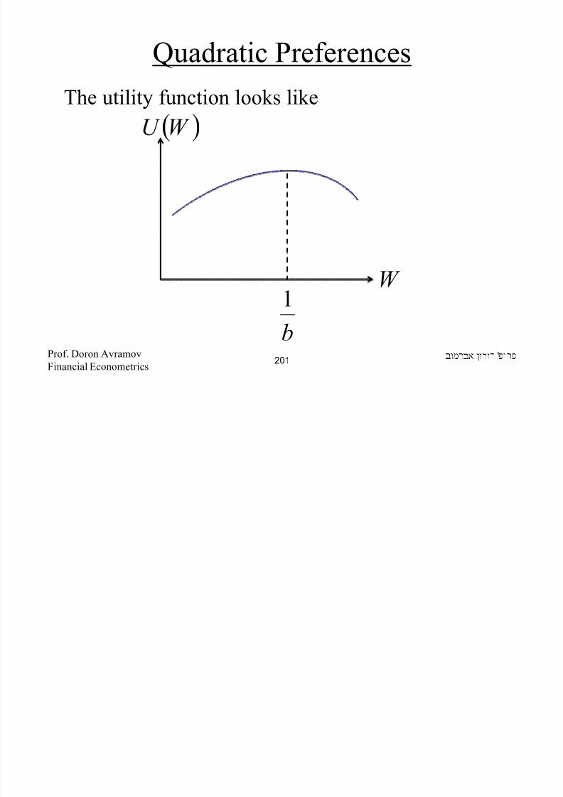
8/22/2019 Avramov Doron Financial Econometrics
http://slidepdf.com/reader/full/avramov-doron-financial-econometrics 201/553
W
b
1
'Prof. Doron Avramov
Financial Econometrics201
Quadratic Preferences
• It has a diminishing part – which makes no sense – because we always prefer higher than lower wealth
• Utility is thus restricted to the positive slope part
• Notice thatbW
WU
RRA ===''
γ

8/22/2019 Avramov Doron Financial Econometrics
http://slidepdf.com/reader/full/avramov-doron-financial-econometrics 202/553
• Notice that
• The optimization formulation is given by
bW W
U RRA
−=−==
1'γ
wmax
t s. et ft t t Rw RW W 11 '1 ++ ++=
( )[ ]t t W W U E 1+
'Prof. Doron Avramov
Financial Econometrics202
Quadratic Preferences
• Avramov and Chordia (2006 JFE ) show that theoptimization could be formulated as
( )wV w
R
w ee
ft
e 1''1
2
1'
−+
−
− µ µ µ w
max

8/22/2019 Avramov Doron Financial Econometrics
http://slidepdf.com/reader/full/avramov-doron-financial-econometrics 203/553
• The solution takes the form
( ) ft
γ
ee
e
ft
V
V Rw
µ µ
µ
γ
1'
1*
1
1−
−
+
−=
'Prof. Doron Avramov
Financial Econometrics203
Quadratic Preferences
• The tangency portfolio is
e
e
V
V
w µ ι
µ 1
1*
' −
−
=

8/22/2019 Avramov Doron Financial Econometrics
http://slidepdf.com/reader/full/avramov-doron-financial-econometrics 204/553
• The only difference from the previously presented
competing specifications is the composition of risky
and riskfree assets.
'Prof. Doron Avramov
Financial Econometrics204
The Sharpe Ratio of the TangencyPortfolio
• Notice that is actually the squaredSharpe Ratio of the tangency portfolio.
• Let us prove it
eeV µ µ 1' −
1*
eV µ−

8/22/2019 Avramov Doron Financial Econometrics
http://slidepdf.com/reader/full/avramov-doron-financial-econometrics 205/553
( )
( )21
1'
**'2
1
1'*'*'*'
1
*
'
'1
'
e
ee
TP
e
eee
f
e
f TP
e
V V wV w
V
V w Rww R
V
V w
µ ι µ µ σ
µ ι
µ µ µ ι µ µ
µ ι
µ
−
−
−
−
−
==
==−+=−
=
'Prof. Doron Avramov
Financial Econometrics205
The Sharpe Ratio of the Tangency
Portfolio
• Thus,
N ti th t TP i b i t f th t
( ) ee
TP
f TP
TP V R
SR µ µ σ
µ 1'
2
2
2 −=−
=

8/22/2019 Avramov Doron Financial Econometrics
http://slidepdf.com/reader/full/avramov-doron-financial-econometrics 206/553
• Notice that TP is a subscript for the tangency
portfolio.
'Prof. Doron Avramov
Financial Econometrics206
Lecture Notes in
Financial Econometrics

8/22/2019 Avramov Doron Financial Econometrics
http://slidepdf.com/reader/full/avramov-doron-financial-econometrics 207/553
Testing Asset Pricing Models:
Time Series Perspective
'Prof. Doron Avramov
Financial Econometrics207
Why Caring about Asset
Pricing Models?• An essential question that arises is why would both
academics and practitioners invest huge resources in
developing and testing asset pricing models.

8/22/2019 Avramov Doron Financial Econometrics
http://slidepdf.com/reader/full/avramov-doron-financial-econometrics 208/553
• It turns out that pricing models have crucial roles in
various applications in financial economics – bothasset pricing as well as corporate finance.
•In the following, I list five major applications.
'Prof. Doron Avramov
Financial Econometrics208
1 – Common Risk Factors
• Pricing models characterize the risk profile of a firm.
• In particular, systematic risk is no longer stock returnvolatility – rather it is the loadings on risk factors.

8/22/2019 Avramov Doron Financial Econometrics
http://slidepdf.com/reader/full/avramov-doron-financial-econometrics 209/553
y g
• For instance, in the single factor CAPM the market
beta – or the co-variation with the market –
characterizes the systematic risk of the firm.
'Prof. Doron Avramov
Financial Econometrics209
1 – Common Risk Factors
• Likewise, in the single factor (C)CAPM theconsumption growth beta – or the co-variation with
consumption growth – characterizes the systematic risk
of the firm.
• In the m lti factor Fama French (FF) model there are

8/22/2019 Avramov Doron Financial Econometrics
http://slidepdf.com/reader/full/avramov-doron-financial-econometrics 210/553
• In the multi-factor Fama-French (FF) model there are
three sources of risk – the market beta, the SMB beta,and the HML beta.
'Prof. Doron Avramov
Financial Econometrics210
1 – Common Risk Factors
• Under FF, other things being equal (ceteris paribus), afirm is riskier if its loading on SMB beta is higher.
• Under FF, other things being equal (ceteris paribus), a
firm is riskier if its loading on HML beta is higher.

8/22/2019 Avramov Doron Financial Econometrics
http://slidepdf.com/reader/full/avramov-doron-financial-econometrics 211/553
'Prof. Doron Avramov
Financial Econometrics211
2 – Moments for Asset
Allocation• Pricing models deliver moments for asset allocation.
• For instance, the tangency portfolio takes on the form

8/22/2019 Avramov Doron Financial Econometrics
http://slidepdf.com/reader/full/avramov-doron-financial-econometrics 212/553
e
e
TP V
V wµ ι µ 1
1
' −
−
=
'Prof. Doron Avramov
Financial Econometrics212
2 – Asset Allocation
Under the CAPM, the vector of expected returns and thecovariance matrix are given by:
e
m
e βµ µ =
∑+= 2' mV σ ββ

8/22/2019 Avramov Doron Financial Econometrics
http://slidepdf.com/reader/full/avramov-doron-financial-econometrics 213/553
where is the covariance matrix of the residuals in the
time-series asset pricing regression.
We denoted by the residual covariance matrix in the
case wherein the off diagonal elements are zeroed out.
∑
Ψ
'Prof. Doron Avramov
Financial Econometrics213
2 –Asset Allocation
The corresponding quantities under the FF model are
++= µ β µ β µ β µ HML HMLSMLSML
e
m MKT
e

8/22/2019 Avramov Doron Financial Econometrics
http://slidepdf.com/reader/full/avramov-doron-financial-econometrics 214/553
where is the covariance matrix of the factors.
∑+∑= ' β β F V
F ∑
'Prof. Doron Avramov
Financial Econometrics214
3 – Discount Factors
• Expected return is the discount factor, commonlydenoted by k , in present value formulas in general
and firm evaluation in particular:
( )∑=T
t
t
k
CF PV
1
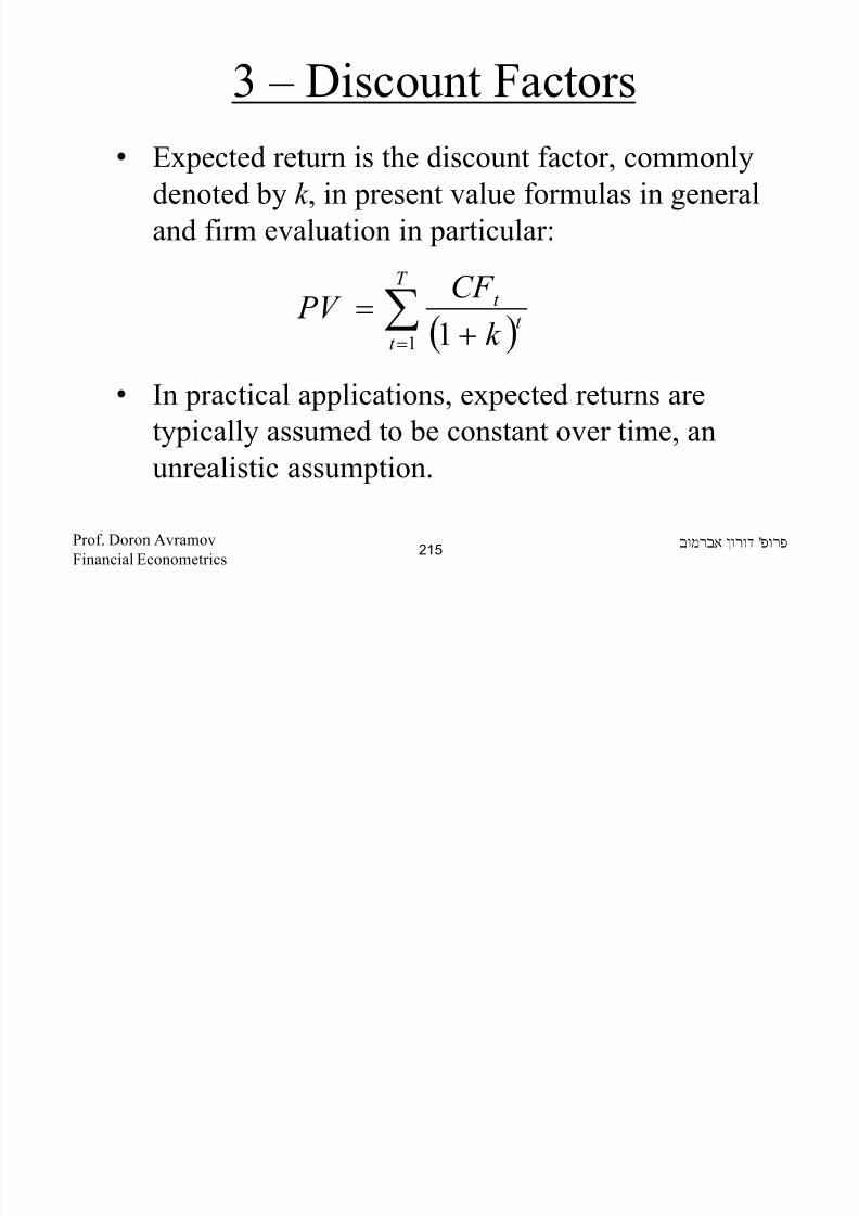
8/22/2019 Avramov Doron Financial Econometrics
http://slidepdf.com/reader/full/avramov-doron-financial-econometrics 215/553
• In practical applications, expected returns are
typically assumed to be constant over time, an
unrealistic assumption.
( )∑= +t
t k 1 1
'Prof. Doron Avramov
Financial Econometrics215
3 – Discount Factors• Indeed, thus far we have examined models with
constant beta and constant risk premiums
where is a K -vector of risk premiums.
Wh f t t d th i k i i
λ β µ '=e
λ
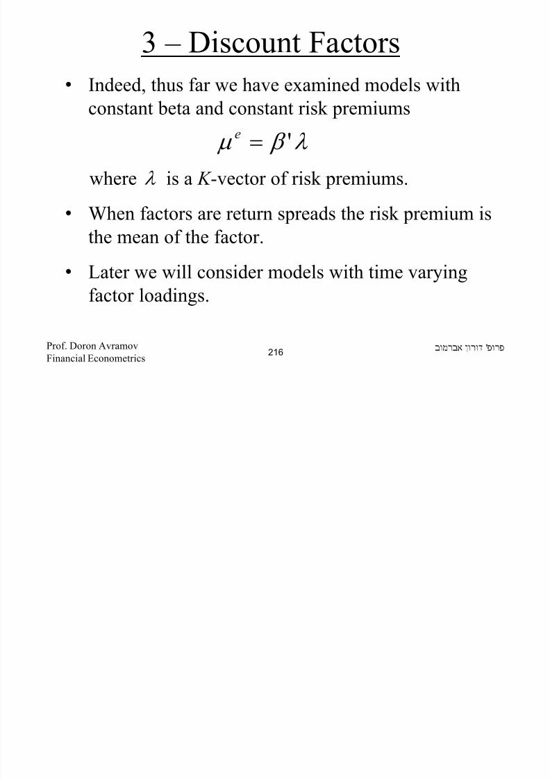
8/22/2019 Avramov Doron Financial Econometrics
http://slidepdf.com/reader/full/avramov-doron-financial-econometrics 216/553
• When factors are return spreads the risk premium is
the mean of the factor.
• Later we will consider models with time varying
factor loadings.
'Prof. Doron Avramov
Financial Econometrics216
4 – Benchmarks
• Factors in asset pricing models serve as benchmarksfor evaluating performance of active investments.
• In particular, performance is the intercept (alpha) in
the time series regression of excess fund returns on a
set of benchmarks (typically four benchmarks in
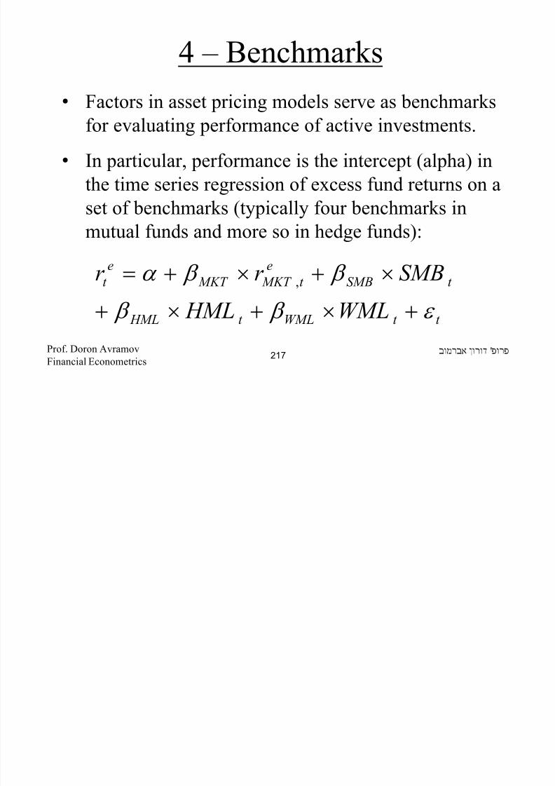
8/22/2019 Avramov Doron Financial Econometrics
http://slidepdf.com/reader/full/avramov-doron-financial-econometrics 217/553
set of benchmarks (typically four benchmarks in
mutual funds and more so in hedge funds):
t t WMLt HML
t SMB
e
t MKT MKT
e
t
WML HML
SMBr r
ε β β
β β α
+×+×+
×+×+= ,
'Prof. Doron Avramov
Financial Econometrics217
5 – Corporate Finance
• There is a plethora of studies in corporate finance thatuse asset pricing models to risk adjust asset returns.
• Here are several examples:
o Examining the long run performance of IPO firm.
8/22/2019 Avramov Doron Financial Econometrics
http://slidepdf.com/reader/full/avramov-doron-financial-econometrics 218/553
o Examining the long run performance of SEO firms.
o Analyzing abnormal performance of stocks going
through splits and reverse splits.
'Prof. Doron Avramov
Financial Econometrics218
5 – Corporate Finance
o Analyzing mergers and acquisitions
o Analyzing the impact of change in board of
directors.
o Studying the impact of corporate governance on
h i f

8/22/2019 Avramov Doron Financial Econometrics
http://slidepdf.com/reader/full/avramov-doron-financial-econometrics 219/553
the cross section of average returns.
o Studying the long run impact of stock/bond
repurchase.
'Prof. Doron Avramov
Financial Econometrics219
Time Series Tests
• Time series tests are designated to examine the validityof models in which factors are portfolio based, or
factors that are return spreads.
• Example: the market factor is the return difference
between the market portfolio and the riskfree asset.

8/22/2019 Avramov Doron Financial Econometrics
http://slidepdf.com/reader/full/avramov-doron-financial-econometrics 220/553
p
• Consumption growth is not a return spread.
• Thus, the consumption CAPM cannot be tested using
time series regressions, unless you form a factor
mimicking portfolio (FMP) for consumption growth.
'Prof. Doron Avramov
Financial Econometrics220
Time Series Tests• FMP is a convex combination of asset returns
having the maximal correlation with consumptiongrowth.
• The statistical time series tests have an appealingeconomic interpretation. In particular:

8/22/2019 Avramov Doron Financial Econometrics
http://slidepdf.com/reader/full/avramov-doron-financial-econometrics 221/553
• Testing the CAPM amounts to testing whether the
market portfolio is the tangency portfolio.
• Testing multi-factor models amounts to testing
whether some optimal combination of the factors isthe tangency portfolio.
'Prof. Doron Avramov
Financial Econometrics221
Testing the CAPM
• Run the time series regression:
ee
t
e
mt
e
t
rr
r r
εβα
ε β α
++=
++=
M
1111

8/22/2019 Avramov Doron Financial Econometrics
http://slidepdf.com/reader/full/avramov-doron-financial-econometrics 222/553
• The null hypothesis is:
Nt mt N N Nt r r ε β α ++=
0: 210 ==== N H α α α K
'Prof. Doron Avramov
Financial Econometrics222
Testing the CAPM
In the following, I will introduce four times series teststatistics:
• WALD.
• Likelihood Ratio.

8/22/2019 Avramov Doron Financial Econometrics
http://slidepdf.com/reader/full/avramov-doron-financial-econometrics 223/553
• GRS (Gibbons, Ross, and Shanken (1989)).
• GMM.
'Prof. Doron Avramov
Financial Econometrics223
The Distribution of .
• Recall, is asset mispricing.• The time series regressions can be rewritten using a
vector form as:
α
α
111111 NX t
X
e
mt NX NX NX
e
t r r ε β α +⋅+=

8/22/2019 Avramov Doron Financial Econometrics
http://slidepdf.com/reader/full/avramov-doron-financial-econometrics 224/553
• Let us assume that
for t=1,2,3,…,T
• Let be the set of all
parameters.
∑
NxN
iid
Nxt N ,0~1
ε
( )( )'',',' ε α θ vech=
'Prof. Doron Avramov
Financial Econometrics224
The Distribution of .
• Under normality, the likelihood function for is
α
( ) ( ) ( )
−−∑−−−∑=−−
e
mt
e
t
e
mt
e
t t r r r r c L β α β α θ ε 1'
2
1
2
1
exp
t ε

8/22/2019 Avramov Doron Financial Econometrics
http://slidepdf.com/reader/full/avramov-doron-financial-econometrics 225/553
where c is the constant of integration (recall theintegral of a probability distribution function is
unity).
'Prof. Doron Avramov
Financial Econometrics225
The Distribution of .
• Moreover, the IID assumption suggests that
α
( )
( ) ( )
−−∑−−−×
∑=
∑=
−
−
T
t
e
mt
e
t
e
mt
e
t
T
T
N
r r r r
c L
1
1'
221
2
1exp
,,,
β α β α
θ ε ε ε K

8/22/2019 Avramov Doron Financial Econometrics
http://slidepdf.com/reader/full/avramov-doron-financial-econometrics 226/553
• Taking the natural log from both sides yields
t
( ) ( ) ( ) ( )∑=
− −−∑−−−∑−∝T
t
e
mt
e
t
e
mt
e
t r r r r T
L
1
1'
2
1ln
2
ln β α β α
'Prof. Doron Avramov
Financial Econometrics226
The Distribution of .
Asymptotically, we have
where
α
( ))(,0~ˆ
θ θ θ Σ− N
( )1
2
'
ln−
∂∂−=Σ
θθ
α θ E

8/22/2019 Avramov Doron Financial Econometrics
http://slidepdf.com/reader/full/avramov-doron-financial-econometrics 227/553
' ∂∂ θ θ
'Prof. Doron Avramov
Financial Econometrics227
The Distribution of .
Let us estimate the parameters
α
( ) ( )
( ) ( )1
1
1
ln
ln
−
=
−
×−−∑=∂
−−∑=
∂
∂
∑∑
eT
ee
T
t
e
mt
e
t
rrr L
r r L
βα
β α
α

8/22/2019 Avramov Doron Financial Econometrics
http://slidepdf.com/reader/full/avramov-doron-financial-econometrics 228/553
( )
( ) 1
1
'11
1
2
1
2
ln −
=
−−
=
∑
∑+∑−=
∑∂∂
×∑=
∂
∑
∑T
t
t t
mt
t
mt t
T L
r r r
ε ε
β α
β
'Prof. Doron Avramov
Financial Econometrics228
The Distribution of .
Solving for the first order conditions yields
α
( )( )∑ −−
⋅−=T
e
m
e
mt
ee
t
e
m
e
r r ˆˆ
ˆˆˆˆ
µ µ
µ β µ α

8/22/2019 Avramov Doron Financial Econometrics
http://slidepdf.com/reader/full/avramov-doron-financial-econometrics 229/553
( )( )
( )∑
∑
=
=
−= T
t
e
m
e
mt
t
r 1
2
1
ˆˆ
µ β
'Prof. Doron Avramov
Financial Econometrics229
The Distribution of .
Moreover,
α
∑
∑=
=
=∑
T e
t
e
T
t
t t
r T
T 1
'
1ˆ
ˆˆ1ˆ
µ
ε ε

8/22/2019 Avramov Doron Financial Econometrics
http://slidepdf.com/reader/full/avramov-doron-financial-econometrics 230/553
∑
∑
=
=
=T
t
e
mt
e
m
t
t
r T
T
1
1
1µ
µ
'Prof. Doron Avramov
Financial Econometrics230
The Distribution of .
• Recall our objective is to find the variance-covariance matrix of .
• Standard errors could be found using the information
matrix.
α
α

8/22/2019 Avramov Doron Financial Econometrics
http://slidepdf.com/reader/full/avramov-doron-financial-econometrics 231/553
'Prof. Doron Avramov
Financial Econometrics231
The Distribution of .
• The information matrix is constructed as follows
α
( )
( ) ( ) ( )
( ) ( ) ( )
∂∂∂∑∂∂
∂
∂∂
∂
∂∂
∂
−=ln
,ln
,ln
'
ln,
'
ln,
'
ln
222
222
L L L
L L L
E I
α β α α α
θ

8/22/2019 Avramov Doron Financial Econometrics
http://slidepdf.com/reader/full/avramov-doron-financial-econometrics 232/553
( )
( ) ( ) ( )
∑∂∑∂∂
∂∑∂∂
∂∑∂∂ ∑∂∂∂∂∂∂
'
ln,
'
ln,
'
ln'
,
'
,
'222 L L L
β α
β β β α β
'Prof. Doron Avramov
Financial Econometrics232
The Distribution of the Parameters
• Try to establish yourself the information matrix.
• Notice that and are independent of -
thus, your can ignore the second derivatives withrespect to in the information matrix if your
objective is to find the distribution of and .
α
β
∑
∑α
β

8/22/2019 Avramov Doron Financial Econometrics
http://slidepdf.com/reader/full/avramov-doron-financial-econometrics 233/553
j
• If you aim to derive the distribution of then
focus on the bottom right block of the information
matrix.
β
'Prof. Doron Avramov
Financial Econometrics233
∑
The Distribution of .
• We get:
• Moreover,
α
∑
+2
ˆ
ˆ1
1,~ˆ
m
e
m
T N
σ
µ α α

8/22/2019 Avramov Doron Financial Econometrics
http://slidepdf.com/reader/full/avramov-doron-financial-econometrics 234/553
∑⋅ 2ˆ
11,~ˆmT
N σ
β β
( )∑−∑ ,2~ˆ T W T
'Prof. Doron Avramov
Financial Econometrics234
The Distribution of .
• Notice that W (x,y) stands for the Wishartdistribution with x=T-2 degrees of freedom and a
parameter matrix .
α
∑= y

8/22/2019 Avramov Doron Financial Econometrics
http://slidepdf.com/reader/full/avramov-doron-financial-econometrics 235/553
'Prof. Doron Avramov
Financial Econometrics235
The Wald Test
• Recall, if then
• Here we testwhere
( )∑,~ µ N X ( ) ( ) ( ) N X X 21 ~ˆ χ µ µ −∑− −
0ˆ:
0ˆ:
1
0
≠
=
α
α
H
H ( )α α ∑,0~ˆ
0
N H
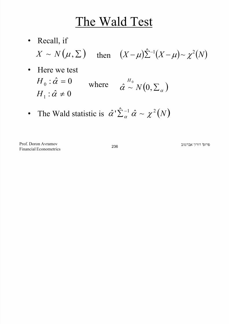
8/22/2019 Avramov Doron Financial Econometrics
http://slidepdf.com/reader/full/avramov-doron-financial-econometrics 236/553
• The Wald statistic is
0:1 ≠α H
( N 21 ~ˆˆ'ˆ χ α α α
−∑
'Prof. Doron Avramov
Financial Econometrics236
The Wald Test
which becomes:
2
11
12
1
ˆ1
ˆˆ'ˆˆˆ'ˆ
ˆ
ˆ1
mm
e
m
RS
T T J
+
∑=∑
+=
−−
−
α α α α
σ
µ
ˆ

8/22/2019 Avramov Doron Financial Econometrics
http://slidepdf.com/reader/full/avramov-doron-financial-econometrics 237/553
where is the Sharpe ratio of the market factor.m RS
'Prof. Doron Avramov
Financial Econometrics237
Algorithm for Implementation
• The algorithm for implementing the statistic is as
follows:
• Run separate regressions for the test assets on the
common factor:
11
121
21 TxxTxTx
e
t X r ε θ += ,1 1
e
mr
M
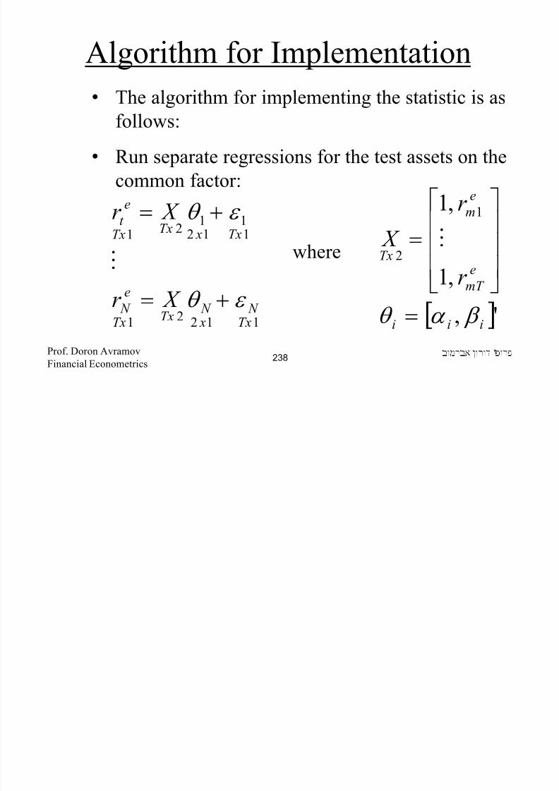
8/22/2019 Avramov Doron Financial Econometrics
http://slidepdf.com/reader/full/avramov-doron-financial-econometrics 238/553
where
11221
1121
Tx N
x N
TxTx
e
N
Tx xTx
X r ε θ +=
M
[ ]',
,12
iii
e
mT
Tx
r X
β α θ =
=M
'Prof. Doron Avramov
Financial Econometrics238
Algorithm for Implementation
• Retain the estimated regression intercepts
and
• Compute the residual covariance matrix
[ ]'ˆ,,ˆ,ˆˆ21 N α α α α K=
=
∧∧∧
N TxN
ε ε ε ,,1 K
∧∧
=∑ εε '1ˆ

8/22/2019 Avramov Doron Financial Econometrics
http://slidepdf.com/reader/full/avramov-doron-financial-econometrics 239/553
=∑ ε ε T
'Prof. Doron Avramov
Financial Econometrics239
Algorithm for Implementation
•Compute the sample mean and the sample variance
of the factor.•Compute J 1.

8/22/2019 Avramov Doron Financial Econometrics
http://slidepdf.com/reader/full/avramov-doron-financial-econometrics 240/553
'Prof. Doron Avramov
Financial Econometrics240
The Likelihood Ratio Test
• We run the unrestricted and restricted specifications:
un:
res:
t
e
mt
e
t r r ε β α ++=
**
t
e
mt
e
t r r ε β +=
( )∑,0~ N t ε
** ,0~ ∑ N t ε

8/22/2019 Avramov Doron Financial Econometrics
http://slidepdf.com/reader/full/avramov-doron-financial-econometrics 241/553
• Using MLE, we get:
'Prof. Doron Avramov
Financial Econometrics241
The Likelihood Ratio Test
( )
=∑
=
∑
∑
∑
=
=
=
'ˆˆ1ˆ
ˆ
1
***
1
2
1*
T
r
r r
T
t
t t
T
t
e
mt
T
t
e
mt
e
t
ε ε
β

8/22/2019 Avramov Doron Financial Econometrics
http://slidepdf.com/reader/full/avramov-doron-financial-econometrics 242/553
( )∑−∑
∑
+
,1~ˆ
ˆˆ
11,~ˆ
*
22
*
T W T
T N
mm σ µ β β
'Prof. Doron Avramov
Financial Econometrics242
The Likelihood Ratio Test
where again W is the Wishart distribution, this timewith T-1 degrees of freedom.

8/22/2019 Avramov Doron Financial Econometrics
http://slidepdf.com/reader/full/avramov-doron-financial-econometrics 243/553
'Prof. Doron Avramov
Financial Econometrics243
The LR Test
• Using some algebra, one can show that
( ) ( ) [ ][ ] ( ) N T LR J
T
L L LR
2*
2
**
~ˆlnˆln2
ˆln
ˆln2lnln
χ ∑−∑=−=
∑−∑−=−=
2 J
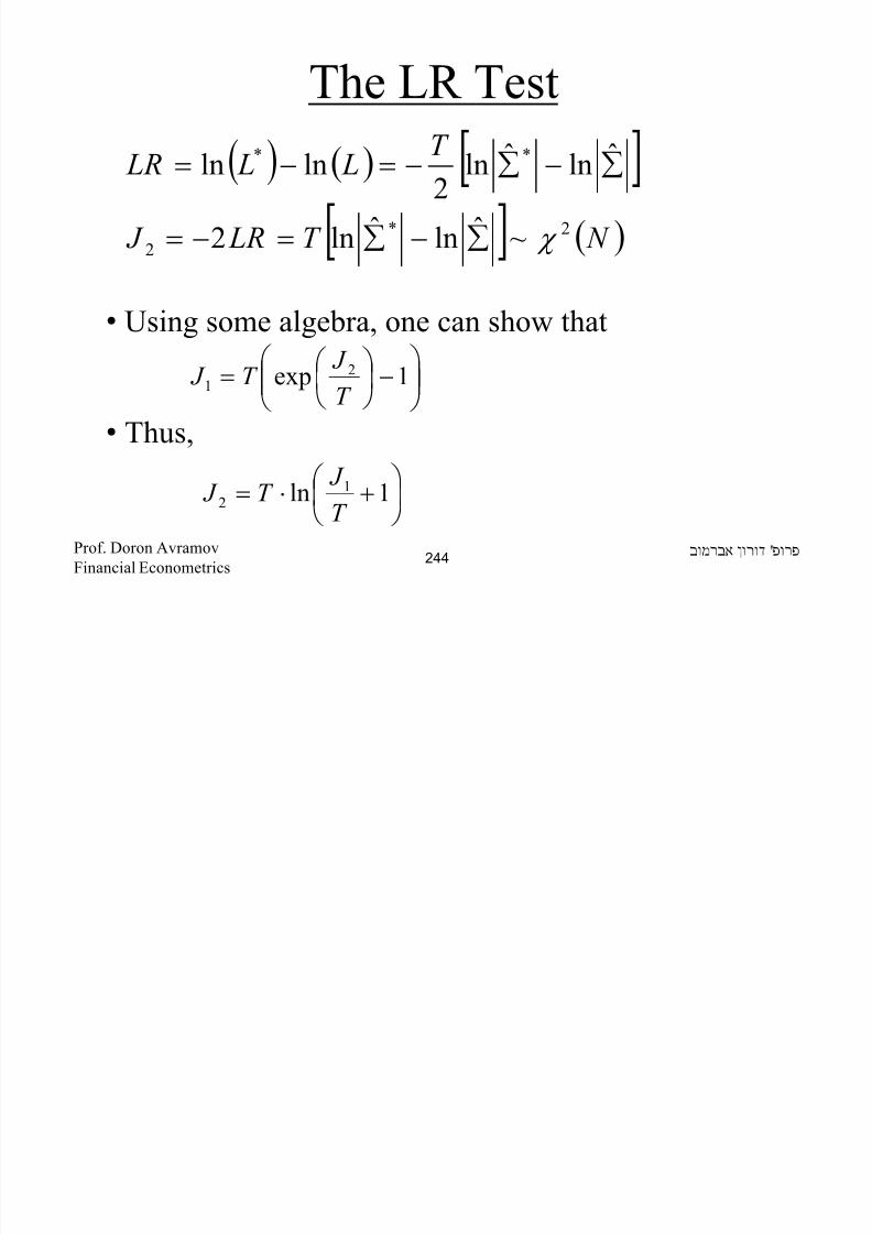
8/22/2019 Avramov Doron Financial Econometrics
http://slidepdf.com/reader/full/avramov-doron-financial-econometrics 244/553
• Thus, − = 1exp1 T T J
+⋅= 1ln
12
T
J T J
'Prof. Doron Avramov
Financial Econometrics244
GRS (1989)
Theorem: let
let where
and let A and X be independent then
( )∑,0~1
N X Nx
( )∑,~1
τ W A Nx
N ≥τ

8/22/2019 Avramov Doron Financial Econometrics
http://slidepdf.com/reader/full/avramov-doron-financial-econometrics 245/553
1,
1 ~'1
+−−+−
N N F X A X N
N τ
τ
'Prof. Doron Avramov
Financial Econometrics245
GRS (1989)
In our context:
( )
( )
2
,~
ˆ
,0~ˆˆˆ1
02
12
−=
∑∑=
∑
+=
−
T
whereW T A
N T X H
m
m
τ
τ
α σ µ
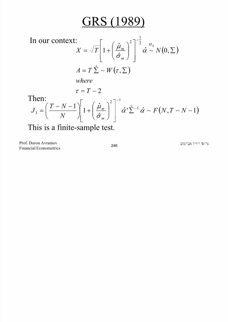
8/22/2019 Avramov Doron Financial Econometrics
http://slidepdf.com/reader/full/avramov-doron-financial-econometrics 246/553
Then:
This is a finite-sample test.
( )1,~ˆˆ'ˆˆ
ˆ1
1 1
12
3 −−∑
+
−−= −
−
N T N F N
N T J
m
m α α σ
µ
'Prof. Doron Avramov
Financial Econometrics246
GMM
I will directly give the statistic without derivation:
where
( )( ) )(~ˆ''ˆ 2111'
4
0
N R DS D RT J H
T T T χ α α ⋅=−−−
NxN NxN N
N Nx I R
=
20,

8/22/2019 Avramov Doron Financial Econometrics
http://slidepdf.com/reader/full/avramov-doron-financial-econometrics 247/553
( ) N
m
e
m
e
m
T I D ⊗
+
−=22
ˆˆ,ˆ
,1
σ µ µ
emµ ˆ
'Prof. Doron Avramov
Financial Econometrics247
GMM
• Assume no serial correlation but heteroskedasticity:
( )
[ ]'
1
''
,1
ˆˆ1
e
mt t
T
t
t t t t T
r x
where
x xT
S
=
⊗= ∑=
ε ε

8/22/2019 Avramov Doron Financial Econometrics
http://slidepdf.com/reader/full/avramov-doron-financial-econometrics 248/553
• Under homoskedasticity and serially uncorrelatedmoment conditions: J 4=J 1.
• That is, the GMM statistic boils down to the WALD.
'Prof. Doron Avramov
Financial Econometrics248
The Multi-Factor Version of Asset Pricing Tests
J 2 follows as described earlier.
( ) ( ) N T J
F r
F F F
Nxt
Kxt
NxK Nx Nx
et
χ α α µ µ
ε β α
~ˆˆ'ˆˆˆˆ1 11
1'
1
1111
−−
− ∑∑+=
+⋅+=

8/22/2019 Avramov Doron Financial Econometrics
http://slidepdf.com/reader/full/avramov-doron-financial-econometrics 249/553
where is the mean vector of the factor basedreturn spreads.
( ) ( ) K N T N F F F F N
K N T J −−−−− ∑∑+−−= ,
111'
3 ~ˆˆ'ˆˆˆˆ1 α α µ µ
F µ ˆ
'Prof. Doron Avramov
Financial Econometrics249
The Multi-Factor Version of Asset Pricing Tests
• is the variance covariance matrix of the factors.
•For instance, considering the Fama-French model:
eµ ˆ
F ∑
,,
2 ˆ,ˆ,ˆ HMLmSMBmm σ σ σ
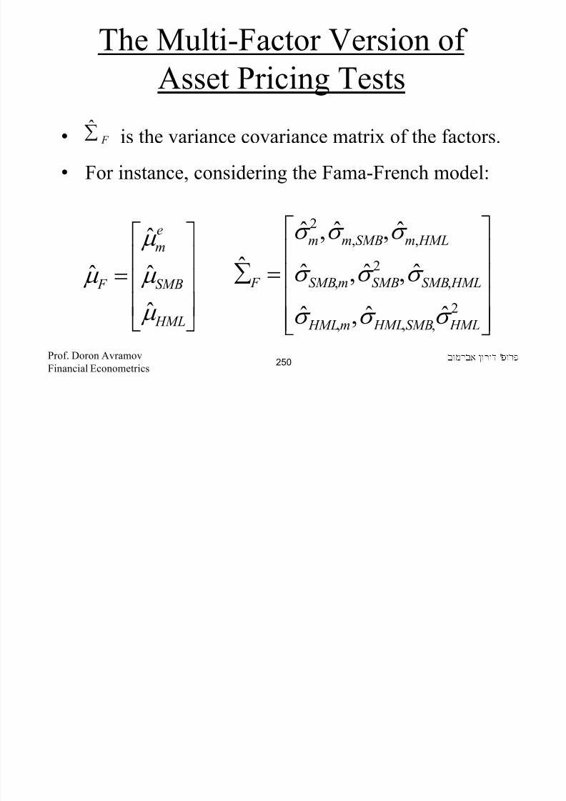
8/22/2019 Avramov Doron Financial Econometrics
http://slidepdf.com/reader/full/avramov-doron-financial-econometrics 250/553
=
HML
SMB
m
F
µ
µ
µ
µ
ˆ
ˆˆ
=∑2
,,,
,
2
,
ˆˆ,ˆ
ˆ,ˆ,ˆˆ
HMLSMB HMLm HML
HMLSMBSMBmSMB F
σ σ σ
σ σ σ
'Prof. Doron Avramov
Financial Econometrics250
The Current State of Asset PricingModels
o The CAPM has been rejected in asset pricing
tests.
o The Fama-French model is not a big success.
o Conditional versions of the CAPM and CCAPM

8/22/2019 Avramov Doron Financial Econometrics
http://slidepdf.com/reader/full/avramov-doron-financial-econometrics 251/553
display some improvement.
o Should decision-makers abandon a rejected
CAPM?
'Prof. Doron Avramov
Financial Econometrics251
Should a Rejected CAPM beAbandoned?
• Not necessarily!
• Assume that expected stock return is given by
where
• You estimate using the sample mean and CAPM:
f mi f ii R R −++= µ β α µ 0≠iα
iµ
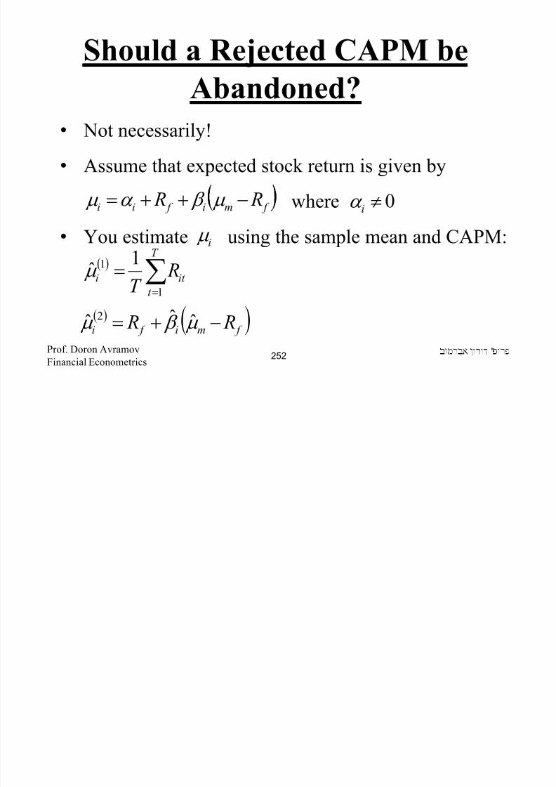
8/22/2019 Avramov Doron Financial Econometrics
http://slidepdf.com/reader/full/avramov-doron-financial-econometrics 252/553
g p
'Prof. Doron Avramov
Financial Econometrics252
( ) ∑=
=T
t
it i RT 1
1 1µ
( ) ( ) f mi f i R R −+= µ β µ ˆˆˆ 2
Mean Squared Error (MSE)
The quality of estimates is evaluated based on
the Mean Squared Error (MSE)
( ) ( )( )2
211 ˆii E MSE µ µ −=

8/22/2019 Avramov Doron Financial Econometrics
http://slidepdf.com/reader/full/avramov-doron-financial-econometrics 253/553
'Prof. Doron Avramov
Financial Econometrics253
( ) ( )( )22 ˆ ii E MSE µ µ −=
MSE, Bias, and Noise of Estimates
• Notice that
• Of course, the sample mean is unbiased thus
• However, the CAPM is rejected, thus
(
estimateVar bias MSE += 2
( ) ( )11 ˆiVar MSE µ =

8/22/2019 Avramov Doron Financial Econometrics
http://slidepdf.com/reader/full/avramov-doron-financial-econometrics 254/553
'Prof. Doron Avramov
Financial Econometrics254
( ) ( ))222 ˆii Var MSE µ α +=
The Bias-Variance Tradeoff
• It might be the case that is significantly
lower than - thus even when the CAPM is
rejected, still zeroing out could produce a smaller mean square error.
( )2ˆiVar µ
( )1ˆiVar µ
iα

8/22/2019 Avramov Doron Financial Econometrics
http://slidepdf.com/reader/full/avramov-doron-financial-econometrics 255/553
'Prof. Doron Avramov
Financial Econometrics255
When is the Rejected CAPM Superior?
( )( ) ( ) ( ) ( )[ ]
( )( ) ( )emii
imiii
Var Var
RT
RT
Var
µ β µ
ε σ σ β σ µ
ˆˆˆ
11ˆ
2
22221
=
+==

8/22/2019 Avramov Doron Financial Econometrics
http://slidepdf.com/reader/full/avramov-doron-financial-econometrics 256/553
'Prof. Doron Avramov
Financial Econometrics256
When is the Rejected CAPM Superior?Using variance decomposition
( )( )
( ) ( ) ( ) ( )
( )[ ]+=
+
=+
⋅=
+==
222
22
2
2
2
2
22
2
ˆ1
ˆ
ˆ
ˆ1ˆ
1
ˆ
ˆ
ˆ|ˆˆˆ|ˆˆ)ˆˆ(ˆ
miim
mi
m
e
mi
e
mi
m
ie
m
em
emi
em
emi
emii
h
SRT
T
E
T
Var
T
E
E
Var Var E Var Var
σ β ε σ
σ β
σ
µ ε σ µ β
σ
ε σ µ
µ µ β µ µ β µ β µ

8/22/2019 Avramov Doron Financial Econometrics
http://slidepdf.com/reader/full/avramov-doron-financial-econometrics 257/553
'Prof. Doron Avramov
Financial Econometrics257
=
2
2
ˆ
ˆ
m
e
mm E SR
where
σ
µ
When is the Rejected CAPM Superior?• Then
where is the R squared in the market regression.
Si i ll th ti f th i
( )( )( )( )
( )( )
( ) 22
2
222
1
2
1ˆ
ˆ R RSR
R
SR
Var
Var m
i
miim
i
i +−=+=σ
σ β ε σ
µ
µ
2 R
SR
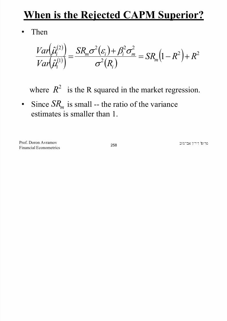
8/22/2019 Avramov Doron Financial Econometrics
http://slidepdf.com/reader/full/avramov-doron-financial-econometrics 258/553
• Since is small -- the ratio of the varianceestimates is smaller than 1.
'Prof. Doron Avramov
Financial Econometrics258
mSR
Example• Let
• For what values of it is sill preferred to use
th CAPM?
( )
3.0
05.0ˆ
ˆ
01.0
2
2
2
=
=
=
R
E
R
m
em
i
σ
µ
σ
0≠iα

8/22/2019 Avramov Doron Financial Econometrics
http://slidepdf.com/reader/full/avramov-doron-financial-econometrics 259/553
the CAPM?• Find such that the MSE of the CAPM is smaller.
'Prof. Doron Avramov
Financial Econometrics259
iα
Example
( )
( ) ( ) ( )
665001060
1
1
01.0601
3.07.005.0
11
2
2
1
222
1
2
<
⋅
++×
<++−=
i
i
im
MSE R RSR MSE
MSE
α
α
α

8/22/2019 Avramov Doron Financial Econometrics
http://slidepdf.com/reader/full/avramov-doron-financial-econometrics 260/553
'Prof. Doron Avramov
Financial Econometrics260
%528.101528.0
665.001.060
=<×⋅<
i
i
α
α
Economic versus StatisticalFactors
• Factors such as the market portfolio, SMB, HML,
WML, liquidity, credit risk, as well as bond based
factors are pre-specified.
• Such factors are considered to be economically
based

8/22/2019 Avramov Doron Financial Econometrics
http://slidepdf.com/reader/full/avramov-doron-financial-econometrics 261/553
based.
• For instance, Fama and French argue that SMB and
HML factors are proxying for underlying state
variables in the economy.'Prof. Doron Avramov
Financial Econometrics261
Economic versus StatisticalFactors
• Statistical factors are derived using econometric procedures on the covariance matrix of stock return.
• Two prominent methods are the factor analysis andthe principal component analysis (PCA).
• Such methods are used to extract common factors.

8/22/2019 Avramov Doron Financial Econometrics
http://slidepdf.com/reader/full/avramov-doron-financial-econometrics 262/553
• The first factor typically has a strong (about 96%)
correlation with the market portfolio.
• Later, I will explain the PCA.'Prof. Doron Avramov
Financial Econometrics262
The Economics of Time SeriesTest Statistics
Let us summarize the first three test statistics:
+⋅= 1ln 12
T
J T J
2
1
1
ˆ1
ˆˆ'ˆ
m RS
T J
+
∑=
− α α
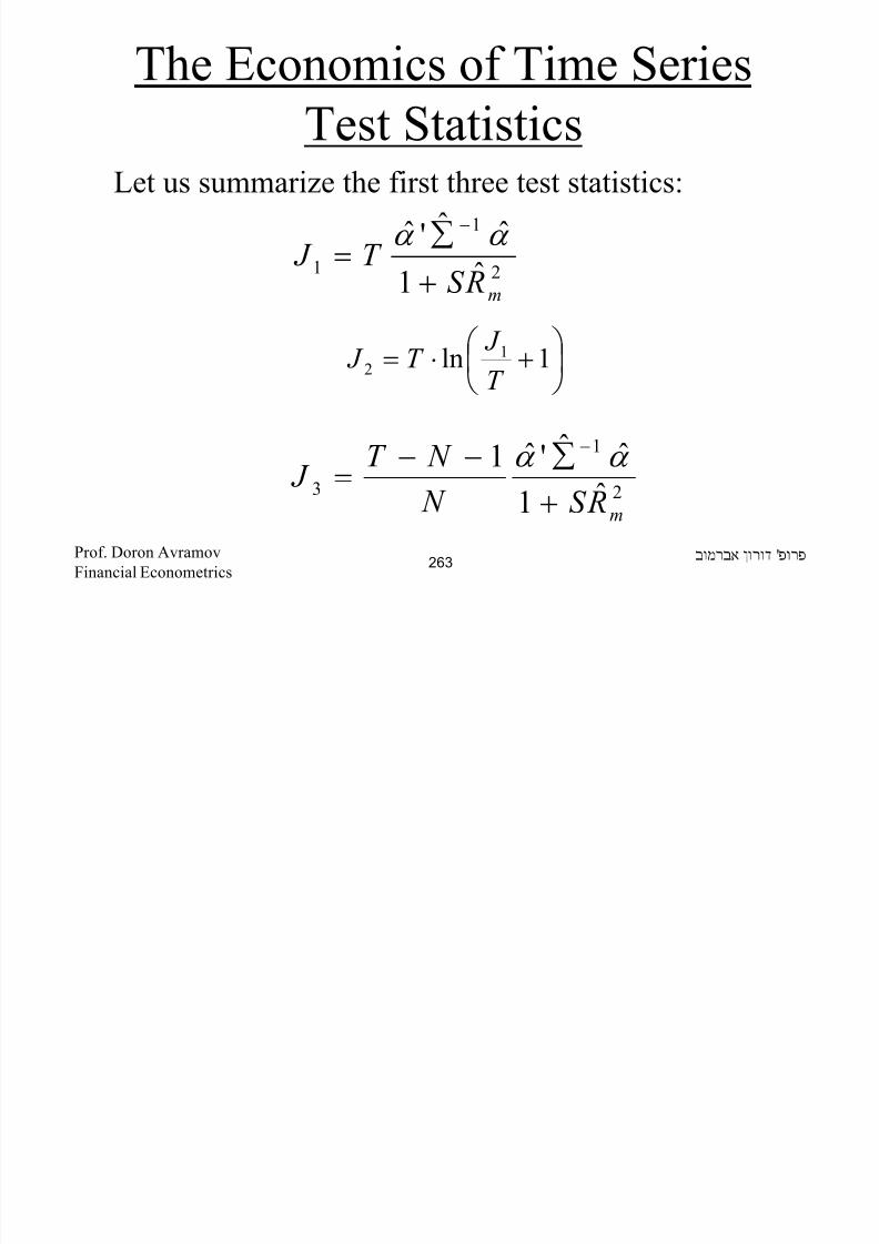
8/22/2019 Avramov Doron Financial Econometrics
http://slidepdf.com/reader/full/avramov-doron-financial-econometrics 263/553
2
1
3
ˆ1
ˆˆ'ˆ1
m RS N
N T J
+
∑−−=
− α α
'Prof. Doron Avramov
Financial Econometrics263
The Economics of the TimeSeries Tests
• The J 4 statistic, the GMM based asset pricing test, is
actually a Wald test, just like J 1, except that the
covariance matrix of asset mispricing takes accountof heteroskedasticity and often even potential serial
correlation.
• Notice that all test statistics depend on the quantity

8/22/2019 Avramov Doron Financial Econometrics
http://slidepdf.com/reader/full/avramov-doron-financial-econometrics 264/553
• Notice that all test statistics depend on the quantity
α α ˆˆ'ˆ 1−∑
'Prof. Doron Avramov
Financial Econometrics264
The Economics of the TimeSeries Tests
• GRS show that this quantity has a very insightful
representation.
• Let us provide the steps.

8/22/2019 Avramov Doron Financial Econometrics
http://slidepdf.com/reader/full/avramov-doron-financial-econometrics 265/553
'Prof. Doron Avramov
Financial Econometrics265
• Consider an investment universe that consists of N+1
assets - the N test assets as well as the market portfolio.
• The expected return vector of the N+1 assets is given
by
h i h i d d
( )''ˆ,ˆˆ
11111
=
+ xN
e
x
e
m x N
µ µ λ
eˆ
Understanding the Quantity .α α ˆˆ'ˆ1−
∑
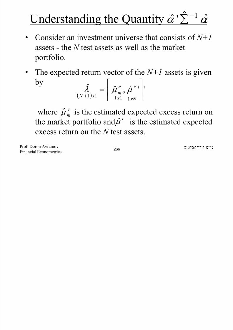
8/22/2019 Avramov Doron Financial Econometrics
http://slidepdf.com/reader/full/avramov-doron-financial-econometrics 266/553
where is the estimated expected excess return on
the market portfolio and is the estimated expected
excess return on the N test assets.
e
mµ ˆeµ ˆ
'Prof. Doron Avramov
Financial Econometrics266
• The variance covariance matrix of the N+1 assets is
given by
where
is the estimated variance of the market factor
( ) ( )
=Φ
++
V m
mm
N x N
ˆ,ˆˆ
ˆ'ˆ,ˆˆ
2
22
11
σ β
σ β σ
2
ˆ mσ
Understanding the Quantity .α α ˆˆ'ˆ1−
∑

8/22/2019 Avramov Doron Financial Econometrics
http://slidepdf.com/reader/full/avramov-doron-financial-econometrics 267/553
is the estimated variance of the market factor.
is the N -vector of market loadings and is the
covariance matrix of the N test assets.
mσ
β V
'Prof. Doron Avramov
Financial Econometrics267
• Notice that the covariance matrix of the N test assets
is
• The squared tangency portfolio of the N+1 assets is
∑+= ˆˆ'ˆˆˆ 2
mV σ β β
ˆˆˆˆ 12
Understanding the Quantity .α α ˆˆ'ˆ1−
∑

8/22/2019 Avramov Doron Financial Econometrics
http://slidepdf.com/reader/full/avramov-doron-financial-econometrics 268/553
λ λ ˆ'ˆ 12 −Φ=TP RS
'Prof. Doron Avramov
Financial Econometrics268
• Notice also that the inverse of the covariance matrix
is
• Thus, the squared Sharpe ratio of the tangency
( )
∑−
∑−∑+=Φ
−
−−−
−
β
β β β σ
ˆˆ
ˆ'ˆ,ˆˆ'ˆˆˆ
1
1112
1 m
1ˆ, −∑
Understanding the Quantity .α α ˆˆ'ˆ1−
∑

8/22/2019 Avramov Doron Financial Econometrics
http://slidepdf.com/reader/full/avramov-doron-financial-econometrics 269/553
Thus, the squared Sharpe ratio of the tangency portfolio could be represented as
'Prof. Doron Avramov
Financial Econometrics269
( ) ( )
221
122
1'
2
2
ˆˆˆˆ'ˆ
ˆˆ'ˆˆˆ
ˆˆˆˆˆˆˆˆˆˆ
mTP
e
m
ee
m
e
m
e
mTP
RSRS
or
RS RS
RS
∑
∑+=
−∑−+
=
−
−
−
αα
α α
µ β µ µ β µ σ µ
Understanding the Quantity .α α ˆˆ'ˆ1−
∑

8/22/2019 Avramov Doron Financial Econometrics
http://slidepdf.com/reader/full/avramov-doron-financial-econometrics 270/553
mTP RS RS −=∑ α α
'Prof. Doron Avramov
Financial Econometrics270
• In words, the quantity is the difference
between the squared Sharpe ratio based on the N+1assets and the squared Sharpe ratio of the market
portfolio.
• If the CAPM is correct then these two Sharpe ratios
are identical in population, but not identical in sample
due to estimation errors.
α α ˆˆ'ˆ 1−∑
Understanding the Quantity .α α ˆˆ'ˆ1−
∑
8/22/2019 Avramov Doron Financial Econometrics
http://slidepdf.com/reader/full/avramov-doron-financial-econometrics 271/553
due to estimation errors.
'Prof. Doron Avramov
Financial Econometrics271
• The test statistic examines how close the two sample
Sharpe ratios are.
• Under the CAPM, the extra N test assets do not add
anything to improving the risk return tradeoff.
• The geometric description of is given in
the next slide.α α ˆˆ'ˆ 1−∑
Understanding the Quantity .α α ˆˆ'ˆ1−
∑

8/22/2019 Avramov Doron Financial Econometrics
http://slidepdf.com/reader/full/avramov-doron-financial-econometrics 272/553
'Prof. Doron Avramov
Financial Econometrics272
1Φ
TP
2Φ Rf
r
σ
Understanding the Quantity .α α ˆˆ'ˆ1−
∑

8/22/2019 Avramov Doron Financial Econometrics
http://slidepdf.com/reader/full/avramov-doron-financial-econometrics 273/553
2
2
2
1
1 ˆˆ'ˆ Φ−Φ=∑ − α α
σ
'Prof. Doron Avramov
Financial Econometrics273
• So we can rewrite the previously derived test
statistics as
Understanding the Quantity .α α ˆˆ'ˆ1−
∑
( )
( )1,~ˆ
ˆˆ1
~
ˆ1
ˆˆ
2
22
3
2
2
22
1
−−−×−−=
+
−=
N T N F RS RS N T J
N
RS
RS RS T J
mTP
m
mTP χ

8/22/2019 Avramov Doron Financial Econometrics
http://slidepdf.com/reader/full/avramov-doron-financial-econometrics 274/553
( ),ˆ1 23
+×=
RS N m
'Prof. Doron Avramov
Financial Econometrics274
Asset Pricing Models withTime Varying Beta
• We consider for simplicity only the one factor
CAPM – extensions follow the same vein.
• Let us model beta variation with the lagged dividend
yield or any other macro variable – again for

8/22/2019 Avramov Doron Financial Econometrics
http://slidepdf.com/reader/full/avramov-doron-financial-econometrics 275/553
y y gsimplicity we consider only one information,
predictive, macro, or lagged variable.
'Prof. Doron Avramov
Financial Econometrics275
Asset Pricing Models withTime Varying Beta
• Typically, the set of predictive variables contains the
dividend yield, the term spread, the default spread,
the yield on a T-bill, inflation, lagged market return,
market volatility market illiquidity etc

8/22/2019 Avramov Doron Financial Econometrics
http://slidepdf.com/reader/full/avramov-doron-financial-econometrics 276/553
market volatility, market illiquidity, etc.
'Prof. Doron Avramov
Financial Econometrics276
Conditional Models
Here is a conditional asset pricing specification:
)|( 1
1
110
=
++=+=
++=
−
−
emt
emt
t t t
t iiit
it
e
mt it i
e
it
z r E
bz a z
z
r r
µ
η
β β β
ε β α
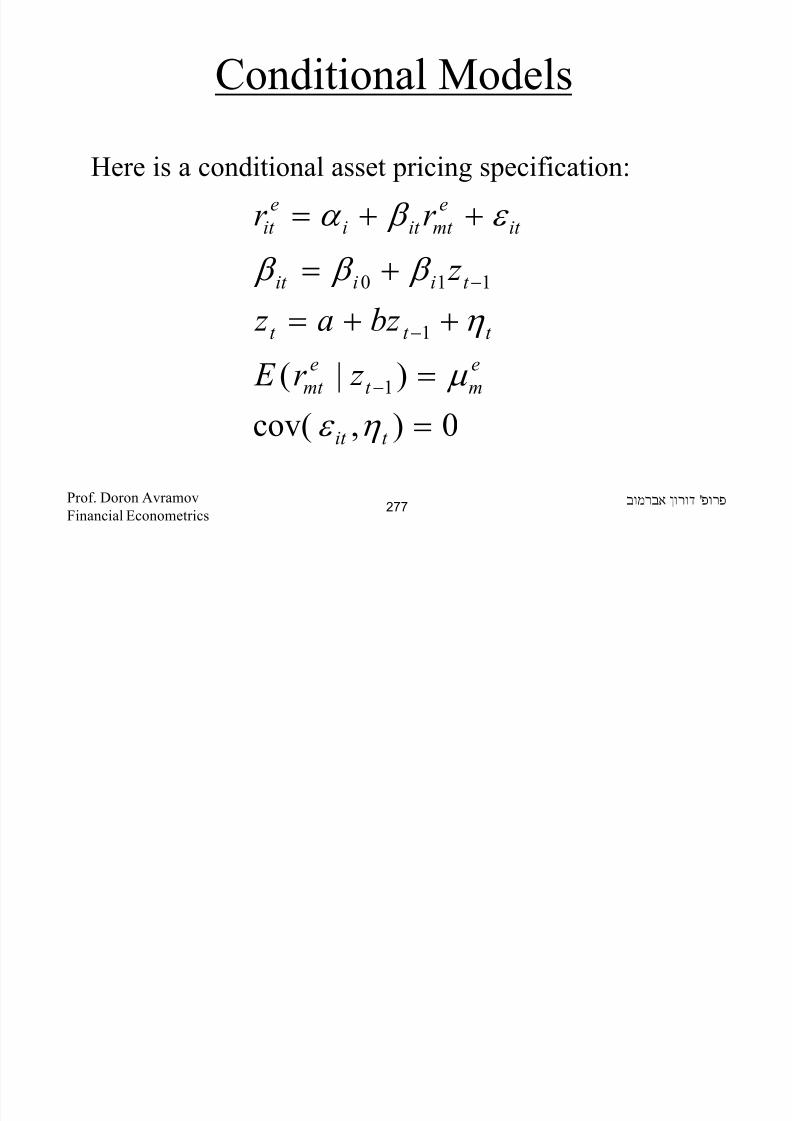
8/22/2019 Avramov Doron Financial Econometrics
http://slidepdf.com/reader/full/avramov-doron-financial-econometrics 277/553
0),cov(
)|( 1
=−
t it
mt mt
η ε
µ
'Prof. Doron Avramov
Financial Econometrics277
Conditional Asset PricingModels
• Substituting beta back into the asset pricing equation
yields.
• Interestingly, the one factor conditional CAPM
becomes a two factor unconditional model – the first
it t
e
mt i
e
mt ii
e
it z r r r ε β β α +++= −110

8/22/2019 Avramov Doron Financial Econometrics
http://slidepdf.com/reader/full/avramov-doron-financial-econometrics 278/553
factor is the market portfolio, while the second is the
interaction of the market with the lagged variable.'Prof. Doron Avramov
Financial Econometrics278
Conditional Asset PricingModels
• You can use the statistics J 1 through J 4 to test such
models.
• If we have K factors and M predictive variables then
the K -conditional factor model becomes a K+KM-
unconditional factor model.
If l l th k t b t i t i ll th

8/22/2019 Avramov Doron Financial Econometrics
http://slidepdf.com/reader/full/avramov-doron-financial-econometrics 279/553
• If you only scale the market beta, as is typically the
case, we have an M+K unconditional factor model.
'Prof. Doron Avramov
Financial Econometrics279
Conditional Moments
Suppose you are at time t – what is the discount factor
for time t+2?
2121202 +++++ +++= it t
e
mt i
e
mt ii
e
it z r r r ε β β α
( ) 212120 ++++ +++×++= it t t
e
mt i
e
mt ii bz ar r ε η β β α
+++++= eeee rzbrrar εηββββα

8/22/2019 Avramov Doron Financial Econometrics
http://slidepdf.com/reader/full/avramov-doron-financial-econometrics 280/553
2121212120 ++++++ +++++= it t mt it mt imt imt ii r z br r ar ε η β β β β α
'Prof. Doron Avramov
Financial Econometrics280
Conditional Moments
t
e
mi
e
mi
e
miit
e
it z ba z r E µ β µ β µ β α 1102 +++=+
( ) t
e
mi
e
miii z ba µ β µ β β α 110 +++=
• Notice that here the discount factor, or the conditional
expected return, is no longer constant through time.

8/22/2019 Avramov Doron Financial Econometrics
http://slidepdf.com/reader/full/avramov-doron-financial-econometrics 281/553
•Rather, it varies with the macro variable.
'Prof. Doron Avramov
Financial Econometrics281
Conditional Moments
Could you derive a general formula – in particular –
you are at time t what is the expected return for time
t+T as a function of the model parameters as well as
?
t z

8/22/2019 Avramov Doron Financial Econometrics
http://slidepdf.com/reader/full/avramov-doron-financial-econometrics 282/553
'Prof. Doron Avramov
Financial Econometrics282
Conditional Moments
• Next, the conditional covariance matrix – the
covariance at time t+1 given – is given by
where and are the N -asset versions of
[ ] ( )( ) Σ+++=+2'
10101 mt t t e
t z z z r V σ β β β β
0
β 1
β 0i
β
t z

8/22/2019 Avramov Doron Financial Econometrics
http://slidepdf.com/reader/full/avramov-doron-financial-econometrics 283/553
and respectively.1i β
'Prof. Doron Avramov
Financial Econometrics283
Conditional Moments
• Could you derive a general formula – in particular –
you are at time t what is the conditional covariance
matrix for time t+T as a function of the model
parameters as well as ?
• Could you derive general expressions for the
t z

8/22/2019 Avramov Doron Financial Econometrics
http://slidepdf.com/reader/full/avramov-doron-financial-econometrics 284/553
conditional moments of cumulative return?
'Prof. Doron Avramov
Financial Econometrics284
Conditional versusUnconditional Models
• There are different ways to model beta variation.
Here we used lagged predictive variables; other
applications include using firm level variables such
as size and book market to scale beta as well as

8/22/2019 Avramov Doron Financial Econometrics
http://slidepdf.com/reader/full/avramov-doron-financial-econometrics 285/553
modeling beta as an autoregressive process.
'Prof. Doron Avramov
Financial Econometrics285
Conditional versusUnconditional Models
• You can also model time variation in the risk
premiums in addition to or instead of beta variations.
• Asset pricing tests show that conditional models
typically outperform their unconditionalcounterparts

8/22/2019 Avramov Doron Financial Econometrics
http://slidepdf.com/reader/full/avramov-doron-financial-econometrics 286/553
counterparts.
'Prof. Doron Avramov
Financial Econometrics286
Different Ways to Model BetaVariation
• The base case: beta is constant, or time invariant.
• Case II: beta varies with macro conditions
t t t
t iiit
bz a z
z
ε
β β β
++=
+=
−
−
1
110

8/22/2019 Avramov Doron Financial Econometrics
http://slidepdf.com/reader/full/avramov-doron-financial-econometrics 287/553
'Prof. Doron Avramov
Financial Econometrics287
Different Ways to Model BetaVariation
• Case III: beta varies with firm-level size and the
book-to-market ratio
• Case IV: beta is some function of both macro and
firm-level variables as well as their interactions:
1,21,10 −− ++= t iit iiiit bm size β β β β
= bmsizezfβ

8/22/2019 Avramov Doron Financial Econometrics
http://slidepdf.com/reader/full/avramov-doron-financial-econometrics 288/553
1,1,1 ,, −−−= t it it it bm size z f β
'Prof. Doron Avramov
Financial Econometrics288
Different Ways to Model BetaVariation
Case V: beta follows an auto-regressive AR(1) process
it t iit vba ++= −1, β β

8/22/2019 Avramov Doron Financial Econometrics
http://slidepdf.com/reader/full/avramov-doron-financial-econometrics 289/553
'Prof. Doron Avramov
Financial Econometrics289
Single vs. Multiple Factors• Notice that we describe the case of a single factor
single macro variable.
• We can expand the specification to include more
factors and more macro and firm-level variables.
• Even if we expand the number of factors it is
common to model variation only in the market beta,
while the other risk loadings are constant.

8/22/2019 Avramov Doron Financial Econometrics
http://slidepdf.com/reader/full/avramov-doron-financial-econometrics 290/553
• Some scholars model time variations in all factor
loadings.'Prof. Doron Avramov
Financial Econometrics290
Testing Conditional Models• You can implement the J 1-J 4 test statistics only to
those cases where beta is either constant or it varieswith macro variables.
• Those specifications involving firm-levelcharacteristics require cross sectional tests.
• The last specification (AR(1)) requires filtering
methods involving state space representations.

8/22/2019 Avramov Doron Financial Econometrics
http://slidepdf.com/reader/full/avramov-doron-financial-econometrics 291/553
'Prof. Doron Avramov
Financial Econometrics291
Lecture Notes in
Financial Econometrics
GMVP and Tracking ErrorVolatility

8/22/2019 Avramov Doron Financial Econometrics
http://slidepdf.com/reader/full/avramov-doron-financial-econometrics 292/553
'Prof. Doron Avramov
Financial Econometrics292
GMVP
• Of particular interest to academics and practitioners isthe Global Minimum Volatility Portfolio.
• For two distinct reasons:
1. No need to estimate the notoriously difficult to
estimate .
2. Low volatility stocks have been found to
t f hi h l tilit t k
µ

8/22/2019 Avramov Doron Financial Econometrics
http://slidepdf.com/reader/full/avramov-doron-financial-econometrics 293/553
outperform high volatility stocks.
'Prof. Doron Avramov
Financial Econometrics293
GMVP Optimization
min
s.t
• Solution:
• No analytical solution in the presence of portfolio
Vww'
1' =ι w
ι ι
ι 1
1
' −
−
=V
V wGMVP

8/22/2019 Avramov Doron Financial Econometrics
http://slidepdf.com/reader/full/avramov-doron-financial-econometrics 294/553
• No analytical solution in the presence of portfolio
constraints –such as no short selling.'Prof. Doron Avramov
Financial Econometrics294
GMVP Optimization
• Ex ante, the GMVP is the lowest volatility portfolioamong all efficient portfolios.
• Ex ante, it is also the lowest mean portfolio, but ex
post it performs reasonably well in delivering high
payoffs.
8/22/2019 Avramov Doron Financial Econometrics
http://slidepdf.com/reader/full/avramov-doron-financial-econometrics 295/553
'Prof. Doron Avramov
Financial Econometrics295
The Tracking Error Volatility(TEV) Portfolio
• Actively managed funds are often evaluated based on
their ability to achieve high return subject to some
constraint on their Tracking Error Volatility (TEV).
• In that context, a managed portfolio can be
decomposed into both passive and active components.
• TEV is the volatility of the active component.

8/22/2019 Avramov Doron Financial Econometrics
http://slidepdf.com/reader/full/avramov-doron-financial-econometrics 296/553
'Prof. Doron Avramov
Financial Econometrics296
The Tracking Error Volatility(TEV) Portfolio
• The passive component is the benchmark portfolio.
• The benchmark portfolio changes with the
investment objective.
• For instance, if you invest in TA 100 stocks the
proper benchmark would be the TA100 index.• If you invest in corporate bonds traded in TASE the

8/22/2019 Avramov Doron Financial Econometrics
http://slidepdf.com/reader/full/avramov-doron-financial-econometrics 297/553
If you invest in corporate bonds traded in TASE the
benchmark could be TelBond 60.
'Prof. Doron Avramov
Financial Econometrics297
Tracking Error Volatility: TheBenchmark and Active Portfolios
• Let q be the vector of weights of the benchmark
portfolio.
• Then the expected return and variance of the benchmark portfolio are given by
where, as usual, µ and V are the vector of expected
Vqq
q
B
B
'
'
2
=
=
σ
µ µ

8/22/2019 Avramov Doron Financial Econometrics
http://slidepdf.com/reader/full/avramov-doron-financial-econometrics 298/553
, , µ p
return and the covariance matrix of stock returns.
'Prof. Doron Avramov
Financial Econometrics298
Tracking Error Volatility: TheBenchmark and Active Portfolios
• The matrix can be estimated in different methods –
most prominent of which will be discussed here.
• The active fund manager attempts to outperform this benchmark.
• Let x be the vector of deviations from the benchmark,or the active part of the managed portfolio.
V
8/22/2019 Avramov Doron Financial Econometrics
http://slidepdf.com/reader/full/avramov-doron-financial-econometrics 299/553
• Of course, the sum of all the components of x, by
construction, must be equal to zero.'Prof. Doron Avramov
Financial Econometrics299
The Mathematics of TEV• So the fund manager invests w=q+x in stocks, q is the
passive part of the portfolio and x is the active part.
• Notice that is the tracking error variance.
• Also notice that the expected return and volatility of
the chosen portfolio are
Vx x'2 =ξ σ
222
'2
'
ξ σ σ σ
µ µ µ
++=
+=
Vxw
x
B p
B p

8/22/2019 Avramov Doron Financial Econometrics
http://slidepdf.com/reader/full/avramov-doron-financial-econometrics 300/553
'Prof. Doron Avramov
Financial Econometrics300
The Mathematics of TEV• The optimization problem is formulated as
ϑ
ι
µ
=
=
Vx
xt s
x x
'
0'..
'max

8/22/2019 Avramov Doron Financial Econometrics
http://slidepdf.com/reader/full/avramov-doron-financial-econometrics 301/553
'Prof. Doron Avramov
Financial Econometrics301
The Mathematics of TEVThe resulting active part of the portfolio, x, is given by
where
−±= − ι µ ϑ
c
aV
e x 1
cV
aV
bV
=
==
−
−
−
'
'
'
2
1
1
1
ι ι
ι µ
µ µ

8/22/2019 Avramov Doron Financial Econometrics
http://slidepdf.com/reader/full/avramov-doron-financial-econometrics 302/553
ecba =− /2
'Prof. Doron Avramov
Financial Econometrics302
Questions• Is the sum of the x components equal to zero?
• Prove that if the benchmark is the GMVP then all x
components are equal to zero.
• What if the benchmark is another efficient portfolio – does this result still hold?
• Does the active part of the portfolio depend on the benchmark composition?

8/22/2019 Avramov Doron Financial Econometrics
http://slidepdf.com/reader/full/avramov-doron-financial-econometrics 303/553
'Prof. Doron Avramov
Financial Econometrics303
Caveats about the Minimum TEVPortfolio
• Richard Roll (distinguished UCLA professor) points
out that the solution is independent on the benchmark.
• Put differently, the active part of the portfolio x is
totally independent of the passive part q.
• Of course, the overall portfolio q+x is impacted by q.
• The unexpected result is that the active manager paysno attention to the assigned benchmark. So it does not

8/22/2019 Avramov Doron Financial Econometrics
http://slidepdf.com/reader/full/avramov-doron-financial-econometrics 304/553
really matter if the benchmark is S&P or any other
index.'Prof. Doron Avramov
Financial Econometrics304
TEV with total VolatilityConstraint (based on Jorion – an Expert in
Risk Management)
• Given the drawbacks underlying the TEV portfolio we
add one more constraint on the total portfolio volatility.
• The derived active portfolio displays two advantages.
• First, its composition does depend on the benchmark.
• Second, the systematic volatility of the portfolio is
controlled by the investor

8/22/2019 Avramov Doron Financial Econometrics
http://slidepdf.com/reader/full/avramov-doron-financial-econometrics 305/553
controlled by the investor.
'Prof. Doron Avramov
Financial Econometrics305
TEV with total volatilityconstraint
• The optimization is formulated as
• Home assignment: deri e the optimal sol tion
2)()'(
'
0'..
'max
p
x
xqV xq
Vx x
xt s
x
σ
ϑ
ι
µ
=++
=
=
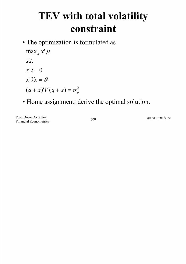
8/22/2019 Avramov Doron Financial Econometrics
http://slidepdf.com/reader/full/avramov-doron-financial-econometrics 306/553
• Home assignment: derive the optimal solution.
'Prof. Doron Avramov
Financial Econometrics306
Lecture Notes in
Financial Econometrics
Estimating the Large ScaleCovariance Matrix

8/22/2019 Avramov Doron Financial Econometrics
http://slidepdf.com/reader/full/avramov-doron-financial-econometrics 307/553
'Prof. Doron Avramov
Financial Econometrics307
Estimating the CovarianceMatrix:
• There are various applications in financial economics
which use the covariance matrix as an essential input.
• The Global Minimum Variance Portfolio, theminimum tracking error volatility portfolio, the mean
variance efficient frontier, and asset pricing tests are
good examples.
• In what follows I will present the most prominent

8/22/2019 Avramov Doron Financial Econometrics
http://slidepdf.com/reader/full/avramov-doron-financial-econometrics 308/553
w o ows w p ese e os p o e
estimation methods of the covariance matrix.'Prof. Doron Avramov
Financial Econometrics308
The Sample Covariance Matrix
(Denoted S )
•This method uses sample estimates.• Need to estimate N(N+1)/2 parameters which is a lot.
• You can use excel to estimate all variances and co-variances which is tedious and inefficient.
• Here is a much more efficient method.
• Consider T monthly returns on N risky assets.

8/22/2019 Avramov Doron Financial Econometrics
http://slidepdf.com/reader/full/avramov-doron-financial-econometrics 309/553
• We can display those returns in a T by N matrix R.'Prof. Doron Avramov
Financial Econometrics309
• Estimate the mean return of the N assets – and denote
the N -vector of the mean estimates by .
• Next, compute the deviations of the return
observations from their sample means:
where is a T vector of ones. Then the samplecovariance matrix is estimated as
∧
µ
∧∧
−= 'µ ι T R E
T ι ∧∧
= E E S '1
The Sample Covariance Matrix
(Denoted S )

8/22/2019 Avramov Doron Financial Econometrics
http://slidepdf.com/reader/full/avramov-doron-financial-econometrics 310/553
T
'Prof. Doron Avramov
Financial Econometrics310
The Equal Correlation BasedCovariance Matrix (Denoted F ):
• Estimate all N(N-1)/2 pair-wise correlations betweenany two securities and take the average.
• Let be that average correlation, let be theestimated variance of asset i, and let be the
estimated variance of asset j, both estimates are the i-th
and j-th elements of the diagonal of S .• Then the matrix F follows as
ρ ii s jj s
ii sii F =),(

8/22/2019 Avramov Doron Financial Econometrics
http://slidepdf.com/reader/full/avramov-doron-financial-econometrics 311/553
jjii s s ji F
−
= ρ ),('Prof. Doron Avramov
Financial Econometrics311
The Factor Based CovarianceMatrix:
• Consider the time series regression
where is an N vector of returns at time t and
is a set of K factors. Factor means are denoted by
• Notice that the mean return is given by
t t t e F r +×+= β α
t r
Fµβαµ ×+=
t F
F µ

8/22/2019 Avramov Doron Financial Econometrics
http://slidepdf.com/reader/full/avramov-doron-financial-econometrics 312/553
F µ β α µ ×+
'Prof. Doron Avramov
Financial Econometrics312
The Factor Based CovarianceMatrix
• Thus deviations from the means are given by
• The factor based covariance matrix is estimated by
Here, is an N by K matrix of factor loadings and
is a diagonal matrix with each element represents the
t F t t e F r +−×=− )( µ β µ
∧∧∧∧
Ψ+Σ= ' β β FF V
∧ β Ψ

8/22/2019 Avramov Doron Financial Econometrics
http://slidepdf.com/reader/full/avramov-doron-financial-econometrics 313/553
idio syncratic variance of each of the assets.
'Prof. Doron Avramov
Financial Econometrics313
The Factor Based CovarianceMatrix – Number of Parameters
• This procedure requires the estimation of NK betas aswell as K variances of the factors, K(K-1)/2
correlations of those factors, and N firm specific
variances.
• Overall, you need to estimate NK+K+K(K-1)/2+N
parameters, which is considerably less than N(N+1)/2
since K is much smaller than N .
• For instance using a single factor model – the number

8/22/2019 Avramov Doron Financial Econometrics
http://slidepdf.com/reader/full/avramov-doron-financial-econometrics 314/553
For instance, using a single factor model the number
of parameters to be estimated is only 2N+1.'Prof. Doron Avramov
Financial Econometrics314
Steps for Estimating the Factor Based Covariance Matrix
1) Run the MULTIVARIATE regression of stock
returns on asset pricing factors
where
( ) ( ) N T N K K T N T N K K T N T N T E F E F R
××++×××××××+⋅=++=
1111''' θ β α ι (
[ ][ ] β α θ
ι
,
,
=
= F F T (

8/22/2019 Avramov Doron Financial Econometrics
http://slidepdf.com/reader/full/avramov-doron-financial-econometrics 315/553
[ ]β,
'Prof. Doron Avramov
Financial Econometrics315
Steps for Estimating the Factor Based Covariance Matrix
2) Estimate
and retain only.
( )[ ] ( ) [ ] β α θ ˆ,ˆ''''ˆ
1'1
===
−−
F F F R R F F F
((((((
θ
β
)

8/22/2019 Avramov Doron Financial Econometrics
http://slidepdf.com/reader/full/avramov-doron-financial-econometrics 316/553
'Prof. Doron Avramov
Financial Econometrics316
Steps for Estimating the Factor Based Covariance Matrix
3) Estimate the covariance matrix of E
4) Let be a diagonal matrix with the
component being equal to the component
of .
N T T N N N E E T ××× =∆ '
1ˆ
( ) thii −,
( ) thii −,
∆
∧
Ψ

8/22/2019 Avramov Doron Financial Econometrics
http://slidepdf.com/reader/full/avramov-doron-financial-econometrics 317/553
'Prof. Doron Avramov
Financial Econometrics317
Steps for Estimating the Factor Based Covariance Matrix
5) Compute:
where is the mean return of the factors.
6) Estimate:
K
f T K T K T
F V ×
××× ⋅−=1
'
1µ ι
f µ ˆ
K T T K K K F V V
T ×××
⋅=∑ '1ˆ

8/22/2019 Avramov Doron Financial Econometrics
http://slidepdf.com/reader/full/avramov-doron-financial-econometrics 318/553
'Prof. Doron Avramov
Financial Econometrics318
Steps for Estimating the Factor Based Covariance Matrix
7)
This is the estimated covariance matrix of stock
returns.
8) Notice – there is no need to run N individual
regressions! Use multivariate specifications
∧
×××××
∧Ψ+∑=
N N N K K K F
K N N N V 'ˆˆˆ β β

8/22/2019 Avramov Doron Financial Econometrics
http://slidepdf.com/reader/full/avramov-doron-financial-econometrics 319/553
regressions! Use multivariate specifications.
'Prof. Doron Avramov
Financial Econometrics319
A Shrinkage Approach - Based ona Paper by Ledoit and Wolf (LW)
• There is a well perceived paper (among Wall Street
quants) by LW demonstrating an alternative approach
to estimating the covariance matrix.• It had been claimed to deliver superior performance in
reducing tracking errors relative to benchmarks as well
as producing higher Sharpe ratios.
• Here are the formal details.

8/22/2019 Avramov Doron Financial Econometrics
http://slidepdf.com/reader/full/avramov-doron-financial-econometrics 320/553
'Prof. Doron Avramov
Financial Econometrics320
A Shrinkage Approach - Based ona Paper by Ledoit and Wolf (LW)
• Let S be the sample covariance matrix, let F be the
equal correlation based covariance matrix, and let δ be
the shrinkage intensity. S and F were derived earlier.
• The operational shrinkage estimator of the covariance
matrix is given by
• Notice that F is the shrinkage target.
S F V ×−+×=∧∧
*)1(* _
δ δ

8/22/2019 Avramov Doron Financial Econometrics
http://slidepdf.com/reader/full/avramov-doron-financial-econometrics 321/553
'Prof. Doron Avramov
Financial Econometrics321
The Shrinkage IntensityLW propose the following shrinkage intensity, based on
optimization:
where T is the sample size and k is given as
and where with being the (i,j)
component of S and is the (i,j)
component of F.
=
∧
1,min,0max*T
k δ
γ η π −=k
∑∑= =
−= N
i
N
j
ijij s f 1 1
2)(γ ij s
ij f

8/22/2019 Avramov Doron Financial Econometrics
http://slidepdf.com/reader/full/avramov-doron-financial-econometrics 322/553
322
The Shrinkage Intensity
and with and being the time t return on asset i
and the time-series average of return on asset i,
∑∑= =
= N
i
N
j
ij
1 1
π π
∑= −−−=
T
t ij j jt
iit ij sr r r r T 1
2 _ _
))((
1
π
∑ ∑ ∑= = ≠=
++=
N
i
N
i
N
i j j
ij jj
jj
iiijii
ii
jj
ii s
s
s
s
1 1 ,1
,,
_
2ϑ ϑ
ρ π η
∑=
−−−
−−=
T
t
ij j jt iit iiiit ijii sr r r r sr r T 1
_ _
2
_
, ))(()(1ϑ
∑=
−−−
−−=
T
t
ij j jt iit jj j jt ij jj sr r r r sr r T 1
_ _ 2
_
, ))(()(1
ϑ
it r _
ir

8/22/2019 Avramov Doron Financial Econometrics
http://slidepdf.com/reader/full/avramov-doron-financial-econometrics 323/553
respectively.'Prof. Doron Avramov
Financial Econometrics323
The Shrinkage Intensity – ANaïve Method
If you get overwhelmed by the derivation of theshrinkage intensity it would still be useful to use a
naïve shrinkage approach, which often even works
better. For instance, you can take equal weights:
S F V 2
1
2
1 _
+=

8/22/2019 Avramov Doron Financial Econometrics
http://slidepdf.com/reader/full/avramov-doron-financial-econometrics 324/553
'Prof. Doron Avramov
Financial Econometrics324
Backtesting• We have proposed several methods for estimating the
covariance matrix.
• Which one dominates?
• We can backtest all specifications.
• That is, we can run a “horse race” across the various
models searching for the best performer.• There are two primary methods for backtesting –
rolling versus recursive schemes.

8/22/2019 Avramov Doron Financial Econometrics
http://slidepdf.com/reader/full/avramov-doron-financial-econometrics 325/553
o g ve sus ecu s ve sc e es.
'Prof. Doron Avramov
Financial Econometrics325
The Rolling Scheme
• You define the first estimation window.
• It is well perceived to use the first 60 sampleobservations as the first estimation window.
• Based on those 60 observations derive the GMVP
under each of the following methods:

8/22/2019 Avramov Doron Financial Econometrics
http://slidepdf.com/reader/full/avramov-doron-financial-econometrics 326/553
'Prof. Doron Avramov
Financial Econometrics326
Competing Covariance Estimates• The sample based covariance matrix
• The equal correlation based covariance matrix
• Factor model using the market as the only factor
• Factor model using the Fama French three factors
• Factor model using the Fama French plus Momentum
factors
• The LW covariance matrix – either the full or the

8/22/2019 Avramov Doron Financial Econometrics
http://slidepdf.com/reader/full/avramov-doron-financial-econometrics 327/553
naïve method.'Prof. Doron Avramov
Financial Econometrics327
Out of Sample Returns• Then given the GMVPs compute the actual returns on
each of the derived strategies.
• For instance, if the derived strategy at time t is
then the realized return at time t+1 would be
where is the realized return at time t+1 on all the N investable assets.
t w
11, ' ++ ×= t t t p Rw R
1+t R

8/22/2019 Avramov Doron Financial Econometrics
http://slidepdf.com/reader/full/avramov-doron-financial-econometrics 328/553
'Prof. Doron Avramov
Financial Econometrics328
Out of Sample Returns• Suppose you rebalance every six months – derive the
out of sample returns also for the following 5 months
• Then at time t+6 you re-derive the GMVPs.
22, ' ++ ×= t t t p Rw R
33, ' ++ ×= t t t p Rw R
44, ' ++ ×= t t t p Rw R
55, ' ++ ×= t t t p Rw R
66, ' ++ ×= t t t p Rw R

8/22/2019 Avramov Doron Financial Econometrics
http://slidepdf.com/reader/full/avramov-doron-financial-econometrics 329/553
y
'Prof. Doron Avramov
Financial Econometrics329
The Recursive Scheme• A recursive scheme is using an expanding window.
• That is, you first estimate the GMVPs based on thefirst 60 observations, then based on 66 observations,
and so on, while in the rolling scheme you always use
the last 60 observations.
• Pros: the recursive scheme uses more observations.
• Cons: since the covariance matrix may be time
varying perhaps you better drop initial observations.

8/22/2019 Avramov Doron Financial Econometrics
http://slidepdf.com/reader/full/avramov-doron-financial-econometrics 330/553
'Prof. Doron Avramov
Financial Econometrics330
Out of Sample Returns• So you generate out of sample returns on each of
the strategies starting from time t+1 till the end of sample, which we typically denote by T .
• Next, you can analyze the out of sample returns.
• For instance, you can form the table on the next
page and examine which specification has been able
to deliver the best performance.

8/22/2019 Avramov Doron Financial Econometrics
http://slidepdf.com/reader/full/avramov-doron-financial-econometrics 331/553
'Prof. Doron Avramov
Financial Econometrics331
Out of Sample ReturnsRolling Scheme Recursive Scheme
S F MKT FF FF+MOM LW S F MKT FF FF+MOM LW
Mean
STD
SR
SP (5%)
alpha
IR

8/22/2019 Avramov Doron Financial Econometrics
http://slidepdf.com/reader/full/avramov-doron-financial-econometrics 332/553
'Prof. Doron Avramov
Financial Econometrics332
Out of Sample Returns• In the above table:
• Mean is the simple mean of the out of samplereturns
• STD is the volatility of those returns• SR is the associated Sharpe ratio obtained by
dividing the difference between the mean return and
the mean risk free rate by STD.
• SP is the shortfall probability with a 5% threshold

8/22/2019 Avramov Doron Financial Econometrics
http://slidepdf.com/reader/full/avramov-doron-financial-econometrics 333/553
applied to the monthly returns.'Prof. Doron Avramov
Financial Econometrics333
Out of Sample Returns• In the above table:
• alpha is the intercept in the regression of out of sample EXCESS returns on the contemporaneous
market factor (market return minus the riskfree rate).
• IR is the information ratio – obtained by dividing
alpha by the standard deviation of the regression
error, not the STD above.•Of course, higher SR, higher alpha, higher IR are
associated with better performance.

8/22/2019 Avramov Doron Financial Econometrics
http://slidepdf.com/reader/full/avramov-doron-financial-econometrics 334/553
'Prof. Doron Avramov
Financial Econometrics334
Lecture Notes in
Financial Econometrics
Principal Component Analysis
(PCA)

8/22/2019 Avramov Doron Financial Econometrics
http://slidepdf.com/reader/full/avramov-doron-financial-econometrics 335/553
'Prof. Doron Avramov
Financial Econometrics335
PCA• The aim is to extract K common factors to
summarize the information of a panel of rank N .• In particular, we have a T×N panel of stock returns
where T is the time dimension and N (<T ) is the
number of firms – of course K<< N
• The PCA is an operation on the sample covariance
[ ] N
N T
R R R ,,1 K=×

8/22/2019 Avramov Doron Financial Econometrics
http://slidepdf.com/reader/full/avramov-doron-financial-econometrics 336/553
matrix of stock returns.'Prof. Doron Avramov
Financial Econometrics336
Principal Component Analysis(PCA)
• To understand the PCA let us master the notion of
eigen-vector and eigen-value.
• An eigen-vector of a squared matrix is a non zerovector which, when multiplied by the matrix, yields
a vector parallel to the origin.

8/22/2019 Avramov Doron Financial Econometrics
http://slidepdf.com/reader/full/avramov-doron-financial-econometrics 337/553
'Prof. Doron Avramov
Financial Econometrics337
Principal Component Analysis (PCA)• To illustrate:
• Let
• Hence
• is the first eigen-value. is the
corresponding eigen vector
=
2,11,2 A
11 3
3
3 x Ax =
=
31 =λ
=11
1 x
1 x

8/22/2019 Avramov Doron Financial Econometrics
http://slidepdf.com/reader/full/avramov-doron-financial-econometrics 338/553
'Prof. Doron Avramov
Financial Econometrics338
Eigen Values and Eigen Vectors• How to find eigen values and eigen vectors?
• Set det(B)=0 and solve
−
−=
−=−=
λ
λ
λ
λ λ
2,1
1,2
,0
0, A I A B
( )1,3
034det
21
2
===+−=
λ λ λ λ B

8/22/2019 Avramov Doron Financial Econometrics
http://slidepdf.com/reader/full/avramov-doron-financial-econometrics 339/553
'Prof. Doron Avramov
Financial Econometrics339
Principal Component Analysis (PCA)
• Let ,
• hence
• is the second eigen-value. is the
corresponding eigen vector.
=
2,1
1,2 A
12 =λ
= 3
3
2 x
22 13
3 x Ax =
=
2 x
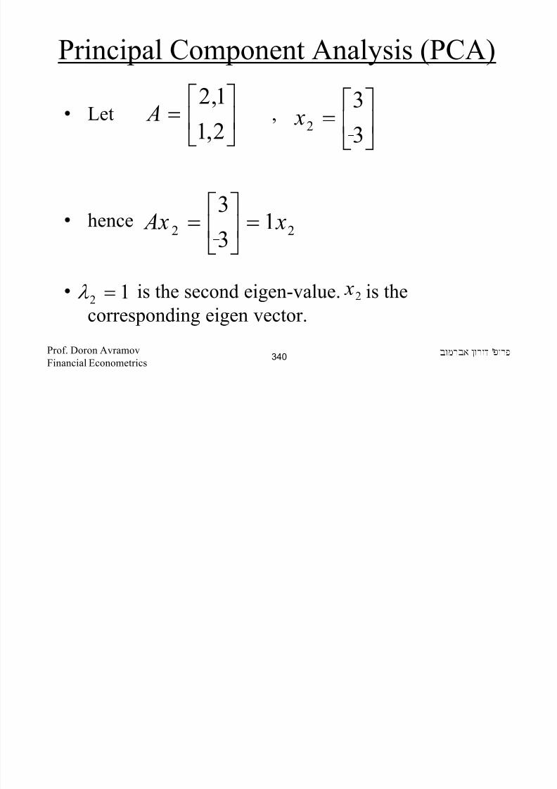
8/22/2019 Avramov Doron Financial Econometrics
http://slidepdf.com/reader/full/avramov-doron-financial-econometrics 340/553
'Prof. Doron Avramov
Financial Econometrics340
Eigen Values and Eigen Vectors• Finding the eigen vector
1,1
32,1
1,2
==
=
y x
y
x
y
x
3,1
12,1
1,2
−==
=
y x
y
x
y
x

8/22/2019 Avramov Doron Financial Econometrics
http://slidepdf.com/reader/full/avramov-doron-financial-econometrics 341/553
'Prof. Doron Avramov
Financial Econometrics341
PCA• You have returns on N stocks for T periods
[ ] R R
T
V
R R R R
let R R R R
R R
N
N N N
T N
T
~'
~1ˆ
~,,
~,
~~
~~
,,
21
111
111
=
=
−=−=
∧∧
××
K
K
K
µ µ

8/22/2019 Avramov Doron Financial Econometrics
http://slidepdf.com/reader/full/avramov-doron-financial-econometrics 342/553
T 'Prof. Doron Avramov
Financial Econometrics342
PCA• Extract K -eigen vectors corresponding to the largest
K -eigen values.• Each of the eigen vector is an N by 1 vector.
• The extraction mechanism is as follows.• The first eigen vector is obtained as
1
'
1 ˆwV w
11
'
1 =ww
1maxw
t s.

8/22/2019 Avramov Doron Financial Econometrics
http://slidepdf.com/reader/full/avramov-doron-financial-econometrics 343/553
'Prof. Doron Avramov
Financial Econometrics343
PCA• is an eigen vector since
• is therefore the highest eigen value.
1w
1'11
111
ˆ
ˆ
wV w
Moreover wwV
=
=
λ
λ
1λ

8/22/2019 Avramov Doron Financial Econometrics
http://slidepdf.com/reader/full/avramov-doron-financial-econometrics 344/553
'Prof. Doron Avramov
Financial Econometrics344
PCA• Extracting the second eigen vector
t s.
2
maxw 2
'
2ˆwV w
0
1
2
'
1
2
'
2
=
=
ww
ww

8/22/2019 Avramov Doron Financial Econometrics
http://slidepdf.com/reader/full/avramov-doron-financial-econometrics 345/553
'Prof. Doron Avramov
Financial Econometrics345
PCA• The optimization yields:
• The second eigen value is smaller than the first due
to the presence of one extra constraint in theoptimization – the orthogonality constraint.
12
'
22
222
ˆ
ˆ
λ λ
λ
<=
=
wV w
wwV

8/22/2019 Avramov Doron Financial Econometrics
http://slidepdf.com/reader/full/avramov-doron-financial-econometrics 346/553
'Prof. Doron Avramov
Financial Econometrics346
PCA• The K -th eigen vector is derived as
t s.
max K K wV w ˆ'
0
0
0
1
1
'
2
'
1
'
'
=
=
=
KK
K
K
K K
ww
ww
ww
ww
M

8/22/2019 Avramov Doron Financial Econometrics
http://slidepdf.com/reader/full/avramov-doron-financial-econometrics 347/553
01 =− K K ww 'Prof. Doron Avramov
Financial Econometrics347
PCA• The optimization yields:
121
' ˆ
ˆ
λ λ λ λ
λ
<<<<=
=
− K K K K K
K K K
wV w
wwV

8/22/2019 Avramov Doron Financial Econometrics
http://slidepdf.com/reader/full/avramov-doron-financial-econometrics 348/553
'Prof. Doron Avramov
Financial Econometrics348
PCA• Then - each of the K-eigen vectors delivers a unique
asset pricing factor.• Simply, multiply excess stock returns by the eigen
vectors:
11
11
11
×××
×××
⋅=
⋅=
N K
N T
e
T K
N N T
e
T
w R F
w R F
M
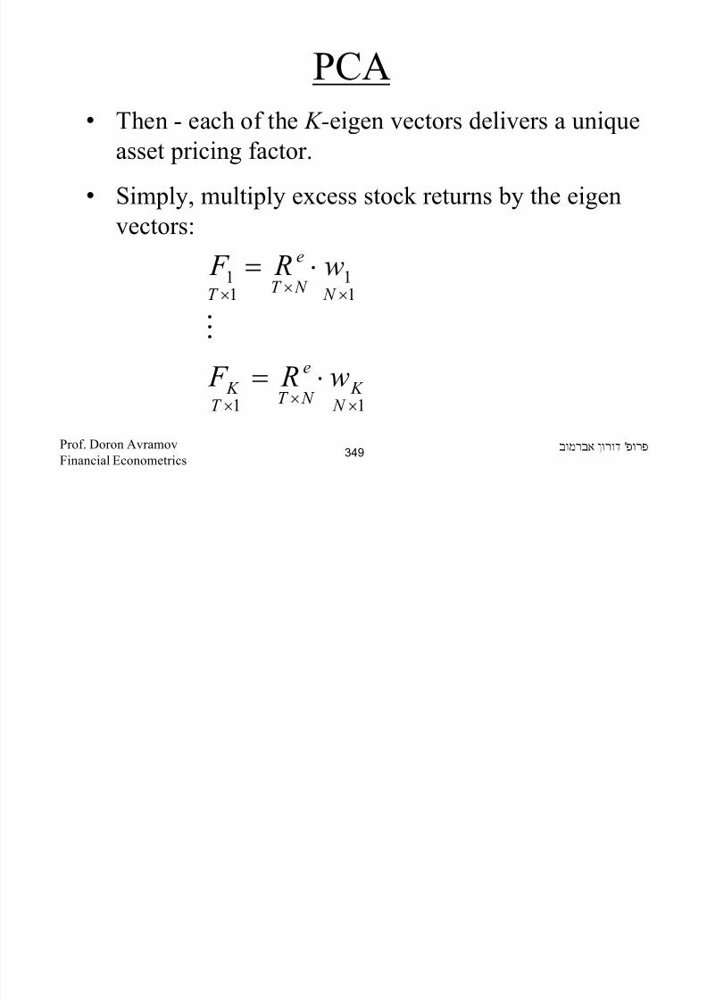
8/22/2019 Avramov Doron Financial Econometrics
http://slidepdf.com/reader/full/avramov-doron-financial-econometrics 349/553
'Prof. Doron Avramov
Financial Econometrics349
PCA• Recall, the basic idea here is to replace the original
set of N variables with a lower dimensional set of K -factors ( K<<N ).
• The contribution of the j-th eigen vector to explain
the covariance matrix of stock returns is
∑=
N
i
i
j
1
λ
λ

8/22/2019 Avramov Doron Financial Econometrics
http://slidepdf.com/reader/full/avramov-doron-financial-econometrics 350/553
'Prof. Doron Avramov
Financial Econometrics350
PCA• Typically the first three eigen vectors explain over
and above 95% of the covariance matrix.
•What does it mean to “explain the covariancematrix”? Coming up soon!
8/22/2019 Avramov Doron Financial Econometrics
http://slidepdf.com/reader/full/avramov-doron-financial-econometrics 351/553
'Prof. Doron Avramov
Financial Econometrics351
Understanding the PCA:Digging Deeper
• The covariance matrix can be decomposed as
[ ]
='
'
,,0
0,
,,ˆ
1,1
1
N
N
w
w
wwV M
K
M
K
K
λ
N λ O
P f D A

8/22/2019 Avramov Doron Financial Econometrics
http://slidepdf.com/reader/full/avramov-doron-financial-econometrics 352/553
'Prof. Doron Avramov
Financial Econometrics352
Understanding the PCA:Digging Deeper
• If some of the are either zero or negative – the covariance matrix is not properly defined -- it is
not positive definite.
• In fixed income analysis – there are three prominent
eigen vectors, or three factors.
• The first factor stands for the term structure level,the second for the term structure slope, and the third
for the curvature of the term structure.
s−λ
P f D A

8/22/2019 Avramov Doron Financial Econometrics
http://slidepdf.com/reader/full/avramov-doron-financial-econometrics 353/553
'Prof. Doron Avramov
Financial Econometrics353
Understanding the PCA:Digging Deeper
• In equity analysis, the first few (up to three)
principal components are prominent.
• Others are around zero.
• The attempt is to replace the sample covariance
matrix by the matrix which mostly summarizes
the information in the sample covariance matrix.
V ~
'Prof Doron Avramov

8/22/2019 Avramov Doron Financial Econometrics
http://slidepdf.com/reader/full/avramov-doron-financial-econometrics 354/553
'Prof. Doron Avramov
Financial Econometrics354
Understanding the PCA:Digging Deeper
• The matrix is given by
• Of course, the dimension of is N by N .
• However, its rank is K , thus the matrix is not
invertible.
[ ]
=×
'
'
,,0
0,
,,
~1,1
1
k
k N N
w
w
wwV MK
M
K
K
λ
k
O
V ~
V ~
'Prof Doron Avramov

8/22/2019 Avramov Doron Financial Econometrics
http://slidepdf.com/reader/full/avramov-doron-financial-econometrics 355/553
invertible.'Prof. Doron Avramov
Financial Econometrics355
• This is the same as asking: what does it mean to
explain the sample covariance matrix?
Is close to ?V
~
V ˆ
'Prof Doron Avramov

8/22/2019 Avramov Doron Financial Econometrics
http://slidepdf.com/reader/full/avramov-doron-financial-econometrics 356/553
'Prof. Doron Avramov
Financial Econometrics356
• Let us represent returns as
M
t Kt K t t t f f f r 1121211111 ε β β β α +++++= K
t r 1~
Nt Kt NK t N t N N Nt f f f r ε β β β α +++++= K2211
Nt r ~
T t ,,1K=∀
T t ,,1K=∀
Is close to ?V
~
V ˆ
'Prof Doron Avramov
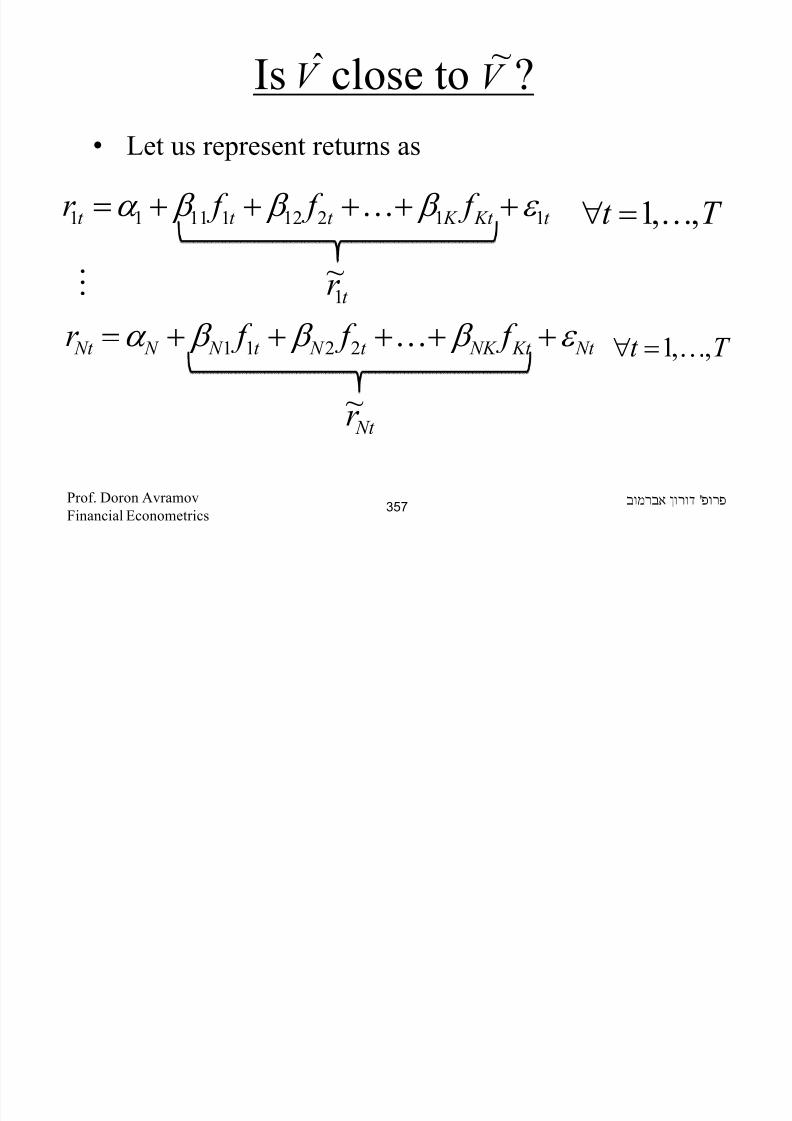
8/22/2019 Avramov Doron Financial Econometrics
http://slidepdf.com/reader/full/avramov-doron-financial-econometrics 357/553
Prof. Doron Avramov
Financial Econometrics357
• where are the principal component based
factors and are the exposures of firm i tothose factors.
Kt t f f K1
iK i β K1
Is close to ?V
~
V ˆ
'Prof. Doron Avramov

8/22/2019 Avramov Doron Financial Econometrics
http://slidepdf.com/reader/full/avramov-doron-financial-econometrics 358/553
Prof. Doron Avramov
Financial Econometrics358
• is closed enough to - if
1. The variances of the residuals cannot be
dramatically reduced by adding more factors.
2. The pairwise cross-section correlations of theresiduals cannot be considerably reduced by
adding more factors.
Is close to ?V
~
V ˆ
V ~
V
'Prof. Doron Avramov359

8/22/2019 Avramov Doron Financial Econometrics
http://slidepdf.com/reader/full/avramov-doron-financial-econometrics 359/553
Financial Econometrics359
The Contribution of the PC-Sto Explain Portfolio Variation
• Let be the exposures of firm i to
the K common factors.
• Let be an N -vector of portfolio weights:
• Recall, R is a T×N matrix of stock returns.
[ ]'
11
,, iK i K
i β β β K=×
pw
[ ] Np p p p wwww ,,, 21 K= '
'Prof. Doron Avramov360

8/22/2019 Avramov Doron Financial Econometrics
http://slidepdf.com/reader/full/avramov-doron-financial-econometrics 360/553
Financial Econometrics360
The Contribution of the PC-Sto Explain Portfolio Variation
• The portfolio’s rate of return is
• Moreover, the portfolio time t return is given by
11 ×××
⋅= N
p
N T T
p w R R
11
'
2211××
⋅≡+++= N
t
N
p Nt Npt pt p pt r wr wr wr w R K
'Prof. Doron Avramov361

8/22/2019 Avramov Doron Financial Econometrics
http://slidepdf.com/reader/full/avramov-doron-financial-econometrics 361/553
Financial Econometrics361
The Contribution of the PC-Sto Explain Portfolio Variation
We can approximate the portfolio’s rate of return as:
( ) Kt K t t p pt f f f w R 12121111
~ β β β +++= K
( )
( ) Kt NK t N t N Np
Kt K t t p
f f f w
f f f w
β β β
β β β
++++
+
++++
K
KKKKKKKKKKKKK
K
2211
22221212
'Prof. Doron Avramov362

8/22/2019 Avramov Doron Financial Econometrics
http://slidepdf.com/reader/full/avramov-doron-financial-econometrics 362/553
Financial Econometrics362
The Contribution of the PC-S
to Explain Portfolio VariationThus,
11
'
12
1
'
2
111
'
1
2211
~
××
××
××
⋅=
⋅=
⋅=
+++=
N
K
N
p K
N N
p
N N p
Kt K t t pt
w
w
w
where f f f R
β δ
β δ
β δ
δ δ δ
M
K
'Prof. Doron Avramov363

8/22/2019 Avramov Doron Financial Econometrics
http://slidepdf.com/reader/full/avramov-doron-financial-econometrics 363/553
Financial Econometrics363
The Contribution of the PC-S
to Explain Portfolio Variation
Notice that
are the K loadings on the common factors,
or they are the risk exposures, while
are the K -realizations of the factors at time t .
K δ δ K1
Kt t f f K1
'Prof. Doron Avramov364

8/22/2019 Avramov Doron Financial Econometrics
http://slidepdf.com/reader/full/avramov-doron-financial-econometrics 364/553
Financial Econometrics364
Explain the Portfolio Variance
• The actual variation is
• The approximated variation is
• Both quantities are quite similar.
p p pt wV w R ˆ)('2
=σ
)var()var()var()~( 2
2
2
21
2
1
2
Kt K t t pt f f f R δ δ δ σ +++= K
'Prof. Doron Avramov
Fi i l E i365

8/22/2019 Avramov Doron Financial Econometrics
http://slidepdf.com/reader/full/avramov-doron-financial-econometrics 365/553
Financial Econometrics365
Explaining the Portfolio
Variance
The contribution of the i-th PC to the overall portfoliosvariance is:
∑=
k
j j j
ii
f
f
1
2
2
)var(
)var(
δ
δ
'Prof. Doron Avramov
Fi i l E t i366

8/22/2019 Avramov Doron Financial Econometrics
http://slidepdf.com/reader/full/avramov-doron-financial-econometrics 366/553
Financial Econometrics
Asy. PCA: What if N>T?• Then create a T×T matrix and extract K eigen
vectors – those eigen vectors are the factors
and is the T -vector of cross sectional (across-stocks) mean of returns.
'ˆ
ˆ'ˆ1ˆ
11 N N
T N T N T R E
where
E E N
V
××
∧
××⋅−=
=
ι µ
µ ˆ
V
'Prof. Doron Avramov
Financial Econometrics367

8/22/2019 Avramov Doron Financial Econometrics
http://slidepdf.com/reader/full/avramov-doron-financial-econometrics 367/553
Financial Econometrics
Other Applications• PCA can be implemented in a host of other
applications.
• For instance, you want to predict economic growth
with many predictors, say M where M is large.
• You have a panel of T×M predictors, where T is the
time-series dimension.
'Prof. Doron Avramov
Financial Econometrics368

8/22/2019 Avramov Doron Financial Econometrics
http://slidepdf.com/reader/full/avramov-doron-financial-econometrics 368/553
Financial Econometrics
Other Applications• In a matrix form
where is the m-the predictor realized at time t .
=×
TM T T
M
M T Z Z Z
Z Z Z
Z
,,,
,,,
21
11211
K
M
K
tm Z
'Prof. Doron Avramov
Financial Econometrics369

8/22/2019 Avramov Doron Financial Econometrics
http://slidepdf.com/reader/full/avramov-doron-financial-econometrics 369/553
Financial Econometrics
Other Applications• If T>M compute the covariance matrix of Z – then
extract K principal components such that yousummarize the M -dimension of the predictors with a
smaller subspace of order K<<M.
• You extract eigen vectors.
11
1 ,,
×× M
K
M
ww K
'Prof. Doron Avramov
Financial Econometrics370

8/22/2019 Avramov Doron Financial Econometrics
http://slidepdf.com/reader/full/avramov-doron-financial-econometrics 370/553
Financial Econometrics
Other Applications• Then you construct K predictors:
11
11
11
×××
×××
⋅=
⋅=
M K
M T T K
M M T T
w Z Z
w Z Z
M
'Prof. Doron Avramov
Financial Econometrics371

8/22/2019 Avramov Doron Financial Econometrics
http://slidepdf.com/reader/full/avramov-doron-financial-econometrics 371/553
Financial Econometrics
What if M>T ?• If M>T then you extract K eigen vectors from the
T×T matrix.
• In this case, the K -predictors are the extracted K eigen vectors.
• Be careful of a look-ahead bias in real time
prediction.
'Prof. Doron Avramov
Financial Econometrics372

8/22/2019 Avramov Doron Financial Econometrics
http://slidepdf.com/reader/full/avramov-doron-financial-econometrics 372/553
The Number of Factors in PCA• An open question is: how many factors/eigen vectors
should be extracted?
• Here is a good mechanism: set - the highest
number of factors.
• Run the following multivariate regression for
'Prof. Doron Avramov
Financial Econometrics373
max K
max,,2,1 K K K=
N T N K K T N T N T E F R
×××××× +++= ''11
β α ι
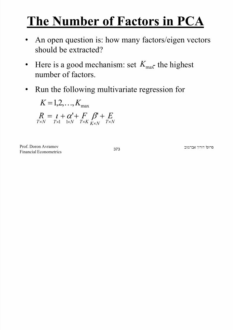
8/22/2019 Avramov Doron Financial Econometrics
http://slidepdf.com/reader/full/avramov-doron-financial-econometrics 373/553
The Number of Factors in PCA• Estimate first the residual covariance matrix and then
the average of residual variances:
• Where is the sum of diagonal elements in
'Prof. Doron Avramov
Financial Econometrics374
( ) ( ) N
V tr K
E E K T
V N N
ˆˆ
ˆ'ˆ1
1ˆ
2 =
−−=
×
σ
V tr ˆ V ˆ

8/22/2019 Avramov Doron Financial Econometrics
http://slidepdf.com/reader/full/avramov-doron-financial-econometrics 374/553
The Number of Factors in PCA
Compute for each chosen K
and pick K which minimizes this criterion.
'Prof. Doron Avramov
Financial Econometrics375
( ) ( ) ( )
+
⋅+
+=T N
NT
NT
T N K K K K PC lnˆˆ
max
22 σ σ

8/22/2019 Avramov Doron Financial Econometrics
http://slidepdf.com/reader/full/avramov-doron-financial-econometrics 375/553
Lecture Notes inFinancial Econometrics
The Black-Litterman (BL) Approach
for Estimating Mean Returns:Basics, Extensions, and
Incorporating Market Anomalies
'Prof. Doron Avramov
Financial Econometrics376

8/22/2019 Avramov Doron Financial Econometrics
http://slidepdf.com/reader/full/avramov-doron-financial-econometrics 376/553
Estimating Mean Returns – The Bayesian Perspective
• Thus far, we have been dealing with classical, also termedfrequentist, econometrics.
• Indeed, GMM, MLE, etc. are all classical methods.
• The competing perspective is the Bayesian.• The BL approach is Bayesian.
• Theoretically, the Bayesian approach is the most appealing
for decision making, such as asset allocation, securityselection, and policy making in general.
• Major advantages: accounting for estimation risk, model
risk, informative priors, and it is numerically tractable.
'Prof. Doron Avramov
Financial Econometrics377
8/22/2019 Avramov Doron Financial Econometrics
http://slidepdf.com/reader/full/avramov-doron-financial-econometrics 377/553
Estimating Mean Returns –
The Bayesian Perspective
• To explain the difference between classical and Bayesian
methods, assume that you observe the market returns over T
periods:
• The classical approach computes the sample mean return,
which is a stochastic (random) variable, and then specifies a
distribution for the mean return.
mT mm R R R ,,, 21 K
'Prof. Doron Avramov
Financial Econometrics378

8/22/2019 Avramov Doron Financial Econometrics
http://slidepdf.com/reader/full/avramov-doron-financial-econometrics 378/553
Estimating Mean Returns –
The Bayesian Perspective
• For instance, assume that
• Then the sample mean is distributed as
2,~ mmt N R σ µ
'Prof. Doron Avramov
Financial Econometrics379
T N r m
2
,~σ
µ

8/22/2019 Avramov Doron Financial Econometrics
http://slidepdf.com/reader/full/avramov-doron-financial-econometrics 379/553
Estimating Mean Returns –
The Bayesian Perspective
•The Bayesian approach is very different – the unobserved
actual mean return is the stochastic variable.
•The econometrician specifies both prior as well as likelihood
(data based) distributions for the mean return:
Prior: Likelihood:2,~ p p N σ µ µ 2,~ L L N σ µ µ
'Prof. Doron Avramov
Financial Econometrics380

8/22/2019 Avramov Doron Financial Econometrics
http://slidepdf.com/reader/full/avramov-doron-financial-econometrics 380/553
Estimating Mean Returns –
The Posterior Distribution
• The inference is then based on the posterior distributionwhich combines the prior and the likelihood.
• In particular, given the above specified prior and likelihood based distributions, the posterior density is given by
2~
,
~
~ σ µ µ N
'Prof. Doron Avramov
Financial Econometrics381

8/22/2019 Avramov Doron Financial Econometrics
http://slidepdf.com/reader/full/avramov-doron-financial-econometrics 381/553
Estimating Mean Returns –
The Posterior Distribution
The mean and variance of the posterior are
( L p ww µ µ µ 11 1~ −+=
1
22
2 11~−
+=
L p σ σ σ
'Prof. Doron Avramov
Financial Econometrics382

8/22/2019 Avramov Doron Financial Econometrics
http://slidepdf.com/reader/full/avramov-doron-financial-econometrics 382/553
The Posterior Mean Return• The posterior mean return is a weighted average of the prior
mean and the sample mean with weights proportional to the
precision of the prior versus the sample means, where
precision defined as the reciprocal of the variance.
• In particular,
22
2
1 11
1
L p
pw
σ σ
σ
+=
22
2
12 11
1
1
L p
Lww
σ σ
σ
+=−=;
'Prof. Doron Avramov
Financial Econometrics383

8/22/2019 Avramov Doron Financial Econometrics
http://slidepdf.com/reader/full/avramov-doron-financial-econometrics 383/553
Estimating Mean Returns• It is notoriously difficult to propose good estimates for
mean returns.
• The sample means are quite noisy – thus asset pricing
models -even if misspecified -could give a good guidance.
• To illustrate, you consider a K -factor model (factors are portfolio spreads) and you run the time series regression
112
121
1111 ×××××× +++++= N
t Kt N
K t N
t N N N
e
t e f f f r β β β α K
'Prof. Doron Avramov
Financial Econometrics384

8/22/2019 Avramov Doron Financial Econometrics
http://slidepdf.com/reader/full/avramov-doron-financial-econometrics 384/553
Estimating Mean Returns• Then the estimated excess mean return is given by
where are the sample estimates of factor
loadings, and are the sample estimates of the
factor mean returns.
K f K f f
e µ β µ β µ β µ ˆˆˆˆˆˆˆ21 21 +++= K
K β β β ˆˆ,ˆ 21 K
K f f f µ µ µ ˆˆ,ˆ21K
'Prof. Doron Avramov
Financial Econometrics385

8/22/2019 Avramov Doron Financial Econometrics
http://slidepdf.com/reader/full/avramov-doron-financial-econometrics 385/553
The BL Mean Returns• The BL approach combines a model (CAPM) with some
views, either relative or absolute, about expected returns.
• The BL vector of mean returns is given by
Ω+
∑⋅
Ω+
∑=
××
−
××
−
××
−
××
−
×
−
××× 1
1
1
1
11
1
11
111
'' K
v
K K K N N
eq
N N N K K K K N N N N BL P P P µ µ τ τ µ
'Prof. Doron Avramov
Financial Econometrics386

8/22/2019 Avramov Doron Financial Econometrics
http://slidepdf.com/reader/full/avramov-doron-financial-econometrics 386/553
Understanding the BL Formulation
• We need to understand the essence of the following
parameters, which characterize the mean return vector
• Starting from the matrix – you can choose any of the
specifications derived in the previous meetings – either the
sample covariance matrix, or the equal correlation, or an
asset pricing based covariance, or you could rely on the LWshrinkage approach – either the complex or the naïve one.
veq P µ τ µ ,,,,, Ω∑
Σ
'Prof. Doron Avramov
Financial Econometrics387

8/22/2019 Avramov Doron Financial Econometrics
http://slidepdf.com/reader/full/avramov-doron-financial-econometrics 387/553
Constructing Equilibrium
Expected Returns• The , which is the equilibrium vector of expected
return, is constructed as follows.
• Generate , the N ×1 vector denoting the weights of
any of the N securities in the market portfolio based on
market capitalization. Of course, the sum of weights must be unity.
• Then, the price of risk is where and
are the expected return and variance of the market portfolio.
• Later, we will justify this choice for the price of risk.
eqµ
MKT ω
2
m
m Rf
σ
µ γ
−= 2
mσ m
µ
'Prof. Doron Avramov
Financial Econometrics388

8/22/2019 Avramov Doron Financial Econometrics
http://slidepdf.com/reader/full/avramov-doron-financial-econometrics 388/553
Constructing EquilibriumExpected Returns
• One could pick a range of values for going from 1.5 to2.5 and examine performance of each choice.
• If you work with monthly observations, then switching to the
annual frequency does not change as both the numerator
and denominator are multiplied by 12.
• Having at hand both and , the equilibrium return
vector is given by
γ
γ
MKT ω γ
MKT
eq ω γ µ Σ=
'Prof. Doron Avramov
Financial Econometrics389

8/22/2019 Avramov Doron Financial Econometrics
http://slidepdf.com/reader/full/avramov-doron-financial-econometrics 389/553
Constructing EquilibriumExpected Returns
• This vector is called neutral mean or equilibrium expectedreturn.
• To understand why, notice that if you have a utility function
that generates the tangency portfolio of the form
then using as the vector of excess returns on the N assets
would deliver as the tangency portfolio.
e
e
TP wµ ι
µ 1
1
' −
−
∑∑
=
eqµ
MKT ω
'Prof. Doron Avramov
Financial Econometrics390

8/22/2019 Avramov Doron Financial Econometrics
http://slidepdf.com/reader/full/avramov-doron-financial-econometrics 390/553
What if you Directly Applythe CAPM?
• The question being – would you get the same vector of
equilibrium mean return if you directly use the CAPM?
• Yes, if…
'Prof. Doron Avramov
Financial Econometrics391

8/22/2019 Avramov Doron Financial Econometrics
http://slidepdf.com/reader/full/avramov-doron-financial-econometrics 391/553
The CAPM based Expected
Returns• Under the CAPM the vector of excess returns is given by
( ) ( )( )
MKT
e
m
m
MKT
N
e
m
MKT
m
MKT
ee
m
e
m
e
e
m N N
e
ww
CAPM
wwr r r r
∑=∑
=
∑===
=
×
××
γ µ σ
µ
σ σ σ β
µ β µ
21
222
11
:
',cov,cov
'Prof. Doron Avramov
Financial Econometrics392

8/22/2019 Avramov Doron Financial Econometrics
http://slidepdf.com/reader/full/avramov-doron-financial-econometrics 392/553
What if you use Directly the
CAPM?
Since and
then
( ) MKT ee
m w'µ µ = ( ) MKT ee
m wr r '=
eq MKT
m
e
me w µ σ µ µ =∑= 2
'Prof. Doron Avramov
Financial Econometrics393
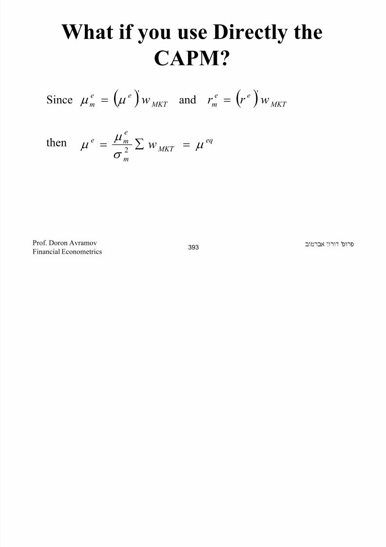
8/22/2019 Avramov Doron Financial Econometrics
http://slidepdf.com/reader/full/avramov-doron-financial-econometrics 393/553
What if you use Directly theCAPM?
• So indeed, if you use (i) the sample covariance matrix, rather than any other specification, as well as (ii)
then the BL equilibrium expected returns and expected
returns based on the CAPM are identical.
2
m
m Rf
σ
µ
γ
−=
'Prof. Doron Avramov
Financial Econometrics394

8/22/2019 Avramov Doron Financial Econometrics
http://slidepdf.com/reader/full/avramov-doron-financial-econometrics 394/553
The P Matrix: Absolute Views• In the BL approach the investor/econometrician forms some
views about expected returns as described below.
• P is defined as that matrix which identifies the assets
involved in the views.
• To illustrate, consider two "absolute" views only.
• The first view says that stock 3 has an expected return of 5%
while the second says that stock 5 will deliver 12%.
'Prof. Doron Avramov
Financial Econometrics395

8/22/2019 Avramov Doron Financial Econometrics
http://slidepdf.com/reader/full/avramov-doron-financial-econometrics 395/553
The P Matrix: Absolute Views• In general the number of views is K .
• In our case K=2.
• Then P is a 2 ×N matrix.
• The first row is all zero except for the fifth entry which is
one.
• Likewise, the second row is all zero except for the fifth entry
which is one.
'Prof. Doron Avramov
Financial Econometrics396

8/22/2019 Avramov Doron Financial Econometrics
http://slidepdf.com/reader/full/avramov-doron-financial-econometrics 396/553
The P Matrix: Relative Views• Let us consider now two "relative views".
• Here we could incorporate market anomalies into the BL paradigm.
• Market anomalies are cross sectional patterns in stock
returns unexplained by the CAPM.
• Example: price momentum, earnings momentum, value, size,
accruals, credit risk, dispersion, and volatility.
'Prof. Doron Avramov
Financial Econometrics397

8/22/2019 Avramov Doron Financial Econometrics
http://slidepdf.com/reader/full/avramov-doron-financial-econometrics 397/553
Black-Litterman: Momentum and
Value Effects
• Let us focus on price momentum and the value effects.
• Assume that both momentum and value investing outperform.
• The first row of P corresponds to momentum investing.• The second row corresponds to value investing.
• Both the first and second rows contain N elements.
'Prof. Doron Avramov
Financial Econometrics398

8/22/2019 Avramov Doron Financial Econometrics
http://slidepdf.com/reader/full/avramov-doron-financial-econometrics 398/553
Winner, Loser, Value, and
Growth Stocks
•Winner stocks are the top 10% performers during the past sixmonths.
•Loser stocks are the bottom 10% performers during the past six
months.
•Value stocks are 10% of the stocks having the highest book-to-
market ratio.
•Growth stocks are 10% of the stocks having the lowest book-
to-market ratios.
'Prof. Doron Avramov
Financial Econometrics399

8/22/2019 Avramov Doron Financial Econometrics
http://slidepdf.com/reader/full/avramov-doron-financial-econometrics 399/553
Momentum and Value Payoffs
• The momentum payoff is a return spread – return on anequal weighted portfolio of winner stocks minus return on
equal weighted portfolio of loser stocks.
• The value payoff is also a return spread – the returndifferential between equal weighted portfolios of value and
growth stocks.
'Prof. Doron Avramov
Financial Econometrics400

8/22/2019 Avramov Doron Financial Econometrics
http://slidepdf.com/reader/full/avramov-doron-financial-econometrics 400/553
Back to the P Matrix
• Suppose that the investment universe consists of 100 stocks
• The first row gets the value 0.1 if the corresponding stock is a
winner (there are 10 winners in a universe of 100 stocks).
• It gets the value -0.1 if the corresponding stock is a loser (there
are 10 losers).
• Otherwise it gets the value zero.
• The same idea applies to value investing.
• Of course, since we have relative views here (e.g., return on
winners minus return on losers) then the sums of the first row
and the sum of the second row are both zero.
'Prof. Doron Avramov
Financial Econometrics401

8/22/2019 Avramov Doron Financial Econometrics
http://slidepdf.com/reader/full/avramov-doron-financial-econometrics 401/553
Back to the P Matrix• More generally, if N stocks establish the investment universe
and moreover momentum and value are based on deciles (thereturn difference between the top and bottom deciles) then
the winner stock is getting 10/N
while the loser stock gets -10/N .
• The same applies to value versus growth stocks.
• Rule: the sum of the row corresponding to absolute views is
one, while the sum of the row corresponding to relative
views is zero.
'Prof. Doron Avramov
Financial Econometrics402

8/22/2019 Avramov Doron Financial Econometrics
http://slidepdf.com/reader/full/avramov-doron-financial-econometrics 402/553
Computing the Vector
• It is the K ×1 vector of K views on expected returns.
• Using the absolute views above
• Using the relative views above, the first element is the
payoff to momentum trading strategy (sample mean); the
second element is the payoff to value investing (samplemean).
vµ
[ ]'0.05,0.12=vµ
'Prof. Doron Avramov
Financial Econometrics403

8/22/2019 Avramov Doron Financial Econometrics
http://slidepdf.com/reader/full/avramov-doron-financial-econometrics 403/553
The Matrix
• is a K ×K covariance matrix expressing uncertainty
about views.
• It is typically assumed to be diagonal.
• In the absolute views case described above denotes
uncertainty about the first view while denotes
uncertainty about the second view – both are at thediscretion of the econometrician/investor.
ΩΩ
( )1,1Ω( )2,2Ω
'Prof. Doron Avramov
Financial Econometrics404

8/22/2019 Avramov Doron Financial Econometrics
http://slidepdf.com/reader/full/avramov-doron-financial-econometrics 404/553
The Matrix
• In the relative views described above: denotes
uncertainty about momentum. This could be the sample
variance of the momentum payoff.
• denotes uncertainty about the value payoff. This is thecould be the sample variance of the value payoff.
Ω
( )1,1Ω
( )2,2Ω
'Prof. Doron Avramov
Financial Econometrics405

8/22/2019 Avramov Doron Financial Econometrics
http://slidepdf.com/reader/full/avramov-doron-financial-econometrics 405/553
Deciding Upon
• There are many debates among professionals about the right
value of .• From a conceptual perspective it should be 1/T where T
denotes the sample size.
• You can pick
• You can also use other values and examine how they
perform in real-time investment decisions.
τ
τ
1.0=τ
'Prof. Doron Avramov
Financial Econometrics406

8/22/2019 Avramov Doron Financial Econometrics
http://slidepdf.com/reader/full/avramov-doron-financial-econometrics 406/553
Maximizing Sharpe Ratio
• The remaining task is to run the maximization program
• such that each of the w elements is bounded below by 0 and
subject to some agreed upon upper bound, as well as the sum
of the w elements is equal to one.
ww
w BLw
Σ''
maxµ
'Prof. Doron Avramov
Financial Econometrics407

8/22/2019 Avramov Doron Financial Econometrics
http://slidepdf.com/reader/full/avramov-doron-financial-econometrics 407/553
Extending the BL Model to Incorporate Sample
Moments
• Consider a sample of size T , e.g., T=60 monthly
observations.
• Let us estimate the mean and covariance (V ) of our N assets
based on the sample.
• Then the vector of expected return that serves as an input for
asset allocation is given by
where[ ] [ ] sample sample BL sample T V T V µ µ µ
11111
)/()/(−−−−−
+∆+∆=
[ ] 111 ')(−−− Ω+Σ=∆ P P τ
'Prof. Doron Avramov
Financial Econometrics408

8/22/2019 Avramov Doron Financial Econometrics
http://slidepdf.com/reader/full/avramov-doron-financial-econometrics 408/553
Class Notes in
Financial Econometrics
Risk Management:Down Side Risk Measures
'Prof. Doron Avramov
Financial Econometrics409

8/22/2019 Avramov Doron Financial Econometrics
http://slidepdf.com/reader/full/avramov-doron-financial-econometrics 409/553
Downside Risk
•Downside risk is the financial risk associatedwith losses.
• Downside risk measures quantify the risk of
losses, whereas volatility measures are bothabout the upside and downside outcomes.
• That is, volatility treats symmetrically up and
down moves (relative to the mean).• Or volatility is about the entire distribution while
down side risk concentrates on the left tail.'Prof. Doron Avramov
Financial Econometrics410

8/22/2019 Avramov Doron Financial Econometrics
http://slidepdf.com/reader/full/avramov-doron-financial-econometrics 410/553
Downside Risk
• Example of downside risk measures
• Value at Risk (VaR)
• Expected Shortfall
• Semi-variance
• Maximum drawdown• Downside Beta
• Shortfall probability
• We will discuss below all these measures.
'Prof. Doron Avramov
Financial Econometrics411

8/22/2019 Avramov Doron Financial Econometrics
http://slidepdf.com/reader/full/avramov-doron-financial-econometrics 411/553
Value at Risk (VaR)• The says that there is a 5% chance that the
realized return, denoted by R, will be less than .
• More generally,
%95VaR
%95VaR−
µ %95VaR−
( ) α α =−≤ −1Pr VaR R
%5
'Prof. Doron Avramov
Financial Econometrics412

8/22/2019 Avramov Doron Financial Econometrics
http://slidepdf.com/reader/full/avramov-doron-financial-econometrics 412/553
Value at Risk (VaR )( ) ( )( )α σ µ α
σ
µ α
α 1
1
11 −−
−− Φ+−=⇒Φ=−−
VaRVaR
where
, the critical value, is the inverse cumulative
distribution function of the standard normal evaluated at α.
• Let α=5% and assume that
• The critical value is
( )α 1−Φ
( )2
,~ σ µ N R
( ) 64.105.01 −=Φ −
'Prof. Doron Avramov
Financial Econometrics413

8/22/2019 Avramov Doron Financial Econometrics
http://slidepdf.com/reader/full/avramov-doron-financial-econometrics 413/553
Therefore
Value at Risk (VaR)
Check:
If
Then
( 2,~ σ µ N R
( )
( ) ( ) 05.064.164.1Pr
64.1Pr
Pr Pr 1
=−Φ=−<=
−−<−=
−−≤
−=−≤ −
z
R
VaR RVaR R
σ µ σ µ
σ µ
σ
µ
σ
µ α α
( )( ) σ µ σ α µ α 64.11
1 +−=Φ+−= −−VaR
'Prof. Doron Avramov
Financial Econometrics414

8/22/2019 Avramov Doron Financial Econometrics
http://slidepdf.com/reader/full/avramov-doron-financial-econometrics 414/553
Example: The US Equity Premium
• Suppose:
• That is to say that we are 95% sure that the future equity
premium won’t decline more than 25%.• If we would like to be 97.5% sure – the price is that the
threshold loss is higher.
• To illustrate,
( )( ) 25.020.064.108.0
20.0,08.0~
95.0
2
=⋅−−=⇒ VaR
N R
( ) 31.020.096.108.0975.0 =⋅−−=VaR
'Prof. Doron Avramov
Financial Econometrics415

8/22/2019 Avramov Doron Financial Econometrics
http://slidepdf.com/reader/full/avramov-doron-financial-econometrics 415/553
VaR of a Portfolio• Evidently, the VaR of a portfolio is not necessarily lower
than the combination of individual VaR-s – which is
apparently at odds with the notion of diversification.
• However, recall that VaR is a downside risk measure while
volatility which diminishes at the portfolio level is a
symmetric measure.
'Prof. Doron Avramov
Financial Econometrics416
8/22/2019 Avramov Doron Financial Econometrics
http://slidepdf.com/reader/full/avramov-doron-financial-econometrics 416/553
Backtesting the VaR • The VaR requires the specification of the exact distribution
and its parameters (e.g., mean and variance).
• Typically the normal distribution is chosen.
• Mean could be the sample average.
• Volatility estimates could follow ARCH, GARCH,
EGARCH, stochastic volatility, and realized volatility, all
of which are described later in this course.
• We can examine the validity of VaR using backtesting.'Prof. Doron Avramov
Financial Econometrics417

8/22/2019 Avramov Doron Financial Econometrics
http://slidepdf.com/reader/full/avramov-doron-financial-econometrics 417/553
Backtesting the VaR • Assume that stock returns are normally distributed with
mean and variance that vary over time
• The sample is of length T .
• Receipt for backtesting is as follows.
• Use the first, say, sixty monthly observations to estimate
the mean and volatility and compute the VaR.• If the return in month 61 is below the VaR set an indicator
function I to be equal to one; otherwise, it is zero.
T t ,,2,1 K=∀2,~ t t t N r σ µ
'Prof. Doron AvramovFinancial Econometrics
418

8/22/2019 Avramov Doron Financial Econometrics
http://slidepdf.com/reader/full/avramov-doron-financial-econometrics 418/553
Backtesting the VaR • Repeat this process using either a rolling or recursive
schemes and compute the fraction of time when the next
period return is below the VaR.
• If α=5% - only 5% of the returns should be below the
computed VaR.
• Suppose we get 5.5% of the time – is it a bad model or just
a bad luck?
'Prof. Doron AvramovFinancial Econometrics
419
8/22/2019 Avramov Doron Financial Econometrics
http://slidepdf.com/reader/full/avramov-doron-financial-econometrics 419/553
Model Verification Based on
Failure Rates• To answer that question – let us discuss another example
which requires a similar test statistic.
• Suppose that Y analysts are making predictions about the
market direction for the upcoming year. The analysts
forecast whether market is going to be up or down.
• After the year passes you count the number of wrong
analysts. An analyst is wrong if he/she predicts up movewhen the market is down, or predict down move when the
market is up.
'Prof. Doron AvramovFinancial Econometrics
420

8/22/2019 Avramov Doron Financial Econometrics
http://slidepdf.com/reader/full/avramov-doron-financial-econometrics 420/553
Model Verification Based onFailure Rates
• Suppose that the number of wrong analysts is x.
• Thus, the fraction of wrong analysts is P=x/Y – this is thefailure rate.
'Prof. Doron AvramovFinancial Econometrics
421

8/22/2019 Avramov Doron Financial Econometrics
http://slidepdf.com/reader/full/avramov-doron-financial-econometrics 421/553
The Test Statistic
• The hypothesis to be tested is
• Under the null hypothesis it follows that
Otherwise H
P P H
:
:
1
00 =
( ) ( ) x y x P P x y x f
−−
= 00 1
'Prof. Doron AvramovFinancial Econometrics
422

8/22/2019 Avramov Doron Financial Econometrics
http://slidepdf.com/reader/full/avramov-doron-financial-econometrics 422/553
The Test Statistic
• Notice that
( )
( ) ( )
( )( )1,0~
1
1
00
0
00
0
N y P P
y P x Z
Thus
y P P xVaR
y P x E
−
−=
−=
=
'Prof. Doron AvramovFinancial Econometrics
423
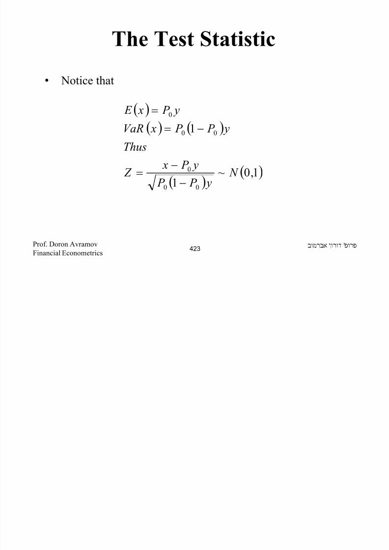
8/22/2019 Avramov Doron Financial Econometrics
http://slidepdf.com/reader/full/avramov-doron-financial-econometrics 423/553
Back to Backtesting VaR: A
Real Life Example
• In its 1998 annual report, JP Morgan explains: In 1998,daily revenue fell short of the downside (95%VaR) band
on 20 trading days (out of 252) or more than 5% of the
time (252×5%=12.6).
• Is the difference just a bad luck or something more
systematic? We can test the hypothesis that it is a bad luck.
Otherwise H
x H
:
6.12:
1
0 =14.2
25295.005.0
6.1220=
⋅⋅
−= Z
'Prof. Doron AvramovFinancial Econometrics
424

8/22/2019 Avramov Doron Financial Econometrics
http://slidepdf.com/reader/full/avramov-doron-financial-econometrics 424/553
Back to Backtesting VaR: A
Real Life Example
• Notice that you reject the null since 2.14 is higher than the
critical value of 1.96.
• That suggests that JPM should search for a better model.• They did find out that the problem was that the actual
revenue departed from the normal distribution.
'Prof. Doron AvramovFinancial Econometrics
425

8/22/2019 Avramov Doron Financial Econometrics
http://slidepdf.com/reader/full/avramov-doron-financial-econometrics 425/553
Expected Shortfall (ES): Truncated
Distribution
• ES is the expected value of the loss conditional upon the
event that the actual return is below the VaR.
• The ES is formulated as
[ ]α α −− −≤−= 11 | VaR R R E ES
'Prof. Doron AvramovFinancial Econometrics
426

8/22/2019 Avramov Doron Financial Econometrics
http://slidepdf.com/reader/full/avramov-doron-financial-econometrics 426/553
Expected Shortfall (ES) and the
Truncated Normal Distribution
• Assume that returns are normally distributed:
( 2,~ σ µ N R
( )( )( )
α
α φ σ µ
σ α µ
α
α
1
1
1
1 |−
−
−−
Φ+−=⇒
Φ+≤−=⇒
ES
R R E ES
'Prof. Doron AvramovFinancial Econometrics
427
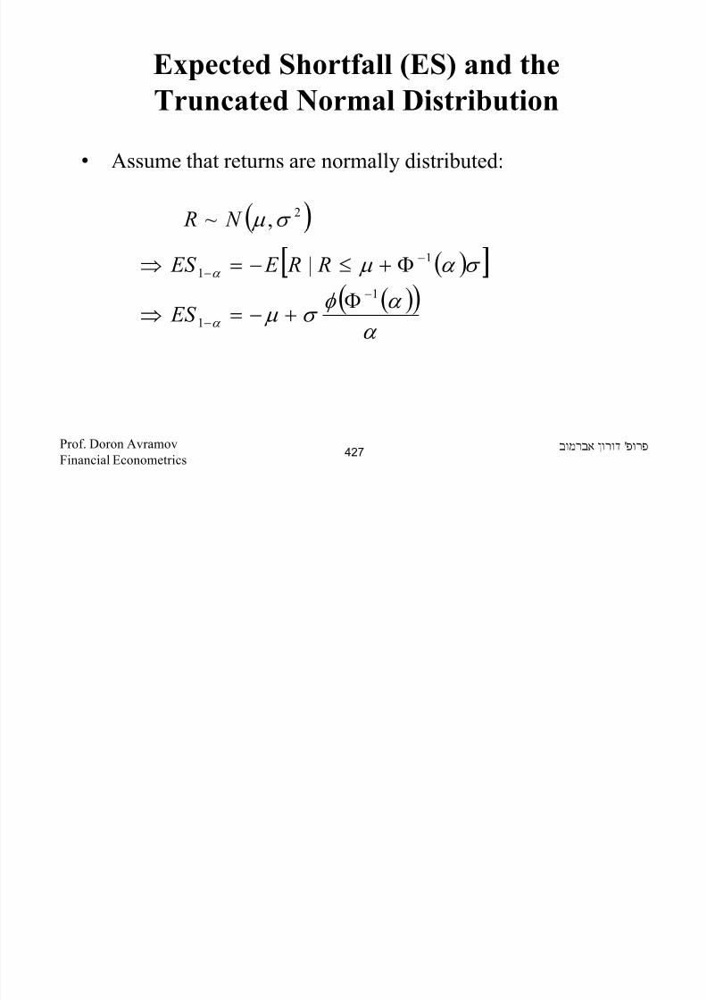
8/22/2019 Avramov Doron Financial Econometrics
http://slidepdf.com/reader/full/avramov-doron-financial-econometrics 427/553
Expected Shortfall (ES) and the
Truncated Normal Distribution
where is the pdf of the standard normal density
e.g
This formula for ES is about the expected value of a
truncated normally distributed random variable.
( )⋅φ
( ) 0.10396164.1 =−φ
'Prof. Doron AvramovFinancial Econometrics
428

8/22/2019 Avramov Doron Financial Econometrics
http://slidepdf.com/reader/full/avramov-doron-financial-econometrics 428/553
Expected Shortfall (ES) and the
Truncated Normal Distribution
Proof:
since
( )
( )( )( )
( )( )α
α φ σ µ κ
κ σφ µ
σ µ
α
1
0
01
2
|
,~
−
−
Φ−=Φ−=−≤ VaR x x E
N x
( )α σ
µ
κ α 11
0
−−
Φ=−−
=VaR
'Prof. Doron AvramovFinancial Econometrics
429

8/22/2019 Avramov Doron Financial Econometrics
http://slidepdf.com/reader/full/avramov-doron-financial-econometrics 429/553
Expected Shortfall: Example
Example
( )
( ) 40.025.0
06.020.008.0
025.0
96.120.008.0
32.005.0
10.020.008.0
05.0
64.120.008.0
%20
%8
%5.97
%95
=+−≈−+−=
=+−≈−
+−=
=
=
φ
φ
σ
µ
ES
ES
'Prof. Doron AvramovFinancial Econometrics
430

8/22/2019 Avramov Doron Financial Econometrics
http://slidepdf.com/reader/full/avramov-doron-financial-econometrics 430/553
Expected Shortfall (ES) and the
Truncated Normal Distribution
• Previously, we got that the VaRs corresponding to those parameters are 25% and 31%.
• Now the expected losses are higher, 32% and 40%.
• Why?• The first lower figures (VaR) are unconditional in nature
relying on the entire distribution.
• In contrast, the higher ES figures are conditional on the
existence of shortfall – realized return is below the VaR.
'Prof. Doron AvramovFinancial Econometrics
431

8/22/2019 Avramov Doron Financial Econometrics
http://slidepdf.com/reader/full/avramov-doron-financial-econometrics 431/553
Expected Shortfall in
Decision Making
• The mean variance paradigm minimizes portfolio volatility
subject to an expected return target.
• Suppose you attempt to minimize ES instead subject toexpected return target.
'Prof. Doron AvramovFinancial Econometrics
432

8/22/2019 Avramov Doron Financial Econometrics
http://slidepdf.com/reader/full/avramov-doron-financial-econometrics 432/553
Expected Shortfall with
Normal Returns
• If stock returns are normally distributed then the ES chosen
portfolio would be identical to that based on the mean
variance paradigm.• No need to go through optimization to prove that assertion.
• Just look at the expression for ES under normality to
quickly realize that you need to minimize the volatility of
the portfolio subject to an expected return target.
'Prof. Doron AvramovFinancial Econometrics
433

8/22/2019 Avramov Doron Financial Econometrics
http://slidepdf.com/reader/full/avramov-doron-financial-econometrics 433/553
Target Semi Variance
• Variance treats equally downside risk and upside potential.
• The semi-variance, just like the VaR, looks at the downside.
• The target semi-variance is defined as:
where h is some target level.
• For instance,
• Unlike the variance,
f Rh =
( ) ( )[ ]20,min hr E h −=λ
( )22 µ σ −= r E
'Prof. Doron AvramovFinancial Econometrics
434

8/22/2019 Avramov Doron Financial Econometrics
http://slidepdf.com/reader/full/avramov-doron-financial-econometrics 434/553
Target Semi Variance
• The target semi-variance:
I. Picks a target level as a reference point instead of the
mean.
II. Gives weight only to negative deviations from a
reference point.
'Prof. Doron AvramovFinancial Econometrics
435
T t S i V i

8/22/2019 Avramov Doron Financial Econometrics
http://slidepdf.com/reader/full/avramov-doron-financial-econometrics 435/553
Target Semi Variance
• Notice that if
where
and are the PDF and CDF of a variable,
respectively
• Of course if
then
( 2,~ σ µ N r
( )
−Φ
+
−+
−−= σ
µ
σ
µ
σ σ
µ
φ σ
µ
σ λ
hhhh
h 1
2
22
Φφ ( )1,0 N
µ =h
( )2
2σ λ =h
'Prof. Doron AvramovFinancial Econometrics
436

8/22/2019 Avramov Doron Financial Econometrics
http://slidepdf.com/reader/full/avramov-doron-financial-econometrics 436/553
Maximum Drawdown (MD)
• The MD (M) over a given investment horizon is the largest
M-month loss of all possible M-month continuous periods
over the entire horizon.
• Useful for an investor who does not know the entry/exit
point and is concerned about the worst outcome.
• It helps determine the investment risk.
'Prof. Doron AvramovFinancial Econometrics
437

8/22/2019 Avramov Doron Financial Econometrics
http://slidepdf.com/reader/full/avramov-doron-financial-econometrics 437/553
Down Size Beta
• I will introduce three distinct measures of downsize beta –
each of which is valid and captures the down side of
investment payoffs.
• Displayed are the population betas.
• Taking the formulations into the sample – simply replace the
expected value by the sample mean.
'Prof. Doron AvramovFinancial Econometrics
438

8/22/2019 Avramov Doron Financial Econometrics
http://slidepdf.com/reader/full/avramov-doron-financial-econometrics 438/553
Downside Beta
• The numerator in the equation is referred to as the co-semi-
variance of returns and is the covariance of returns below
on the market portfolio with return in excess of onsecurity i.
• It is argued that risk is often perceived as downside
deviations below a target level by market participants andthe risk-free rate is a replacement for average equity market
returns.
( ) ( )[ ][ ]( )
[ ]
2
)1(
)0,min(
)0,min(
f m
f m f i
im R R E
R R R R E
−
−−= β
f R
f R
'Prof. Doron AvramovFinancial Econometrics
439

8/22/2019 Avramov Doron Financial Econometrics
http://slidepdf.com/reader/full/avramov-doron-financial-econometrics 439/553
Downside Beta
where and are security i and market average return
respectively.
•One can modify the down side beta as follows:
( ) ( )[ ][ ]( )[ ]2
)2(
0,min
0,min
mm
mmiiim
R E
R R E
µ
µ µ β
−
−−=
iµ mµ
( )[ ] ( )[ ][ ]
( )[ ]2
)3(
0,min
0,min0,min
mm
mmii
im R E
R R E
µ
µ µ
β −
−−
=
'Prof. Doron AvramovFinancial Econometrics
440

8/22/2019 Avramov Doron Financial Econometrics
http://slidepdf.com/reader/full/avramov-doron-financial-econometrics 440/553
Shortfall Probability• We now turn to understand the notion of shortfall
probability.• While VaR specifies upfront the probability of
undesired outcome and then finds the threshold level,
shortfall probability gives a threshold level and seeks
for the probability that the outcome is below that
threshold.
• We will thoroughly study the implications of shortfall
probability for long horizon investment decisions.
'Prof. Doron AvramovFinancial Econometrics
441
Shortfall Probability in Long

8/22/2019 Avramov Doron Financial Econometrics
http://slidepdf.com/reader/full/avramov-doron-financial-econometrics 441/553
Shortfall Probability in Long
Horizon Asset Management
• Let us denote by R the cumulative return on the
investment over several years (say T years).
• Rather than finding the distribution of R we analyze
the distribution of
which is the continuously compounded return over the
investment horizon.
( ) Rr += 1ln
'Prof. Doron AvramovFinancial Econometrics
442
Shortfall Probability in Long

8/22/2019 Avramov Doron Financial Econometrics
http://slidepdf.com/reader/full/avramov-doron-financial-econometrics 442/553
Shortfall Probability in Long
Horizon Asset Management• The investment value after T years is
• Dividing both sides of the equation by we get
• Thus
( )( ) ( )T T R R RV V +++= 111 210 K
0V
( )( ) ( )T T R R R
V
V +++= 111 21
0
K
( )( ) ( )T R R R R +++=+ 1111 21 K
'Prof. Doron AvramovFinancial Econometrics
443
Shortfall Probability in Long

8/22/2019 Avramov Doron Financial Econometrics
http://slidepdf.com/reader/full/avramov-doron-financial-econometrics 443/553
Shortfall Probability in Long
Horizon Asset Management
• Taking natural log from both sides we get
• Assuming that
• Then using properties of the normal distribution, we
get
T r r r r +++= K21
2,~ σ µ T T N r
'Prof. Doron AvramovFinancial Econometrics
444
( ) T t N r
IID
t ,...,1,~ 2 =∀σ µ
Sh tf ll P b bilit d L H i
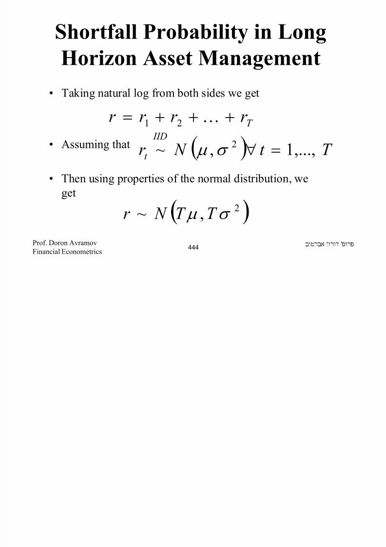
8/22/2019 Avramov Doron Financial Econometrics
http://slidepdf.com/reader/full/avramov-doron-financial-econometrics 444/553
Shortfall Probability and Long Horizon
• The normality assumption for log return implies the log
normal distribution for the cumulative return – more later.
• Let us understand the concept of shortfall probability.
• We ask: what is the probability that the investment yields a
return smaller than a threshold level (e.g., the riskfree rate)?
• To answer this question we need to compute the value of ariskfree investment over the T year period.
'Prof. Doron AvramovFinancial Econometrics
445
Shortfall Probability and Long Horizon

8/22/2019 Avramov Doron Financial Econometrics
http://slidepdf.com/reader/full/avramov-doron-financial-econometrics 445/553
Shortfall Probability and Long Horizon
• The value of such a riskfree investment is
where is the continuously compounded risk free rate.
( )T
f r RV V f
+= 10
f Tr V exp0=
f r
'Prof. Doron AvramovFinancial Econometrics
446
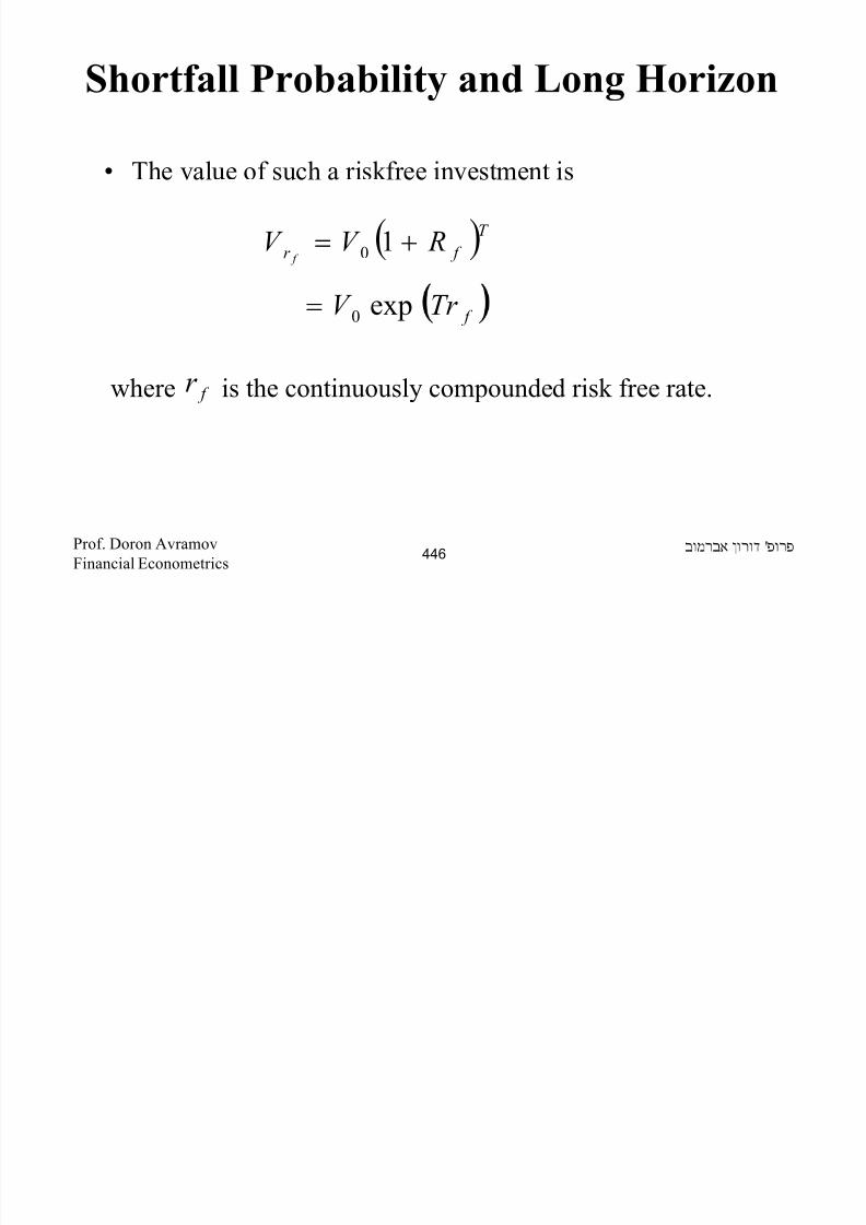
8/22/2019 Avramov Doron Financial Econometrics
http://slidepdf.com/reader/full/avramov-doron-financial-econometrics 446/553
Shortfall Probability and Long Horizon
• Essentially we ask: what is the probability that
• This is equivalent to asking what is the probability
that
• This, in turn, is equivalent to asking what is the
probability that
rf T
V V <
00 V
V
V V rf T <
<
00
lnlnV
V
V
V rf T
'Prof. Doron AvramovFinancial Econometrics
447
Shortfall Probability and Long Horizon
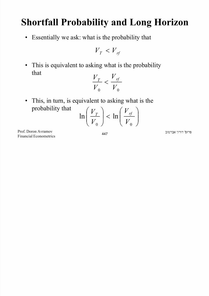
8/22/2019 Avramov Doron Financial Econometrics
http://slidepdf.com/reader/full/avramov-doron-financial-econometrics 447/553
Shortfall Probability and Long Horizon
• So we need to work out
• Subtracting and dividing by both sides of
the inequality we get
• We can denote this probability by
f Tr r p <
µ T σ T
−< σ
µ f
r T z P
−Φ=
σ
µ f r T Shortfall probabilit y
'Prof. Doron AvramovFinancial Econometrics
448
Shortfall Probability and long horizon

8/22/2019 Avramov Doron Financial Econometrics
http://slidepdf.com/reader/full/avramov-doron-financial-econometrics 448/553
Shortfall Probability and long horizon
• Typically which means the probability
diminishes the larger T .
• Notice that the shortfall probability can be written as a
function of the Sharpe ratio of log returns:
µ < f r
SRT SP −Φ=
'Prof. Doron AvramovFinancial Econometrics
449
Example

8/22/2019 Avramov Doron Financial Econometrics
http://slidepdf.com/reader/full/avramov-doron-financial-econometrics 449/553
Example
• Take r=0.04, µ=0.08, and σ=0.2 per year. What is the
Shortfall Probability for investment horizons of 1, 2, 5, 10,
and 20 years?
• Use the excel normdist function.
• If T=1 SP=0.42• If T=2 SP=0.39
• If T=5 SP=0.33
• If T=10 SP=0.26 • If T=20 SP=0.19
'Prof. Doron AvramovFinancial Econometrics
450
Cost of Insuring against Shortfall

8/22/2019 Avramov Doron Financial Econometrics
http://slidepdf.com/reader/full/avramov-doron-financial-econometrics 450/553
Cost of Insuring against Shortfall
• Let us now understand the mathematics of insuring against
shortfall.
• Without loss of generality let us assume that
• The investment value at time T is a given by the random
variable
10 =V
T V
'Prof. Doron AvramovFinancial Econometrics
451
Cost of Insuring against Shortfall

8/22/2019 Avramov Doron Financial Econometrics
http://slidepdf.com/reader/full/avramov-doron-financial-econometrics 451/553
Cost of Insuring against Shortfall
• Once we insure against shortfall the investment value
after T years becomes
– If you get
– If you get
T V f T Tr V exp>
f T Tr V exp< f Tr exp
'Prof. Doron AvramovFinancial Econometrics
452
Cost of Insuring against Shortfall

8/22/2019 Avramov Doron Financial Econometrics
http://slidepdf.com/reader/full/avramov-doron-financial-econometrics 452/553
Cost of Insuring against Shortfall
• So you essentially buy an insurance policy that pays 0
if
Pays if
• You ultimately need to price a contract with terminal
payoff given by
f T Tr V exp>
f T Tr V exp<T f V Tr −exp
T f V Tr −exp,0max
'Prof. Doron AvramovFinancial Econometrics
453
Cost of Insuring against Shortfall

8/22/2019 Avramov Doron Financial Econometrics
http://slidepdf.com/reader/full/avramov-doron-financial-econometrics 453/553
Cos o su g g s S o
• This is a European put option expiring in T years with
a. S=1
b. .
c. Riskfree rate given by
d. Volatility given by
e. Dividend yield given by
f Tr K exp=
f r
σ
0=δ
'Prof. Doron AvramovFinancial Econometrics
454
Cost of Insuring against Shortfall

8/22/2019 Avramov Doron Financial Econometrics
http://slidepdf.com/reader/full/avramov-doron-financial-econometrics 454/553
Cost of Insuring against Shortfall
• The B&S formula indicates that
• Which, given the parameter outlined above, becomes
( ) ( ) ( )12 expexp d N T S d N Tr K Put f −−−−−= δ
−−
= T N T N Put σ σ
2
1
2
1
'Prof. Doron AvramovFinancial Econometrics
455
Cost of Insuring against Shortfall
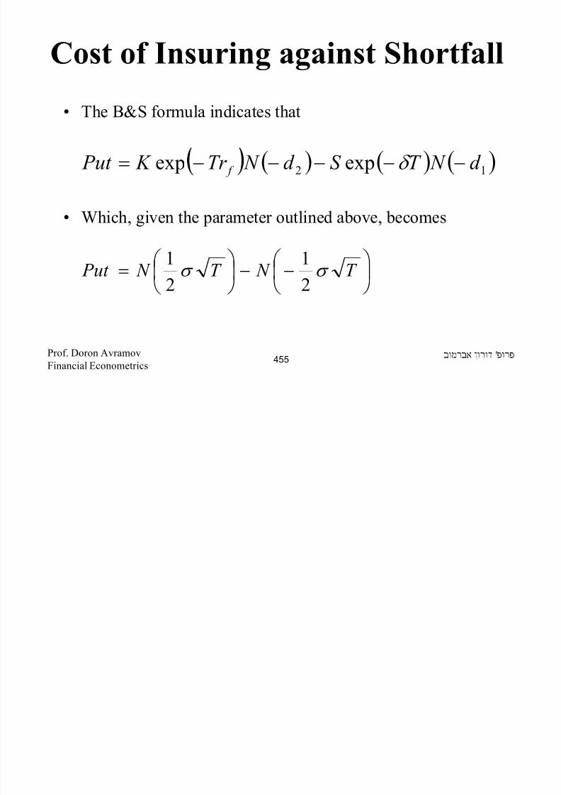
8/22/2019 Avramov Doron Financial Econometrics
http://slidepdf.com/reader/full/avramov-doron-financial-econometrics 455/553
Cost of Insuring against Shortfall
To show the pricing formula of the put use the following:
and
while
'Prof. Doron AvramovFinancial Econometrics
456
d ln S / K r T
T 1
21
2=+ − +( ) ( )δ σ
σd d T 2 1= − σ
( ) ( )
( ) ( )22
11
1
1
d N d N
d N d N
−=−
−=−
Cost of Insuring against Shortfall

8/22/2019 Avramov Doron Financial Econometrics
http://slidepdf.com/reader/full/avramov-doron-financial-econometrics 456/553
g g
• The B&S option-pricing model gives the current put
price P as
where
and is
( ) ( )21 d N d N Put −=
12
12
d d
T d
−=
= σ
( )d N d z prob <
'Prof. Doron AvramovFinancial Econometrics
457
Cost of Insuring against Shortfall
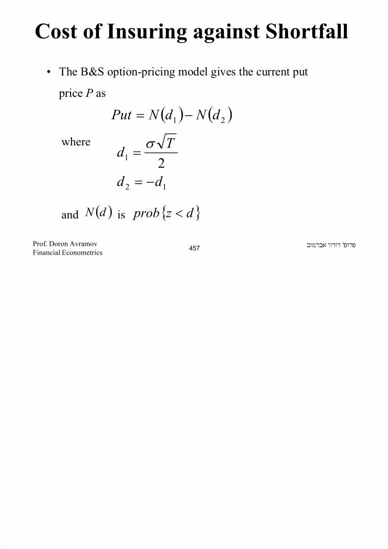
8/22/2019 Avramov Doron Financial Econometrics
http://slidepdf.com/reader/full/avramov-doron-financial-econometrics 457/553
Cos o su g g s S o
• For (per year)2.0=σ PT (years)
0.081
0.185
0.2510
0.35200.4230
0.5250
'Prof. Doron AvramovFinancial Econometrics458
Cost of Insuring against Shortfall

8/22/2019 Avramov Doron Financial Econometrics
http://slidepdf.com/reader/full/avramov-doron-financial-econometrics 458/553
g g
• We have found out that the cost of the insurance increases
in T , even when the probability of shortfall decreases in T
(as long as the Sharpe ratio is positive).
• To get some idea about this apparently surprising outcome
it would be essential to discuss the expected value of the
investment payoff given the shortfall event.
• It is a great opportunity to understand down side risk when
the underlying distribution is log normal rather than
normal.
'Prof. Doron AvramovFinancial Econometrics459
The Expected Value of

8/22/2019 Avramov Doron Financial Econometrics
http://slidepdf.com/reader/full/avramov-doron-financial-econometrics 459/553
p
Cumulative Return• Two proper questions emerge at this stage:
1. What is the expected value of cumulative return during
the investment horizon ?
2. What is the conditional expectation – conditional on
shortfall ?
• We assume, without loss of generality, that the initial
invested wealth is one.
)( T V E
)exp(| f T T Tr V V E <
'Prof. Doron AvramovFinancial Econometrics460
The Expected Value of

8/22/2019 Avramov Doron Financial Econometrics
http://slidepdf.com/reader/full/avramov-doron-financial-econometrics 460/553
p
Cumulative Return• Notice that, given the tools we have acquired thus far,
finding the conditional expectation is a nontrivial task
since is not normally distributed – rather it is log-
normally distributed since.
• Thus, let us first display some properties of the log normal
distribution.
),(~)ln( 2σ µ T T N V T
T V
'Prof. Doron AvramovFinancial Econometrics 461
The Log Normal Distribution

8/22/2019 Avramov Doron Financial Econometrics
http://slidepdf.com/reader/full/avramov-doron-financial-econometrics 461/553
g
• Suppose that x has the log normal distribution. Then the
parameters µ and σ are, respectively, the mean and the
standard deviation of the variable’s natural logarithm,
which means
where z is a standard normal variable.
• The probability density function of a log-normal
distribution is
z
e xσ µ +
=
'Prof. Doron AvramovFinancial Econometrics 462
The Log Normal Distribution

8/22/2019 Avramov Doron Financial Econometrics
http://slidepdf.com/reader/full/avramov-doron-financial-econometrics 462/553
g
• If x is a log-normally distributed variable, its expected
value and variance are given by
( )( )
0,2
1,,
2
2
2
ln
>Π
=−
− xe
x x f
x
xσ
µ
σ σ µ
[ ]
[ ] ( ) ( ) [ ]( )22
2
1
11222
2
x E eee xVar
e x E
−=−=
=+
+
σ σ µ σ
σ µ
'Prof. Doron AvramovFinancial Econometrics 463
The Mean and Variance of T V

8/22/2019 Avramov Doron Financial Econometrics
http://slidepdf.com/reader/full/avramov-doron-financial-econometrics 463/553
• Using moments of the log normal distribution, the mean
and variance of are
• Next, we aim to find the conditional mean.
( )1)exp()2exp()(
)2
1exp()(
22
2
−+=
+=
σ σ µ
σ µ
T T T V Var
T T V E
T
T
T V
'Prof. Doron AvramovFinancial Econometrics 464
The Mean of a Variable that has the
Truncated Log Normal Distribution

8/22/2019 Avramov Doron Financial Econometrics
http://slidepdf.com/reader/full/avramov-doron-financial-econometrics 464/553
Truncated Log Normal Distribution
where is a normalizing constant.
• Let us make change of variables:
( )( )
∫
∞
−
−
=c
ln
2
12
2x
1xc)>x|E(xcF dxe
x
σ
µ
π σ
( )cF1/
dte=dxand e=xt-ln(x) tt µ σ µ σ σ
σ
µ ++⇒=
'Prof. Doron AvramovFinancial Econometrics 465
The Mean of a Variable that has the
Truncated Log Normal Distribution

8/22/2019 Avramov Doron Financial Econometrics
http://slidepdf.com/reader/full/avramov-doron-financial-econometrics 465/553
Truncated Log Normal Distribution
then: ( ) ( )
( )
( ) ( )( )
( )( )
( )∫
∫
∫
∫
∞
−
−−
+
∞−
++−−
∞
−
++−
∞
−+−
Π=
Π=
Π=
=Π
=
σ
µ
σ
σ µ
σ
µ
σ µ σ
σ
µ
µ σ
σ
µ µ σ σ
σ
cln 2
1
5.0
cln
5.021
cln2
1
cln2
1
22
22
2
2
21
2
1
2
1
2x
1c)>x|E(xcF
dt ee
dt e
dt e
dt ee
t
t
t t
t t
'Prof. Doron AvramovFinancial Econometrics 466
The Mean of a Variable that has the
Truncated Log Normal Distribution

8/22/2019 Avramov Doron Financial Econometrics
http://slidepdf.com/reader/full/avramov-doron-financial-econometrics 466/553
Truncated Log Normal Distribution
• Let us make another change of variables:
• The integral is the complement CDF of the standard normal
random variable.
( )( )
( )
∫
∞
−−
−+
Π= σ σ
µ
σ µ
cln
2
1
5.02
2
2
1
c)>x|E(xcF dvee
v
dt=dv-t=v ⇒σ
'Prof. Doron Avramov
Financial Econometrics 467
The Mean of a Variable that has the
Truncated Log Normal Distribution

8/22/2019 Avramov Doron Financial Econometrics
http://slidepdf.com/reader/full/avramov-doron-financial-econometrics 467/553
Truncated Log Normal Distribution
• Thus, the formula is reduced to:
( ) ( ) ( )
( ) ( )
++−
Φ=
−−Φ−=
+
+
σ
σ µ
σ σ µ
σ µ
σ µ
25.0
2
5.0LN
ln
ln1c)>x|(xEcF
2
2
c
e
ce
'Prof. Doron Avramov
Financial Econometrics 468
The Mean of a Variable that has the
Truncated Log Normal Distribution

8/22/2019 Avramov Doron Financial Econometrics
http://slidepdf.com/reader/full/avramov-doron-financial-econometrics 468/553
Truncated Log Normal Distribution
• In the same way we can show that:
( )( ) ( )
( ) ( )( )
( )( )
( ) ( )
−−Φ⋅=
Π=Π=
=Π⋅
=≤⋅
+
−−
∞−
−+−
∞−
−−+
−
∞−
++−
−−
∫∫
∫∫
σ
σ µ
σ
σ µ
σ σ
µ
σ µ σ
µ σ
σ µ
σ
µ µ σ
σ µ
25.0
ln
2
1
5.0
ln
2
1
5.0
ln
2
1ln21
0LN
ln
2
1
2
1
2
1c)x|(xEcF
2
22
22
2
2
ce
dveedt ee
dt edxe x
x
cv
ct
ct t
xc
'Prof. Doron Avramov
Financial Econometrics 469
Punch Lines

8/22/2019 Avramov Doron Financial Econometrics
http://slidepdf.com/reader/full/avramov-doron-financial-econometrics 469/553
( )
( )
+−Φ
++−Φ
⋅=>σ
µ
σ
σ µ
c
c
ln
ln
(x)Ec)x|(xE
2
LNLN
( )
( )
−Φ
−−Φ
⋅=≤
σ
µ
σ σ µ
c
c
ln
ln
(x)Ec)x|(xE
2
LNLN
'Prof. Doron Avramov
Financial Econometrics 470
The Expected Value given Shortfall

8/22/2019 Avramov Doron Financial Econometrics
http://slidepdf.com/reader/full/avramov-doron-financial-econometrics 470/553
• The expected value given shortfall is
or
• Notice that the denominator is the shortfall probability.
[ ]
−Φ
−−Φ
⋅=
+
σ
µ σ
σ µ
σ µ
T
T Tr T
T T Tr
e shortfall V E f
f
T T
T
2
2
12
|
[ ]( )( )
( )SRT
SRT e shortfall V E
T T
T ⋅−Φ
+−Φ⋅=
+ σ σ µ 2
2
1
|
'Prof. Doron Avramov
Financial Econometrics 471
The Expected Value given Shortfall

8/22/2019 Avramov Doron Financial Econometrics
http://slidepdf.com/reader/full/avramov-doron-financial-econometrics 471/553
• Thus,
• Which means that the shortfall probability times the expected
value given shortfall is equal to the unconditional expected
value times a factor smaller than one.
• That factor diminishes with higher Sharpe ratio and/or with
higher volatility.
[ ] ( )σ +−Φ=× SRT V E shortfall V E shortfall ob t T ][|)(Pr
'Prof. Doron Avramov
Financial Econometrics 472
The Horizon Effect

8/22/2019 Avramov Doron Financial Econometrics
http://slidepdf.com/reader/full/avramov-doron-financial-econometrics 472/553
Numerical example
• Let’s take . For different values of the conditional expectation over horizon T looks like:
%10%,5 == σ f r f r >µ
'Prof. Doron Avramov
Financial Econometrics 473
The Horizon Effect

8/22/2019 Avramov Doron Financial Econometrics
http://slidepdf.com/reader/full/avramov-doron-financial-econometrics 473/553
• Previously we have shown that even when the shortfall
probability diminishes with the investment horizon, the costof insuring against shortfall rises.
• Notice that the insured amount is
• The expected value of that insured amount given shortfall
sharply rises with the investment horizon, which explains the
increasing value of the put option.
T f V Tr −exp
'Prof. Doron Avramov
Financial Econometrics 474
Value at Risk with Log Normal

8/22/2019 Avramov Doron Financial Econometrics
http://slidepdf.com/reader/full/avramov-doron-financial-econometrics 474/553
Distribution
• We have analyzed VaR when quantities of interest arenormally distributed.
• It is challenging to extend the analysis to the case wherein the
log normal distribution is considered.
• Analytics follow.
'Prof. Doron Avramov
Financial Econometrics 475
VaR with Log Normal Distribution

8/22/2019 Avramov Doron Financial Econometrics
http://slidepdf.com/reader/full/avramov-doron-financial-econometrics 475/553
• We are looking for threshold, VaR, such that
• Then in order to find the threshold we need to calculate
quantile of lognormal distribution:
where is as defined earlier.
( ) ( )000Pr V VaRCDF V Var V V T =<=α
( )21
0 ,; σ µ α T T CDF V VaR −⋅=
( )α σ µ 1
0
−Φ⋅+
⋅=
T T
eV ( )α 1−Φ
'Prof. Doron Avramov
Financial Econometrics 476
VaR with Log Normal Distribution

8/22/2019 Avramov Doron Financial Econometrics
http://slidepdf.com/reader/full/avramov-doron-financial-econometrics 476/553
• Specifically,
( ) ( ) ( )( )0000 lnlnPr Pr V VaRV V V Var V V T T <=<=α
( ) ( )
−<
−=
σ
µ
σ
µ
T
T V VaR
T
T V V T 00 lnlnPr
( )
−Φ=
σ
µ
T
T V VaR 0ln
'Prof. Doron Avramov
Financial Econometrics 477
VaR with Log Normal Distribution

8/22/2019 Avramov Doron Financial Econometrics
http://slidepdf.com/reader/full/avramov-doron-financial-econometrics 477/553
and then
That is to say that there is a α% probability that the investment
value at time T will be below that VaR.
( )( )
( )α σ µ
α σ
µ
1
0
10ln
−Φ⋅+
−
=
Φ=
−
T T eV VaR
T
T V VaR
'Prof. Doron Avramov
Financial Econometrics 478
VaR with t Distribution

8/22/2019 Avramov Doron Financial Econometrics
http://slidepdf.com/reader/full/avramov-doron-financial-econometrics 478/553
• Suppose now that stock returns have a t
distribution with ν degrees of freedom and
expected return and volatility given by and σ
• The pdf of stock return is formulated as
'Prof. Doron Avramov
Financial Econometrics 479
( ) ( )
2
12)(
121,2
1,,|
+−
−+⋅⋅=
v
v
x
v Bvv x f
µ
σ σ µ
Partial Expectation

8/22/2019 Avramov Doron Financial Econometrics
http://slidepdf.com/reader/full/avramov-doron-financial-econometrics 479/553
• Let -standardized r.v distribution with .
Than,
'Prof. Doron Avramov
Financial Econometrics 480
( ) ( )( )
=
+⋅
⋅=⋅=≤
+−
∞−∞− ∫∫ dxv
x
v Bvdxv x f x z X X PE
v
z z 2
1
2
121,2
1,|
( )
( )( )
1,1
121,2
1
|1121,2
1
212
1
2
2
1
2
−+⋅−=
+
−−⋅
⋅
=
+
−−⋅
⋅=
+
+
−
∞−
−−
v
z vv z f
v
z
v
v
v Bv
v x
vv
v Bv
v
z
v
σ
µ −= xY ( )v x F ,1,0|
Partial Expectation

8/22/2019 Avramov Doron Financial Econometrics
http://slidepdf.com/reader/full/avramov-doron-financial-econometrics 480/553
And thus
Where is x quantile of
'Prof. Doron Avramov
Financial Econometrics 481
( ) ( )1
, 21
1
1
−+⋅−= −
−
−
v
qv
q
vq f ES T α
α
α σ µ α
( ) xVaRq x −= 1 nt T ~
Long Run Return when Periodic

8/22/2019 Avramov Doron Financial Econometrics
http://slidepdf.com/reader/full/avramov-doron-financial-econometrics 481/553
The sum of independent t-distributed random variables is not t-
distributed. So we have no nice formula for expected shortfall
in the long run. However, it can be approximated by normal
with zero mean variance:
Return has the t- Distribution
'Prof. Doron Avramov
Financial Econometrics 482
−σ µ
2,~
. v
v N r
approx for 2≥v
Long Run Return when Periodic
R h h Di ib i

8/22/2019 Avramov Doron Financial Econometrics
http://slidepdf.com/reader/full/avramov-doron-financial-econometrics 482/553
• Approximation makes sense for large v’s when t coincides
with normal distribution.
• However, simulation studies show that for sufficient
number of periods this approximation works well enough.
Return has the t- Distribution
'Prof. Doron Avramov
Financial Econometrics 483
Long Run Return when Periodic
R h h Di ib i

8/22/2019 Avramov Doron Financial Econometrics
http://slidepdf.com/reader/full/avramov-doron-financial-econometrics 483/553
• However simulations shows that for sufficient number of
periods this approximation works well enough.
• Let . The next graphs show normal
curve fit to the sum of t r.v.s (over T periods); sampleestimates vs. predicted parameters are includes
Return has the t- Distribution
'Prof. Doron Avramov
Financial Econometrics 484
05.0;01.0 == t t σ µ
Long Run Return when Periodic
R t h th t Di t ib ti

8/22/2019 Avramov Doron Financial Econometrics
http://slidepdf.com/reader/full/avramov-doron-financial-econometrics 484/553
Return has the t- Distribution
'Prof. Doron Avramov
Financial Econometrics 485
-3 -2 -1 0 1 2 30
100
200
300
400
500
600
700
800
900
10=T
274.01.0
==
N
N
σ µ
273.0ˆ
102.0ˆ
==
σ
µ
3=v
Long Run Return when Periodic
R t h th t Di t ib ti

8/22/2019 Avramov Doron Financial Econometrics
http://slidepdf.com/reader/full/avramov-doron-financial-econometrics 485/553
-4 -3 -2 -1 0 1 2 3 4 50
50
100
150
200
250
300
350
400
Return has the t- Distribution
'Prof. Doron Avramov
Financial Econometrics 486
100=T
866.0
1
=
=
N
N
σ
µ
856.0ˆ011.1ˆ
==
σ µ
3=v
Long Run Return when Periodic
R t h th t Di t ib ti

8/22/2019 Avramov Doron Financial Econometrics
http://slidepdf.com/reader/full/avramov-doron-financial-econometrics 486/553
-0.6 -0.4 -0.2 0 0.2 0.4 0.6 0.80
50
100
150
200
250
300
350
Return has the t- Distribution
'Prof. Doron Avramov
Financial Econometrics 487
10=T
177.01.0
==
N
N
σ µ
174.0ˆ
099.0ˆ
==
σ
µ
10=v
Long Run Return when Periodic
R t h th t Di t ib ti

8/22/2019 Avramov Doron Financial Econometrics
http://slidepdf.com/reader/full/avramov-doron-financial-econometrics 487/553
-1 -0.5 0 0.5 1 1.5 2 2.5 3 3.50
50
100
150
200
250
300
350
Return has the t- Distribution
'Prof. Doron Avramov
Financial Econometrics 488
100=T
559.01
== N
N
σ µ
566.0ˆ994.0ˆ
==σ µ
10=v
VaR Expected Shortfall using Extreme
Val e Theorem (EVT) Witho t

8/22/2019 Avramov Doron Financial Econometrics
http://slidepdf.com/reader/full/avramov-doron-financial-econometrics 488/553
• Estimating VaR and ES using EVT can be done in two
ways:
• The idea of sub-periods;
• The idea based on exceedances over a threshold.
• Both ideas are based on assumption that extreme events of
many distributions (normal, student-t etc.) are distributed
with one of the extreme value distributions family. There isa lot of material on an issue and jut summarized the most
important points.
Value Theorem (EVT) - WithoutDistribution Assumption
'Prof. Doron Avramov
Financial Econometrics 489
• Divide the sample into m non overlapping subsamples (to
Sub-Periods

8/22/2019 Avramov Doron Financial Econometrics
http://slidepdf.com/reader/full/avramov-doron-financial-econometrics 489/553
• Divide the sample into m non-overlapping subsamples (to preserve iid assumption) of length n:
• Then using minimum of each sub-period estimate GEV
density of the following form
'Prof. Doron Avramov
Financial Econometrics 490
mnmnnnn r r r r r r KKKK 1211 ||| ++
( )
( )
wher e
e
z GEV z
z
e
z
,
0,1
1
≠
= −
+− −
ξ ξ
0, ≠ξ σ
µ −=
x z
• Using estimations of and we can compute VaR
Sub-Periods
nn µξ nσ

8/22/2019 Avramov Doron Financial Econometrics
http://slidepdf.com/reader/full/avramov-doron-financial-econometrics 490/553
• Using estimations of and we can compute VaR
• Here we used the assumption that returns are iid and thensingle period return is related to return over sub-period n as
follows
'Prof. Doron Avramov
Financial Econometrics 491
( )
( )[ ]
( )[ ]
−⋅−+
≠−−⋅−+
=
−
α σ µ
ξ α
ξ
σ µ
α
ξ
1lnln
0,11ln
n
n
VaR
nn
n
n
nn
n
0, ≠nξ
( ) ( ) ( )[ ]nn
t
nnn cr P cr P cr P ∏=
<=<=<1
nn µ ξ , nσ
• The result of the EVT are also relevant for the task of
Long Term VaR
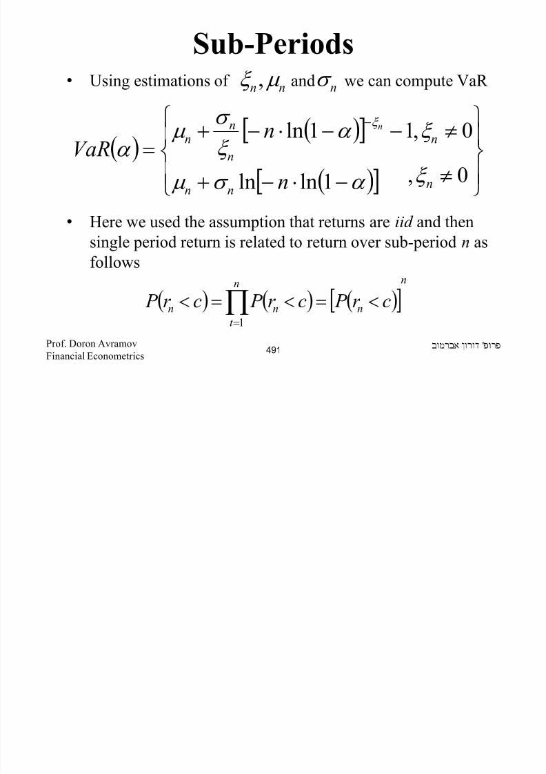
8/22/2019 Avramov Doron Financial Econometrics
http://slidepdf.com/reader/full/avramov-doron-financial-econometrics 491/553
• The result of the EVT are also relevant for the task of converting short-term VaR into long-term VaR. Assume
applies to a single-period return for large R.
Then we have for a T-period return
• It follows that a multi-period VaR forecast of a fat tailed
return distribution under the iid assumption is given by
'Prof. Doron Avramov
Financial Econometrics 492
ξ 1
1
~ −
≤≤
⋅
≤∑ RT Rr P
T t
t
( ) ( )α α ξ 11 VaRT VaR T ⋅= −
( ) ξ 1~ −≤ R Rr P
Exceedances over a Threshold
F i h h ld h di i l di ib i

8/22/2019 Avramov Doron Financial Econometrics
http://slidepdf.com/reader/full/avramov-doron-financial-econometrics 492/553
'Prof. Doron Avramov
Financial Econometrics 493
( ( hl yhl P y F h >≤−= | for hl y F −≤≤0
( )( (
( ) y F
y F yh F y F h
−
−+=
1
)1(
• For a given threshold h conditional excess distribution
function on losses is defined as
• In terms of F this can be written as
• For a large class of underlying distribution functions F the
Exceedances over a Threshold

8/22/2019 Avramov Doron Financial Econometrics
http://slidepdf.com/reader/full/avramov-doron-financial-econometrics 493/553
For a large class of underlying distribution functions F theconditional excess distribution function , for h large,
is well approximated by generalized Pareto distribution:
• For
( ) y F h
'Prof. Doron Avramov
Financial Econometrics 494
( )
−
≠
+−
=
−
−
σ
ξ
ξ σ
ξ
ye
y
yGP
1
0,111
0, ≠ξ
0≥ξ [ ]hl z F −∈ ,0 if and [ ]ξ σ −,0 if 0<ξ
• Using this model VaR and ES can be expressedl ti ll
Long Horizon VaR

8/22/2019 Avramov Doron Financial Econometrics
http://slidepdf.com/reader/full/avramov-doron-financial-econometrics 494/553
Using this model VaR and ES can be expressedanalytically:
First, using (1) we can isolate
• Then is replaced by GP CDF and F(h) by the sample
estimate , where n is the total number of
observations and is the number of exceedances above
the threshold h:
( ) y F h
( )n N n h−
h N
( )l F
'Prof. Doron Avramov
Financial Econometrics 495
( ([ ] ( (h F y F h F l F h +−= 1
( ) ( )( ) ξ ξ
111
−−+−= hl n
N l F h
• Next
Long Horizon VaR
ξ

8/22/2019 Avramov Doron Financial Econometrics
http://slidepdf.com/reader/full/avramov-doron-financial-econometrics 495/553
Next
And
is mean excess function for GP distribution which
equals to
'Prof. Doron Avramov
Financial Econometrics 496
( ) ( )
−
+==
−
− 11
ξ
ξ
σ α α
h N
nh F VaR
( ( ( (( α α α α VaRl VaRl E VaR ES >−+= |
Long Horizon VaR

8/22/2019 Avramov Doron Financial Econometrics
http://slidepdf.com/reader/full/avramov-doron-financial-econometrics 496/553
'Prof. Doron Avramov
Financial Econometrics 497
( )( )
ξ
ξ σ
ξ
α α
+
−+
+
=
11
hVaR ES
• Given a s sample and some threshold h, parameters , andcan be estimated using MLE. σ ξ
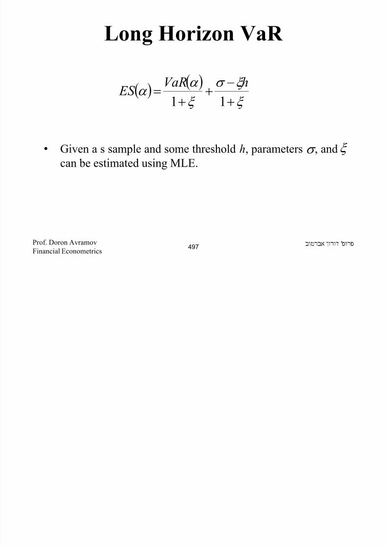
8/22/2019 Avramov Doron Financial Econometrics
http://slidepdf.com/reader/full/avramov-doron-financial-econometrics 497/553
Class Notes in
Financial Econometrics
Testing the Black&ScholesFormula
'Prof. Doron Avramov
Financial Econometrics 498
Option Pricing

8/22/2019 Avramov Doron Financial Econometrics
http://slidepdf.com/reader/full/avramov-doron-financial-econometrics 498/553
d ln S / K r T
T
1
21
2=+ − +( ) ( )δ σ
σ
d d T 2 1= − σ
C S,K, ,r,T, Se N d Ke N d - T -rT ( ) = ( ) ( )σ δ δ1 2−
P S,K, ,r,T, Ke N d Se N d -rT - T ( ) = ( ) ( )σ δ δ− − −2 1
• The B&S call Option price is given by
• The put Option price is
Where and
'Prof. Doron Avramov
Financial Econometrics 499
Option Pricing

8/22/2019 Avramov Doron Financial Econometrics
http://slidepdf.com/reader/full/avramov-doron-financial-econometrics 499/553
• There are six inputs required:
S- Current price of the underlying asset.K- Exercise/Strike price.
r- Continuously compounded riskfree rate.
T- Time to expiration.
- Volatility.
- Continuously compounded dividend yield.
σ
δ
'Prof. Doron Avramov
Financial Econometrics 500
The B&S Economy

8/22/2019 Avramov Doron Financial Econometrics
http://slidepdf.com/reader/full/avramov-doron-financial-econometrics 500/553
• The B&S formula is derived under several assumptions:
• The stock price follows a geometric Brownian motion(continuous path and continuous time).
• The dividend is paid continuously and uniformly over
time.
• The interest rate is constant over time.
'Prof. Doron Avramov
Financial Econometrics 501
The B&S Economy

8/22/2019 Avramov Doron Financial Econometrics
http://slidepdf.com/reader/full/avramov-doron-financial-econometrics 501/553
• The underlying asset volatility is constant over time
and it does not change with the option maturity or with
the strike price.
• You can short sell or long any amount of the stock.
• You can borrow and lend in the riskfree rate.
• There are no transactions costs.
'Prof. Doron Avramov
Financial Econometrics502
Testing the B&S Formula
M k R bi t i l ll ti th t d t f

8/22/2019 Avramov Doron Financial Econometrics
http://slidepdf.com/reader/full/avramov-doron-financial-econometrics 502/553
• Mark Rubinstein analyzes call options that are deep out of
the money.
• He considers matched pairs: options with the same striking
price, on the same underlying asset (stock), but with
different time to maturity (expiration date).
• He examines overall 373 pairs.
• If B&S is correct then the implied volatility (IV) of thematched pair is equal. Time to maturity plays no role.
'Prof. Doron Avramov
Financial Econometrics503
Testing the B&S Formula
H R bi t i fi d th t f th 373 i d

8/22/2019 Avramov Doron Financial Econometrics
http://slidepdf.com/reader/full/avramov-doron-financial-econometrics 503/553
• However, Rubinstein finds that our of the 373 examined
matched pairs – shorter maturity options had higher IV.
• Under the null – the expected value of such an outcome is
373/2=186.5.
• Is the difference statistically significant?
'Prof. Doron Avramov
Financial Econometrics504
The Failure Rate based Test
Statistic

8/22/2019 Avramov Doron Financial Econometrics
http://slidepdf.com/reader/full/avramov-doron-financial-econometrics 504/553
•Use the failure rate test developed earlier to show that time to
expiration does play a major role.
•That is to say that the constant volatility assumption is
strongly violated in the data.
'Prof. Doron Avramov
Financial Econometrics505
The Volatility Smile for Foreign
Currency Options

8/22/2019 Avramov Doron Financial Econometrics
http://slidepdf.com/reader/full/avramov-doron-financial-econometrics 505/553
Currency Options
'Prof. Doron Avramov
Financial Econometrics506
Implied
Volatility
Strike
Price
Implied Distribution for
Foreign Currency Options

8/22/2019 Avramov Doron Financial Econometrics
http://slidepdf.com/reader/full/avramov-doron-financial-econometrics 506/553
g y p
•Both tails are heavier than the lognormal distribution.
•It is also “more peaked” than the lognormal distribution.
'Prof. Doron Avramov
Financial Econometrics507
The Volatility Smile for Equity
Options
8/22/2019 Avramov Doron Financial Econometrics
http://slidepdf.com/reader/full/avramov-doron-financial-econometrics 507/553
p
'Prof. Doron Avramov
Financial Econometrics508
Implied
Volatility
Strike
Price
Implied Distribution for Equity
Options

8/22/2019 Avramov Doron Financial Econometrics
http://slidepdf.com/reader/full/avramov-doron-financial-econometrics 508/553
p
•The left tail is heavier and the right tail is less heavy than thelognormal distribution.
'Prof. Doron Avramov
Financial Econometrics509
Ways of Characterizing the
Volatility Smiles

8/22/2019 Avramov Doron Financial Econometrics
http://slidepdf.com/reader/full/avramov-doron-financial-econometrics 509/553
y•Plot implied volatility against K/S0 (The volatility smile is
then more stable).•Plot implied volatility against K/F0 (Traders usually define an
option as at-the-money when K equals the forward price, F0,
not when it equals the spot price S0).
•Plot implied volatility against delta of the option (This
approach allows the volatility smile to be applied to some non-
standard options. At-the money is defined as a call with a delta
of 0.5 or a put with a delta of −0.5. These are referred to as 50-delta options).
'Prof. Doron Avramov
Financial Econometrics510
Possible Causes of Volatility
Smile

8/22/2019 Avramov Doron Financial Econometrics
http://slidepdf.com/reader/full/avramov-doron-financial-econometrics 510/553
• Asset price exhibits jumps rather than continuous changes.
• Volatility for asset price is stochastic:
- In the case of an exchange rate volatility is not heavily
correlated with the exchange rate. The effect of a
stochastic volatility is to create a symmetrical smile.
- In the case of equities volatility is negatively related to s
stock prices because of the impact of leverage. This isconsistent with the skew that is observed in practice.
'Prof. Doron Avramov
Financial Econometrics511
Volatility Term Structure

8/22/2019 Avramov Doron Financial Econometrics
http://slidepdf.com/reader/full/avramov-doron-financial-econometrics 511/553
•In addition to calculating a volatility smile, traders also
calculate a volatility term structure.
•This shows the variation of implied volatility with the time to
maturity of the option.
•The volatility term structure tends to be downward sloping
when volatility is high and upward sloping when it is low
'Prof. Doron Avramov
Financial Econometrics512
Example of a Volatility Surface
K /S 0
0 90 0 95 1 00 1 05 1 10

8/22/2019 Avramov Doron Financial Econometrics
http://slidepdf.com/reader/full/avramov-doron-financial-econometrics 512/553
'Prof. Doron Avramov
Financial Econometrics513
0.90 0.95 1.00 1.05 1.10
1 mnth 14.2 13.0 12.0 13.1 14.5
3 mnth 14.0 13.0 12.0 13.1 14.2
6 mnth 14.1 13.3 12.5 13.4 14.3
1 year 14.7 14.0 13.5 14.0 14.8
2 year 15.0 14.4 14.0 14.5 15.1
5 year 14.8 14.6 14.4 14.7 15.0
Class Notes in

8/22/2019 Avramov Doron Financial Econometrics
http://slidepdf.com/reader/full/avramov-doron-financial-econometrics 513/553
Class Notes in
Financial Econometrics
Time Varying Volatility Models
'Prof. Doron Avramov
Financial Econometrics514
Volatility Models
• We describe several volatility models commonly applied in

8/22/2019 Avramov Doron Financial Econometrics
http://slidepdf.com/reader/full/avramov-doron-financial-econometrics 514/553
y y pp
analyzing quantities of interest in finance and economics:
• ARCH
• GARCH
• EGARCH
• Stochastic Volatility
• Realized and implied Volatility
'Prof. Doron Avramov
Financial Econometrics515
Volatility Models
• All such models attempt to capture the empirical evidence

8/22/2019 Avramov Doron Financial Econometrics
http://slidepdf.com/reader/full/avramov-doron-financial-econometrics 515/553
that volatility is time varying (rather than constant) as well
as persistent.
• The EGARCH captures the asymmetric response of
volatility to advancing versus diminishing markets.
• In particular, volatility tends to be higher (lower) during
down (up) markets.
'Prof. Doron Avramov
Financial Econometrics516
h
ARCH(1)
( )10N=+= t t
er
σεε µ

8/22/2019 Avramov Doron Financial Econometrics
http://slidepdf.com/reader/full/avramov-doron-financial-econometrics 516/553
where ( )1,0~ N et
2221
21 t t t t t t e E E σ σ ε == −−
2
1
2
−+=
=
t t
t t t
w
e
αε σ
σ ε
so
is the conditional variance.2t σ
'Prof. Doron Avramov
Financial Econometrics517
ARCH (1)22
1 σ ε =−t E is the unconditional variance.

8/22/2019 Avramov Doron Financial Econometrics
http://slidepdf.com/reader/full/avramov-doron-financial-econometrics 517/553
2
1
2
−+= t t w E E αε σ
2
1−+= t E w ε α
2
1
2
1 −−+= t t e E E w σ α
( )21−+= t E w σ α
2
2
2
1
22
−− ===⇒ t t t E E E σ σ σ σ
( )α
σ −
=1
2 w E t
'Prof. Doron Avramov
Financial Econometrics
518
ARCH (1)
( ) ( )[ ]• Fat tail?

8/22/2019 Avramov Doron Financial Econometrics
http://slidepdf.com/reader/full/avramov-doron-financial-econometrics 518/553
( )
( )
( )[ ]
( )[ ]2
221
4
1
22
4
4
t t t
t t
t
t
e E E
E E
E
E
σ
ε
ε
ε µ
+==
−
−
( )( )( )[ ]
( )( )( )
( )
( )( )33
3
3
22
4
22
4
222
1
44
1
≥=
=+= −
−
t
t
t
t
t t t
t t t
E
E
E
E
e E E
e E E
σ
σ
σ
σ
σ
σ
'Prof. Doron Avramov
Financial Econometrics
519
ARCH (1)
• The last step follows because:

8/22/2019 Avramov Doron Financial Econometrics
http://slidepdf.com/reader/full/avramov-doron-financial-econometrics 519/553
( ) ( ) ( ) 02242 ≥−= t t t E E Var ε ε ε
so
• Yes – fat tail!
(
( )
122
4
≥t
t
E
E
ε
ε
'Prof. Doron Avramov
Financial Econometrics
520
h
GARCH(1,1)
( )10~ Ne+= t t
e
r
σε
ε µ

8/22/2019 Avramov Doron Financial Econometrics
http://slidepdf.com/reader/full/avramov-doron-financial-econometrics 520/553
where ( )1,0~ N et
( ) ( ) ( )2
1
2
1
2
2
1
2
1
2
−−
−−
++=
++=
=
t t t
t t t
t t t
E E w E
w
e
σ β ε α σ
βσ αε σ
σ ε
'Prof. Doron Avramov
Financial Econometrics
521
GARCH(1,1)
222 ++= σ β σ α σ w

8/22/2019 Avramov Doron Financial Econometrics
http://slidepdf.com/reader/full/avramov-doron-financial-econometrics 521/553
( )( )3
321
113
1
1
224
2
>−−−
−−++=
−−=
β α αβ
β α β α µ
β α σ
'Prof. Doron Avramov
Financial Econometrics
522
where
EGARCH
( )1,0~ N et
=+= t t
e
r
σε
ε µ

8/22/2019 Avramov Doron Financial Econometrics
http://slidepdf.com/reader/full/avramov-doron-financial-econometrics 522/553
•The first component
is the absolute value of a normally distribution variable
minus its expectation.
( ) ( )2
1
1
1
1
12 ln2ln −−
−
−
− +−
−+=
=
t
t
t
t
t t
t t t
w
e
σ β σ ε γ
π σ ε α σ
σ ε
π π σ ε 22
1
1
1 −=
− −
−
−t
t
t e
1−t e
'Prof. Doron Avramov
Financial Econometrics
523
•The second component is
EGARCH
1
1
1−
−
− = t
t
t eγ σ ε γ
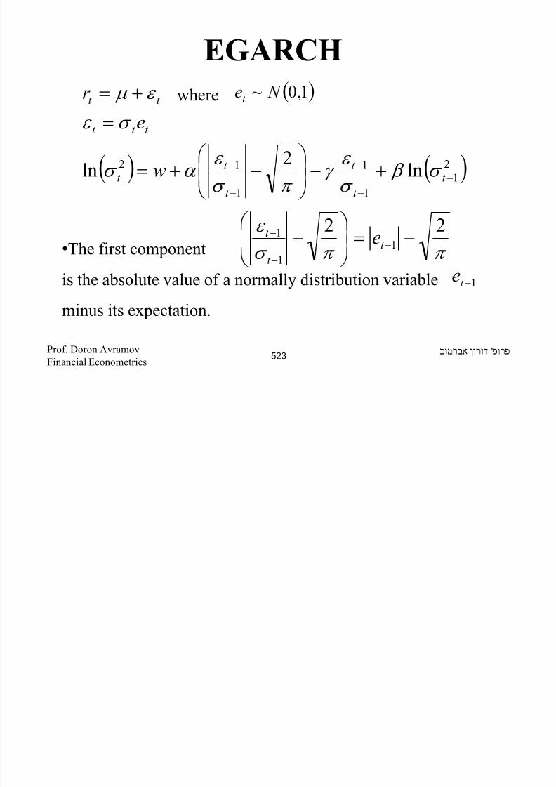
8/22/2019 Avramov Doron Financial Econometrics
http://slidepdf.com/reader/full/avramov-doron-financial-econometrics 523/553
• Notice that the two normal shocks behave differently.
•The first produces a symmetric rise in the log conditional
variance.
•The second creates an asymmetric effect, in that, the log
conditional variance rises following a negative shock.
1−t
'Prof. Doron Avramov
Financial Econometrics
524
•More formally if then the log conditional variance
EGARCH
01 <−t e

8/22/2019 Avramov Doron Financial Econometrics
http://slidepdf.com/reader/full/avramov-doron-financial-econometrics 524/553
rises by .
•If then the log conditional variance rises by
•This produces the asymmetric volatility effect – volatility is
higher during down market and lower during up market.
γ α +
01 >−t eγ α −
'Prof. Doron Avramov
Financial Econometrics
525
Stochastic Volatility (SV)
• There is a variety of SV models.
• A popular one follows the dynamics

8/22/2019 Avramov Doron Financial Econometrics
http://slidepdf.com/reader/full/avramov-doron-financial-econometrics 525/553
• A popular one follows the dynamics
where
where
• Notice, that unlike ARCH, GARCH, and EGARCH, here
the volatility itself has a stochastic component.
t t t t r ε σ µ += ( )1,0~ N t ε
( ) ( ) t t t t vη σ γ γ σ ++= −110 lnln ( )
( )0,cov
1,0~
=t t
t
v
N v
ε
'Prof. Doron Avramov
Financial Econometrics
526
Realized Volatility
• The realized volatility (RV) is a very tractable way to
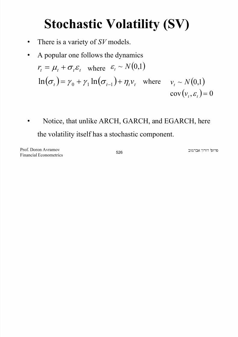
8/22/2019 Avramov Doron Financial Econometrics
http://slidepdf.com/reader/full/avramov-doron-financial-econometrics 526/553
measure volatility.
• It essentially requires no parametric modeling approach.
• Suppose you observe daily observations within a trading
month on the market portfolio.
• RV is the average of the squared daily returns within that
month.
'Prof. Doron Avramov
Financial Econometrics
527
Realized Volatility
• Of course, volatility varies on the monthly frequency but it

8/22/2019 Avramov Doron Financial Econometrics
http://slidepdf.com/reader/full/avramov-doron-financial-econometrics 527/553
is assumed to be constant within the days of that particular
month.
• If you observe intra-day returns (available for large US
firms) then daily RV is the sum of squared of five minute
returns.
'Prof. Doron Avramov
Financial Econometrics
528
Implied Volatility (IV)
• The B&S call Option price is given by

8/22/2019 Avramov Doron Financial Econometrics
http://slidepdf.com/reader/full/avramov-doron-financial-econometrics 528/553
d ln S / K r T
T 1
21
2=+ − +( ) ( )δ σ
σd d T 2 1= − σ
C S,K, ,r,T, Se N d Ke N d - T -rT ( ) = ( ) ( )σ δ δ1 2−
P S,K, ,r,T, Ke N d Se N d -rT - T ( ) = ( ) ( )σ δ δ− − −2 1
• The put Option price is
Where and
'Prof. Doron Avramov
Financial Econometrics
529
Implied Volatility (IV)
• In the traditional option pricing practice one inserts into the
f l ll h i i h k i h ik

8/22/2019 Avramov Doron Financial Econometrics
http://slidepdf.com/reader/full/avramov-doron-financial-econometrics 529/553
formula all the six parameters, i.e., the stock price, the strike
price, the time to expiration, the cc riskfree rate, the cc
dividend yield, and stock return volatility.
• IV is that volatility that if inserted into the B&S formula
would yield the market price of the call or put option.
• As noted earlier, IV in not constant across maturities or across strike prices.
'Prof. Doron Avramov
Financial Econometrics
530
Class Notes in

8/22/2019 Avramov Doron Financial Econometrics
http://slidepdf.com/reader/full/avramov-doron-financial-econometrics 530/553
Financial Econometrics
Stock Return Predictability,Model Selection, and Model
Combination
'Prof. Doron Avramov
Financial Econometrics
531
Return Predictability
• If log returns are IID – there is no way you can deliver better

8/22/2019 Avramov Doron Financial Econometrics
http://slidepdf.com/reader/full/avramov-doron-financial-econometrics 531/553
prediction for stock return than the current mean return.
• That is, if
where is the continuously compounded return and is
the set of information available at time t .
t t r ε µ += where ( )2,0~ σ ε N iid
t
[ ]
[ ] 21
1
|
|
σ
µ
=
=
+
+
t t
t t
I r Var
I r E
t r t I
'Prof. Doron Avramov
Financial Econometrics
532
Return Predictability
• Also note that the variance of a two-period return
i l
1++ t t r r

8/22/2019 Avramov Doron Financial Econometrics
http://slidepdf.com/reader/full/avramov-doron-financial-econometrics 532/553
is equal to
• That is, variance grows linearly with the investment horizon,
while volatility grows in the rate square root.
( ) ( ) ( ) 2
11 2,cov2 σ =++ ++ t t t t r r r Var r Var
'Prof. Doron Avramov
Financial Econometrics
533
Variance Ratio Tests
• However, is it really the case?
P h k l d

8/22/2019 Avramov Doron Financial Econometrics
http://slidepdf.com/reader/full/avramov-doron-financial-econometrics 533/553
• Perhaps stock returns are auto-correlated, or
then:
( ) 0,cov 1 ≠+t t r r
( )( )
( ) ( ) ( )( )t
t t t t
t
t t
r Var r r r Var r Var
r Var r r Var VR
2,cov2
2
1112
+++ ++=+=
( )( ) ( ) ρ σ σ +=+=
+
+ 1,cov
11
1
t t
t t
r r
r r
'Prof. Doron Avramov
Financial Econometrics
534
Variance Ratio Tests
• Test:
0:
0:0
≠
=
ρ
ρ
H
H

8/22/2019 Avramov Doron Financial Econometrics
http://slidepdf.com/reader/full/avramov-doron-financial-econometrics 534/553
• The test statistic is
0:1 ≠ ρ H
( ) ( )1,012 N VRT d
→−
'Prof. Doron Avramov
Financial Econometrics
535
Variance Ratio Tests
• More generally,
8/22/2019 Avramov Doron Financial Econometrics
http://slidepdf.com/reader/full/avramov-doron-financial-econometrics 535/553
no auto correlation
Otherwise H
VR H g
:
1:
1
0 =
( ) s
g
st
g t t t
g g
s
r gVar
r r r Var VR ρ ∑=
++
−+=
+++=
1
1
121K
'Prof. Doron Avramov
Financial Econometrics
536
Variance Ratios
• Test statistic:
12
gd

8/22/2019 Avramov Doron Financial Econometrics
http://slidepdf.com/reader/full/avramov-doron-financial-econometrics 536/553
e.g
( )
−→− ∑
−
+
1
114,01
g
s
d
g g
s
N VRT
2= g
( ) [ ]1,012 N VRT d
→−
3= g
( )
→−920,013 N VRT
d
'Prof. Doron Avramov
Financial Econometrics
537
Predictive Variables
• In the previous specification, we used lagged returns to

8/22/2019 Avramov Doron Financial Econometrics
http://slidepdf.com/reader/full/avramov-doron-financial-econometrics 537/553
forecast future returns or future volatility.
• You can use a bunch of other predictive variables, such as:
• The term spread.
• The default spread.
• Inflation.
• The aggregate dividend yield
'Prof. Doron Avramov
Financial Econometrics
538
Predictive Variables
• The aggregate book-to-market ratio.

8/22/2019 Avramov Doron Financial Econometrics
http://slidepdf.com/reader/full/avramov-doron-financial-econometrics 538/553
• The market volatility.
• The market illiquidity
'Prof. Doron Avramov
Financial Econometrics
539
Predictive Regressions
• To examine whether stock returns are predictable, we can
run a predictive regression.

8/22/2019 Avramov Doron Financial Econometrics
http://slidepdf.com/reader/full/avramov-doron-financial-econometrics 539/553
p g
• This is the regression of future excess log or gross return on
predictive variables.
• It is formulated as:
122111 ++ +++++= t Mt M t t t z b z b z bar ε K
'Prof. Doron Avramov
Financial Econometrics540
Predictive Regressions
• To examine whether either of the macro variables can predict
future returns test whether either of the slope coefficients is

8/22/2019 Avramov Doron Financial Econometrics
http://slidepdf.com/reader/full/avramov-doron-financial-econometrics 540/553
p
different from zero.
• Use the t -statistic or F -statistic for the regression R-squared.
• There is a small sample bias if (i) the predictive variables arehighly persistent, (ii) the contemporaneous correlation
between the predictive regression residual and the innovation
of the predictor is high, or (iii) the sample is small.
'Prof. Doron Avramov
Financial Econometrics541
Long Horizon Predictive
Regressions
zbar ++ ' ε

8/22/2019 Avramov Doron Financial Econometrics
http://slidepdf.com/reader/full/avramov-doron-financial-econometrics 541/553
• The dependent variable is the sum of log excess return over
the investment horizon, which is K periods.
• Since the residuals are auto correlated compute the standard
errors for the slope coefficient accounting for serial
correlation and often for heteroskedasticity.
• For instance you can use the Newey-West correction.
K t t t K t t z bar ++++ ++= ,1,1 ' ε
'Prof. Doron Avramov
Financial Econometrics542
Newey-West Correction
• Rewriting the long horizon regression

8/22/2019 Avramov Doron Financial Econometrics
http://slidepdf.com/reader/full/avramov-doron-financial-econometrics 542/553
[ ][ ]','
,1 ''
,1'
,1
ba
z x
xr
t t
K t t t K t t
=
=+= ++++
β
ε β
'Prof. Doron Avramov
Financial Econometrics
γ
543
Newey-West Correction
• The estimation error of the regression coefficient is

8/22/2019 Avramov Doron Financial Econometrics
http://slidepdf.com/reader/full/avramov-doron-financial-econometrics 543/553
represented by
• where is the Newey-West given by serially correlated
adjusted estimator
( ) S X X Var ˆ'ˆ 1−= β
S ˆ
∑∑ +=−
−= ⋅−
=
T
jt
jt t
K
K j T K
j K
S 1
1ˆ ε ε
'Prof. Doron Avramov
Financial Econometrics
γ
β Var
544
Long Horizon Predictive
RegressionsTradeoff:

8/22/2019 Avramov Doron Financial Econometrics
http://slidepdf.com/reader/full/avramov-doron-financial-econometrics 544/553
•Higher K – better coverage of dependence.
•But we loose degrees of freedom.
•Feasible solution:
3
1
T K ∞
'Prof. Doron Avramov
Financial Econometrics545
Long Horizon Predictive
RegressionsE.g K=1:

8/22/2019 Avramov Doron Financial Econometrics
http://slidepdf.com/reader/full/avramov-doron-financial-econometrics 545/553
•Here we have no serial correlation.
1,0,1 ==−= j j j
∑=
=T
t
t
T
S 1
21ˆ ε
'Prof. Doron Avramov
Financial Econometrics546
Long Horizon Predictive
RegressionsE.g K=2:

8/22/2019 Avramov Doron Financial Econometrics
http://slidepdf.com/reader/full/avramov-doron-financial-econometrics 546/553
2,1,0,1,2 ===−=−= j j j j j
∑∑∑ =−
−=
−
=+ ⋅++⋅=
T
t
t t
T
t
t
T
t
t t
T T T
S 2
1
1
21
1
1
1
2
111
2
1ˆ ε ε ε ε ε
+= ∑ ∑
=
−
=
+
T
t
T
t
t t t
T 1
1
1
1
21ε ε ε
'Prof. Doron Avramov
Financial Econometrics547
In the Presence of
Heteroskedasticity−−
11
111 T T

8/22/2019 Avramov Doron Financial Econometrics
http://slidepdf.com/reader/full/avramov-doron-financial-econometrics 547/553
( )
[ ]∑∑
∑∑
+−
=−−
−=
==
⋅⋅−=
=
1
1
'
1
'
1
'
1ˆ
1
ˆ
11
ˆ
K T
t
jt jt t t
K
K j
t
t t
t
t t
x xT K
j K S
x xT S x xT T Var
ε ε
β
'Prof. Doron Avramov
Financial Econometrics548
Out of Sample Predictability
• There is ample evidence of in-sample predictability, but little
evidence of out-of-sample predictability.

8/22/2019 Avramov Doron Financial Econometrics
http://slidepdf.com/reader/full/avramov-doron-financial-econometrics 548/553
• Consider the two specifications for the stock return evolution
• Which one dominates? If then there is predictability
otherwise, there is no.
:1 M t t t bz ar ε ++= −1
:2 M t t r ε µ +=
1 M
'Prof. Doron Avramov
Financial Econometrics549
Out of Sample Predictability
• One way to test predictability is to compute the out of sample
:2
( )∑ −T
tt r r 2
1ˆ

8/22/2019 Avramov Doron Financial Econometrics
http://slidepdf.com/reader/full/avramov-doron-financial-econometrics 549/553
• Where is the return forecast assuming the presence of
predictability, and is the sample mean (no predictability).
• Can compute the MSE (Mean Square Error) for both models.
( )
( )∑
∑
=
=
−−= T
t
t t
t
t t
OOS
r r
R
1
2
1
1,
2 1
1,t r
t r
'Prof. Doron Avramov
Financial Econometrics550
Model Selection
• When M variable are potential candidates for predicting stock
returns there are linear combinations of predictive models. M 2
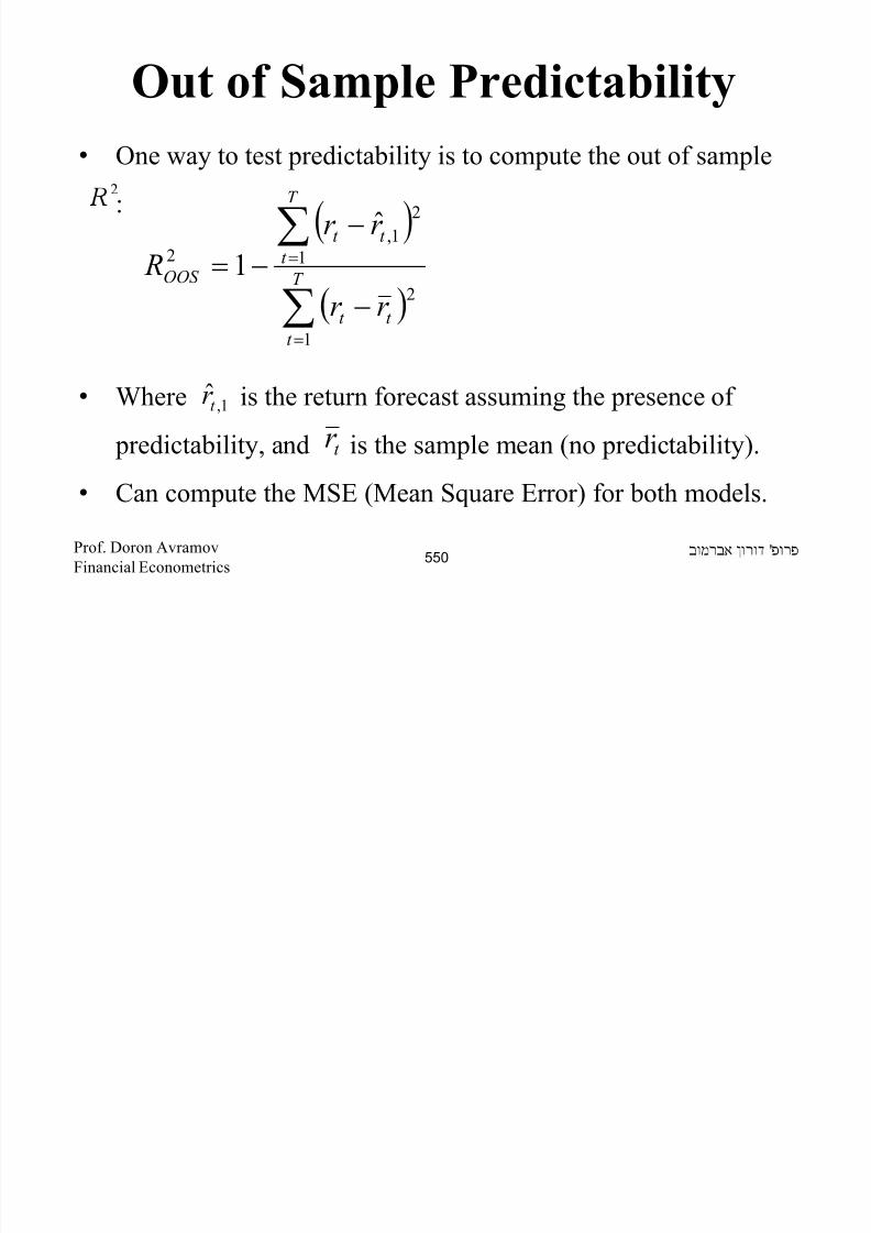
8/22/2019 Avramov Doron Financial Econometrics
http://slidepdf.com/reader/full/avramov-doron-financial-econometrics 550/553
• In the extreme, the model that drops all predictors is the no-
predictability or IID model.
The one that retains all predictors is the all inclusive model.• Which model to use?
• One idea (bad) is to implement model selection criteria.
'Prof. Doron Avramov
Financial Econometrics551
Model Selection Criteria
( ) Lm AIC ln22 −=

8/22/2019 Avramov Doron Financial Econometrics
http://slidepdf.com/reader/full/avramov-doron-financial-econometrics 551/553
where L is the maximized value of the likelihood function.
• Bayesian posterior probability
( ) ( )
( ) ( ) 11
1111
ln2ln
2222
−−−−=−− −−−=
−=
mT m R R
mT T R R
LT m BIC
'Prof. Doron Avramov
Financial Econometrics552
Model Selection
• Notice that all criteria are a combination of goodness of fit
and a penalty factor.

8/22/2019 Avramov Doron Financial Econometrics
http://slidepdf.com/reader/full/avramov-doron-financial-econometrics 552/553
and a penalty factor.
• You choose only one model and disregard all others.
• Model selection criteria have been shown to exhibit very
poor out of sample predictive power.
'Prof. Doron Avramov
Financial Econometrics553
Model Combination
• The other approach is to combine models.
• Bayesian model averaging (BMA) computes posterior

8/22/2019 Avramov Doron Financial Econometrics
http://slidepdf.com/reader/full/avramov-doron-financial-econometrics 553/553
yes ode ve g g ( ) co pu es pos e o
probabilities for each model then it uses the posterior
probabilities as weights to compute the weighted model.
• There are more naive combinations.
• Such combination methods produce quite robust predictors
not only in sample but also out of sample.
'Prof. Doron Avramov
Financial Econometrics554


