33
Affordability Assessment Tool for Federal Water Mandates
Affordability Assessment Tool for Federal Water Mandates

Prepared for
The United States Conference of Mayors
The American Water Works Association
The Water Environment Federation
by
Stratus Consulting, Boulder, Colorado
Copyright 2013, U.S. Conference of Mayors, American Water Works Association, and Water Environment Federation.
All rights reserved.
© Copyright 2013 USCM, AWWA, & WEF 1
Affordability Assessment Tool for Federal Water Mandates
ContentsChapter 1: Assessing the Affordability of Federal Water Mandates provides an overview and critique of EPA’s current approach to assessing affordability and points toward a number of alternative ways to consider the issue.
Chapter 2: Guidance for Developing EPA’s Residential Indicator provides detailed guidance for completing EPA’s preliminary screening analysis for affordability.
Chapter 3: Primary Data Sources for Developing Alternative Measures of Household Affordability describes the data sources that can be used to develop alternative indicators and measures of household affordability for individual communities.
Chapter 4: Guidance for Analyzing Socioeconomic Indicators of Household Affordability for Your Community focuses on the analysis of socioeconomic indicators that can help to provide a more complete picture of economic need within your community.
Chapter 5: Guidance for Developing Alternative Measures of Household Affordability provides guidance for developing specific household affordability metrics.
Chapter 6: Guidance for Assessing Utility Financial Capability: EPA’s Secondary Screening Analysis and Alternative Measures provides specific guidance for analyzing utility financial capability, including EPA-suggested metrics and alternative approaches.
Bibliography Workbook 1: EPA Guidance for Estimating the RI Workbook 2: Accessing ACS Data at the Community, National, and Census-Tract Levels Workbook 3: Socioeconomic Indicators Workbook 4: Developing Alternative Metrics Workbook 5: EPA’s Secondary Screening Analysis
Figures4-1 MHI by Census tract, 2011, developed using American Fact Finder website 4-2 MHI by Census tract, 2011 4-3 Kansas City MHI, 2005–2011, adjusted to 2011 dollars using CPI 4-4 Income distribution in Atlanta, Georgia and the United States 4-5 Income distribution in Atlanta, Georgia, elderly households and citywide 4-6 Atlanta, Georgia income distribution, renter- and owner-occupied households 5-1 Average annual wastewater bill as a percentage of Census tract MHI, Philadelphia, Pennsylvania 5-2 Estimated average wastewater and combined water and wastewater bills as a percentage of household income,
Sacramento, California

2 © Copyright 2013 USCM, AWWA, & WEF
Affordability Assessment Tool for Federal Water Mandates
Tables2-1 Typical data sources for calculating EPA’s CPH 4-1 MHI by household type, Kansas City, Kansas 4-2 Household income quintile upper limits, Atlanta, Georgia and the United States 5-1 Estimated average wastewater bill as percentage of MHI by income category, Butte, Montana 5-2 Estimated average wastewater bill as a percentage of federal poverty threshold incomes 5-3 Average annual total household water and wastewater bill as a percentage of MHI
by household type, Kansas City6-1 Permittee FCI benchmarks and their ratings: EPA Guidance
List of Acronyms and AbbreviationsACCRA American Chamber of Commerce Research Association ACS American Community Survey AFF American Fact Finder AWWA American Water Works Association BLS Bureau of Labor Statistics CES Consumer Expenditure Survey COLI Cost of Living Index CSO Combined Sewer Overflow CPH cost per household CPI consumer price index CWA Clean Water Act EJ environmental justice EPA U.S. Environmental Protection Agency FCI Financial Capability Indicators FMPV fair market property value GIS geographic information systems GO general obligation IPMS Integrated Public Use Microdata Series IPPP Integrated Planning and Permit Policy LAUS Local Area Unemployment Statistics MHI median household income MOE margin of error O&M operations and maintenance PUMA Public Use Microdata Area RI Residential Indicator SDWA Safe Drinking Water Act SPM Supplemental Poverty Measure USCM U.S. Conference of Mayors WEF Water Environment Federation WQS water quality standards WWT wastewater

© Copyright 2013 USCM, AWWA, & WEF 3
Affordability Assessment Tool for Federal Water Mandates
Chapter 1
Assessing the Affordability of Federal Water MandatesCommunities and the water agencies that serve them have limited resources, so the investments they make need to address the most important risks to public health and the environment and deliver maximum benefits at a cost that is affordable. This Water Mandates Affordability Assessment Tool (Assessment Tool) is the result of a collaborative ef-fort by the United States Conference of Mayors (USCM), the American Water Works Association (AWWA), and the Water Environment Federation (WEF). Its purpose is to raise issues, provoke discussion and provide alternative ways to view the affordability of federal water mandates in any given community. It does not represent the official policy of the sponsoring organizations or their members.
This chapter summarizes the U.S. Environmental Protec-tion Agency’s (EPA’s) methods for analyzing the afford-ability of federal mandates stemming from the Clean Water Act (CWA) and Safe Drinking Water Act (SDWA). It describes the Agency’s current policies, offers a critique, and identifies a number of alternatives that might be more suitable for analyzing the affordability of water and waste-water mandates on American communities. Finally, this chapter notes the importance of weighing benefits as well as costs when considering federal water mandates. As the reader will note, the term “water” is used throughout the Assessment Tool to mean drinking water, wastewater, and stormwater, unless otherwise noted.
BackgroundInvestment to meet federal water and wastewater re-quirements can impose significant financial hardships on households, businesses, and the broader communities in which they are located. When communities face large—and sometimes multiple—federal water mandates, the combined impact of the required expenditures can be extremely expensive for everyone in that community who pays a water or wastewater bill (most consumers get one combined bill for water and wastewater services). For the utility, the cumulative suite of required investments not
only strains fiscal capacity but may also displace other im-portant investments, including critical but nonmandatory capital improvement and infrastructure renewal projects. For the greater community, mandatory investments may also squeeze out other important priorities, such as social safety net programs and economic development efforts. For the residents and businesses in affected communities, the capital and operating expenses associated with federal mandates are often reflected in water and wastewater bills that must grow faster than household incomes and the general rate of inflation. Very significant affordability challenges are often created, particularly for lower-income households.
With the intention of providing a mechanism for relieving undue economic stress in the face of wastewater-related mandates, EPA has developed “affordability” criteria to indicate when such mandates would cause substantial and widespread economic distress in the community. In the case of undue economic stress caused by wastewater re-quirements, the Agency might be willing to exercise some flexibility in the mandate by allowing a longer timeframe to achieve compliance or by relaxing compliance standards. The affordability of drinking water requirements is han-dled differently and can—at least in theory and case-by-case—affect the kind of technology that must be deployed in some small communities.
If EPA affordability criteria functioned properly, the economic hardship imposed on lower-income households might be alleviated in many communities. Unfortunately, there are several critical limitations to how EPA defines affordability and applies its assessment criteria. This is due in part to EPA’s reliance on metrics such as median household income (MHI), which is highly misleading as an indicator of a community’s ability to pay. As a result, reg-ulatory relief is not provided in many communities where substantial and widespread economic hardships are indeed being created.

4 © Copyright 2013 USCM, AWWA, & WEF
Affordability Assessment Tool for Federal Water Mandates
EPA’s Two-level Affordability Screening Analysis for Wastewater and Combined Sewer Overflow (CSO) ControlsIn 1995, EPA published its first set of affordability-related guidelines: The Interim Economic Guidance for Water Quality Standards. The 1995 Guidance contains a detailed discussion of the analyses a municipality should undertake to evaluate the economic impact of complying with water quality standards (WQS) under the CWA. In 1997, EPA published Guidance for Financial Capability Assessment and Schedule Development using a nearly identical approach to assess whether an extended compliance schedule might be granted to a community facing afford-ability problems. The analyses put forth in these guidance documents are divided into two parts:
1. The preliminary screen examines affordability using a factor called the Residential Indicator (RI). The RI weighs the average per household cost of wastewater bills relative to median household income in the service area. Ultimately, an RI of 2% or greater is deemed to signal a “large economic impact” on residents, meaning that the community is likely to experience economic hardship in complying with federal water quality standards.
2. A secondary screen examines metrics related to the financial capability of the impacted community. This screen applies a Financial Capability Indicator (FCI) reflecting the average of six economic indicators. Those indicators include the community’s bond rating, its net debt, its MHI, the local unemployment rate, the service area’s property tax burden, and its property tax collection rate. Each indicator is assigned a score of 1 to 3, based on EPA-established benchmarks. Lower FCI scores imply weaker economic conditions and thus an increased likeli-hood the mandate would cause substantial and widespread economic impact on the community or service area.
The results of the RI and the FCI are ultimately combined into an overall rating based on EPA’s Financial Capability Matrix. This rating is intended to demonstrate the overall level of financial burden imposed on a community by com-pliance with CWA mandates.
EPA’s Assessment of Affordability for Drinking Water Regulations Whereas EPA’s consideration of affordability for wastewa-ter and CSO compliance is aimed at assessing an individual community’s ability to comply with regulatory mandates and schedules, EPA’s consideration of affordability in the context of potable water supply is limited to assessing the national-level affordability of regulatory options for small communities. EPA does not consider the affordability of
drinking water requirements in any manner that pertains to individual utilities (even small ones), or to the category of medium and large utilities.
EPA has stated that it would consider a National Primary Drinking Water Regulation to be unaffordable to small communities (those with populations under 10,000) if the standard would result in a household drinking water bill in excess of 2.5% of the national MHI in such communities. In this context, MHI is evaluated based on all small commu-nity water systems collectively (i.e., MHI is not considered for any individual utility, but for all small utilities lumped together). To date, EPA has never determined that a drink-ing water regulation is unaffordable for small systems. If EPA were to make such a finding, it would be required to identify technologies for small systems that might not result in meeting a particular drinking water standard but are found to protect public health. Then, on a case-by-case basis, states may approve the use of such affordable small system technologies (called a variance) or approve an extended deadline for compliance (called an exemption). States cannot approve both a variance and an exemption for the same standard in the same community. Variances are subject to review and approval by EPA. States have allowed very few variances and exemptions because they can be difficult and expensive to issue.
EPA’s stated view on potable water—that it is affordable if it costs less than 2.5% of small community MHI—influ-ences the perceived affordability of combined water and wastewater bills. Specifically, it is commonly inferred that EPA would consider a combined annual water and waste-water bill of less than 4.5% of MHI to be affordable (2.5% for water, plus 2% for wastewater services and CSO controls).
Limitations of EPA’s Preliminary Screening ApproachA central issue in assessing affordability of federal water mandates is the reasonableness of community-wide MHI as a primary yardstick. MHI can be a highly misleading indi-cator of a community’s ability to pay for several reasons.
• MHI is a poor indicator of economic distress and bears little relationship to poverty or other measures of econom-ic need within a community. For example, consider an analysis of MHI and poverty data for the 100 largest cities in the United States. It shows that for 21 cities identified as having an MHI within $3,000 of the 2010 national MHI ($50,046), there is no discernible relationship between MHI and the incidence of poverty. Statistical analysis confirms that the correlation between MHI and poverty among these cities is not meaningful, with a correlation coefficient (r) of 0.024. Indeed, within these 21 cities, the poverty rate ranges from a low of 14.1% to a high of 23.3%.

© Copyright 2013 USCM, AWWA, & WEF 5
Affordability Assessment Tool for Federal Water Mandates
• MHI does not capture impacts across diverse populations. In many cities, income levels are not clustered around the median, but are spread over a wide income range or concentrated at either end of the income spectrum. This tendency for the income distribution to spread away from the middle has been increasing and may well continue to increase in the future, making MHI an even less mean-ingful metric. In addition, income distribution and other economic measures can vary widely across different dis-tricts and neighborhoods within a city. Thus, the economic hardship associated with increasing water and wastewater bills can be concentrated in a few lower-income neighbor-hoods. This will compound the economic hardship within the community and may raise issues of environmental justice (EJ). These impacts are not captured with the use of service area MHI as a sole indicator.
• MHI provides a “snapshot” that does not account for the historical and future trends of a community’s economic, demographic, and/or social conditions. This is particularly relevant in areas that may be experiencing economic declines or population losses (which will result in the costs of water and wastewater programs being spread across fewer residents). Without consideration of these and other economic and demographic trends, the affordability determination will overestimate the ability of residents to tolerate rate increases over time.
• MHI does not capture impacts to landlords and public housing agencies. Many renters do not receive water bills because water and wastewater service is included in the cost of rent. The same is true of many residents in public housing. In cities with a high percentage of renters and/or public housing residents, use of MHI and RI does not capture impacts to landlords and public housing agencies, which must often absorb the cost of increased water and wastewater bills. In many cases, higher water bills mean that public housing authorities will be required to reduce the number of needy renters they serve, unless there can be offsetting increases in public housing budgets.
• The RI does not fully capture household economic burdens. Economic burdens are commonly measured by comparing the costs of particular necessities to available household income. The RI is such a measure in that it is used to evaluate the economic burden from water bills by comparing those bills to MHI. However, there can be situations where the economic burdens in a community are substantially different from those typically associated with its RI. For example, a community may experience unusually high costs of basic necessities or may have a distribution of household income that differs significantly from that in most communities. In these cases, the standard application
of EPA’s RI would be insufficient on its own to distinguish between higher and lower levels of economic impact.
Alternative Household Affordability Metrics: Moving Beyond EPA’s Criteria Given the limitations of the RI, and in particular the use of MHI as a primary indicator of household affordability, it is important to consider the use of alternative metrics to gauge the affordability of federal water, wastewater, and stormwater-related mandates. For example, impacts on customer bills can be assessed as follows:
• Across the income distribution. Given the relatively large percentage of households in the lower portions of the in-come distribution in many cities, it is important to examine the effect of rising water bills across the entire income dis-tribution—and especially at the lower end—rather than simply at the median. For example, a key indicator could include the analysis of average water and wastewater bills as a percentage of the household income for each income quintile. Table 1-1 demonstrates that this percentage would be much higher for lower income quintiles in Atlanta com-pared to national levels (e.g., the income level that defines the upper end of the lowest quintile—lowest 20% of income earners—in Atlanta is $12,294; this compares to $20,585 nationally).
Table 1-1 Household Income Quintile Upper Limits in Atlanta, Georgia, and the United States (2011$)
Atlanta, Ga. United States
Lowest quintile 12,294 20,585
Second quintile 31,873 39,466
Third quintile 59,043 63,001
Fourth quintile 104,233 101,685
Lower limit of top 5% 246,335 187,087
Source: U.S. Census Bureau American Community Survey, 2012.
EPA’s “Guidance for Preparing Economic Analyses” (240-R-00-003) recognizes the legitimacy of assessing impacts to all households across the income distribution, though EPA has not provided information on how such analyses have been conducted in the past or how they’ve been used in enforcement actions.
• Across household types. Average water and wastewa-ter bills can be examined as a percentage of income for potentially vulnerable populations (e.g., renters and elderly households).
6 © Copyright 2013 USCM, AWWA, & WEF
Affordability Assessment Tool for Federal Water Mandates
• Across neighborhoods or similar geographic units, such as Census tracts, or Public Use Microdata Areas (PUMAs). Poverty rates and households located in poverty areas can be considered to identify portions of communities that are economically at risk. Alternative measures of poverty, such as the Supplemental Poverty Measure (SPM) recently de-veloped by the U.S. Census Bureau , can be especially use-ful in this respect. The analysis could capture affordability issues in particular parts of a community or service area that may be masked when looking at the area as a whole.
Other indicators of economic need and widespread impacts can also be considered for the community or parts of the community2. These might include:
• The unemployment rate.
• The percentage of households receiving public assistance such as food stamps or living below the poverty level.
• The percentage of households meeting Home Energy Assistance Program requirements.
• The percentage of customers eligible for water affordability programs.
• The percentage of households paying high housing costs—for example the percentage of households with housing costs in excess of 35% of income.
• Other household cost burdens such as nondiscretionary spending as a percentage of household income for house-holds within each income quintile (Rubin 2003).
EPA’s Secondary Screening Analysis: Limitations and Alternative Indicators Just as the RI falls short of its intended purpose, so too does the FCI. The FCI that makes up EPA’s secondary screening analysis does not adequately reflect a community’s ability to finance investments associated with federal water mandates. This measure fails to fully capture financial capability because:
• EPA uses property tax revenues as a percentage of full market property value (FMPV) as its sole measure of local tax effort. Focusing solely on property taxes—while ignor-ing income, sales, business taxes, and user fees typically charged for city services—inevitably understates the tax
effort in cities that rely on multiple forms of taxation. As an alternative, EPA should allow municipalities to use total local tax and fee revenues as a percentage of gross taxable resources. This would provide a better measure of the extent to which a municipality is already using the full range of its taxable resources.
• The secondary screening analysis includes measures of local MHI and unemployment levels compared to the national average. By focusing on how these measures compare with national levels, EPA fails to acknowledge the profound impact of the absolute levels themselves. For example, if the national unemployment rate is 9%, a community with an unemployment rate of 10% is consid-ered by EPA as having only a “mid-range” unemployment problem. In fact, a community with a 10% unemployment rate is all-but-certain to be experiencing significant dis-tress, regardless of the national average.
o In addition to supplemental measures for MHI (as previously described), EPA should consider a metric that compares a municipality’s current unemployment rate with the long-term state and national average (the national average was 5.8% between 1991 and 2010). Use of the long-term state and national averages as a benchmark would provide a more insightful socioeco-nomic indicator than a single current number. A com-munity’s long-term unemployment rate (for example, the share of the labor force continuously unemployed for one-half year or more) could also be evaluated.
o In addition to broadening the range of labor market indicators it considers in assessing local financial ca-pabilities, EPA should consider other measures of local economic distress, such as foreclosure rates. At the national level, foreclosure rates rose from 5.8 per 1,000 households in 2006 to 22.2 per 1,000 in 2010 (Office of the State Comptroller, 2011). In many communities, high foreclosure rates have had a significant impact on the financial condition of local governments and their ability to finance capital improvements.
• The FCI does not take into account the recent deterio-ration of many local governments’ ability to finance major capital improvements, as evidenced in municipal capital markets. EPA should consider adding a measure of local government revenue growth or decline to the FCI matrix,
The SPM includes changes in the measure of available household resources (e.g., using after-tax income instead of pretax income and taking into account income received through food stamps and other forms of public assistance) and also recognizes some nondiscretionary expenses that such households bear. The SPM also adjusts for different housing status (e.g., renters versus owners). Additional details can be found in the U.S. Census Bureau’s Supplemental Poverty Measure (2011a).
2 EPA’s 1995 Interim Economic Guidance for Water Quality Standards provides a good list of these indicators, and also includes economic losses, impacts on property values, decreases in tax revenues, and potential for future job losses, among others.

© Copyright 2013 USCM, AWWA, & WEF 7
Affordability Assessment Tool for Federal Water Mandates
with a decline in real revenues over some period taken as a sign of weakened financial capacity.
• EPA’s methodology for assessing municipalities’ financial capabilities takes into account formal debt burden, but it does not consider what for many cities is an even greater li-ability: unfunded pension and health care commitments to retirees. These are generally not reflected in formal debt.
• Community or utility revenues are not considered in the secondary screening analysis. This creates a signifi-cant weakness, especially in areas that are experiencing economic difficulties, delinquency in water and wastewater payments, declining water usage, shrinking revenues, or a growing number of older customers on fixed or declining incomes. EPA should consider the addition of more appro-priate measures of revenue collection, such as current de-linquency rates, the agency’s ability to enforce collection, and its likelihood of recovering these costs.
• EPA’s secondary screening analysis does not take into account the fact that many communities have a legal debt ceiling. Debt limitations have the potential to severely limit a community’s ability to finance unfunded mandates absent an extended schedule.
• Finally, EPA does not consider the longer-term needs facing many municipalities for reinvestment and renewal of water and wastewater infrastructure due to the current system’s age and condition. As documented by AWWA’s Buried No Longer report (covering buried drinking water infrastructure only), these needs add up to at least $1 tril-lion over the next 25 years. Wastewater needs are at least as great, not counting CSO costs. The need for this invest-ment is real and urgent.
Weighing the Benefits of Additional Mandate-Driven ExpendituresFederal Clean Water Act and the Safe Drinking Water Act mandates are intended to provide better public health pro-tection, water quality enhancements, and other benefits. However, not all drinking water and wastewater mandates are the same. Some provide greater benefits than others, or provide benefits sooner than others, or generate benefits to different groups of people or ecosystems.
When communities face expensive water mandates and associated deadlines, the impact of the required expen-ditures can be extremely difficult for all who pay water bills, but particularly for those with lower incomes. In such communities, the expected benefits of the mandate should be carefully weighed against:
• Compliance deadlines (which might be amended)
• Permit limits (which might be adjusted)
• Required compliance technologies and strategies (some of which are more expensive than others)
• Other factors that influence the magnitude and timing of required investments
When the costs of meeting a regulatory mandate are high, the affordability implications and the benefit of the activity should each be evaluated in concert with the other. The most important questions include:
1. Are the added benefits of more rapid and/or stringent mandates warranted given the added costs and adverse impacts on affordability, when compared to less stringent, perhaps less expensive alternatives?
2. Are projects with lower public health or environmental benefits driving out projects that might be of greater value to the community or the nation?
3. Are the households that will realize most of the benefits different than those who will bear most of the costs?
4. Are those bearing the greatest burden economically disadvantaged and thus worthy of environmental justice consideration?
EPA’s proposed Integrated Planning and Permit Policy (IPPP) provides one potential avenue by which the costs and benefits of all federal water mandates could be ad-dressed. The IPPP process could be used to set priorities, make adjustments in requirements, and set reasonable timetables. Such adjustments would help ensure that local resources are used to secure the greatest public health and environmental benefits at an affordable cost. Moving the IPPP process forward as suggested offers important potential advantages:
• Comparing the environmental, social, and financial bene-fits of all water-related obligations would allow municipali-ties to develop priorities that reflect the totality of trade-offs and commitments facing the community.
• Considering all water-related obligations together, and assessing financial capability in light of total water-related obligations, would focus local resources where the com-munity will get the greatest total environmental, public health, and other benefits.
It should be noted that EPA does not include drinking wa-ter mandates in the Integrated Municipal Stormwater and

8 © Copyright 2013 USCM, AWWA, & WEF
Affordability Assessment Tool for Federal Water Mandates
Wastewater Planning process, even though drinking water investments must be carried on the same customer bill as investments needed to comply with wastewater and CSO mandates. The USCM, AWWA, and WEF have recommended that EPA include consideration of drinking water invest-ments in the Integrated Planning and Permit Program. The program should also consider necessary but nonmandatory investments in the ongoing rehabilitation of water and wastewater infrastructure.
© Copyright 2013 USCM, AWWA, & WEF 9
Affordability Assessment Tool for Federal Water Mandates
Chapter 2
Guidance for Developing EPA’s Residential IndicatorThis chapter provides an overview of the methods outlined in EPA’s 1997 Guidance for Financial Capability Assessment and Schedule Development ( U.S. EPA, 1997), which EPA uses for completing the preliminary screening analysis (i.e., calculating the RI). More specific instruc-tions and worksheets developed by EPA for this purpose are included in this Assessment Tool as Workbook 1, an Excel spreadsheet.
EPA’s RI is intended to provide a measure of the financial impact of current and proposed wastewater treatment (WWT) and CSO controls on residential users. The calculation of the RI involves the following steps:
• Determine the average annual cost per household (CPH) associated with WWT- and CSO-related programs and services in a given community. CPH is based on the total costs for these programs, the percentage of wastewater flow attributable to residential users, and the number of households in the service area, as further explained below.
• Determine the MHI for the service-area based on data from the U.S. Census Bureau.
• Divide the CPH by the service area MHI to calculate the RI.
• Compare the RI to financial impact ranges established by EPA to determine whether unfunded mandates will produce a possible high, mid-range, or low financial impact on residential users.
It is important to note that although EPA’s 1997 Guidance was developed within the context WWT and CSO controls, this Assessment Tool is focused on the affordability of both water supply and WWT (including CSO and stormwater) programs. For comparison purposes, water and wastewater utilities can calculate the average annual CPH for both types of services using the methodology outlined below.
Step 1: Develop the CPH Estimate
In its 1997 Guidance, EPA outlines the following steps for determining the average annual CPH of existing and pro-posed WWT and CSO control costs:
• Determine total WWT and CSO (and stormwater) costs by adding together the current costs for existing WWT opera-tions and projected costs for any proposed controls.
o Current WWT costs are defined as “current annual wastewater operating and maintenance (O&M) expens-es (excluding depreciation) plus current annual debt service (principal and interest)” (1997 Guidance, p. 12).
o EPA Guidance states that O&M expenses and debt service costs should also be estimated for all proposed projects and adjusted to current year dollars (i.e., deflated) using the average annual national Consumer Price Index (CPI) inflation rate for the last five years. Workbook 1 includes specific instructions for applying the CPI and determining annualized debt service costs.
• Calculate the residential share of the total WWT and CSO costs.
o The residential share of total costs is computed by multiplying the percent of total wastewater flow (in-cluding infiltration and inflow) attributable to residen-tial users by the total costs.
• Calculate the CPH by dividing the residential share of the total WWT and CSO costs by the number of households within the service area.
The sources of data necessary for calculating CPH will vary somewhat by utility/municipality. Table 2-1 provides a summary of typical data sources.
Step 2: Determine Service-area MHI The second step in developing the RI is to determine MHI for your service area (or general service area boundaries if the service area does not exactly follow Census-designated areas). In its 1997 Guidance, EPA recommends using the MHI from the latest census year and adjusting it to current year dollars using the average CPI inflation rate. However, the Decennial Census no longer includes MHI as a statistic. MHI is reported annually as part of the U.S. Census Bureau American Community Survey (ACS), which can be accessed via the American FactFinder (AFF) website at factfinder.

10 © Copyright 2013 USCM, AWWA, & WEF
Affordability Assessment Tool for Federal Water Mandates
census.gov/faces/nav/jsf/pages/index.xhtml. Additional detail and instructions for accessing ACS data are included in chapter 5, as well as in Workbooks 2, 3, and 4 that are included with this Assessment Tool.
EPA’s 1997 Guidance also states that if the service area includes more than one jurisdiction, a weighted MHI should be developed based on the number of households within each area. In addition, if MHI is unavailable for a specific service area or jurisdiction, EPA suggests that the surrounding county’s MHI may be sufficient.
Step 3: Calculate and Analyze the RITo calculate the RI, the annual CPH is divided by the MHI of the service area. The RI indicator is then compared to financial impact ranges established by EPA to determine whether unfunded mandates will produce a possible high,
mid-range, or low financial impact on residential users. In the context of wastewater, CSO, and stormwater controls, the RI is categorized as low if it is less than 1%, mid-range if it is between 1% and 2%, and high if it is greater than 2%. For drinking water, an RI of greater than 2.5% is consid-ered to represent a high financial impact.
In its 1997 Guidance, EPA suggests that if the wastewater RI is classified as “mid-range” or “high”, then the communi-ty should perform a secondary screening analysis (i.e., cal-culate the FCI) to assess the utility’s financial capability to afford additional programs. Results from the preliminary and secondary screening analyses are ultimately combined into EPA’s Financial Capability Matrix to determine wheth-er a community should be granted a longer compliance schedule for meeting regulatory obligations, or provided another form of relief.
Table 2-1 Typical data sources for calculating EPA’s Cost per Household
Component of CPH Data source
Current annual WWT, CSO, or stormwater costs Utility/municipality financial reports (in some states these are available from central records kept by the state auditor or other state offices)
Projected annual WWT, CSO, or stormwater costs Utility/municipal planning documents
CPI Bureau of Labor Statistics (USDOL BLS, 2012)
Percent of total wastewater flow attributable to residential users Utility billing data
Number of households in service area Utility/municipal planning documents, U.S. Census Bureau ACS single-year estimates for most recent yeara
aU.S. Census Bureau ACS data can be used if service area boundaries follow Census divisions (e.g., county, city, Census tracts, metropolitan statistical areas). Chapter 5 provides additional detail on ACS data.

© Copyright 2013 USCM, AWWA, & WEF 11
Affordability Assessment Tool for Federal Water Mandates
Chapter 3
Primary Data Sources for Developing Alternative Measures of Household AffordabilityThis chapter provides an overview of the data sources that can be used to develop the metrics outlined in the subse-quent chapters (4 and 5), including:
1. U.S. Census Bureau American Community Survey (ACS, the primary data source)
2. U.S. Census Bureau Integrated Public Use Microdata Series (IPUMS)
3. Additional national, state, and local sources.
Use these data sources to develop alternative measures of household affordability (i.e., beyond EPA’s RI). Such alter-native measures include a series of socioeconomic indica-tors, such as income distribution and poverty rates within a community, as well as specific affordability metrics for different household types.
Workbooks 2 and 3 provide more information and step-by-step instructions for accessing and analyzing this data.
U.S. Census Bureau ACSThe U.S. Census Bureau ACS serves as the primary source of data used to develop the affordability measures rec-ommend in this Assessment Tool. The ACS is a household survey conducted by the U.S. Census Bureau with a current annual sample size of approximately 3.5 million house-holds. The ACS replaced sample (long-form) data from the Census and is now the only source of data on income, poverty status, education, employment, and most housing characteristics. ACS estimates are released annually (for geographic areas with a population of 65,000 or more), as a three-year average (for geographic areas with a population of 20,000 or more), and as a five-year average (for all geog-raphies, down to the Census Block Group level). The ACS is considered the most reliable source of detailed socioeco-nomic data currently available, and is the only source of data available for small geographies.
ACS datasets can be used to access socioeconomic data that will allow better examination of economic need within a community, including:
• Income levels and income distribution
• Poverty rates
• Unemployment rates
• Households receiving public assistance
• Some information on housing costs and housing burden
ACS data are also used in this Assessment Tool to develop specific affordability metrics, such as comparing average household water and wastewater bills to the MHI for each income quintile, and examining EPA’s RI at the census tract level to identify potentially vulnerable communities.
ACS data are available on the U.S. Census Bureau’s American FactFinder website. One-year estimates are typically released for the previous year every September, three-year estimates in October, and five-year estimates in December. As of December 1, 2012, the U.S. Census Bureau has released one-year estimates for 2011 and three-year estimates for 2009-2011. Five-year average estimates are scheduled for release on December 6, 2012.
Throughout this Assessment Tool, USCM, AWWA, and WEF recommend using the ACS to collect socioeconomic data at the city (or service area) level (i.e., using single-year or three-year average ACS estimates), as well as at smaller geographic scales (e.g., at the Census tract level, using five-year average ACS estimates). Analysis of these data on a smaller-scale (such as a Census tract or neighborhood) can help to identify vulnerable populations and assess potential EJ concerns.
Workbooks 2 and 3 provide additional information and step-by-step instructions for accessing, reporting, and map-ping both one-year and five-year average ACS estimates. This includes guidance on navigating the AFF website, specific source tables for socioeconomic data, and select-ing the correct geographic area (e.g., place within a state, county, metropolitan service area) for your service area.
12 © Copyright 2013 USCM, AWWA, & WEF
Affordability Assessment Tool for Federal Water Mandates
U.S. Census Bureau IPUMS In addition to ACS data, more in-depth analyses can be performed using the U.S. Census Bureau’s IPUMS. IPUMS can be used to analyze socioeconomic characteristics across different types of households (e.g., renter-occupied versus owner-occupied households, multi-family versus single-family) or to run queries or cross tabs at the city- or PUMA-level. PUMAs are statistical geographic areas that have been defined for the tabulation and dissemination of IPUMS data. PUMAs are made up of clusters of Census tracts and have a population of at least 100,000.
IPUMS consists of more than 50 high-precision samples of the American population drawn from 15 federal Censuses and 2000–2010 ACS data. IPUMS is composed of microdata, meaning that each record is a person. In most samples, persons are organized into households, making it possible to study the characteristics of people in the context of their families or other co-residents. Because IPUMS uses census results from individuals, it is possible to drill down into much deeper detail than possible with ACS summaries. For example, IPUMS data can be used to determine the percentage of people at certain income levels in differ-ent areas of a city or community (e.g., the percentage of residents with incomes greater than the 2% affordability threshold income).
The use of PUMS data presents several obstacles for water and wastewater utilities. Most importantly, because the data are individuals and not tables, researchers must use advanced statistical packages (such as SPSS, SAS, S-plus, or R software programs) to analyze the millions of records in the database. In addition, the large size of the PUMAs (100,000 people) is a potential problem for smaller cities. Further, because PUMAs must include 100,000 people, some PUMA boundaries are arbitrary and do not always follow political or common geographical delineations.
For these reasons, this Assessment Tool does not provide in-depth detail on how to access and analyze IPUMS data. However, the use of these data by water and wastewater
utilities may be performed in-house or by consultants with relevant knowledge. More information on IPUMS can be found at www.census.gov/acs/www/data_documentation/public_use_microdata_sample/.
Throughout the remainder of this Assessment Tool, places where IPUMS data would serve to augment household affordability assessments are noted; however, the As-sessment Tool and analyses focus on more accessible and user-friendly data sources.
Supplemental Data SourcesIn addition to U.S. Census Bureau surveys, state and local data sources can also provide a wealth of relevant infor-mation. The availability of these sources will vary across utilities/municipalities and may include information from states’ labor departments (e.g., particularly for unemploy-ment data), economic development and local government agencies, and other local agencies and organizations.
Another source of supplemental data may include datasets that provide information on nondiscretionary spending and housing costs within a city compared to the national average, or some other benchmark. This information can help to demonstrate the burden that these costs place on different types of households and can provide insight into the potential effects of water and wastewater rate increases. For example, in larger communities where the cost of living is high and incomes are commensurate with the national average, the American Chamber of Commerce Research Association (ACCRA) Cost of Living Index (COLI) database might serve as an important measure of existing household burdens. The ACCRA COLI database provides a measure of differences in the cost of living among urban areas in the United States relative to price levels for con-sumer goods and services in participating areas. Data from the BLS Consumer Expenditure Survey (CES) can also be used to assess economic burdens within different types of communities, including both urban and rural communities. More information on the ACCRA COLI is available at www.coli.org/.
© Copyright 2013 USCM, AWWA, & WEF 13
Affordability Assessment Tool for Federal Water Mandates
Chapter 4
Guidance for Analyzing Socioeconomic Indicators of Household Affordability for Your CommunityThere is no single piece of information that can definitively indicate whether a community is at risk of being unable to afford increased water and wastewater costs. However, relevant socioeconomic indicators can help to provide a more complete picture of a community’s economic and social characteristics (and thus, its ability to afford rate increases associated with unfunded mandates). This Assessment Tool (and associated templates) focuses on the following indicators of social and economic need1:
• Income levels
• Income distribution
• Poverty rates
• Household economic burdens and nondiscretionary spending
• Supplemental indicators, including households receiv-ing public assistance and unemployment rates within a community.
The following sections provide an overview of the socio-economic indicators described above, as well as general guidance for accessing and analyzing specific socioeconom-ic data. We do not propose specific affordability thresholds for these indicators, rather, they are intended to provide context and to help “build the case” for why a community may merit additional consideration for regulatory relief.
Throughout this Assessment Tool, graphs and tables for specific indicators are presented, drawing upon data from various U.S. cities as examples. Workbook 2, “Assessing American Community Survey Data at the Community,
National, and Census-Tract Levels,” includes step-by-step instructions for accessing the ACS data necessary for analyzing each indicator. Workbook 3 provides templates for developing specific analyses for your community2.
Income Levels
Although not useful as a sole indicator of household afford-ability, MHI data will serve as an important component of your household affordability assessment. In addition to providing an indication of economic need, MHI data will be used to develop specific affordability measures (e.g., evaluating water and wastewater rates as a percentage of MHI by Census tract or within each income quintile).
The first order of business is to document MHI for your community for the most recent year available, compared to the national MHI for the same year (in 2011, the MHI in the United States was $50,502). Citywide or service area-wide income data are easily obtained via American FactFinder (AFF) using the ACS single-year, three-year average, or five-year average dataset, depending on the size of your community. See Workbooks 2 and 3 with this Assessment Tool.
To identify specific areas in your community with high concentrations of low-income households, MHI data should also be analyzed at the Census tract level. These data will be based on five-year average estimates from the ACS because single-year data are not available at this smaller geographic scale (5-year average estimates are available for all geographies). These data should be downloaded via AFF into Excel spreadsheets for further analysis.
1 There are other indicators that localities and utilities may want to consider, particularly those listed in the EPA 1995 Interim Eco-nomic Guidance for Water Quality Standards Workbook as part of the widespread economic impact analysis; these indicators include: losses to local economy; increases in unemployment; impacts on property values or community development potential; decreases in tax revenues; loss of future jobs or personal income. See this EPA guidance for a complete list.
2 ACS estimates are released annually (for geographic areas with a population of 65,000 or more), as a three-year average (for geograph-ic areas with a population of 20,000 or more), and as a five-year average (for all geographies, down to the Census Block Group level).
14 © Copyright 2013 USCM, AWWA, & WEF
Affordability Assessment Tool for Federal Water Mandates
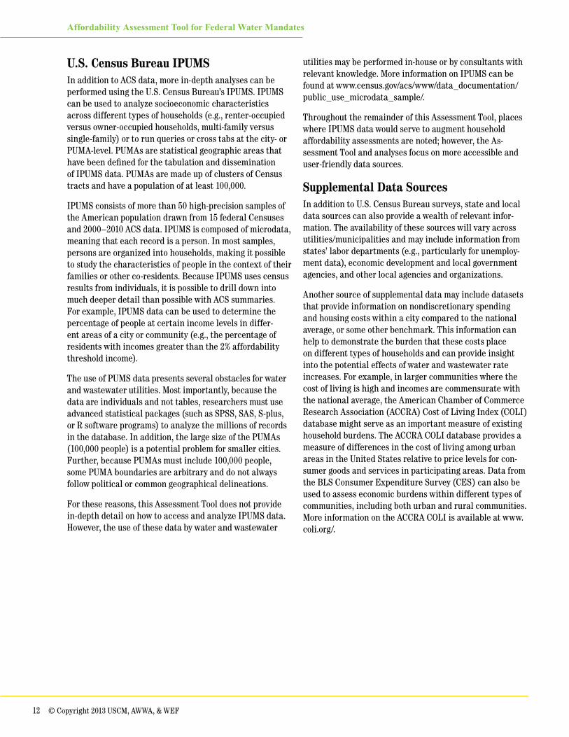
The AFF website provides options for developing maps of income and other socioeconomic data by Census tract. Tract-level data can also be analyzed and mapped using geographic information systems (GIS), depending on the resources and capabilities within your utility. With the use of GIS, utilities have the options for further analyzing the data and conducting more in-depth analyses (e.g., developing maps showing Census tracts where the average household water and wastewater costs exceed specifi c percentages of MHI). Workbook 3, “Socioeconomic Indica-tors” provides specifi c instructions for accessing Census tract-level data and developing the corresponding maps.
Figures 4-1 and 4-2 provide examples of Census tract MHI maps for the City of Philadelphia developed on the AFF website and using GIS, respectively. These maps demon-strate signifi cant variation across census tracts, in terms of MHI. Workbook 2 includes specifi c instructions for down-loading and mapping Census tract level data.
To identify potentially vulnerable populations, income levels should also be analyzed across different types of households. For example, in some communities there may be considerable differences between income levels for renter-occupied and owner-occupied households, as well as between multi-family and single-family households, or between elderly and non-elderly households. Income data for renter and owner-occupied households and for elderly
residents can be downloaded from the 2011 (or relevant year) ACS single-year dataset. However, income data for multi-family and single-family households can only be accessed through IPUMS.
Table 4-1 shows how MHI can vary signifi cantly across different types of households, using Kansas City, Kansas as an example.
In addition, in recent years income levels in many cities have been declining. Where this happens it has important affordability implications because it means that increases in water and wastewater bills will not be offset by similar increases in incomes. Income data can be downloaded from single-year ACS databases from 2005 through the cur-rent year. When comparing MHI across years, it is import-ant to adjust for infl ation (using the CPI) so that all data points are compared using the same year value. For smaller communities, it will be necessary to look at changes in three-year or fi ve-year average ACS estimates.
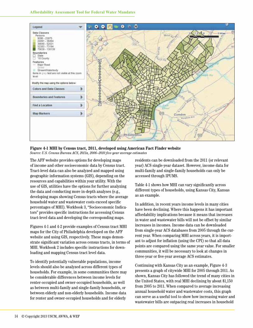
Continuing with Kansas City as an example, Figure 4-3 presents a graph of citywide MHI for 2005 through 2011. As shown, Kansas City has followed the trend of many cities in the United States, with real MHI declining by about $1,150 from 2005 to 2011. When compared to average increasing annual household water and wastewater costs, this graph can serve as a useful tool to show how increasing water and wastewater bills are outpacing real increases in household
Figure 4-1 MHI by Census tract, 2011, developed using American Fact Finder websiteSource: U.S. Census Bureau ACS, 2011a, 2006–2010 fi ve-year average estimates

© Copyright 2013 USCM, AWWA, & WEF 15
Affordability Assessment Tool for Federal Water Mandates
incomes (e.g., annual average household water and waste-water costs can be graphed on the secondary y axis).
Table 4-1 MHI by household type, Kansas City, Kansas
Household type MHI (2011$)
All households 37,036
Elderly households 27,955
Renter-occupied 24,898
Owner-occupied 47,272Source: U.S. Census Bureau ACS, 2012, 2011 single-year estimates
Workbook 3 (an Excel spreadsheet) provides the specifi c ACS data tables you will need to obtain the information presented above for your community. The spreadsheet also provides templates for presenting these indicators as graphs and tables (see spreadsheet tabs MHI, MHI_HHType, and ServiceArea_MHI_2005-2011).
Income DistributionIn many cities, incomes are less centered on the median compared to incomes in the United States as a whole. This has important implications for affordability because
Figure 4-2 MHI by Census tract, 2011, developed using in-house GIS capabilitiesSource: U.S. Census Bureau ACS, 2011a, 2006–2010 fi ve-year average estimates
16 © Copyright 2013 USCM, AWWA, & WEF
Affordability Assessment Tool for Federal Water Mandates
it means that a higher percentage of households within these communities may be adversely impacted by water and wastewater rate increases compared to what might be expected under a more equal distribution of income. Al-though this is the case in many larger urban communities, Rubin (2001b) shows that this is also the case for many rural/nonmetropolitan communities, which tend to have a higher percentage of households in lower-income catego-ries compared to the national average.
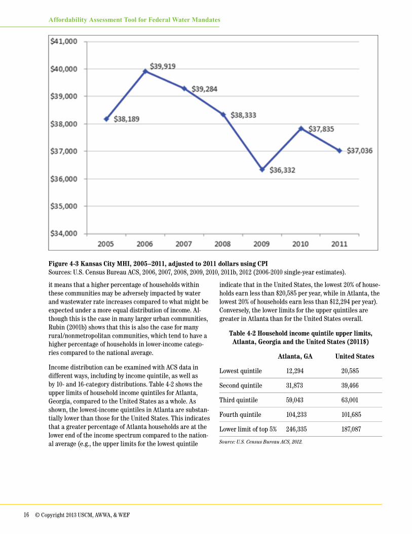
Income distribution can be examined with ACS data in different ways, including by income quintile, as well as by 10- and 16-category distributions. Table 4-2 shows the upper limits of household income quintiles for Atlanta, Georgia, compared to the United States as a whole. As shown, the lowest-income quintiles in Atlanta are substan-tially lower than those for the United States. This indicates that a greater percentage of Atlanta households are at the lower end of the income spectrum compared to the nation-al average (e.g., the upper limits for the lowest quintile
indicate that in the United States, the lowest 20% of house-holds earn less than $20,585 per year, while in Atlanta, the lowest 20% of households earn less than $12,294 per year). Conversely, the lower limits for the upper quintiles are greater in Atlanta than for the United States overall.
Table 4-2 Household income quintile upper limits, Atlanta, Georgia and the United States (2011$)
Atlanta, GA United States
Lowest quintile 12,294 20,585
Second quintile 31,873 39,466
Third quintile 59,043 63,001
Fourth quintile 104,233 101,685
Lower limit of top 5% 246,335 187,087
Source: U.S. Census Bureau ACS, 2012.
Figure 4-3 Kansas City MHI, 2005–2011, adjusted to 2011 dollars using CPISources: U.S. Census Bureau ACS, 2006, 2007, 2008, 2009, 2010, 2011b, 2012 (2006-2010 single-year estimates).

© Copyright 2013 USCM, AWWA, & WEF 17
Affordability Assessment Tool for Federal Water Mandates
Figure 4-4 graphically portrays that the income levels in Atlanta are more concentrated toward the ends of the in-come spectrum compared to the national average. Indeed, the fi gure reveals that the income bracket containing Atlanta’s MHI ($43,903 in 2011) is one of the least-populat-ed income classes in the entire city. Thus, it is evident that in Atlanta (and in many other cities in the United States), citywide MHI does not refl ect a “typical” household. Fur-ther, a much higher percentage of residents would be ad-versely impacted by increased water and wastewater bills compared to communities with a more equal and centrally clustered income distribution.
The evaluation of income distribution across different household types can help to identify vulnerable populations within a community. Continuing with Atlanta, Georgia, as an example, Figure 4-5 shows the income distribution across elderly households (i.e., the head of the household is 65 years or older) compared to the income distribution citywide. As shown, the majority of elderly households
(52%) have a reported income of less than $25,000. This compares to about 33% of households citywide.
As demonstrated in Table 4-1, a second population of potentially vulnerable households includes renter-occu-pied households, which often have lower incomes than owner-occupied households. Figure 4-6 shows the income distribution for renter- and owner-occupied households in Atlanta, Georgia, where 55% of all households are renter occupied. As shown, there is a much higher percentage of renter-occupied households in the lower-income categories, with close to 40% of all renters earning less than $20,000 per year.
Workbook 3 provides the specifi c ACS data tables that you will need to obtain income distribution data for your com-munity. The spreadsheet also provides templates for pre-senting these indicators as graphs and tables (see spread-sheet tabs Inc._quintiles; Inc._dist; Elderly_Inc_dist;, and Renter_Owner_Inc_dist).
Figure 4-4 Income distribution in Atlanta, Georgia and the United StatesSource: U.S. Census Bureau ACS, 2012 (2011 single-year estimates).

18 © Copyright 2013 USCM, AWWA, & WEF
Affordability Assessment Tool for Federal Water Mandates
Figure 4-5 Income distribution in Atlanta, Georgia, elderly households and citywideSource: U.S. Census Bureau ACS, 2012 (2011 single-year estimates)
Figure 4-6 Atlanta, Georgia income distribution, renter- and owner-occupied households Source: U.S. Census Bureau ACS, 2012 (2011 single-year estimates)

© Copyright 2013 USCM, AWWA, & WEF 19
Affordability Assessment Tool for Federal Water Mandates
Poverty RatesIn addition to income levels and income distribution, pover-ty rates serve as an important indicator of economic need. In 2011, 15.9% of people in the United States were living below the federal poverty line. This percentage provides a benchmark for assessing poverty levels within your com-munity, which can be obtained using ACS single-year and three-year average estimates (depending on the size of your service area). Data on the percentage of elderly residents and children living below the federal poverty line are also available through ACS. These data can help to identify vulnerable populations.
Similar to income levels, poverty rates can be examined at the Census tract level using five-year average ACS esti-mates. Once these data are downloaded, they can be used to identify “poverty areas,” where 20% or more of the house-holds in that Census tract have incomes below the federal poverty level. Again, these data can be mapped using AFF or with GIS capabilities at your utility.
In terms of affordability, identifying areas where poverty is more concentrated may have important implications for public health. In essence, the effective reduction in disposable income among low-income households could adversely affect those households’ ability to pay for needed food, heat, and medical care (Crawford-Brown et al., 2009; Raucher et al., 2011). Care should be taken to ensure that public policies (including well-intentioned environmental mandates) do not impose costs that may further exacer-bate the health challenges faced by households in such low-income neighborhoods.
Many have argued that the official (i.e., federal) poverty rate does not provide an accurate measure of the number of households truly living in poverty conditions. Indeed, various studies have emphasized that households with incomes that are significantly higher than the poverty level often experience severe hardships, including hunger, lack of needed heating and cooling, and the inability to afford medical care (Boushey et al., 2001).
To obtain a more accurate measure of households living in poverty conditions, the U.S. Census Bureau developed a Supplemental Poverty Measure (SPM) in 2010. The SPM factors in public assistance and financial support offered to low-income households (e.g., housing subsidies, low-in-come home energy assistance) and also recognizes some nondiscretionary expenses that such households bear (e.g., taxes, out-of-pocket medical expenses, and geographic adjustments for differences in housing costs) (U.S. Census Bureau, 2011a).
At the national level, for a two- adult, two-child household in 2010, the SPM income threshold was set at $24,343. This compares to the official poverty threshold of $22,113. Nationwide, the SPM indicates4 that there are 5.35% more people in poverty than the official poverty threshold would indicate. The SPM also indicates that inside Metropolitan Statistical Areas the difference is 11.2%, and within “prin-cipal cities,” the SPM-implied number of people in poverty is 5.94% higher than the official poverty measure indicates. Although the SPM is not yet available at the city/communi-ty level, these general rules can help to identify additional households that may be adversely impacted by increased water and wastewater rates.
Workbook 3 provides the specific ACS data table that you will need to obtain poverty data for your community. The spreadsheet also provides templates for presenting these indicators as graphs and tables (see spreadsheet tab “Poverty”).
Housing Burdens and Nondiscretionary SpendingAs noted in chapter 1, EPA’s residential indicator does not capture existing household economic burdens beyond those associated with water and wastewater bills. Economic burdens are commonly measured by comparing the cost of particular necessities to the resources (e.g., income) available to a household or community. EPA’s RI is such a measure in that it is used to evaluate the economic burden from wastewater charges by comparing those charges to MHI. However, wastewater service is just one of a set of basic necessities whose costs influence the overall econom-ic burden on a community’s households.
Household economic burdens can be a significant factor for large urban communities where the cost of living is much higher than the national average, as well as in smaller rural communities where MHIs are often lower than the national MHI but nondiscretionary costs are not. Analy-sis of household economic burdens and nondiscretionary spending requirements can provide an indication of how difficult it is for both low- and middle-income households in your community to make ends meet, and how increases in water and wastewater costs will impact different types of households.
Housing burden is the most common measure of household economic burden. Most government agencies consider housing costs of between 30% and 50% of household income to be a moderate burden in terms of affordability; while costs greater than 50% of household income are considered
4 The SPM also adjusts for different housing status (e.g., renters versus owners). Additional details can be found in the U.S. Census Bureau (2011).

20 © Copyright 2013 USCM, AWWA, & WEF
Affordability Assessment Tool for Federal Water Mandates
a severe burden. The ACS provides information on monthly housing costs for both owner-occupied and renter-occupied households, as well as by income level. These data can be divided by the MHI for these different groups to calculate housing burden. Additional analyses can be performed using IPUMS data (e.g., IPUMS can be used to determine the exact number of households with a moderate or severe housing burden, while ACS summary files can only provide average costs as a percentage of MHI for a limited number of household types).
Workbook 3 provides the specific ACS data tables you will need to access to obtain housing burden data for your community. The spreadsheet also provides templates for presenting different housing burden indicators as graphs and tables (see spreadsheet tab “Housing_burden”).
Sources of nondiscretionary spending data can help to pro-vide insight into additional household economic burdens. Key sources for these data include the Bureau of Labor Sta-tistics CES, the ACCRA COLI, and any additional local data sources prepared by government agencies or organizations. The BLS CES contains detailed demographic, income, and monthly expenditure data at the PUMA level. These data can provide insight on relative consumer spending within your community compared to different types of commu-nities (e.g., urban vs. rural). CES data are accessed in the same way that IPUMS data are accessed, and require a thorough knowledge of a statistical software package such as SAS, SPSS, or STATA.
ACCRA COLI data are another source of nondiscretionary spending data. The ACCRA COLI provides a measure of
differences in the cost of living among urban areas in the United States. The ACCRA COLI measures relative price levels for consumer goods and services in participating areas. The average for all participating places, both metro-politan and nonmetropolitan, equals 100 and each partic-ipant’s index is read as a percentage of this average. The ACCRA COLI dataset is updated quarterly for approximate-ly 305 cities within the United States, and includes data for different income quintiles. This data can be useful if your community is one of the participating areas.
Additional Socioeconomic IndicatorsThere are several additional measures of economic need that can help to examine the ability of households to afford water and wastewater rate increases, including:
1. Percentage of residents receiving public assistance income and/or food stamps
2. Average annual unemployment rates
3. Number/percentage of households that are delinquent in paying their water bills
4. Number/percentage of households enrolled in utility low-income assistance programs.
Workbook 2 describes the specific ACS source tables that contain information related to the percentage of residents receiving public assistance income and/or food stamps and average annual unemployment. Information on delinquency rates and low-income assistance programs should be avail-able through your utility.

© Copyright 2013 USCM, AWWA, & WEF 21
Affordability Assessment Tool for Federal Water Mandates
Chapter 5
Guidance for Developing Alternative Measures of Household AffordabilityThis chapter provides additional guidance for assessing water and wastewater affordability at the household level (i.e., going beyond EPA’s RI). This includes the development of utility-specific affordability measures, such as compar-ing current average wastewater bills to household income levels across the income distribution in your service area or community. The following sections provide an overview of recommended approaches for assessing affordability and communicating results, while more detailed instructions and templates for developing these alternative metrics are included in Workbook 4.
Remember that EPA may consider the affordability of water and CSO mandates using your community’s MHI. However, throughout the following sections, water and/or wastewater bills are compared to household income levels, drawing upon data from selected communities throughout the United States. For the purpose of this Assessment Tool, hypothetical average household water and wastewater costs of $300 and $450, respectively, are used for a com-bined average annual bill of $750. It is important to keep in mind that these analyses can be conducted using current water and/or wastewater costs, as well as household water and wastewater costs that take into account planned rate increases. This chapter also provides additional detail on conducting affordability analyses for future years.
Average Water and Wastewater BillsThroughout this chapter, the comparison of average household water and wastewater bills to household income levels are discussed. It is important to note that the use of the term “bill” is intended to reflect the estimated average costs of water and/or wastewater service based on current rates and average household consumption. If data are avail-able, a weighted average can be determined based on the number of single- and multi-family homes in the commu-nity and their respective average household consumption levels.
With this approach, average household water and wastewa-ter costs are based on your utility’s existing rate models, as reflected in the current rates. This provides a more realis-
tic assessment of current household costs and should allow you to easily evaluate household affordability in future years under planned rate increases. This approach should also allow you to examine household affordability under a series of “what if” scenarios (e.g., examining affordability with and without the impact of a potential mandated or nonmandated investment, or under different assumptions regarding interest rates and financing costs).
Water and Wastewater Bills and Household Income ComparisonsAs a first step to developing your affordability indicators, compare average annual water and wastewater bills to household incomes for different types of households and across geographic areas. At the citywide level, this cal-culation essentially represents EPA’s RI (although it can include water costs in addition to wastewater costs). The RI calculation should also be evaluated at the Census tract level (if your community is large enough to include several Census tracts) to identify areas where average household costs may have a “mid-range” to “large” economic impact (e.g., as defined by EPA for wastewater).
Continuing with our analysis of MHI by Census tract for the City of Philadelphia (see chapter 4), Figure 5-1 shows average annual household wastewater costs (using our hypothetical average bill of $450) as a percentage of Census tract MHI. This map demonstrates how an increase in wastewater rates would impact communities within Philadelphia differently.
The Census tracts outlined in black in Figure 5-1 illustrate an important point for analyzing household affordability at the Census tract level. These Census tracts are high-lighted because they have fewer than 750 people in them (the average number of people per Census tract is about 4,000). Thus, although a map may show several Census tracts where the average household water and/or waste-water bill amounts to a relatively high percentage of MHI, it is important to evaluate what this means in terms of the overall population of your service area (in the case of Philadelphia, about 1.5 million people). To account for this,

22 © Copyright 2013 USCM, AWWA, & WEF
Affordability Assessment Tool for Federal Water Mandates
it is important to examine variables that provide context (e.g., population, number of households) when downloading Census tract data for specifi c analyses. These data can be easily downloaded by Census tract via AFF using ACS fi ve-year average estimates.
In many communities, the estimated average household wastewater bill and total combined (water and wastewater) bill may not exceed 2% and 4.5%, respectively, of MHI in most Census tracts; however, a number of households have
incomes well below the MHI for their community. Many of these households may already be paying more than 2% of their income for wastewater services, or more than 4.5% of their income for combined water and wastewater services.
This can be easily examined using income distribution data from the ACS. For example, Figure 5-2 shows the percentage of households within Sacramento, California, at different levels of affordability (i.e., the percentage of households spending certain percentages of their income
Figure 5-1 Hypothetical average annual wastewater bill as a percentage of Census tract MHI, Philadelphia, PennsylvaniaSource: U.S. Census Bureau ACS, 2011a, 2005–2010 fi ve-year average estimates

© Copyright 2013 USCM, AWWA, & WEF 23
Affordability Assessment Tool for Federal Water Mandates
on water and wastewater services). This analysis is based on the percentage of households within each of 16 Cen-sus-defi ned income categories and evaluates the average wastewater and total combined water and wastewater bill as a percentage of the mid-point income within each category. As shown, it appears that with average household costs of $300 and $450 for water and wastewater services, respectively, close to 30% of households in Sacramento, would pay more than 2% of their income for wastewater services, and about 20% pay more than 4.5% of their income for combined water and wastewater services.
IPUMS data can be used to conduct further analysis on the number of households that may be unable to afford signifi cant water and/or wastewater rate increases. For example, based on the estimated average household water and wastewater cost of $750, households earning less than $16,667 would pay more than 4.5% of their income for water and wastewater services. IPUMS can be queried to deter-mine the exact number of households within your com-munity (and within each PUMA in your community), that make less than this amount (and therefore would have paid more than 2% of their income for their estimated average wastewater bill).
Figure 5-2 Hypothetical annual average wastewater and combined water and wastewater bills as a percentage of household income, Sacramento, California
Table 5-1 Hypothetical annual average wastewater bill as percentage of MHI by income category, Butte, Montana
Percentage MHI within Average estimated wastewaterIncome category of households income quintile bill as a percentage of MHILess than $20,000 24% $10,000 7.50%
$20,000 to $39,999 26% $29,999 2.50%
$40,000 to $74,999 30% $57,499 1.30%
$75,000 to $99,999 8% $87,499 0.86%
$100,000 to $199,999 10% $149,999 0.50%
Three-year average ACS estimates were used due to the small size of Butte; one-year estimates are unavailable.

24 © Copyright 2013 USCM, AWWA, & WEF
Affordability Assessment Tool for Federal Water Mandates
Table 5-1 presents another way to evaluate impacts to low-income households within your community. Based on the hypothetical average water and wastewater bill of $750, Table 5-1 shows average annual water and wastewater costs as a percentage of MHI for different income cate-gories, using Butte, Montana, as an example. As shown, average water and wastewater bills already amount to more than 7.5% of MHI for households in the lowest-income category (approximately 24% of the 14,836 households in Butte). This analysis assumes that MHI within each income quintile is the mid-point. However, IPUMS data can be used to determine the true median.
Examining the average wastewater bill as a percentage of poverty level income also provides insight into the number of people facing unaffordable water and wastewater bills. Poverty threshold incomes vary depending on the number of people living in the household. For example, in 2010, the official federal poverty threshold for a household or family of 2 was $15,130; for a family of 4, the poverty threshold was $23,050.
Table 5-2 shows the hypothetical average water and waste-water bill of $750 as a percentage of poverty threshold incomes by household size. To conduct this analysis, the combined water and wastewater bill of $750 were adjusted to account for differences in household size, based on the average U.S. household size of 2.64 in 2011 (i.e., each per-son in the household adds about $284 to the average bill). As shown in Table 5-2, the hypothetical average bill of $750 ranges from 2.5% to 5.8% of poverty threshold incomes.
Finally, as discussed in chapter 4, in many communities, incomes vary considerably between renter-occupied and owner-occupied households, as well as for elderly house-holds. Drawing upon our analysis of MHI for different types of households in Kansas City, Kansas (see chapter 4), Table 5-3 shows an average total water and wastewater bill of $750 as a percentage of MHI across these different household types. As shown, in Kansas City renter-occupied households have much lower incomes than all other house-hold types. On average, these households would pay 3.01% of their income for water and wastewater services with an average annual bill of $750.
Table 5-2 Hypothetical annual average wastewater bill as a percentage of federal poverty threshold incomes
Household or Average water and Estimated average household family size Poverty threshold wastewater bill (example) bill as a percentage of ($) poverty level income (%)
1 $11,170 284 2.54%
2 $15,130 568 3.76%
3 $19,090 852 4.46%
4 $23,050 1,136 4.93%
5 $27,010 1,420 5.26%
6 $30,970 1,705 5.50%
7 $34,930 1,989 5.69%
8 $38,890 2,273 5.84%

© Copyright 2013 USCM, AWWA, & WEF 25
Affordability Assessment Tool for Federal Water Mandates
Table 5-3 Hypothetical annual average total household water and wastewater bill as a percentage of MHI by household type, Kansas City, Kansas
Household MHI Average household type (2011$) water and wastewater cost as a percentage of MHI
All households 37,036 2.03%
Elderly households 27,955 2.68%
Renter-occupied 24,898 3.01%
Owner-occupied 47,272 1.59%
Source: U.S. Census Bureau ACS, 2012 (2011 single-year estimates).
IPUMS data can also be used to estimate average house-hold water and wastewater costs as a percentage of MHI for multi-family and single-family homes. For this analysis, the average estimated water and wastewater bill can be based on actual average consumption for these different types of households.
Workbook 4 provides specific instructions and templates for developing the affordability metrics (including graphs and tables) presented in this section. The “Overview” tab is this spreadsheet contains a table of contents that links spread-sheets in the Excel worksheet to specific figures and tables in this section.
Income Distribution: Implications for Wastewater Affordability
As noted throughout this report, EPA’s 1997 Guidance suggests that wastewater bills equal to 2% of MHI are considered affordable for a community. In 1997 (when the Guidance was developed), the most recent income and poverty data available would have been from 1996. In 1996, the national MHI was $35,492 (U.S. Census Bureau, 1997). Thus, an average annual wastewater bill equal to 2% of na-tional MHI would have equated to $710. Based on national income distribution data, in 1996 the lowest quintile (20th percentile) of household income was 42% of the median income, or approximately $14,900 (U.S. Census Bureau, 1997). That is, the lowest 20% of households in the United States made $14,900 or less. At that income level, a bill of $710 would have equated to 4.75% of household income. In other words, the MHI threshold of 2% would be equivalent to having 20% of households in a community pay 4.75% (or more) of their income for wastewater service.
Using the national income distribution data for 2012, a bill equal to 2% of national MHI would be $1,010 per year. That bill would represent 4.9% (or more) of income for the lowest 20% of U.S. households, which is relatively similar to the 1996 level. In many communities, however, a wastewater bill of 2% of MHI would have a much more severe impact on low-income households. For example, in New York City, 2% of the city’s MHI of $49,461 would be $989 per year. This would represent 5.9% at the upper limit of the city’s lowest income quintile ($16,824), meaning that at least one-fifth of the city’s households would be paying 5.9% of their income (or more) for wastewater services—a burden that is 20% greater than would be expected from the national income distribution.
In this example for New York City, in order to keep the impact on low-income households consistent with that expected from national income distributions—that is, to ensure that no more than 20% of households face sewer bills of 4.8% (or more) of income—then wastewater bills would need to be no more than $807 per year, or 4.8% of the upper limit for the lowest income quintile. This amounts to 1.63% of the city’s MHI. This reveals the extent to which the 2% of MHI metric does not reflect burdens on the poorest 20% of households in the community, and that an MHI-based metric of affordability for New York City of about 1.6 would be more equivalent to 1996 measures for reflecting impacts on the lowest-income quintile.
This analysis can be easily applied to your community in the context of water and/or wastewater services using ACS data related to income quintiles and MHI.
Assessment of Affordability in Future YearsFinally, in addition to analyzing affordability impacts associated with current water and wastewater rates, it is also important to examine how affordability will change over time. Many utilities have the capability to estimate rate increases for future years, based on estimated costs associated with planned projects and programs. Using these data, it is relatively straightforward to calculate the estimated average household water and wastewater bill for future years. However, this calculation will need to take into account any assumed changes in household water consumption over time, such as whether your utility expects average household use to decline. You may also want to conduct sensitivity analyses to examine the effect of your assumptions (e.g., regarding O&M costs for planned projects or project financing costs and interest rates).

26 © Copyright 2013 USCM, AWWA, & WEF
Affordability Assessment Tool for Federal Water Mandates
In order to compare average water and wastewater bills to household income levels, it will also be necessary to make some assumptions about how income levels will change over time. In the past, we would have recommended that you simply assume incomes will increase at the same rate as the CPI. However, as demonstrated in chapter 6, in recent years income levels have not kept pace with the CPI, and have even declined in many communities. This can make it difficult to project MHI for your community going forward.
One approach for projecting future income levels is to examine how income levels have changed in recent years in comparison to the CPI. For example, over the past five years national income levels have increased at a rate of approximately 60% of the increase in CPI. Given the recent economic crisis and recovery process, it seems reasonable to assume that this trend will likely continue, at least for the near future. Thus, to project MHI over the next several years, you may wish to assume that incomes will increase by about 60% (or rate at which your community’s MHI has increased relative to CPI) of the forecasted change in CPI (as developed by the Congressional Budget Office). Beyond
the next several years, it may be reasonable to assume that incomes will again begin to increase at the same rate as the CPI. Although this analysis is not exact, it does provide a general idea of how income levels may change.
Communicating the Results
Given the wealth of information and analyses described in chapters 4 and 5 of this Assessment Tool, it can be difficult to imagine how to best synthesize and communicate the results of your affordability assessment. As noted in chap-ter 4, we do not propose any specific thresholds that would indicate that a community is at risk of being unable to afford significant increases in water and wastewater costs. The analyses conducted here are intended to go beyond EPA’s RI to provide a more comprehensive assessment of household affordability.
Depending on your community, you may want to focus on specific aspects of the Assessment Tool suggested (e.g., EJ concerns, elderly households, impacts to low-income house-holds). The graphs and tables portrayed in this Assessment Tool are also provided as templates in the guidance docu-ments and can be used to analyze and present results.
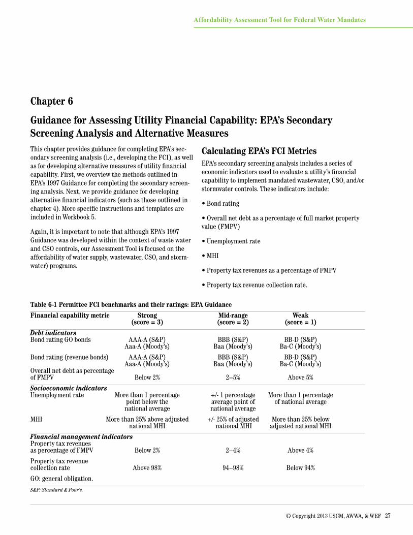
© Copyright 2013 USCM, AWWA, & WEF 27
Affordability Assessment Tool for Federal Water Mandates
Chapter 6
Guidance for Assessing Utility Financial Capability: EPA’s Secondary Screening Analysis and Alternative MeasuresThis chapter provides guidance for completing EPA’s sec-ondary screening analysis (i.e., developing the FCI), as well as for developing alternative measures of utility financial capability. First, we overview the methods outlined in EPA’s 1997 Guidance for completing the secondary screen-ing analysis. Next, we provide guidance for developing alternative financial indicators (such as those outlined in chapter 4). More specific instructions and templates are included in Workbook 5.
Again, it is important to note that although EPA’s 1997 Guidance was developed within the context of waste water and CSO controls, our Assessment Tool is focused on the affordability of water supply, wastewater, CSO, and storm-water) programs.
Calculating EPA’s FCI MetricsEPA’s secondary screening analysis includes a series of economic indicators used to evaluate a utility’s financial capability to implement mandated wastewater, CSO, and/or stormwater controls. These indicators include:
• Bond rating
• Overall net debt as a percentage of full market property value (FMPV)
• Unemployment rate
• MHI
• Property tax revenues as a percentage of FMPV
• Property tax revenue collection rate.
Table 6-1 Permittee FCI benchmarks and their ratings: EPA Guidance
Financial capability metric Strong Mid-range Weak (score = 3) (score = 2) (score = 1)
Debt indicators Bond rating GO bonds AAA-A (S&P) BBB (S&P) BB-D (S&P) Aaa-A (Moody’s) Baa (Moody’s) Ba-C (Moody’s)
Bond rating (revenue bonds) AAA-A (S&P) BBB (S&P) BB-D (S&P) Aaa-A (Moody’s) Baa (Moody’s) Ba-C (Moody’s) Overall net debt as percentage of FMPV Below 2% 2–5% Above 5%
Socioeconomic indicators Unemployment rate More than 1 percentage +/- 1 percentage More than 1 percentage point below the average point of of national average national average national average
MHI More than 25% above adjusted +/- 25% of adjusted More than 25% below national MHI national MHI adjusted national MHI
Financial management indicators Property tax revenues as percentage of FMPV Below 2% 2–4% Above 4%
Property tax revenue collection rate Above 98% 94–98% Below 94%
GO: general obligation.
S&P: Standard & Poor’s.

28 © Copyright 2013 USCM, AWWA, & WEF
Affordability Assessment Tool for Federal Water Mandates
As part of the screening analysis, each indicator is “scored” on a scale of 1 (weak) to 3 (strong). The average of these scores represents the overall FCI. The following sections describe the methods and data sources used to determine each indicator. Table 6-1 shows the ratings and scores for each indicator, as outlined in EPA’s guidance documents.
Bond rating The first financial benchmark included in EPA’s secondary screening analysis is a municipality’s bond rating for both GO and revenue bonds. GO bonds are bonds issued by a local government and repaid with taxes (usually property taxes). GO bond ratings reflect financial and socioeconom-ic conditions experienced by the community as a whole. Revenue bond ratings, by comparison, reflect the financial conditions and management capability of a water/wastewa-ter utility. They are repaid with revenues generated from user fees.
There are currently three major rating agencies for mu-nicipal bonds: Moody’s Investors Services, S&P, and Fitch Ratings. Of the three rating agencies, Moody’s and S&P’s rate over 80% of all municipal and corporate bonds (these are also the only two rating agencies included in EPA’s 1997 Guidance). Municipal bond reports from these agencies can be accessed at:
• Moody’s Investors rating service: www.moodys.com
• S&P rating service: www.standardandpoors.com
Table 6-1 shows how ratings from these agencies translate into “strong,” “mid-range,” and “weak” scores in terms of the FCI.
In its 1997 Guidance, EPA notes that there are many small- and medium-sized communities that have not used debt fi-nancing and therefore have no bond rating. EPA states that when a bond rating is unavailable, this indicator can be excluded from the secondary screening analysis. However, this will effectively place a greater reliance on scores for the socioeconomic and financial management indicators.
Net debt as a percentage of Fair Market Property Value (FMPV)The second financial benchmark measures a municipal-ity’s outstanding GO debt as a percentage of FMPV. This indicator is intended to provide a measure of debt burden on residents within your service area/community, as well as a measure of the ability of your local government to issue additional debt.
To calculate net debt as a percentage of FMPV, it is first necessary to identify the direct net debt of your communi-ty, as well as your community’s share of debt from overlap-ping entities. EPA defines overall net debt as debt repaid by property taxes within a utility/municipality’s service area. It excludes debt that is repaid by special user fees (e.g., revenue bonds). The percentage of your community’s share of debt from overlapping entities is the amount charged to persons or property with your service area (based on the estimated FMPV of real property of each overlapping jurisdictions).
Debt information is typically available from your commu-nity’s annual financial statements. FMPV data should be available through your community or State assessor’s office (EPA’s 1997 Guidance states that as long as your service area boundaries generally conform to one or more commu-nity boundaries, it is not necessary to prorate the FMPV).
In some communities, the tax assessed property value will not reflect FMPV. This occurs when the tax assessment ra-tio is less than one. In such cases, FMPV can be computed by dividing the total tax assessment value by the assess-ment ratio (i.e., the percentage of the FMPV that is taxed at the established tax rate).
If the net debt for your community is greater than 5% of the FMPV, you would receive a “weak” rating for this indicator, based on EPA’s scoring methodology. A net debt of 2% to 5% of FMPV is considered “mid-range,” while below 2% is considered “strong.”
Unemployment rateThe unemployment rate is defined as the percentage of the total labor force that is unemployed but actively seeking employment and willing to work. Monthly and annual average unemployment rates are available through the BLS Local Area Unemployment Statistics (LAUS) program. LAUS is a federal-state cooperative effort that maintains employment statistics for Census regions and divisions (e.g., counties and metropolitan statistical areas), cities of 25,000 population or more, and other areas. EPA Guidance does not specify whether monthly or annual data should be used, however, we recommend using the annual average unemployment rate. For more information and to access LAUS data, visit www.bls.gov/lau/data.htm.
For the purposes of calculating the overall FCI, local unemployment rates are compared to the national average as a benchmark (also available through BLS). Areas with an unemployment rate of more than 1% above the national average are rated as “weak” in this area. Areas with unem-

© Copyright 2013 USCM, AWWA, & WEF 29
Affordability Assessment Tool for Federal Water Mandates
ployment rates within 1% of the national average is consid-ered “mid-range” and those with unemployment rates more than one percentage point below the national average are considered “strong.”
MHIThe MHI benchmark compares your community’s MHI to the national MHI. As detailed in previous chapters, this information can be easily accessed from the U.S. Census Bureau ACS via AFF. Depending on the size of your commu-nity, you will need to use single-year, three-year average, or five-year average ACS estimates. These estimates are adjusted for inflation by the ACS.
In terms of the overall FCI, a community is considered weak for this indicator if MHI is more than 25% below the national MHI, mid-range if MHI is within 25% of the national MHI, and strong if MHI is more than 25% above the national MHI.
Tax revenues as a percentage of FMPVThis indicator, which EPA also refers to as the “property tax burden,” is intended to measure the funding capac-ity available to support debt based on the wealth of the community, as well as the effectiveness of management in providing community services (1997 Guidance).
FMPV data should be readily available through the commu-nity or state’s assessor office, while property tax revenues are typically available in a community’s annual financial statements. If a community’s property tax revenues are greater than 4% of FMPV, a “weak” rating is assigned for this indicator; between 2% and 4% is considered mid-range; and below 2% is considered strong.
Property tax collection rateThe property tax collection rate is intended to measure of the efficiency of the tax collection system and the accept-ability of tax levels to residents. To determine the collec-tion rate, you will need to divide property tax revenues by the property taxes levied. However, be aware that this metric may understate the effort your community is mak-ing if it relies less than the typical community on property taxes and more on, say, sales taxes, user fees, special fees, and assessments. See the following section for more on this issue.
To calculate property taxes levied, multiply the assessed value of real property within your community/service area by the property tax rate. This information should
be available through your community or state assessor’s office. Property tax revenues are typically available in your community’s annual financial statements.
For this indicator, if the property tax collection rate in your community is below 94%, you will receive a “weak” rating; between 94% and 98% is considered mid-range; and above 98% is considered “strong.”
Alternative Measures of Utility Financial CapabilityChapter 1 of this Assessment Tool provides several sugges-tions for supplemental measures that would help to provide a better assessment of utility financial capability. The following sections provide instructions for developing and analyzing these measures.
It is important to note that the measures suggested below may not necessarily apply to your community, and that there may be additional financial indicators not reflected here that may be particularly relevant for your communi-ty. In developing evidence to support a determination on whether your utility has the financial capability to imple-ment regulatory mandates, it is important to investigate relevant measures and metrics specific to your community.
Local tax revenues as a percent of gross taxable resourcesAs discussed previously, EPA uses property tax revenues as a percentage of FMPV as its sole measure of local tax burden. However, in cities that rely on multiple forms of taxation, focusing solely on property taxes inevitably un-derstates a city’s current tax effort. To account for multiple forms of taxation, total local tax revenues as a percentage of gross taxable resources should be included as a supple-mental measure in EPA’s FCI (in addition to real property taxes as a percentage of FMPV). This would provide a better measure of the extent to which a municipality is already using the full range of its taxable resources.
Gross taxable resources are the combined dollar amount of resident household incomes and business surpluses (income less employee compensation) within a community (NYC Independent Budget Office, 2007). Tax effort is the ratio of direct and overlapping government tax collections to taxable resources. In 2007, the NYC Independent Budget Office developed a report comparing state and local taxes in large U.S. cities (NYC Independent Budget Office, 2007). This report provides a methodology for determining a city/municipality’s total taxable resources and is available at

30 © Copyright 2013 USCM, AWWA, & WEF
Affordability Assessment Tool for Federal Water Mandates
www.ibo.nyc.ny.us/iboreports/CSALTFINAL.pdf. Total tax revenues should be available within your community’s annual financial reports.
Measuring the severity of unemploymentChapter 1 of this Assessment Tool discusses the limitations associated with the application of current annual average unemployment as a key indicator of utility financial capa-bility. To provide a more accurate measure of whether local economic problems are severe enough to warrant relief from EPA mandates, the following measures are suggested:
• The current and long-term average unemployment rate in your community compared to the long-term national average. Between 1991 and 2011, the national unemploy-ment rate averaged 5.8%. Use of the long-term average level of unemployment as a benchmark anchors the national unemployment rate as a comparison measure. For example, in 2010 a community with an unemployment rate of 10.1% would be classified as having only a mid-range unem-ployment problem simply because it was within 1% of the national average of 9.1% in that year.
• Long-term unemployment compared to national long-term unemployment. The annual average unemployment rate does not reflect trends in long-term unemployment (defined as the share of the labor force continuously un-employed for one half year or more). Use of the long-term unemployment rate provides an additional measure of economic distress within a community.
In addition to broadening the range of labor market indicators, other measures of local economic distress, such as foreclosure rates and annual migration/population data, can provide insight into the financial capability of a
community or utility to fund mandated programs. In many communities, high foreclosure rates have had a significant impact on the financial condition of local governments, and their ability to finance capital improvements. In addition, chronic joblessness leads working-age residents to migrate to areas where they have a better chance of finding a job. This kind of migration does not show up in unemployment rates, but it can permanently affect a community’s ability to support investments in water and wastewater systems.
The deterioration of local government financial capabilities To take into account the erosion of local government finances, a measure of local government revenue growth or decline can be included in EPA’s FCI matrix, with an absolute decline in real revenues over some period taken as a sign of weakened financial capacity. Revenue growth or decline should be measured over a long enough period of time to ascertain a trend (e.g., the last 3 to 5 years). This information should be available from your local govern-ment’s annual financial reports.
Ignoring other long-term liabilitiesEPA’s methodology for assessing municipalities’ financ-ing capacity takes into account their formal debt burden (measured by the ratio of net debt to underlying property values). But it does not consider a burden that for a growing number of municipalities is greater than the burden of for-mal debt—unfunded pension liabilities and other commit-ments to retirees, as well as other long-term contractual commitments. The value of unfunded long-term liabilities over time should be included as a supplemental measure of utility financial capability (e.g., in comparison to available resources for meeting these commitments).

© Copyright 2013 USCM, AWWA, & WEF 31
Affordability Assessment Tool for Federal Water Mandates
BibliographyBoushey, H., C. Brocht, B. Gundersen, and J. Bernstein. 2001. Hardships in America: The Real Story of Working Families. Economic Policy Institute, Washington, DC.
CRA Infrastructure & Engineering. 2011. Financial Capa-bility Assessment for the Draft Long Term Control Plan. Prepared for Buffalo Sewer Authority, Buffalo, New York by CRA Infrastructure & Engineering, Inc.
Crawford-Brown, D., R. Raucher, S. Rubin, and M. Lawson. 2009. Risk Trade-offs in Public Health when Water Prices Rise: The Implications for Small Community Supplies. White Paper for National Rural Water Association. Avail-able at www.nrwa.org/whitepapers/afford/RiskTrade-offs_inPublicHealthWhenWaterPricesRise.doc
NDWAC. 2003. Recommendations of the National Drinking Water Advisory Council to U.S. EPA on Its National Small Systems Affordability Criteria. US EPA National Drinking Water Advisory Council.
NYC Independent Budget Office. 2007. Comparing State and Local Tax Burdens in Large U.S. Cities. New York City Independent Budget Office. February.
Raucher, R.S., S.J. Rubin, D. Crawford-Brown, and M.M. Lawson. 2011. Benefit-Cost Analysis for Drinking Water Standards: Efficiency, Equity, and Affordability Consid-erations in Small Communities, Journal of Benefit-Cost Analysis 2(1):Article 4. Available at www.bepress.com/jbca/vol2/iss1/4. Accessed 6/15/2011.
Rubin, S.J. 2001a. Affordability of Water Service. Issue Brief, National Rural Water Association.
Rubin, S.J. 2001b. Economic Characteristics of Small Sys-tems. Issue Brief, National Rural Water Association.
Rubin, S.J. 2003. Update of Affordability Database, Issue Brief, National Rural Water Association.
Stavins, R., G. Long, and J. Jaffe. 2004. Assessment of the Economic Impact of Additional Combined Sewer Overflow Controls in the Massachusetts Water Resources Authority Service Area.
U.S. Census Bureau. 1997. Current Population Reports, P60-197, Money Income in the United States: 1996 (With Separate Data on Valuation of Noncash Benefits), U.S. Government Printing Office, Washington, DC.
U.S. Census Bureau ACS. 2006. 2005 Single-year Estimates. U.S. Census Bureau American Community Survey.
U.S. Census Bureau ACS. 2007. 2006 Single-year Estimates. U.S. Census Bureau American Community Survey.
U.S. Census Bureau ACS. 2008. 2007 Single-year Estimates. U.S. Census Bureau American Community Survey.
U.S. Census Bureau ACS. 2009. 2008 Single-year Estimates. U.S. Census Bureau American Community Survey.
U.S. Census Bureau ACS. 2010. 2009 Single-year Estimates. U.S. Census Bureau American Community Survey.
U.S. Census Bureau. 2011a. The Research Supplemental Poverty Measure: 2010. U.S. Department of Commerce, Economics and Statistics Administration. November.
U.S. Census Bureau ACS. 2011b. 2005–2010 Five-year Aver-ages. U.S. Census Bureau American Community Survey.
U.S. Census Bureau ACS. 2011c. 2010 Single-year Estimates. U.S. Census Bureau American Community Survey.
U.S. Census Bureau ACS. 2012. 2011 Single-year Estimates. U.S. Census Bureau American Community Survey.
USDOL BLS. 2012. Consumer Price Index. Available at www.bls.gov/cpi
U.S. EPA. 1997. Combined Sewer Overflows – Guidance for Financial Capability Assessment and Schedule Develop-ment. EPA 832-8-97-004. U.S. Environmental Protection Agency, Office of Water, Office of Wastewater Management. Available at www.epa.gov/npdes/pubs/csofc.pdf.
USEPA, 1995, Interim Economic Guidance for Water Quality Standards Workbook.
U.S. EPA. 2002. Affordability Criteria for Small Drinking Water Systems: An EPA Science Advisory Board Report. EPA-SAB-EEAC-03-004. U.S. Environmental Protection Agency, Washington, DC.
U.S. EPA. 2006. Small Drinking Water Systems Varianc-es – Revision of Existing National-Level Affordability Methodology and Methodology to Identify Variance Tech-nologies that are Protective of Public Health. EPA-HQ-OW-2005-0005; FRL-8035-7. Federal Register 71(41). March 2. Washington, DC.


