... • .. Axial Behavior of Damaged Tubular Columns by Joseph A. Padula Alexis Ostapenko Sponsored by Minerals Management Service of the U.S. Department of the Interior (Contract No. 14-12-0001-30288) and American Iron and Steel Institute (Project No. 338) DOIIAISI COOPERATIVE RESEARCH PROGRAM Fritz Engineering Laboratory Report No. 508.11 Lehigh University September 1989
Transcript
...
•
..
Axial Behavior of Damaged Tubular Columns
by
Joseph A. Padula
Alexis Ostapenko
Sponsored by
Minerals Management Service
of the U.S. Department of the Interior
(Contract No. 14-12-0001-30288)
and
American Iron and Steel Institute
(Project No. 338)
DOIIAISI COOPERATIVE RESEARCH PROGRAM
Fritz Engineering Laboratory Report No. 508.11
Lehigh University
September 1989
LEGAL NOTICE
This report was prepared as an account of government-sponsored work. Neither the United States, nor the Minerals Management Service of the Department of the Interior, nor any person acting on behalf of the Minerals Management Service of the Department of the Interior
(A) Makes any warranty or representation, expressed or implied, with respect to the accuracy, completeness or usefulness of the information contained in this report, or that the use of any information, apparatus, method, or process disclosed in this report may not infringe privately owned rights; or
(B) Assumes any liabilities with respect to the use of or for damage resulting from the use of any information, apparatus, method, or process disclosed in this report.
As used in the above, "persons acting on behalf of the Minerals Management Service of the Department of the Interior" includes any employee or contractor of the Minerals Management Service of the Department of the Interior to the extent that such employee or contractor of the Minerals Management Service of the Department of the Interior prepares, handles, or distributes, or provides access to any information pursuant to his employment or contract with the Minerals Management Service of the Department of the Interior.
•
..
Table of Contents Abstract 1. Introduction
1.1 Problem Definition 1.2 Previous Research 1.3 Need for Research 1.4 Work Performed
2. Development of the Database 2.1 Database Management 2.2 Included Data
3. Generation of Analytical Data 3.1 Idealized Geometry of a Damaged Column 3.2 Basic Concepts of the Finite Element Model 3.3 Finite Element Discretization 3.4 Verification of Calculated Response
4. Approximation of Load-Shortening Behavior 4.1 Regression Analysis 4.2 Parametric Study
4.2.1 Selection of Coordinate Functions 4.2.1.1 Coordinate Function for A. 4.2.1.2 Coordinate Function for D/t 4.2.1.3 Coordinate Function for d/D 4.2.1.4 Coordinate Function for o/L 4.2.1.5 Coordinate Function for S
4.2.2 Formulation of the Regression Model 4.3 Fit to Existing Data 4.4 Example Calculation 4.5 Range of Applicability
5. Summary, Conclusions and Recommendations 5.1 Summary and Conclusions
5.1.1 Finite Element Computer Analysis 5.1.2 Database for Axial Behavior of Damaged Compression Members
5.2 Selection of Parameters 5.2.1 Selection of Coordinate Functions 5.2.2 Development of Approximate Engineering Method 5.2.3 Limitations of the Method
5.3 Recommendations for Future Work 5.3.1 Extension of Current Work 5.3.2 Further Research on Damaged Tubular Members
5.3.2.1 Dented and Crooked Members 5.3.2.2 Corroded Members 5.3.2.3 Members with Fatigue Cracks
List of Figures Figure 1: Basic Concept of Finite Element Model 34 Figure 2: Damaged Column Geometry 35 Figure 3: Dent Geometry 35 Figure 4: Shell Element Discretization of Modell 36 Figure 5: Shell Element Discretization of Model 2 37 Figure 6: Shell Element Discretization of Model 3 38 Figure 7: Comparison of Experimental Results with Models 1, 2 and 3 39 Figure 8: Boundary Conditions and Constraints 40 Figure 9: Domain Defining Smooth Load-Shortening Response 41 Figure 10: Finite Element Model 3 and Experimental Load- 42
Shortening for Specimen men (Ref. [12]) Figure 11: Finite Element Model 3 and Experimental Load- 43
Shortening for Specimen A4 (Ref. [8]) Figure 12: Finite Element Model 3 and Experimental Load- 44
Shortening for Specimen B3 (Ref. [8]) Figure 13: Finite Element Model 3 and Experimental Load- 45
Shortening for Specimen RIA (Ref. [10]) Figure 14: Sample Data for Selection of Coordinate Function for/.., 46 Figure 15: Sample Data for Selection of Coordinate Function for /.., 47 Figure 16: Sample Data for Selection of Coordinate Function for D/t 48 Figure 17: Sample Data for Selection of Coordinate Function for D/t 49 Figure 18: Sample Data for Selection of Coordinate Function for diD 50 Figure 19: Sample Data for Selection of Coordinate Function for diD 51 Figure 20: Sample Data for Selection of Coordinate Function for o/L 52 Figure 21: Sample Data for Selection of Coordinate Function for o/L 53 Figure 22: Typical Inverse Load-Shortening Relationship 54 Figure 23: Coordinate Function for S 55 Figure 24: Approximation of Load-Shortening for Specimen A3 (Ref 56
[8]) Figure 25: Approximation of Load-Shortening for Specimen B3 (Ref 57
[8]) Figure 26: Approximation of Load-Shortening for Specimen RIA 58
(Ref [10]) Figure 27: Approximation of Load-Shortening for Specimen men 59
(Ref [12]) Figure 28: Approximation of Load-Shortening for Analysis ST A3 _17 60
(ADINA) Figure 29: Approximation of Load-Shortening for Analysis STA3_56 61
(ADINA)
..
iii
List of Tables Table 1: Data Included in Database Table 2: Data Included in Regression Analysis
31 32
1
Axial Behavior of Damaged Tubular Columns
by Joseph A. Padula and Alexis Ostapenko
Fritz Engineering Laboratory Report No. 508.11
September 1989
Abstract
A simple "engineering" method was formulated for computing the axial load vs. axial shortening relationship of pin-ended tubular members damaged by a dent and/or out-ofstraightness. The method predicts the pre- and post-ultimate load-shortening response, and can be used in analyzing the strength and behavior of offshore platform frames containing such damaged members. The method was developed from a parametric study and regression analysis of a database containing load-shortening data from published tests results on small-scale damaged specimens (31 load-deformation curves) and data generated from a finite element analysis (56 load-deformation curves).
The effects of geometric nonlinearity and elasto-plastic material property were included in the finite element analysis of the pre- and post-ultimate response of damaged tubular columns. Prior to generating data for the parametric ·study and -regression analysis, the finite element model was verified by comparing calculated (finite element) loadshortening responses with small-scale test data.
In order to develop a regression model to be used as a basis for the simplified engineering method, a parametric study was conducted to determine the influence of each independent variable on the axial behavior of damaged members. The object of the study was to select the shortest suitable approximating (coordinate) function for each independent variable. The variables considered were: column slenderness, D/t ratio, dentdepth to diameter ratio, out-of-straightness, yield stress, and axial shortening. The regression analysis of the load-shortening relationships in the database resulted in a set of 96 constants which is reduced to a four-term approximating function for the load-shortening response, once specific values are given for the member geometry, material and damage. The procedure is illustrated with some examples and a comparison with test results.
The method is valid for member geometries and material properties typically found in fixed offshore platforms with the limitation that relatively thick-walled members should have sustained significant damage. This limitation is based on the exclusion of members which exhibit a sharply peaked load-deformation relationship. ·
2
1. Introduction
The design of offshore structures must include considerations of strength, stability, and
serviceability while providing for safe and reliable resistance to applied loads over the life of
the structure. From monitoring and inspection of in-service platforms, it has become in
creasingly apparent that these basic requirements must be met for the structure in a
deteriorated condition, i.e., the structure must be designed with some degree of damage
tolerance. "Damage-tolerance may especially be crucial for deep-water fixed platforms,
where inspection and maintenance of the deeply submerged parts of the structure may be
difficult, if not impossible." [2] Minimum requirements are derived from consideration of
the consequences of structural failure: loss of human life, of the structure, and/or environ
mental pollution. These dictate that. operational and environmental loads must not result in
collapse or progressive failure of the structure, particularly as a result of slight or undetected
damage. Furthermore, the economy of operation/maintenance of a platform requires that a
structure should have the capacity to withstand some minimal damage without the need for
costly repairs.
Although some degree of damage tolerance is implicit in any redundant structure,
quantification of the residual strength of a damaged member(s) and of the whole structure is
needed for a rational approach to efficient, cost-effective design and maintenance. Con
sequently, the research described in this report was directed at the assessment of the effect of
accidental damage on member behavior, whether anticipated as in the design process or real
as a result of accidental overload on an in-service platform.
1.1 Problem Definition Typically the effect of dents and/or out-of-straighmess of a tubular. member results in a
reduction of the stiffness and/or capacity of the member and this may significantly affect the
strength and/or serviceability of the structure. The remaining residual strength of the struc
ture is dependent on the pre- and post-ultimate behavior of the damaged member since it is
likely that service loads will lead to non-linear response of the damaged member resulting in
a redistribution of forces in the structure. Therefore, the response of the damaged member
must be known or estimated in order to assess the effect of damage on the structure.
3
In general, prediction of the pre- and post-ultimate load-shortening response of
damaged tubular columns requires a shell analysis of the member including the effects of
large deformations and material nonlinearity. However, analysis of this type is impractical
even if possible with state-of-the-an finite element programs. Consequently, there is a need
for a simplified yet reasonably accurate "engineering method" for predicting the behavior of
damaged members.
1.2 Previous Research In one of the first reported efforts to quantify the effects of damage in tubular members,
a parametric study was made using finite element analysis of initially crooked tubular
columns and experiments on small-scale specimens. [8] However, this was a beam-column
analysis in which distortion of the cross section was not considered. In a later attempt to
include the effect of dent damage, it was suggested that the effect of dents may be included
in the analysis, not by modeling the geometry of the dent, but by retaining the circular cross
section of the member and modifying the stress-strain relationship for fibers in the dent af
fected area. [10] A reduction or "knock-down" factor applied to .the modulus of elasticity
and yield stress was suggested based on empirical data from small-scale tests.
In a series of papers, Taby presented an analytical method which estimates the load
deformation response of dented and/or initially crooked, simply supported
columns. [11, 12, 14, 15] This approach is based on a simplified physical model for which
the governing relations have been fit to empirical data from 109 small-scale tests. The com
puter program DENT A is based on this method. [16]
Ellinas quantified the effect of dent-damage with a lower bound prediction of the ul
timate strength based on first yielding of a simplified physical model similar to Taby's. [1]
In their experimental work Taby and Smith carried out a number of tests on damaged
(dented and crooked) small-scale specimens made from drawn tubing or cold-rolled
plate. [8, 10, 11, 14, 15] From the tests of two large-scale members removed from an off
shore platform retired from service and of two comparable small-scale specimens, Smith
concluded that small-scale tests were adequate to predict the behavior of full-size damaged
members. [9] However, the results of these tests showed that the small-scale specimens un-
4
derestimated the ultimate strength by as much as 15% and the post-ultimate strength by as
much as 30%. Smith attributed the discrepancy in the post-ultimate range to the effect of
different load vs. displacement control in the tests for the large- and small-scale specimens.
1.3 Need for Research While it is possible to predict, with reasonable accuracy, the response of a damaged
member by a finite element analysis using shell elements and including material non
linearity and large deformations, such an analysis is impractical in terms of cost, computer
resources needed, and the time required to formulate a reliable model. Futhermore, analysis
of an entire platform or even a sub-frame containing a damaged member with such a model r
would be even more impractical. Even if a non-linear finite element analysis could be per-
formed efficiently, the results must be independently verified.
Of the approaches discussed above, only Taby's method (DENT A) includes the effect
of cross-sectional distortion and estimates the load-shortening response in the pre- and post
ultimate ranges. However, DENTA is based on a simplified beam-column model that was
"tuned" to experimental results from small-scale tests. The .application of Smith's method
may be limited to members with relatively low D/t ratios since it has been reported that the
effect of cross-sectional deformation (amplification of dent-depth) is significant for D/t
ratios as low as 40. [15] The research reported here represents a phenomenological approach
based on experimental data and analytical data from a general shell finite element analysis.
1.4 Work Performed The objective of this research was to produce a relatively simple yet reasonably ac
curate engineering method for predicting axial load as a function of axial shortening of
damaged, pin-ended, tubular steel columns. The basic approach to the problem centers on
the collection of experimental and generation of analytical column load-shortening
responses followed by a parametric study and a regression analysis of the data, and formula
tion of a simplified method of analysis. This approach has been used successfully in the
past to predict the pre- and post-ultimate response to in-plane loading of plates and stiffened
plates and th~ load-indentation response of circular tubes. [3, 4, 5, 6]
The resulting simplified approximation of load-shortening behavior is a matrix of 96
5
coefficients which, for a given column with known geometry, damage and material, are
reduced to a 4-term function for approximating the load-shortening behavior. The method
can readily be implemented as a subroutine or a stand-alone program.
The work reported here includes the development of a database, the development of an
analytical (fmite element) model for generating additional load-shortening data, and the
development of a regression model. Application of the resulting engineering method is also
demonstrated.
The basic approach to the problem consisted of the following steps: 1. Collection and generation of experimental and analytical data on the load
shortening behavior of damaged columns. a. Literature search for published experimental data.
b. Finite element analysis to generate additional data. i. Development of a model and verification with experimental
results.
ii. Generation of analytical data.
2. Approximation of load-shortening response. a. Parametric study of the data and selection of suitable approximation
functions for the regression model.
b. Regression analysis and improvement of the model (an iterative procedure).
Details of these tasks are described in the following chapters.
6
2. Development of the Database
The development of an approximate method for predicting the load-shortening
response of damaged tubular columns was based on a parametric study and a regression
analysis of analytical and experimental load-shortening relationships contained in a
database. Experimental data was collected from available literature, and analytical data was
generated by a finite element analysis (See Chap. 3).
2.1 Database Management A relational database was needed for managing the database in order to avoid storing
all related data (geometry and material properties of the column) for each point of every
load-shortening curve. An efficient system for storing relatively large amounts of data and
the ability to program custom tailored manipulations of the stored data was also needed.
The capability to produce graphical displays of data was desired to aid in the parametric
study. After reviewing several mainframe and personal computer software packages, the
SAS* software system was selected because of it capabilities to perform all these tasks. The
SAS software was available on a Digital.Equipment Corporation VAX 8530.
2.2 Included Data For each case, the database included the basic data on column geometry (diameter,
thickness, length, dent-depth, initial out-of-straightness), material yield strength, and pairs of
load-shortening coordinates. At least ten points were included for each column, typically
thirteen to eighteen depending on the length of the post-ultimate load-shortening curve. Re
lated parameters (D/t, 8/L, A., etc.) were readily calculated from the raw data for the
parametric study and regression analysis through custom written SAS programs.
Published experimental load-shortening relationships were available from the empirical
work done in this area by other researchers. Principally, published data was taken from
Smith [8, 9, 10] and Taby [12, 13, 14, 15]. Although, in Taby's research, over 100 tubes
*SAS Institute, Cary, N.C.
7
had been tested with a variety of end conditions, only a representative sampling of load
shortening curves were published, all of which (pin-ended tests) were included in the
database.
Analytical data generated by finite element .analysis (See Chap. 3) were .also incor
porated into the database to expand it over a broader range of column geometry and damage.
The number of load-shortening curves included in the database from each source and the
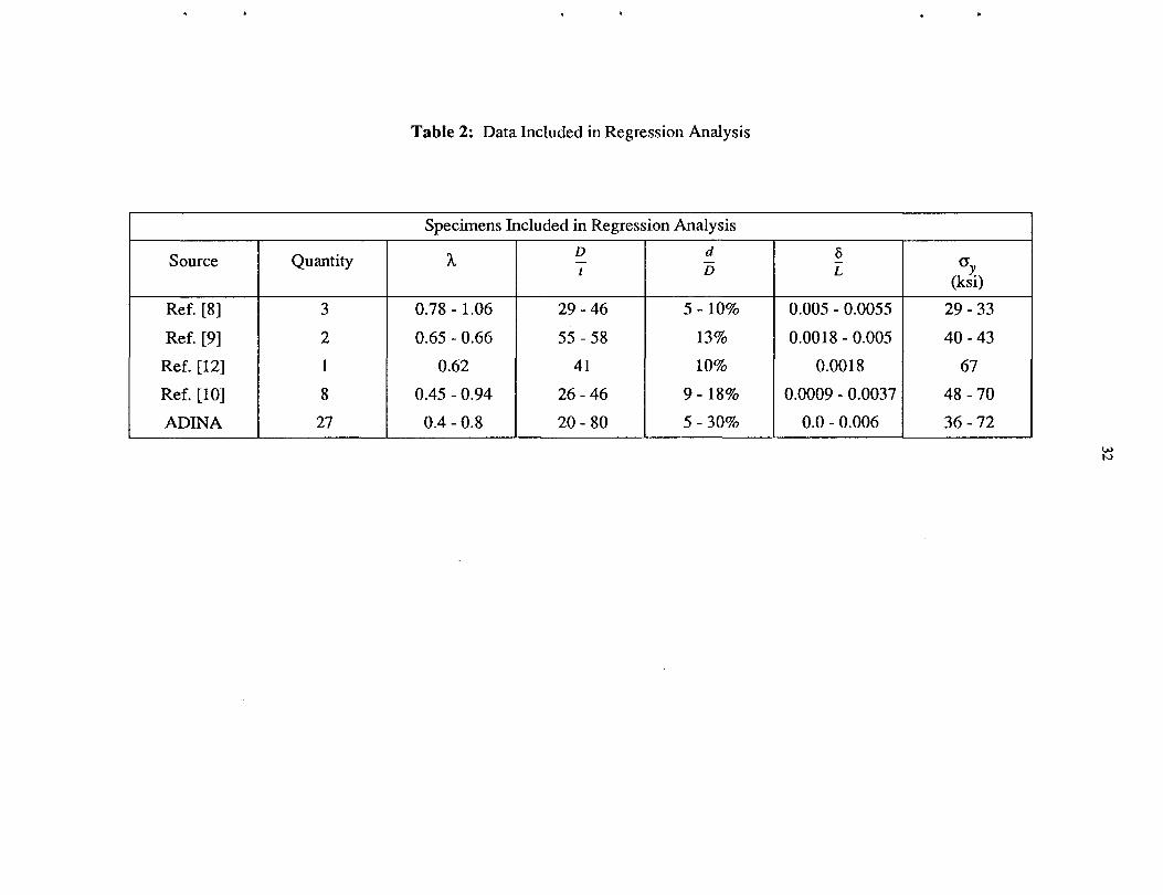
range of geometrical parameters, yield strength and damage are shown in Table 1.
Load-shortening relationships for columns with relatively minor damage and high D/t
ratios presented some difficulty in the simulation process and, at present, were excluded
from the regression analysis. The curves included and their source are listed in Table 2.
8
3. Generation of Analytical Data
In order to effectively study the behavior of damaged tubular columns, additional data
were needed to supplement the limited number of published experimental load-shortening
curves. Due to the complexity of the behavior of a damaged tubular member and the need to
generate data on the pre- and post-ultimate response including large deformations and
material nonlinearity, a finite element analysis was used. The 1984 version of the finite
element software ADINA** (ADINA 84) was selected because of its capabilities for non
linear analysis and automatic load incrementation. The analysis was performed on a Control
Data Corporation Cyber 850 Model180 running the NOSNE operating system.
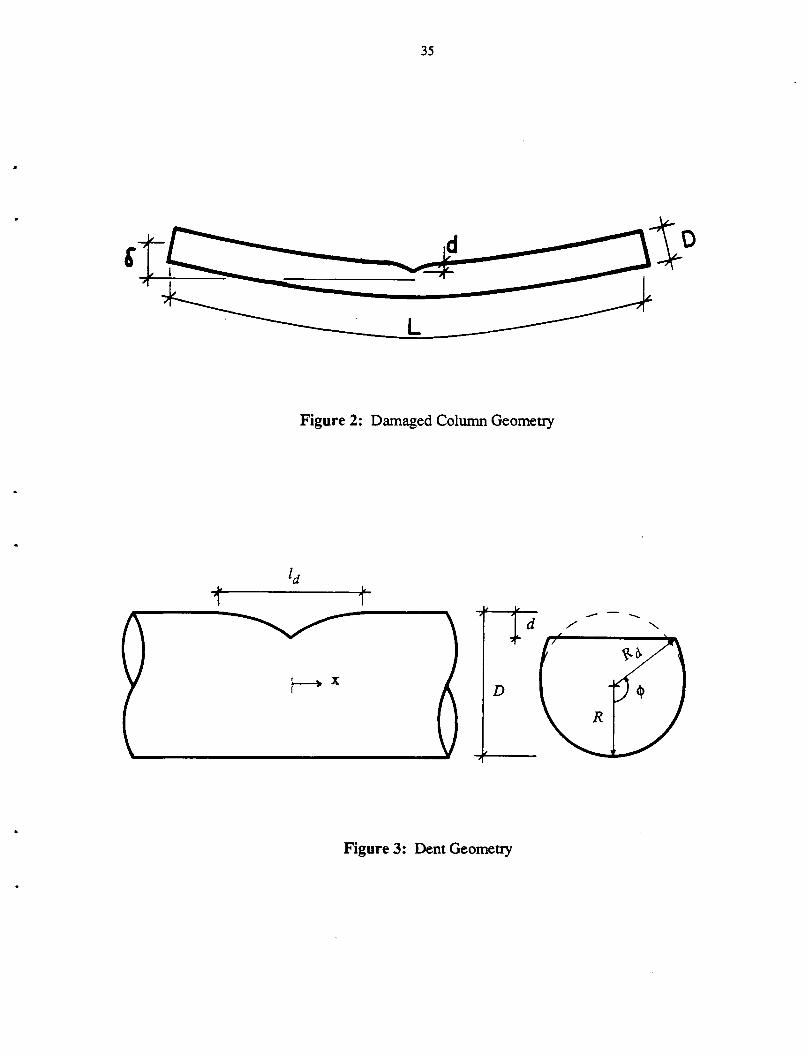
3.1 Idealized Geometry of a Damaged Column In the development of the finite element model for generating data on .. the load
shortening response, certain assumptions were made about the location-and geometry of the
dent damage and the initial out-of-straightness. The idealized geometry permitted descrip
tion of the damage in terms of only two parameters: dent depth d, and-the magnitude of the
initial crookedness (out-of-straightness) 0.
A damaged tubular member with initial crookedness and a dent at mid-length has two
planes of symmetry, one longitudinal and one at the dent perpendicular to the longitudinal
axis, assuming that the dented cross section is symmetrical about the longitudinal plane of
symmetry. (This is a reasonable assumption if the dent and out-of-straightness are caused
by the same accident.) Although dent damage and initial crookedness may have much more
general forms, the longitudinal location of the dent and variations in the shape of the dent
and crookedness have been found by other researchers to have little effect on the behavior.
For example, Smith concluded that "Comparison of test results ... indicates radical variations
in the position of a dent and associated bending damage do not substantially. change the
damage effect" [10], and "Test results also support previous theoretical fmdings that loss of
strength is insensitive to the shape and location of dents and to the shape of bending
**ADINA R & D Inc., Watertown, MA
9
deformation". [1 0] Funher verification comes from Taby, who concluded "The sensitivity
to dent shape and location is, however, insignificant ... ". [13] Consequently, a single
damage model (assumed dent geometry, location and shape of initial crookedness) was used
in the analysis.
The longitudinal axis defining the initial crookedness of the damaged member was as
sumed to be of sinusoidal shape. Thus, for the origin at midlength, it is given by
z=ocos~x L
(1)
where x is the longitudinal distance from mid-length of the column, o is the magnitude of
maximum initial lateral deflection, and z is the lateral deflection of the longitudinal axis of
the tube as shown in Fig. 2. Thus, the initial crookedness is defined by a single parameter,
0.
The dent was assumed to be a sharp "vee" as if produced by a "knife-edge" loading
perpendicular to the longitudinal axis. The geometry of the dent was defmed in terms of the
dent depth, d, as shown in Fig. 3. The longitudinal profile of the dent, ~.and the length of
the dent, ld, were taken from an analytically derived relationship for a tube supported along
its length with no end restraint and subjected to a "knife-edge" lateral loading. [17] The
dent depth as a function of distance from its center at mid-length of the column ( ~ = ~ (x) )
is given by
~=d( 1- ~: / (2)
where
(3)
with D =mean (mid-thickness) diameter of the tube. The expression for ld (Eq. 3) is in
good agreement with dent profiles published by Smith. [10]
The cross-sectional geometry of the dent is based on empirical observations and is
composed of a flattened and a curved segment. The curved segment is defined by the radius
which varies linearly as a function of the angle cp as shown in Fig. 3. The radius increases
from R (the radius of the undamaged tube) to Rd at the intersection of the curved and flat
tened segments. Rd is determined from the requirement that the circumferential length of
the dented and circular cross sections must be equal.
10
(4)
This equation is readily transformed into
R+Rd d-R nR = -- cos-1 (-) + ..JRi-(R-d)2 (5)
2 Rd
which gives Rd, although not explicitly, in terms of Rand d. The discontinuous slope at the
intersection of the flattened and curved segments, as shown in Fig. 3, corresponds to the
plastic hinge formed during indentation.
3.2 Basic Concepts of the Finite Element Model The basic concepts employed in the finite element modeling of the damaged column
are illustrated in Fig. 1. Because of double symmetry of the problem (one longitudinal plane
of symmetry and one plane of symmetry at mid-length), it was only necessary to model
one-quarter of the tube. In addition to the symmetry of the problem, the model reflects the
behavior of the column. For pin-ended boundary conditions, a portion of the column some
distance away from the dent behaves as an elastic beam-column with no distortion of the
cross section. The region near the dent is subjected to bending of the tube wall leading to
distortion of the cross section and plastic deformations. These considerations are reflected
in the model (See Fig. 1) where the region near and including the dent is modeled with shell
elements while the remainder of the column with beam-column (line) elements.
The length of the portion of the column modeled with shell elements was taken to be
one-half the length of the dent, ld, as determined from Eq. 3 plus twice the diameter. An
elastic-plastic material model was used for the shell elements. The remainder of the column
was modeled with beam (beam-column) elements with large displacement formulation and
linearly elastic material. A rectangular cross section was used for the beam elements with
the area and moment of inertia equal to those of the undamaged (circular) cross section.
3.3 Finite Element Discretization The finite element model used to generate load-shortening data was one of three
models developed. The validity of each model was assessed by analyzing test specimens for
which published experimental data were available and comparing the calculated and empiri-
11
cal responses. The models differed primarily in the pattern of discretization and the type
and number of shell elements used in modeling the portion of the column near the dent.
The first model, Model 1, was found to be inadequate for predicting the response of
columns with D/t ratios greater than 60. Model 2 (the second in the series) was much more
accurate but was extremely costly in terms of CPU time. Model 3 exhibited good correla
tion with experimental data and was much more economical than Model 2 and therefore was
selected for generating data included in the database.
The discretization of the portion of the tube modeled with shell elements for Model 1 is
shown in Fig. 4. Eighteen 16-node "quadrilateral" and four 9-node "triangular"
isoparametric elements were used. Reasonable results were obtained with this model when
compared to experimental data for tubes with a D/t ratio less than 60. For D/t greater than
60, the model significantly overestimated the strength with the error increasing ap
proximately linearly with the D/t ratio. This was due to the inability -of the model to simu
late the amplification of the dent that coincides with attainment of the ultimate load for tubes
with relatively large D/t.
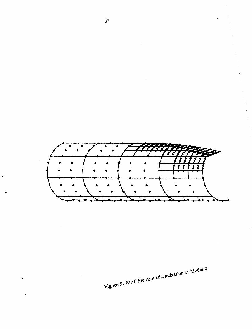
In order to improve the predictions of Model 1, a fmer discretization of the dented area
was used for Model2, and 16-node elements were incorporated as shown in Fig. 5. Model2
resulted in much improved correlation with experimental data for tubes with larger D/t.
However, the model was extremely expensive to use in terms of CPU time. This led to the
development of Model 3.
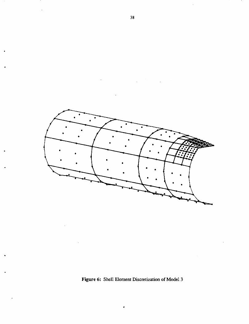
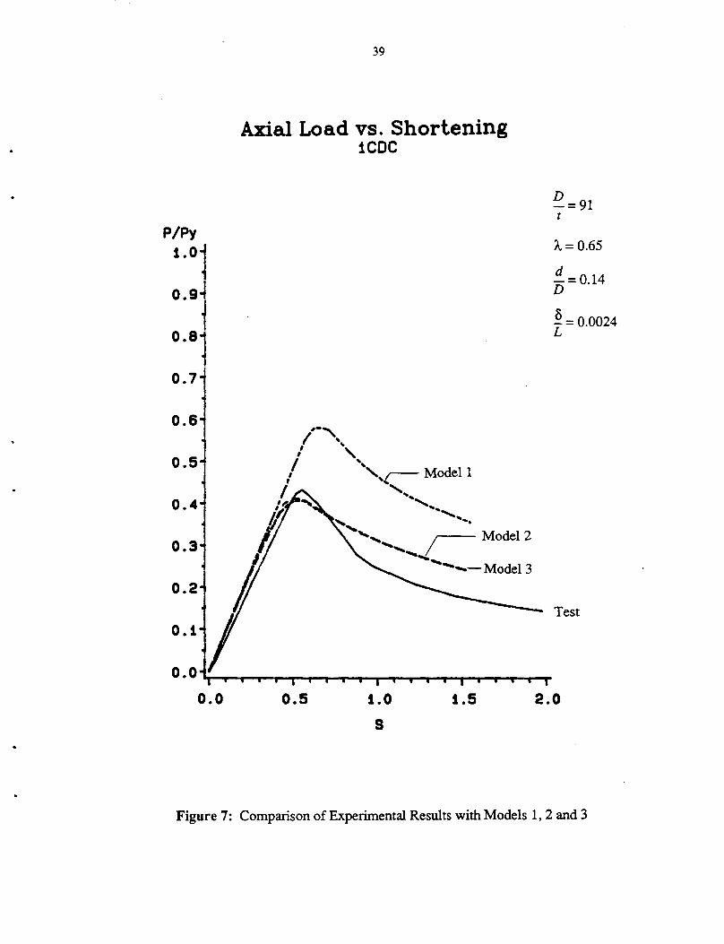
The discretization of Model 3 is shown in Fig. 6 and it resulted in a much more
economical computer usage than Model 2 while producing reasonable agreement with ex
perimental data. Consequently, Model 3 was selected for generating data for the database.
A comparison of the predicted responses from the three models, compared to experimental
data, is shown in Fig. 7. The experimental data is from test specimen 1 CDC with D/t=91,
A=0.65 d/0=0.141% and O/L=0.0024.(Ref. [14])
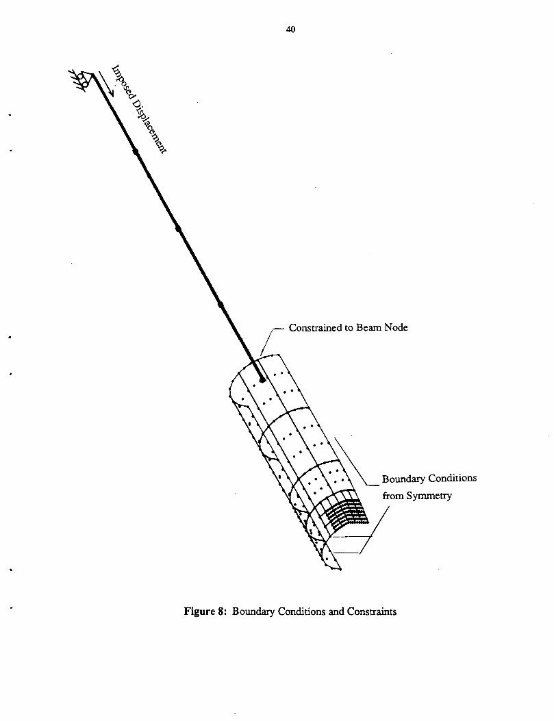
Model 3 had 32 shell elements, 4 beam elements, 268 nodes, and 1162 degrees of
freedom. The shell elements were either 16-node elements or a variation of these needed for
transition from the fmer mesh at the dent to a coarser mesh outside the dent. Boundary
12
conditions were imposed on the nodes at the edges of the shell elements to reflect the sym
metry of the model as indicated in Fig. 8. Nodes lying in a plane of symmetry are allowed
to displace only within and have vectorial rotation perpendicular to the plane of symmetry.
At the junction of the beam and shell elements, the displacements of the shell element nodes
were constrained to the beam element node so that a section through the model remained
plane (See Fig. 8). Lateral displacements of the shell element nodes and of the end node of
the beam element at the juncture were constrained to be equal. Thus, due to symmetry, the
beam elements were planar and had only lateral displacement and bending rotation.
The loading was applied to the model by imposing a displacement in the longitudinal
direction to the end node of the beam element as shown in Fig. 8.
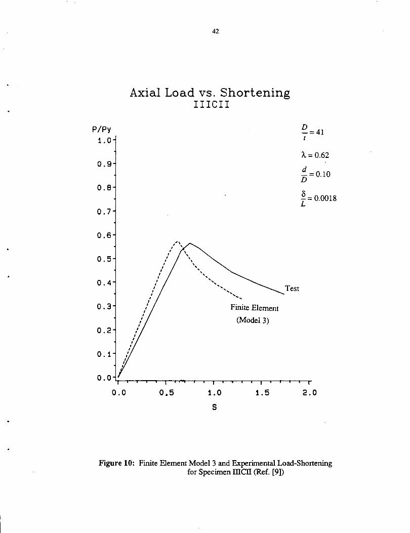
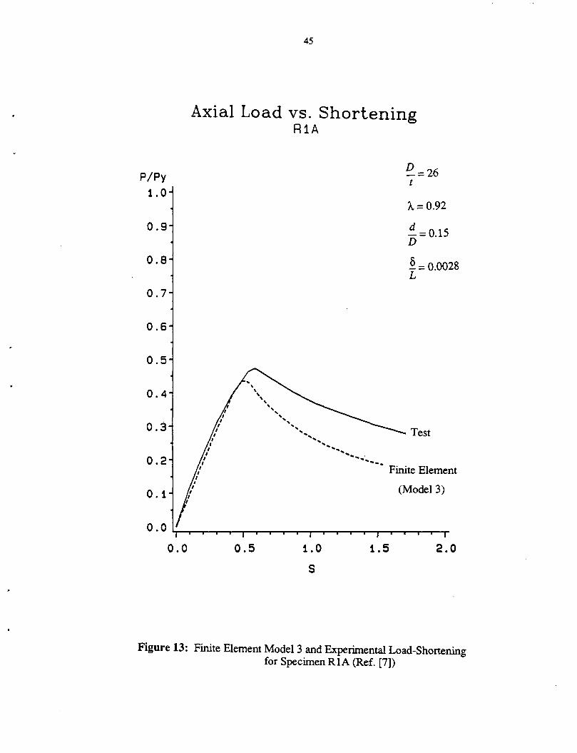
3.4 Verification of Calculated Response The load-shortening curves calculated with Model 3 are shown compared to ex
perimental data in Figs. 10 through 13 as well as in Fig. 7 which shows the calculated results
from Models 1, 2 and 3 for Specimen 1CDC from Ref. [14]. The correlation with ex
perimental data shown in the figures is representative for all others. "In general, the finite
element analysis (Model 3) accurately. predicted the ultimate load of the test specimen. The
calculated responses in the post-ultimate range generally underestimated the load compared
to the experimental data with a few exceptions (See Fig. 7).
13
4. Approximation of Load-Shortening Behavior
A regression analysis was performed on the database to develop a simplified method
for predicting the load-shortening behavior of damaged tubular columns. A brief overview
of the regression method used and specifics with respect to the analysis of the load
shortening behavior are given in the following sections.
4.1 Regression Analysis A multiple linear regression analysis was used to approximate the discrete data in the
database. The known values of the dependent variable (for l data points) are arranged in a
column matrix, F.
(6)
F = , h
For each value, ft, of the dependent variable there is a set, ( x 1i, x2 i, ... , xk i, ... , x n i ), of
corresponding values for n independent variables. The approximation, f , to the data, F, is
taken to be in the form of a linear series.
(7)
where aj are the regression coefficients and qj are the regressors. Each regressor qj is a
function of the independent variable(s). In matrix notation, Eq. 7 can also be expressed by
the product
f = QA (8)
where Q is a 1 x m row matrix of regressors qj and A is a m x 1 column matrix of the coef
ficients, at Coefficients A are determined by solving the following set of linear equations
which are derived from a least squares regression.
BTB A = BTF (9)
Each ith row of matrix B is the row matrix Q evaluated for a set of values of the independent
14
variables corresponding to the itb element of F. Thus, B is a l x m matrix and the product
BTB is am x m matrix.
In multiple regression analysis it is convenient to study separately the effect of each
independent variable on the dependent variable and select a suitable approximating (coor
dinate) function for it. The relationship between the dependent variable and an independent
variable is observed while all other independent variables are kept constant, and an ap
propriate coordinate function is selected to approximate the relationship. In effect, the ele
ments of the coordinate function are regressors for the particular variable and, analogously
to Eq. 8, the approximation, f, can be expressed in terms of a set of coefficients and func
tions of a single independent variable while all other independent variables are set to have
constant values. Thus,
(10)
where Hk is the coordinate function (a row matrix) and Ak is .the column of :coefficients for
the Jctb independent variable. After coordinate functions are selected for each independent
variable, it is assumed that regressors qj which define the approximation f as a function of
all the independent variables in Eq. 7. are formed as a product of the coordinate functions for
the individual independent variables. In this study, the convention of a direct product was
used to establish the regression model from the selected coordinate functions. For example,
for a relationship with n independent variables, the coordinate functions would be desig
nated by the following row matrices:
Hl = [hu h12 hlmll (11)
H2=[h21 h22 ~m] 2
Regressors are then determined by the direct product defined as a prescribed sequence of
multiplications of the elements of the n coordinate functions Hk as indicated below in the
row matrix ofEq. 12.
15
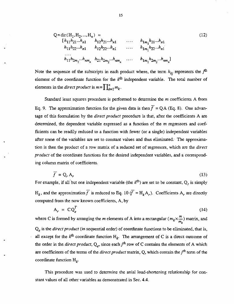
Q=dir(H1,H2, ... ,Hn) = (12)
[ h11 h21···hnl h12h21···hnl
hu~2···hnl h12h22···hnl
hlm h2m ... hnm ] I 2 n
Note the sequence of the subscripts in each product where, the term hkj represents the ;1h
element of the coordinate function for the fCh independent variable. The total number of
elements in the direct product is m = rr~l mk.
Standard least squares procedure is performed to determine the m coefficients A from
Eq. 9. The approximation function for the given data is then/ = QA (Eq. 8). One advan
tage of this formulation by the direct product procedure is that, after the coefficients A are
determined, the dependent variable expressed as a function of the m regressors and coef
ficients can be readily reduced to a function with fewer (or a single) :independent variables
after some of the variables are set to· constant values and thus eliminated: The approxima
tion is then the product of a row matrix of ·a reduced set of regressors, which are the direct
product of the coordinate functions for the desired independent variables, and a correspond
ing column matrix of coefficients.
(13)
For example, if alf but one independent variable (the A;th) are .set to be constant, Qr is simply
Hk, and the approximation/ is reduced to Eq. 10 (j = HkAr). Coefficients Ar are directly
computed from the now known coefficients, A, by
T Ar = CQe (14)
where Cis formed by arranging them elements of A into a rectangular (mkx!!!_) matrix, and mk
Qe is the direct product (in sequential order) of coordinate functions to be eliminated, that is,
all except for the A;th coordinate function Hk" The arrangement of C is a direct outcome of
the order in the direct product, Qe, since each fh row of C contains the elements of A which
are coefficients of the terms of the direct product matrix, Q, which contain the fh term of the
coordinate function Hk"
This procedure was used to determine the axial load-shortening relationship for con
stant values of all other variables as demonstrated in Sec. 4.4.
16
4.2 Parametric Study The database of experimental and analytical load-shortening relationships was used to
establish a set of variables which could defme the behavior of damaged columns. The effect
of each variable was then studied so that suitable coordinate functions could be selected. It
was desirable to select a set of independent variables which result in a minimal scatter of the
data and thus produce a better "fit". In this study, the non-dimensionalized parameters, D/t,
L/r, d/D, o/L and ML were studied with respect to PIP y· Note that for reasons discussed in
Sec. 3.1, the dent shape and location were not included as variables in the study. It was
found that the non-dimensionalized axial load (P/P y) could be represented as a function of
the following parameters: L_t-
1. A=- "\'Ey 1tr
2. D/t
3. d/D
4. o/L ~ 5. S=-
Le.Y
(15)
With these parameters, there was little scatter in the data for wide variations in the absolute
size of the columns and yield stress of the material, and they were used as the independent
variables in the regression analysis. In the notation used in Sec. 4.1 with respect to the order
in the direct product, H1 is the coordinate function for the variable A, H2 is the coordinate
function for D/t, etc., as numbered above in Eq. 15.
In studying the load-shortening response, it was observed that for columns with a rela
tively small amount of damage (dent damage and initial crookedness) and large D/t ratios,
the behavior was characterized by an essentially linear response up to the ultimate load fol
lowed by very rapid decrease in load ("peaked" response). This peaked response was also
observed to be a function of the slenderness (A) of the column. For columns with greater
damage, the load-shortening response was smoother, with a gradual approach to the ultimate
load and a gradual reduction in load in the post-ultimate range.
Due to the difficulty in selecting coordinate functions to depict both types of behavior,
the current study was limited to columns with a relatively smooth load-shortening response.
For this purpose, it was convenient to combine both dent damage and initial out-of
straightness into one "damage factor" u.
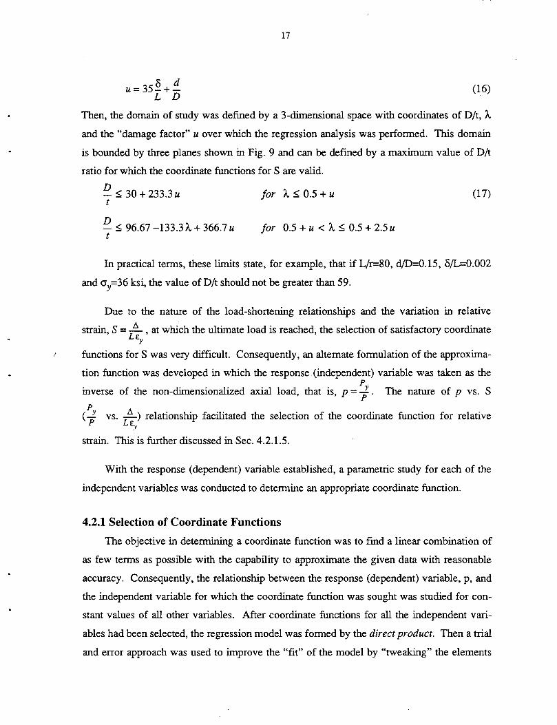
8 d u=35-+L D
17
(16)
Then, the domain of study was defined by a 3-d.imensional space with coordinates of D/t, A
and the "damage factor" u over which the regression analysis was performed. This domain
is bounded by three planes shown in Fig. 9 and can be defmed by a maximum value of D/t
ratio for which the coordinate functions for S are valid.
D - ~ 30 + 233.3u t
D - ~ 96.67 -133.3A + 366.7 u t
for A~ 0.5 + u (17)
for 0.5 + u < A ~ 0.5 + 2.5 u
In practical terms, these limits state, for example, that if L/r=80, d/0=0.15, 8/L=0.002
and cry=36 ksi, the value of D/t should not be greater than 59.
Due to the nature of the load-shortening relationships and the variation in relative
strain, S = ~ , at which the ultimate load is reached, the selection of satisfactory coordinate LEY
functions for S was very difficult. Consequently, an alternate formulation of the approxima
tion function was developed in which the response (independent) variable was taken as the p
inverse of the non-dimensionalized axial load, that is, p = ; . The nature of p vs. S p
( 2 vs. ~) relationship facilitated the selection of the coordinate function for relative P LEY
strain. This is further discussed in Sec. 4.2.1.5.
With the response (dependent) variable established, a parametric study for each of the
independent variables was conducted to determine an appropriate coordinate function.
4.2.1 Selection of Coordinate Functions
The objective in determining a coordinate function was to fmd a linear combination of
as few terms as possible with the capability to approximate the given data with reasonable
accuracy. Consequently, the relationship between the response (dependent) variable, p, and
the independent variable for which the coordinate function was sought was studied for con
stant values of all other variables. After coordinate functions for all the independent vari
ables had been selected, the regression model was formed by the direct product. Then a trial
and error approach was used to improve the "fit" of the model by "tweaking" the elements
18
of the coordinate functions. illustrative examples of the basis for the selection of the coor
dinate functions for each variable are given in the following sections. Note that some terms
of the coordinate functions were multiplied by a factor of a power of ten so that the in
dividual terms would all have approximately the same order of magnitude. This was done to
preclude any numerical difficulties in the solution of Eq. 9 associated with a badly scaled
solution vector A (large variation in the orders of magnitude).
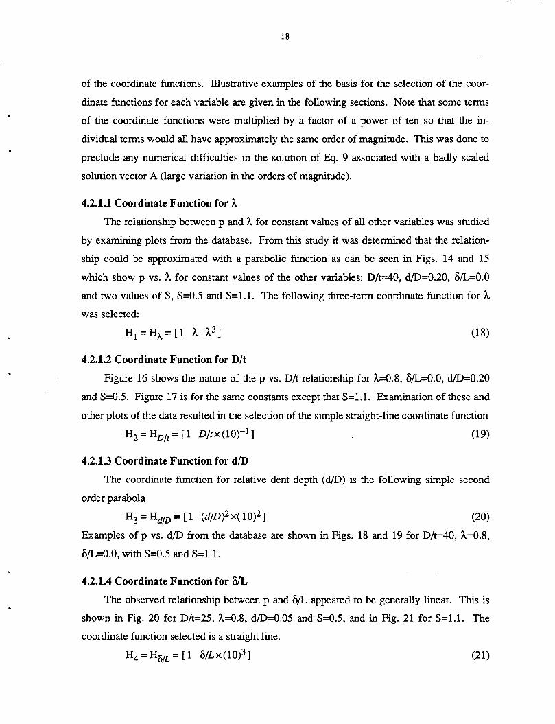
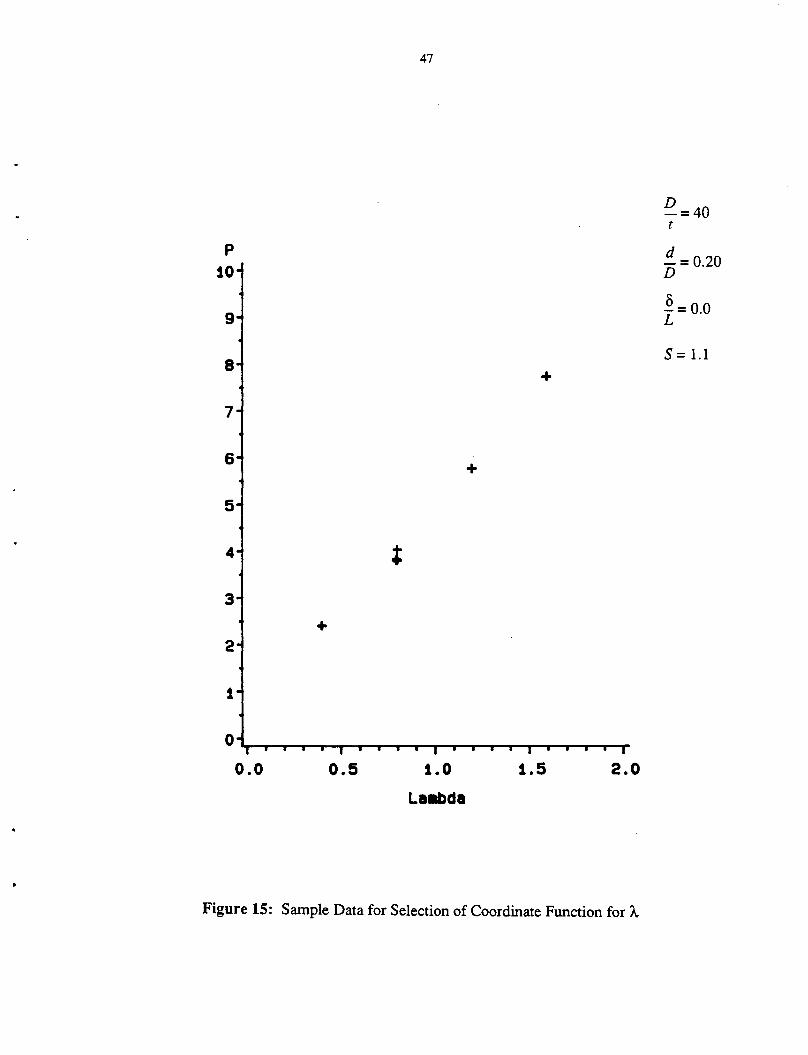
4.2.1.1 Coordinate Function for A.
The relationship between p and A. for constant values of all other variables was studied
by examining plots from the database. From this study it was determined that the relation
ship could be approximated with a parabolic function as can be seen in Figs. 14 and 15
which show p vs. A. for constant values of the other variables: D/t=40, d/D=0.20, o/L=O.O
and two values of S, S=0.5 and S=l.l. The following three-term coordinate function for A.
was selected:
(18)
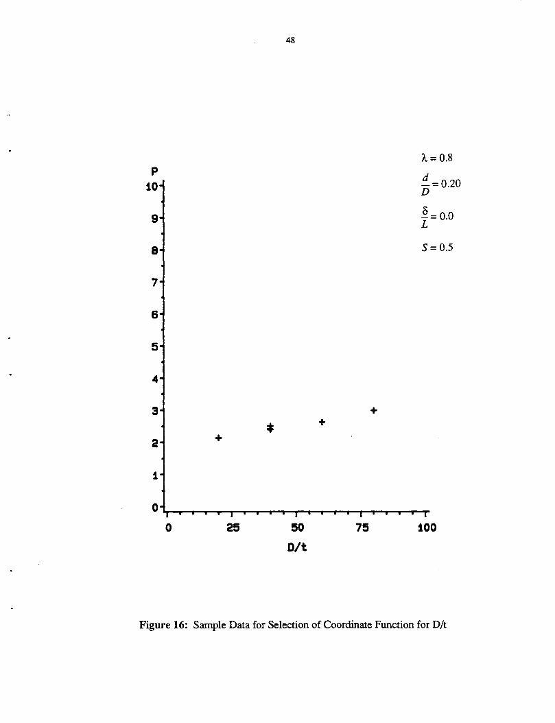
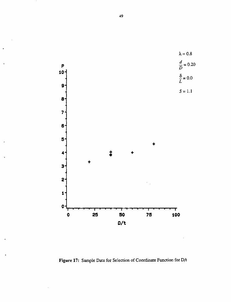
4.2.1.2 Coordinate Function for D/t
Figure 16 shows the nature of the p vs. D/t relationship for A-=0.8, o/L=O.O, d/D=0.20
and S=0.5. Figure 17 is for the same constants except that S=l.l. Examination of these and
other plots of the data resulted in the selection of the simple straight-line coordinate function
H2 = Hv;t= [1 D/tx(lo)-1] (19)
4.2.1.3 Coordinate Function for d/D
The coordinate function for relative dent depth (d/D) is the following simple second
order parabola
H3 = Hd/D = [ 1 (d/D)Zx(10)2] (20)
Examples of p vs. d/D from the database are shown in Figs. 18 and 19 for D/t=40, A-=0.8,
o/L=O.O, with S=0.5 and S=l.l.
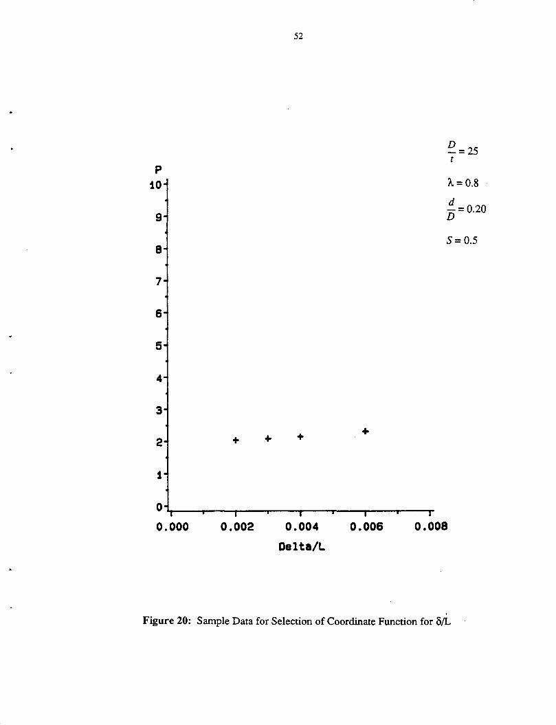
4.2.1.4 Coordinate Function for oiL
The observed relationship between p and o/L appeared to be generally linear. This is
shown in Fig. 20 for D/t=25, A-=0.8, d/D=0.05 and S=0.5, and in Fig. 21 for S=l.l. The
coordinate function selected is a straight line.
H4 = H0;L = [1 o/Lx(10)3 ] (21)
19
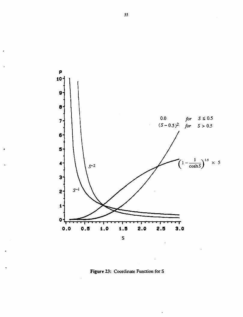
4.2.1.5 Coordinate Function for S
Since, for the column geometries and damage considered, the maximum value of P/P Y
fell over a relatively wide range of values of S, it was difficult to find a linear combination
of functions of S to approximate the load-shortening relationships. The selection of p=P yiP
(as opposed to P!Py) as the response (dependent) variable was made in order to facilitate the
selection of the coordinate function for S .. This is illustrated by considering a fairly typical p
vs. S relationship shown in Fig. 22. The nature of the inverse (P yiP) relationship permitted
the use of separate terms to approximate the descending and ascending portions of the curve.
The following four-term coordinate function was selected for the two ranges of S.
Hs = Hs=
[s-1 s-2 (
1 1 )15 coshS
0]
(1--
1-)1.5 (S-0.5 )2 ]
coshS
(22)
forO~S ~ 0.5
forS>0.5
The individual terms of the coordinate functions for S are plotted in Fig. 23 (note that the
term (1- co:hs) 1.5 is multiplied by a factor of 5.0 for scaling purposes). From this figure it
can be concluded that a linear combination of the terms can produce .. a minimum value of p
over a range of values of S.
20
4.2.2 Formulation of the Regression Model
The coordinate functions are combined in an ordered procedure to form the regression
model as described in Sec. 4.1. The order of the direct product was, as enumerated in
Eq. 15, A., D/t, d/D, o/L, and S. It re!:.ulted in a set of 3x2x2x2x4 = 96 regressors. In
Eq. 23, the computed coefficients (A) of the regressors are given in the form of the transpose
of the rectangular C matrix, cT, (See Sec. 4.1) with Hs (H5) as the remaining free coordinate
function for the relative axial shortening.
91.9227 3.60723 -523.75 333.093
-178.01 -4.1406 1456.72 -694.12
100.402 -0.65395 -1267.9 442.201
-23.015 -0.86287 136.164 -82.801
45.1927 0.940674 -377.91 172.317
-25.81 0.258938 333.524 -110.43
-70.763 -5.392 -418.08 -131.62
132.794 8.44454 479.68 288.668
-69.232 -2.6308 77.1425 -196.13
17.8061 1.3343 101.51 33.0922 (23)
-33.477 -2.0771 -110.61 -72.826
cr = 17.5542 0.627405 -27.334 49.5474
-37.029 -0.28566 409.66.3 -169.59
63.0653 0.999531 -665.13 262.062
-26.079 -0.98045 240.142 -77.67401
9.19786 0.243448 -90.288 38.6192
-15.416 -0.60022 136.913 -55.105
6.09993 0.456124 -38.061 10.5092
23.8209 2.47795 199.192 24.385
-41.639 -4.4515 -356.47 -34.082
18.4614 2.10251 166.031 5.36668
-6.2383 -0.67844 -50.645 -6.8102
10.8385 1.23408 93.3905 8.523461
-4.7286 -0.59913 -46.209 0.0
21
Note that each J'th column of cT contains the coefficients of the reqressors which include the
J'th term of the coordinate function Hs. The zero in cT (the bottom right comer) is the con
sequence of collinearity which resulted from the database used, the selected coordinate func
tions, and the computational precision used by SAS. [7]
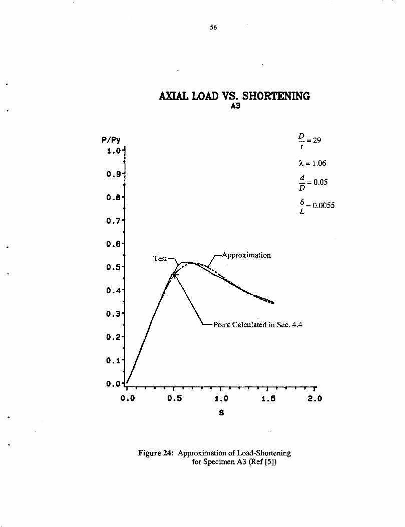
To determine pas a function of S, the C matrix is post-multiplied by Q; which is the
direct product of all coordinate functions except H5 = Hs (See Sec. 4.1). The resultant row
The coefficients, Ar, are calculated from Eq. 14 by post-multiplying matrix C by Q~. (Matrix cT is given in Eq. 23) The resultant four coefficients form a column matrix Ar
shown here as a transpose.
(32)
A;= { 0.932524 0.0134093 6.6042 -Q.66175 }
The p vs. S relationship is then given by Eq. 27. p
where the hs1 to hs4 are defmed in Eq. 22. The approximate load-shortening relationship is
then calculated from Eq. 33 for specific values of S = ~. To further illustrate the calculaLEY
tion of the load-shortening relationship, the load, PIP Y' is determined from Eq. 33 for S=0.5
and the calculated point is indicated in Fig. 24. For S=0.5, the coordinate function Hs is
Hs = [2.0 4.0 0.038077 O.O] (34)
Then, p is given by p
p = 2 = 1.865 + 0.053637 + 0.25147 + 0.0 = 2.170 p
And finally, the nondimensionalized axial load is
p = - 1-= 0.461 py 2.170
(35)
(36)
24
4.5 Range of Applicability The approximation of load-shortening behavior is valid for ranges of column
geometries generally found in fixed offshore platforms. The method is limited by the range
of data in the database used in the regression analysis as indicated in Table 2.
• D/t = 20-80
• A= 0.4 - 1.06
• d/D = 0.05 - 0.30
• 8/L = 0.0- 0.01
In addition, the applicability is limited by the relative damage constraints of Eq. 17.
D - ~ 30 + 233.3 u for A ~ 0.5 + u t
D - ~ 96.67-133.3 A.+ 366.7 u t
for 0.5 + u < A ~ 0.5 + 2.5 u
The range of applicability of the method may be increased as more data become avail
able.
25
5. Summary, Conclusions and Recommendations
5.1 Summary and Conclusions A simplified engineering method was developed to predict the load-shortening
response of damaged (dented and crooked), pin-ended, tubular columns. The method is
based on an analytical model and a regression analysis of data from a fmite element analysis
and published experimental results.
5.1.1 Finite Element Computer Analysis
Since a dented member subjected to an axial load undergoes plastification and large
deformations, it was necessary to use a finite element program which would be capable of
taking these effects into account. The fmite element program ADINA was selected since it
has suitable shell elements for large-displacement analysis ... After considerable experimen
tation, a discretization model that took advantage of the double symmetry of the problem
was developed. The model had 32 shell elements, 4 beam elements ·and 268 nodal points
(1162 degrees of freedom) and gave reasonably good correlation with the experimental
curves in the database. The program was then used to generate load-shortening relationships
to be included in the database to supplement the curves available from previous experimen
tal research.
5.1.2 Database for Axial Behavior of Damaged Compression Members
All experimental data available in published literature on the axial behavior of dented
and crooked tubular members under concentrically applied axial load was collected and put
into a database (Total of 31 curves). Information for each specimen covers the following
items: Source, identification, data on material, geometry, location and amount of damage,
and the load vs. axial shortening relationship with at least 10 points and at least 4 points in
the post-ultimate range. The data can be readily retrieved, manipulated and analyzed with
the SAS software selected for this pwpose. Computer generated results were used to fill in
and supplement the experimental data mainly to cover sparsely populated ranges of
parameters. (A total of 56 curves)
26
5.2 Selection of Parameters The axial load capacity for damaged columns was defmed as a function of five
parameters; D/t, A., diD (relaive dentdepth), o/L (out-of-straightness), and S (average axial
strain divided by yield strain).
5.2.1 Selection of Coordinate Functions
The functional effect of each parameter on the axial behavior was studied by trial-and
error to fmd a simple yet accurate expression to approximate the relationship. Two, three or,
at the most, four-term functions were tried, and the ones with better accuracy selected.
Since the total number of terms in the fmal approximation function would be the product of
the number of terms in all coordinate functions, as few terms as possible were used for the
individual functions. The fmal selection gave a total of 96 terms. It was also necessary to
divide the axial behavior curve into two ranges with different load-deformation coordinate
functions in order to increase the degree of accuracy.
5.2.2 Development of Approximate Engineering Method
The engineering method developed here allows a rapid computation of the load
deformation relationship once the dimensions and material properties (yield stress) and the
amount of damage are known or estimated. The resultant relationship which covers the
elastic pre-ultimate, ultimate and post-ultimate ranges, can be used for practical application
within the ranges of parameters specified. The method requires storage of a set of 96 con
stants and can be readily programmed and used as a subroutine in a larger program for struc
tural analysis of offshore framed structures.
5.2.3 Limitations of the Method
At present, the engineering method, with the coordinate functions used, was found to
be much more accurate for members with significant degree of damage and when D/t is
relatively low, yet in the primary range of practical design (D/t<80). The fmal formulation
of the method is applicable with confidence mainly in the following ranges of parameters:
• D/t = 20-80
• A.= 0.4 - 1.06
• d/D = 0.05 - 0.30
27
• o/L = 0.0- 0.01
with the additional constraints imposed by Eq. 17.
Comparison of the method with the data available showed good correlation as indicated
by the standard deviation of 0.0364 and the root-mean-square of the relative error of 0.0733.
5.3 Recommendations for Future Work Work that can be recommended on the basis of this study can be given in two parts: a
direct extension and completion of the results obtained in this report, and the related topics
which can be viewed as new areas.
5.3.1 Extension of Current Work
The following items can be viewed as a direct supplement and extension of the work
completed and described in this report.
1. Tests on large-scale specimens are needed. ·Since the database contained only test results from small-scale tests and from computer' program which had good correlation with the small-scale tests (thus, representing small-scale tests), there is an urgent need for tests on prototype-sized specimens which would incorporate residual stresses, imperfections, and other characteristics of tubular members as they are encountered in offshore structures. Note that the small-scale specimens were manufactured and stress relieved by annealing, rather than fabricated by cold-rolling and welding. These large-scale tests should include some specimens which, in terms of non-dimensional parameters, duplicate small-scale tests conducted in the past. They should also cover the whole range of parameters of practical interest. For example, D/t=20 to 100.
2. Generation of more data, experimentally or by using a computer program, is needed in order to expand the database for a more thorough study of the behavior and of the influence of the parameters involved.
3. Extension of the approximate method into the range of "peaked" behavior is needed. This is considered to be an elaboration of the work completed in this study.
5.3.2 Further Research on Damaged Tubular Members
Three areas need attention: further work on dented and crooked members, corroded
members, and members with fatigue cracks.
28
5.3.2.1 Dented and Crooked Members
This research should cover the following items:
1. The effect of end eccentricity on the behavior of dented members requires additional experimental and analytical work.
2. End restraints, elastic and inelastic, need consideration; experimental and analytical, possibly by using small-scale specimens.
3. Effect of lateral loading needs to be investigated since members in the splash zone are subjected to heavy wave action.
5.3.2.2 Corroded Members
The effect of corrosion on the behavior of tubular members needs to be investigated.
This should include the effect of loss of member net section as well as the effect of holes
resulting from severe corrosion. Research in this area should address the following items:
1. The establishment of parameters to quantify the amount and location of corrosion damage.
2. The investigation of the effect of corrosion, as defmed by these parameters, on the pre-ultimate, ultimate, and post-ultimate response of the member.
3. The development of an engineering method (simplified procedure) for the behavior of corroded members, possibly, by modifying the method :developed. for dented members. Modified or new coordinate functions will be needed.
5.3.2.3 Members with Fatigue Cracks
There are two main areas of research related to fatigue:
1. Effect of fatigue cracks (size and location) on the short-term axial load-deformation behavior of tubular members. This study is closely related to the subject of this report and would follow a similar procedure.
2. Initiation and growth of fatigue cracks. Consideration of load spectra, structural details, presence of salt water and the wetting cycle would be the areas of work. Of particular interest is the effect of corrosion notching on fatigue life.
29
Acknowledgments This research was sponsored by the Minerals Management Service of the U.S. Depart
ment of the Interior (Contract No. 14-12-0001-30288) and the American Iron and Steel In
stitute (AISI Project 338) under the DOI/AISI Cooperative Research Program. The authors
are grateful for this support and for the advice and guidance given by the members of the
project Task Force; C.E. Smith and A. C. Kuentz, the respective representatives of the spon
soring institutions, and R.H. Wildt (Chairman of the Task Force) of Bethlehem Steel Cor
poration, C. Capanoglu of Earl and Wright, C.D. Miller of CBI Industries, Inc.,
J. de Oliveira and F. Botros of Conoco, Inc., and J.B. Gregory of the Minerals Management
Figure 24: Approximation of Load-Shortening for Specimen A3 (Ref [5])
2.0
P/Py 1.0
0.9
0.8
0.7
0.6
0.5
0.4
0.3
0.2
0.1
0.0
0.0
57
AXIAL LOAD VS. SHORTENING 83
0.5 1.0 1.5
s
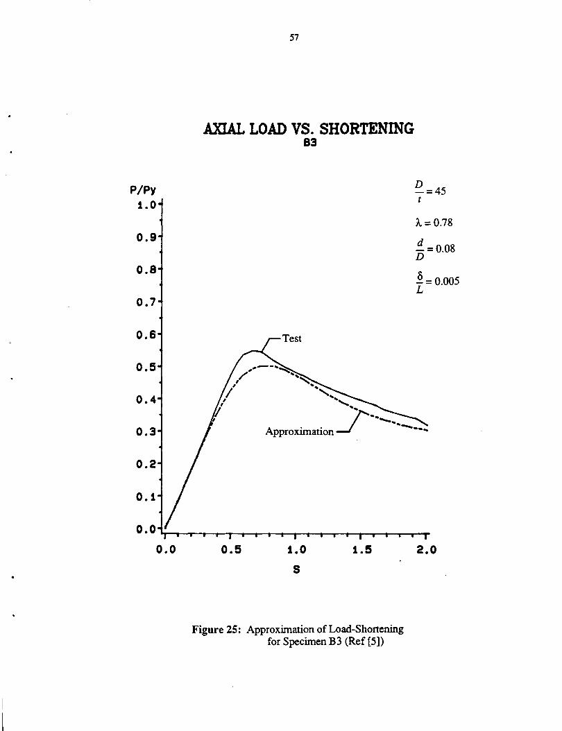
Figure 25: Approximation of Load-Shortening for Specimen B3 (Ref [5])
D -=45 t
A.= 0.78
d -=0.08 D
0 -= 0.005 L
2.0
P/Py 1.0
0.9
0.8
0.7
0.6
0.5
0.4
0.3
0.2
0.1
0.0
58
AXIAL LOAD VS. SHORTENING A1A
............. r-Approximation ,' .. ,(
0.5
.. ,
1.0
s
.... ' .. .. ~
1.5
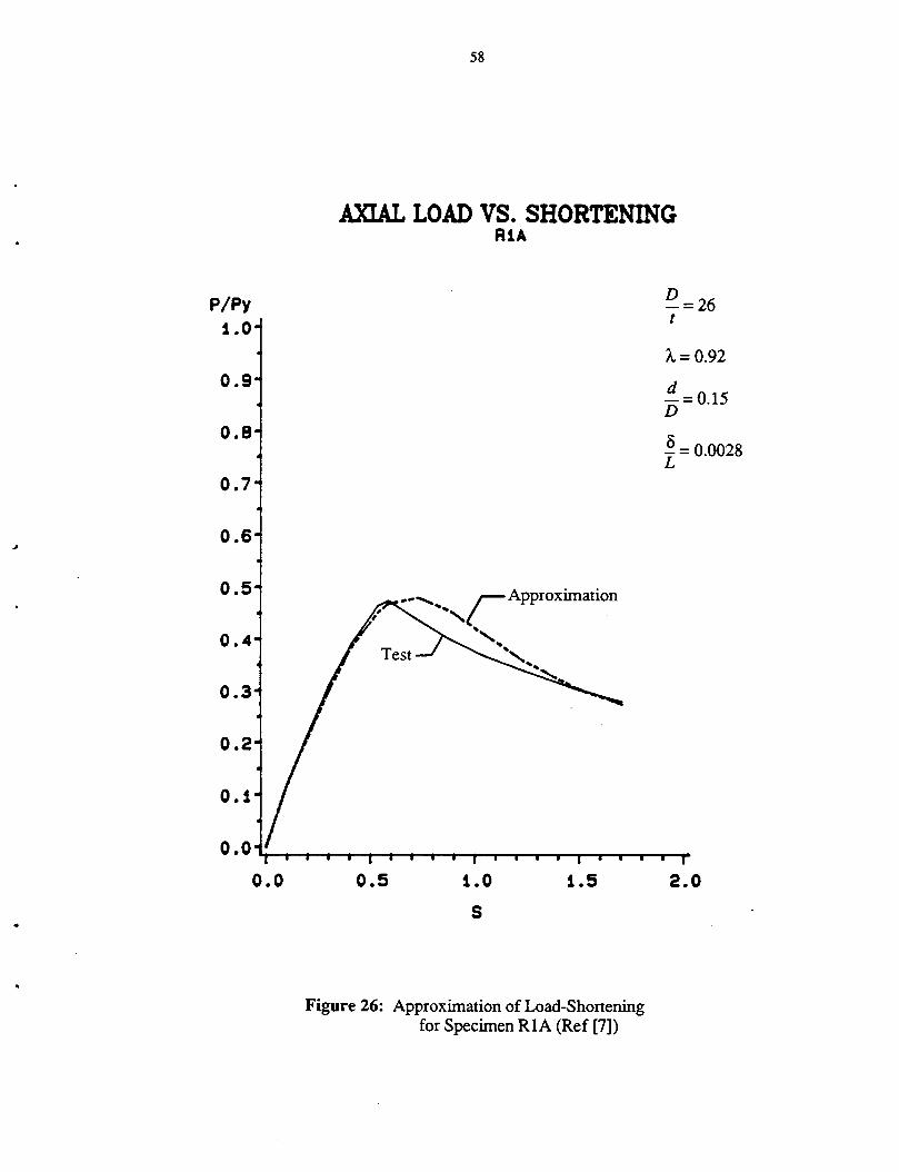
Figure 26: Approximation of Load-Shortening for Specimen RlA (Ref [7])
D -=26 t
A.= 0.92
d D = 0.15
0 -= 0.0028 L
2.0
P/Py 1.0
0.9
0.8
0.7
0.6
0.5
0.4
0.3
0.2
0.1
0.0
59
AXIAL LOAD VS. SHORTENING IIICII
D -=41 t
A.= 0.62
d -=0.10 D
0 -= 0.0018 L
.... '""" .. ......;--Approximation ....
0.5 1.0
s
' .. .. , .... ' .. ...
1.5
Figure 27: Approximation of Load-Shortening for Specimen illCII (Ref [9])
2.0
P/Py 1.0
0.9
0.8
0.7
0.6
0.5
0.4
0.3
0.2
0.1
0.0
0.0
60
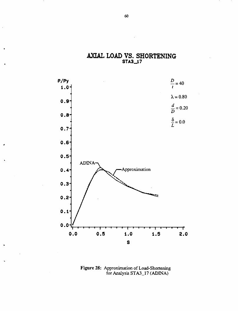
AXIAL LOAD VS. SHORTENING STA3J7
0.5
~rApproxirnation
"'~ "' ...
1.0
s 1.5
D -=40 t
'A= 0.80
d -=0.20 D
o_ --0.0 L
2.0
Figure 28: Approximation of Load-Shortening for Analysis ST A3_17 (ADINA)
P/Py 1.0
0.9
0.8
0.7
0.6
0.5
0.4
0.3
0.2
0.1
0.0
0.0
61
AXIAL LOAD VS. SHORTENING STA3.J56
D -=30 t
A.= 0.94
d D = 0.10
0 I= 0.01
.. rpprox.imation
0.5 1.0 1.5 2.0
s
Figure 29: Approximation of Load-Shortening for Analysis STA3_56 (ADINA)
>I
62
Appendix A Nomenclature
A
A. l
Ar
B
c D
d
E
H
hij
1
J k
L
ld
1
m
~
n
p
py
p
Q
Qe
Qr
'li R
Rd
Column Matrix of Regression Coefficients
Column Matrix of Regression Coefficients for the z1h Coordinate Function
Column Matrix of a Reduced Set of Regression Coefficients
Matrix of Regressors for Given Values of hidependent Variables
Rectangular Matrix of Regression Coefficients
Diameter to Mid-thickness
Dent Depth
Modulus of Elasticity
Coordinate Function (Row Matrix)
The ;1h Term of the zth Coordinate Function
Counter for Data Points
Counter for Regressors and Terms of Coordinate Functions
Counter for hidependent Variables
Length of Column
Length of Dent
Number of Data Points
Number of Regressors
Number of Terms in the zth Coordinate Function
Number of hidependent Variables
Axial Load
Squash Load= 1tD tcry p
Nondimensionalized hiverse Axial Load= ;
Row Matrix of Regressors
Row Matrix Formed by Direct Product of Coordinate Functions To Be Eliminated
Row Matrix Formed by Direct Product of a Reduced Set of Coordinate Functions
The ith Regressor
Radius to Mid-thickness
Radius to Dent (See Fig. 3)
r
s
t
u
X
z
63
Radius of Gyration
Relative Shortening of Column, S = ~ LEY
Thickness of Tube Wall
Damage Factor=~+ 35~
Longitudinal Coordinate Measured from Mid-length
Lateral Deflection (Initial Crookedness) as a Function of x
Axial Shortening of Column
Maximum Initial Crookedness
Strain cr
Yield Strain, S = ;
L _r- .. _Slenderness Parameter, A. = -"~f.....
Ttr -y
Stress
Yield Stress
Angle as Defmed in Fig. 3
Dent Depth as a Function of Its Length and Distance x
64
. References
[1] Ellinas, C.P. illtimate Strength of Damaged Tubular Bracing Members. ASCE Journal of Structural Engineering 110(2):245-259, February, 1984.
[2] Moan, T. Advances in the Design of Offshore Structures for Damage- Tolerance. In Smith, C.S. and Clarke, J.D. (editor), Advances in Marine Structures, pages
472-496. Elsevier Applied Science, London and New York, May, 1986. Proceedings of an International Conference held at the Admiralty Research Establis
ment, Dumferline, 20-23 May 1986.
[3] Ostapenko, A., and Surahman, A. Structural Element Models for Hull Strength Analysis. Fritz Engineering Laboratory Report No. 480.6, Lehigh University, September,
1982.
[4] Ostapenko, A., Surahman, A. Axial Behavior of Longitudinally Stiffened Plates. In Stability of Metal Structures- Preliminary Report, pages 291-303. CTICM, Paris,
November, 1983. (Paris Session, November 16-17, 1983).
[5] Ostapenko, A. Computational Model for Load-Shortening of Plates. In Proceedings of Structural Stability Research Council, pages 167-182. Structural
Stability Research Council, 1985.
[6] Padula, J.A., and Ostapenko, A. Indentation Behavior of Tubular Members. Fritz Engineering Laboratory Report No. 508.8, Lehigh University, Bethlehem, PA,
June, 1988.
[7] SAS User's Guide: Statistics Version 5 edition, SAS Institute, Cary, N.C., 1985.
[8] Smith, C.S., Kirkwood, W. and Swan, J.W. Buckling Strength and Post-Collapse Behaviour of Tubular Bracing Members In
cluding Damage Effect. In Stephens, H.S. (editor), Proceedings of the Second International Conference on
the Behavior of Off-Shore Structures, pages 303-326. BHRA Fluid Engineering, London, England, August, 1979.
[9] Smith, C.S., Somerville, W.L. and Swan, J.W. Residual Strength and Stiffness of Damaged Steel Bracing Members. In Proceedings of the 13th Offshore Technology Conference, pages 273-282. Off
shore Technology Conference, Houston, May, 1981. (Paper OTC 3981 ).
65
[10] Smith, C.S. Assessment of Damage in Offshore Steel Platforms. In Proceedings of International Conference on Marine Safety, pages 279-307. ,
Glasgow, England, September, 1983.
[11] Taby, J., and Rashed, S.M.H. Experimental Investigation of the Behaviour of Damaged Tubular Members. Technical Report MK/R92, Department of Naval Architecture and Marine Engineer
ing, The Norwegian Institute of Technology, Trondheim, Norway, 1980.
[12] Taby, J., Moan, T., and Rashed, S.M.H. Theoretical and Experimental Study of the Behaviour of Damaged Tubular Members
in Offshore Structures. Norwegian Maritime Research 9(2):26-33, 1981.
[13] Taby, J., and Moan, T. Collapse and Residual Strength of Damaged Tubular Members. Behaviour of Offshore Structures. Elsevier Science Publishers B.V., Amsterdam, 1985, pages 395-408.
[14] Taby, J. Experiments with Damaged Tubulars. Technical Report 6.07, SINTEF, Norwegian Institute of Technology, Trondheim,
Norway, October, 1986.
[15] Taby, J. Residual Strength of Damaged Tubulars. Final Report 6.10, SINTEF, Norwegian Institute of Technology, Trondheim, Nor
way, October, 1986.
[16] Taby, J. DENTA User's Manual (VAX Version). Technical Report MK/R 93/86, Department of Marine Technology, The Norwegian
Institute of Technology, Trondheim, Norway, November, 1986.
[17] Wierzbicki, T., and Suh, M.S. Denting Analysis ofTubes Under Combined Loading. Technical Report MITSG 86-5, MIT Sea Grant College Program, Massachusetts In
stitute of Technology, 77 Massachusetts Ave., Cambridge, MA 02139, March, 1986.