Shock and Vibration 12 (2005) 177–195 177IOS Press
Axial vibration confinement innonhomogenous rods
S. Chouraa, S. EL-Borgia and A.H. Nayfehb,∗aApplied Mechanics and Systems Research Laboratory, Tunisia Polytechnic School, B.P. 743, La Marsa 2078,TunisiabDepartment of Engineering Science and Mechanics, MC 0219, Virginia Polytechnic and State University,Blacksburg, VA 24061, USA
Received 16 January 2004
Revised 20 August 2004
Abstract. A design methodology for the vibration confinement of axial vibrations in nonhomogenous rods is proposed. This isachieved by a proper selection of a set of spatially dependent functions characterizing the rod material and geometric properties.Conditions for selecting such properties are established by constructing positive Lyapunov functions whose derivative with respectto the space variable is negative. It is shown that varying the shape of the rod alone is sufficient to confine the vibratory motion.In such a case, the vibration confinement requires that the eigenfunctions be exponentially decaying functions of space, wherethe notion of spatial domain stability is introduced as a concept dual to that of the time domain stability. It is also shown thatvibration confinement can be produced if the rod density and/or stiffness are varied with respect to the space variable while thecross-section area is kept constant. Several case studies, supporting the developed conditions imposed on the spatially dependentfunctions for vibration confinement in vibrating rods, are discussed. Because variation in the geometric and material propertiesmight decrease the critical buckling loads, we also discuss the buckling problem.
Keywords: Axial vibration, vibration confinement, material and geometric properties, buckling
1. Introduction
Flexible structures, such as aerospace and ship structures, large communication antennas, and seismically excitedbuildings and bridges, are exposed to vibration due to various external and/or internal excitations. They often exciteunwanted structural resonances, which can cause damage or transmission of vibrational energy to distant parts orregions where they cannot be tolerated. Therefore, it may be of interest to remove the vibrational energy fromthe more sensitive parts of the structure and transfer it to the less sensitive parts. The sensitive parts of flexiblestructures are defined to be a set of spatial regions in which vibrations must be eliminated to ensure a better structuralperformance and less chances of destructing these structures. The sensitive parts include end-effectors of flexiblerobot manipulators.
Allaei investigated the feasibility of developing an efficient vibration-control methodology based on mode local-ization and termed it as vibration control by confinement [1]. The advantage of the confinement approach over con-ventional control in isolating the sensitive parts of a structure was demonstrated with several examples by Allaei [2].The eigenvector assignment has been demonstrated to be an efficient tool for vibration control [3,19,22]. It is ameans of redistributing the vibrational energy in the structure, and thus allowing the sensitive parts to converge totheir steady-state values at fast rates.
178 S. Choura et al. / Axial vibration confinement in nonhomogenous rods
The eigenstructure assignment procedure has found application in a wide variety of control problems, such asthose associated with flight-control design [13,21] and the control of vibrating structures [15]. An extensive literatureis concerned with the development of algorithms for the computation of feedback gains that yield a desired set ofclosed-loop eigenvalues and eigenvectors [9–11,15,23].
Another design technique known as ‘Inverse Eigenvalue Problem’ arises in control-system design, system identifi-cation, structural analysis, mechanical system simulation, etc. . . The essential idea of an inverse eigenvalue problemis to reconstruct a matrix from prescribed spectral data, which may consist of the complete or only partial informationof the eigenvalues or eigenvectors [7]. The objective of an inverse eigenvalue problem is to construct a matrix thatmaintains a specific structure and satisfies given spectral properties. Ram and Elhay have presented a method thatconstructs tridiagonal symmetric quadratic damping and stiffness matrices based on a given set of eigenvalues [17].Sivan and Ram have treated the problem of determining structural alteration from a given set of eigenvalues andeigenvectors in the presence of model uncertainties [20]. Ram has synthesized control forces for shifting somepoles of a vibrating rod to prescribed locations while keeping the other poles unchanged [16]. Ram and Elhay havereconstructed the shape of a rod with varying cross-section [18]. Their reconstruction is based on a discretized modelof the rod leading to a specially structured matrix pencil.
Recently, Choura and Yigit have developed a strategy for the confinement of vibrations in flexible structures bydistributed actuators [5]. The strategy consists of altering the original mode shapes of a flexible structure usingfeedback. The altered mode shapes are exponentially decaying functions of space that nearly vanish at the structuralregion where the vibrational energy is to be removed and transferred to the remaining parts. They have shownthat it is possible to use an equivalent set of discrete actuators for confining the vibration [24]. The concept ofusing a reduced number of point actuators has been treated in [6]. As compared to the procedure of eigenstructureassignment offered by Shaw and Jayasuriya [19] and Song and Jayasuriya [22], Choura has developed a detailedassignment procedure for the purpose of vibration confinement [3]. Feedback forces have been used to allow parts ofa structure reach their equilibria at fast rates at the expense of slowing down the convergence of the remaining partsto zero. The control strategy has been used to investigate the confinement and suppression of vibrations resultingfrom an initial energy distribution using feedback forces whose number is equal to that of the dimension of thediscretized model. The strategy of vibration confinement by passive means has been applied to seismically excitedstructures [4].
In this paper, we consider the reconstruction (for existing structures) or design (for new structures) of rodswith spatially varying shape and material properties by a proper selection of their cross-sectional areas, theirmodulii of elasticity, and/or their densities. The key idea of such a selection is to setup the ordinary-differentialequation associated with the eigenfunctions as a space-domain stability problem dual to that of time-domain stability.Therefore, design techniques, such as pole placement and Lyapunov energy functions, can be used to determine thenecessary conditions for assigning the spatially varying shape and material properties of the vibrating rod.
2. Problem formulation
Consider the axial vibration of a rod, shown in Fig. 1, with variable cross-sectional area A (x), variable Young’smodulus of elasticity, E (x) and variable mass density per unit length ρ (x), and governed by
∂
∂x
[E (x)A (x)
∂u
∂x
]− ρ (x)A (x)
∂2u
∂t2= 0 (1)
where the neutral axis is assumed to be linear.It is known that the vibratory energy is equally distributed over the spatial domain of a rod having constant
cross-section and constant material properties. One way to redistribute the energy in such a rod is to apply activecontrol employing distributed force actuators [5] or point force actuators [24]. This paper proposes an alternate wayfor the redistribution of energy by modifying the rod’s geometric and material properties. From a practical pointof view, the designer is allowed to modify an already existing rod by adding and/or removing material. Therefore,the objective of this study is to determine a set of functions A (x), E (x), and ρ (x) such that the rod preserves alocalization or confinement behavior during its vibrational motion in which certain parts of the rod will experiencelower vibration amplitudes.
S. Choura et al. / Axial vibration confinement in nonhomogenous rods 179
( ) ( ) ( )xExAx , ,ρ
L x
Neutral Axis
Fig. 1. Rod with variables cross section and variable material properties.
The axial displacement is expressed in the following form:
u (x, t) = U (x) ejω t (2)
where U (x) is the eigenfunction, ω is the natural frequency of axial vibration, and t is the time variable. SubstitutingEq. (2) into Eq. (1) yields
d
dx
[E (x) A (x)
dU (x)dx
]+ ω2ρ (x) A (x) U (x) = 0 (3)
Vibration confinement can be defined as reducing the absolute value of U (x) in the sensitive parts; that is,
|U (x)| < ε for ∀x ∈ D1∪D2 . . . ∪ Dn (4)
where ε is a small positive constant and the Di, i = 1,2,. . . ,n correspond to the spatial intervals associated with theparts that are sensitive to vibration.
The strategy for vibration confinement proposed in this study converts the eigenfunctions of the original structureinto exponentially decaying functions of the spatial coordinate x. If the size of the structure is large (i.e., thedimension of the rod’s length L is large), then spatial confinement of vibration becomes dual to time domain stability.It is, therefore, possible to design the functions A (x), E (x), and ρ (x) in Eq. (3) utilizing the classical poleplacement techniques, such as using the Routh-Hurwitz criterion or the Lyapunov stability technique, and applyingthem to the spatial domain. In particular, the coefficients in Eq. (3) must be properly selected in order to “stabilize”the spatial dynamics, where the concept of spatial domain stability is introduced as a concept dual to that of thetime-domain stability. Next, a strategy for selecting the above functions is developed for the general case followedby particular cases.
3. Conditions for vibration confinement
Consider the axial vibration of bars in which the cross-section area A = A (x), Young’s modulus of elasticityE = E (x), and mass density per unit length ρ = ρ (x) are all taken as variables. In this case, Eq. (3) can berewritten as
[p (x)U ′]′ + ω2 q (x)p (x)
U = 0 (5)
where p (x) and q (x) are positive functions for all x and given by
p (x) = E (x) A (x) q (x) = ρ (x) E (x) A2 (x) (6)
In order to “stabilize” the spatial dynamics, a set of functions A (x),E (x), and ρ (x) can be found using thefollowing candidate Lyapunov function:
V (x) = U2 +1
ω2q (x)[p (x) U ′]2 > 0 (7)
180 S. Choura et al. / Axial vibration confinement in nonhomogenous rods
Using Eq. (5), we simplify the derivative of V (x) with respect to x to
V ′ (x) = − q′ (x)ω2q (x)
[p (x) U ′]2 (8)
which implies that
q′ (x) = [ρ′ (x) E (x) + ρ (x) E′ (x)] A2 (x) + 2ρ (x) E (x) A (x) A′ (x) > 0 (9)
Equation (9) regulates the choice of the rod parameters and provides a relationship among them. It provides condi-tions on the choice of the physical and geometric parameters that lead to vibration confinement in the neighborhoodof x = 0. Conditions on these parameters for vibration confinement at an arbitrary point in the spatial domain aregiven later in this paper. From Eq. (9), it follows that the following cases are possible:
a. keep both of the cross-section area and the density constant across the rod and vary the modulus of elasticityprovided that its spatial derivative with respect to x is positive for all x. This implies that the rod stiffnessincreases and becomes larger in the neighborhood of the right end,
b. keep both of the cross-section area and the modulus of elasticity constant across the rod and vary the rod densityprovided that its spatial derivative with respect to x is positive for all x. This implies that the rod densityincreases and becomes larger in the neighborhood of the right end,
c. keep the cross-section area constant across the rod and vary both of the modulus of elasticity and the densityprovided that the spatial derivative of their product with respect to x is positive for all x. This implies thatboth of the rod stiffness and density increase simultaneously or one of them decreases and the other increasesmore rapidly. This is the case of a Functionally Graded Material (FGM), which is essentially a two-phasenonhomogeneous particulate composites synthesized in such a way that the volume fractions of the constituentmaterials, such as ceramic and metal, vary continuously along a spatial direction to give a predeterminedcomposition profile, resulting in a relatively smooth variation of the mechanical properties [8].
Because variations in the geometric and material properties might decrease the critical buckling loads, weinvestigate the effect of the distributed geometric and physical properties on the buckling of a fixed-fixed rod. For aconstant axial load, the static buckling problem associated with the rod is described by
d2
dx2
(E (x) I (x)
d2w
dx2
)+ P
d2w
dx2= 0 w (0) = w (L) = 0;
dw
dx(0) =
dw
dx(L) = 0 (10)
It follows from this boundary-value problem that only the modulus of elasticity and the second moment of areaaffect the buckling load P . The absence of the mass density shows that the cross-section area and the modulus ofelasticity can be designed first to satisfy certain design conditions for the buckling problem. The mass density canthen be designed to compensate for the confinement problem. This is demonstrated through a study case discussedlater in this paper. Next, we give some examples of rods with spatially varying geometric and/or physical propertiesthat demonstrate the validity of condition Eq. (9) and we also address the buckling problem for each example.
We first consider axial vibrations of a rod of length L with variable cross-section area and constant physicalproperties; that is, E (x) = E0 and ρ (x) = ρ0. In this case, we search for possible forms of the cross-section thatallow confinement of vibrations in preferred regions of the rod when the material properties are kept constant. Inthis case, Eq. (9) reduces to
q′ (x) = 2ρ E A (x) A′ (x) > 0 (11)
which requires the cross-section area to be an increasing function of space over the domain 0 < x < L.
4. An exponentially varying cross-section area
In this case, the cross-section area is distributed according to the following exponential function:
A (x) = A0eαx A (0) = A0 and A (L) = AL (12)
S. Choura et al. / Axial vibration confinement in nonhomogenous rods 181
where α = 1L ln
(AL
A0
). It follows from Eq. (12) that the area increases as the spatial variable x increases. It can be
shown that Eq. (3) simplifies to
U ′′ + α U ′ +ρ0
E0ω2 U = 0 (13)
which in turn yields the characteristic equation
λ2 + αλ +ρ0
E0ω2 = 0 (14)
Thus, the general solution is given by:
U (x) = C1 eλ1x + C2 eλ2x (15)
λ1,2 = −12α ±
√14α2 − ρ0ω2
E0(16)
Next, we consider the cases of fixed-fixed and fixed-free rods, starting with the first.For a fixed-fixed rod, the boundary conditions are given by u (0 , t) = 0 and u (L , t) = 0, and the normalized
eigenfunctions are given by
Um (x) =
√eαL (α3L2 + 4αm2π2)
2 (eαL − 1) m2π2e−
12 αxsin
(mπ
Lx)
(17)
The scalar α must satisfy 0 < α < 2√
ρ0E0
ω1 and the natural frequencies are given by
ω2m =
E0
ρ0
[m2π2
L2+
14α2
], m = 1, 2,3,. . . (18)
For a fixed-free rod, the boundary conditions are u (0 , t) = 0 and u ′ (L , t) = 0. The solution of equation(13) that satisfies the boundary condition u (0 , t) = 0 is given by
Um (x) = Cme−12 αxsin (ηx) (19)
where
η =
√ρ0ω2
m
E0− 1
4α2 (20)
Imposing the boundary condition u ′(L, t) = 0 yields the characteristic equation
cot(ηL) =α
2η(21)
Equation (21) does not have a closed-form solution and, therefore, either numerical or asymptotic methods areneeded for approximating the natural frequencies. The large roots of the characteristic equation can be obtainedusing asymptotic methods as follows. When η is large, the right-hand side of Eq. (21) can be neglected and hencewe obtain cot (ηL) = 0 whose solution is given by
ηL =(
m +12
)π (22)
where m is an integer. Then the solution of Eq. (21) can be sought in the form
ηL =(
m +12
)π + δ (23)
Substituting Eq. (23) into Eq. (21) yields
cot
[(m +
12
)π + δ
]=
αL
(2m + 1)π + 2δ(24)
182 S. Choura et al. / Axial vibration confinement in nonhomogenous rods
Using trigonometric identities, we rewrite Eq. (24) as
cot[(
m + 12
)π]− tan (δ)
1 + tan (δ) cot[(
m + 12
)π] =
αL
(2m + 1)π + 2δ(25)
or
− tan (δ) =αL
(2m + 1)π + 2δ(26)
For small δ, Eq. (26) yields
δ = − αL
(2m + 1)π(27)
Therefore, to the second approximation,
ηL =(
m +12
)π − αL
(2m + 1)π(28)
Substituting Eq. (28) into Eq. (20), we obtain, to the second approximation, the natural frequencies
ρ0ω2m
E0=
12α2 +
1L2
[(m +
12
)π − αL
(2m + 1)π
]2(29)
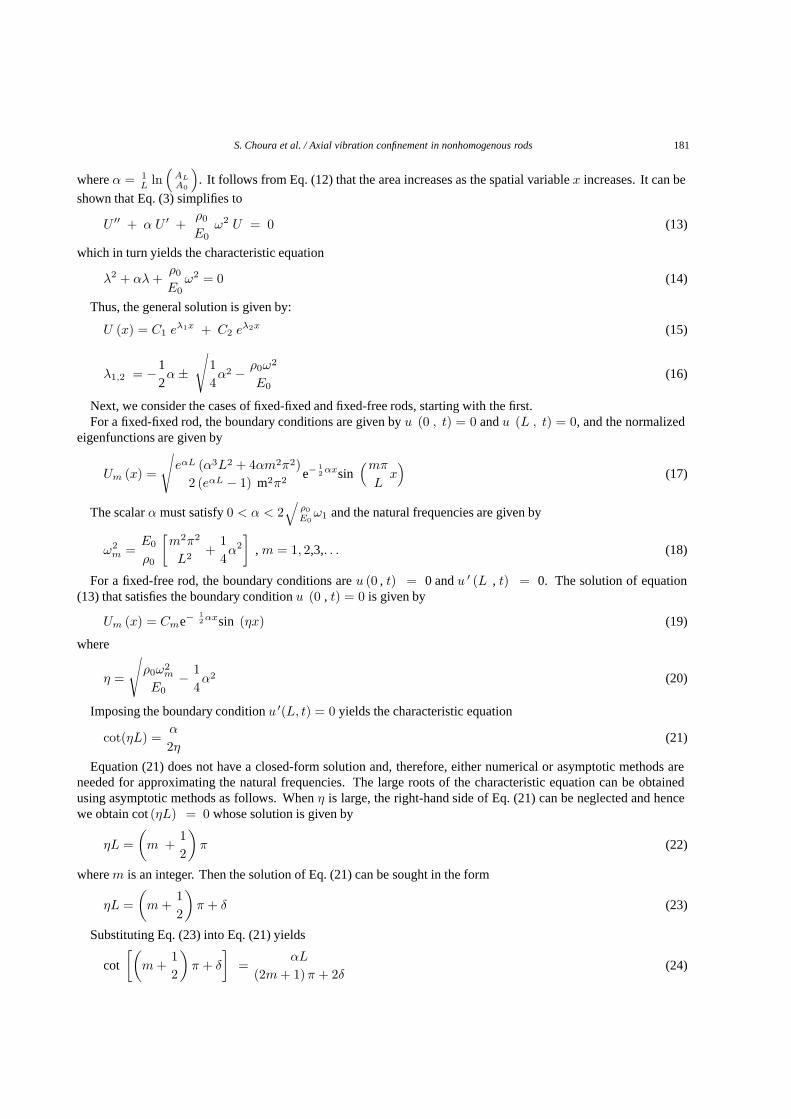
Equation (19) shows that the mode shapes are exponentially decaying functions of the spatial variable x. Highervalues of α lead to faster decay of these eigenfunctions, and therefore a better confinement of the vibrational energyin the neighborhood of x = 0. Figure 2 shows the first three modes and time response to an initial time velocitydistribution with constant physical and geometric properties of a 10-meter aluminum rod (E = 1.5 × 10 6 N / m2,ρ = 8760 kg, and A = 0.01322 m2). Clearly, the vibratory energy is distributed throughout the rod at all times.Figures 3 and 4 show the shape of a square cross-section area, the first three eigenfunctions, and the time response toan initial time velocity distribution for fixed-fixed and fixed-free 10-meter aluminum rods (E 0 = 1.5 × 10⁶ N / m2,ρ0 = 8760 kg, A0 = 10−4 m2, AL = 9 × 10⁻² m2 and α = 0.68). As expected, the vibratory motion isconfined in the left region of the rod. We note that the frequencies shown in figure 4 correspond to the exact values.The first three approximate frequencies obtained from Eq. (29) are, respectively, 6.8605, 10.6816, and 14.6745,which are close to the exact values.
Next, we address the buckling problem; the second moment of area is given by I (x) = I 0e2αx. Hence, Eq. (10)
becomes
d2
dx2
(e2αx d2w
dx2
)+ κ2 d2w
dx2= 0 w (0) = w (L) = 0;
dw
dx(0) =
dw
dx(L) = 0 (30)
where κ2 = PE0I0
and I=0
A20
12 . The general solution of Eq. (30) can be expressed as
w (x) = C1 + C2x + C3J0
(κ
αe−αx
)+ C4Y0
(κ
αe−αx
)(31)
where Jn and Yn are the Bessel functions of the first and second kinds of order n, respectively. Applying theboundary conditions and using Mathematica, we find that the characteristic equation leads to the following lowestfive critical axial loads: P1 = 20.5E0I0, P2 = 39.1E0I0, P3 = 77.8 E0I0, P4 = 114.2E0I0, and P5 = 171.9E0I0.
For comparison purposes, we investigate the buckling problem associated with a 10-meter aluminum rod havingconstant physical and geometric properties (E (x) = E0 and I (x) = 17466I0) where the second moment of areais calculated by assuming that the material volumes of both rods are the same. For the uniform beam, the bucklingproblem is given by
d4w
dx4+ κ2 d2w
dx2= 0; w (0) = w (L) = 0;
dw
dx(0) =
dw
dx(L) = 0 (32)
The general solution of Eq. (32) can be expressed as
w (x) = C1 + C2x + C3 cos (κ x) + C4 sin (κ x) (33)
S. Choura et al. / Axial vibration confinement in nonhomogenous rods 183
0 2 4 6 8 10-1
-0.5
0
0.5
1
w1=4.110 2 4 6 8 10
-1
-0.5
0
0.5
1
w2=8.22
0 2 4 6 8 10-1
-0.5
0
0.5
1
w3=12.33
0 2
4 6
8 10 0
2
4
6
8
10
-0.0002
0
0.0002
0 2
4 6
8 10 x
u(x,t) t
Fig. 2. First three eigenfunctions and time response of an aluminum fixed-fixed rod.
Applying the boundary conditions, we obtain the characteristic equation
κL sin(κL) + 2 cos(κL) = 2 (34)
Using asymptotic methods, we find that the large roots of Eq. (34) are given by
κL = nπ +2[1 − cos (nπ)]
nπcos (nπ)for n � 2 (35)
The lowest five exact and approximate roots are:Exact roots: κL =6.2832, 8.9868, 12.5664, 15.4505, and 18.8496Approximate roots: κL =6.2832, 9.0004, 12.5664, 15.4533, and 18.8496
We note that the roots in Eq. (35) corresponding to even values of n are exact and those corresponding to oddvalues of n are approximate. The lowest five critical buckling loads obtained numerically as well as from theasymptotic solution are:
Comparison of the set of critical axial loads associated with a rod having spatially varying cross-section areawith the above values reveals that the first critical value is decreased remarkably. This constitutes a disadvantagein the sense that improving vibration confinement results in a weak rod resistance to buckling in case the materialvolume is kept the same for both rods. This observation is valid only for rods having constant material propertiesand variable geometric properties. On the other hand, if the cross-section area is kept at the smallest value associatedwith the spatially varying rod A0, then the first five critical axial loads become: P1 = 0.81E0I0, P2 = 2.39E0I0,P3 = 4.76E0I0, P4 = 7.91E0I0, and P5 = 11.86E0I0. In such a case, varying the cross-section area improvessimultaneously the confinement of vibration and the rod resistance to buckling.
In order to avoid the decrease in the critical buckling loads, we investigate possibilities of varying the materialproperties with or without varying the geometric properties. This is discussed thoroughly in Sections 6–8.
5. Linearly varying cross-section area
For generally varying cross-section areas,
S. Choura et al. / Axial vibration confinement in nonhomogenous rods 185
0 5 10-0.2
-0.1
0
0.1
0.2
x
beam
sha
pe
0 5 100
0.1
0.2
0.3
0.4
0.5
x
Firs
t m
ode
shap
e
0 5 10-0.2
0
0.2
0.4
0.6
x
Sec
ond
mod
e sh
ape
0 5 10-0.2
0
0.2
0.4
0.6
0.8
x
Third
mod
e sh
ape
0 2
4 6
8 10 0
0.5
1
1.5
0 0.00025 0.0005
0.00075
0 2
4 6
8 10 x
u(x,t) t
7.26=1ω
10.81=2ω 14.65=3ω
Fig. 4. Shape, first three eigenfunctions and time response of an aluminum fixed-free rod.
A (x) = A0e
∫ x
0f(σ)dσ (36)
and Eq. (3) takes the form
U ′′ + f (x) U ′ +ρ0
E0ω2 U = 0 (37)
According to the spatial stability condition given in Eq. (11), the function f (x) must be positive for all x. Thiscondition implies that the cross-section is monotonically increasing function of x.
Next, we consider the case of linearly varying cross-section areas; that is,A (x) = A0 + (AL−A0)
L x corresponding to f (x) = AL−A0A0L+(AL−A0)x
, where AL > A0 and α = AL−A0LA0
.In this case, the rod is stiffer in the vicinity of the right end. Then, the solution of Eq. (37) that vanishes at the left
end is given by
Ui (x) = Ci
[J0
(√ρE
ωi
α (1 + αx))
J0
(√ρE
ωi
α
) − Y0
(√ρE
ωi
α (1 + αx))
Y0
(√ρE
ωi
α
)]
i = 1, 2, 3, . . . (38)
Then the corresponding characteristic equation is
J0
(√ρ
E
ωi
α(1 + αL)
)Y0
(√ρ
E
ωi
α
)− J0
(√ρ
E
ωi
α
)Y0
(√ρ
E
ωi
α
)(1 + αL) = 0 (39)
186 S. Choura et al. / Axial vibration confinement in nonhomogenous rods
0 2 4 6 8 10-0.5
0
0.5
Beam Shape
0 2 4 6 8 100
0.2
0.4
0.6
0.8
1
w1=3.48
0 2 4 6 8 10-0.5
0
0.5
1
w2=7.60
0 2 4 6 8 10-0.5
0
0.5
1
w3=11.73
0 2 4 6 8 10-0.5
0
0.5
1
w4=15.86
0 2 4 6 8 10-0.5
0
0.5
1
w5=19.98
0 2
4 6
8 10 0
1
2
3
-0.0002
0
0.0002
0 2
4 6
8 10 x
u(x,t) t
Fig. 5. Shape, first five eigenfunctions, and time response of an aluminum fixed-fixed rod with a linearly increasing area.
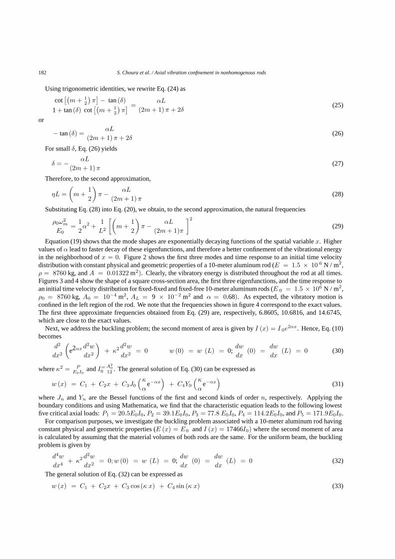
Figure 5 shows the rod shape and the first five eigenfunctions for (E 0 = 1.5 106 N / m2, ρ0 = 8760 kg,A0 = 10−4 m2, and AL = 9 10−2 m2). The time response of the aluminum rod for an initial time velocitydistribution, shown in the same figure, depicts that the vibrations are confined towards the left end (x = 0).
In this case, the associated buckling problem is given by
d2
dx2
[(1 + αx)2
d2w
dx2
]+ κ2 d2w
dx2= 0 w (0) = w (L) = 0;
dw
dx(0) =
dw
dx(L) = 0 (40)
The general solution of Eq. (40) can be expressed as
w (x)=C1+C2x+√
1 + αx
(C3cos
[√4κ2 − α2ln (1 + αx)
2α
]+C4sin
[√4κ2 − α2ln (1 + αx)
2α
])(41)
Applying the boundary conditions to Eq. (41) yields the characteristic equation
L(2κ2 − α2
)sin
[√4κ2−α2 ln(1 + αL)
2α
]+ (2 + αL)
√4κ2 − α2 cos
[√4κ2−α2 ln(1 + αL)
2α
]= 2√
(1 + αL) (4κ2 − α2)(42)
S. Choura et al. / Axial vibration confinement in nonhomogenous rods 187
0 2 4 6 8 100
0.2
0.4
0.6
0.8
1
w1=11.87
0 2 4 6 8 10-1
-0.5
0
0.5
1
w2=22.09
0 2 4 6 8 10-1
-0.5
0
0.5
1
w3=32.39
0 2 4 6 8 10-1
-0.5
0
0.5
1
w4=42.75
0 2 4 6 8 10-1
-0.5
0
0.5
1
w5=53.16
0 2
4 6
8 10 0
0.5
1
1.5
-0.0001 0
0.0001
0 2
4 6
8 10 x
u(x,t)
t
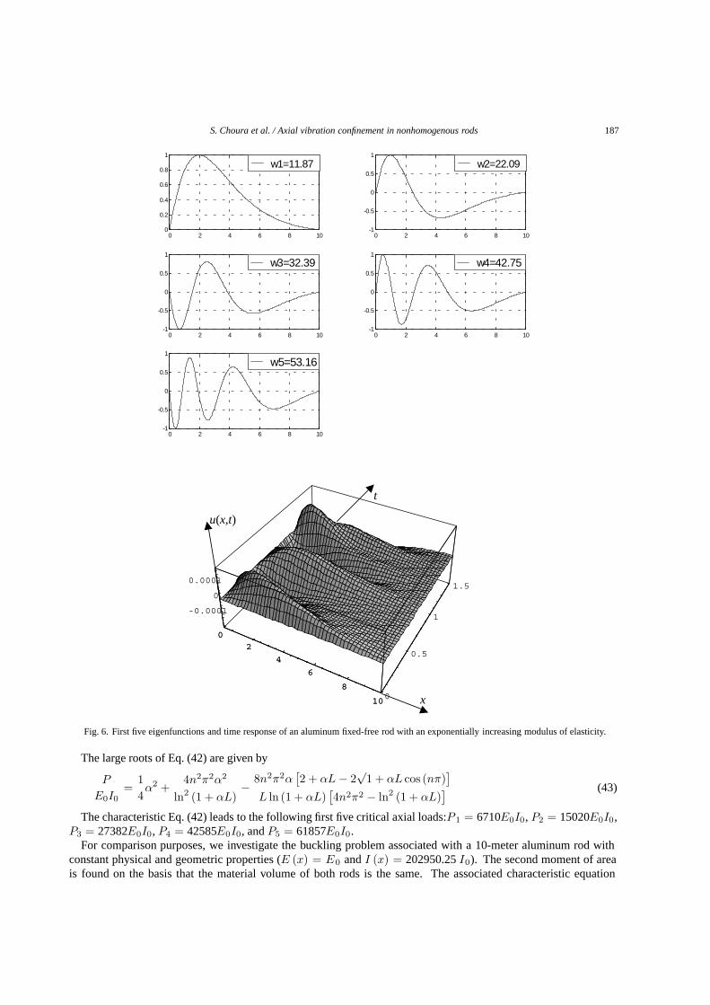
Fig. 6. First five eigenfunctions and time response of an aluminum fixed-free rod with an exponentially increasing modulus of elasticity.
The large roots of Eq. (42) are given by
P
E0I0=
14α2 +
4n2π2α2
ln2 (1 + αL)− 8n2π2α
[2 + αL − 2
√1 + αL cos (nπ)
]L ln (1 + αL)
[4n2π2 − ln2 (1 + αL)
] (43)
The characteristic Eq. (42) leads to the following first five critical axial loads:P 1 = 6710E0I0, P2 = 15020E0I0,P3 = 27382E0I0, P4 = 42585E0I0, and P5 = 61857E0I0.
For comparison purposes, we investigate the buckling problem associated with a 10-meter aluminum rod withconstant physical and geometric properties (E (x) = E0 and I (x) = 202950.25 I0). The second moment of areais found on the basis that the material volume of both rods is the same. The associated characteristic equation
188 S. Choura et al. / Axial vibration confinement in nonhomogenous rods
leads to the following first five critical axial loads: P1 = 80122E0I0, P2 = 163909E0I0, P3 = 320486E0I0,P4 = 484479E0I0, and P5 = 965230E0I0. Comparison of the two sets of critical axial loads shows that the relativedifferences are reduced remarkably in this case. The buckling problems in Sections 4 and 5 reveal that the spatialvariation of the cross-section area plays a major role in controlling the relative differences in the critical bucklingloads.
6. Exponentially varying modulus of elasticity
In this case, A (x) = A0, ρ (x) = ρ0, E (x) = E0eαx with α = 1L lnEL/E0 and EL > E0; that is, the
rigidity increases exponentially with respect to x making the rod stiffer in the vicinity of the right end. In practice,this could be the case of an FGM with constituent materials having the same density but different moduli of elasticity.Thus, Eq. (3) reduces to
d
dx
[eαx dU
dx
]+ ω2 ρ0
E0U = 0 (44)
For a fixed-fixed rod, the eigenfunctions are given by
Ui (x) = Cie−12 αx
⎡⎣J1
(κie−
12 αx)
J1 (κi)−
Y1
(κie−
12 αx)
Y1 (κi)
⎤⎦ i = 1, 2, . . . (45)
where κ2i = 4ρ0ω2
i
α2E0. The corresponding characteristic equation is
J1
(κie−
12 αL)
Y1 (κi) − J1 (κi)Y1
(κie−
12 αL)
= 0 (46)
For a 10-meter aluminum rod (E0 = 1.5 106 N / m2, EL = 1.5 108 N / m2, ρ0 = 8760 kg, L = 10 m,and A0 = 10−4 m2), Fig. 6 shows the first five eigenfunctions and the time response for an initial time velocitydistribution. This simulation confirms the confinement of vibrations in the neighborhood of the left end (x = 0).
As in previous cases, the associated buckling problem is defined as
d2
dx2
[eαx d2w
dx2
]+
P
E0I0
d2w
dx2= 0 w (0) = w (L) =
dw
dx(0) =
dw
dx(L) = 0 (47)
It can be verified that the solution associated with the above boundary-value problem can be expressed as
w (x) = C1 + C2x + C3J0
(λe−
12 αx)
+ C4Y0
(λe−
12 αx)
(48)
where λ2 = 4Pα2E0I0
. Applying the boundary conditions and letting L = 10 m, we obtain from the characteristicequation the following first five critical axial buckling loads: P1 = 2.68E0I0, P2 = 5.30E0I0, P3 = 10.47E0I0,P4 = 15.65E0I0, and P5 = 23.40E0I0.
For comparison purposes, we investigate the buckling problem associated with a 10-meter aluminum rod withconstant physical and geometric properties (E (x) = E0 and I (x) = I0). The second moment of area is keptthe same since the material volume of both rods is kept the same. The first five critical axial loads are found tobe P1 = 0.81E0I0, P2 = 2.39E0I0, P3 = 4.76E0I0, P4 = 7.91E0I0, and P5 = 11.86E0I0. In this case, thefirst critical axial load is enhanced, and therefore, a proper spatial variation of the modulus of elasticity producessimultaneous improvement in the vibration confinement and resistance to buckling.
We note that the homogeneous rod uses the minimum value of the spatially varying modulus of elasticityE (x) = E0 eαx. In case the average value 1
2 (E0 + EL) = 50.05 E0 is employed, then the critical bucklingloads become P1 = 40.54E0I0, P2 = 119.62E0I0, P3 = 238.24E0I0, P4 = 395.90E0I0, and P5 = 593.59E0I0.In this case, the critical loads associated with the spatially varying rod are lower than those of a homogeneous rod.
S. Choura et al. / Axial vibration confinement in nonhomogenous rods 189
7. Exponentially varying density
In this case, A (x) = A0, E (x) = E0, ρ (x) = ρ0 eβ x with β = 1L lnρL
ρ0and ρL > ρ0; that is, the density
increases exponentially with respect to x making the rod more dense in the vicinity of the right end. In practice, thiscould be the case of an FGM with constituent materials having the same modulus of elasticity but different densities.Thus, Eq. (3) reduces to
d2U
dx2+
ρ0ω2
E0eβxU = 0 (49)
For a fixed-fixed rod with, the eigenfunctions satisfying Eq. (49) are given by
Ui (x) = Ci
⎡⎣J0
(κie
12 βx)
J0 (κi)−
Y0
(κie
12 βx)
Y0 (κi)
⎤⎦ i = 1, 2, 3, . . . (50)
where κ2i = 4ρ0ω2
i
β2E0. The corresponding characteristic equation is
J0
(κie
12 βL)
Y0 (κi) − J0 (κi) Y0
(κie
12 βL)
= 0 (51)
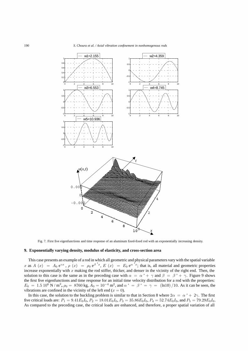
Figure 7 shows the first five eigenfunctions and the time response for an initial time velocity distribution for a rodwith the properties: E0 = 1.5 106 N / m2, ρ0 = 8760 kg, ρL = 87600 kg, L = 10 m, and A0 = 10−4 m2. Thisfigure clearly shows that the vibrations are confined towards the left end (x = 0).
8. Exponentially varying density and modulus of elasticity
In this case, A (x) = A0 , ρ (x) = ρ0eβx and E (x) = E0eαx ; that is, all physical properties increaseexponentially with respect to x making the rod stiffer and denser in the vicinity of the right end. In practice, thiscould be the case of an FGM with constituent materials having different densities and different moduli of elasticity.Thus, Eq. (3) reduces to
d
dx
[eαx dU
dx
]+
ρ0ω2
E0eβxU = 0 (52)
For a fixed-fixed rod, the eigenfunctions satisfying Eq. (52) are given by
Ui (x) = Cie−12 αx
⎡⎣Jν
(κie−
12 (α−β)x
)Jν (κi)
−Yν
(κie−
12 (α−β)x
)Jν (κi)
⎤⎦ i = 1, 2, 3, . . . (53)
where ν = αα − β , κ2
i = 4ρ0ω2i
(α − β)2E0, and α �= β. The corresponding characteristic equation is
Jν
(κie
− 12 (α−β)L
)Yν (κi) − Jν (κi)Yν
(κie
− 12 (α−β)L
)= 0 (54)
When α = β, the eigenfunctions that satisfy the left boundary condition can be expressed as
Ui (x) = Ci e−12 αxsin
[√ρ0ω2
i /E0 − α2x
]i = 1, 2, 3, . . . (55)
Therefore, the natural frequencies are given by
ωi =
√E0
ρ0
(n2π2
L2+ α2
)i = 1, 2, 3, . . . (56)
Figure 8 shows the first five eigenfunctions and time response for an initial time velocity distribution for a rodwith the properties: E0 = 1.5 × 10⁶ N / m2, ρ0 = 8760 kg, and A0 = 10−4 m2, α = β = ln (10) /10. As itcan be seen, the vibrations are confined in the vicinity of the left end (x = 0). The associated buckling problem isdefined by Eq. (47) whose solution is given by Eq. (48).
190 S. Choura et al. / Axial vibration confinement in nonhomogenous rods
0 2 4 6 8 100
0.2
0.4
0.6
0.8
1w1=2.155
0 2 4 6 8 10-1
-0.5
0
0.5
1w2=4.359
0 2 4 6 8 10-1
-0.5
0
0.5
1w3=6.553
0 2 4 6 8 10-1
-0.5
0
0.5
1w4=8.745
0 2 4 6 8 10-1
-0.5
0
0.5
1w5=10.936
0 2
4 6
8 10 0
2
4 -0.002
0
0.002
0 2
4 6
8 10 x
u(x,t)
t
Fig. 7. First five eigenfunctions and time response of an aluminum fixed-fixed rod with an exponentially increasing density.
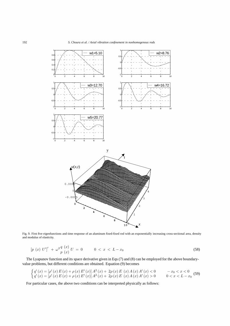
9. Exponentially varying density, modulus of elasticity, and cross-section area
This case presents an example of a rod in which all geometric and physical parameters vary with the spatial variablex as A (x) = A0 eγx , ρ (x) = ρ0 eβ ’x, E (x) = E0 eα ’x; that is, all material and geometric propertiesincrease exponentially with x making the rod stiffer, thicker, and denser in the vicinity of the right end. Then, thesolution to this case is the same as in the preceding case with α = α ’ + γ and β = β ’ + γ. Figure 9 showsthe first five eigenfunctions and time response for an initial time velocity distribution for a rod with the properties:E0 = 1.5 106 N / m2, ρ0 = 8760 kg, A0 = 10−4 m2, and α ’ = β ’ = γ = (ln10) /10. As it can be seen, thevibrations are confined in the vicinity of the left end (x = 0).
In this case, the solution to the buckling problem is similar to that in Section 8 where 2α = α ’ + 2γ. The firstfive critical loads are: P1 = 9.41E0I0, P2 = 18.01E0I0, P3 = 35.86E0I0, P4 = 52.74E0I0, and P5 = 79.29E0I0.As compared to the preceding case, the critical loads are enhanced, and therefore, a proper spatial variation of all
S. Choura et al. / Axial vibration confinement in nonhomogenous rods 191
0 2 4 6 8 100
0.2
0.4
0.6
0.8
1
w1=4.38
0 2 4 6 8 10-1
-0.5
0
0.5
1
w2=8.36
0 2 4 6 8 10-1
-0.5
0
0.5
1
w3=12.42
0 2 4 6 8 10-1
-0.5
0
0.5
1
w4=16.51
0 2 4 6 8 10-1
-0.5
0
0.5
1
w5=20.61
0 2
4 6
8 10 0
1
2
3
4
-0.0005 -0.00025
0 0.00025 0.0002
0
2 4
6 8
10 x
u(x,t)
t y
Fig. 8. First five eigenfunctions and time response of an aluminum fixed-fixed rod with an exponentially increasing density and modulus ofelasticity.
parameters is capable of producing a simultaneous improvement of vibration confinement and rod resistance tobuckling.
10. Confinement at an interior region
If one wishes to confine the vibrations about an arbitrary point x 0 instead of the origin, then the feedback forcemust be altered as follows: first, we shift the origin to x0, the point about which the vibrations to be confined. Now,the boundary-value problems associated with the rod are:
[p (x) U ′]′ + ω2 q (x)p (x)
U = 0 − x0 < x < 0 (57)
192 S. Choura et al. / Axial vibration confinement in nonhomogenous rods
0 2 4 6 8 100
0.2
0.4
0.6
0.8
1
w1=5.10
0 2 4 6 8 10-1
-0.5
0
0.5
1
w2=8.76
0 2 4 6 8 10-1
-0.5
0
0.5
1
w3=12.70
0 2 4 6 8 10-1
-0.5
0
0.5
1
w4=16.72
0 2 4 6 8 10-1
-0.5
0
0.5
1
w5=20.77
0 2
4 6
8 10 0
1
2
3
4
-0.0005
0
0.0005
0 2
4 6
8 10 x
u(x,t)
t
y
Fig. 9. First five eigenfunctions and time response of an aluminum fixed-fixed rod with an exponentially increasing cross-sectional area, densityand modulus of elasticity.
[p (x) U ′]′ + ω2 q (x)p (x)
U = 0 0 < x < L − x0 (58)
The Lyapunov function and its space derivative given in Eqs (7) and (8) can be employed for the above boundary-value problems, but different conditions are obtained. Equation (9) becomes{
q′ (x) = [ρ′ (x) E (x) + ρ (x) E′ (x)] A2 (x) + 2ρ (x) E (x)A (x)A′ (x) < 0 − x0 < x < 0q′ (x) = [ρ′ (x) E (x) + ρ (x) E′ (x)] A2 (x) + 2ρ (x) E (x)A (x)A′ (x) > 0 0 < x < L − x0
(59)
For particular cases, the above two conditions can be interpreted physically as follows:
S. Choura et al. / Axial vibration confinement in nonhomogenous rods 193
Fig. 10. Shape of a rod producing vibration confinement at the middle point.
1. keep both of the modulus of elasticity and the density constant across the rod and vary the cross-sectionarea provided that its spatial derivative with respect to x is negative for − x0 < x < 0 and positive for0 < x < L − x0. This implies that the rod shape decreases up to x0 and then increases up to the right endof the rod,
2. keep both of the modulus of elasticity and the cross-section area constant across the rod and vary the densityprovided that its spatial derivative with respect to x is negative for − x0 < x < 0 and positive for0 < x < L − x0. This implies that the rod density decreases up to x0 and then increases up to the rightend of the rod,
3. keep both of the density and cross-section area constant across the rod and vary the modulus of elasticityprovided that its spatial derivative with respect to x is negative for − x0 < x < 0 and positive for0 < x < L − x0. This implies that the rod stiffness decreases up to x0 and then increases up to the rightend of the rod.
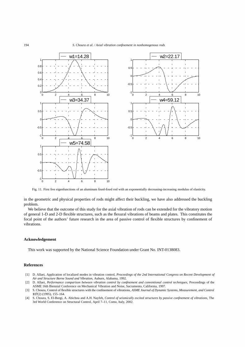
Figure 10 shows a particular shape of the rod that produces vibration confinement at the middle of the rod (bothmodulus of elasticity and density are constant and the cross-section area is variable). As another illustration, let usconsider a beam whose modulus of elasticity varies according to the following distribution function:
E (x) =
⎧⎨⎩E0e
(ln
Ex0E0
)x
x0 0 < x < x0
Ex0e
(ln
ELEx0
)(x−x0)L−x0 x0 < x < L
(60)
where E0 > Ex0 and EL > Ex0 . This implies that the modulus of elasticity is an exponentially decaying functionof x for 0 < x < x0 and is an exponentially increasing function of x in the interval x 0 < x < L. Fora rod of constant density (ρ0 = 8760 Kg / m3), constant cross-section area (A0 = 10−4 m2), L = 10 meter,x0 = 5 meter, E0 = EL = 1.5 × 10⁸N / m2, and Ex0 = 1.5 × 10⁶N / m2, Fig. 11 shows the first five modeshapes associated with the distribution given by Eq. (60). Applying the boundary conditions associated with thebuckling problem, the characteristic equation leads to the following first five critical axial loads: P 1 = 0.54E0I0,P2 = 3.91E0I0, P3 = 8.58E0I0, P4 = 14.31E0I0, and P5 = 16.27E0I0. Compared to the case of constantmaterial and geometric properties, we conclude that the first critical buckling load is reduced by 33% while thesecond, third, fourth, and fifth critical loads are increased by 64%, 80%, 81% and 37%, respectively.
11. Conclusions
This paper is concerned with the design of spatially-dependent functions characterizing structure material andgeometric properties for the confinement of rod axial vibrations. The aim is to develop a set of rod parametersthat lead to reallocating its vibratory energy so that vibrations are reduced in the sensitive parts and increased inthe remaining parts. The selection of such properties is accomplished by constructing positive Lyapunov functionswhose derivative with respect to the space variable is negative. In case both of the density and modulus of elasticityare kept constant while the cross-section area is varied, vibration confinement requires that the eigenfunctions beexponentially decaying functions of space, where the notion of spatial domain stability is introduced as a concept dualto that of time-domain stability. Thus, varying the shape of the rod alone is sufficient to confine the vibratory motion.We have also shown that vibration confinement can be produced if one (or both) of the rod density and stiffness isvaried with respect to the space variable while the cross-section area is kept constant. Several cases, supporting thedeveloped conditions imposed on the spatially-dependent functions, are discussed and simulated. Because variations
194 S. Choura et al. / Axial vibration confinement in nonhomogenous rods
0 2 4 6 8 100
0.2
0.4
0.6
0.8
1w1=14.28
0 2 4 6 8 10-1
-0.5
0
0.5
1w2=22.17
0 2 4 6 8 10-1
-0.5
0
0.5
1w3=34.37
0 2 4 6 8 10-1
-0.5
0
0.5
1w4=59.12
0 2 4 6 8 10-1
-0.5
0
0.5
1w5=74.58
Fig. 11. First five eigenfunctions of an aluminum fixed-fixed rod with an exponentially decreasing-increasing modulus of elasticity.
in the geometric and physical properties of rods might affect their buckling, we have also addressed the bucklingproblem.
We believe that the outcome of this study for the axial vibration of rods can be extended for the vibratory motionof general 1-D and 2-D flexible structures, such as the flexural vibrations of beams and plates. This constitutes thefocal point of the authors’ future research in the area of passive control of flexible structures by confinement ofvibrations.
Acknowledgement
This work was supported by the National Science Foundation under Grant No. INT-0138083.
References
[1] D. Allaei, Application of localized modes in vibration control, Proceedings of the 2nd International Congress on Recent Development ofAir and Structure Borne Sound and Vibration, Auburn, Alabama, 1992.
[2] D. Allaei, Performance comparison between vibration control by confinement and conventional control techniques, Proceedings of theASME 16th Biennial Conference on Mechanical Vibration and Noise, Sacramento, California, 1997.
[3] S. Choura, Control of flexible structures with the confinement of vibrations, ASME Journal of Dynamic Systems, Measurement, and Control117(2) (1995), 155–164.
[4] S. Choura, S. El-Borgi, A. Abichou and A.H. Nayfeh, Control of seismically excited structures by passive confinement of vibrations, The3rd World Conference on Structural Control, April 7–11, Como, Italy, 2002.
S. Choura et al. / Axial vibration confinement in nonhomogenous rods 195
[5] S. Choura and A.S. Yigit, Vibration confinement in flexible structures by distributed feedback, Journal of Computers and Structures 54(3)(1995), 531–540.
[6] S. Choura and A.S. Yigit, Confinement and suppression of structural vibrations, ASME Journal of Vibration and Acoustics 123 (October,2001), 496–501.
[7] M.T.C. Chu, Inverse eigenvalue problems, SIAM Review 40 (1998), 1–39.[8] F. Erdogan, Fracture Mechanics of Functionally Graded Materials, Composites Engineering 5 (1995), 753–770.[9] M.M. Fahmy and J. O’Reilly, On eigenstructure assignment in linear multivariable system, IEEE Transactions on Automatic Control
AC-27(3) (1982), 690–693.[10] J.N. Juang, K.B. Lim and J.L. Junkins, Robust eigensystem assignment for flexible structures, Journal of Guidance, Control, and Dynamic
12 (1989), 311–317.[11] J. Kautsy, N.K. Nichols and O. Van Dooren, Robust pole assignment in linear state Feedback, International Journal of Control 41(5)
(1985), 1229–1245.[12] T. Kobori and S. Kamagata, Dynamic intelligent buildings-active seismic response control, Intelligent Structures-2, 1992, pp. 279–282,
Y.K. Wen, ed., Elsevier Applied Science, New York.[13] B.S. Liebst and W.L. Garrard, Application of eigenspace techniques to design of aircraft control systems, Proceedings of the 1985 American
Control Conference, June 1985, pp. 475–480, Boston, Massachusetts.[14] P.G. Maghami and S. Gupta, On the eigensystem assignment with dissipativity constraints, Proceedings of the 1993 American Control
Conference, June 1993, pp. 1271–1275, San Francisco, California.[15] P.G. Maghami, J. Juang and K.B. Lim, Eigensystem assignment with output feedback, Journal of Guidance, Control, and Dynamics 15
(1993), 531–536.[16] Y.M. Ram, Pole assignment for the vibrating rod, Quarterly Journal of Mechanics and Applied Mathematics 51(3) (1998), 477–492.[17] Y.M. Ram and S. Elhay, An inverse eigenvalue problem for the symmetric tridiagonal quadratic pencil with application of damped
oscillatory systems, SIAM Journal on Applied Mathematics 56(1) (1996), 232–244.[18] Y.M. Ram and S. Elhay, Constructing the shape of a rod from eigenvalues, Communications in Numerical Methods in Engineering 14(7)
(1998), 597–608.[19] J. Shaw and S. Jayasuriya, Arbitrary assignment of eigenvectors with state feedback, ASME Journal of Dynamic Systems, Measurement
and Control 114 (1992), 721–723.[20] D.D. Sivan and Y.M. Ram, Physical modifications to vibratory systems with assigned eigendata, ASME Journal of Applied Mechanics
66(2) (1999), 427–432.[21] K.M. Sobel, E.Y. Shapiro and A.N. Andry Jr., Eigenstructure assignment, International Journal of Control 59 (1994), 13–37.[22] B.K. Song and S. Jayasuriya, Active vibration control using eigenvector assignment for mode localization, Proceedings of the 1993
American Control Conference, June 1993, 1020–1024, San Francisco, California.[23] R.F. Wilson, J.R. Cloutier and R.K. Yedaveli, Control design for robust eigenstructure assignment in linear uncertain systems, IEEE Control
Systems Magazine 12(5) (1992), 29–34.[24] A.S. Yigit and S. Choura, Vibration confinement in flexible structures via alteration of mode shapes using feedback, Journal of Sound and