Axial vs. equatorial dipolar dynamo models with implications for planetary magnetic fields

Axial vs. equatorial dipolar dynamo models withimplications for planetary magnetic ¢elds

Julien Aubert �, Johannes WichtMax-Planck-Institute for Aeronomy, Max-Planck-Strasse 2, 37191 Katlenburg-Lindau, Germany

Received 3 July 2003; received in revised form 27 January 2004; accepted 29 January 2004

Abstract

We present several numerical simulations of a self-consistent dynamo model in a rotating spherical shell. Thesolutions have two different field configurations. Besides magnetic fields dominated by the axial dipole component, wealso find configurations where a dipole in the equatorial plane is the dominating component. Both types are stable ina parameter regime of intermediate shell thickness and Rayleigh numbers close to onset of convection. Axial dipolesolutions are subcritical in all the simulations explored while the equatorial dipole cases are supercritical at lowRayleigh numbers but become metastable at higher Rayleigh numbers. The magnetic field strength saturates at amuch lower amplitude for the equatorial dipole dynamos, and the Elsasser number is significantly smaller than in theaxial configuration. The reason is that the mainly horizontal field in the equatorial dipole solution is incompatiblewith the motion of convective cyclones and anticyclones. The axial dipole field, on the other hand, is predominantlyaligned with the axis of anticyclones, only cyclones are disrupted by horizontal field lines passing through. Thisconfiguration can therefore accomodate stronger convective flows and, consequently, is the only one remaining stableat higher Rayleigh numbers. These arguments should pertain in all planetary dynamos that are governed by strongrotational constraints. They offer an explanation why the Elsasser numbers inferred for Uranus and Neptune aremuch lower than the Elsasser numbers of Jupiter, Saturn, and Earth./ 2004 Elsevier B.V. All rights reserved.

Keywords: numerical dynamo simulation; axial dipole; equatorial dipole; Uranus; Neptune; magnetic ¢eld

1. Introduction

Before the spacecraft Voyager II visited Uranusand Neptune it was consensus that planetarymagnetic ¢elds are dominated by a dipole alignedwith the planetary rotation axis. The magnetic

¢elds of the Earth, Saturn, Jupiter, and probablyalso Mercury, fall into this category. But the mag-netic ¢elds of Uranus and Neptune are di¡erent.Their dipole axes are tilted at 50‡ and 47‡, respec-tively, to the planetary spin axis. Global ¢eldmodels also show that both planetary magnetic¢elds have signi¢cant quadrupole and octupolecontributions [1], much larger than, for example,in the geomagnetic ¢eld.

Kinematic dynamo calculations have demon-strated that axial dipole con¢gurations are more

0012-821X / 04 / $ ^ see front matter / 2004 Elsevier B.V. All rights reserved.doi:10.1016/S0012-821X(04)00102-5

* Corresponding author. Tel. : +49-5556-9790;Fax: +49-5556-979-240.E-mail address: [email protected] (J. Aubert).

EPSL 7038 25-3-04 Cyaan Magenta Geel Zwart

Earth and Planetary Science Letters 221 (2004) 409^419

R

Available online at www.sciencedirect.com

www.elsevier.com/locate/epsl

mailto:[email protected]

http://www.elsevier.com/locate/epsl

frequent. Some of the tested £ows neverthelessfavor equatorial dipole solutions [1,2]. Likewise,the magnetic ¢eld measured in the Karlsruhe dy-namo experiment [3] is equivalent to a dipole ly-ing in the equatorial plane. Most of the self-con-sistent dynamo simulations, on the other hand,are geared to model the geodynamo and featuresolutions dominated by an axial dipole [4^6]. Theequatorial dipole contribution may only dominatein a transient state during a reversal. An excep-tion is the self-consistent simulation by Ishiharaand Kida [7]. They ¢nd a persisting equatorialdipole solution at a critical Rayleigh number closeto onset of convection. However, when they dou-ble the Rayleigh number the solution switches toan axial dipole dominated con¢guration.

Here, we present a region of the parameterspace where dynamos of both con¢gurations cancoexist. We highlight important di¡erences in therespective dynamo mechanisms and discuss ourresults within the scope of planetary applications.For simplicity we will refer to axial and equatorialdipole solutions for magnetic ¢elds which aredominated by the respective dipole component.All solutions presented here also contain higher¢eld harmonics in addition to the dipole. Axialand equatorial dipoles are representatives of twodi¡erent symmetry classes. The axial dipole ¢eldis antisymmetric with respect to the equator whilethe equatorial dipole ¢eld is symmetric. Confus-ingly, these two classes are sometimes referred toas dipole and quadrupole dynamos, because axi-symmetric ¢elds are thought to be the dominantcontributions in both symmetry classes. Grote etal. [8] have explored the parameter space for theexistence of dipolar and quadrupolar dynamos.Contrary to the results presented here, their solu-tions are always dominated by axisymmetric com-ponents.

2. Numerical model

We study the dynamo action in an electricallyconducting, thermally convecting Boussinesq £u-id. The £uid is contained in a spherical shell thatrotates about the z-axis with rotation rate 6. Weformulate a dimensionless model and use the shell

thickness, i.e. the di¡erence between inner andouter shell radii ri and re, as a length scale. Themagnetic di¡usion time D2/R serves as the timescale, and the Elsasser number (bWR6)1=2 scalesmagnetic induction B. Here, R is the magneticdi¡usivity of the £uid, b is the £uid density, andW the magnetic permeability.

The boundaries are isothermal and the di¡er-ence between inner and outer boundary temper-ature, Ti and To, respectively, is used as the tem-perature scale. The dimensionless equation systemincludes the Navier^Stokes equation, the dynamoequation, the heat equation, the simpli¢ed con-tinuity equation, and the condition that magneticinduction is divergence free:

EqPr

D uD t

þ uW9u� �

þ 2ezUu ¼

392þ Ra q PrrreerT þ ð9UBÞUBþ E92u ð1Þ

dBdt

¼ 9UðuUBÞ þ 92B ð2ÞDTD t

þ uW9T ¼ q92T ð3Þ

9Wu ¼ 0: ð4Þ

9WB ¼ 0 ð5ÞThe non-dimensional control parameters are

the Rayleigh number Ra, the Ekman number E,the Prandtl number Pr, the Roberts number q,and the radius ratio Q :

Ra ¼ KgovTDX6

ð6Þ

E ¼ X

6D2 ð7Þ

Pr ¼ X

Uð8Þ

q ¼ U

R

ð9Þ

Q ¼ rire

ð10Þ

The additional material parameters used here arethe kinematic viscosity X, the thermal di¡usivity U,the thermal expansion coe⁄cient K, and gravity goat outer radius ro.

Rigid conditions are used for the velocity atboth boundaries. The inner core is electrically


J. Aubert, J. Wicht / Earth and Planetary Science Letters 221 (2004) 409^419410

conducting and rotates under the in£uence ofLorentz and viscous torques. An inner core dyna-mo equation and the inner core angular momen-tum budget are solved simultaneously with thesystem of Eqs. 1^5. The outer boundary is treatedas an electrical insulator. Pseudospectral methodsare employed with spherical harmonics up to de-gree 53 for the horizontal representation and Che-byshev polynomials up to degree 30 in radius. Theequation system is time-stepped with a mixed im-plicit/explicit algorithm. For more details on thenumerical model we refer to [6,9].

3. Results

3.1. Stability of axial and equatorial dynamos

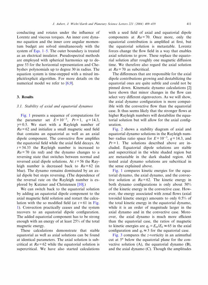
Fig. 1 presents a sequence of computations forthe parameter set E=1033, Pr=1, q=14.3,Q=0.5. We start with a Rayleigh number ofRa=62 and initialize a small magnetic seed ¢eldthat contains an equatorial as well as an axialdipole component. The convective £ow ampli¢esthe equatorial ¢eld while the axial ¢eld decays. Att=54.33 the Rayleigh number is increased toRa=70 (in red) and the dynamo changes to areversing state that switches between normal andreversed axial dipole solutions. At t=56 the Ray-leigh number is decreased back to Ra=62 (inblue). The dynamo remains dominated by an ax-ial dipole but stops reversing. (The dependence ofthe reversal rate on the Rayleigh number is ex-plored by Kutzner and Christensen [10].)

We can switch back to the equatorial solutionby adding an equatorial dipole component to theaxial magnetic ¢eld solution and restart the calcu-lation with the so modi¢ed ¢eld (at t=61 in Fig.1). Convection practically ceases and the systemrecovers to an equatorial dipole con¢guration.The added equatorial component has to be strongenough with an energy of at least 25% of the totalmagnetic energy.

These calculations demonstrate that stableequatorial as well as axial solutions can be foundat identical parameters. The axial solution is sub-critical at Ra=62 while the equatorial solution issupercritical. We have also started calculations

with a seed ¢eld of axial and equatorial dipolecomponents at Ra=70. Once more, only theequatorial contribution is ampli¢ed at ¢rst, butthe equatorial solution is metastable. Lorentzforces change the £ow ¢eld in a way that enablesaxial solutions to grow. These replace the equato-rial solution after roughly one magnetic di¡usiontime. We therefore also regard the axial solutionat Ra=70 as subcritical.

The di¡erences that are responsible for the axialdipole contributions growing and destabilizing theequatorial ones are quite subtle and could not bepinned down. Kinematic dynamo calculations [2]have shown that minor changes in the £ow canselect very di¡erent eigenvectors. As we will show,the axial dynamo con¢guration is more compat-ible with the convective £ow than the equatorialcase. It thus seems likely that the stronger £ows athigher Rayleigh numbers will destabilize the equa-torial solution but will allow for the axial con¢g-uration.

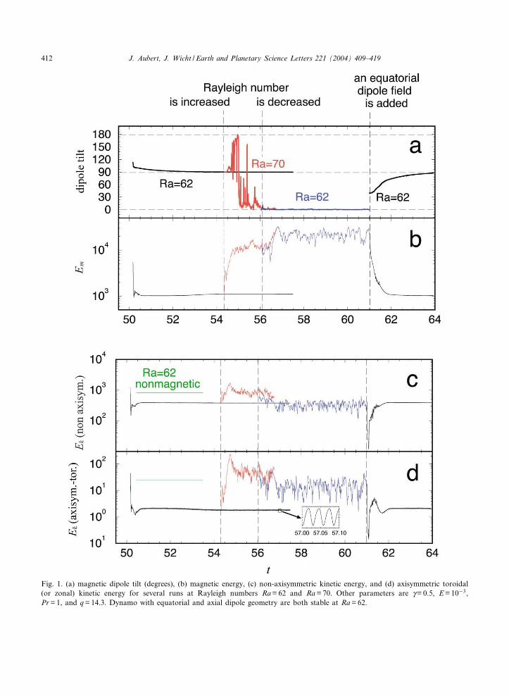
Fig. 2 shows a stability diagram of axial andequatorial dynamo solutions in the Rayleigh num-ber^radius ratio space for E=1033, q=14.3, andPr=1. The solutions described above are in-cluded. Equatorial dipole solutions are stableand supercritical in the white shaded region butare metastable in the dark shaded region. Alltested axial dynamo solutions are subcritical inthe sense explained above.

Fig. 1 compares kinetic energies for the equa-torial dynamo, the axial dynamo, and the convec-tive solution at Ra=62. The kinetic energy inboth dynamo con¢gurations is only about 50%of the kinetic energy in the convective case. How-ever, the energy associated with zonal £ows (axialtoroidal kinetic energy) amounts to only 0.5% ofthe total kinetic energy in the equatorial dynamo,while it is an order of magnitude larger in theaxial dynamo and in the convective case. More-over, the axial dynamo is much more e⁄cientthan the equatorial case, the ratios of magneticto kinetic energies are qe =Em/EkW65 in the axialcon¢guration and qeW3 for the equatorial case.

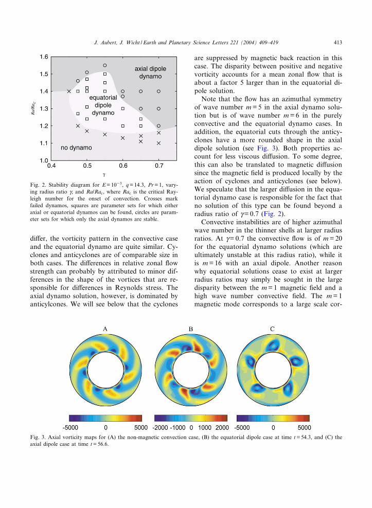
Fig. 3 compares the z-vorticity in an azimuthalcut at 5‡ below the equatorial plane for the con-vective solution (A), the equatorial dynamo (B),and the axial dynamo (C). Though the amplitudes


J. Aubert, J. Wicht / Earth and Planetary Science Letters 221 (2004) 409^419 411

Fig. 1. (a) magnetic dipole tilt (degrees), (b) magnetic energy, (c) non-axisymmetric kinetic energy, and (d) axisymmetric toroidal(or zonal) kinetic energy for several runs at Rayleigh numbers Ra=62 and Ra=70. Other parameters are Q=0.5, E=1033,Pr=1, and q=14.3. Dynamo with equatorial and axial dipole geometry are both stable at Ra=62.



di¡er, the vorticity pattern in the convective caseand the equatorial dynamo are quite similar. Cy-clones and anticyclones are of comparable size inboth cases. The di¡erences in relative zonal £owstrength can probably by attributed to minor dif-ferences in the shape of the vortices that are re-sponsible for di¡erences in Reynolds stress. Theaxial dynamo solution, however, is dominated byanticylcones. We will see below that the cyclones

are suppressed by magnetic back reaction in thiscase. The disparity between positive and negativevorticity accounts for a mean zonal £ow that isabout a factor 5 larger than in the equatorial di-pole solution.

Note that the £ow has an azimuthal symmetryof wave number m=5 in the axial dynamo solu-tion but is of wave number m=6 in the purelyconvective and the equatorial dynamo cases. Inaddition, the equatorial cuts through the anticy-clones have a more rounded shape in the axialdipole solution (see Fig. 3). Both properties ac-count for less viscous di¡usion. To some degree,this can also be translated to magnetic di¡usionsince the magnetic ¢eld is produced locally by theaction of cyclones and anticyclones (see below).We speculate that the larger di¡usion in the equa-torial dynamo case is responsible for the fact thatno solution of this type can be found beyond aradius ratio of Q=0.7 (Fig. 2).

Convective instabilities are of higher azimuthalwave number in the thinner shells at larger radiusratios. At Q=0.7 the convective £ow is of m=20for the equatorial dynamo solutions (which areultimately unstable at this radius ratio), while itis m=16 with an axial dipole. Another reasonwhy equatorial solutions cease to exist at largerradius ratios may simply be sought in the largedisparity between the m=1 magnetic ¢eld and ahigh wave number convective ¢eld. The m=1magnetic mode corresponds to a large scale cor-

Fig. 2. Stability diagram for E=1033, q=14.3, Pr=1, vary-ing radius ratio Q, and Ra/Rac, where Rac is the critical Ray-leigh number for the onset of convection. Crosses markfailed dynamos, squares are parameter sets for which eitheraxial or equatorial dynamos can be found, circles are param-eter sets for which only the axial dynamos are stable.

Fig. 3. Axial vorticity maps for (A) the non-magnetic convection case, (B) the equatorial dipole case at time t=54.3, and (C) theaxial dipole case at time t=56.6.





relation in azimuth, which is not very likely con-sidering the small scale £ow background thatfeeds the magnetic ¢eld.

3.2. Nature of the axial dipole dynamo

The axial dipole dynamo is similar in natureand mechanism to the K

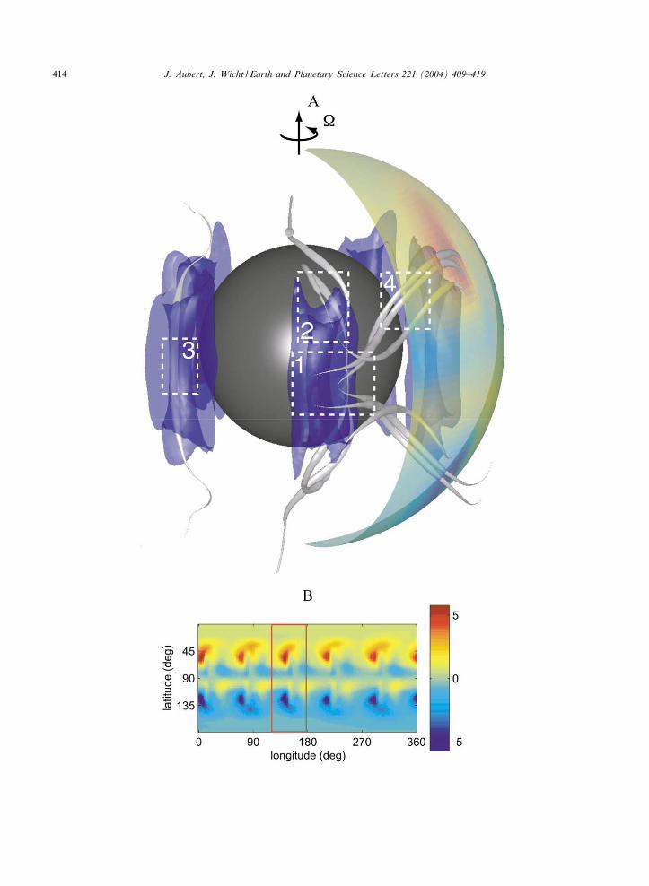
2 dynamos studied earlier[6]. We present a new visualization (Fig. 4) thathighlights di¡erences between the equatorial andaxial dipole mechanisms and refer to [6] for amore detailed analysis. Fig. 4A shows anticy-clones, selected magnetic ¢eld lines, and the innercore. Also shown is a section of the outer bound-ary with color-coded radial magnetic ¢eld, out-ward (inward) directed ¢eld in plotted in red(blue). Anticyclones are represented by blue iso-surfaces of negative axial vorticity, cyclones havea much lower amplitude and are not shown here.

The rendered magnetic ¢eld lines illustrate the¢eld^vortex interaction. Their thickness has beenweighted with the magnetic pressure B2. This rep-resentation has several advantages. First, it allowsto judge which lines are energetically important.Second, it gives an idea of the Lorentz forces act-ing perpendicular to the line. The Lorentz forcecan be interpreted as the sum of a magnetic ten-sion and a magnetic pressure gradient:

ð9UBÞUB ¼ ðBW9ÞB39B2

2

� �� : ð11Þ

We switch to a local curvilinear coordinate sys-tem that is spanned by the tangential unit vectores along the ¢eld line, the normal unit vector en inthe local ¢eld line plane, and the binormal vectoreb = esUen. Magnetic tension is then given by:

ðBW9ÞB ¼ B2

Rcen þ

D

D sB2

2

� �es: ð12Þ

Here, Rc is the local curvature radius and s isthe coordinate along es. Plugging this into theLorentz force expression Eq. 11 results in:

ð9UBÞUB ¼ B2

Rcen39H

B2

2

� �� : ð13Þ

with 9H =93esD/Ds. The Lorentz force is thusstrong where magnetic pressure and ¢eld line cur-vature are large. Moreover, magnetic pressurevariations between adjacent lines carry informa-tion on the Lorentz force.

Fig. 4 indicates that the magnetic pressure in-side the anticyclones (area 3) is larger than attheir perimeter (areas 1 and 2). The respectivemagnetic pressure gradient is mainly balancedby the Coriolis force. The strong poloidal ¢eldlines sitting in the center of the antivortices arealigned with the vortex axis (area 3). Responsiblefor the alignment is a secondary £ow directedaway from the equator towards the northernand southern end of the vortex columns. This£ow plays an important role in the poloidal ¢eldproduction [6]. Axially aligned ¢eld minimizes the£ow disruption due to Lorentz forces.

The picture is di¡erent for the cyclones, wherethe internal secondary £ow is directed equator-wards. It collects magnetic ¢eld near the outerboundary and stretches the ¢eld lines down thecolumnar axis (area 4). However, the ¢eld isalso expelled from the vortex resulting in strong¢eld lines that cross the vorticity structure (lowerpart of area 4). The associated Lorentz forcebrakes the vortex motion and is responsible forthe dominance of anticyclones in the system, asobserved in an earlier study [11]. Note that thisselection of anticyclones is the result of a mag-netic instability. Flow instabilities also tend tofavor anticyclones but only at considerably higherRayleigh numbers [12].

3.3. The equatorial dipole dynamo mechanism

Fig. 5 illustrates the ¢eld con¢guration in theequatorial dynamo solutions. The ¢eld is mainlysymmetric with respect to the equator but also

6

Fig. 4. The axial dipolar dynamo at t=56.6. (A) Axial vorticity isosurface (value 31400), and magnetic ¢eld lines. The line thick-ness is weighted by B2. (B) Radial component of the magnetic ¢eld at the outer boundary (red is outwards). The zone within thered rectangle is represented on image A.



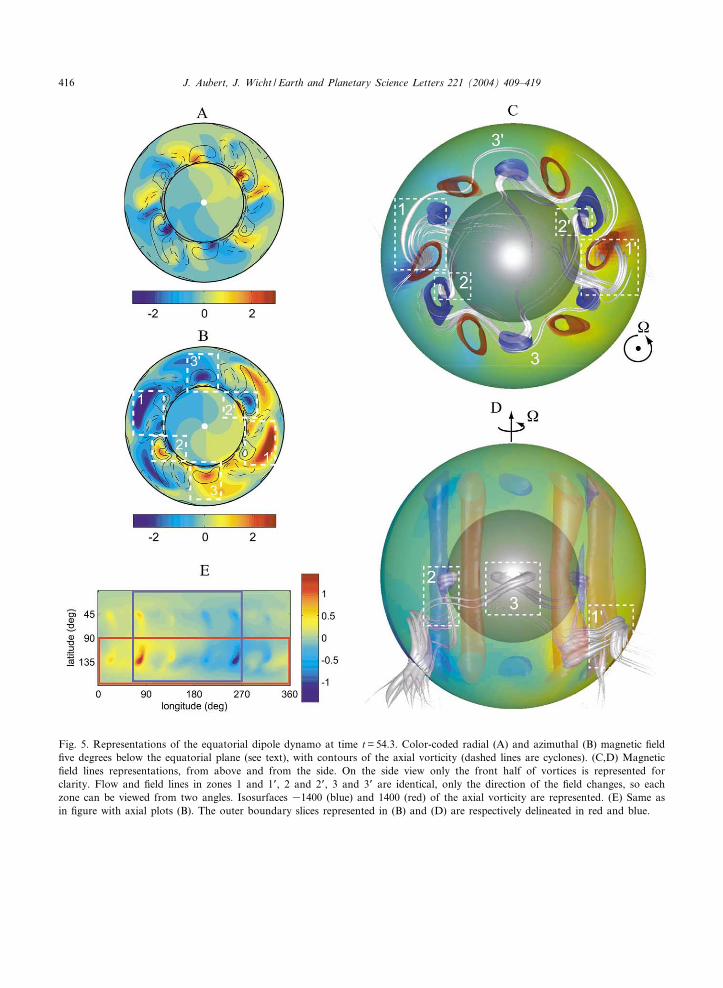
Fig. 5. Representations of the equatorial dipole dynamo at time t=54.3. Color-coded radial (A) and azimuthal (B) magnetic ¢eld¢ve degrees below the equatorial plane (see text), with contours of the axial vorticity (dashed lines are cyclones). (C,D) Magnetic¢eld lines representations, from above and from the side. On the side view only the front half of vortices is represented forclarity. Flow and ¢eld lines in zones 1 and 1P, 2 and 2P, 3 and 3P are identical, only the direction of the ¢eld changes, so eachzone can be viewed from two angles. Isosurfaces 31400 (blue) and 1400 (red) of the axial vorticity are represented. (E) Same asin ¢gure with axial plots (B). The outer boundary slices represented in (B) and (D) are respectively delineated in red and blue.



has a non-negligible antisymmetric component(see Fig. 5E). For simplicity we will neglect thelatter in the following exploration.

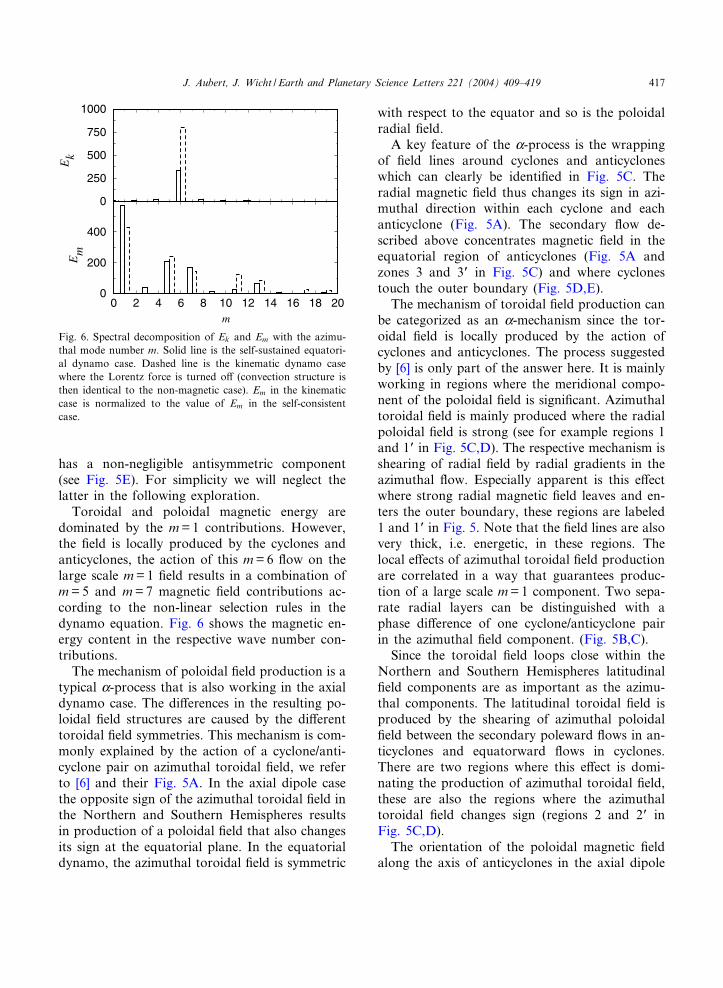
Toroidal and poloidal magnetic energy aredominated by the m=1 contributions. However,the ¢eld is locally produced by the cyclones andanticyclones, the action of this m=6 £ow on thelarge scale m=1 ¢eld results in a combination ofm=5 and m=7 magnetic ¢eld contributions ac-cording to the non-linear selection rules in thedynamo equation. Fig. 6 shows the magnetic en-ergy content in the respective wave number con-tributions.

The mechanism of poloidal ¢eld production is atypical K-process that is also working in the axialdynamo case. The di¡erences in the resulting po-loidal ¢eld structures are caused by the di¡erenttoroidal ¢eld symmetries. This mechanism is com-monly explained by the action of a cyclone/anti-cyclone pair on azimuthal toroidal ¢eld, we referto [6] and their Fig. 5A. In the axial dipole casethe opposite sign of the azimuthal toroidal ¢eld inthe Northern and Southern Hemispheres resultsin production of a poloidal ¢eld that also changesits sign at the equatorial plane. In the equatorialdynamo, the azimuthal toroidal ¢eld is symmetric

with respect to the equator and so is the poloidalradial ¢eld.

A key feature of the K-process is the wrappingof ¢eld lines around cyclones and anticycloneswhich can clearly be identi¢ed in Fig. 5C. Theradial magnetic ¢eld thus changes its sign in azi-muthal direction within each cyclone and eachanticyclone (Fig. 5A). The secondary £ow de-scribed above concentrates magnetic ¢eld in theequatorial region of anticyclones (Fig. 5A andzones 3 and 3P in Fig. 5C) and where cyclonestouch the outer boundary (Fig. 5D,E).

The mechanism of toroidal ¢eld production canbe categorized as an K-mechanism since the tor-oidal ¢eld is locally produced by the action ofcyclones and anticyclones. The process suggestedby [6] is only part of the answer here. It is mainlyworking in regions where the meridional compo-nent of the poloidal ¢eld is signi¢cant. Azimuthaltoroidal ¢eld is mainly produced where the radialpoloidal ¢eld is strong (see for example regions 1and 1P in Fig. 5C,D). The respective mechanism isshearing of radial ¢eld by radial gradients in theazimuthal £ow. Especially apparent is this e¡ectwhere strong radial magnetic ¢eld leaves and en-ters the outer boundary, these regions are labeled1 and 1P in Fig. 5. Note that the ¢eld lines are alsovery thick, i.e. energetic, in these regions. Thelocal e¡ects of azimuthal toroidal ¢eld productionare correlated in a way that guarantees produc-tion of a large scale m=1 component. Two sepa-rate radial layers can be distinguished with aphase di¡erence of one cyclone/anticyclone pairin the azimuthal ¢eld component. (Fig. 5B,C).

Since the toroidal ¢eld loops close within theNorthern and Southern Hemispheres latitudinal¢eld components are as important as the azimu-thal components. The latitudinal toroidal ¢eld isproduced by the shearing of azimuthal poloidal¢eld between the secondary poleward £ows in an-ticyclones and equatorward £ows in cyclones.There are two regions where this e¡ect is domi-nating the production of azimuthal toroidal ¢eld,these are also the regions where the azimuthaltoroidal ¢eld changes sign (regions 2 and 2P inFig. 5C,D).

The orientation of the poloidal magnetic ¢eldalong the axis of anticyclones in the axial dipole

Fig. 6. Spectral decomposition of Ek and Em with the azimu-thal mode number m. Solid line is the self-sustained equatori-al dynamo case. Dashed line is the kinematic dynamo casewhere the Lorentz force is turned o¡ (convection structure isthen identical to the non-magnetic case). Em in the kinematiccase is normalized to the value of Em in the self-consistentcase.



case plays no important role in the equatorial di-pole solutions. Here, magnetic ¢eld passes hori-zontally through cyclones and anticyclones. Bothare braked by the associated Lorentz forces. Thise¡ect is stronger in anticyclones because of theincreased ¢eld strength at the equatorial plane(see above). Consequently, the amplitude of theanticyclonic columns is somewhat smaller thanthat of the cyclones.

This also suggests an answer to the question ofwhy the axial dipole is so much more e⁄cientthan the equatorial case. In the axial dipole dyna-mo, most of the kinetic energy is carried by anti-cyclones and these are also more active elementsin poloidal ¢eld production. The axial orienta-tion of poloidal magnetic ¢eld in these columnsminimizes the interaction with the £ow. In theequatorial dipole dynamo the magnetic ¢eld linesimpair the motion of cyclones as well as anticy-clones. This requires a much lower equilibrium¢eld strength than in the axial case. An increasein magnetic ¢eld amplitude would brake cyclonesas well as anticyclones, it would therefore reducethe magnetic ¢eld production, and it would ulti-mately cause the ¢eld strength to decrease again.

The fact that the convective £ow is less dis-rupted by magnetic ¢eld lines in the axial dipolecase also means that this con¢guration can ac-commodate stronger convective £ows. As statedabove, this is probably the reason why only axialdipole dynamos remain stable at higher Rayleighnumbers.

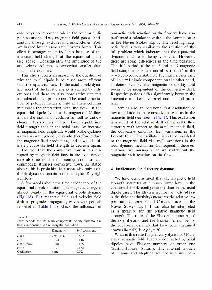
A few words about the time dependence of theequatorial dipole solution. The magnetic energy isalmost steady in the equatorial dipole dynamo(Fig. 1d). But magnetic ¢eld and velocity ¢elddrift as prograde-propagating waves with periodsreported in Table 1. To check the in£uences of

magnetic back reaction on the £ow we have alsoperformed a calculation without the Lorentz forcein the Navier^Stokes Eq. 1. The resulting mag-netic ¢eld is very similar to the solution of thefull problem which indicates that the equatorialdynamo is close to being kinematic. However,there are some di¡erences in the time behavior.The drift period of the m=5 and m=7 magnetic¢eld components is determined by the drift of them=6 convective instability. The much slower driftof the m=1 dipole component, on the other hand,is determined by the magnetic instability andseems to be independent of the convective drift.Respective periods di¡er signi¢cantly between thekinematic (no Lorentz force) and the full prob-lem.

There is also an additional fast oscillation oflow amplitude in the convective as well as in themagnetic ¢eld (see inset in Fig. 1). This oscillationis a result of the relative drift of the m=6 £owstructure with respect to the m=1 magnetic ¢eld,the convective columns ‘feel’ variations in theLorentz force. The oscillation is in turn translatedto the magnetic ¢eld via small variations in thelocal dynamo mechanism. Consequently, these os-cillations are missing when we switch out themagnetic back reaction on the £ow.

4. Implications for planetary dynamos

We have demonstrated that the magnetic ¢eldstrength saturates at a much lower level in theequatorial dipole con¢gurations than in the axialdipole cases. The Elsasser number 1=cB2/b6 (cis the £uid conductivity) measures the relative im-portance of Lorentz and Coriolis forces in theNavier^Stokes Eq. 1. It can also be interpretedas a measure for the relative magnetic ¢eldstrength. The ratio of the Elsasser number 1a ofthe axial dynamo and the Elsasser 1e number ofthe equatorial dynamo that have been examinedabove (Ra=62) is 1a/1e = 20.

What is this ratio for planetary dynamos? Plan-etary magnetic ¢elds that are dominated by axialdipoles have Elsasser numbers of order one(Earth, Jupiter, Saturn). The internal modelsof Uranus and Neptune are not very well con-

Table 1Drift periods for the main components of the dynamo, the£ow component and the energetic oscillation

Kinematic Self-consistent

m=1 2.98W 0.4 0.682m=5 0.124 0.116m=6 (£ow) 0.148 0.135m=7 0.171 0.152Oscillation none 0.023



strained yet. For example, it is still unknownwhere the dynamo region is located. The surface¢elds of Uranus and Neptune are about as largeas the geomagnetic surface ¢eld, we simply as-sume here the ¢elds in the dynamo region arealso of comparable magnitude. The electrical con-ductance in the interior of Uranus and Neptune ismost likely carried by water and ammonia ions.Ab-initio calculations suggest conductivities of theorder 104 S/m [13]. These estimates give an Elsass-er number of order 1032. We thus arrive at a ratio1a/1e of order 102 for the planetary dynamos inour solar system.

The dynamo models explored here suggest thatthe lower ¢eld strength in the equatorial dipolecon¢gurations is a consequence of the mainlytransverse ¢eld lines that oppose the shearing mo-tion of axial vorticity columns. This can possiblyby generalized to all dynamos in rapidly rotatingsystems whose dipole axis is signi¢cantly tiltedaway from the rotation axis. We therefore pro-pose that the anticipated lower Elsasser numbersfor Uranus and Neptune are likely and that thisfact is strongly related to the inclination of themagnetic dipole axes.

Acknowledgements

J.A. acknowledges support through a EuropeanCommunity Marie Curie Fellowship under con-tract number HPMF-CT-2001-01364 during theresearch phase of this work. J.W. has been sup-ported by the German Science Foundation withinthe Scienti¢c Priority Program ‘Geomagnetic Var-iations’. The authors thank Peter Olson and ananonymous referee for comments which substan-tially improved this study.[VC]

References

[1] R. Holme, J. Bloxham, The magnetic ¢eld of Uranus andNeptune: Methods and models, J. Geophys. Res. 101(1996) 2177^2200.

[2] D. Gubbins, C.N. Barber, S. Gibbons, J.J. Love, Kine-matic dynamo action in a sphere, II. Symmetry selection,Proc. R. Soc. Lond. A 456 (2000) 1669^1683.

[3] R. Stieglitz, U. Mu«ller, Experimental demonstration ofthe homogeneous two-scale dynamo, Phys. Fluids 1(2001) 561^564.

[4] G.A. Glatzmaier, P.H. Roberts, A three dimensional selfconsistent computer simulation of the geomagnetic ¢eldreversal, Nature 377 (1995) 203^209.

[5] W. Kuang, J. Bloxham, An Earth-like numerical dynamomodel, Nature 389 (1997) 371^374.

[6] P. Olson, U. Christensen, G.A. Glatzmaier, Numericalmodelling of the geodynamo: Mechanisms of ¢eld gener-ation and equilibration, J. Geophys. Res. 104 (1999)10383^10404.

[7] N. Ishihara, S. Kida, Equatorial magnetic dipole ¢eldintensi¢cation by convection vortices in a rotating spher-ical shell, Fluid Dyn. Res. 31 (2002) 253^274.

[8] E. Grote, F.H. Busse, A. Tilgner, Convection-drivenquadrupolar dynamos in rotating spherical shells, Phys.Rev. E 60 (1999) R5025^R5028.

[9] J. Wicht, Inner-core conductivity in numerical dynamosimulations, Phys. Earth Planet. Int. 132 (2002) 281^302.

[10] C. Kutzner, U. Christensen, From stable dipolar to re-versing numerical dynamos, Phys. Earth Planet. Int. 131(2002) 29^45.

[11] A. Kageyama, T. Sato, Velocity and magnetic ¢eld struc-tures in a magnetohydrodynamic dynamo, Phys. Plasmas4 (1997) 1569^1575.

[12] J. Aubert, N. Gillet, P. Cardin, Quasigeostrophic modelsof convection in rotating spherical shells, Geophys. Geo-chem. Geosyst. 4, doi: 10.1029/2002GC000456.

[13] C. Cavazzoni, G.L. Chiarotti, S. Scandolo, E. Tosatti, N.Bernasconi, N. Parrinello, Superionic and metallic statesof water and ammonia at giant planet conditions, Science283 (1999) 44^46.



Date post:	01-Nov-2016
Category:	Documents
Upload:	julien-aubert
View:	218 times
Download:	2 times

Axial vs. equatorial dipolar dynamo models with implications for planetary magnetic fields

Documents