Axisymmetric Acoustic Scattering by Interpolation Master’s Thesis, Program in Scientific Computing 1 May 2001 Perrin S. Meyer Courant Institute of Mathematical Sciences, New York University, NY. E-mail: [email protected]We describe and implement a numerical method for the solution of an integral equation arising from the exterior Neumann problem for the Helmholtz equation outside an axisymmetric, doubly connected domain in R 3 . The application is the study of acoustic wave propagation through waveguides such as musical horns. Key Words: Helmholtz, waveguide, axisymmetric, horn CONTENTS 1. Introduction. 2. Acoustic Background. 3. Statement of Problem. 4. Axisymmetric Formulation. 5. Solutions based on Single and Double Layer Potential Theory. 6. Numerical Solution of the Exterior Neumann Problem in R 2 . 7. Singularities in the Axisymmetric Kernel. 8. Obstacle Scattering By Interpolation. 9. Numerical Results in R 3 – Scattering off Sound–Soft and Sound–Hard Spheres. 10. Axisymmetric Scattering by Interpolation. 11. Numerical Results of Axisymmetric Scattering by Interpolation. 12. Conclusion. 1. INTRODUCTION We are interested in the study of how sound propagates through musical horns, for example, a trumpet. In this paper we describe a simple, high-order numeri- cal method for the simulation of sound wave propagation through axisymmetric, sound–hard waveguides. The simplest and widely used musical horns are axisym- 1 Advisor: Yu Chen. Reader: Leslie Greengard 1
Transcript
Axisymmetric Acoustic Scattering by Interpolation
Master’s Thesis, Program in Scientific Computing 1
May 2001
Perrin S. MeyerCourant Institute of Mathematical Sciences, New York University, NY.
CONTENTS1. Introduction.2. Acoustic Background.3. Statement of Problem.4. Axisymmetric Formulation.5. Solutions based on Single and Double Layer Potential Theory.6. Numerical Solution of the Exterior Neumann Problem in R2.7. Singularities in the Axisymmetric Kernel.8. Obstacle Scattering By Interpolation.9. Numerical Results in R3 – Scattering off Sound–Soft and Sound–Hard Spheres.10. Axisymmetric Scattering by Interpolation.11. Numerical Results of Axisymmetric Scattering by Interpolation.12. Conclusion.
1. INTRODUCTION
We are interested in the study of how sound propagates through musical horns,for example, a trumpet. In this paper we describe a simple, high-order numeri-cal method for the simulation of sound wave propagation through axisymmetric,sound–hard waveguides. The simplest and widely used musical horns are axisym-
1Advisor: Yu Chen. Reader: Leslie Greengard
1
2 PERRIN S. MEYER
metric, and the underlying mathematical problem is that of obstacle scattering inR3, which we will investigate here.
As is well-known, the axisymmetric problem in R3 can be easily recast as asequence of obstacle scattering problems in R2 by means of the rotational symmetry;therefore the efficiency of a computational scheme is not an issue for medium tohigh frequencies. One of the most efficient mathematical models for the obstaclescattering problem are boundary integral equations based on classical potentialtheory. With this approach, scattering problems of up to 1000 wavelengths (asmeasured in the leading linear dimension) can be solved directly with the currenthardware; this is more than adequate for most applications in the simulation anddesign of acoustic horns.
However, the reduction by rotational symmetry makes the resulting Green’s func-tion extremely complicated in terms of the algebraic structures of its logarithm sin-gularity, which renders existing spectrally convergent quadrature formulae useless.In fact there is no successful effort, to our best knowledge, in addressing this difficultissue of separating the logarithm singularity from the Green’s function to obtain aspectrally convergent quadrature formula for the boundary integral equation.
The solution method we present here avoids the separation of the singularity,and at the same time maintains spectral convergence, all at the expense of a highercondition number of the resulting linear system to be solved. The high conditionnumber does not cause any instability (see Section 8) but the spectral convergencestops when the error drops to about 10−8.
A major advantage of the new approach is the simplicity of coding. There isno need to design quadratures for singular integrals and only discrete points areneeded on the curves and surfaces of the scatterer, not “elements”, or collectionsof low–order spline curves or surfaces.
2. ACOUSTIC BACKGROUNDIf sound waves propagating in air are low intensity, the acoustic propagation of
these waves is well modeled by a linearization of the Euler equations of gas dynamics[19] which results in the linear wave equation
∇2p(x, t)− 1c2∂2p(x, t)∂t2
= 0 (1)
where x is a point in R3, p(x, t) is an acoustic pressure disturbance field, t is time,and c is the speed of sound2. Air does not become appreciably non–linear untilwell above the levels required to produce immediate hearing damage in humans,and so this linearization is valid for sounds created by musical instruments, oreven from sound produced by high–power loudspeakers. c varies with changes inatmospheric pressure, temperature, and humidity, but for small acoustic problemsit can assumed to be constant. Here by “small” we mean sound propagation instill air with distances of less than a hundred meters. The value commonly usedfor room temperature and standard atmospheric pressure is a wave speed of 343meters per second.
2In our notation we will use bold to denote variables that represent points in R3
AXISYMMETRIC ACOUSTIC SCATTERING BY INTERPOLATION 3
Under the standard time-harmonic assumption, and with ω as the angular fre-quency
p(x, t) = Real{u(x)e−iωt} (2)
we find that u satisfies the Helmholtz equation
4u(x) + k2 u(x) = 0 (3)
where k is the wavenumber k = ωc , and ∇2 = 4.
3. STATEMENT OF PROBLEMWe wish to solve an exterior Neumann axisymmetric scattering problem. Given a
continuous function g on ∂D, find a radiating solution u ∈ C2(R3�D)∩C(R3�D)to the Helmholtz equation
4u+ k2u = 0 in R3�D (4)
which satisfies the boundary condition
∂u
∂ν= g on ∂D (5)
in the sense of uniform convergence on ∂D. Let D be a doubly connected domainin R3. We assume the boundary ∂D to be connected and of class C2,β. by ν wedenote the unit normal vector to the boundary ∂D directed to the exterior of D.
4. AXISYMMETRIC FORMULATIONWe are interested in modeling sound waves propagation through an axisymmetric
waveguides in R3. As is well-known, at high frequencies or large k, the computa-tional requirements for the Helmholtz equation are very large. Methods for solvingthe Helmholtz equation based on numerically solving boundary integral equationsproduce large, dense, and complex systems of linear equations that need to besolved, and the linear system is different for every wave number k. Direct meth-ods for even medium size k can produce dense matrices on the order of 30,000by 30,000, requiring tens of Gigabytes of main memory storage, and hundreds ofhours of computer time [5]. Even if iterative methods are used [20], the storage andcomputational costs are enormous. Efficient numerical methods are still an activeresearch topic [4, 9, 23, 24, 6, 22, 14]. The Fast Multipole Method (FMM) can re-duce the storage costs from n2 (where n is the number of points or elements used todiscretize the scatterer) to O(n log2 n) and the computational costs to O(n log2 n).Unfortunately, a multilevel adaptive FMM for the Helmholtz equation is extremelydifficult to code, and to our knowledge, there are no free or open–source implemen-tations currently available.
However, an axisymmetric obstacle scattering problem in R3, which we will in-vestigate, can easily be reduced to a sequence of obstacle scattering problems inR2; therefore the issue of efficiency is minimal. In fact, such a scattering problemcan be solved up to size 1000 wavelengths on current workstations.
The following equations describe our axisymmetric formulation. Let x, y, z denotethe Cartesian coordinate system. If x(t) is the x component of a simple curve
4 PERRIN S. MEYER
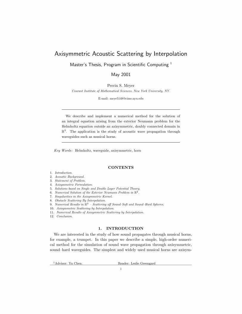
FIG. 1. This figure shows a rendering of a green torus. The red sphere shows the location ofthe point source creating an incident sound field.
parameterized by t, and y(t) is the y component of the same curve parameterizedby t, then if we rotate this curve around the x axis, the equation for the scatteringsurface y(t, θ) (denoted by ∂D, and parameterized by t and θ) described by thisrotation is
y(t, θ) = x(t)x+ y(t) cos(θ)y + y(t) sin(θ)z (6)
For example, if x(t) = 3+cos(t) and y(t) = 3+sin(t), 0 ≤ t ≤ 2π, the surface–of–rotation ∂D is the green torus shown in figure 1. The red sphere shows the locationof a point source that creates the incident scattering field.
5. SOLUTIONS BASED ON SINGLE AND DOUBLE LAYERPOTENTIAL THEORY
Because we are interested in homogeneous free–space scattering, it is natural torecast the Helmholtz equation into a boundary integral formulation on the surfaceof the scatterer ∂D.
Colton and Kress [10] describe a solution of the exterior Neumann Helmholtzequation by using a combined single and double layer approach from potentialtheory.
We seek solutions in the form
u(x) =∫
∂D
(Φ(x,y)ϕ(y) + iη
∂Φ(x,y)∂ν(y)
ϕ(y))ds(y), x /∈ ∂D (7)
with continuous density ϕ and a real coupling parameter η 6= 0. Equation (7) solvesthe exterior Neumann problem provided the density is a solution to the second–kindintegral equation
ϕ−K ′ϕ− iηTϕ = −2g (8)
AXISYMMETRIC ACOUSTIC SCATTERING BY INTERPOLATION 5
where the integral operators K ′ and T are
(K ′ϕ)(x) = 2∫
∂D
∂Φ(x,y)∂ν(x)
ϕ(y) ds(y) x ∈ ∂D (9)
(Tϕ)(x) = 2∂
∂ν(x)
∫∂D
∂Φ(x,y)∂ν(y)
ϕ(y)ds(y), x ∈ ∂D (10)
This solution is unique for all (positive) wavenumbers k. If the coupling parameteris chosen to be η = 0, then the single layer formulation is non-unique when k2 isan interior Dirichlet eigenvalue of −4, often known as an “internal resonance.”
We note that technical difficulties arise when implementing a numerical methodbased on equation (8) because of the hypersingular operator T . Kress [16] describesa method attributed to Maue that can be used to overcome this difficulty.
Grannel et. al. [13] describe a method first proposed in the acoustics literatureby Burton that uses a combination of only weakly singular integral operators. K ′
where the zero subscript on an operator signifies that operator in the “static” limitk = 0.
6. NUMERICAL SOLUTION OF THE EXTERIOR NEUMANNPROBLEM IN R2
Kress [16] describes a numerical method for the solution of the exterior Neumannproblem in R2 (cylindrical scattering). It solves the second–kind integral equation(8) using a Nystrom method on analytic boundary curves described by trigonomet-ric interpolating polynomials. By properly treating the logarithmic singularity inthe fundamental solution of the Helmholtz equation in R2, the method achievessuperalgebraic convergence for analytic boundary curves.
We had originally hoped to modify this method for the solution of our axisym-metric scattering problem, because by assuming axisymmetric symmetry, we are ineffect reducing our scattering problem in R3 to a one dimensional boundary inte-gral in R2. The axisymmetric kernel has a logarithmic singularity, but we foundit impossible to find a suitable splitting of the axisymmetric kernel in the formln(kR(x,y))K1(x,y) + K2(x,y) in order to use the Nystrom method. We sketchthe method because of its elegance and in the hope that someone will direct us toa suitable splitting that would allow us to use this method on our axisymmetricscattering problem.
In two dimensions, the fundamental solution to the Helmholtz equation is
Φ(x, y) :=i
4H
(1)0 (κ|x− y|), x 6= y (14)
6 PERRIN S. MEYER
where Hn is a Hankel function of the first kind of order n (see [10, 1]).
H(1,2)n := Jn ± iYn (15)
where Jn are Bessel functions of order n
Jn(t) :=∞∑
p=0
(−1)p
p!(n+ p)!
(t
2
)n+2p
(16)
and Yn are Neumann functions of order n
Yn(t) :=2π{ln t
2+ C}Jn(t)− 1
π
n−1∑p=0
(n− 1− p)!p!
(2t
)n−2p
− 1π
∞∑p=0
(−1)p
p!(n+ p)!
(t
2
)n+2p
{ψ(p+ n) + ψ(p)} (17)
Kress assumes the that the boundary curve ∂D possesses a regular analytic and2π periodic parametric representation of the form
x(t) = (x1(t), x2(t)), 0 ≤ t ≤ 2π (18)
in a counterclockwise orientation satisfying [x′1(t)]2 + [x′2(t)]
After some algebra, we can reduce this equation to the form
ψ(t)−∫ 2π
0
K(t, τ)ψ(τ)dτ = g(t), 0 ≤ t ≤ 2π (21)
K(t, τ) =i κH
(1)1 (κ r(t, τ))2 r(t, τ)
{x′2(t)[x1(τ)− x1(t)]− x′1(t)[x2(τ)− x2(t)]}
{[x′1(τ)]2 + [x′2(τ)]2} 1
2
{[x′1(t)]2 + [x′2(t)]2}12
(22)
If we split the kernel K into two parts
K(t, τ) = K1(t, τ) ln(
4 sin2 t− τ
2
)+K2(t, τ) (23)
AXISYMMETRIC ACOUSTIC SCATTERING BY INTERPOLATION 7
K1(t, τ) =−k2π
J1(k r(t, τ))r(t, τ)
{x′2(t)[x1(τ)− x1(t)]− x′1(t)[x2(τ)− x2(t)]}
{[x′1(τ)]2 + [x′2(τ)]2} 1
2
{[x′1(t)]2 + [x′2(t)]2}12
(24)
K2(t, τ) = K(t, τ)−K1(t, τ) ln(
4 sin2 t− τ
2
)(25)
K1 and K2 are analytic, and the diagonal terms are
K2(t, t) = K(t, t) =12π
x′2(t)x′′1(t)− x′1(t)x
′′2(t)
[x′1(t)]2 + [x′2(t)]2(26)
(and K1 = 0). The Nystrom method consists in the straightforward approximationof the integrals by quadrature formulas. For the 2π periodic integrands, we choosean equidistant set of knots
tj :=πj
n, j = 0, . . . , 2n− 1, (27)
and the quadrature rule∫ 2π
0
ln(
4 sin2 t− τ
2
)f(τ)dτ ≈
2n−1∑j=0
R(n)j (t)f(tj), 0 ≤ t ≤ 2π (28)
with the quadrature weights given by
R(n)j (t) := −2π
n
n−1∑m=1
1m
cosm(t− tj)−π
n2cosn(t− tj), j = 0, . . . , 2n− 1,
and the trapezoidal rule ∫ 2π
0
f(τ)dτ ≈ π
n
2n−1∑j=0
f(tj) (29)
Both these numerical integration formulas are obtained by replacing the integrandf by its trigonometric interpolation polynomial and then integrating exactly. In theNystrom method, the integral equation is replaced by the approximating equation
ψ(n)(t)−2n−1∑j=0
{R(n)j (t)K1(t, tj) +
π
nK2(t, tj)}ψ(n)(tj) = g(t) (30)
(3.72) reduces to solving a linear system of equations
ψ(n)i −
2n−1∑j=0
{R(n)|i−j|K1(ti, tj) +
π
nK2(ti, tj)}ψ(n)
j = g(ti) (31)
for i = 0, 1, . . . , 2n− 1, where
R(n)j := R
(n)j (0) = −2π
n
n−1∑m=1
1m
cosmjπ
n− (−1)jπ
n2, j = 0, . . . , 2n− 1, (32)
8 PERRIN S. MEYER
7. SINGULARITIES IN THE AXISYMMETRIC KERNELIn order to solve the three dimensional axisymmetric scattering problem, we
need an an expression for the axisymmetric free space Green’s function. x and yare points in R3 on the surface of rotation ∂D. In order to keep the notation similarto the discussion of the Nystrom method in R2, we will again parameterize our twodimensional boundary curve with trigonometric interpolating polynomials x and yindexed by t and τ , but with the additional variables θt and θτ which describe angleof the surface of rotation. x and y are then defined as
For simplicity in notation, and to be consistent with [13, 18], we introduce thefunctions a(t, τ) and b(t, τ), and from simple trigonometric reduction derive anexpression for R(x,y) for x and y on ∂D
If we assume that our boundary conditions are also axisymmetric g(t, θt) =g(t, 0), then for our axisymmetric horn the surface integral operators are effec-tively replaced with one-dimensional integral operators over ∂D. Recall that thefree space Green’s function for the Helmholtz equation in R3 is
Φ(x,y) =14π
eikR
R(39)
Because R now only depends on R(t, τ, θ), we obtain axisymmetric kernels of theform
K(t, τ) =14π
∫ 2π
0
ei k R
Rdθ (40)
When t = τ and θ = 0, the kernel in equation (40) becomes singular, and inorder to solve the boundary integral equation numerically the singularity must bedealt with.
For our first attempt at treating the singularity in the axisymmetric kernel, wefollowed a suggestion from [13]. They described a method where they subtract outthe
∫1R logarithmic singularity (which is static, i.e. not dependent on k):∫ 2π
o
eikR
R=∫ 2π
o
eikR − 1R
+∫ 2π
o
1R
(41)
AXISYMMETRIC ACOUSTIC SCATTERING BY INTERPOLATION 9
After suitable manipulation, this equation can be recast as a hypergeometric series.From [1, 13, 12, 17],
∫ 2π
01R d θτ is a complete elliptic integral of the first kind Ke(m)
which can be written as a hypergeometric series H(α, β; c; z)∫ 2π
From these equations, we can write an explicit expression for the logarithmic sin-gularity
ln(a(t, τ)− b(t, τ))
(2L(t)
π√a(t, τ) + b(t, τ)
) ∞∑n=0
(Γ(n+ 1
2 )n!
)2(a(t, τ)− b(t, τ)a(t, τ) + b(t, τ)
)n
︸ ︷︷ ︸K1(t,τ)
(51)Unfortunately, this singularity extraction does not completely treat the logarith-
mic singularity, as noted [5, 4], because the derivatives of eikR−1R are unbounded.
This would limit the convergence of the previously described Nystrom method toa low order method.
Kress directed us to paper he had written about the magnetic confinement ofan electrically conducting fluid in a torus (with applications in fusion research)[15],which happens to have the same form as our exterior Neumann axisymmetric scat-tering problem. In this paper, he includes a more involved procedure in order totreat the logarithmic singularity: “For a satisfactory numerical approximation acareful investigation of the nature of the singularity of the kernels is necessary.Since essentially we are solving a two-dimensional boundary–value problem in the
10 PERRIN S. MEYER
cross–section of ∂D we expect a logarithmic singularity when t = τ .” Here, hedefines (for integers m) the integrals
Im(t, τ) =∫ 2π
0
[R(t, τ, θ)]m−1dθ (52)
and
Jm(t, τ) =∫ 2π
0
cos(θ)[R(t, τ, θ)]m−1dθ (53)
where R(t, τ, θ) are as defined in (38) (with θτ = 0). Through partial integration,Kress introduces the recurrence equations
Im+2 = pIm − qJm (54)
and
(m+ 3)Jm+2 = (m+ 1)[pJm − qIm] (55)
where for even indices the initial terms are given through
I0 =4
(p+ q)12K(k) (56)
and
J0 =4
q(p+ q)12[pK(k)− (p+ q)E(k)] (57)
where
p(t, τ) = [y(t)]2 + [y(τ)]2 + [x(t)− x(τ)]2
and
q(t, τ) = 2y(t)y(τ)
where
k(t, τ) =(
2q(t, τ)p(t, τ) + q(t, τ)
) 12
and E and K denote the complete elliptic integrals
E(k) =∫ 2π
0
(1− k2 sin2(θ))12 dθ
K(k) =∫ 2π
0
(1− k2 sin2(θ))−12 dθ
After a few more pages of manipulation of this sorts he arrives at a suitable splittingof the axisymmetric kernels in the form ln(Ks(t, τ))K1(t, τ) + K2(t, τ), where foranalytic boundary cross sections of the torus the kernels K1 and K2 are analytic.He then uses the exact same Nystrom quadrature method with trigonometric in-terpolation polynomials as described above for the R2 case to solve the boundaryintegral equations in this axisymmetric setting.
AXISYMMETRIC ACOUSTIC SCATTERING BY INTERPOLATION 11
Unfortunately, as he states on page 337: “Note that equations (54) and (55) areunstable, but they can be transformed into recurrence relations for Im = km
m! Im andJm = km
m! Jm which turn out to be stable for k not too large.” Also unfortunately,he gives no estimate of what “too large” is.
We found in our own numerical tests that this recursion scheme is unstable (indouble precision) for ka greater than approximately 5, where a is a characteristiclength scale (1 in our tests). This would limit the usefulness of this scheme as anumerical method to only low frequency scattering problems, despite the high–orderconvergence.
8. OBSTACLE SCATTERING BY INTERPOLATIONBecause of the difficulties in finding a suitable splitting of the logarithmic singu-
larity in the axisymmetric formulation, we decided to develop a numerical solutionmethod based on solving a first–kind integral equation by interpolation. In thisformulation, the points x and y never coincide, and the kernels are thus never sin-gular. The following method is based on a seminar given on 9 October 2000 at theCourant Institute, presented by Yu Chen.[8]
We note that many others have solved Helmholtz scattering problems by solvinga first–kind integral equation. In the literature, this has been called a “Null Field”or “T–matrix” method, for example. A recent review summarizes these methodsunder the name “discrete source” methods [11].
Our method is described below.We assume that the obstacleD is surrounded by a homogeneous medium, referred
to as the free space.We will adopt the point of view that a wave, incident or scattered, is generated
by its sources: (i) The incident wave u0 by sources outside D (ii) The scatteredwave v by sources on the scattering surface ∂D.
For simplicity, we assume that the incident wave is generated by a point sourceat x0 outside D,
u0(x) =14π
eik|x−x0|
|x− x0|x 6= x0 (58)
Outside the support of its sources, a time–harmonic wave w in free space satisfiesthe Helmholtz equation
4w(x) + k2w(x) = 0 (59)
where k = ωc is the wavenumber, ω is the temporal frequency, and c is the wave
speed.Therefore, outside D, the incident and scattered waves uo, v satisfy
4u0(x) + k2u0(x) = δ(x− x0) (60)
4v(x) + k2v(x) = 0 (61)
and u(x) = u0(x) + v(x) is the total field, representing pressure at x.The mechanical and physical properties of the obstacle surface ∂D determine the
boundary conditions for v(1) Soft boundary – pressure vanishes: u0 + v = 0 (Dirichlet)
12 PERRIN S. MEYER
(2) Hard boundary – displacement vanishes: ∂(u0+v)∂n = 0 (Neumann)
n is the outward unit normal of ∂DWe therefore have Dirichlet or Neumann boundary conditions for the scattered
field v on ∂D
4v(x) + k2v(x) = 0, x ∈ R3 � D (62)
v = −u0 or∂v
∂n= −∂u0
∂nx ∈ ∂D (63)
Together with the Sommerfeld radiation condition
limr→∞
r
(∂u
∂r− iku
)= 0 r = |x| (64)
both these boundary value problems are well–posed, and uniquely determines vfrom the incident field u0 on ∂D.
In the approach of the Helmholtz equation or boundary integral equation, it isalways the knowledge of the incident field u0 on the boundary ∂D that uniquelydetermines the scattered field. The interior D is of no concern to us, and thescattering problem is never defined inside D. We wish to explore the interior of Dby re–interpreting the scattering problem in the interior.
For simplicity, we assume that the wave number k is not an interior Dirichlet orNeumann eigenvalue, and that ∂D is smooth.
Let us forget for a moment the original scattering problem by assuming thatthere is no obstacle in D. Then the whole space becomes free space in and outsideD. Except at x0, the incident field u0 is well–defined everywhere, particularly in D.Under the conditions that k is not an interior Dirichlet eigenvalue, it is well–knownthat there exists a unique, smooth distribution α of monopole sources on ∂D whosepotential matches u0 inside D:
u0(x) =∫
∂D
G(x,y)α(y)ds x ∈ D (65)
where for 3–D
G(x,y) = Φ(x,y) =14π
eik|x−y|
|x− y|(66)
We will refer to the point source at x0 outside D which generates the incident fieldu0 as the primary source, and the monopole sources α on ∂D as the equivalent orsecondary sources. To an observer in D, the primary and secondary sources lookidentical (or sound identical for acoustic waves).
Similarly, under the condition that k in not an interior Neumann eigenvalue, thereexists a unique, smooth distribution β of dipole sources on ∂D whose potentialmatches u0 inside D:
u0(x) =∫
∂D
∂G(x,y)∂n(y)
β(y)ds, x ∈ D (67)
The two obstacle scattering problems with Dirichlet and Neumann boundaryconditions are equivalent to the determination of the equivalent (secondary) sourcesof monopoles or dipoles.
AXISYMMETRIC ACOUSTIC SCATTERING BY INTERPOLATION 13
Theorem. Let k be not an eigenvalue and ∂D smooth. then(i) v defined by the formula
v(x) = −∫
∂D
G(x,y)α(y)ds, x ∈ R3 �D (68)
is a solution of the Dirichlet problem(ii) v defined by the formula
v(x) = −∫
∂D
∂G(x,y)∂n(y)
β(y)ds, x ∈ R3 � D (69)
is a solution of the Neumann problem.Solving the obstacle scattering problem is equivalent to finding the secondary
sources on ∂D. In order to find the secondary sources by interpolation, we need todefine Γ, a smooth, closed curve in D, parallel and sufficiently close to ∂D. Thesecondary sources we seek then satisfy the equation
u0(x) =∫
∂D
G(x,y)α(y) ds, x ∈ Γ (70)
for the Dirichlet case and
u0(x) =∫
∂D
∂G(x,y)∂n(y)
β(y)ds, x ∈ Γ (71)
for the Neumann case.To determine α or β, a first kind integral equation has to be solved. There are
advantages and disadvantages in treating a first kind integral equation numerically.We will first discuss the advantages and then consider ways to to minimize thedrawbacks. The main advantage is that the kernels are not singular – there isno need to design quadratures for singular integrals. As we have noted, even if wehave available quadratures for singular integrals, it requires knowledge of the kernelK(x,y) = g(x,y) s(x,y) + h(x,y), (where s(x,y) is singular when x = y and g
and h are smooth) which may not be available.In order to solve, e.g., the integral equation
u0(x) =∫
∂D
G(x,y)α(y) ds, x ∈ Γ (72)
it seems that we need to discretize the integral by quadrature. Instead, we maychange our point of view, and there is no need to design quadrature at all – thequadrature issue can be replaced by interpolation. Why interpolation? For sim-plicity, we assume that the primary sources are monopoles located on Σ which isseparated from ∂D by a distance d – the linear map A : C(Σ) → C(D) defined bythe formula
u0(x) = (Aη)(x) =:∫
Σ
G(x,y)η(y) ds, x ∈ D (73)
maps the primary source η to its incident field u0, and is a compact linear operator,with singular values decaying exponentially to zero. For a given precision ε, the
14 PERRIN S. MEYER
numerical rank of A is finite and proportional to | log(ε)|. This rank(A) is thenumber of degrees of freedom to specify, to the same precision, an arbitrary incidentfield u0 in D generated by source η on Σ. Therefore, the task of finding the secondarysources on ∂D to match u0 in D to precision ε becomes an issue of matching theserank(A) parameters which specify u0 in D.
Algorithm for Obstacle Scattering by Interpolation
• Choose n equispaced points {yj} on ∂D as the locations of the secondarypoint sources, with h as the sampling interval.
• Choose the parallel curve or surface Γ in D that is separated from ∂D by aconstant multiple of h.
• Place m equispaced points {xi} on Γ to sample uo.
• Solve the m–by–n linear system with m ≥ n
u0(xi) =n∑
j=1
G(xi,yj)αj , i = 1, 2, . . .m (74)
for the Dirichlet case or
u0(xi) =n∑
j=1
∂G(xi,yj)∂n(yj)
βj , i = 1, 2, . . .m (75)
for the Neumann case as a least–squares problem.
This is a standard least–squares problem for interpolation with basis functionsbj(x) = G(x,y) and interpolation points xi.
The points {xi} and {yj} do not have to be equispaced, and there is no need forquadrature weights.
The solution {αj} or {βj} is not an approximation to {α(yj)} or {β(yj)} – it ismore likely to be {α( yj)wj} or {β(yj)wj} where wj are some sort of (unknown)quadrature weights.
Interpolation is not sensitive to the complication of geometry, and computercoding in two and three dimensions is simple.
The main drawback of this approach is ill-conditioning. For a fixed location ofΓ, the m–by–n linear system becomes exponentially ill–conditioned as m and n
increase. As a compromise, it turns out that in double precision of 16 digits, aseparation of the testing locations on Γ from sources on ∂D by 3 to 4 h is ideal tobalance conditioning and accuracy. h is the distance between the sources on ∂D.The numerical rank of the m–by–n linear system for a condition number of 108
grows linearly with n, and the scattered field v has about 8 correct digits.
AXISYMMETRIC ACOUSTIC SCATTERING BY INTERPOLATION 15
9. NUMERICAL RESULTS IN R3 – SCATTERING OFFSOUND–SOFT AND SOUND–HARD SPHERES
As a first test of our numerical method, we will compute the scattering off sound–soft and sound–hard spheres. This is a good test, because we have an exact ana-lytical series solution to compare against.
The exact solution [3] of an incident wave V i created by a point source at r0 =(r0, 0, 0) such that V i = eikR
kR scattering off a sound soft sphere is given by :
V i + V s = i∞∑
n=0
(2n+ 1)Pn(cos θ)h(1)n (kr>)[jn(kr<)− jn(ka)
h(1)n (ka)
h(1)n (kr<)] (76)
Where jn,h(1)n , and Pn are spherical Bessel, spherical Hankel, and Legendre func-
tions as defined in [1]:
jn(x)=√
π
2xJn+ 1
2(x) (77)
h(1)n (x)=
√π
2xH
(1)
n+ 12(x) (78)
and a is the radius of the sphere.The exact solution of a point source scattering off a sound hard sphere is:
V i + V s = i
∞∑n=0
(2n+ 1)Pn(cos θ)h(1)n (kr>)[jn(kr<)− j′n(ka)
h(1)′n (ka)
h(1)n (kr<)] (79)
Where the ′ denotes the derivative:
j′n(x) = −1/4√
2Jn+ 12(x)π
1√πx
x−2 + 1/2√
2√π
x(−Jn+ 3
2(x) +
(n+ 1/2) Jn+ 12(x)
x
)(80)
h(1)′
n (x) = −1/4√
2H(1)
n+ 12(x)π
1√πx
x−2 + 1/2√
2√π
x−H(1)
n+ 32(x) +
(n+ 1/2)H(1)
n+ 12(x)
x
(81)
These equations were computed in Matlab to machine precision ( 10−16).Our scattering surface ∂D is a sphere of radius 1 centered at the origin (0, 0, 0).
In order to implement our interpolation method, we need to place n equispacedpoints {yj} on ∂D as locations of the secondary sources, and m points {xi} on thesurface of the the smaller sphere Γ inside D of radius rΓ as the testing locations. Inorder to do so, we create an algorithm that places points spaced approximately hapart in both longitude and latitude. This quasi-uniform spacing was used for both
16 PERRIN S. MEYER
the location of the secondary sources {yj} on ∂D and the location of the samplingpoints {xi} on the sphere Γ, also located at the origin, but with a radius 1− 3h.
The interpolation algorithm was coded in ANSI C. The results in Table 1–2 andFigure 2 were obtained on a Pentium II 266MHz PC running Linux and compiledusing GCC3, while the results in Figure 3 were obtained on an Sun Ultra–80 work-station using the Sun C compiler. In both cases the LAPACK[2] complex SVDbased least–squares routine ZGELSS was used to solve the linear system. UnderLinux, good performance was obtained by utilizing the BLAS from the ATLASproject 4. Matlab 5 was used to compute the analytic series solution, as well as forvisualization.
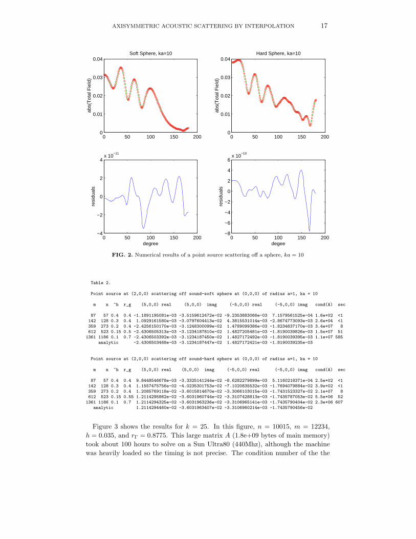
Table 1 shows numerical convergence results for k = 5. The point source islocated at (2, 0, 0), and the measurement locations are at (5, 0, 0) (the backscatteredwave) and (−5, 0, 0) (the shadow region). The total field V i + V s is shown. r g isrΓ, the radius of the inner surface Γ. sec represents the wall clock running time ofthe code, rounded to the nearest second. The last line of the table shows the resultof equations (76) and (79).
Table 1.
Point source at (2,0,0) scattering off a sound-soft sphere at (0,0,0) of radius a=1, ka = 5
m n ~h r_g (5,0,0) real (5,0,0) imag (-5,0,0) real (-5,0,0) imag cond(A) sec
Table 2 shows the convergence results for k = 10. Note the high order convergenceis clearly visible – as n is approximately doubled from 273 to 523 the number ofcorrect digits approximately doubles. Figure 2 shows a plot of 00 → 1800 at radius5, with the lower plot showing the residuals between the numerical method and andthe analytical series solution (although the magnitude of the complex total field isplotted), different from the real and imaginary results presented in Table 1).
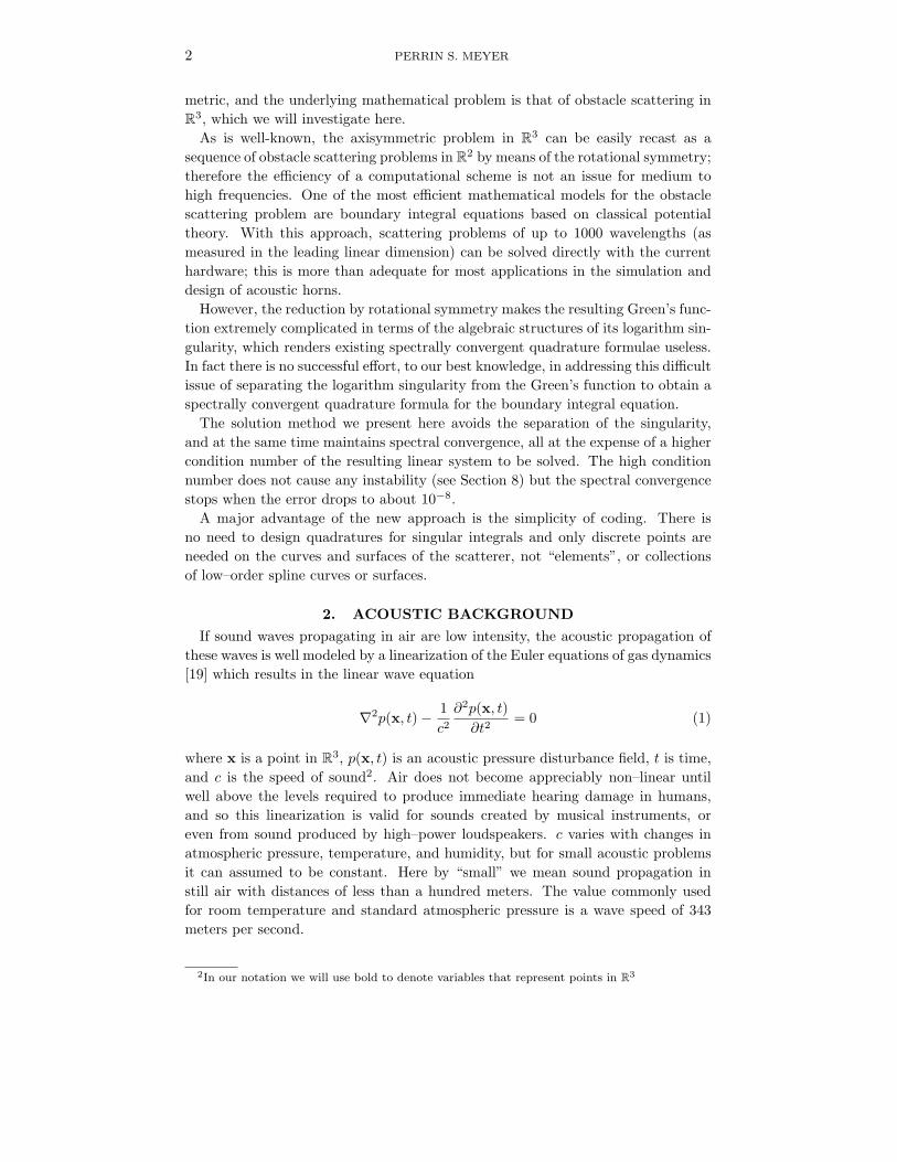
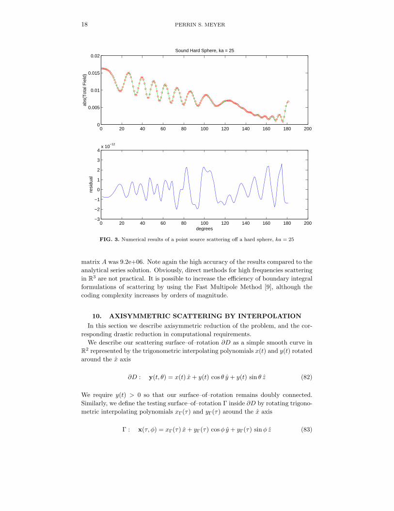
Figure 3 shows the results for k = 25. In this figure, n = 10015, m = 12234,h = 0.035, and rΓ = 0.8775. This large matrix A (1.8e+09 bytes of main memory)took about 100 hours to solve on a Sun Ultra80 (440Mhz), although the machinewas heavily loaded so the timing is not precise. The condition number of the the
18 PERRIN S. MEYER
0 20 40 60 80 100 120 140 160 180 2000
0.005
0.01
0.015
0.02Sound Hard Sphere, ka = 25
abs(
Tot
al F
ield
)
0 20 40 60 80 100 120 140 160 180 200−3
−2
−1
0
1
2
3
4x 10
−12
res
idua
l
degrees
FIG. 3. Numerical results of a point source scattering off a hard sphere, ka = 25
matrix A was 9.2e+06. Note again the high accuracy of the results compared to theanalytical series solution. Obviously, direct methods for high frequencies scatteringin R3 are not practical. It is possible to increase the efficiency of boundary integralformulations of scattering by using the Fast Multipole Method [9], although thecoding complexity increases by orders of magnitude.
10. AXISYMMETRIC SCATTERING BY INTERPOLATION
In this section we describe axisymmetric reduction of the problem, and the cor-responding drastic reduction in computational requirements.
We describe our scattering surface–of–rotation ∂D as a simple smooth curve inR2 represented by the trigonometric interpolating polynomials x(t) and y(t) rotatedaround the x axis
∂D : y(t, θ) = x(t) x+ y(t) cos θ y + y(t) sin θ z (82)
We require y(t) > 0 so that our surface–of–rotation remains doubly connected.Similarly, we define the testing surface–of–rotation Γ inside ∂D by rotating trigono-metric interpolating polynomials xΓ(τ) and yΓ(τ) around the x axis
Γ : x(τ, φ) = xΓ(τ) x+ yΓ(τ) cosφ y + yΓ(τ) sinφ z (83)
AXISYMMETRIC ACOUSTIC SCATTERING BY INTERPOLATION 19
It is convenient to define a complex function w(t) and the Fourier series
w(t) =∑
Am ei m t (84)
with Fourier coefficients Am so that x(t) is the real component of w(t) and y(t)is the imaginary component of w(t): w(t) = x(t) + i y(t). Similarly, we define thecomplex function wΓ(t) and the Fourier series
wΓ(τ) =∑
Bm ei m τ (85)
and the Fourier coefficients Bm to represent xΓ(τ) and yΓ(τ): wΓ(τ) = xΓ(τ) +i yΓ(τ).
The distance between the sources {yj} on the surface ∂D and the points {xi}on the sampling surface Γ is
R(x,y) = |x− y|
=√
(x(t)− xΓ(τ))2 + (y(t) cos θ − yΓ(τ) cosφ)2 + (y(t) sin θ − yΓ(τ) sinφ)2 (86)
If we allow only axisymmetric incident waves (i.e. in our case point sources lo-cated on the x axis), then we can set φ = 0, and sample the sum of our axisymmetricGreens functions (dipole ring sources) only at xi = xΓ(τi) x+yΓ(τi) y. We then getthe interpolation method for axisymmetric exterior sound–hard scattering
u0(xi) =n∑
j=1
∂G(xi,yj)∂n(yj)
βj , i = 1, 2, . . .m (87)
u0(xi) =n∑
j=1
[∫ 2π
0
∇ eikR(xi,yj)
R(xi,yj)· n(yj) dθ
]βj , i = 1, 2, . . .m (88)
where
∇ eikR(xi,yj)
R(xi,yj)· n(yj) =[
i keikR
R2− eikR
R3
][x(tj)− xΓ(τi)]nx(tj) + [y(tj)ny(tj)]− [yΓ(τi)ny(tj) cos θ]
(89)
where nx(tj) is the x component of unit normal n(yj) at point yj on ∂D, andny(tj) is the y component of unit normal n(yj) at point yj on ∂D. Because in ourinterpolation method the surface ∂D with the secondary dipole ring sources {yj}is separated by a constant multiple from the points {xi} on Γ where we sample u0,the integral ∫ 2π
0
∇ eikR(xi,yj)
R(xi,yj)· n(yj) dθ (90)
is never singular, and so we can use a (simple) trapezoidal rule quadrature method(equation (29)) to calculate the entries to the m–by–n matrix A.
20 PERRIN S. MEYER
A similar method can of course be easily developed for sound–soft scattering,but this method was not implemented, as we are primarily interested in sound–hard scattering problems.
11. NUMERICAL RESULTS OF AXISYMMETRIC SCATTERINGBY INTERPOLATION
The previous section verified that the interpolation method provides for high–order convergence for the scattering off spheres in R3. We then used this verifiedcode to solve the axisymmetric scattering problem of a torus (donut). For this test,we put points over the entire surface of the torus in R3, in order to have a resultwith which to compare the axisymmetric reduction.
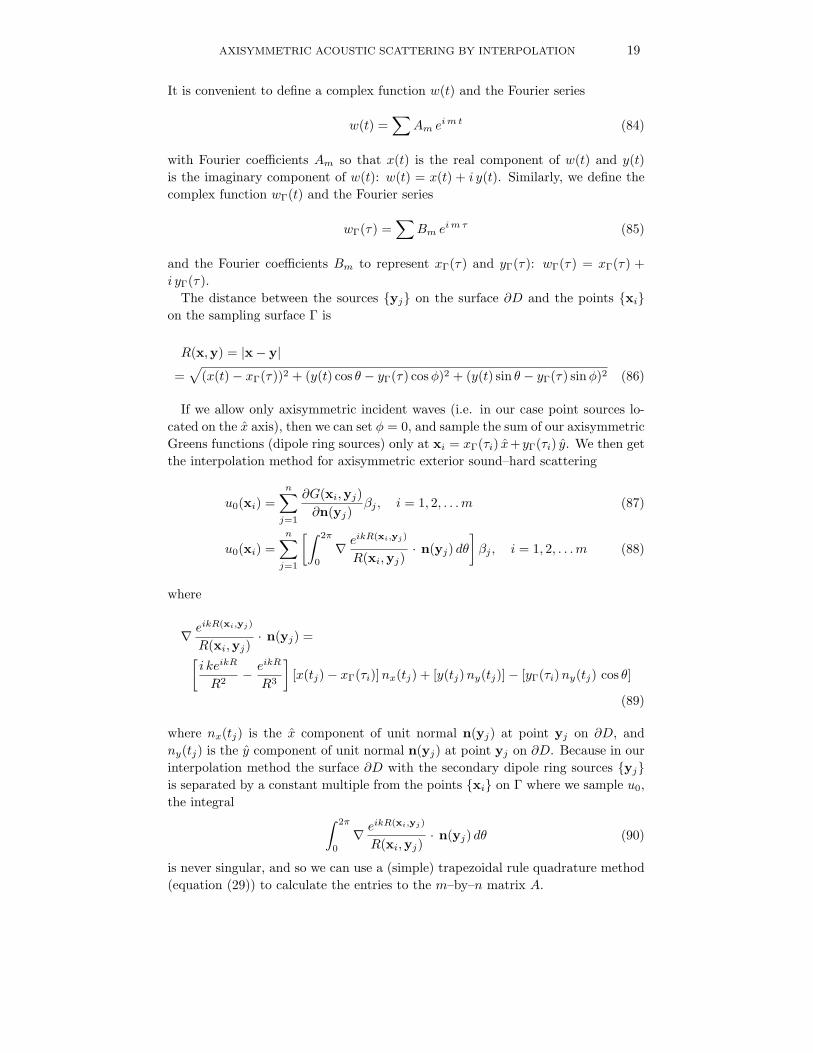
We define the torus as a surface of revolution around the x axis. Figure 4 showsthe 2–D plot of a circle of radius 1 centered at (3, 3, 0). If this circle is rotatedaround the x axis, the torus surface ∂D shown in green in figure 1 is created. (Thered sphere in figure 1 shows the location of the point source creating the incidentfield u0). We place n secondary dipole ring sources {yj} on ∂D and m samplinglocations {xi} on the surface Γ, which is a torus of smaller minor radius rΓ insidethe torus ∂D:
y(t, θ) = (3 + cos t) x+ ((3 + sin t) cos θ) y + ((3 + sin t) sin θ) z (91)
x(τ, φ) = (3 + rΓ cos τ) x+ ((3 + rΓ sin τ) cosφ) y + ((3 + rΓ sin τ) sinφ) z (92)
Table 3 shows the convergence results for the R3 algorithm for an increasing num-ber of points ( and a correspondingly smaller h). The two measurement locationswere (10, 0) and (−10, 0). Note that we get about 5-6 correct digits.
Table. 3.
Point Source Scattering off a Torus
Hard Scattering off a Donut: circle centered at (3,3) with radius 1 rotated around x axis
k = 1 Points in R^3
m n ~h r_g (10,0) real (10,0) imag (-10,0) real (-10,0) imag cond sec
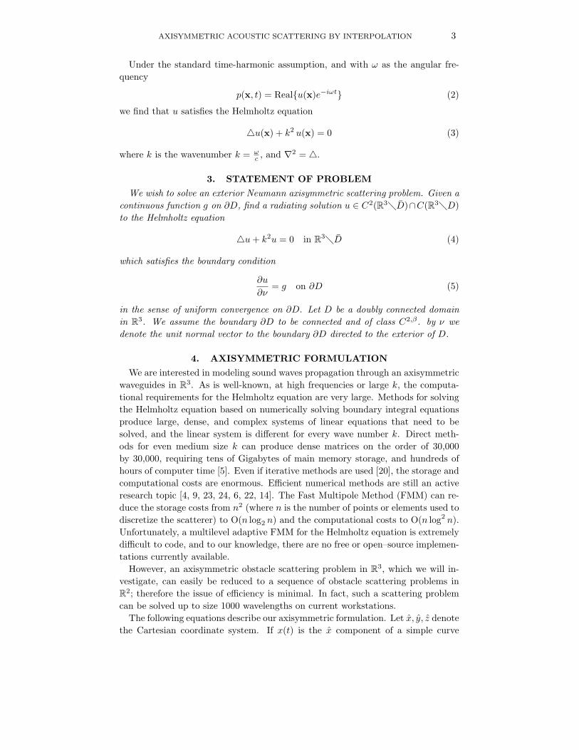
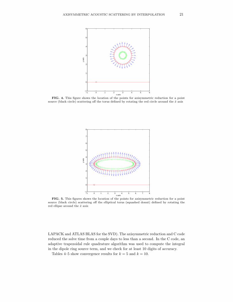
The last line in table 3 (labeled “Axisymmetric Reduction”) shows the resultsof implementing equation (87). The red circles in figure 4 show the location ofthe n secondary dipole ring sources {yj}, and the green circles show the locationof the m sampling locations {xi} on Γ. The black circle shows the location ofthe point source creating the incident field u0. The entire scattering algorithmwas implemented in 81 lines of matlab code. After verifying the results versus thefull R3 version, the algorithm was reimplemented in ANSI C (and as before, using
AXISYMMETRIC ACOUSTIC SCATTERING BY INTERPOLATION 21
−1 0 1 2 3 4 5 6−1
0
1
2
3
4
5
6
x axis
y ax
is
FIG. 4. This figure shows the location of the points for axisymmetric reduction for a pointsource (black circle) scattering off the torus defined by rotating the red circle around the x axis
−1 0 1 2 3 4 5 6 7 8−1
0
1
2
3
4
5
6
7
8
x axis
y ax
is
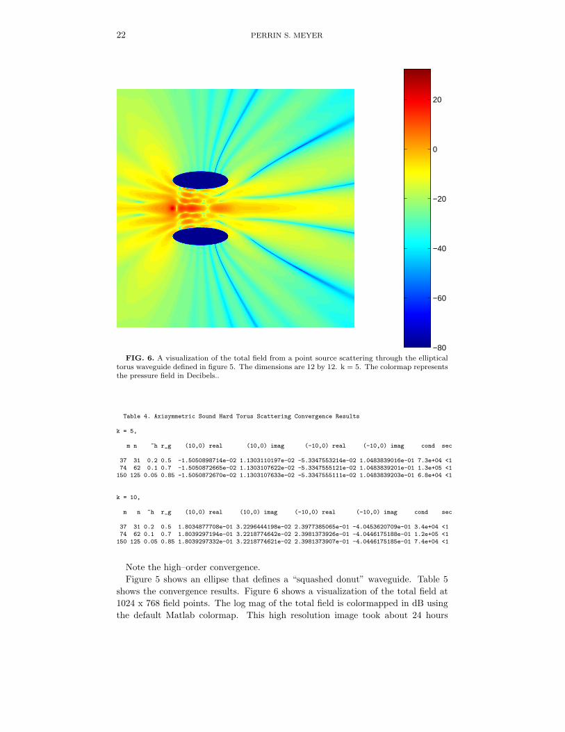
FIG. 5. This figures shows the location of the points for axisymmetric reduction for a pointsource (black circle) scattering off the elliptical torus (squashed donut) defined by rotating thered ellipse around the x axis
LAPACK and ATLAS BLAS for the SVD). The axisymmetric reduction and C codereduced the solve time from a couple days to less than a second. In the C code, anadaptive trapezoidal rule quadrature algorithm was used to compute the integralin the dipole ring source term, and we check for at least 10 digits of accuracy.
Tables 4–5 show convergence results for k = 5 and k = 10.
22 PERRIN S. MEYER
−80
−60
−40
−20
0
20
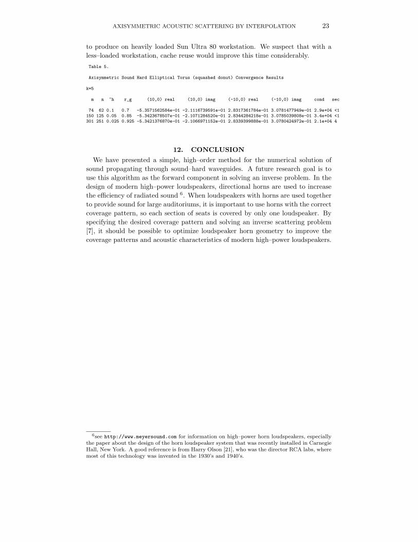
FIG. 6. A visualization of the total field from a point source scattering through the ellipticaltorus waveguide defined in figure 5. The dimensions are 12 by 12. k = 5. The colormap representsthe pressure field in Decibels..
Table 4. Axisymmetric Sound Hard Torus Scattering Convergence Results
k = 5,
m n ~h r_g (10,0) real (10,0) imag (-10,0) real (-10,0) imag cond sec
Note the high–order convergence.Figure 5 shows an ellipse that defines a “squashed donut” waveguide. Table 5
shows the convergence results. Figure 6 shows a visualization of the total field at1024 x 768 field points. The log mag of the total field is colormapped in dB usingthe default Matlab colormap. This high resolution image took about 24 hours
AXISYMMETRIC ACOUSTIC SCATTERING BY INTERPOLATION 23
to produce on heavily loaded Sun Ultra 80 workstation. We suspect that with aless–loaded workstation, cache reuse would improve this time considerably.Table 5.
Axisymmetric Sound Hard Elliptical Torus (squashed donut) Convergence Results
k=5
m n ~h r_g (10,0) real (10,0) imag (-10,0) real (-10,0) imag cond sec
12. CONCLUSIONWe have presented a simple, high–order method for the numerical solution of
sound propagating through sound–hard waveguides. A future research goal is touse this algorithm as the forward component in solving an inverse problem. In thedesign of modern high–power loudspeakers, directional horns are used to increasethe efficiency of radiated sound 6. When loudspeakers with horns are used togetherto provide sound for large auditoriums, it is important to use horns with the correctcoverage pattern, so each section of seats is covered by only one loudspeaker. Byspecifying the desired coverage pattern and solving an inverse scattering problem[7], it should be possible to optimize loudspeaker horn geometry to improve thecoverage patterns and acoustic characteristics of modern high–power loudspeakers.
6see http://www.meyersound.com for information on high–power horn loudspeakers, especiallythe paper about the design of the horn loudspeaker system that was recently installed in CarnegieHall, New York. A good reference is from Harry Olson [21], who was the director RCA labs, wheremost of this technology was invented in the 1930’s and 1940’s.
24 PERRIN S. MEYER
REFERENCES
1. Milton Abramowitz and Irene A. Stegun, editors. Handbook of Mathematical Functions WithFormulas, Graphs, and Mathematical Tables. Dover, New York, N.Y., 1972.
2. E. Anderson, Z. Bai, C. Bischof, S. Blackford, J. Demmel, J. Dongarra, J. Du Croz, A. Green-baum, S. Hammarling, A. McKenney, and D. Sorensen, editors. LAPACK Users Guide (ThirdEdition). Society for Industrial and Applied Mathematics (SIAM), Philedelphia, PA, 2000.http://www.netlib.org/lapack.
3. J. J. Bowman, T.B.A Senior, and P.L.E. Uslenghi, editors. Electromagnetic and AcousticScattering by Simple Shapes. North Holland, Amsterdam, 1969.
4. Oscar P. Bruno and Leonid A. Kunyansky. Fast, high-order solution of surface scatteringproblems. In Alfredo Bermudez et al., editor, Fith International Conference on Mathematicaland Numerial Aspects of Wave Propagation, pages 465–470. Society for Industrial and AppliedMathematics, 2000.
5. Lawrence F. Canino, John J. Ottusch, Mark A. Stalzer, John L. Visher, and Stephan M.Wandzura. Numerical solution of the Helmholtz equation in 2d and 3d using a high–orderNystrom discretization. Journal of Computational Physics, 146:627–663, 1998.
6. YH Chen, WC Chew, and S Zeroug. Fast multipole method as an efficient solver for 2d elasticwave surface integral equations. Computational Mechanics, 20(6):485–506, 1997.
8. Yu Chen and Sang-Yeun Shim. Solution of obstacle scattering problems by interpolation.Presented 9 October 2000 at The Courant Institute Numerical Analysis Seminar, (manuscriptin preparation).
9. H Cheng, L. Greengard, and V. Rokhlin. A fast adaptive multipole algorithm in three dimen-sions. Journal of Computational Physics, 155:468–498, 1999.
10. David Colton and Rainer Kress. Inverse Acoustic and Electromagnetic Scattering Theory,Second Edition. Springer–Verlag, Berlin, 1998.
11. Adrian Doicu, Yuri Eremin, and Thomas Wriedt. Acoustic and Electromagnetic ScatteringAnalysis Using Discrete Sources. Academic Press, San Diego, CA, 2000.
12. I.S. Gradshteyn, I.M Ryzhik, and Alan Jeffrey, editors. Table of Integrals, Series, and Prod-ucts. Academic Press, San Deigo, CA., fifth edition, 1994.
13. James J. Grannell, Joseph J. Shirron, and Luise S. Couchman. A hierarchic p-versionboundary–element method for axisymmetric acoustic scattering and radiation. Journal ofthe Acoustical Society of America, 95(5):2320–2329, 1994.
14. JS Jhao and WC Chew. Three-dimensional multilevel fast multipole algorithm from static toelectrodynamic. MICROW OPT TECHN LET, 26(1):43–48, 2000.
15. Rainer Kress. On constant alpha force–free fields. Journal of Engineering Math, 20:323–344,1986.
16. Rainer Kress. On the numerical solution of a hypersingular integral equation in scatteringtheory. Journal of Computational and Applied Mathematics, 61:345–360, 1995.
17. N.N. Lebedev. Special Functions and Their Applications. Dover, New York, 1972.
18. Gregory Matviyenko. On the azimuthal Fourier components of the Green’s function for theHelmholtz equation in three dimensions. Journal of Mathematical Physics, 36(9):5159–5169,1995.
19. Philip M. Morse and K. Uno Ingard. Theoretical Acoustics. Princeton University, Princeton,NJ, 1986.
20. Ramesh Natarajan. An iterative scheme for dense, complex-symetric, linear systems in acous-tics boundary-element computations. SIAM Journal on Scientific Computing, 19(5):1450–1470, 1998.
21. Harry F. Olson. Acoustical Engineering. D. Van Nostrand Company, Princeton, N.J., 1957.
22. JM Song, CC Lu, and WC Chew. Fast Illinois solver code (FISC). IEEE ANTENNASPROPAG, 40(3):27–35, 1998.
23. W. W. Symes. Cell–centered finite difference modeling for the 3-d Helmholtz problem. Tech-nical report, Rice University, 1996.
24. W. W. Symes. Iterative procedures for wave propagation in the frequency domain. Technicalreport, Rice University, 1996.


![New Iterative Methods for Interpolation, Numerical ... · and Aitken’s iterated interpolation formulas[11,12] are the most popular interpolation formulas for polynomial interpolation](https://static.documents.pub/doc/80x56/5ebfad147f604608c01bd287/new-iterative-methods-for-interpolation-numerical-and-aitkenas-iterated-interpolation.jpg)


