Utah State University Utah State University DigitalCommons@USU DigitalCommons@USU All Graduate Theses and Dissertations Graduate Studies 12-2010 Axisymmetric Finite Element Modeling for the Design and Axisymmetric Finite Element Modeling for the Design and Analysis of Cylindrical Adhesive Joints based on Dimensional Analysis of Cylindrical Adhesive Joints based on Dimensional Stability Stability Paul E. Lyon Utah State University Follow this and additional works at: https://digitalcommons.usu.edu/etd Part of the Mechanical Engineering Commons Recommended Citation Recommended Citation Lyon, Paul E., "Axisymmetric Finite Element Modeling for the Design and Analysis of Cylindrical Adhesive Joints based on Dimensional Stability" (2010). All Graduate Theses and Dissertations. 784. https://digitalcommons.usu.edu/etd/784 This Thesis is brought to you for free and open access by the Graduate Studies at DigitalCommons@USU. It has been accepted for inclusion in All Graduate Theses and Dissertations by an authorized administrator of DigitalCommons@USU. For more information, please contact [email protected].
Transcript
Utah State University Utah State University
DigitalCommons@USU DigitalCommons@USU
All Graduate Theses and Dissertations Graduate Studies
12-2010
Axisymmetric Finite Element Modeling for the Design and Axisymmetric Finite Element Modeling for the Design and
Analysis of Cylindrical Adhesive Joints based on Dimensional Analysis of Cylindrical Adhesive Joints based on Dimensional
Stability Stability
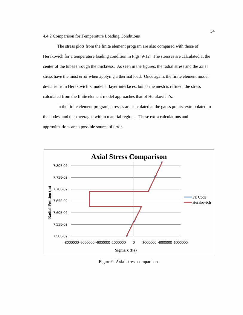
Paul E. Lyon Utah State University
Follow this and additional works at: https://digitalcommons.usu.edu/etd
Part of the Mechanical Engineering Commons
Recommended Citation Recommended Citation Lyon, Paul E., "Axisymmetric Finite Element Modeling for the Design and Analysis of Cylindrical Adhesive Joints based on Dimensional Stability" (2010). All Graduate Theses and Dissertations. 784. https://digitalcommons.usu.edu/etd/784
This Thesis is brought to you for free and open access by the Graduate Studies at DigitalCommons@USU. It has been accepted for inclusion in All Graduate Theses and Dissertations by an authorized administrator of DigitalCommons@USU. For more information, please contact [email protected].
Axisymmetric Finite Element Modeling for the Design and Analysis of
Cylindrical Adhesive Joints based on Dimensional Stability
by
Paul E. Lyon, Master of Science
Utah State University, 2010
Major Professor: Dr. Thomas H. Fronk Department: Mechanical and Aerospace Engineering The use and implementation of adhesive joints for space structures is necessary for
incorporating fiber-reinforced composite materials. Correct modeling and design of cylindrical
adhesive joints can increase the dimensional stability of space structures. The few analytical
models for cylindrical adhesive joints do not fully describe the displacement or stress field of the
joint.
A two-dimensional axisymmetric finite element model for the design and analysis of
adhesive joints was developed. The model was developed solely for the analysis of cylindrical
adhesive joints, but the energy techniques used to develop the model can be applied to other types
of joints as well. A numerical program was written to solve the system of equations [K]d=R
for the unknown displacements d. The displacements found from the program are used to
design cylindrical adhesive joints based on dimensional stability. Stresses were calculated from
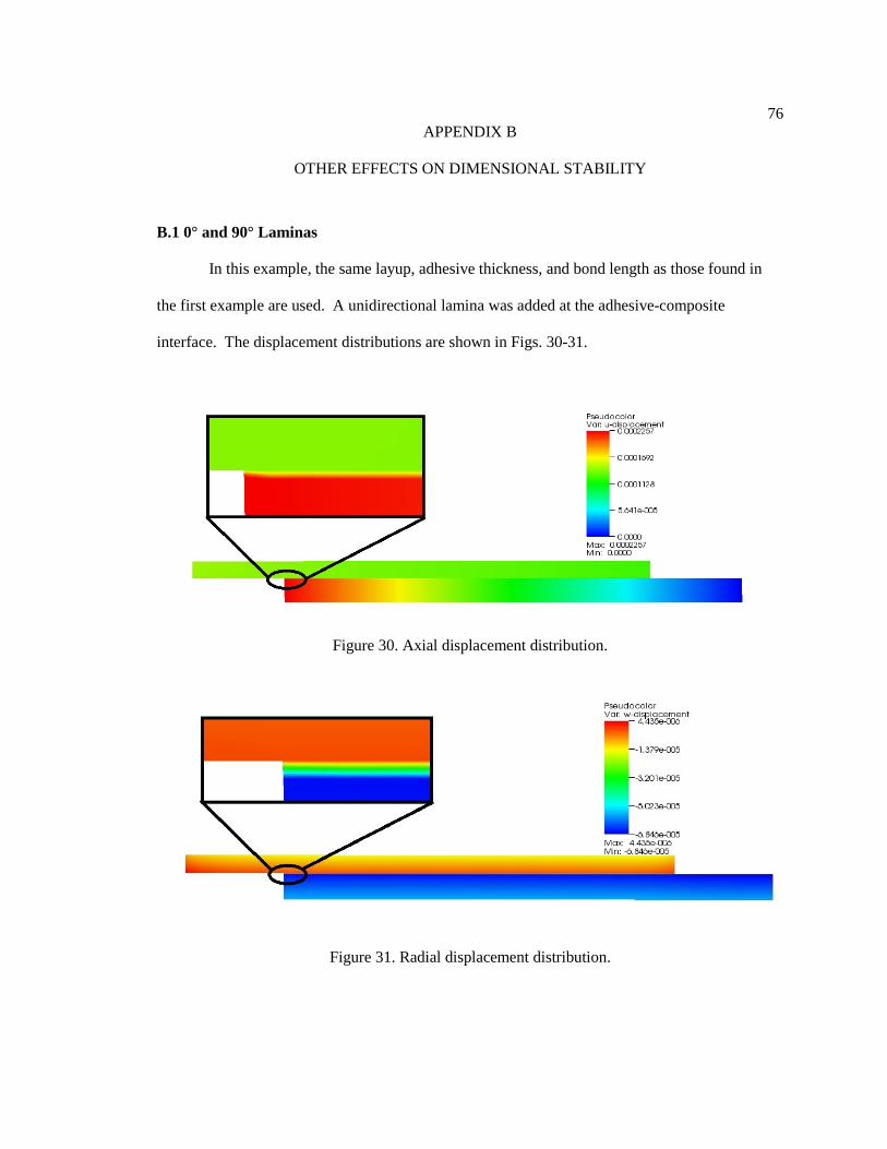
the displacements for comparison with analytical models. The cylindrical joints were assumed to
remain within the linear elastic region and no failure criteria was taken into account.
The design process for cylindrical joints was developed based on dimensional stability.
The nodal displacements found from the finite element model were used in the optimization of
iv
geometric parameters of cylindrical joints. The stacking sequence of the composite, the bond
length, and the bond thickness were found to have the greatest impact on dimensional stability.
Other factors that were found to further reduce the maximum displacements are the
implementation of 0° and 90° laminas, the isotropic cylinder thickness, tapering of the isotropic
cylinder, and the inside radius of the cylindrical joint.
This axisymmetric finite element model is beneficial in that a cylindrical joint can be
designed before any testing is performed. The results and cases in this thesis are generalized in
order to show how the design process works. The model can be used in conjunction with design
requirements for a specific joint to reduce the maximum displacements below any specified
operating requirements. The joint is dimensionally stable if the overall displacements meet
specific design requirements.
(273 pages)
v
ACKNOWLEDGMENTS
I would like to thank Dr. Thomas Fronk for all of his help, guidance, and encouragement
for me in my graduate studies. This thesis would not have been possible without his willingness
and exceptional ability to teach and help me understand the engineering concepts and theories I
have used in this research. I would also like to thank Michael Lambert for all of his help and
support in learning and applying the theory of joining dissimilar materials. The experience I have
gained from performing this research and working with Dr. Fronk and Michael Lambert is
exceptional.
I would like to thank the Space Dynamics Lab for funding this research and having
interest in this area of engineering. I hope that the contents of this thesis can benefit them in the
further design and development of their space structures. I would like to thank the members of
my committee, Dr. Steven Folkman and Dr. Leijun Li, for their suggestions and guidance.
Thanks Dr. Li for being willing to join my committee at such late notice.
I would especially like to thank my family for the support and encouragement in
obtaining my undergraduate and graduate educations. I would like to express sincere
appreciation to my wife, Kara Jo, for all of her patience and support in every aspect of my college
career.
Paul E. Lyon
vi
CONTENTS
Page ABSTRACT .................................................................................................................................... iii
ACKNOWLEDGMENTS ............................................................................................................... v
LIST OF TABLES ........................................................................................................................ viii
LIST OF FIGURES ........................................................................................................................ ix
6. Material Properties f(T) Explanation ..................................................................................... 39
ix
LIST OF FIGURES Figure Page 1. Gant chart for current research. ................................................................................................. 7
2. A typical cylindrical adhesive joint. ........................................................................................ 10
3. Axisymmetric Mesh Program.f95 program flowchart. ........................................................... 23
4. Fecode.f95 program flowchart. ............................................................................................... 26
The object of this thesis is to develop a two-dimensional axisymmetric finite element
model for the design and analysis of cylindrical adhesive joints. The finite element model is used
to design cylindrical adhesive joints based solely on dimensional stability requirements.
Although dimensional stability implies more than just deformations due to thermal loads, only
temperature effects are taken into account in this model. All materials used in the analyses
performed with this model are assumed to remain within the linear elastic region and no failure
criteria is taken into account.
Fiber-reinforced composite materials have become very beneficial in the application of
lightweight space structures. Not only are they useful because of their light weight and high
strength capabilities, but their coefficients of thermal expansion (CTE) are low compared to most
isotropic metals. These physical properties are also tailorable to the needs of the application.
Composite materials can help improve the dimensional stability of a structure because they can be
tailored to minimize deformations due to thermal loads.
Joining composite materials to isotropic materials for structural applications must be
done in a way that will not significantly reduce the strength of the composite. Some joining
techniques such as bolting or riveting can lead to delamination of the composite. The use of an
adhesive to join a composite material to an isotropic material can be done such that it does not
cause high stress concentration or reduction of strength in the composite. There are many
different types of joining techniques available. Cylindrical joining is advantageous due to the
simplicity of manufacturing composite cylinders and the ability to mount flight components or
hardware to the cylinders. In most cases, a cylindrical configuration can be considered an
axisymmetric problem.
2
Many different analytical solutions have been developed to analyze the stress field in an
adhesive joint. Adhesive joints create a complicated three-dimensional state of stress that cannot
be analyzed fully, or exactly, with a closed-form solution. Most of the analytical models
developed to date look at stresses but not displacements. In order to design adhesive joints based
on dimensional stability, displacements, instead of stresses, need to be taken into account and
minimized. The benefit of a finite element model specific to adhesive joints is that displacements
can be found directly at the nodes and interpolated within elements. The displacement field over
the entire joint can also be found with a finite element model.
The research for this thesis was performed for and funded by the Space Dynamics Lab
(SDL) in Logan, UT, in fulfillment of a research contract. Although the research was performed
specifically for SDL, the content found in this thesis can be utilized and applied to any cylindrical
adhesive joint design. Practicing engineers working with fiber-reinforced composite materials
can greatly benefit by utilizing the design techniques described herein.
The main body of this thesis contains the development of a two-dimensional
axisymmetric finite element model. It also contains an extensive literature review, model
verification, a cylindrical joint design procedure, and a summary of the results of the research and
work performed.
3
CHAPTER 2
LITERATURE REVIEW 2.1 Introduction
The literature review presented in this chapter covers different analysis techniques for
adhesive joints and the effects of composite stacking sequence, bond thickness, and bond length
on joint strength and dimensional stability. A more general literature review on adhesive joints is
presented in Appendix A.
2.2 Analysis Techniques
For over seventy years, analysis techniques have been researched for adhesive joints.
Most of these analyses have been developed to predict the stress field in a joint. Two of the most
basic models were developed by Volkersen [1] in 1938 and Goland and Reissner [2] in 1944.
Both of these models were based off of a plane stress assumption. Volkersen did not take into
account the thickness of the adhesive and assumed that all deformation was axial. Goland et al.
took into account the bending moment induced by the eccentric loading of a single lap joint.
Hart-Smith [3-6] performed different analyses on standard adhesive joints and more complex
adhesive joints found in the aerospace industry. He took into account the out-of-plane stresses
and included anisotropic material properties for the adherends. The adherends in his analyses
could be similar or dissimilar. In 1989, Crocombe and Bigwood [7] took into account the out-of-
plane normal (peel) and shear stresses. These stresses were found to be very important due to the
eccentric axial loading conditions of a single lap adhesive joint. In 1975, Renton and Vinson [8]
accurately portrayed the stress distributions in the adhesive and the adherends. He also
contributed to the adhesive joining of fiber-reinforced materials [9].
An analysis applicable to joining cylindrical tubes was developed by Nemes et al. [10] in
2007 and Shi and Cheng [11] in 1993. They both performed analyses on cylindrical adhesive
4
joints and developed the circumferential and shear stress distributions along the length of the
adhesive.
All of these models discussed so far are analytical models with some kind of underlying
assumptions. It is difficult to describe the three-dimensional state of stress experienced by an
adhesive joint with an analytical solution. To accurately describe the three-dimensional stress
distribution in the joint, some kind of numerical model is needed. Various finite element models
have been developed and incorporated for specific purposes. Bartoszyk et al. [12] in their design
of the truss structure for the James Webb Space Telescope (JWST) in 1990 developed a finite
element model to predict the structure’s dimensional stability. They developed a three-
dimensional model to design their adhesive joints based on a stress-based failure theory.
The dimensional stability of the JWST has been a key issue studied by Cifie et al. [13].
In order to improve the focusing capabilities of the telescope, they developed a finite element
model to determine the behavior of the support structure under thermal loads. They found that
the dimensional stability of the composite laminate in the joint is dominated by the smeared hoop
CTE, which should be zero or slightly negative.
2.3 Composite Stacking Sequence
The stacking sequence of the composite was researched by Bartoszyk et al. [12] in their
work on the JWST. They applied a unidirectional inner lamina on the composite-adhesive
interface of the joint to sustain the transverse shear and normal stresses. They also used it to
decrease the CTE mismatch between the composite and the adhesive. This inner lamina
consisted of different fibers than the rest of the composite.
2.4 Bond Thickness
Overall, a thinner bondline thickness was observed to increase the joint strength. For his
tests in 1974, Hart-Smith [5] proposed an optimum bondline thickness of 0.1 mm to 0.15 mm.
5
While performing tests in 1982, Hylands [14] observed that the use of thin adhesive bonds
resulted in stronger joints.
Anderson et al. [15] in 1982 found that decreasing the bondline thickness resulted in a
more uniform stress distribution. In their research on adhesive properties at cryogenic
temperatures in 1982, Shimoda et al. [16] showed that the adhesive bond strength is sensitive to
the bondline thickness.
2.5 Bond Length
From his literature review in 2004, Baldan [17] stated that the shear stresses being
uniformly distributed along the length of the bond, or overlap length, is an incorrect assumption.
He stated that doubling the overlap length will not double the load capacity. Although most
overlap lengths are determined by empirical results of lap shear tests, Hart-Smith [3], in 1973,
established an equation to optimize the overlap length for maximum joint strength of a single lap
joint. He also pointed out that there is a critical overlap length required to fully transfer the load
across the joint, and any extra length becomes redundant. Renton and Vinson [18], in 1975, made
a similar conclusion; redundant overlap length diminishes the positive stress returns. In
conjunction with Hart-Smith and Renton and Vinson, Kim et al. [19], in 2008, found the overlap
length to be effective only within a limited range. He concluded that with an overlap length-to-
width ratio less than one, the failure load increases as overlap length decreases, with an overlap
length-to-width ratio greater than one the failure load only increases slightly.
In 2001, Potter et al. [20] also recognized that the overlap length is critical to joint
strength. They found that it needs to be long enough to transfer the applied load across the joint
without experiencing failure in the middle of the joint. They also observed that the overlap length
affects the crack propagation distance in the adhesive before reaching a critical crack length. In
their testing of composite joints for cryogenic applications in 2007, Graf et al. [21] found an
optimized overlap length of 7.62 cm for their test specimens.
6
CHAPTER 3
OBJECTIVES The purposes of this research are to gain a general knowledge and understanding of
cylindrical adhesive joints, model their behavior due to thermal loads, and optimize their
dimensions based on dimensional stability. These purposes will be accomplished by performing
the following tasks.
• Perform an extensive literature review to increase the general understanding and knowledge of adhesive joints.
• Derive mathematical expressions for a two-dimensional axisymmetric finite element
model in cylindrical coordinates.
• Write a numerical program in FORTRAN for the finite element model.
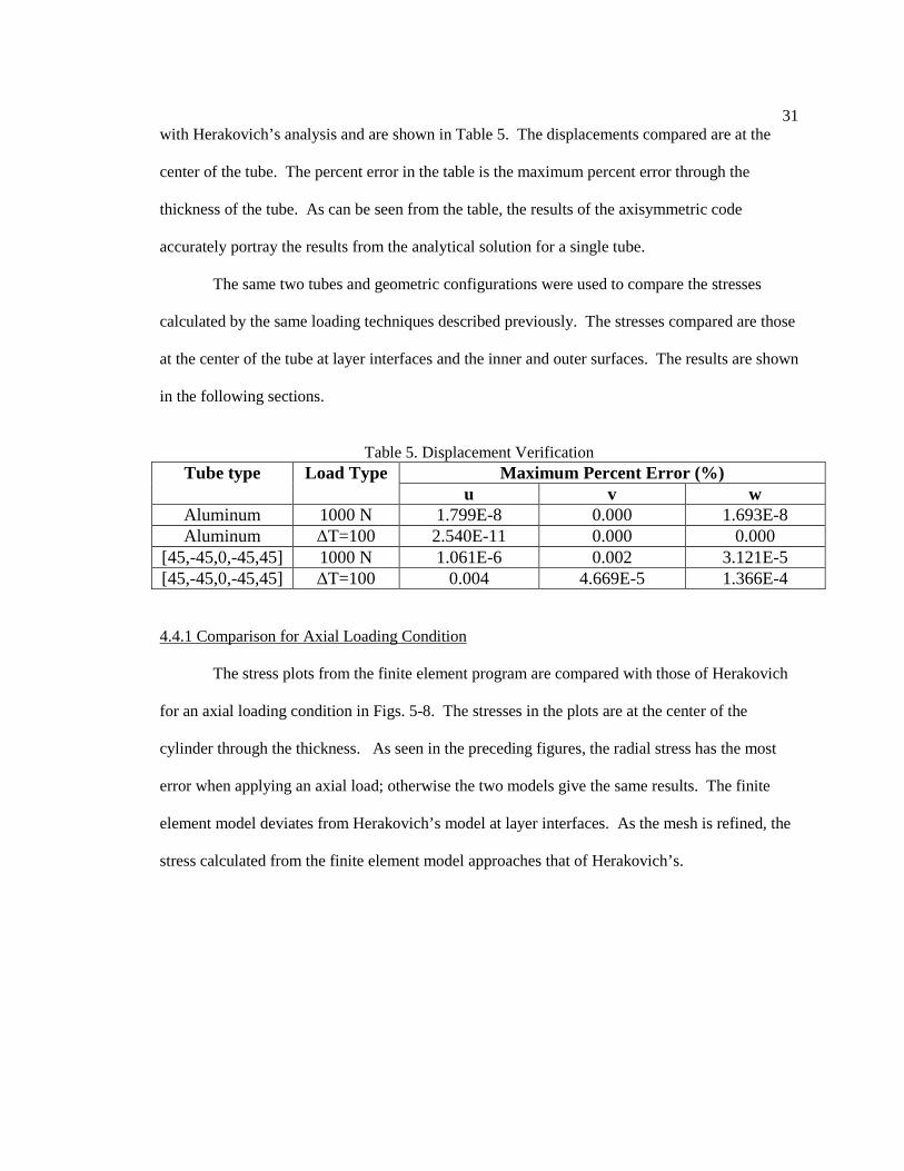
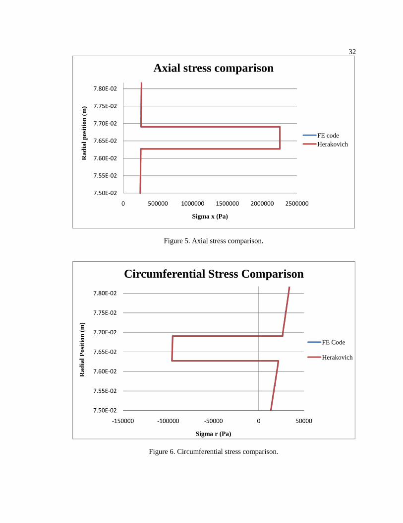
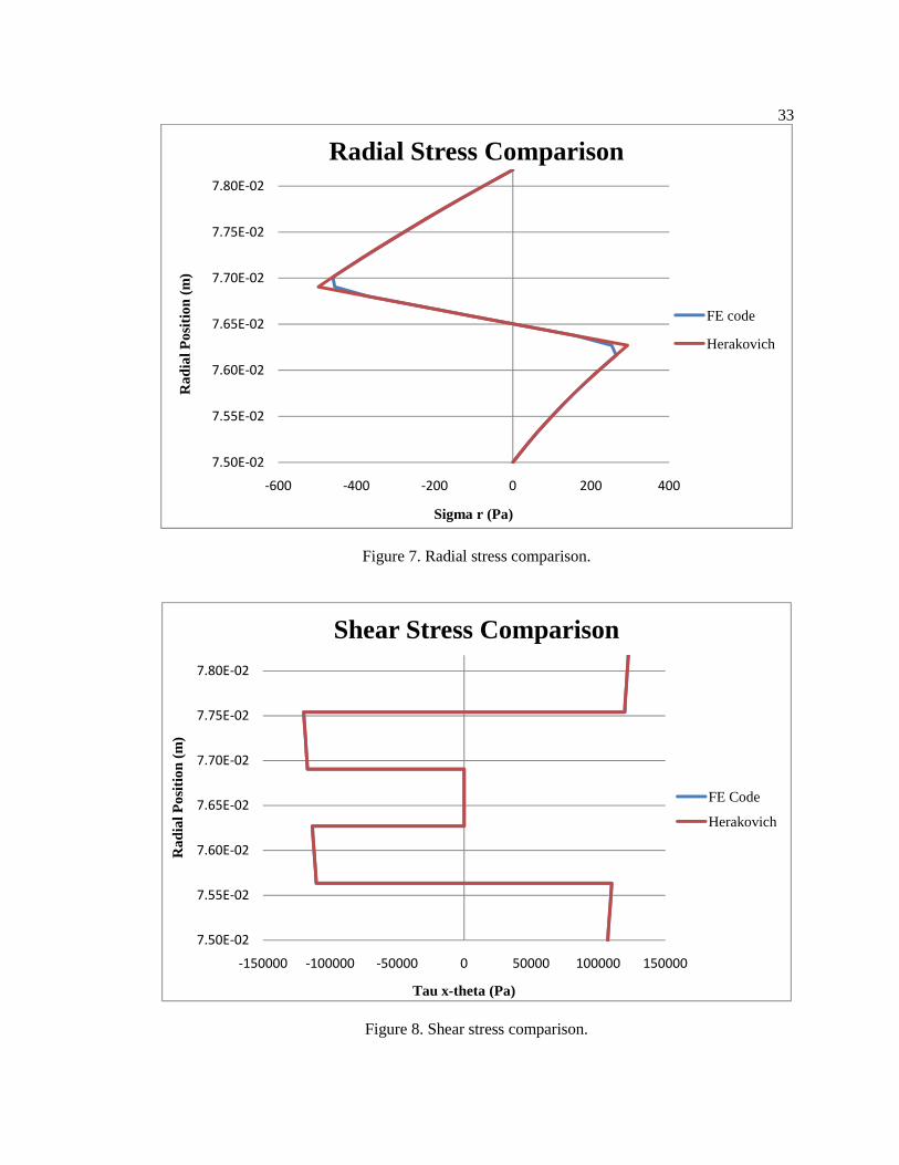
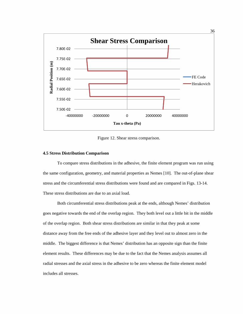
• Verify the results of the finite element model by comparing displacements and stresses of a single cylinder with Herakovich’s analytical model.
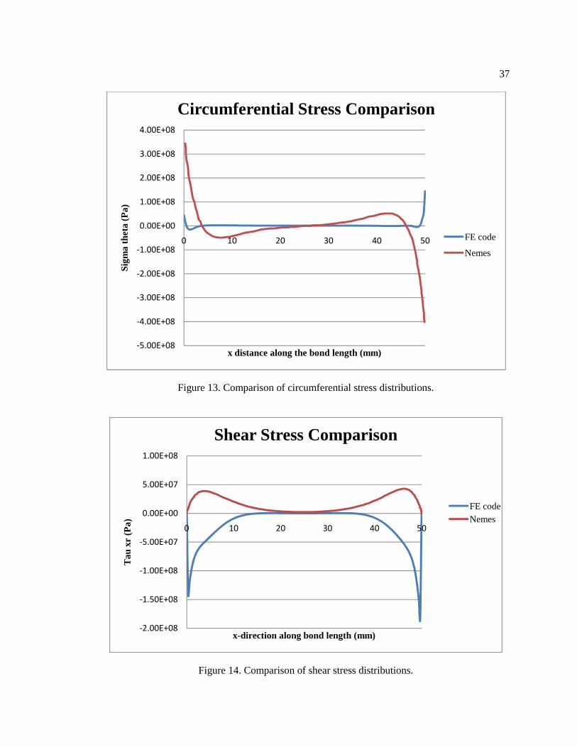
• Compare the stress distribution through the adhesive layer of a cylindrical adhesive joint
with the model developed by Nemes.
• Incorporate material properties as a function of temperature into the finite element model.
• Use the model to minimize deformations of cylindrical adhesive joints by optimizing the bond length and thickness and the stacking sequence of the composite laminate.
• Summarize the results of this research and recommend future work.
7
CHAPTER 4
APPROACH
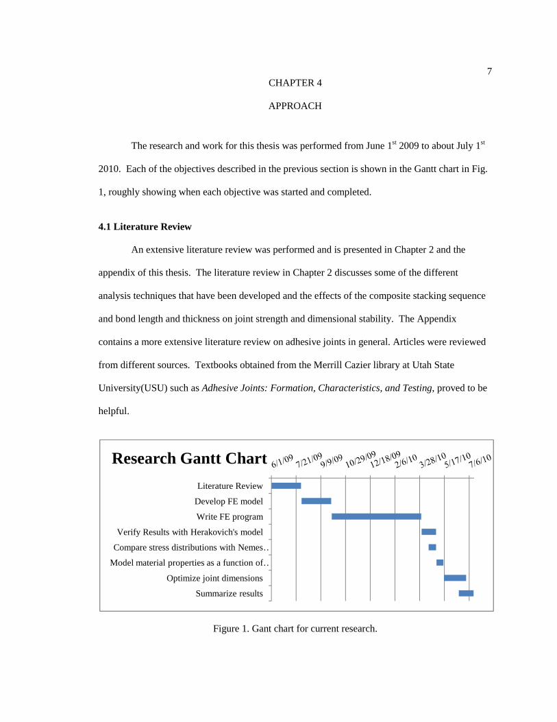
The research and work for this thesis was performed from June 1st 2009 to about July 1st
2010. Each of the objectives described in the previous section is shown in the Gantt chart in Fig.
1, roughly showing when each objective was started and completed.
4.1 Literature Review
An extensive literature review was performed and is presented in Chapter 2 and the
appendix of this thesis. The literature review in Chapter 2 discusses some of the different
analysis techniques that have been developed and the effects of the composite stacking sequence
and bond length and thickness on joint strength and dimensional stability. The Appendix
contains a more extensive literature review on adhesive joints in general. Articles were reviewed
from different sources. Textbooks obtained from the Merrill Cazier library at Utah State
University(USU) such as Adhesive Joints: Formation, Characteristics, and Testing, proved to be
helpful.
Figure 1. Gant chart for current research.
Literature Review
Develop FE model
Write FE program
Verify Results with Herakovich's model
Compare stress distributions with Nemes …
Model material properties as a function of …
Optimize joint dimensions
Summarize results
Research Gantt Chart
8
Online sources including EBSCO host, Scirus, Worldcat, and the electronic journals list from the
library provided many useful articles. The most helpful source was the NASA Technical Reports
Server (NTRS). This server contains technical articles on research contracted by NASA that have
been performed by various organizations and people.
For each article found, a summary was written of the main points that were relevant to
the design and application of adhesive joints. The summaries of each article were then compiled
into different categories and the literature review was written. A bibliography was recorded in
order to cite each of the articles.
4.2 Finite Element Model Development
Many previous mathematical models were compiled and reviewed during the literature
review. Some of the most important models included the Hart-Smith [3,5] single-lap and double-
lap joint models, the Renton and Vinson [18] model utilizing composite adherends, and the Shi
[11] and Nemes [10] models for cylindrical configurations. These analytical models have some
kind of simplifying assumptions and do not fully model the three-dimensional state of stress near
the free edges of the overlap region. These stresses within the overlap region are critical because
they can cause delamination and ultimately failure within the composite cylinder.
After performing the literature review, several attempts were made to develop simplified
mathematical models based on plate or thin shell theory to accurately represent a cylindrical
adhesive joint. These simplified theories cannot accurately predict the state of stress near the free
edges of the overlap region of the joint as a three-dimensional model will.
For predicting dimensional stability, the only load that is applied in order to optimize the
joint geometry is a constant temperature load. Since this thermal loading is uniform throughout
the joint and the geometry of the joint is cylindrical, the three-dimensional analysis can be
simplified to an axisymmetric analysis. This allows for the use of planar elements instead of
solid elements in the finite element model.
9
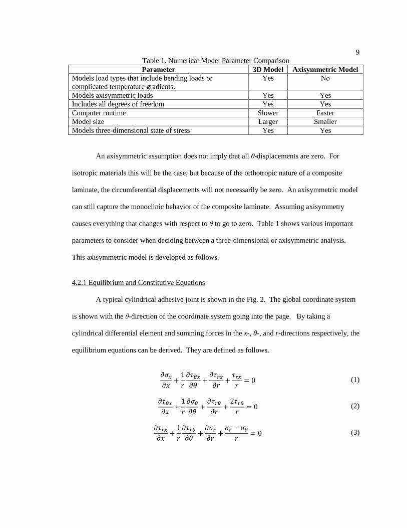
Table 1. Numerical Model Parameter Comparison Parameter 3D Model Axisymmetric Model
Models load types that include bending loads or complicated temperature gradients.
Yes No
Models axisymmetric loads Yes Yes Includes all degrees of freedom Yes Yes Computer runtime Slower Faster Model size Larger Smaller Models three-dimensional state of stress Yes Yes
An axisymmetric assumption does not imply that all θ-displacements are zero. For
isotropic materials this will be the case, but because of the orthotropic nature of a composite
laminate, the circumferential displacements will not necessarily be zero. An axisymmetric model
can still capture the monoclinic behavior of the composite laminate. Assuming axisymmetry
causes everything that changes with respect to θ to go to zero. Table 1 shows various important
parameters to consider when deciding between a three-dimensional or axisymmetric analysis.
This axisymmetric model is developed as follows.
4.2.1 Equilibrium and Constitutive Equations
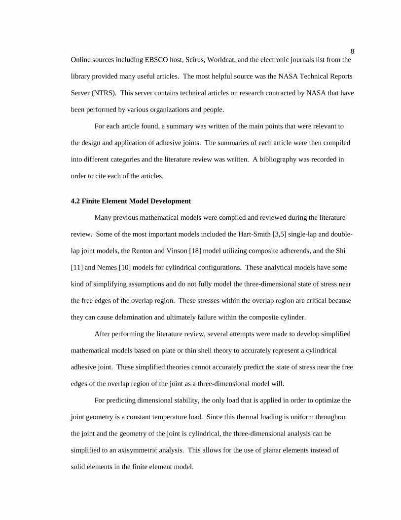
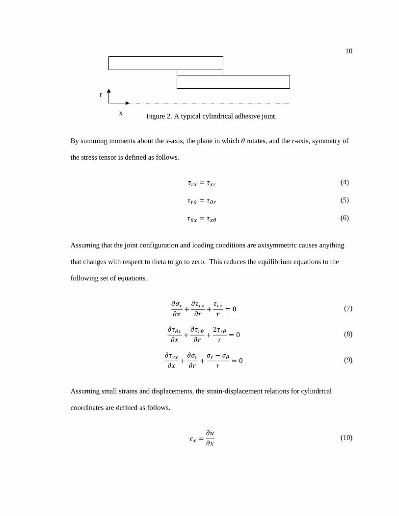
A typical cylindrical adhesive joint is shown in the Fig. 2. The global coordinate system
is shown with the θ-direction of the coordinate system going into the page. By taking a
cylindrical differential element and summing forces in the x-, θ-, and r-directions respectively, the
equilibrium equations can be derived. They are defined as follows.
1 0 (1)
1 2 0 (2)
1 0 (3)
10
Figure 2. A typical cylindrical adhesive joint.
By summing moments about the x-axis, the plane in which θ rotates, and the r-axis, symmetry of
the stress tensor is defined as follows.
(4) (5) (6) Assuming that the joint configuration and loading conditions are axisymmetric causes anything
that changes with respect to theta to go to zero. This reduces the equilibrium equations to the
following set of equations.
0 (7)
2 0 (8)
0 (9)
Assuming small strains and displacements, the strain-displacement relations for cylindrical
coordinates are defined as follows.
(10)
x
r
11
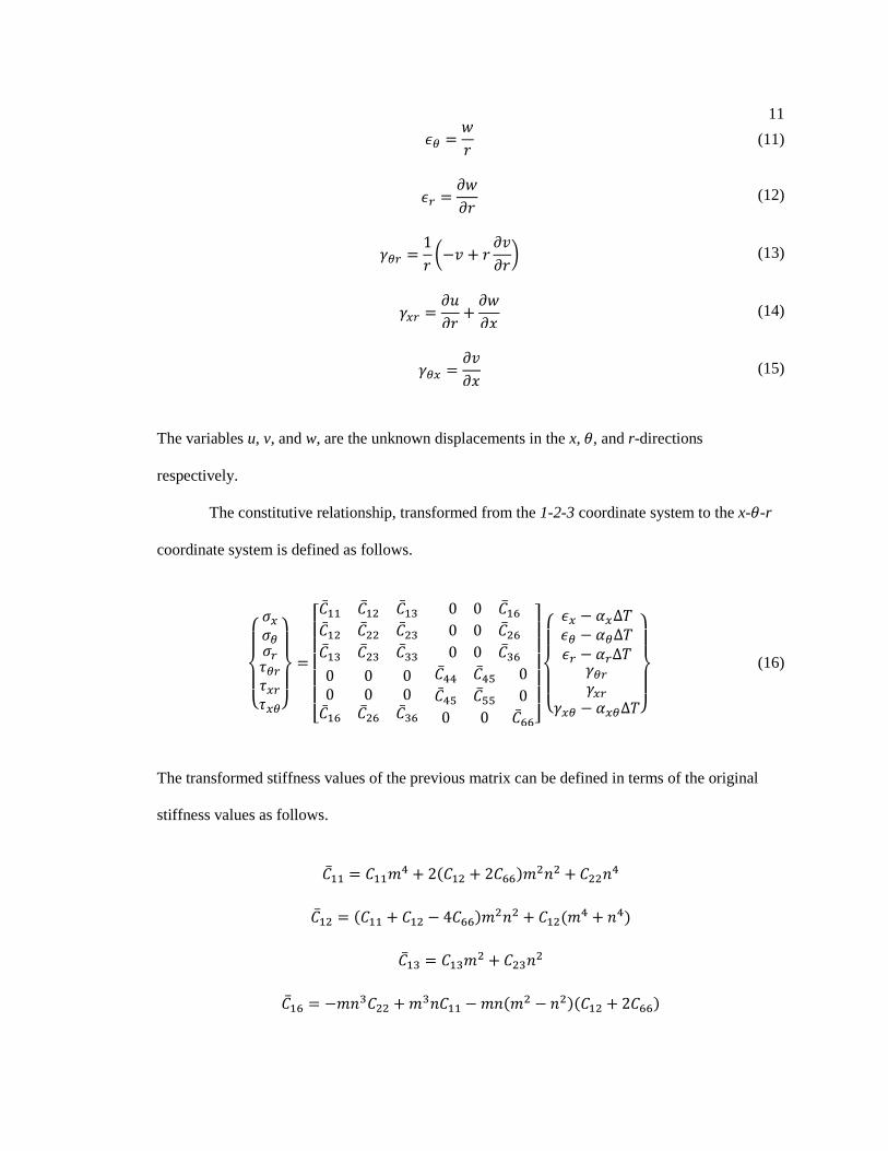
(11)
(12)
1 (13)
(14)
(15)
The variables u, v, and w, are the unknown displacements in the x, , and r-directions
respectively.
The constitutive relationship, transformed from the 1-2-3 coordinate system to the x--r
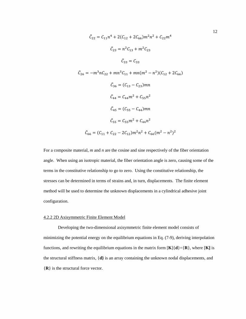
"#%% "$$3( 21"$% 2"''20%3% "%%0( "#%& 3%"$& 0%"%& "#&& "&& "#%' 0&3"%% 03&"$$ 0310% 3%21"$% 2"''2 "#&' 1"$& "%&203 "#(( "((0% "))3% "#() 1")) "((203 "#)) "))0% "((3% "#'' 1"$$ "%% 2"$%20%3% "''10% 3%2% For a composite material, m and n are the cosine and sine respectively of the fiber orientation
angle. When using an isotropic material, the fiber orientation angle is zero, causing some of the
terms in the constitutive relationship to go to zero. Using the constitutive relationship, the
stresses can be determined in terms of strains and, in turn, displacements. The finite element
method will be used to determine the unknown displacements in a cylindrical adhesive joint
configuration.
4.2.2 2D Axisymmetric Finite Element Model
Developing the two-dimensional axisymmetric finite element model consists of
minimizing the potential energy on the equilibrium equations in Eq. (7-9), deriving interpolation
functions, and rewriting the equilibrium equations in the matrix form [K ] d= R, where [K] is
the structural stiffness matrix, d is an array containing the unknown nodal displacements, and
R is the structural force vector.
13
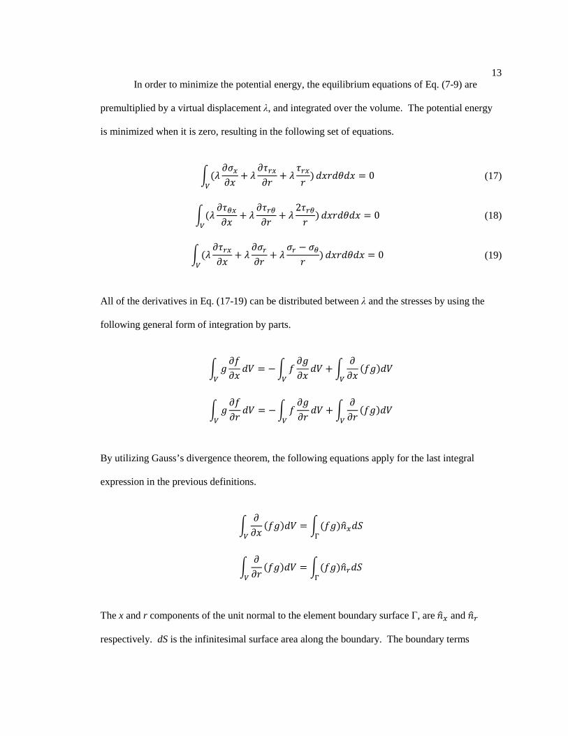
In order to minimize the potential energy, the equilibrium equations of Eq. (7-9) are
premultiplied by a virtual displacement λ, and integrated over the volume. The potential energy
is minimized when it is zero, resulting in the following set of equations.
5 16 6 6 2 7 888 0 (17)
5 16 6 6 2 2 7 888 0 (18)
5 16 6 6 2 7 888 0 (19)
All of the derivatives in Eq. (17-19) can be distributed between λ and the stresses by using the
following general form of integration by parts.
5 9 : 7 8; 5 : 9 8;
7 5 7 1:928;
5 9 : 7 8; 5 : 9 8;
7 5 7 1:928;
By utilizing Gauss’s divergence theorem, the following equations apply for the last integral
expression in the previous definitions.
5 7 1:928; 5 1:923<8=
>
5 7 1:928; 5 1:923<8=
>
The x and r components of the unit normal to the element boundary surface Γ, are 3< and 3<
respectively. dS is the infinitesimal surface area along the boundary. The boundary terms
14
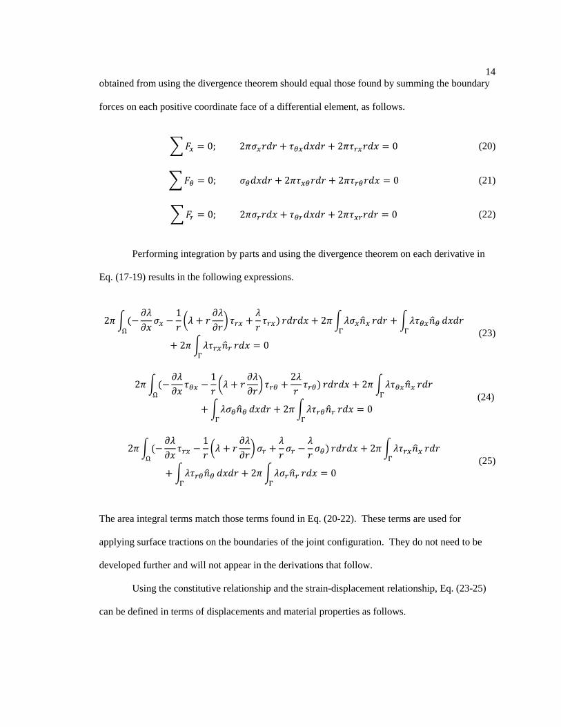
obtained from using the divergence theorem should equal those found by summing the boundary
forces on each positive coordinate face of a differential element, as follows.
? @ 0; 2B8 88 2B8 0 (20)
? @ 0; 88 2B8 2B8 0 (21)
? @ 0; 2B8 88 2B8 0 (22)
Performing integration by parts and using the divergence theorem on each derivative in
Eq. (17-19) results in the following expressions.
2B 5 1 6 1 6 6 6 2 Ω 88 2B 5 63<
> 8 5 63< > 88
2B 5 63< > 8 0
(23)
2B 5 1 6 1 6 6 26 2 Ω 88 2B 5 63<
> 8 5 63<
> 88 2B 5 63< > 8 0
(24)
2B 5 1 6 1 6 6 6 6 2 Ω 88 2B 5 63<
> 8 5 63<
> 88 2B 5 63< > 8 0
(25)
The area integral terms match those terms found in Eq. (20-22). These terms are used for
applying surface tractions on the boundaries of the joint configuration. They do not need to be
developed further and will not appear in the derivations that follow.
Using the constitutive relationship and the strain-displacement relationship, Eq. (23-25)
can be defined in terms of displacements and material properties as follows.
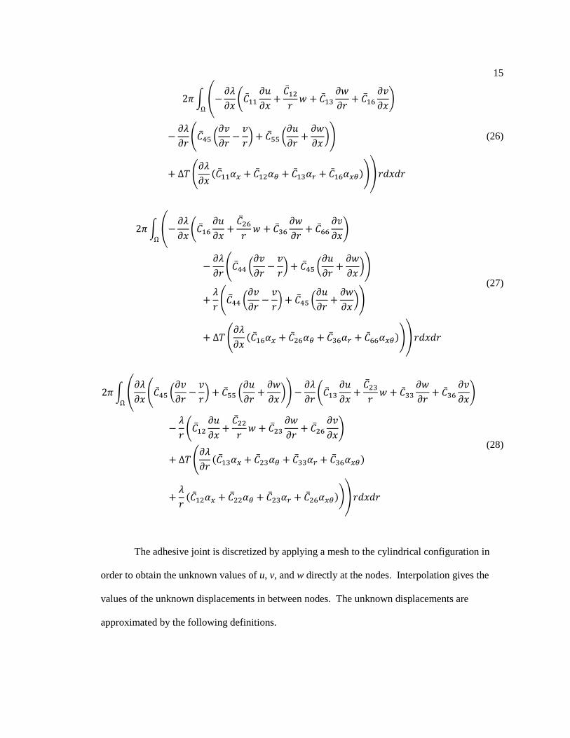
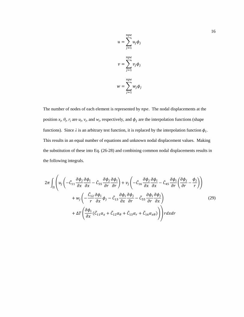
The adhesive joint is discretized by applying a mesh to the cylindrical configuration in
order to obtain the unknown values of u, v, and w directly at the nodes. Interpolation gives the
values of the unknown displacements in between nodes. The unknown displacements are
approximated by the following definitions.
16
? KLKMNOKP$
? KLKMNOKP$
? KLKMNOKP$
The number of nodes of each element is represented by 3QR. The nodal displacements at the
position xj, θj, rj are uj, vj, and wj, respectively, and LK are the interpolation functions (shape
functions). Since λ is an arbitrary test function, it is replaced by the interpolation function LS. This results in an equal number of equations and unknown nodal displacement values. Making
the substitution of these into Eq. (26-28) and combining common nodal displacements results in
the following integrals.
2B 5 DK E"#$$ LK LS "#)) LK LS F K G"#$' LK LS "#() LS ELK LK FH Ω
K E "#$% LS LK "#$& LS LK "#)) LS LK F ∆/ GLS 1"#$$- "#$%- "#$&- "#$'-2HJ 88
(29)
17
2B 5 DK G"#$' LS LK "#() ELK LS LS LK FH Ω
K G"#'' LS LK "#(( ELS LK LS LK LK LS LKLS% FH K E "#%' LS LK "#&' LS LK "#() LS LK "#() LK LSF ∆/ GLS 1"#$'- "#%'- "#&'- "#''-2HJ 88
(30)
2B 5 DK E"#)) LS LK "#$& LS LK "#$% LK LSF Ω
K E"#() LS ELK LK F "#&' LS LK "#%' LK LSF K E"#)) LS LK "#%& ELS LK LK LS F "#&& LK LS "#%%% LSLKF ∆/ GLS 1"#$&- "#%&- "#&&- "#&'-2 LS 1"#$%- "#%%- "#%&- "#%'-2FJ 88
(31)
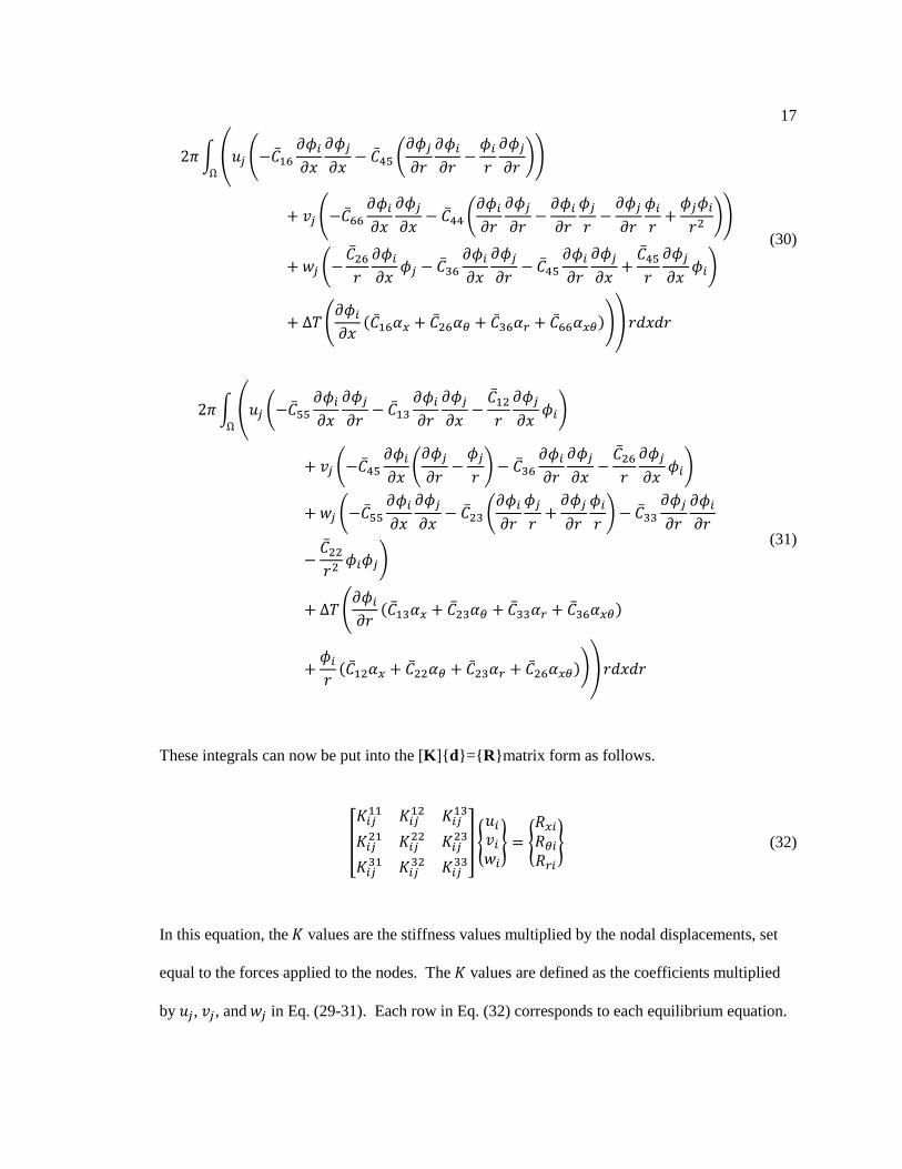
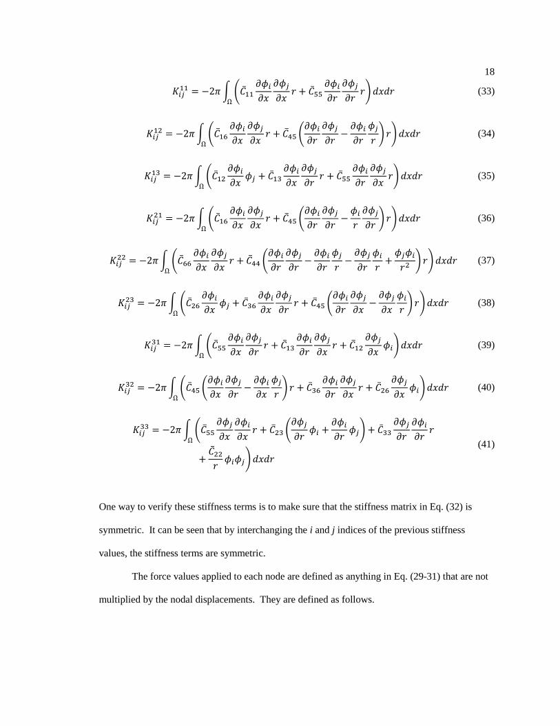
These integrals can now be put into the [K ] d= Rmatrix form as follows.
The shape functions are defined in Cook et al. [22] and are repeated here for
convenience. The node numbering for the following elements follows the standard node
numbering scheme for four-node and eight-node elements. The variables Z and [ are the local
coordinates of each individual element. For a linear four-node planar element, the shape
functions are defined as follows.
L$ 14 11 Z211 [2 (45)
L% 14 11 Z211 [2 (46)
L& 14 11 Z211 [2 (47)
L( 14 11 Z211 [2 (48)
For a quadratic eight-node planar element, the shape functions are defined as follows.
L$ 14 11 Z211 [2 12 1L\ L)2 (49)
L% 14 11 Z211 [2 12 1L) L'2 (50)
20
L& 14 11 Z211 [2 12 1L' L]2 (51)
L( 14 11 Z211 [2 12 1L] L\2 (52)
L) 12 11 Z%211 [2 (53)
L' 12 11 [%211 Z2 (54)
L] 12 11 Z%211 [2 (55)
L\ 12 11 [%211 Z2 (56)
The stiffness and force equations have terms that include the derivatives of the shape
functions in terms of the global coordinates. The following relationship is used to relate the
derivatives of the shape functions with respect to the element local coordinates to the derivatives
of the shape functions with respect to the global coordinates x and r.
LSZLS[
!Z Z[ [*++
+, ^LSLS _ (57)
The square matrix in the previous equation is defined as the Jacobian matrix. The global
coordinates of each element are approximated as follows.
? SLSMNOSP$ (58)
? SLSMNOSP$ (59)
21
The number of nodes per element is represented by 3QR. Taking Eq. (58-59) and putting them
into the Jacobian matrix in Eq. (57) results in the following definition of the Jacobian matrix.
`ab !? S LSZ
MNOSP$ ? S LSZ
MNOSP$
? S LS[MNOSP$ ? S LS[
MNOSP$ *++
++, (60)
In order to find the derivatives of the shape functions with respect to the global coordinates, the
inverse of the Jacobian matrix is premultiplied by the derivatives of the shape functions with
respect to the local coordinates.
The element stiffness matrices and force vectors may now be derived. The limits of
integration for a single solid element in natural coordinates are from -1 to 1 for the area integral.
By taking the determinate of Eq. (60), the stiffness terms of Eq. (35-41) may be rewritten as
shown in Eq. (61) while the force vectors may be written as shown in Eq. (62).
USK 2B c :1Z, [2a8Z8[$e$ (61)
YS 2B c :1Z, [2a8Z8[$
e$ (62)
The determinate of the Jacobian matrix is a.
Because of the complexity of the stiffness and force equations in terms of the local
coordinates, analytical integration would prove to be difficult. Gauss quadrature has proved to be
an efficient method of numerical integration and therefore will be used to integrate the stiffness
values. This numerical integration technique is performed by evaluating the function at specific
22
sampling points, multiplying the result by a weighting factor, and summing the results [23]. By
using Gauss quadrature, the integration of the stiffness equations takes the following form.
USK 2B c :1Z, [2a8Z8[$e$ ? ? fSfK:1Z, [2aMgN
KP$MgNSP$ (63)
The force vectors may also be represented in a similar manner:
YS 2B c :1Z, [2a8Z8[$e$ ? ? fSfK:1Z, [2aMgN
KP$MgNSP$ (64)
where 39Q is the number of gauss sampling points, fS and fK are the weighting factors, and a is
the determinate of the Jacobian matrix as mentioned previously.
4.3 FORTRAN Finite Element Programs
Numerical programs were written using the FORTRAN programming language to apply
the finite element model developed in section 4.2 to the analysis of cylindrical adhesive joints.
One program applies a mesh to the cylindrical geometry shown in Fig. 2. The other program
applies the finite element method and solves for unknown displacements and stresses.
The program “Axisymmetric Mesh Program.f95” applies the mesh to the cylindrical
geometry. The user input file “2D mesh input.txt” reads in the number of nodes per element, the
total number of cylinders in the geometry, and the number of elements and their dimensions in
each coordinate direction. Boundary condition data is also read in.
After obtaining the input information, the connectivity matrix is put together. This gives
a global node number to every local node in each element. The global coordinates for every node
are also assigned.
23
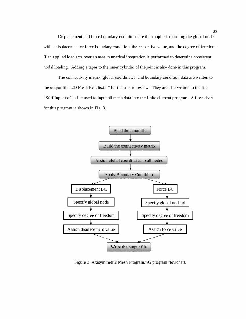
Displacement and force boundary conditions are then applied, returning the global nodes
with a displacement or force boundary condition, the respective value, and the degree of freedom.
If an applied load acts over an area, numerical integration is performed to determine consistent
nodal loading. Adding a taper to the inner cylinder of the joint is also done in this program.
The connectivity matrix, global coordinates, and boundary condition data are written to
the output file “2D Mesh Results.txt” for the user to review. They are also written to the file
“Stiff Input.txt”, a file used to input all mesh data into the finite element program. A flow chart
for this program is shown in Fig. 3.
Figure 3. Axisymmetric Mesh Program.f95 program flowchart.
Read the input file
Displacement BC Force BC
Specify degree of freedom Specify degree of freedom
Specify global node Specify global node id
Assign displacement value Assign force value
Write the output file
Build the connectivity matrix
Assign global coordinates to all nodes
Apply Boundary Conditions
24
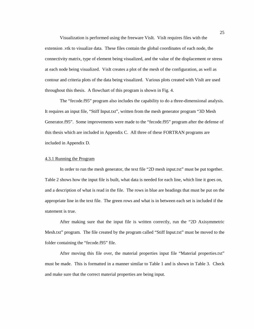
The program “fecode.f95” uses the data from the mesh program to solve for unknown
displacements and perform postprocessing. The file “Stiff Input.txt” from the mesh program is
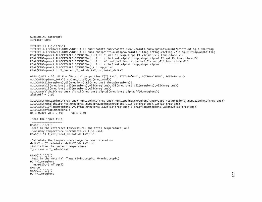
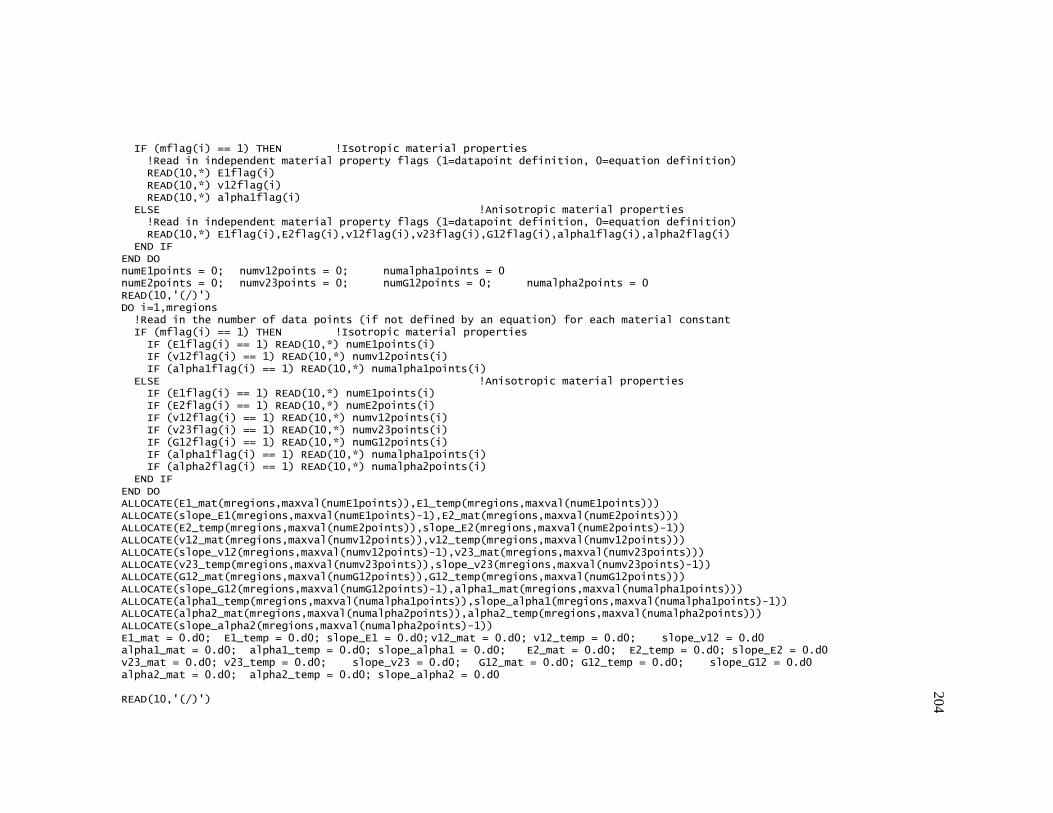
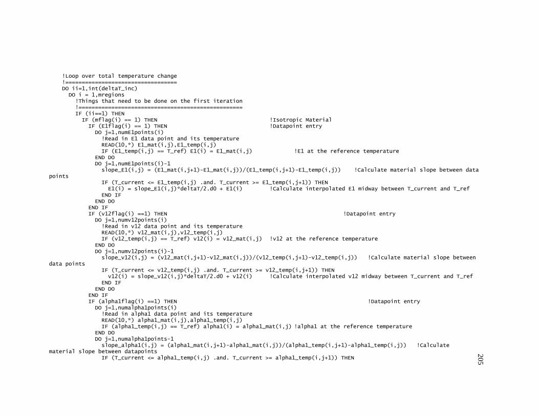
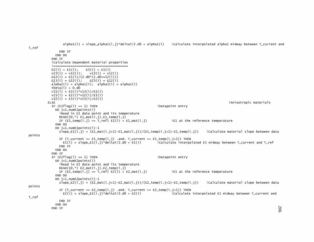
used to read in all mesh data. Material properties are read in from the “Material Properties.txt”
input file. This file contains all independent material property constants for isotropic and
anisotropic materials in the joint. Stiffness and compliance matrices are calculated for each
material, along with off-axis CTEs.
In order to assemble the global stiffness matrix, each element stiffness matrix must be
formed. Shape functions and the determinate of the Jacobian matrix are calculated for each
element and are used in the integration of stiffness values. Stiffness values are integrated using
Gauss quadrature, as discussed in Section 4.2.2. After calculating the stiffness values for each
element, they are added to the global stiffness matrix.
Since the global stiffness matrix is a sparse, banded, symmetric matrix, a more efficient
storage scheme is utilized to store only the upper diagonal of the stiffness matrix. It is stored in a
rectangular matrix with the diagonal stored in the first column. The rectangle has as many rows
as there are total nodal displacements in the model and the width is the half bandwidth of the
square global stiffness matrix. The global force vector is also assembled.
From the input file from the mesh program, the boundary conditions are applied, altering
values in the global force vector and stiffness matrix. Once all the boundary conditions are
applied, the unknown displacements can be solved for. This is done by applying an LU
Decomposition algorithm on the set of equations. The result of this process is a vector containing
the unknown nodal displacements.
Postprocessing is done by calculating stresses and strains at the individual gauss points of
each element, extrapolating them out to the nodes, and averaging nodes within material regions.
Stresses are not averaged across dissimilar material interfaces. Nodal displacements, stresses,
and strains are written to respective output files.
25
Visualization is performed using the freeware VisIt. VisIt requires files with the
extension .vtk to visualize data. These files contain the global coordinates of each node, the
connectivity matrix, type of element being visualized, and the value of the displacement or stress
at each node being visualized. VisIt creates a plot of the mesh of the configuration, as well as
contour and criteria plots of the data being visualized. Various plots created with VisIt are used
throughout this thesis. A flowchart of this program is shown in Fig. 4.
The “fecode.f95” program also includes the capability to do a three-dimensional analysis.
It requires an input file, “Stiff Input.txt”, written from the mesh generator program “3D Mesh
Generator.f95”. Some improvements were made to the “fecode.f95” program after the defense of
this thesis which are included in Appendix C. All three of these FORTRAN programs are
included in Appendix D.
4.3.1 Running the Program
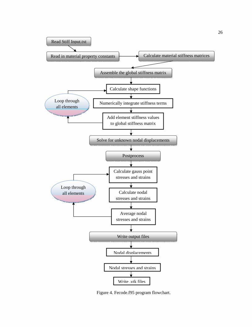
In order to run the mesh generator, the text file “2D mesh input.txt” must be put together.
Table 2 shows how the input file is built, what data is needed for each line, which line it goes on,
and a description of what is read in the file. The rows in blue are headings that must be put on the
appropriate line in the text file. The green rows and what is in between each set is included if the
statement is true.
After making sure that the input file is written correctly, run the “2D Axisymmetric
Mesh.txt” program. The file created by the program called “Stiff Input.txt” must be moved to the
folder containing the “fecode.f95” file.
After moving this file over, the material properties input file “Material properties.txt”
must be made. This is formatted in a manner similar to Table 1 and is shown in Table 3. Check
and make sure that the correct material properties are being input.
26
Figure 4. Fecode.f95 program flowchart.
Read Stiff Input.txt
Read in material property constants Calculate material stiffness matrices
Assemble the global stiffness matrix
Calculate shape functions
Numerically integrate stiffness terms
Add element stiffness values to global stiffness matrix
Solve for unknown nodal displacements
Loop through all elements
Postprocess
Calculate gauss point stresses and strains
Calculate nodal stresses and strains
Average nodal stresses and strains
Loop through all elements
Write output files
Nodal stresses and strains
Nodal displacements
Write .vtk files
27
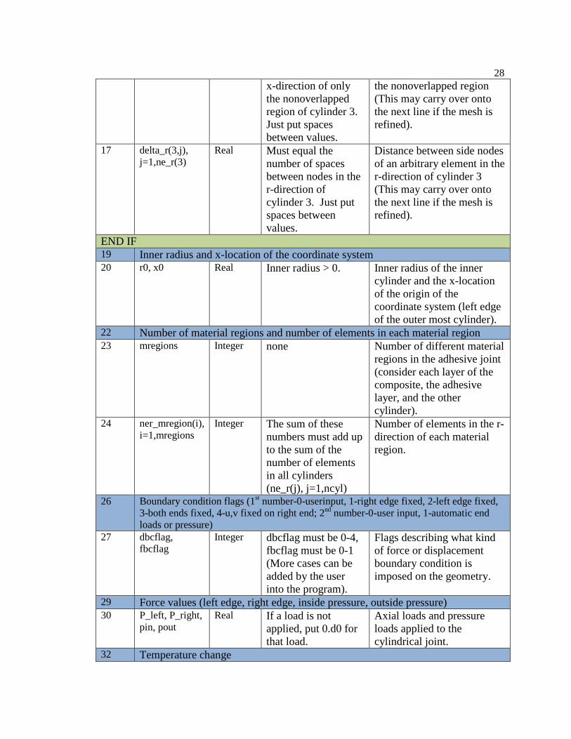
Table 2. Mesh Input File Explanation
Line # Variable Type Limits Description 1 title Character <70 characters Title of program. Enclose in
single brackets. 3 Nodes per element and the total number of cylinders 4 npe Integer 4 or 8 Number of nodes per element. 5 ncyl Integer >1, <3 Number of cylinders. 7 Number of elements in the x- and r-directions of each tube respectively 8 ne_x(1),ne_r(1) Integer none Number of elements in the x-
direction and number of elements in the r-direction
IF ncyl>1 or ncyl>2 THEN 9 ne_x(2),ne_r(2) Integer none Number of elements in the x-
direction and number of elements in the r-direction
10 ne_x(3),ne_r(3) Integer none Number of elements in the x-direction and number of elements in the r-direction
END IF 12 Dimensions of the elements (x and r of cylinder 1, r of cylinder 2, x and r of the
nonoverlapped region of cylinder 3) 13 delta_x(1,j),
j=1,ne_x(1) Real Must equal the
number of spaces between nodes in the x-direction of cylinder 1. Just put spaces between values.
Distance between side nodes of an arbitrary element in the x-direction of cylinder 1 (This may carry over onto the next line if the mesh is refined).
14 delta_r(1,j), j=1,ne_r(1)
Real Must equal the number of spaces between nodes in the r-direction of cylinder 1. Just put spaces between values.
Distance between side nodes of an arbitrary element in the r-direction of cylinder 1 (This may carry over onto the next line if the mesh is refined).
IF ncyl>1 or ncyl>2 THEN 15 delta_r(2,j),
j=1,ne_r(2) Real Must equal the
number of spaces between nodes in the r-direction of cylinder 2. Just put spaces between values.
Distance between side nodes of an arbitrary element in the r-direction of cylinder 2 (This may carry over onto the next line if the mesh is refined).
16 delta_x(3,j), j=1,ne_x(2)
Real Must equal the number of spaces between nodes in the
Distance between side nodes of an arbitrary element in the x-direction of cylinder 3 of
28
x-direction of only the nonoverlapped region of cylinder 3. Just put spaces between values.
the nonoverlapped region (This may carry over onto the next line if the mesh is refined).
17 delta_r(3,j), j=1,ne_r(3)
Real Must equal the number of spaces between nodes in the r-direction of cylinder 3. Just put spaces between values.
Distance between side nodes of an arbitrary element in the r-direction of cylinder 3 (This may carry over onto the next line if the mesh is refined).
END IF 19 Inner radius and x-location of the coordinate system 20 r0, x0 Real Inner radius > 0. Inner radius of the inner
cylinder and the x-location of the origin of the coordinate system (left edge of the outer most cylinder).
22 Number of material regions and number of elements in each material region 23 mregions Integer none Number of different material
regions in the adhesive joint (consider each layer of the composite, the adhesive layer, and the other cylinder).
24 ner_mregion(i), i=1,mregions
Integer The sum of these numbers must add up to the sum of the number of elements in all cylinders (ne_r(j), j=1,ncyl)
Number of elements in the r-direction of each material region.
26 Boundary condition flags (1st number-0-userinput, 1-right edge fixed, 2-left edge fixed, 3-both ends fixed, 4-u,v fixed on right end; 2nd number-0-user input, 1-automatic end loads or pressure)
27 dbcflag, fbcflag
Integer dbcflag must be 0-4, fbcflag must be 0-1 (More cases can be added by the user into the program).
Flags describing what kind of force or displacement boundary condition is imposed on the geometry.
29 Force values (left edge, right edge, inside pressure, outside pressure) 30 P_left, P_right,
pin, pout Real If a load is not
applied, put 0.d0 for that load.
Axial loads and pressure loads applied to the cylindrical joint.
32 Temperature change
29
33 deltat Real If it is a negative temperature change, put a negative sign out front.
Change in temperature from some reference temperature.
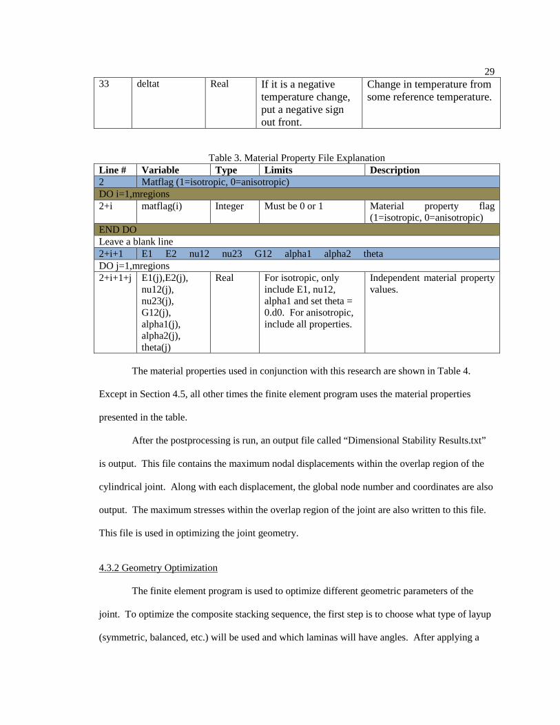
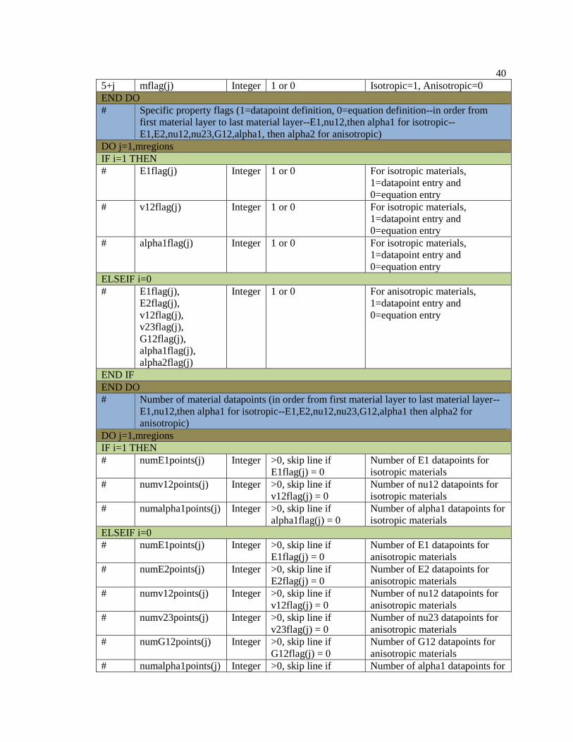
Table 3. Material Property File Explanation Line # Variable Type Limits Description 2 Matflag (1=isotropic, 0=anisotropic) DO i=1,mregions 2+i matflag(i) Integer Must be 0 or 1 Material property flag
(1=isotropic, 0=anisotropic) END DO Leave a blank line 2+i+1 E1 E2 nu12 nu23 G12 alpha1 alpha2 theta DO j=1,mregions 2+i+1+j E1(j),E2(j),
Integer 1 or 0 For anisotropic materials, 1=datapoint entry and 0=equation entry
END IF END DO # Number of material datapoints (in order from first material layer to last material layer--
E1,nu12,then alpha1 for isotropic--E1,E2,nu12,nu23,G12,alpha1 then alpha2 for anisotropic)
DO j=1,mregions IF i=1 THEN # numE1points(j) Integer >0, skip line if
E1flag(j) = 0 Number of E1 datapoints for isotropic materials
# numv12points(j) Integer >0, skip line if v12flag(j) = 0
Number of nu12 datapoints for isotropic materials
# numalpha1points(j) Integer >0, skip line if alpha1flag(j) = 0
Number of alpha1 datapoints for isotropic materials
ELSEIF i=0 # numE1points(j) Integer >0, skip line if
E1flag(j) = 0 Number of E1 datapoints for anisotropic materials
# numE2points(j) Integer >0, skip line if E2flag(j) = 0
Number of E2 datapoints for anisotropic materials
# numv12points(j) Integer >0, skip line if v12flag(j) = 0
Number of nu12 datapoints for anisotropic materials
# numv23points(j) Integer >0, skip line if v23flag(j) = 0
Number of nu23 datapoints for anisotropic materials
# numG12points(j) Integer >0, skip line if G12flag(j) = 0
Number of G12 datapoints for anisotropic materials
# numalpha1points(j) Integer >0, skip line if Number of alpha1 datapoints for
41
alpha1flag(j) = 0 isotropic materials # numalpha2points(j) Integer >0, skip line if
alpha2flag(j) = 0 Number of alpha2 datapoints for isotropic materials
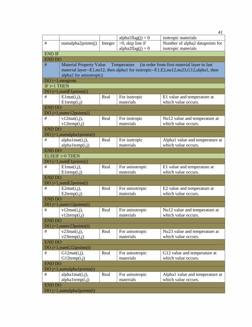
END IF END DO # Material Property Value Temperature (in order from first material layer to last
material layer--E1,nu12, then alpha1 for isotropic--E1,E2,nu12,nu23,G12,alpha1, then alpha2 for anisotropic)
DO i=1,mregions IF i=1 THEN DO j=1,numE1points(i) # E1mat(i,j),
E1temp(i,j) Real For isotropic
materials E1 value and temperature at which value occurs.
END DO DO j=1,numv12points(i) # v12mat(i,j),
v12temp(i,j) Real For isotropic
materials Nu12 value and temperature at which value occurs.
END DO DO j=1,numalpha1points(i) # alpha1mat(i,j),
alpha1temp(i,j) Real For isotropic
materials Alpha1 value and temperature at which value occurs.
END DO ELSEIF i=0 THEN DO j=1,numE1points(i) # E1mat(i,j),
E1temp(i,j) Real For anisotropic
materials E1 value and temperature at which value occurs.
END DO DO j=1,numE2points(i) # E2mat(i,j),
E2temp(i,j) Real For anisotropic
materials E2 value and temperature at which value occurs.
END DO DO j=1,numv12points(i) # v12mat(i,j),
v12temp(i,j) Real For anisotropic
materials Nu12 value and temperature at which value occurs.
END DO DO j=1,numv23points(i) # v23mat(i,j),
v23temp(i,j) Real For anisotropic
materials Nu23 value and temperature at which value occurs.
END DO DO j=1,numG12points(i) # G12mat(i,j),
G12temp(i,j) Real For anisotropic
materials G12 value and temperature at which value occurs.
END DO DO j=1,numalpha1points(i) # alpha1mat(i,j),
alpha1temp(i,j) Real For anisotropic
materials Alpha1 value and temperature at which value occurs.
END DO DO j=1,numalpha2points(i)
42
# alpha2mat(i,j), alpha2temp(i,j)
Real For anisotropic materials
Alpha2 value and temperature at which value occurs.
END DO END IF END DO # Lamina fiber angle—Assumed not to change with temperature (Don’t put anything for
isotropic materials) DO j=1,mregions # theta(j) Real For anisotropic
materials only, put nothing for isotropic.
Fiber angle for composite laminate.
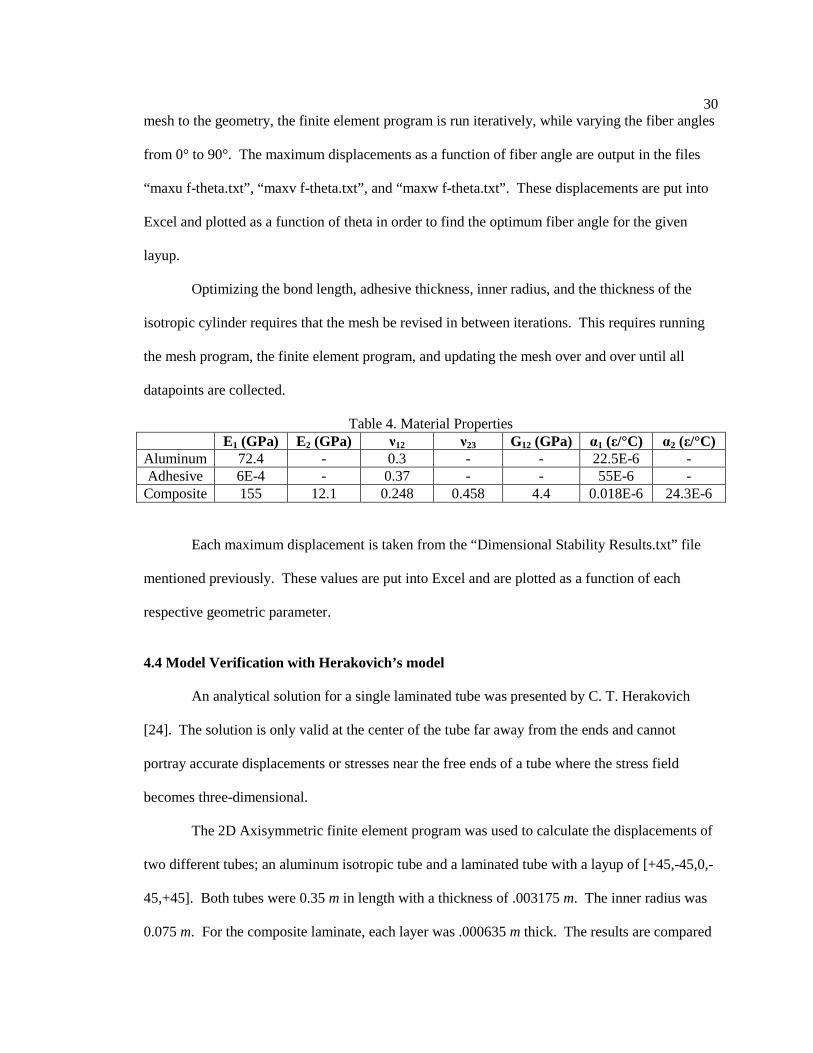
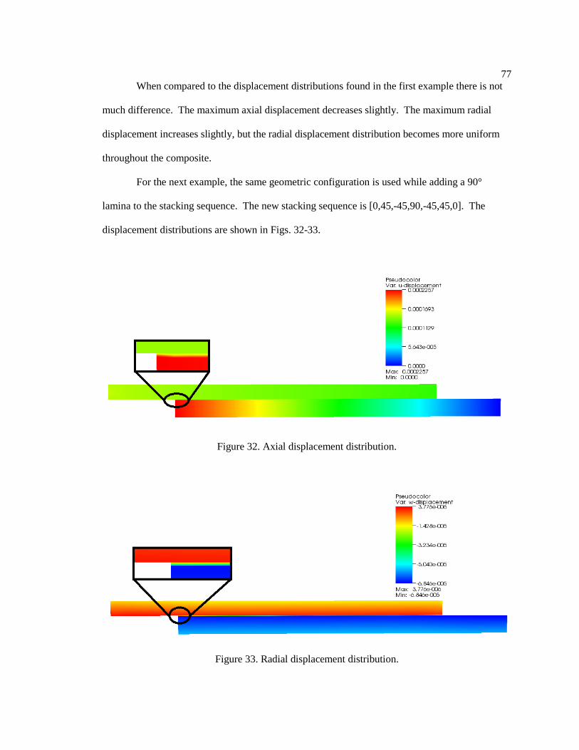
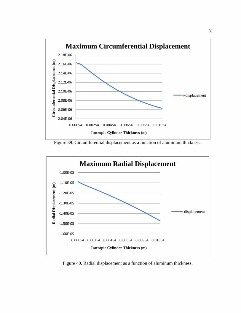
END DO 4.7 Cylindrical Adhesive Joint Design Procedure
When designing cylindrical adhesive joints, the finite element program can be used to
determine the optimum stacking sequence of the composite, the adhesive bond length and
thickness, and the thickness of the isotropic cylinder. This design process can be an iterative
process, depending on the design constraints of the joint. A specific example is shown here of
how to use this joint design procedure; further examples are shown in the appendix.
For this example, the isotropic tube is an aluminum tube of length 0.1 m, inner radius of
0.025 m, and a 0.0054 m wall thickness. The wall thickness will not change for this example.
The applied load is a -100°C temperature change from room temperature. The material properties
used are those given in Section 4.3 and are assumed to remain constant with the changing
temperature.
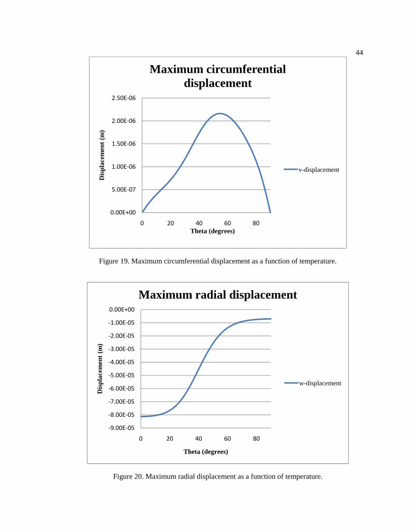
4.7.1 Determine the Optimized Stacking Geometry
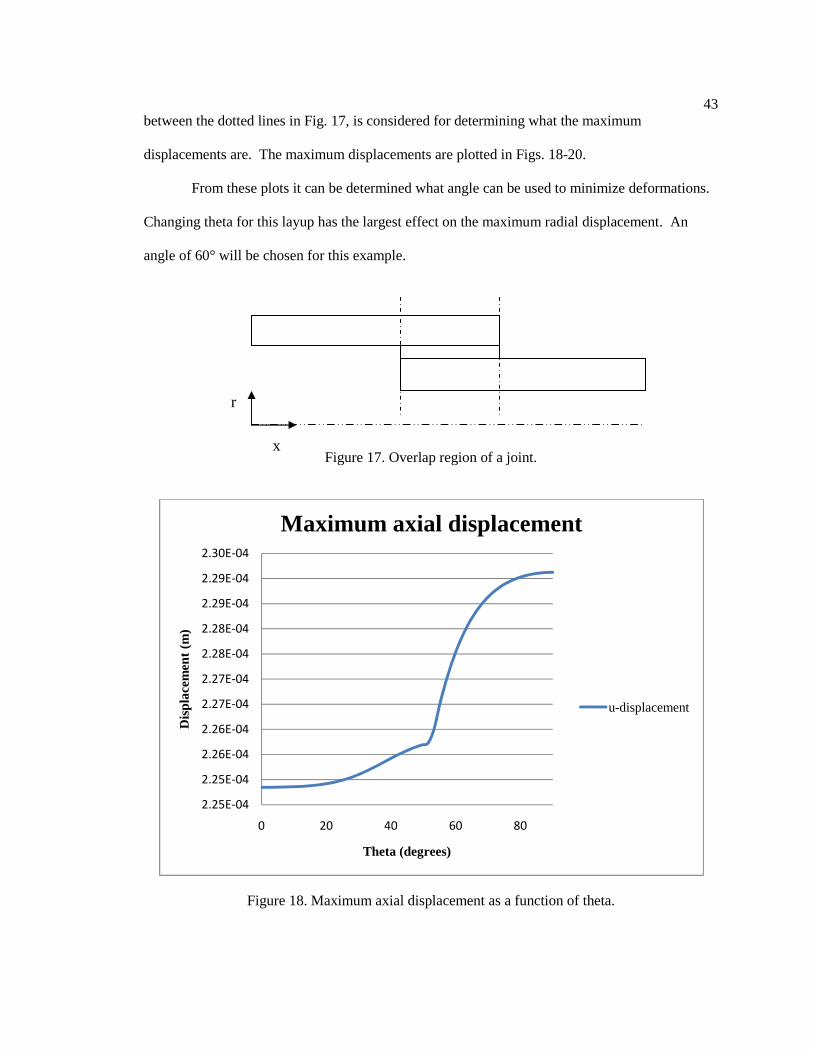
In order to determine the optimal stacking sequence of a [+θ,-θ,0,-θ,+θ] layup for the
composite laminate of a cylindrical adhesive joint, the finite element program is used to
determine the maximum displacements with theta ranging from 0 to 90°. The adhesive thickness
is assumed to be 0.1 mm thick and the bond length is assumed to be 50 mm. Each layer of the
composite is 0.635 mm thick. Only the overlap region of the joint, the portion of the joint
43
x
r
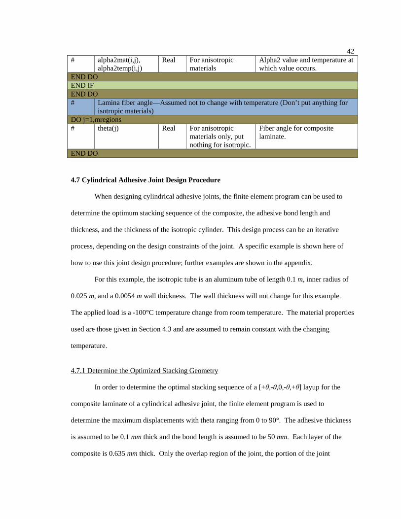
between the dotted lines in Fig. 17, is considered for determining what the maximum
displacements are. The maximum displacements are plotted in Figs. 18-20.
From these plots it can be determined what angle can be used to minimize deformations.
Changing theta for this layup has the largest effect on the maximum radial displacement. An
angle of 60° will be chosen for this example.
Figure 17. Overlap region of a joint.
Figure 18. Maximum axial displacement as a function of theta.
2.25E-04
2.25E-04
2.26E-04
2.26E-04
2.27E-04
2.27E-04
2.28E-04
2.28E-04
2.29E-04
2.29E-04
2.30E-04
0 20 40 60 80
Dis
plac
emen
t (m
)
Theta (degrees)
Maximum axial displacement
u-displacement
44
Figure 19. Maximum circumferential displacement as a function of temperature.
Figure 20. Maximum radial displacement as a function of temperature.
0.00E+00
5.00E-07
1.00E-06
1.50E-06
2.00E-06
2.50E-06
0 20 40 60 80
Dis
plac
emen
t (m
)
Theta (degrees)
Maximum circumferential displacement
v-displacement
-9.00E-05
-8.00E-05
-7.00E-05
-6.00E-05
-5.00E-05
-4.00E-05
-3.00E-05
-2.00E-05
-1.00E-05
0.00E+00
0 20 40 60 80
Dis
plac
emen
t (m
)
Theta (degrees)
Maximum radial displacement
w-displacement
45
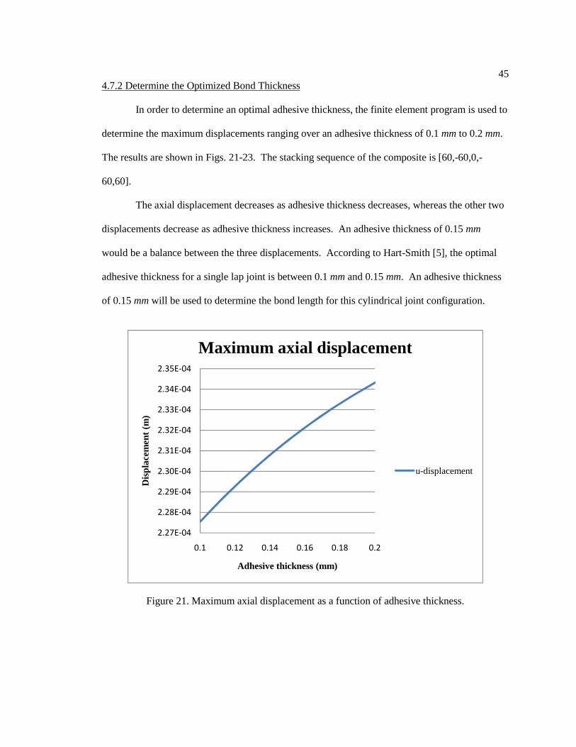
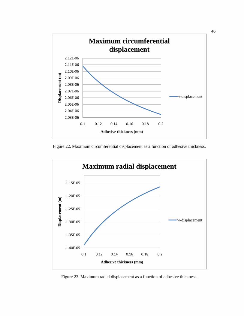
4.7.2 Determine the Optimized Bond Thickness
In order to determine an optimal adhesive thickness, the finite element program is used to
determine the maximum displacements ranging over an adhesive thickness of 0.1 mm to 0.2 mm.
The results are shown in Figs. 21-23. The stacking sequence of the composite is [60,-60,0,-
60,60].
The axial displacement decreases as adhesive thickness decreases, whereas the other two
displacements decrease as adhesive thickness increases. An adhesive thickness of 0.15 mm
would be a balance between the three displacements. According to Hart-Smith [5], the optimal
adhesive thickness for a single lap joint is between 0.1 mm and 0.15 mm. An adhesive thickness
of 0.15 mm will be used to determine the bond length for this cylindrical joint configuration.
Figure 21. Maximum axial displacement as a function of adhesive thickness.
2.27E-04
2.28E-04
2.29E-04
2.30E-04
2.31E-04
2.32E-04
2.33E-04
2.34E-04
2.35E-04
0.1 0.12 0.14 0.16 0.18 0.2
Dis
plac
emen
t (m
)
Adhesive thickness (mm)
Maximum axial displacement
u-displacement
46
Figure 22. Maximum circumferential displacement as a function of adhesive thickness.
Figure 23. Maximum radial displacement as a function of adhesive thickness.
2.03E-06
2.04E-06
2.05E-06
2.06E-06
2.07E-06
2.08E-06
2.09E-06
2.10E-06
2.11E-06
2.12E-06
0.1 0.12 0.14 0.16 0.18 0.2
Dis
plac
emen
t (m
)
Adhesive thickness (mm)
Maximum circumferential displacement
v-displacement
-1.40E-05
-1.35E-05
-1.30E-05
-1.25E-05
-1.20E-05
-1.15E-05
0.1 0.12 0.14 0.16 0.18 0.2
Dis
plac
emen
t (m
)
Adhesive thickness (mm)
Maximum radial displacement
w-displacement
47
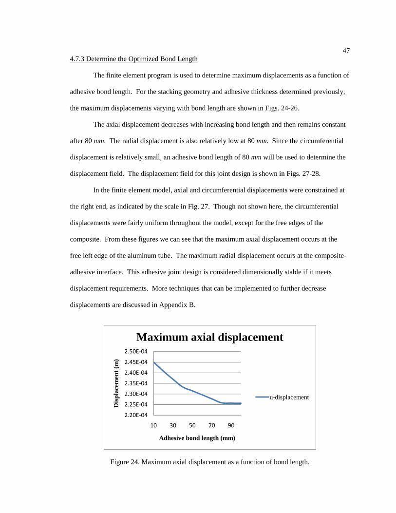
4.7.3 Determine the Optimized Bond Length
The finite element program is used to determine maximum displacements as a function of
adhesive bond length. For the stacking geometry and adhesive thickness determined previously,
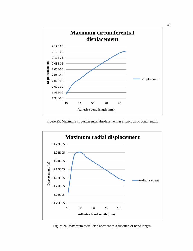
the maximum displacements varying with bond length are shown in Figs. 24-26.
The axial displacement decreases with increasing bond length and then remains constant
after 80 mm. The radial displacement is also relatively low at 80 mm. Since the circumferential
displacement is relatively small, an adhesive bond length of 80 mm will be used to determine the
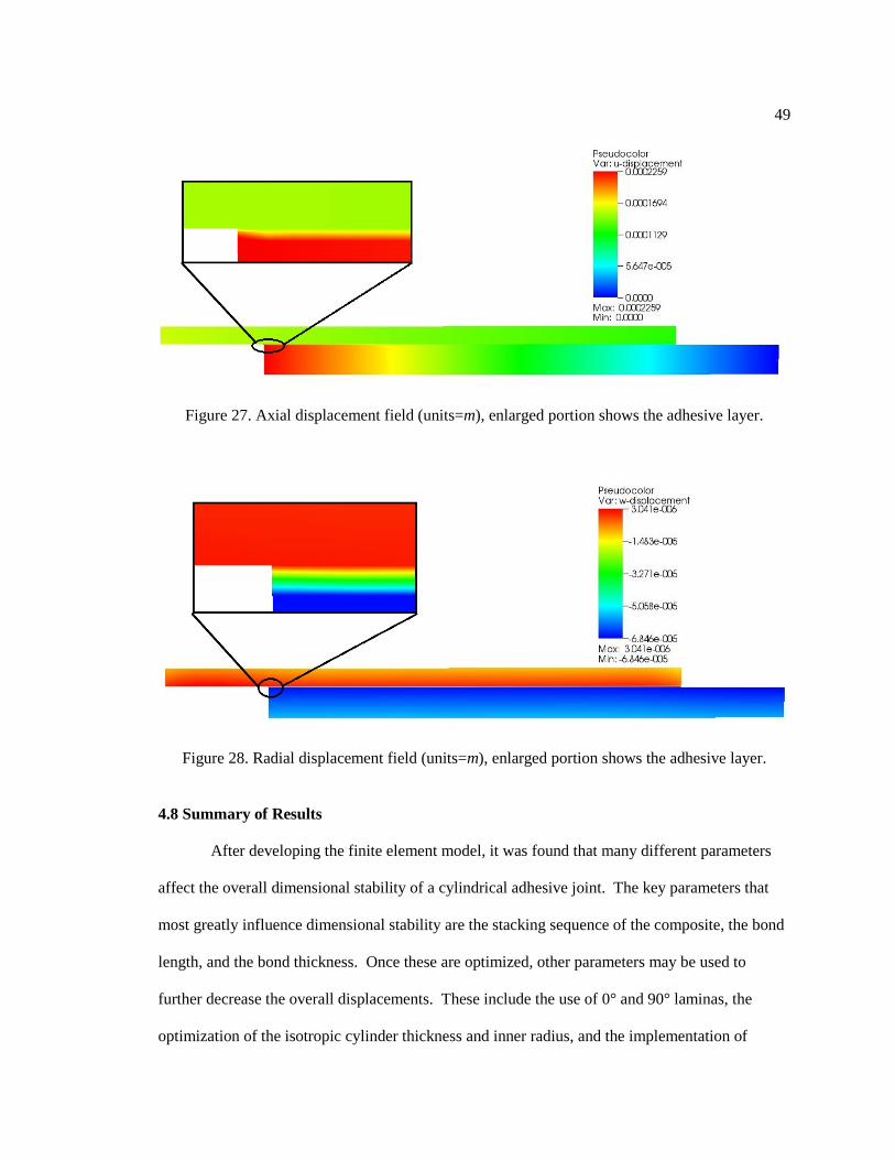
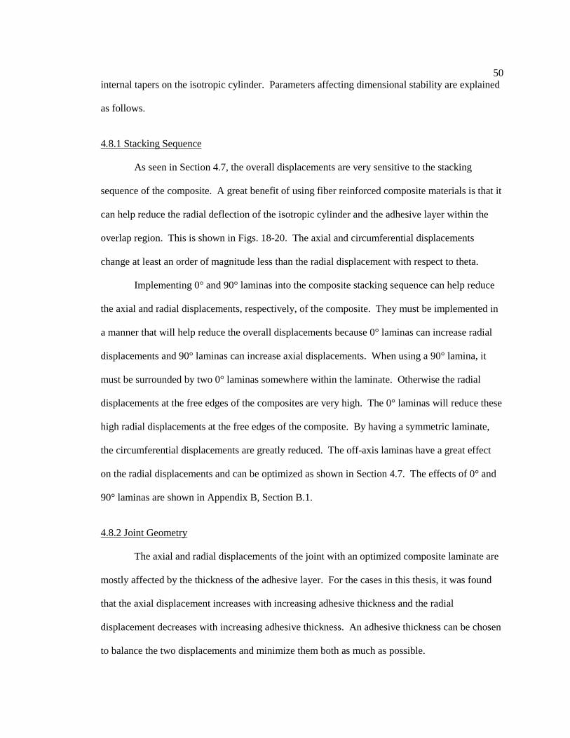
displacement field. The displacement field for this joint design is shown in Figs. 27-28.
In the finite element model, axial and circumferential displacements were constrained at
the right end, as indicated by the scale in Fig. 27. Though not shown here, the circumferential
displacements were fairly uniform throughout the model, except for the free edges of the
composite. From these figures we can see that the maximum axial displacement occurs at the
free left edge of the aluminum tube. The maximum radial displacement occurs at the composite-
adhesive interface. This adhesive joint design is considered dimensionally stable if it meets
displacement requirements. More techniques that can be implemented to further decrease
displacements are discussed in Appendix B.
Figure 24. Maximum axial displacement as a function of bond length.
2.20E-04
2.25E-04
2.30E-04
2.35E-04
2.40E-04
2.45E-04
2.50E-04
10 30 50 70 90
Dis
plac
emen
t (m
)
Adhesive bond length (mm)
Maximum axial displacement
u-displacement
48
Figure 25. Maximum circumferential displacement as a function of bond length.
Figure 26. Maximum radial displacement as a function of bond length.
1.96E-06
1.98E-06
2.00E-06
2.02E-06
2.04E-06
2.06E-06
2.08E-06
2.10E-06
2.12E-06
2.14E-06
10 30 50 70 90
Dis
plac
emen
t (m
)
Adhesive bond length (mm)
Maximum circumferential displacement
v-displacement
-1.29E-05
-1.28E-05
-1.27E-05
-1.26E-05
-1.25E-05
-1.24E-05
-1.23E-05
-1.22E-05
10 30 50 70 90
Dis
plac
emen
t (m
)
Adhesive bond length (mm)
Maximum radial displacement
w-displacement
49
Figure 27. Axial displacement field (units=m), enlarged portion shows the adhesive layer.
Figure 28. Radial displacement field (units=m), enlarged portion shows the adhesive layer.
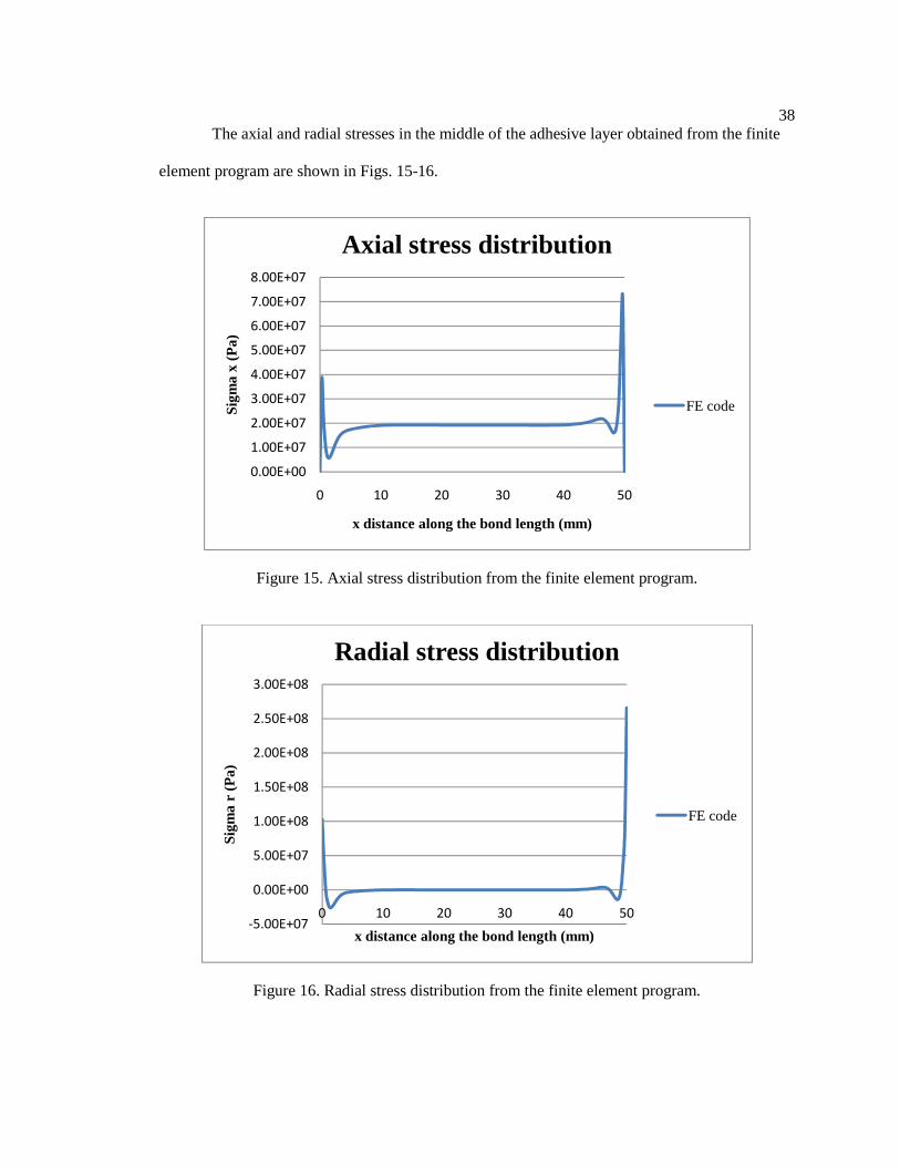
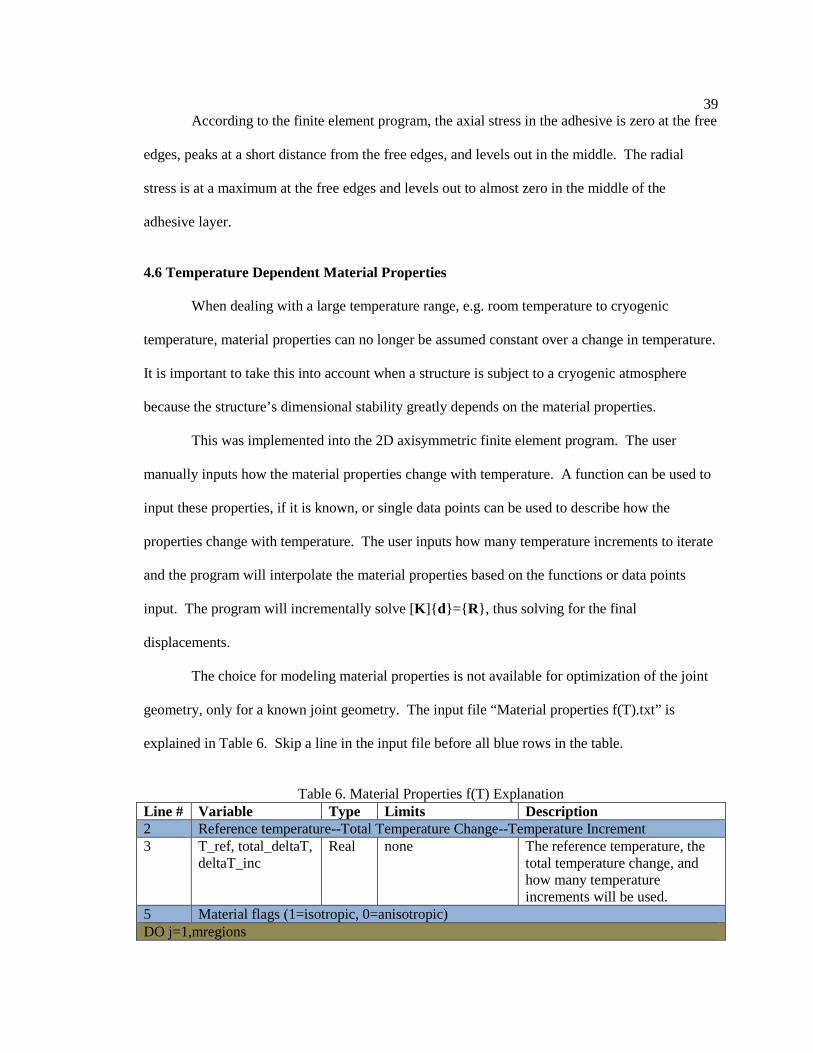
4.8 Summary of Results
After developing the finite element model, it was found that many different parameters
affect the overall dimensional stability of a cylindrical adhesive joint. The key parameters that
most greatly influence dimensional stability are the stacking sequence of the composite, the bond
length, and the bond thickness. Once these are optimized, other parameters may be used to
further decrease the overall displacements. These include the use of 0° and 90° laminas, the
optimization of the isotropic cylinder thickness and inner radius, and the implementation of
50
internal tapers on the isotropic cylinder. Parameters affecting dimensional stability are explained
as follows.
4.8.1 Stacking Sequence
As seen in Section 4.7, the overall displacements are very sensitive to the stacking
sequence of the composite. A great benefit of using fiber reinforced composite materials is that it
can help reduce the radial deflection of the isotropic cylinder and the adhesive layer within the
overlap region. This is shown in Figs. 18-20. The axial and circumferential displacements
change at least an order of magnitude less than the radial displacement with respect to theta.
Implementing 0° and 90° laminas into the composite stacking sequence can help reduce
the axial and radial displacements, respectively, of the composite. They must be implemented in
a manner that will help reduce the overall displacements because 0° laminas can increase radial
displacements and 90° laminas can increase axial displacements. When using a 90° lamina, it
must be surrounded by two 0° laminas somewhere within the laminate. Otherwise the radial
displacements at the free edges of the composites are very high. The 0° laminas will reduce these
high radial displacements at the free edges of the composite. By having a symmetric laminate,
the circumferential displacements are greatly reduced. The off-axis laminas have a great effect
on the radial displacements and can be optimized as shown in Section 4.7. The effects of 0° and
90° laminas are shown in Appendix B, Section B.1.
4.8.2 Joint Geometry
The axial and radial displacements of the joint with an optimized composite laminate are
mostly affected by the thickness of the adhesive layer. For the cases in this thesis, it was found
that the axial displacement increases with increasing adhesive thickness and the radial
displacement decreases with increasing adhesive thickness. An adhesive thickness can be chosen
to balance the two displacements and minimize them both as much as possible.
51
For an optimized composite laminate, all displacements are affected by the bond length
of the joint. The axial and radial displacements can be minimized with longer bond lengths
whereas the circumferential displacement is minimal for shorter bond lengths. A balance can be
found to relatively minimize all displacements. The circumferential displacement is small
compared to the other two, so another option would be to choose a bond length to reduce the axial
and radial deformation.
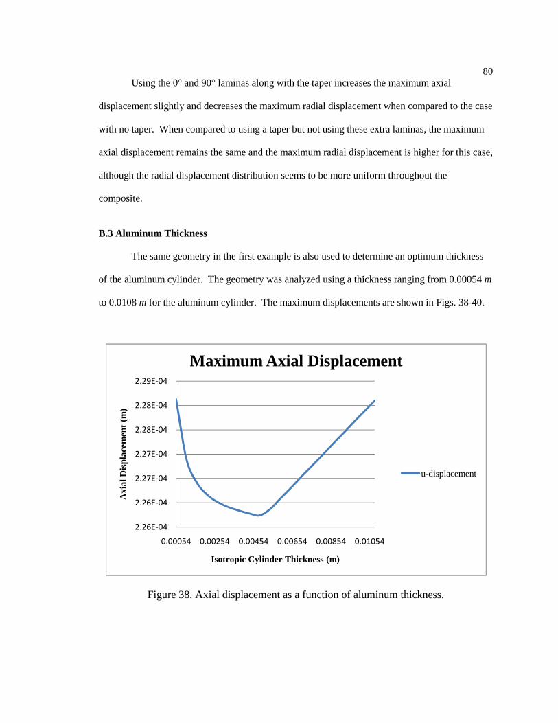
The thickness of the isotropic tube also has an effect on the dimensional stability of
cylindrical adhesive joints. It is shown in Appendix B, Section B.3 that the axial deformation of a
thin-walled cylinder decreases as the thickness increases. As the cylinder becomes a thick-walled
cylinder, the axial displacement increases as the tube thickness increases.
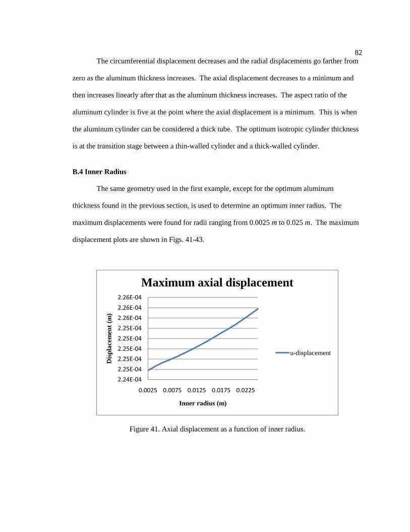
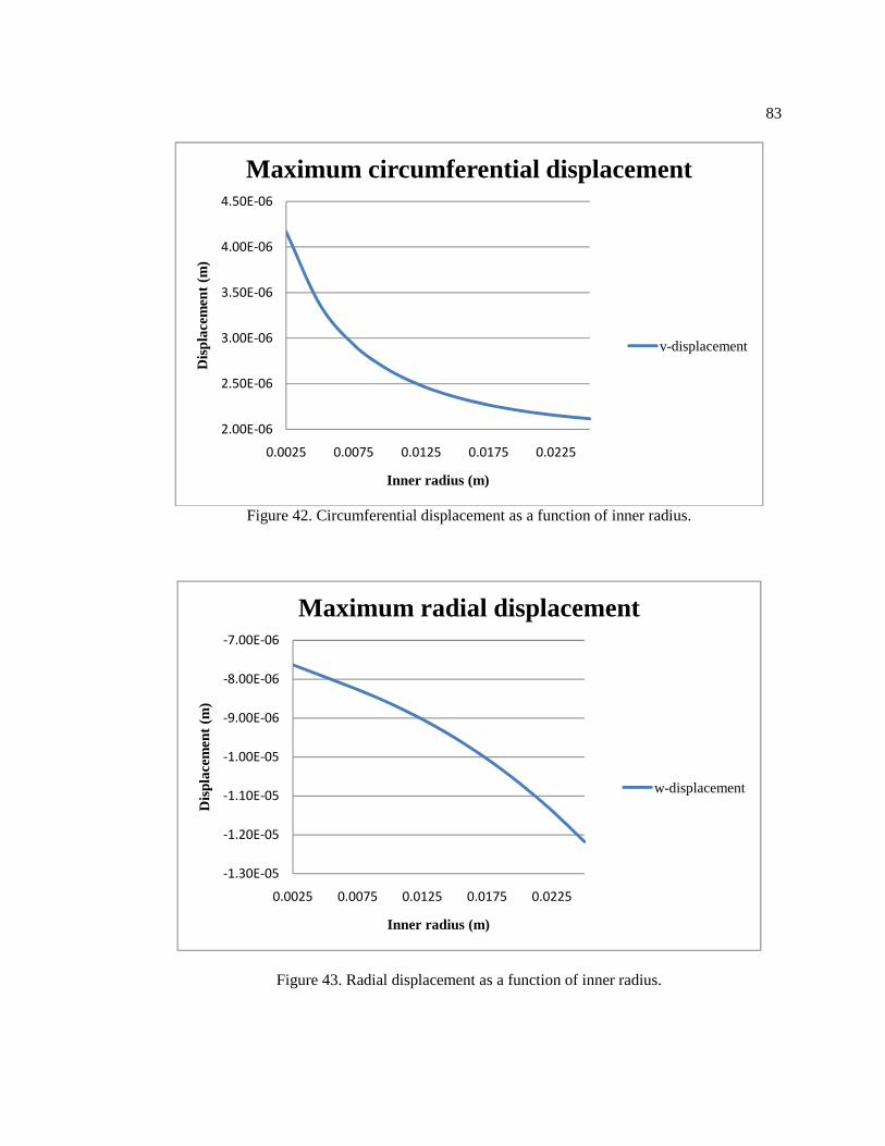
The inner radius of the joint also has an effect on the overall dimensional stability. The
results of how the displacements change as a function of inner radius are shown in Section B.4 of
Appendix B. The inner radius of the joint must be balanced with the thickness of the isotropic
cylinder. As long as the aspect ratio is such that the cylinder is somewhat balanced between a
thick-walled and a thin-walled cylinder, the displacements will be reduced.
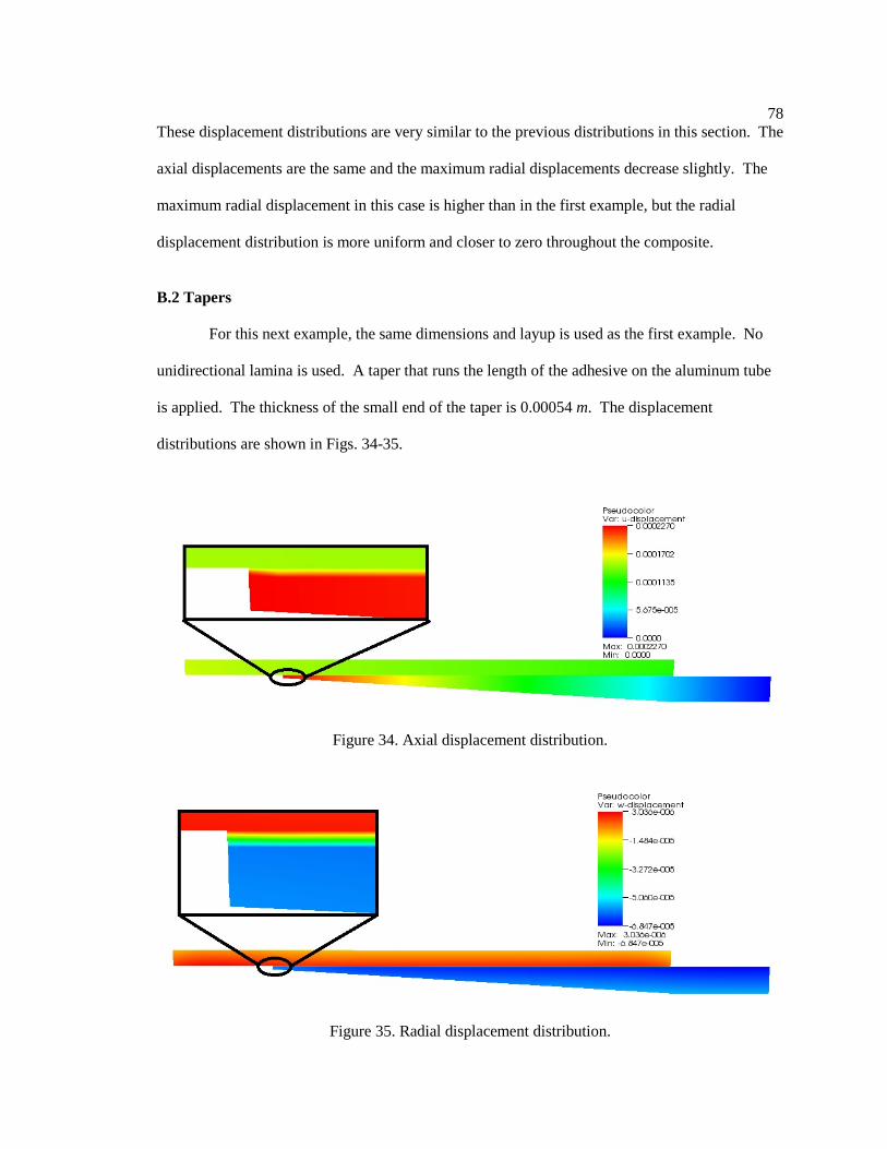
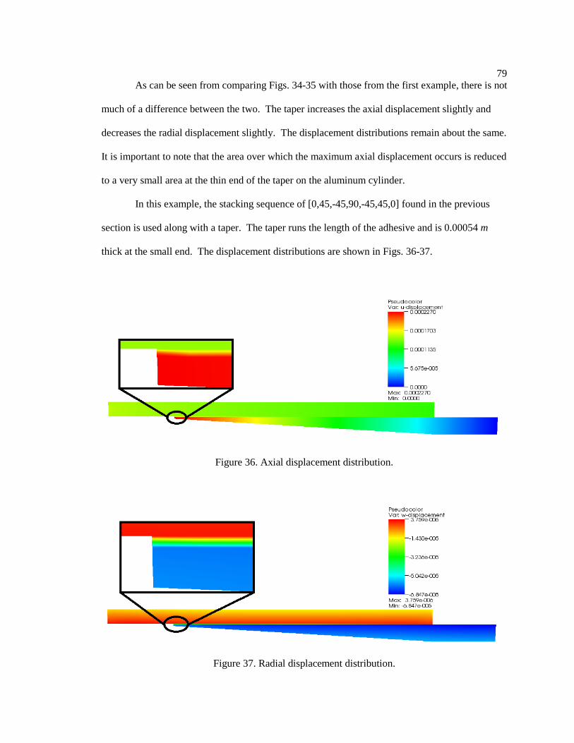
4.8.3 Internal Tapers
Implementing a taper on the inside edge of an isotropic cylinder has various effects on
the displacements of an adhesive joint. For the cases in Appendix B, Section B.2, the maximum
axial displacement increases slightly and the maximum radial displacement decreases slightly.
The total area that the maximum displacement acts over is reduced considerably because it is
located on the thinnest part of the taper.
4.9 Recommendations for Future Work
The finite element model can serve as a foundation for cylindrical adhesive joint design
based on dimensional stability. The next step that can be taken with this research is testing to
52
verify the accuracy of the model. Due to the inability to characterize the material properties of
the carbon fiber prepreg or the adhesives contained in the materials lab at USU, no type of testing
was performed in conjunction with this research to verify the model. Once materials are procured
and correct material properties are characterized, various types of testing can be performed in
order to verify actual displacement and stress values or to verify displacement and stress trends
predicted by the model.
Several improvements can be made to the model. Using the rectangular storage scheme
for the global stiffness matrix improves computer runtime, but runtime can be improved even
further by implementing a Skyline storage scheme. Also, in order to refine a mesh in the current
model, a completely new mesh must be built by the user. An automatic mesh refinement option
can avoid the need to tediously build a new refined mesh with the same dimensions as the course
mesh. A Graphical User Interface (GUI) can also be implemented to aid the user in building the
model instead of using text files.
Further funding has been provided by SDL that will be used to accomplish testing and
make the suggested improvements to the finite element model. A finite element model will be
developed for a thermal conductivity analysis, and another finite element model will be
developed for square tubular joints. Various adhesive joint configurations (other than cylindrical)
will also be designed.
In conclusion, it is hoped that the research contained in this thesis will benefit the future
research and work of students, faculty, and engineers in the design and development of adhesive
joints based on dimensional stability.
53
REFERENCES [1] Volkersen, O., 1938, “Rivet Strength Distribution in Tensile Stressed Rivet Joints with
Constant Cross Section,” Luftfehrforschung, 15, pp. 41-47. [2] Goland, M., and Reissner, E., 1944, “The Stresses in Cemented Joints,” J. Appl. Mechanics
Trans. ASME, 66, pp. A17-A27. [3] Hart-Smith, L.J., 1973, “Adhesive Bonded Single Lap Joints,” NASA Report Number: NAS1-
CR-112236, NASA Technical Reports Server. [4] Hart-Smith, L.J., 1974, “Analysis and Design of Advanced Composite Bonded Joints,” NASA
Report Number: NASA-CR-2218, NASA Technical Reports Server. [5] Hart-Smith, L.J., 1973, “Adhesive Bonded Double Lap Joints,” NASA Contract Number:
NAS1-11234, NASA Technical Reports Server. [6] Hart-Smith, L.J., 1973, “Non-Classical Adhesive-Bonded Joints in Practical Aerospace
Construction,” NASA Report No. CR-112238, NASA Technical Reports Server. [7] Crocombe, A.D., and Bigwood, D.A., 1989, “Elastic Analysis and Engineering Design
Formulae for Bonded Joints,” Int. J. Adhesion and Adhesives, 9, pp. 229-242. [8] Renton, J.W., and Vinson, J.R, 1975, “The Efficient Design of Adhesive Bonded Joints,” J.
Adhesion, 7, pp. 175-193. [9] Renton, J. W., 1974, “The Analysis and Design of Composite Material Bonded Joints under
Static and Fatigue Loadings,” Ph.D. dissertation, University of Delaware, Newark, DE. [10] Nemes, O., Lachuad, F., and Mojtabi, A., 2007, “Contribution to the Study of Cylindrical
Adhesive Joining,” Int. J. Adhesion and Adhesives, 26, pp. 474-480. [11] Shi, Y.P., and Cheng, S., 1993, “Analysis of Adhesive-Bonded Cylindrical Lap Joints
Subjected to Axial Load,” J. Engineering Mechanics, 119, pp. 584-602. [12] Bartoszyk, A., Johnston, J., Kaprielian, C., Kuhn, J., Kunt, C., Rodini, B., and Young, D.,
1990, “Design/Analysis of the JWST ISIM Bonded Joints for Survivability at Cryogenic Temperatures,” NASA Document ID 20050214411, NASA Technical Reports Server.
[13] Cifie, E., Matzinger, L., Kuhn, J., Fan, T., 2004, “JWST ISIM Distortion Analysis
Challenge,” NASA Document ID 20040082141, NASA Technical Reports Server.
54
[14] Hylands, R. W., 1982, “Strength Characteristics of Mono and Multiple-Wire Steel to Steel Joints Bonded with an Epoxy Adhesive,” Adhesive Joints: Formation, Characteristics, and Testing, Plenum Press, New York, pp. 165-194.
[15] Anderson, G. P., DeVries, K. L., and Sharon, G., 1982, “Evaluation of Adhesive Test
Methods,” Adhesive Joints: Formation, Characteristics, and Testing, Plenum Press, New York, pp. 269-288.
[16] Shimoda, T., He, J., and Aso, S., 2006, “Study of Cryogenic Mechanical Strength and
Fracture Behavior of Adhesives for CFRP Tanks of Reusable Launch Vehicles,” 1, Memoirs of the Faculty of Engineering, Kyushu University, 66, pp. 55-70.
[17] Baldan, A., 2004, “Adhesively-Bonded Joint in Metallic Alloys, Polymers and Composite
Materials: Mechanical and Environmental Durability Performance,” J. Materials Science, 39, pp. 4729-4797.
[18] Renton, J.W., and Vinson, J.R., 1975, “On the Behavior of Bonded Joints in Composite
Material Structures,” Engineering Fracture Mechanics, 7, pp. 41-60. [19] Kim, T., Kweon, J., and Choi, J., 2008, “An Experimental Study on the Effect of Overlap
Length on the Failure of Composite to Aluminum Single Lap Bonded Joints,” J. Reinforced Plastics and Composites, 27, pp. 1071-1082.
“Understanding and Control af Adhesive Crack Propagation in Bonded Joints Between Carbon Fibre Composite Adherends – I. Experimental,” Int. J. Adhesion and Adhesives, 21, pp. 435-443.
[21] Graf, N.A., Schieleit, G. F., and Biggs, R., “Adhesive Bonding Characterization of
Composite Joints for Cryogenic Use,” NASA Report Number NCC8-116, NASA Technical Reports Server.
[22] Cook, R., Malkus, D., Plesha, M., and Witt, R., 2002, Concepts and Applications of Finite
Element Analysis, John Wiley & Sons Inc., Hoboken, NJ, pp. 206, 214, Chap. 6. [23] Cook, R., Malkus, D., Plesha, M., and Witt, R., 2002, Concepts and Applications of Finite
Element Analysis, John Wiley & Sons Inc., Hoboken, NJ, pp. 209, Chap. 6. [24] Herakovich, C. T., 1997, Mechanics of Fibrous Composites, John Wiley & Sons Inc.,
Hoboken, NJ, pp. 362-378, Chap. 10. [25] Boresi, A.P., and Schmidt, R.J., 2003, Advanced Mechanics of Materials, John Wiley &
Sons Inc., Hoboken, NJ, pp. 1, Chap. 1.
55
[26] Seong, M., Kim, T., Nguyen, K.,Kweon, J., and Choi, J., 2008 “A Parametric Study on the
Failure of Bonded Single-Lap Joints of Carbon Composite and Aluminum,” Composite Structures, 86, pp. 135–145.
[27] Melcher, R.J., and Johnson, W.S., 2007, “Mode I Fracture Toughness of an Adhesively
Bonded Composite–Composite Joint in a Cryogenic Environment,” Composites Science & Technology, 67, pp. 501-506.
[28] Sang-Guk Kang, Myung-Gon Kim, and Chun-Gon Kim, 2007, “Evaluation of Cryogenic
Performance of Adhesives Using Composite-Aluminum Double-Lap Joints,” J. Composite Structures, 78, pp. 440-446.
[29] Gilibert, Y., and Verchery, G., 1982, “Influence of surface Roughness on Mechanical
Properties,” Adhesive Joints: Formation, Characteristics, and Testing, Plenum Press, New York, pp. 69-84.
[30] Venables, J. D., 1982, “Adhesion and Durability of Metal/Polymer Bonds,” Adhesive Joints:
Formation, Characteristics, and Testing, Plenum Press, New York, pp. 453-468. [31] Lawcock, G., Ye, L., Mai, Y., and Sun, C., 1997, “The Effect of Adhesive Bonding Between
Aluminum and Composite Prepeg on the Mechanical Properties of Carbon Fiber Reinforced Metal Laminates,” Composites Science and Technology, 57, pp. 35-35.
[32] Minford, J. D., 1982, “Comparative Study of Aluminum Joint Strength and Durability with
Varying Thickness, Boehmite-Type Oxide Surfaces,” Adhesive Joints: Formation, Characteristics, and Testing, Plenum Press, New York, pp. 503-522.
[33] Clark, E. A., 2009, “The Cryogenic Bonding Evaluation at the Metallic-Composite Interface
of a Composite Overwrapped Pressure Vessel with Additional Impact Investigation,” Master’s thesis, Utah State University, Logan, UT.
[34] Halliday, S. T., Banks, W. M., and Pethrick, R. A., 1999, “Influence of Humidity on the
Durability of Adhesively Bonded Aluminium Composite Structures,” Institution of Mechanical Engineers—Part L, 213, pp. 27-35.
[35] Silva, L., and Adams, R.D., 2007, “Techniques to Reduce the Peel Stresses in Adhesive
Joints with Composites,” Int. J. Adhesion and Adhesives, 27, pp. 227-235. [36] Salimi, A., Omidian, H., and Zohuriaan-Mehr, M.J., 2003, “Mechanical and Thermal
Behavior of Modified Epoxy-Novolak Film Adhesives,” J. Adhesion Science & Technology, 17 (13), pp. 107-123.
56
[37] Timmerman J. F., Hayes, B. S., and Seferis, J.C., 2002, “NanoclayReinforcements Effects on the Cryogenic Microcracking of Carbon Fiber/Epoxy Composites,” Composites Science and Technology, 62, pp. 1249-1258.
[38] Kim, B. C., Park, W., and Lee, D. G., 2008, “Fracture Toughness of Nano-Particle
Reinforced Epoxy Composite,” J. Composite Structures, 86, pp. 69-77. [39] Park, S. W., and Lee, D.G., 2009, “Strength of Double Lab Joints Bonded with Carbon
Black Reinforced Adhesive Under Cryogenic Environment,” J. Adhesion Science and Technology, 23, pp. 619-638.
[40] Hu, X., and Huang, P., 2004, “Study on the Phase Behavior of a Toughened Epoxy
Adhesiveand its Bond-Strength Properties at Liquid Nitrogen Temperature,” J. Adhesion Science & Technology, 18, pp. 807-815.
[41] Hu, X., and Huang, P., 2005, “Influence of Polyether Chain and Synergetic Effect of Mixed
Resins with Different Functionality on Adhesion Properties Of Epoxy Adhesives,” Int. J. Adhesion and Adhesives, 25, pp. 296-300.
[42] Lee, K.H., and Lee, D. G., 2008, “Smart Cure Cycles for the Adhesive Joint of Composite
Structures at Cryogenic Temperatures,” Composite Structures, 86, pp. 37-44. [43] Silva, L., and Adams, R.D., 2007, “Adhesive Joints at High and Low Temperatures Using
Similar and Dissimilar Adherends and Dual Adhesives,” Int. J. Adhesion and Adhesives, 27, pp. 216-226.
[44] Silva, L., Neves, P.J.C. , Adams, R.D., and Spelt, J.K., 2009, “Analytical Models of
Adhesively Bonded Joints – Part I: Literature Survey,” Int. J. Adhesion and Adhesives, 29, pp. 319-330.
[45] Silva, L.,Neves, P. J.C., Adams, R.D., Wang, A., and Spelt, J.K., 2009, “Analytical Models
of Adhesively Bonded Joints – Part II: Comparative Study,” Int. J. Adhesion and Adhesives, 29, pp. 331-341.
[46] Tsai, M.Y., Oplinger, D.W., and Morton, J., 1998, “Improved Theoretical Solutions for
Adhesive Lap Joints,” Int. J. Solids Structures, 35, pp. 1163-1185. [47] Allman, D.J., 1977, “A Theory for Elastic Stresses in Adhesive Bonded Lap Joints,”
Quarterly J. Mechanics and Applied Mathematics, 30, pp. 415-436. [48] Adams, R.D., and Mallick, V., 1992, “A Method for Stress Analysis of Lap Joints,” J.
Adhesion, 38, pp. 199-217.
57
[49] Crocombe, A.D., and Bigwood, D.A., 1990, “Non-Linear Adhesive Bonded Joint Design Analyses,” Int. J. Adhesion and Adhesives, 10, pp. 31-41.
[50] Teodosiadis, R., 1969, “Plastic Analysis of Bonded Composite Lap Joints,” Douglas Aircraft
Company Report Number DAC-67836, Douglas Aircraft Company. [51] Amijima, S., and Fuji, T., 1989, “Extension of One-Dimensional Finite Element Model
Program for Analyzing Elastic-Plastic Stresses and Progressive Failure of Adhesive Bonded Joints,” Int. J. Adhesion and Adhesives, 9, pp. 243-250.
[52] Whitley, K.S., and Gates, T.S., 2004, “Tensile Properties of Polymeric Matrix Composites,”
NASA Document ID 20040086005, NASA Technical Reports Server. [53] Mohling, R.A., Marquardt, E.D., Fusilier, F.C., and Fesmire, J.E., 2003, “Cryogenic
Information Center,” NASA Report No. ICR-0633, NASA Technical Reports Server. [54] Cryogenic Technologies Group website. National Institute of Standards and Technology.
Website found in July 2009. URL http://www.cryogenics.nist.gov/ [55] Marquardt, E. D., Le, J. P., and Radebaugh, R., 2000, “Cryogenic Material Properties
Database,” 11th International Cryocooler Conference, Keystone, pp. 1-7. [56] Silva, L.F.M., and Adams, R.D., 2005, “Measurement of the Mechanical Properties of
Structural Adhesives in Tension and Shear over a Wide Range of Temperatures,” J. Adhesion Science and Technology, 19, pp. 109-141.
[57] Boyd, S. W., Dulieu-Barton, J. M., and Rumsey L., 2006, “Stress Analysis of Finger Joints
in PultrudedGRP Materials,” Int. J. Adhesion & Adhesives, 26, pp. 498–510. [58] Derujinsky, G, 1990, “Integral Seamless Composite Bicycle Frame,” U.S. Patent No.
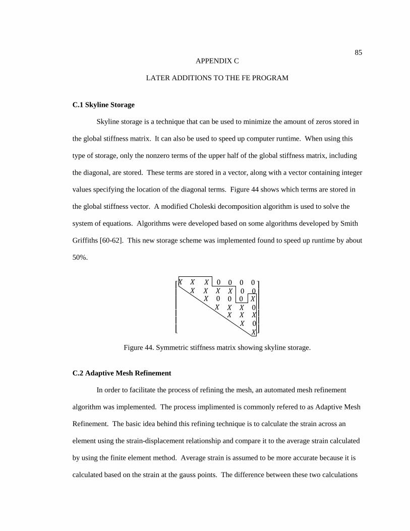
In order to facilitate the process of refining the mesh, an automated mesh refinement
algorithm was implemented. The process implimented is commonly refered to as Adaptive Mesh
Refinement. The basic idea behind this refining technique is to calculate the strain across an
element using the strain-displacement relationship and compare it to the average strain calculated
by using the finite element method. Average strain is assumed to be more accurate because it is
calculated based on the strain at the gauss points. The difference between these two calculations
86
serves as the basis for mesh refinement. As the mesh is refined, the difference between the two
strain values will become smaller and smaller.
Two energy norms are calculated, one being the global strain energy norm and is defined
as follows.
iji% ? 5klmSn`obklmS8;pSP$ (65)
The other energy norm, known as the global energy error norm, serves as the difference between
the smoothed strain field and the strain field calculated from the strain-displacement relationship.
It is defined as follows.
iRi% ? 51klqmS klmS2n`ob1klqmS klmS28;pSP$ (66)
where klqmS is the smoothed strain field for the ith element and klmS is the strain field calculated
from the strain displacement relationship for the ith element, and [E] is the material stiffness
matrix. The relative error η is defined as follows.
[ r iRi%iji% iRi%s$/% (67)
This relative error corresponds to the klmS strain field and can give an idea of which elements
need to be refined. The acceptable error is usually taken to be less than 5%.
Adaptive mesh refinement is helpful in that it automatically finds where the mesh needs
to be refined, converging on the high stress-concentrated areas, since more elements are needed
where the stresses peak. In order to implement this mesh refinement technique, an allowable
global energy error norm, defined as the following.
87
iRiuvv [uvv riji% iRi%0 s$/% (68)
where the allowable relative error is usally taken to be 5%. The total number of elements is
defined as m. The ratio of the actual global energy error norm, Eq. (66), to the allowable energy
norm, Eq. (68) is defined as follows.
ZS iRiSiRiuvv (69)
If ZS is less than unity, the element is larger than it needs to be, but in the finite element program,
nothing was done to change the size of the element. If ZS is greater than unity, it means that more
elements are needed in this region. In the finite element program, an algorithm was developed to
split up elements where ZS is greater than unity. The benefit of this kind of mesh refinement is
that the engineer can analyze a geometry without having to know exactly where the high stress
concentrations are located.
88
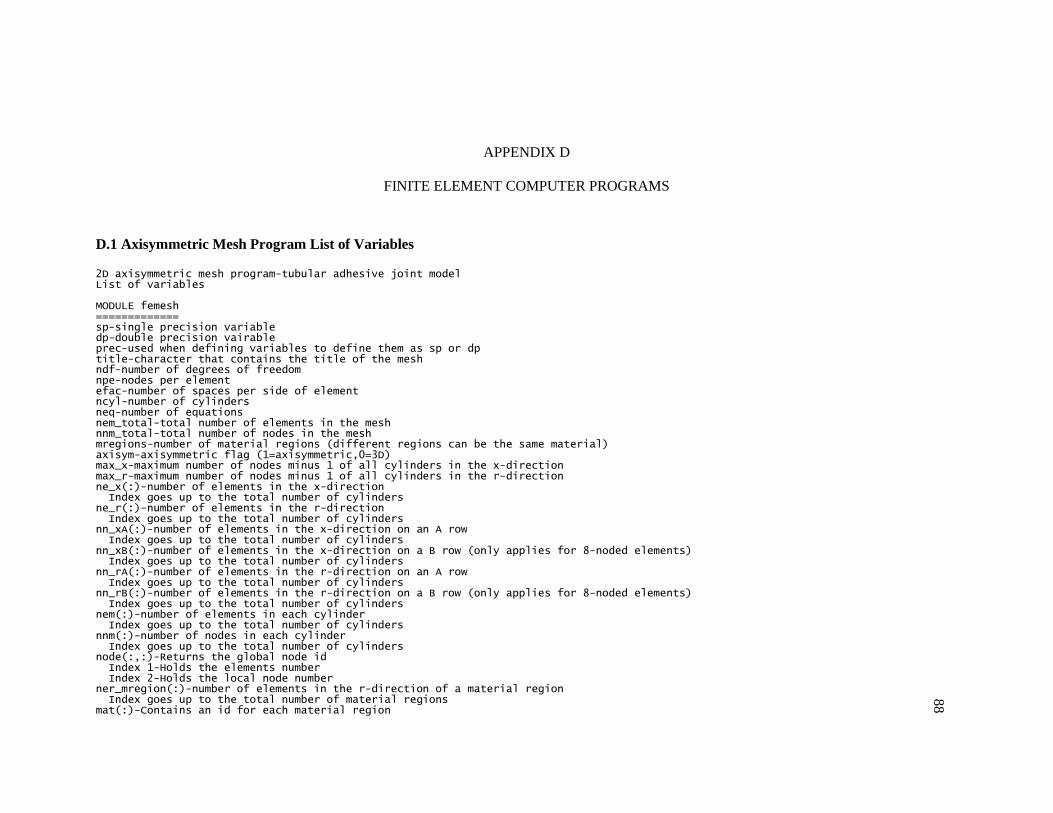
APPENDIX D
FINITE ELEMENT COMPUTER PROGRAMS D.1 Axisymmetric Mesh Program List of Variables
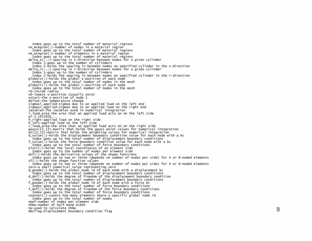
2D axisymmetric mesh program-tubular adhesive joint model List of variables MODULE femesh ============= sp-single precision variable dp-double precision vairable prec-used when defining variables to define them as sp or dp title-character that contains the title of the mesh ndf-number of degrees of freedom npe-nodes per element efac-number of spaces per side of element ncyl-number of cylinders neq-number of equations nem_total-total number of elements in the mesh nnm_total-total number of nodes in the mesh mregions-number of material regions (different regions can be the same material) axisym-axisymmetric flag (1=axisymmetric,0=3D) max_x-maximum number of nodes minus 1 of all cylinders in the x-direction max_r-maximum number of nodes minus 1 of all cylinders in the r-direction ne_x(:)-number of elements in the x-direction Index goes up to the total number of cylinders ne_r(:)-number of elements in the r-direction Index goes up to the total number of cylinders nn_xA(:)-number of elements in the x-direction on an A row Index goes up to the total number of cylinders nn_xB(:)-number of elements in the x-direction on a B row (only applies for 8-noded elements) Index goes up to the total number of cylinders nn_rA(:)-number of elements in the r-direction on an A row Index goes up to the total number of cylinders nn_rB(:)-number of elements in the r-direction on a B row (only applies for 8-noded elements) Index goes up to the total number of cylinders nem(:)-number of elements in each cylinder Index goes up to the total number of cylinders nnm(:)-number of nodes in each cylinder Index goes up to the total number of cylinders node(:,:)-Returns the global node id Index 1-Holds the elements number Index 2-Holds the local node number ner_mregion(:)-number of elements in the r-direction of a material region Index goes up to the total number of material regions mat(:)-Contains an id for each material region
89
Index goes up to the total number of material regions nn_mregion(:)-number of nodes in a material region Index goes up to the total number of material regions ne_mregion(:)-number of elements in a material region Index goes up to the total number of material regions delta_x(:,:)-spacing in x-direction between nodes for a given cylinder Index 1-goes up to the number of cylinders Index 2-holds the spacing in between nodes on specified cylinder in the x-direction delta_r(:,:)-spacing in r-direction between nodes for a given cylinder Index 1-goes up to the number of cylinders Index 2-holds the spacing in between nodes on specified cylinder in the r-direction globalx(:)-holds the global x-position of each node Index goes up to the total number of nodes in the mesh globalr(:)-holds the global r-position of each node Index goes up to the total number of nodes in the mesh r0-inside radius x0-lowest x-position (usually zero) xstart-the x-position of node 1 deltat-the temperature change sigmaxl_applied-sigmax due to an applied load on the left end sigmaxr_applied-sigmax due to an applied load on the right end Jacobian-The Jacobian used in numerical integration l_load_area-the area that an applied load acts on on the left side pi-3.1415926... P_right-applied load on the right side P_left-applied load on the left side r_load_area-the area that an applied load acts on on the right side gauss(13,13)-matrix that holds the gauss point values for numerical integration wt(13,13)-matrix that holds the weighting values for numerical integration d_value(:)-holds the displacement boundary condition value for each node with a bc Index goes up to the total number of displacement boundary conditions f_value(:)-holds the force boundary condition value for each node with a bc Index goes up to the total number of force boundary conditions elxtr(:)-holds the local coordinates of an element side Index goes up to the number of nodes per element side dsf(:)-holds the derivative values of the shape functions Index goes up to two or three (depends on number of nodes per side) for 4 or 8-noded elements sf(:)-holds the shape function values Index goes up to two or three (depends on number of nodes per side) for 4 or 8-noded elements zero-a small numerical value representing zero d_gnode(:)-holds the global node id of each node with a displacement bc Index goes up to the total number of displacement boundary conditions d_dof(:)-holds the degree of freedom of the displacement boundary condition Index goes up to the total number of displacement boundary conditions f_gnode(:)-holds the global node id of each node with a force bc Index goes up to the total number of force boundary conditions f_dof(:)-holds the degree of freedom of the force boundary conditions Index goes up to the total number of force boundary conditions counter(:)-counts how many elements share a specific global node id Index goes up to the total number of nodes npef-number of nodes per element side nhbw-number of half band width nw-used to calculate nhbw dbcflag-displacement boundary condition flag
90
ndbc-number of displacement boundary conditions Must start counting from node 1, dof 1, then node 1 dof2, node 1 dof 3, node 2 dof 1... fbcflag-force boundary condition flag Must start counting from node 1, dof 1, then node 1 dof2, node 1 dof 3, node 2 dof 1... nfbc-number of force boundary conditions SUBROUTINE geoinput =================== i,j,l,k-loop indeces SUBROUTINE geomesh ================== i,j,k,n-loop indices kplus-current node or element kminus-node or element below current element or node SUBROUTINE meshoutput ===================== i,j,k,l,m-loop indices SUBROUTINE gcoordinates ======================= i,k,j,n,m-loop indices kplus-current node or element kminus-node or element below current element or node SUBROUTINE bcinput ================== i,j-loop indices ierr-IOSTAT input file variable SUBROUTINE gausspoints ====================== i-loop index SUBROUTINE forcevalue ===================== n,i,j,igp,k,l-loop indices ngp-number of gauss points for one side of an element 2 for a 4-noded element, 3 for an 8-noded element xi-variable to hold gauss point values (passed to shape1D subroutine) r-current radius TF(:)-temporary array that holds force values of local node id's Rearranges into f_value(:) Index goes up to the number of nodes per side of an element (2 or 3) SUBROUTINE shape1D ================== xi-variable to hold gauss point values (passed from forcevalue subroutine) k-loop index SUBROUTINE taper ================ length-length of the taper (end of taper must be at a node!!!)
91
thick-thickness of the smallest thickness of the taper rise_old-Change in r of previous node rise_new-Change in r of current node run_old-change in x of previous node run_new-change in x of current node r_pos-r position at the right hand side of the taper for the current line of nodes i,j-loop indices flag-flag to make sure end of taper is at a node SUBROUTINE visual_mesh ====================== n,i-loop indices size-required variable for .vtk file ierror-IOSTAT output file variable SUBROUTINE double_mesh ====================== delta_xnew-new element spacing in the x-direction delta_rnew-new element spacing in the r-direction i,j,k,l-loop indices PROGRAM meshprogram =================== ierr-IOSTAT input file variable tap_flag-taper flag 1==include taper 0==don't include taper refine_flag-flag for refining mesh 1==double mesh size 0==don't refine the mesh
REAL(KIND=prec),ALLOCATABLE,DIMENSION(:) :: globalx,globalr !Boundary Condition Variables !============================ REAL(KIND=prec) :: r0,x0,xstart,deltat,sigmaxl_applied,sigmaxr_applied,Jacobian,l_load_area,pi REAL(KIND=prec) :: pout,pin,P_right,P_left,r_load_area REAL(KIND=prec),DIMENSION(13,13) :: gauss,wt REAL(KIND=prec),ALLOCATABLE,DIMENSION(:) :: d_value,f_value,elxtr,dsf,sf REAL(KIND=prec) :: zero INTEGER,ALLOCATABLE,DIMENSION(:) :: d_gnode,d_dof,f_gnode,f_dof,counter INTEGER :: npef INTEGER :: nhbw,nw INTEGER :: dbcflag,ndbc,fbcflag,nfbc INTEGER,ALLOCATABLE,DIMENSION(:,:) :: G,G_element CONTAINS !Subroutine to generate the cylindrical mesh !Reads in the joint geometry, counts number of elements, !counts number of elements and nodes in each material region !and assigns a material index to each element in the mesh. SUBROUTINE geoinput IMPLICIT NONE INTEGER :: i,j,l,k !Read in the mesh from the input file !==================================== READ(40,*) title READ(40,'(/)') READ(40,*) npe READ(40,*) ncyl ndf = 3 axisym = 1 IF (npe == 4) THEN efac = 1 ELSE efac = 2 END IF pi = acos(-1.d0) ALLOCATE(ne_x(ncyl),ne_r(ncyl),nn_xA(ncyl),nn_rA(ncyl)) ALLOCATE(nn_xB(ncyl),nn_rB(ncyl)) ALLOCATE(nem(ncyl),nnm(ncyl)) !Assign the number of nodes in each direction for each tube READ(40,'(/)') DO i=1,ncyl READ(40,*) ne_x(i),ne_r(i) nn_xA(i) = ne_x(i)*efac+1 nn_rA(i) = ne_r(i)*efac+1 nn_xB(i) = (ne_x(i)+1)*(efac-1) nn_rB(i) = (ne_r(i)+1)*(efac-1) nnm(i) = (nn_xA(i)+nn_xB(i))*ne_r(i)+nn_xA(i) nem(i) = ne_x(i)*ne_r(i) END DO nem_total = 0
93
!Find total number of elements DO i=1,ncyl nem_total = nem(i) + nem_total END DO ALLOCATE(node(nem_total,npe)) max_x = nn_xA(1)-1 DO i=2,ncyl IF (nn_xA(i)-1 > max_x) max_x = nn_xA(i) - 1 END DO max_r = nn_rA(1)-1 DO i=2,ncyl IF (nn_rA(i)-1 > max_r) max_r = nn_rA(i) - 1 END DO ALLOCATE(delta_x(ncyl,max_x),delta_r(ncyl,max_r)) delta_x = 0.d0; delta_r = 0.d0 !Read in the element dimensions READ(40,'(/)') READ(40,*) (delta_x(1,j),j=1,nn_xA(1)-1) READ(40,*) (delta_r(1,j),j=1,nn_rA(1)-1) IF (ncyl > 1) THEN DO j=1,nn_xA(2) - 1 delta_x(2,j) = delta_x(1,j) END DO READ(40,*) (delta_r(2,j),j=1,nn_rA(2)-1) END IF IF (ncyl > 2) THEN DO j=1,nn_xA(3) - 1 IF (j > nn_xA(3) - nn_xA(2)-1) THEN IF (nn_xA(3) == nn_xA(2)) EXIT delta_x(3,j) = delta_x(1,j)-nn_xA(2)+1 END IF END DO READ(40,*) (delta_x(3,i),i=1,nn_xA(3)-nn_xA(2)) READ(40,*) (delta_r(3,j),j=1,nn_rA(3)-1) END IF READ(40,'(/)') !Read in the inner radius and the starting x-position READ(40,*) r0,x0 !Define material regions for each element !======================================== READ(40,'(/)') READ(40,*) mregions ALLOCATE (ner_mregion(mregions),mat(nem_total),ne_mregion(mregions),nn_mregion(mregions)) READ(40,*) (ner_mregion(i),i=1,mregions) k=1 l=k mat = 0 !Find the total number of nodes in each material region !Assign a material number (1 through mregions) to each element DO i=1,mregions IF (k <= nem(1)) THEN
94
DO k=k,ne_x(1)*ner_mregion(i)+l-1 mat(k) = i END DO nn_mregion(i) = (nn_xA(1)+nn_xB(1))*ner_mregion(i)+nn_xA(1) ne_mregion(i) = ne_x(1)*ner_mregion(i) l=k ELSEIF (k > nem(1) .and. ncyl > 1 .and. k <= nem(1)+nem(2)) THEN DO k=k,ne_x(2)*ner_mregion(i)+l-1 mat(k) = i END DO nn_mregion(i) = (nn_xA(2)+nn_xB(2))*ner_mregion(i)+nn_xA(2) ne_mregion(i) = ne_x(2)*ner_mregion(i) l=k ELSEIF (k <= nem_total) THEN DO k=k,ne_x(3)*ner_mregion(i)+l-1 mat(k) = i END DO nn_mregion(i) = (nn_xA(3)+nn_xB(3))*ner_mregion(i)+nn_xA(3) ne_mregion(i) = ne_x(3)*ner_mregion(i) l=k END IF END DO READ(40,'(/)') READ(40,*) dbcflag,fbcflag READ(40,'(/)') READ(40,*) P_left,P_right READ(40,'(/)') READ(40,*) deltat END SUBROUTINE !Subroutine to fill the node(:,:) matrix. !The first index is the element id, second is the node id. !Each node in each element is given a local id, the node !matrix returns the global id. SUBROUTINE geomesh IMPLICIT NONE INTEGER :: i,j,k,n,kplus,kminus node = 0 !Mesh the first cylinder !======================= !Define global node id's for the first element on the x row node(1,1) = 1 node(1,2) = efac + 1 node(1,4) = nn_xA(1) + nn_xB(1) + 1 node(1,3) = node(1,4) + efac IF (npe == 8) THEN node(1,5) = 2 node(1,6) = nn_xA(1) + 2 node(1,8) = node(1,6) - 1 node(1,7) = node(1,3) - 1 END IF
95
!Define global node id's along the x-direction from element 1 DO k=2,ne_x(1) DO i=1,4 node(k,i) = node(k-1,i) + efac END DO IF (npe == 8) THEN DO i=5,7,2 node(k,i) = node(k-1,i) + 2 END DO DO i=6,8,2 node(k,i) = node(k-1,i) + 1 END DO END IF END DO !Define global node id's for additional x rows in the r-direction DO n=2,ne_r(1) DO k=1,ne_x(1) kminus = (n-2)*ne_x(1)+k kplus = (n-1)*ne_x(1)+k DO i=1,npe node(kplus,i) = node(kminus,i)+nn_xA(1)+nn_xB(1) END DO END DO END DO IF (ncyl > 1) THEN !Mesh the second cylinder !======================== !Define the global node id's of the first element in the x row of the second cylinder node(nem(1)+1,1) = node(nem(1)-ne_x(1)+1,4) node(nem(1)+1,2) = node(nem(1)-ne_x(1)+1,3) node(nem(1)+1,4) = nnm(1)+nn_xB(2)+1 node(nem(1)+1,3) = node(nem(1)+1,4)+efac IF (npe == 8) THEN node(nem(1)+1,5) = node(nem(1)+1,1) + 1 node(nem(1)+1,6) = nnm(1)+2 node(nem(1)+1,8) = nnm(1)+1 node(nem(1)+1,7) = node(nem(1)+1,4) + 1 END IF !Define global node id's along the x-direction from element 1 j = nem(1) + 1 DO k=j+1,nem(1)+ne_x(2) DO i=1,4 node(k,i) = node(k-1,i) + efac END DO IF (npe == 8) THEN DO i=5,7,2 node(k,i) = node(k-1,i) + 2 END DO DO i=6,8,2 node(k,i) = node(k-1,i) + 1
96
END DO END IF END DO !Define global node id's for additional x rows in the r-direction DO n=2,ne_r(2) DO k=1,ne_x(2) kminus = (n-2)*ne_x(2) + k + nem(1) kplus = (n-1)*ne_x(2) + k + nem(1) DO i=1,npe IF (n == 2) THEN SELECT CASE(i) CASE(1) node(kplus,i) = node(kminus,4) CASE(2) node(kplus,i) = node(kminus,3) CASE(5) node(kplus,i) = node(kminus,7) CASE(3,4,6,7,8) node(kplus,i) = node(kminus,i) + nn_xA(2) + nn_xB(2) END SELECT ELSE node(kplus,i) = node(kminus,i) + nn_xA(2) + nn_xB(2) END IF END DO END DO END DO END IF IF (ncyl > 2) THEN !Mesh the third cylinder !======================= !Define the global node id's of the first element in the x row of the third cylinder j = nem(1) + nem(2) + 1 i = maxval(node) node(j,1) = i + 1 node(j,2) = node(j,1) + efac node(j,4) = node(j,1) + nn_xA(3) - nn_xA(2) + nn_xB(3) node(j,3) = node(j,4) + efac IF (npe == 8) THEN node(j,5) = node(j,1) + 1 node(j,6) = node(j,1) + nn_xA(3) - nn_xA(2) + 1 node(j,8) = node(j,6) - 1 node(j,7) = node(j,4) + 1 END IF !Define global node id's along the x-direction from element 1 DO k=j+1,nem(1)+nem(2)+ne_x(3) IF (k < ne_x(3)-ne_x(2)-1+j) THEN DO i=1,4 node(k,i) = node(k-1,i) + efac END DO IF (npe == 8) THEN DO i=5,7,2
97
node(k,i) = node(k-1,i) + 2 END DO DO i=6,8,2 node(k,i) = node(k-1,i) + 1 END DO END IF ELSE IF (k == ne_x(3)-ne_x(2)-1+j) THEN DO i=1,npe SELECT CASE(i) CASE(2) node(k,i) = node(j-ne_x(2),4) CASE(1,3,4,5,7) node(k,i) = node(k-1,i) + efac CASE(6,8) node(k,i) = node(k-1,i) + 1 END SELECT END DO ELSE DO i=1,npe SELECT CASE(i) CASE(1) node(k,i) = node(k-1,2) CASE(2) node(k,i) = node(k,i-1) + efac CASE(5) node(k,i) = node(k,1) + 1 CASE(3,4,7) node(k,i) = node(k-1,i) + efac CASE(6,8) node(k,i) = node(k-1,i) + 1 END SELECT END DO END IF END DO !Define global node id's for additional x rows in the r-direction DO n=2,ne_r(3) DO k=1,ne_x(3) kminus = (n-2)*ne_x(3) + k + nem(1) + nem(2) kplus = (n-1)*ne_x(3) + k + nem(1) + nem(2) DO i=1,npe IF (n == 2) THEN SELECT CASE(i) CASE(1) node(kplus,i) = node(kminus,i+3) CASE(2) node(kplus,i) = node(kminus,i+1) CASE(5) node(kplus,i) = node(kminus,i+2) CASE(3,4,6,7,8) node(kplus,i) = node(kminus,i) + nn_xA(3) + nn_xB(3) END SELECT ELSE node(kplus,i) = node(kminus,i) + nn_xA(3) + nn_xB(3)
98
END IF END DO END DO END DO END IF !Find the total number of nodes in the mesh, !the number of equations, and the half band width !================================================ nnm_total = maxval(node) neq = nnm_total*ndf nhbw = 0 DO n=1,nem_total DO i=1,npe DO j=1,npe nw = (abs(node(n,i)-node(n,j))+1)*ndf IF (nhbw < nw) nhbw = nw END DO END DO END DO END SUBROUTINE !Subroutine to write the output files !One file is for the mesh results. !One is for boundary condition results. !One is the input file for fecode.f95 SUBROUTINE meshoutput IMPLICIT NONE INTEGER :: i,j,k,l,m !Write output for mesh results !============================= WRITE(45,*) WRITE(45,*) title WRITE(45,*) WRITE(45,*) 'Mesh Results' WRITE(45,*) WRITE(45,*) l = 1 !Write cylinder info DO i=1,ncyl WRITE(45,'(A9,I2)') 'Cylinder ', i WRITE(45,*) WRITE(45,'(A9,I6)') 'nn_xA = ', nn_xA(i) WRITE(45,'(A9,I6)') 'nn_rA = ', nn_rA(i) WRITE(45,'(A9,I6)') 'nn_xB = ', nn_xB(i) WRITE(45,'(A9,I6)') 'nn_rB = ', nn_rB(i) WRITE(45,'(A9,I6)') 'nnm = ', nnm(i) WRITE(45,'(A9,I6)') 'nem = ', nem(i) WRITE(45,'(A9,I6)') 'npe = ', npe WRITE(45,'(A9,I6)') 'ndf = ', ndf WRITE(45,*)
99
WRITE(45,'(A14,3X,A14)') 'Element Number', 'Global Node ID' m = 0 IF (i > 1) m = nem(1) IF (i > 2) m = nem(1)+nem(2) DO k=l,nem(i)+m WRITE(45,'(5X,I6,8X,8(I6,2X))') k,(node(k,j),j=1,npe) END DO l = nem(i) + l WRITE(45,*) WRITE(45,*) END DO !Write global coordinates WRITE(45,'(A18)') 'Global Coordinates' WRITE(45,'(3X,A11,11X,A1,21X,A1)') 'Node Number', 'X', 'R' DO k=1,nnm_total WRITE(45,'(6X,I5,2(8X,ES14.5))') k,globalx(k),globalr(k) END DO !Write material id's of each element WRITE(45,*) WRITE(45,*) WRITE(45,'(A21)') 'Element Material Type' WRITE(45,'(5X,A7,2X,A8)') 'Element', 'Material' DO k=1,nem_total WRITE(45,'(6X,I5,8X,I1)') k,mat(k) END DO !Write total mesh data WRITE(45,*) WRITE(45,*) WRITE(45,'(A12,I6)') 'nnm_total = ', nnm_total WRITE(45,'(A12,I6)') 'nem_total = ', nem_total WRITE(45,'(A12,I6)') 'neq = ', neq WRITE(45,'(A12,I6)') 'nhbw = ', nhbw WRITE(45,'(/)') !Write output for boundary condition results !=========================================== !Write displacement boundary condition node, dof, and nodal value WRITE(55,*) 'Displacement Boundary Conditions' WRITE(55,'(3X,A11,4X,A3,4X,A18)') 'Global Node', 'DOF', 'Displacement Value' DO i=1,ndbc WRITE(55,'(6X,I4,9X,I2,12X,F4.2)') d_gnode(i),d_dof(i),d_value(i) END DO !Write force boundary condition node, dof, and nodal value WRITE(55,*) WRITE(55,*) 'Force Boundary Conditions' WRITE(55,'(3X,A11,4X,A3,4X,A11)') 'Global Node', 'DOF', 'Force Value' DO i=1,nfbc IF (abs(f_value(i)) > zero) WRITE(55,'(6X,I4,9X,I2,1X,ES14.2)') f_gnode(i),f_dof(i),f_value(i) END DO IF (nfbc == 0) THEN DO i=0,nfbc WRITE(55,'(6X,I4,9X,I2,4X,F4.2)') f_gnode(i),f_dof(i),f_value(i) END DO END IF !Write total number of boundary conditions and applied value
100
WRITE(55,*) WRITE(55,'(/,A7,I3)') 'ndbc = ',ndbc WRITE(55,'(/,A7,I3)') 'nfbc = ',nfbc WRITE(55,*) WRITE(55,'(6X,2(A7,5X),4X,A6)') 'P_left','P_right','DeltaT' WRITE(55,'(2X,3(F12.2,1X))') P_left,P_right,deltat !Write to file to be input into fecode.f95 program !================================================= !Nothing is formatted but it writes out mesh results variables, !node matrix, global coordinates, boundary condition variables, etc. WRITE(50,*) npe,ndf,axisym,ncyl,neq,nhbw,mregions,nnm_total,nem_total DO i=1,ncyl WRITE(50,*) nnm(i),nem(i) END DO DO i=1,nem_total DO j=1,npe WRITE(50,*) node(i,j) END DO END DO DO i=1,nnm_total WRITE(50,*) globalx(i),globalr(i) END DO DO i=1,nem_total WRITE(50,*) mat(i) END DO WRITE(50,*) ndbc,nfbc DO i=1,ndbc WRITE(50,*) d_gnode(i),d_dof(i),d_value(i) END DO DO i=1,nfbc WRITE(50,*) f_gnode(i),f_dof(i),f_value(i) END DO WRITE(50,*) sigmaxl_applied,sigmaxr_applied,deltat DO i=1,mregions WRITE(50,*) nn_mregion(i),ne_mregion(i),ner_mregion(i) END DO WRITE(50,*) dbcflag,fbcflag WRITE(50,*) P_left,P_right WRITE(50,*) max_x,max_r DO i=1,ncyl WRITE(50,*) (delta_x(i,j),j=1,max_x) END DO DO i=1,ncyl WRITE(50,*) (delta_r(i,j),j=1,max_r) END DO WRITE(50,*) xstart,r0,x0 END SUBROUTINE !Subroutine to give a global x or r !coordinate to each node in the mesh SUBROUTINE gcoordinates
101
IMPLICIT NONE INTEGER :: i,k,j,n,m,kplus,kminus ALLOCATE(globalx(nnm_total),globalr(nnm_total)) globalx = 0.d0; globalr = 0.d0 !Give x and r coordinates to the first node xstart = 0.d0 IF (ncyl > 2) THEN DO i=1,nn_xA(3)-nn_xA(2) xstart = xstart + delta_x(3,i) END DO ELSE xstart = x0 END IF globalx(1) = xstart globalr(1) = r0 !Give coordinates to the first cylinder !====================================== IF (npe == 4) THEN !Coordinates for a 4-node element DO n=2,nn_xA(1) !Coordinates first row along the x-axis globalx(n) = globalx(n-1) + delta_x(1,n-1) globalr(n) = r0 END DO DO n=2,nn_rA(1) !Coordinates for additional x rows in the r-direction DO m=1,nn_xA(1) kplus = (n-1)*nn_xA(1) + m kminus = (n-2)*nn_xA(1) + m globalx(kplus) = globalx(kminus) globalr(kplus) = globalr(kminus) + delta_r(1,n-1) END DO END DO ELSE !Coordinates for an 8-node Element DO n=2,nn_xA(1) !Coordinates for first row along the x-axis at theta=0 globalx(n) = globalx(n-1) + delta_x(1,n-1) globalr(n) = r0 END DO DO n=1,ne_x(1) !Coordinates for 2nd row (first B-row) in the r-direction globalx(node(n,6)) = globalx(node(n,2)) globalx(node(n,8)) = globalx(node(n,1)) globalr(node(n,6)) = globalr(node(n,2)) + delta_r(1,1) globalr(node(n,8)) = globalr(node(n,1)) + delta_r(1,1) END DO DO n=1,ne_r(1) !Coordinates for subsequent x-A rows in the r-direction DO m=1,nn_xA(1) kplus = n*(nn_xA(1)+nn_xB(1))+m kminus = (n-1)*(nn_xA(1)+nn_xB(1))+m globalx(kplus) = globalx(kminus) globalr(kplus) = globalr(kminus)+delta_r(1,2*(n+1)-3)+delta_r(1,2*(n+1)-2) END DO END DO DO n=1,ne_r(1)-1 !Coordinates for subsequent x-B rows in the r-direction DO m=1,nn_xB(1)
102
kplus = n*(nn_xA(1)+nn_xB(1))+nn_xA(1)+m kminus = (n-1)*(nn_xA(1)+nn_xB(1))+nn_xA(1)+m globalx(kplus) = globalx(kminus) globalr(kplus) = globalr(kminus)+delta_r(1,2*(n+1)-2)+delta_r(1,2*(n+1)-1) END DO END DO END IF IF (ncyl > 1) THEN !Give coordinates to the second cylinder !======================================= i = nnm(1)+1 j = i-nn_xA(1) k = nem(1)+1 IF (npe == 4) THEN !4-noded element DO n=1,ne_r(2) !Coordinates for additional x rows in the r-direction DO m=k,ne_x(2)*n+nem(1) globalx(node(m,3)) = globalx(node(m,2)) globalr(node(m,3)) = globalr(node(m,2)) + delta_r(2,n) globalx(node(m,4)) = globalx(node(m,1)) globalr(node(m,4)) = globalr(node(m,1)) + delta_r(2,n) END DO END DO ELSE !8-noded element DO n=k,ne_x(2)+nem(1) !First x-B row and second x-A row globalx(node(n,6))=globalx(node(n,2)) globalr(node(n,6))=globalr(node(n,2)) + delta_r(2,1) globalx(node(n,8))=globalx(node(n,1)) globalr(node(n,8))=globalr(node(n,1)) + delta_r(2,1) globalx(node(n,3))=globalx(node(n,2)) globalr(node(n,3))=globalr(node(n,6)) + delta_r(2,2) globalx(node(n,4))=globalx(node(n,1)) globalr(node(n,4))=globalr(node(n,8)) + delta_r(2,2) globalx(node(n,7))=globalx(node(n,5)) globalr(node(n,7))=globalr(node(n,5)) + delta_r(2,1) + delta_r(2,2) END DO DO n=3,ne_r(2)+1 !Subsequent x-A rows in the r-direction DO m=1,nn_xA(2) kplus = (n-2)*(nn_xA(2)+nn_xB(2))+nn_xB(2)+m+i-1 kminus = (n-3)*(nn_xA(2)+nn_xB(2))+nn_xB(2)+m+i-1 globalx(kplus) = globalx(kminus) globalr(kplus) = globalr(kminus)+delta_r(2,2*(n+1)-5)+delta_r(2,2*(n+1)-4) END DO END DO DO n=1,ne_r(2)-1 !Subsequent x-B rows in the r-direction DO m=1,nn_xB(2) kplus = n*(nn_xA(2)+nn_xB(2))+m+i-1 kminus = (n-1)*(nn_xA(2)+nn_xB(2))+m+i-1 globalx(kplus) = globalx(kminus) globalr(kplus) = globalr(kminus)+delta_r(2,2*(n+1)-2)+delta_r(2,2*(n+1)-1) END DO END DO END IF END IF
103
IF (ncyl > 2) THEN !Give coordinates to the third cylinder !====================================== i = node(nem(1)+nem(2),3)+1; k=nem(1)+nem(2)+1 globalx(i) = x0 globalr(i) = globalr(i-1) IF (npe == 4) THEN !4-node element DO n=2,nn_xA(3)-nn_xA(2) !First row up until the overlap region globalx(i-1+n) = globalx(i+n-2)+delta_x(3,n-1) globalr(i-1+n) = globalr(i+n-2) END DO DO j=1,ne_r(3) !Subsequent x rows DO n=k,k-1+ne_x(3) globalx(node(n,3))=globalx(node(n,2)) globalr(node(n,3))=globalr(node(n,2)) + delta_r(3,j) globalx(node(n,4))=globalx(node(n,1)) globalr(node(n,4))=globalr(node(n,1)) + delta_r(3,j) END DO k=k+ne_x(3) END DO ELSE !8-node element DO n=2,nn_xA(3)-nn_xA(2) !First x A row globalx(i-1+n) = globalx(i-2+n)+delta_x(3,n-1) globalr(i-1+n) = globalr(i-2+n) END DO DO n=k,k-1+ne_x(3) !First x B row globalx(node(n,6))=globalx(node(n,2)) globalr(node(n,6))=globalr(node(n,2)) + delta_r(2,1) globalx(node(n,8))=globalx(node(n,1)) globalr(node(n,8))=globalr(node(n,1)) + delta_r(2,1) END DO DO j=2,ne_r(3) !Subsequent x rows k=k+ne_x(3) DO n=k,k-1+ne_x(3) DO m=1,8 globalx(node(n,m)) = globalx(node(n-ne_x(3),m)) END DO globalr(node(n,1))=globalr(node(n-ne_x(3),8)) + delta_r(3,j) globalr(node(n,2))=globalr(node(n-ne_x(3),6)) + delta_r(3,j) globalr(node(n,5))=globalr(node(n-ne_x(3),5)) + delta_r(3,j) + delta_r(3,j-1) globalr(node(n,6))=globalr(node(n,2)) + delta_r(3,2*j-1) globalr(node(n,8))=globalr(node(n,1)) + delta_r(3,2*j-1) globalr(node(n,3))=globalr(node(n,6)) + delta_r(3,2*j) globalr(node(n,4))=globalr(node(n,8)) + delta_r(3,2*j) globalr(node(n,7))=globalr(node(n,5)) + delta_r(3,2*j) + delta_r(3,2*j-1) END DO END DO END IF END IF END SUBROUTINE !Subroutine to apply displacement and force
104
!boundary conditions. Different cases are given !for force or displacement boundary conditions. !A node, dof, and value is given for each boundary condition. SUBROUTINE bcinput IMPLICIT NONE INTEGER :: i,j,ierr ALLOCATE(counter(nnm_total)) !Displacement boundary conditions !================================ !Give node, dof, and value for each condition SELECT CASE(dbcflag) CASE(0) !User Input OPEN (UNIT=60,FILE="2D Boundary Conditions input.txt",STATUS='OLD',ACTION='READ',IOSTAT=ierr) READ(60,*) ndbc ALLOCATE(d_gnode(ndbc),d_dof(ndbc),d_value(ndbc)) d_gnode(:) = 0; d_dof(:) = 0; d_value(:) = 0.d0 DO i=1,ndbc READ(60,*) d_gnode(i),d_dof(i),d_value(i) END DO CLOSE(60) CASE(1) !right edge fixed ndbc = 0 DO j=1,nnm_total IF (globalx(j) >= maxval(globalx)-.00000001d0) ndbc=ndbc+2 END DO ALLOCATE(d_gnode(ndbc),d_dof(ndbc),d_value(ndbc)) d_gnode(:) = 0; d_dof(:) = 0; d_value(:) = 0.d0 j = 1 DO i=1,nnm_total IF (globalx(i) >= maxval(globalx)-.00000001d0) THEN DO j=j,j+2 IF (j > ndbc) EXIT d_gnode(j) = i END DO END IF END DO DO i = 1,ndbc,2 d_dof(i) = 1 END DO DO i=2,ndbc,2 d_dof(i) = 2 END DO DO i=3,ndbc,3 d_dof(i) = 3 END DO d_value = 0.d0 CASE(2) !left edge fixed ndbc = 0 DO j=1,nnm_total IF (globalx(j) <= minval(globalx)+.00000001d0) ndbc=ndbc+2 END DO ALLOCATE(d_gnode(ndbc),d_dof(ndbc),d_value(ndbc)) d_gnode(:) = 0; d_dof(:) = 0; d_value(:) = 0.d0
105
j = 1 DO i=node(nem(1)+nem(2)+1,1),nnm_total IF (abs(globalx(i)-x0) < zero) THEN DO j=j,j+1 IF (j > ndbc) EXIT d_gnode(j) = i END DO END IF END DO DO i = 1,ndbc,2 d_dof(i) = 1 END DO DO i=2,ndbc,2 d_dof(i) = 2 END DO d_value = 0.d0 CASE(3) !Both ouside edges fixed ndbc = 0 DO j=1,nnm_total IF(globalx(j)<=minval(globalx)+.00000001d0 .or.globalx(j)>=maxval(globalx)-.00000001d0)ndbc=ndbc+2 END DO ALLOCATE(d_gnode(ndbc),d_dof(ndbc),d_value(ndbc)) d_gnode(:) = 0; d_dof(:) = 0; d_value(:) = 0.d0 j = 1 DO i=1,nnm_total IF (globalx(j)<=minval(globalx)+.00000001d0 .or.globalx(j)>=maxval(globalx)-.00000001d0) THEN DO j=j,j+1 IF (j > ndbc) EXIT d_gnode(j) = i END DO END IF END DO DO i = 1,ndbc,2 d_dof(i) = 1 END DO DO i=2,ndbc,2 d_dof(i) = 2 END DO d_value = 0.d0 CASE(4) !Just u and v fixed on the right side ndbc = 0 DO j=1,nnm_total IF(globalx(j) >= maxval(globalx)-.00000001d0)ndbc=ndbc+2 END DO ALLOCATE(d_gnode(ndbc),d_dof(ndbc),d_value(ndbc)) d_gnode(:) = 0; d_dof(:) = 0; d_value(:) = 0.d0 j = 1 DO i=1,nnm_total IF (globalx(i) >= maxval(globalx)-.00000001d0) THEN IF (j > ndbc) EXIT d_gnode(j) = i d_gnode(j+1) = i d_dof(j) = 1 d_dof(j+1) = 2
106
j = j+2 END IF END DO d_value = 0.d0 END SELECT !Force Boundary Conditions !========================= !Give node, dof, and value for each condition SELECT CASE(fbcflag) CASE(0) !User input for applied loads READ(60,*) nfbc ALLOCATE(f_gnode(ndbc),f_dof(ndbc),f_value(ndbc)) f_gnode(:) = 0; f_dof(:) = 0; f_value(:) = 0.d0 DO i=1,nfbc READ(60,*) f_gnode(i),f_dof(i),f_value(i) END DO CASE(1) !End loads or pressure loads nfbc = 0 counter = 0 DO i=1,nem_total DO j=1,npe IF (npe == 8 .and. j>4) THEN counter(node(i,j)) = counter(node(i,j))+5 ELSE counter(node(i,j)) = counter(node(i,j))+1 END IF END DO END DO DO j=1,nnm_total IF (counter(j) == 2 .or. counter(j) == 5) nfbc = nfbc + 1 IF (counter(j) == 1 .or. counter(j) == 3) nfbc = nfbc + 2 END DO ALLOCATE(f_gnode(nfbc),f_dof(nfbc),f_value(nfbc)) f_gnode(:) = 0; f_dof(:) = 0; f_value(:) = 0.d0 j = 1 IF (ncyl > 2) THEN l_load_area = pi*(maxval(globalr)**2-(sum(delta_r(2,:))+sum(delta_r(1,:))+r0)**2) r_load_area = pi*((r0+sum(delta_r(1,:)))**2-minval(globalr)**2) ELSEIF (ncyl > 1) THEN l_load_area = pi*(maxval(globalr)**2-minval(globalr)**2) r_load_area = pi*((r0+sum(delta_r(1,:)))**2-minval(globalr)**2) ELSE l_load_area = pi*(maxval(globalr)**2-minval(globalr)**2) r_load_area = pi*(maxval(globalr)**2-minval(globalr)**2) END IF DO i=1,nnm_total IF (counter(i) == 1) THEN f_gnode(j) = i f_gnode(j+1) = i f_dof(j) = 1 f_dof(j+1) = 3 j = j+2 ELSE IF (counter(i) == 2.OR.counter(i) == 5) THEN f_gnode(j) = i
107
IF(abs(globalx(i)-x0)<zero.or.abs(globalx(i)-maxval(globalx))<zero) THEN f_dof(j) = 1 ELSE IF (abs(globalx(i)-xstart)<zero) THEN IF (globalr(i) <= r0+sum(delta_r(1,:))+sum(delta_r(2,:))) THEN f_dof(j) = 1 ELSE f_dof(j) = 3 END IF ELSE f_dof(j) = 3 END IF IF (ncyl>1) THEN IF (globalx(i)>=xstart+sum(delta_x(2,:))-.000001d0 .and. globalx(i)<=xstart+sum(delta_x(2,:))+.000001d0)THEN IF (globalr(i)>=r0+sum(delta_r(1,:))) f_dof(j) = 1 END IF END IF j = j+1 ELSE IF (counter(i) == 3) THEN f_gnode(j) = i f_gnode(j+1) = i f_dof(j) = 1 f_dof(j+1) = 3 j = j+2 END IF END DO sigmaxl_applied = P_left/l_load_area sigmaxr_applied = P_right/r_load_area CALL forcevalue !Subroutine to calculate consistant nodal loading END SELECT END SUBROUTINE !Subroutine to store gauss points and weighting values !for numerical integration. Each stored in a seperate matrix. SUBROUTINE gausspoints IMPLICIT NONE INTEGER :: i GAUSS = 0.d0 GAUSS = RESHAPE((/(0.d0,i=1,13),-.57735027d0& &,.57735027d0,(0.d0,i=1,11)& &,-.77459667d0,0.d0,.77459667d0,(0.d0,i=1,10),-.86113631d0,-.33998104d0& &,.33998104d0,.86113631d0,(0.d0,i=1,9),-.90617985d0,-.53846931d0,0.d0& &,.53846931d0,.90617985d0,(0.d0,i=1,8),-.93246951d0,-.66120939d0& &,-.23861919d0,.23861919d0,.66120939d0,.93246951d0,(0.d0,i=1,7)& &,-.9491079d0,-.7415312d0,-.4058452d0,0.d0,.4058452d0,.7415312d0& &,.9491079d0,(0.d0,i=1,6),-.9602899d0,-.7966665d0,-.5255324d0& &,-.183436d0,.183436d0,.5255324d0,.7966665d0,.9602899d0,(0.d0,i=1,5)& &,-.96816024d0,-.83603114d0,-.61337143d0,-.32425342d0,0.d0,.32425342d0& &,.61337143d0,.83603114d0,.96816024d0,(0.d0,i=1,4),-.9739065d0,-.8650634d0& &,-.67940956d0,-.43339539d0,-.14887433d0,.14887433d0,.43339539d0,.67940956d0& &,.8650634d0,.9739065d0,(0.d0,i=1,3),-.9782287d0,-.8870626d0,-.7301520d0& &,-.5190961d0,-.2695432d0,0.d0,.2695432d0,.5190961d0,.7301520d0,.8870626d0& &,.9782287d0,0.d0,0.d0,-.9815606d0,-.9041173d0,-.7699027d0,-.5873180d0&
108
&,-.3678315d0,-.1253334d0,.1253334d0,.3678315d0,.5873180d0,.7699027d0& &,.9041173d0,.9815606d0,0.d0,-.98418305d0,-.91759840d0,-.80157809d0& &,-.64234934d0,-.44849275d0,-.23045832d0,0.d0,.23045832d0,.44849275d0& &,.64234934d0,.80157809d0,.91759840d0,.98418305d0/), (/13,13/)) wt = 0.d0 wt = RESHAPE((/2.0d0,(0.d0,i=1,12),1.d0,1.d0,(0.d0,i=1,11),.55555555d0,.88888888d0,& .55555555d0,(0.d0,i=1,10),.34785485d0,.65214515d0,.65214515d0,& .34785485d0,(0.d0,i=1,9),.23692689d0,.47862867d0,.56888889d0,& .47862867d0,.23692689d0,(0.d0,i=1,8),.17132449d0,.36076157d0,.46791393d0,& .46791393d0,.36076157d0,.17132449d0,(0.d0,i=1,7),.1294850d0,.2797054d0,& .3818301d0,.4179592d0,.3818301d0,.2797054d0,.1294850d0,(0.d0,i=1,6),& .1012285d0,.2223810d0,.3137066d0,.3626838d0,.3626838d0,.3137066d0,& .2223810d0,.1012285d0,(0.d0,i=1,5),.08127439d0,.18064816d0,.26061070d0,& .31234708d0,.33023936d0,.31234708d0,.26061070d0,.18064816d0,.08127439d0,& (0.d0,i=1,4),.06667134d0,.14945135d0,.21908636d0,.26926672d0,& .29552422d0,.29552422d0,.26926672d0,.21908636d0,.14945135d0,.06667134d0,& (0.d0,i=1,3),.0556686d0,.1255804d0,.1862902d0,.2331938d0,.2628045d0,& .2729251d0,.2628045d0,.2331938d0,.1862902d0,.1255804d0,.0556686d0,0.d0,0.d0,& .0471753d0,.1069393d0,.1600783d0,.2031674d0,.2334925d0,.2491470d0,& .2491470d0,.2334925d0,.2031674d0,.1600783d0,.1069393d0,.0471753d0,0.d0,& .04048400d0,.09212150d0,.13887351d0,.17814598d0,.20781605d0,.22628318d0,& .23255155d0,.22628318d0,.20781605d0,.17814598d0,.13887351d0,.09212150d0,& .04048400d0/), (/13,13/)) END SUBROUTINE !Subroutine to calculate the consistant nodal loading !for end load or pressure boundary conditions. !Performs numerical integration. SUBROUTINE forcevalue IMPLICIT NONE INTEGER :: n,i,j,igp,k,l,ngp REAL(KIND=prec) :: xi,r REAL(KIND=prec),ALLOCATABLE,DIMENSION(:) :: TF !Find nodes per side (npef) and number of gauss points !needed to integrate one side of an element. IF (npe == 4) THEN npef = 2 ngp = 2 ELSE npef = 3 ngp = 3 END IF ALLOCATE(elxtr(npef),dsf(npef),SF(npef),TF(npef)) elxtr = 0 !Numerically integrate applied load on the boundary !================================================== DO n=1,nem_total !Set up local coordinates of the side of the element DO i = 1,npe IF (globalx(node(n,i)) <= minval(globalx)+.0000001d0) THEN !Left end boundaries IF (i==1) j = 1
109
IF (i==4) j = 2 IF (i==8) j = 3 IF (i==2.or.i==3.or.i==5.or.i==6.or.i==7) CYCLE elxtr(j) = globalr(node(n,i)) END IF IF (globalx(node(n,i)) >= maxval(globalx)-.0000001d0) THEN !Right end boundaries IF (i==2) j = 1 IF (i==3) j = 2 IF (i==6) j = 3 IF (i==1.or.i==4.or.i==5.or.i==7.or.i==8) CYCLE elxtr(j) = globalr(node(n,i)) END IF END DO TF = 0.d0 DO igp = 1,ngp xi = GAUSS(igp,ngp) !Set up shape functions and Jacobian for integrating CALL shape1D(xi) r = 0.d0 DO j = 1,npef r = r + elxtr(j)*sf(j) END DO DO i=1,npef !Calculate temporary force values IF (globalx(node(n,1)) <= minval(globalx)+.0000001d0) THEN !Left end boundaries IF (i==1) j = 1 IF (i==2) j = 4 IF (i==3) j = 8 IF (globalx(node(n,j)) <= minval(globalx)+.0000001d0) THEN TF(i) = TF(i) + sf(i)*sigmaxl_applied*r*wt(igp,ngp)*Jacobian*2.d0*pi END IF END IF IF (globalx(node(n,2)) >= maxval(globalx)-.0000001d0) THEN !Right end boundaries IF (i==1) j = 2 IF (i==2) j = 3 IF (i==3) j = 6 IF (globalx(node(n,j)) >= minval(globalx)-.0000001d0) THEN TF(i) = TF(i) + sf(i)*sigmaxr_applied*r*wt(igp,ngp)*Jacobian*2.d0*pi END IF END IF END DO END DO DO i=1,npef !Calculate the boundary force values on each global node IF (globalx(node(n,1)) <= minval(globalx)+.0000001d0) THEN !Left end boundaries IF (i==1) j = 1 IF (i==2) j = 4 IF (i==3) j = 8 END IF IF (globalx(node(n,2)) >= maxval(globalx)-.0000001d0) THEN !Right end boundaries IF (i==1) j = 2 IF (i==2) j = 3 IF (i==3) j = 6 END IF
110
DO k=1,nfbc IF (node(n,j) == f_gnode(k)) THEN l=k IF (f_dof(l) == 1) f_value(l) = f_value(l) + TF(i) END IF END DO END DO END DO DEALLOCATE(TF) END SUBROUTINE !Subroutine to calculate the shape functions, !derivatives of the shape functions, and the Jacobian. SUBROUTINE shape1D(xi) IMPLICIT NONE REAL(KIND=prec) :: xi INTEGER :: k SF = 0.d0; dsf = 0.d0 !Declare shape functions and their derivatives in local coordinates !4 node element SELECT CASE(npef) CASE(2) SF(1) = .5d0*(1-xi) SF(2) = .5d0*(1+xi) dsf(1) = -.5d0 dsf(2) = .5d0 CASE(3) SF(3) = 1.d0-xi**2 SF(1) = .5d0*(1-xi)-.5d0*SF(3) SF(2) = .5d0*(1+xi)-.5d0*SF(3) dsf(1) = -.5d0+xi dsf(2) = .5d0+xi dsf(3) = -2.d0*xi END SELECT !Calculate the Jacobian matrix Jacobian = 0.d0 DO k=1,npef Jacobian = Jacobian+dsf(k)*elxtr(k) END DO END SUBROUTINE !Subroutine to apply a taper !and change the global coordinates !to the inside cylinder SUBROUTINE taper IMPLICIT NONE REAL(KIND=prec) :: length,thick,rise_old,rise_new,run_old,run_new,r_pos INTEGER :: i,j,flag
111
WRITE(*,*) 'What is the thickness of the small end of the taper (/=0)?' READ(*,*) thick WRITE(*,*) 'What is the length of the taper? (must coincide with nodal x-coordinate)' READ(*,*) length flag = 0 DO i=1,nnm_total IF (abs(globalx(i)-length) < zero) flag = 1 END DO IF (flag == 1) THEN !Set up globalr(1) of the taper globalr(1) = globalr(1)+sum(delta_r(1,:))-thick !Set up other r-coordinates at the xstart value j = 1 DO i=1,nn_rA(1)-2 globalr(j+nn_xA(1)) = globalr(j)+thick/(nn_rA(1)-1) j = j+nn_xA(1) END DO !Set up the rest of the r-coordinates of the taper r_pos = r0 DO i=1,nnm(1) IF (globalx(i) > xstart .and. globalx(i) < xstart + length) THEN IF (globalr(i) >= r0 .and. globalr(i) < r0+sum(delta_r(1,:))) THEN rise_old = globalr(i-1) - r_pos run_old = xstart + length - globalx(i-1) run_new = xstart + length - globalx(i) rise_new = rise_old/run_old*run_new globalr(i) = rise_new + r_pos END IF END IF IF (globalx(i) >= xstart + length-.000001d0 .and. globalx(i) <= xstart+length+.000001d0) THEN IF (i+nn_xA(1) < nnm_total) r_pos = globalr(i+nn_xA(1)) END IF END DO ELSE WRITE(*,*) 'Taper length must coincide with a nodal x-coordinate of the 1st cylinder.' WRITE(*,*) 'Tapering could not be performed, a normal mesh will be created.' END IF END SUBROUTINE SUBROUTINE visual_mesh IMPLICIT NONE INTEGER :: n,size,i,ierror OPEN (UNIT = 55, FILE = "Visualized mesh.vtk", STATUS='REPLACE', ACTION='WRITE', IOSTAT=ierror) WRITE(55,'(A)') '# vtk DataFile Version 2.0' WRITE(55,'(A)') 'Axisymmetric Mesh' WRITE(55,'(A)') 'ASCII' WRITE(55,'(A)') 'DATASET UNSTRUCTURED_GRID'
112
WRITE(55,'(A,1X,I7,1X,A)') 'POINTS',nnm_total,'float' DO n=1,nnm_total WRITE(55,'(3(ES11.4,1X))') globalx(n),0.d0,globalr(n) END DO WRITE(55,*) size = npe*nem_total+nem_total WRITE(55,'(A,1X,I5,1X,I6)') 'CELLS',nem_total,size DO n=1,nem_total WRITE(55,'(I2,1X,20(I7,1X))') npe, (node(n,i)-1,i=1,npe) END DO WRITE(55,*) WRITE(55,'(A,1X,I5)') 'CELL_TYPES', nem_total DO n=1,nem_total IF (npe == 4) WRITE(55,'(I2)') 9 IF (npe == 8) WRITE(55,'(I2)') 23 END DO WRITE(55,*) CLOSE(55) END SUBROUTINE SUBROUTINE double_mesh IMPLICIT NONE REAL(KIND=prec),ALLOCATABLE,DIMENSION(:,:) :: delta_xnew,delta_rnew INTEGER :: i,j,k,l DO i=1,ncyl ne_x(i) = ne_x(i)*2.d0 ne_r(i) = ne_r(i)*2.d0 nn_xA(i) = ne_x(i)*efac+1 nn_rA(i) = ne_r(i)*efac+1 nn_xB(i) = (ne_x(i)+1)*(efac-1) nn_rB(i) = (ne_r(i)+1)*(efac-1) nnm(i) = (nn_xA(i)+nn_xB(i))*ne_r(i)+nn_xA(i) nem(i) = ne_x(i)*ne_r(i) END DO nem_total = 0 !Find total number of elements DO i=1,ncyl nem_total = nem(i) + nem_total END DO DEALLOCATE(node) ALLOCATE(node(nem_total,npe)) ALLOCATE(delta_xnew(ncyl,max_x*2),delta_rnew(ncyl,max_r*2)) delta_xnew = 0.d0; delta_rnew = 0.d0 DO i=1,ncyl k = 1 DO j=1,max_x delta_xnew(i,k) = delta_x(i,j)/2.d0 delta_xnew(i,k+1) = delta_x(i,j)/2.d0 k = k + 2 END DO
113
k = 1 DO j=1,max_r delta_rnew(i,k) = delta_r(i,j)/2.d0 delta_rnew(i,k+1) = delta_r(i,j)/2.d0 k = k + 2 END DO END DO DEALLOCATE(delta_x,delta_r) ALLOCATE(delta_x(ncyl,max_x*2),delta_r(ncyl,max_r*2)) delta_x = 0.d0; delta_r = 0.d0 DO i=1,ncyl delta_x(i,:) = delta_xnew(i,:) delta_r(i,:) = delta_rnew(i,:) END DO DO i=1,mregions ner_mregion(i) = 2*ner_mregion(i) END DO DEALLOCATE(mat) ALLOCATE(mat(nem_total)) k=1 l=k mat = 0 !Find the total number of nodes in each material region !Assign a material number (1 through mregions) to each element DO i=1,mregions IF (k <= nem(1)) THEN DO k=k,ne_x(1)*ner_mregion(i)+l-1 mat(k) = i END DO nn_mregion(i) = (nn_xA(1)+nn_xB(1))*ner_mregion(i)+nn_xA(1) ne_mregion(i) = ne_x(1)*ner_mregion(i) l=k ELSEIF (k > nem(1) .and. ncyl > 1 .and. k <= nem(1)+nem(2)) THEN DO k=k,ne_x(2)*ner_mregion(i)+l-1 mat(k) = i END DO nn_mregion(i) = (nn_xA(2)+nn_xB(2))*ner_mregion(i)+nn_xA(2) ne_mregion(i) = ne_x(2)*ner_mregion(i) l=k ELSEIF (k <= nem_total) THEN DO k=k,ne_x(3)*ner_mregion(i)+l-1 mat(k) = i END DO nn_mregion(i) = (nn_xA(3)+nn_xB(3))*ner_mregion(i)+nn_xA(3) ne_mregion(i) = ne_x(3)*ner_mregion(i) l=k END IF END DO END SUBROUTINE
114
SUBROUTINE unallocate IMPLICIT NONE DEALLOCATE(globalx,globalr,counter,d_gnode,d_dof,d_value) DEALLOCATE(f_gnode,f_dof,f_value,elxtr,dsf,SF) END SUBROUTINE END MODULE PROGRAM meshprogram USE femesh IMPLICIT NONE INTEGER :: ierr,tap_flag,refine_flag !Input file OPEN(UNIT = 40, FILE = "2D mesh input.txt", STATUS='OLD', ACTION='READ', IOSTAT=ierr) OPEN(UNIT = 41, FILE = "2D mesh input (default mesh size).txt", STATUS='OLD', ACTION='READ', IOSTAT=ierr) !Output files OPEN(UNIT = 45, FILE = "2D Mesh Results.txt", STATUS='REPLACE', ACTION='WRITE', IOSTAT=ierr) OPEN(UNIT = 55, FILE = "2D Boundary Condition data.txt", STATUS='REPLACE', ACTION='WRITE', IOSTAT=ierr) OPEN(UNIT = 50, FILE = "Stiff Input.txt", STATUS='REPLACE', ACTION='WRITE', IOSTAT=ierr) zero = 10.d0**(-10) !Get all the geometry input CALL geoinput WRITE(*,*) '2D Axisymmetric mesh generator' WRITE(*,*) IF (sum(ner_mregion(:)) /= sum(ne_r)) THEN !Check for mistakes in the input file WRITE(*,*) 'The number of elements input for each material region does not match the total elements in the r-direction.' ELSE !Apply the mesh and write the output files CALL geomesh CALL gcoordinates WRITE(*,*) 'Taper the inside edge of the inside cylinder? 1--Yes 0--No' READ(*,*) tap_flag IF (tap_flag == 1) CALL taper CALL gausspoints CALL bcinput CALL meshoutput CALL visual_mesh WRITE(*,*) WRITE(*,*) 'Mesh is complete.' END IF CLOSE(40) CLOSE(45) CLOSE(50) CLOSE(55) OPEN(UNIT = 45, FILE = "2D Mesh Results.txt", STATUS='REPLACE', ACTION='WRITE', IOSTAT=ierr) OPEN(UNIT = 55, FILE = "2D Boundary Condition data.txt", STATUS='REPLACE', ACTION='WRITE', IOSTAT=ierr) OPEN(UNIT = 50, FILE = "Stiff Input.txt", STATUS='REPLACE', ACTION='WRITE', IOSTAT=ierr)
115
!Mesh Refinement options refine_flag = 1 WRITE(*,*) WRITE(*,*) 'Refine the mesh by doubling the mesh size? 1--Yes 0--No' READ(*,*) refine_flag IF (refine_flag == 1) THEN CALL double_mesh CALL unallocate !Apply the mesh and write the output files CALL geomesh CALL gcoordinates WRITE(*,*) 'Taper the inside edge of the inside cylinder? 1--Yes 0--No' READ(*,*) tap_flag IF (tap_flag == 1) CALL taper CALL gausspoints CALL bcinput CALL meshoutput CALL visual_mesh WRITE(*,*) WRITE(*,*) 'Mesh is complete.' CLOSE(40) CLOSE(45) CLOSE(50) CLOSE(55) OPEN(UNIT = 45, FILE = "2D Mesh Results.txt", STATUS='REPLACE', ACTION='WRITE', IOSTAT=ierr) OPEN(UNIT = 55, FILE = "2D Boundary Condition data.txt", STATUS='REPLACE', ACTION='WRITE', IOSTAT=ierr) OPEN(UNIT = 50, FILE = "Stiff Input.txt", STATUS='REPLACE', ACTION='WRITE', IOSTAT=ierr) END IF CALL meshoutput END PROGRAM
D.3 3D Mesh Generator List of Variables
3D mesh program-tubular adhesive joint model List of variables MODULE femesh ============= sp-single precision variable dp-double precision vairable prec-used when defining variables to define them as sp or dp title-character that contains the title of the mesh ndf-number of degrees of freedom npe-nodes per element efac-number of spaces per side of element ncyl-number of cylinders neq-number of equations nem_total-total number of elements in the mesh
116
nnm_total-total number of nodes in the mesh nex_overlap-number of elements in the x-direction of the joint overlap region nnxA_overlap-number of nodes in the xA-direction of the joint overlap region nnxB_overlap-number of nodes in the xB-direction of the joint overlap region nnxt_overlap-number of nodes in the xt-plane of the joint overlap region mregions-number of material regions (different regions can be the same material) axisym-axisymmetric flag (1=axisymmetric,0=3D) ne_x(:)-number of elements in the x-direction Index goes up to the total number of cylinders ne_t(:)-number of elements in the t-direction Index goes up to the total number of cylinders ne_r(:)-number of elements in the r-direction Index goes up to the total number of cylinders nn_xA(:)-number of elements in the x-direction on an A row Index goes up to the total number of cylinders nn_xB(:)-number of elements in the x-direction on a B row (only applies for 8-noded elements) Index goes up to the total number of cylinders nn_rA(:)-number of elements in the r-direction on an A row Index goes up to the total number of cylinders nn_rB(:)-number of elements in the r-direction on a B row (only applies for 8-noded elements) Index goes up to the total number of cylinders nn_tA(:)-number of elements in the t-direction on an A row Index goes up to the total number of cylinders nn_tB(:)-number of elements in the t-direction on a B row (only applies for 8-noded elements) Index goes up to the total number of cylinders nn_xtA(:)-number of elements in the xt-plane on an A plane Index goes up to the total number of cylinders nn_xtB(:)-number of elements in the xt-plane on a B plane (only applies for 8-noded elements) Index goes up to the total number of cylinders nem(:)-number of elements in each cylinder Index goes up to the total number of cylinders nnm(:)-number of nodes in each cylinder Index goes up to the total number of cylinders ne_xt(:)-number of elements in the xt-plane for each cylinder ne_rx(:)-number of elements in the xr-plane for each cylinder ne_tr(:)-number of elements in the tr-plane for each cylinder node(:,:)-Returns the global node id Index 1-Holds the elements number Index 2-Holds the local node number ner_mregion(:)-number of elements in the r-direction of a material region Index goes up to the total number of material regions mat(:)-Contains an id for each material region Index goes up to the total number of material regions nn_mregion(:)-number of nodes in a material region Index goes up to the total number of material regions ne_mregion(:)-number of elements in a material region Index goes up to the total number of material regions delta_x(:,:)-spacing in x-direction between nodes for a given cylinder Index 1-goes up to the number of cylinders Index 2-holds the spacing in between nodes on specified cylinder in the x-direction delta_t(:,:)-spacing in t-direction between nodes for a given cylinder Index 1-goes up to the number of cylinders Index 2-holds the spacing in between nodes on specified cylinder in the t-direction delta_r(:,:)-spacing in r-direction between nodes for a given cylinder
117
Index 1-goes up to the number of cylinders Index 2-holds the spacing in between nodes on specified cylinder in the r-direction globalx(:)-holds the global x-position of each node Index goes up to the total number of nodes in the mesh globalt(:)-holds the global t-position of each node Index goes up to the total number of nodes in the mesh globalr(:)-holds the global r-position of each node Index goes up to the total number of nodes in the mesh r0-inside radius x0-lowest x-position (usually zero) t0-theta starting position (usually zero) xstart-the x-position of node 1 deltat-the temperature change sigmaxl_applied-sigmax due to an applied load on the left end sigmaxr_applied-sigmax due to an applied load on the right end Jacobian-The Jacobian used in numerical integration l_load_area-the area that an applied load acts on on the left side pi-3.1415926... P_right-applied load on the right side P_left-applied load on the left side r_load_area-the area that an applied load acts on on the right side gauss(13,13)-matrix that holds the gauss point values for numerical integration wt(13,13)-matrix that holds the weighting values for numerical integration d_value(:)-holds the displacement boundary condition value for each node with a bc Index goes up to the total number of displacement boundary conditions f_value(:)-holds the force boundary condition value for each node with a bc Index goes up to the total number of force boundary conditions elxtr(:)-holds the local coordinates of an element side Index goes up to the number of nodes per element side dsf(:)-holds the derivative values of the shape functions Index goes up to two or three (depends on number of nodes per side) for 4 or 8-noded elements sf(:)-holds the shape function values Index goes up to two or three (depends on number of nodes per side) for 4 or 8-noded elements d_gnode(:)-holds the global node id of each node with a displacement bc Index goes up to the total number of displacement boundary conditions d_dof(:)-holds the degree of freedom of the displacement boundary condition Index goes up to the total number of displacement boundary conditions f_gnode(:)-holds the global node id of each node with a force bc Index goes up to the total number of force boundary conditions f_dof(:)-holds the degree of freedom of the force boundary conditions Index goes up to the total number of force boundary conditions counter(:)-counts how many elements share a specific global node id Index goes up to the total number of nodes npef-number of nodes per element side nhbw-number of half band width nw-used to calculate nhbw dbcflag-displacement boundary condition flag ndbc-number of displacement boundary conditions Must start counting from node 1, dof 1, then node 1 dof2, node 1 dof 3, node 2 dof 1... fbcflag-force boundary condition flag Must start counting from node 1, dof 1, then node 1 dof2, node 1 dof 3, node 2 dof 1... nfbc-number of force boundary conditions ngp-number of gauss points for numerical integration det-determinate of the jacobian matrix
118
SUBROUTINE geoinput =================== i,j,l,k-loop indeces max_x-maximum number of nodes minus 1 of all cylinders in the x-direction max_t-maximum number of nodes minus 1 of all cylinders in the t-direction max_r-maximum number of nodes minus 1 of all cylinders in the r-direction SUBROUTINE geomesh ================== i,j,k,n-loop indices kplus-current node or element kminus-node or element below current element or node SUBROUTINE gcoordinates ======================= i,k,j,n,m,l-loop indices kplus-current node or element kminus-node or element below current element or node SUBROUTINE bcinput ================== i,j-loop indices ierr-IOSTAT input file variable SUBROUTINE gausspoints ====================== i-loop index SUBROUTINE forcevalue ===================== n,i,j,igp,jgp,k,l-loop indices ngp-number of gauss points for one side of an element 2 for a 4-noded element, 3 for an 8-noded element xi,eta-variables to hold gauss point values (passed to shape2D subroutine) r-current radius TF(:)-temporary array that holds force values of local node id's Rearranges into f_value(:) Index goes up to the number of nodes per side of an element (4 or 8) SUBROUTINE shape2D ================== XI0,ETA0-used to calculate shape functions SFSIGN-holds the sign (+/-) of the shape functions xi,eta-variables to hold gauss point values (passed from forcevalue subroutine) i,j,k-loop index SUBROUTINE meshoutput ===================== i,j,k,l,m-loop indices SUBROUTINE visual_mesh ====================== n,i-loop indices
119
size-required variable for .vtk file ierror-IOSTAT output file variable globaly(:)-global y-coordinate (required for .vtk file) Allocated to the total number of nodes globalz(:)-global z-coordinate (required for .vtk file) Allocated to the total number of nodes PROGRAM meshprogram =================== ierr-IOSTAT input file variable
!Reads in the joint geometry, counts number of elements, !counts number of elements and nodes in each material region !and assigns a material index to each element in the mesh. SUBROUTINE geoinput IMPLICIT NONE INTEGER :: i,j,k,l, max_x, max_r, max_t !Read in the mesh from the input file !==================================== READ(40,*) title READ(40,'(/)') READ(40,*) npe READ(40,*) ncyl ndf = 3 axisym = 0 IF (npe == 8) THEN efac = 1 ELSE efac = 2 END IF ALLOCATE(ne_x(ncyl),ne_t(ncyl),ne_r(ncyl),nn_xA(ncyl),nn_rA(ncyl),nn_tA(ncyl)) ALLOCATE(nn_xB(ncyl),nn_rB(ncyl),nn_tB(ncyl),nn_xtA(ncyl),nn_xtB(ncyl)) ALLOCATE(ne_xt(ncyl),ne_tr(ncyl),ne_rx(ncyl),nem(ncyl),nnm(ncyl)) !Assign the number of nodes in each direction for each tube READ(40,'(/)') READ(40,*) ne_t(1) DO i=2,ncyl ne_t(i) = ne_t(1) END DO READ(40,'(/)') DO i=1,ncyl READ(40,*) ne_x(i),ne_r(i) nn_xA(i) = ne_x(i)*efac+1 nn_tA(i) = ne_t(i)*efac nn_rA(i) = ne_r(i)*efac+1 nn_xB(i) = (ne_x(i)+1)*(efac-1) nn_tB(i) = ne_t(i)*(efac-1) nn_rB(i) = (ne_r(i)+1)*(efac-1) nn_xtA(i) = nn_xA(i)*nn_tA(i)-(efac-1)*ne_x(i)*ne_t(i) nn_xtB(i) = (efac-1)*(ne_x(i)+1)*ne_t(i) ne_xt(i) = ne_x(i)*ne_t(i) ne_tr(i) = ne_t(i)*ne_r(i) ne_rx(i) = ne_r(i)*ne_x(i) nnm(i) = (nn_xtA(i)+nn_xtB(i))*ne_r(i)+nn_xtA(i) nem(i) = ne_x(i)*ne_t(i)*ne_r(i) END DO IF (ncyl > 2) THEN nex_overlap = ne_x(2) nnxA_overlap = nex_overlap*efac + 1 nnxB_overlap = (nex_overlap+1)*(efac-1) nnxt_overlap = nnxA_overlap*nn_tA(3)-(efac-1)*nex_overlap*ne_t(3) END IF
121
nem_total = 0 !Find total number of elements DO i=1,ncyl nem_total = nem(i) + nem_total END DO ALLOCATE(node(nem_total,npe)) max_x = nn_xA(1)-1 DO i=2,ncyl IF (nn_xA(i)-1 > max_x) max_x = nn_xA(i) - 1 END DO max_t = nn_tA(1) DO i=2,ncyl IF (nn_tA(i) > max_t) max_t = nn_tA(i) END DO max_r = nn_rA(1)-1 DO i=2,ncyl IF (nn_rA(i)-1 > max_r) max_r = nn_rA(i) - 1 END DO ALLOCATE(delta_x(ncyl,max_x),delta_t(ncyl,max_t),delta_r(ncyl,max_r)) delta_x = 0.d0; delta_t = 0.d0; delta_r = 0.d0 !Read in the element dimensions READ(40,'(/)') READ(40,*) (delta_x(1,j),j=1,nn_xA(1)-1) READ(40,*) (delta_t(1,j),j=1,nn_tA(1)) READ(40,*) (delta_r(1,j),j=1,nn_rA(1)-1) IF (ncyl > 1) THEN DO j=1,nn_xA(2) - 1 delta_x(2,j) = delta_x(1,j) END DO DO j=1,nn_tA(2) - 1 delta_t(2,j) = delta_t(1,j) END DO READ(40,*) (delta_r(2,j),j=1,nn_rA(2)-1) END IF IF (ncyl > 2) THEN DO j=1,nn_xA(3) - 1 IF (j > nn_xA(3) - nnxA_overlap) THEN IF (nn_xA(3) == nnxA_overlap) EXIT delta_x(3,j) = delta_x(1,j-nnxA_overlap+1) END IF END DO READ(40,*) (delta_x(3,i),i=1,nn_xA(3)-nnxA_overlap) DO j=1,nn_tA(3) - 1 delta_t(3,j) = delta_t(1,j) END DO READ(40,*) (delta_r(3,j),j=1,nn_rA(3)-1) END IF READ(40,'(/)') !Read in the inner radius and the starting x-position READ(40,*) r0,x0,t0 !Define material regions for each element
122
!======================================== READ(40,'(/)') READ(40,*) mregions ALLOCATE (ner_mregion(mregions),mat(nem_total),nn_mregion(mregions),ne_mregion(mregions)) READ(40,*) (ner_mregion(i),i=1,mregions) k=1 l=k mat = 0 !Find the total number of nodes in each material region !Assign a material number (1 through mregions) to each element DO i=1,mregions IF (k <= nem(1)) THEN DO k=k,ne_xt(1)*ner_mregion(i)+l-1 mat(k) = i END DO nn_mregion(i) = (nn_xtA(1)+nn_xtB(1))*ner_mregion(i)+nn_xtA(1) ne_mregion(i) = ne_x(1)*ner_mregion(i)*ne_t(1) l=k ELSEIF (k > nem(1) .and. ncyl > 1 .and. k <= nem(1)+nem(2)) THEN DO k=k,ne_xt(2)*ner_mregion(i)+l-1 mat(k) = i END DO nn_mregion(i) = (nn_xtA(2)+nn_xtB(2))*ner_mregion(i)+nn_xtA(2) ne_mregion(i) = ne_x(2)*ner_mregion(i)*ne_t(2) l=k ELSEIF (k <= nem_total) THEN DO k=k,ne_xt(3)*ner_mregion(i)+l-1 mat(k) = i END DO nn_mregion(i) = (nn_xtA(3)+nn_xtB(3))*ner_mregion(i)+nn_xtA(3) ne_mregion(i) = ne_x(3)*ner_mregion(i)*ne_t(3) l=k END IF END DO END SUBROUTINE !Subroutine to fill the node(:,:) matrix. !The first index is the element id, second is the node id. !Each node in each element is given a local id, the node !matrix returns the global id. SUBROUTINE geomesh IMPLICIT NONE INTEGER :: i,j,k,n,m,kplus,kminus node = 0 !Mesh the first cylinder !======================= !Define global node id's for the first element on the x-t plane node(1,1) = 1 node(1,2) = efac + 1 node(1,4) = nn_xA(1) + nn_xB(1) + 1 node(1,3) = node(1,4) + efac node(1,5) = nn_xtA(1) + nn_xtB(1) + 1
123
node(1,6) = node(1,5) + efac node(1,8) = node(1,5) + nn_xA(1) + nn_xB(1) node(1,7) = node(1,8) + efac IF (npe == 20) THEN node(1,9) = 2 node(1,12) = nn_xA(1) + 1 node(1,10) = node(1,12) + 1 node(1,11) = node(1,4) + 1 node(1,13) = node(1,5) + 1 node(1,16) = node(1,5) + nn_xA(1) node(1,14) = node(1,16) + 1 node(1,15) = node(1,8) + 1 node(1,17) = nn_xtA(1) + 1 node(1,18) = node(1,17) + 1 node(1,20) = node(1,17) + nn_xB(1) node(1,19) = node(1,20) + 1 END IF !Define global node id's along the x-direction from element 1 on the x-t plane DO k=2,ne_x(1) DO i=1,8 node(k,i) = node(k-1,i) + efac END DO IF (npe == 20) THEN DO i=9,15,2 node(k,i) = node(k-1,i) + 2 END DO DO i=10,16,2 node(k,i) = node(k-1,i) + 1 END DO DO i=17,20 node(k,i) = node(k-1,i) + 1 END DO END IF END DO !Define the global node id's for additional rows in the x-t plane DO n = 2,ne_t(1) DO m = 1,ne_x(1) k = (n-1)*ne_x(1)+m DO i = 1,npe node(k,i) = node(k-ne_x(1),i) + nn_xA(1) + nn_xB(1) END DO IF (npe == 20) THEN DO i=17,20 node(k,i) = node(k-ne_x(1),i) + nn_xB(1) END DO END IF END DO END DO !Renumber the coincident nodes at theta = 360 to nodes at theta = 0 DO k=1,ne_x(1) kplus = k + ne_xt(1) - ne_x(1)
124
node(kplus,3) = node(k,2) node(kplus,4) = node(k,1) node(kplus,7) = node(k,6) node(kplus,8) = node(k,5) IF (npe == 20) THEN node(kplus,11) = node(k,9) node(kplus,15) = node(k,13) node(kplus,19) = node(k,18) node(kplus,20) = node(k,17) END IF END DO !Define global node id's for additional x-t planes in the r-direction DO n=2,ne_r(1) DO k=1,ne_xt(1) kminus = (n-2)*ne_xt(1)+k kplus = (n-1)*ne_xt(1)+k DO i=1,npe node(kplus,i) = node(kminus,i)+nn_xtA(1)+nn_xtB(1) END DO END DO END DO IF (ncyl > 1) THEN !Mesh the second cylinder !======================== !Define the global node id's of the first element in the x-t plane of the second cylinder node(nem(1)+1,1) = node(nem(1)-ne_xt(1)+1,5) node(nem(1)+1,2) = node(nem(1)-ne_xt(1)+1,6) node(nem(1)+1,4) = node(nem(1)-ne_xt(1)+1,8) node(nem(1)+1,3) = node(nem(1)-ne_xt(1)+1,7) node(nem(1)+1,5) = nnm(1) + nn_xtB(2) + 1 node(nem(1)+1,6) = node(nem(1)+1,5) + efac node(nem(1)+1,8) = node(nem(1)+1,5) + nn_xA(2) + nn_xB(2) node(nem(1)+1,7) = node(nem(1)+1,8) + efac IF (npe == 20) THEN node(nem(1)+1,9) = node(nem(1)-ne_xt(1)+1,13) node(nem(1)+1,10) = node(nem(1)-ne_xt(1)+1,14) node(nem(1)+1,11) = node(nem(1)-ne_xt(1)+1,15) node(nem(1)+1,12) = node(nem(1)-ne_xt(1)+1,16) node(nem(1)+1,13) = node(nem(1)+1,5) + 1 node(nem(1)+1,16) = node(nem(1)+1,5) + nn_xA(2) node(nem(1)+1,14) = node(nem(1)+1,16) + 1 node(nem(1)+1,15) = node(nem(1)+1,8) + 1 node(nem(1)+1,17) = nnm(1) + 1 node(nem(1)+1,18) = node(nem(1)+1,17) + 1 node(nem(1)+1,20) = node(nem(1)+1,17) + nn_xB(2) node(nem(1)+1,19) = node(nem(1)+1,20) + 1 END IF !Define global node id's along the x-direction from element 1 on the x-t plane j = nem(1) + 1 DO k=j+1,nem(1)+ne_x(2) DO i=1,8
125
node(k,i) = node(k-1,i) + efac END DO IF (npe == 20) THEN DO i=9,15,2 node(k,i) = node(k-1,i) + 2 END DO DO i=10,16,2 node(k,i) = node(k-1,i) + 1 END DO DO i=17,20 node(k,i) = node(k-1,i) + 1 END DO END IF END DO !Define the global node id's for additional rows in the x-t plane (for the first plane) DO n = 2,ne_t(2) DO m = 1,ne_x(2) k = (n-1)*ne_x(2) + m + nem(1) DO i = 1,npe SELECT CASE(i) CASE(1,2,3,4,9,10,11,12) node(k,i) = node(k-ne_x(2),i) + nn_xA(1) + nn_xB(1) CASE(5,6,7,8,13,14,15,16) node(k,i) = node(k-ne_x(2),i) + nn_xA(2) + nn_xB(2) CASE(17,18,19,20) node(k,i) = node(k-ne_x(2),i) + nn_xB(2) END SELECT END DO END DO END DO !Renumber the coincident nodes at theta = 360 to nodes at theta = 0 DO k = 1,ne_x(2) kplus = k + ne_xt(2) - ne_x(2) + nem(1) node(kplus,3) = node(j,2) node(kplus,4) = node(j,1) node(kplus,7) = node(j,6) node(kplus,8) = node(j,5) IF (npe == 20) THEN node(kplus,11) = node(j,9) node(kplus,15) = node(j,13) node(kplus,19) = node(j,18) node(kplus,20) = node(j,17) END IF j = j + 1 END DO !Define global node id's for additional x-t planes in the r-direction DO n=2,ne_r(2) DO k=1,ne_xt(2) kminus = (n-2)*ne_xt(2) + k + nem(1) kplus = (n-1)*ne_xt(2) + k + nem(1) DO i=1,npe
126
IF (n == 2) THEN SELECT CASE(i) CASE(1,2,3,4,9,10,11,12) node(kplus,i) = node(kminus,i+4) CASE(5,6,7,8,13,14,15,16,17,18,19,20) node(kplus,i) = node(kminus,i) + nn_xtA(2) + nn_xtB(2) END SELECT ELSE node(kplus,i) = node(kminus,i) + nn_xtA(2) + nn_xtB(2) END IF END DO END DO END DO END IF IF (ncyl > 2) THEN !Mesh the third cylinder !======================= !Define the global node id's of the first element in the x-t plane of the third cylinder j = nem(1) + nem(2) + 1 i = maxval(node) node(j,1) = i + 1 node(j,2) = node(j,1) + efac node(j,4) = node(j,1) + nn_xA(3) + nn_xB(3) - (nnxA_overlap + nnxB_overlap) node(j,3) = node(j,4) + efac node(j,5) = node(j,1) + nn_xtA(3) + nn_xtB(3) - nnxt_overlap node(j,6) = node(j,5) + efac node(j,8) = node(j,5) + nn_xA(3) + nn_xB(3) node(j,7) = node(j,8) + efac IF (npe == 20) THEN node(j,9) = node(j,1) + 1 node(j,12) = node(j,1) + nn_xA(3) - nnxA_overlap node(j,10) = node(j,12) + 1 node(j,11) = node(j,4) + 1 node(j,13) = node(j,5) + 1 node(j,16) = node(j,5) + nn_xA(3) node(j,14) = node(j,16) + 1 node(j,15) = node(j,8) + 1 node(j,17) = node(j,1) + nn_xtA(3) - nnxt_overlap node(j,18) = node(j,17) + 1 node(j,20) = node(j,17) + nn_xB(3) node(j,19) = node(j,20) + 1 END IF !Define global node id's along the x-direction from element 1 on the x-t plane DO k=j+1,nem(1)+nem(2)+ne_x(3) IF (k < ne_x(3)-nex_overlap-1+j) THEN DO i=1,8 node(k,i) = node(k-1,i) + efac END DO IF (npe == 20) THEN DO i=9,15,2 node(k,i) = node(k-1,i) + 2 END DO
127
DO i=10,16,2 node(k,i) = node(k-1,i) + 1 END DO DO i=17,20 node(k,i) = node(k-1,i) + 1 END DO END IF ELSE IF (k == ne_x(3)-nex_overlap-1+j) THEN DO i=1,8 SELECT CASE(i) CASE(2) node(k,i) = node(j-ne_xt(2),5) CASE(3) node(k,i) = node(j-ne_xt(2),8) CASE(1,4,5,6,7,8) node(k,i) = node(k-1,i) + efac END SELECT END DO IF (npe == 20) THEN DO i=9,15,2 node(k,i) = node(k-1,i) + 2 END DO DO i=10,16,2 IF (i == 10) THEN node(k,i) = node(j-ne_xt(2),16) ELSE node(k,i) = node(k-1,i) + 1 END IF END DO DO i=17,20 node(k,i) = node(k-1,i) + 1 END DO END IF ELSE DO i=1,8 SELECT CASE(i) CASE(1,2,3,4) kminus = k - ne_xt(2) - (ne_x(3)-nex_overlap) node(k,i) = node(kminus,i+4) CASE(5,6,7,8) node(k,i) = node(k-1,i) + efac END SELECT END DO IF (npe == 20) THEN DO i=9,15,2 IF (i == 9 .or. i == 11) THEN kminus = k - ne_xt(2) - (ne_x(3)-nex_overlap) node(k,i) = node(kminus,i+4) ELSE node(k,i) = node(k-1,i) + 2 END IF END DO DO i = 10,16,2 IF (i == 10 .or. i == 12) THEN
128
kminus = k - ne_xt(2) - (ne_x(3)-nex_overlap) node(k,i) = node(kminus,i+4) ELSE node(k,i) = node(k-1,i) + 1 END IF END DO DO i = 17,20 node(k,i) = node(k-1,i) + 1 END DO END IF END IF END DO !Define the global node id's for additional rows in the x-t plane DO n = 2,ne_t(3) DO m = 1,ne_x(3) k = (n-1)*ne_x(3) + m + nem(1) + nem(2) DO i = 1,npe IF (m == ne_x(3)-nex_overlap) THEN SELECT CASE(i) CASE(2,3,10) node(k,i) = node(k-ne_x(3),i)+nn_xA(2)+nn_xB(2) CASE(1,4,9,11,12) node(k,i) = node(k-ne_x(3),i) + nn_xA(3) + nn_xB(3) - nnxA_overlap - nnxB_overlap CASE(5,6,7,8,13,14,15,16,17,18,19,20) node(k,i) = node(k-ne_x(3),i) + nn_xA(3) + nn_xB(3) END SELECT ELSEIF(m>ne_x(3)-nex_overlap)THEN SELECT CASE(i) CASE(1,2,3,4,9,10,11,12) node(k,i) = node(k-ne_x(3),i)+nn_xA(2)+nn_xB(2) CASE(5,6,7,8,13,14,15,16,17,18,19,20) node(k,i) = node(k-ne_x(3),i) + nn_xA(3) + nn_xB(3) END SELECT ELSE SELECT CASE(i) CASE(1,2,3,4,9,10,11,12) node(k,i) = node(k-ne_x(3),i) + nn_xA(3) + nn_xB(3) - nnxA_overlap - nnxB_overlap CASE(5,6,7,8,13,14,15,16,17,18,19,20) node(k,i) = node(k-ne_x(3),i) + nn_xA(3) + nn_xB(3) END SELECT END IF END DO IF (npe == 20) THEN DO i=17,20 node(k,i) = node(k-ne_x(3),i) + nn_xB(3) END DO END IF END DO END DO !Renumber the coincident nodes at theta = 360 to nodes at theta = 0 DO k=1,ne_x(3) kplus = k + ne_xt(3) - ne_x(3) + nem(1) + nem(2)
129
node(kplus,3) = node(j,2) node(kplus,4) = node(j,1) node(kplus,7) = node(j,6) node(kplus,8) = node(j,5) IF (npe == 20) THEN node(kplus,11) = node(j,9) node(kplus,15) = node(j,13) node(kplus,19) = node(j,18) node(kplus,20) = node(j,17) END IF j = j + 1 END DO !Define global node id's for additional x-t planes in the r-direction DO n=2,ne_r(3) DO k=1,ne_xt(3) kminus = (n-2)*ne_xt(3) + k + nem(1) + nem(2) kplus = (n-1)*ne_xt(3) + k + nem(1) + nem(2) DO i=1,npe IF (n == 2) THEN SELECT CASE(i) CASE(1,2,3,4,9,10,11,12) node(kplus,i) = node(kminus,i+4) CASE(5,6,7,8,13,14,15,16,17,18,19,20) node(kplus,i) = node(kminus,i) + nn_xtA(3) + nn_xtB(3) END SELECT ELSE node(kplus,i) = node(kminus,i) + nn_xtA(3) + nn_xtB(3) END IF END DO END DO END DO END IF !Find the total number of nodes in the mesh, !the number of equations, and the half band width !================================================ nnm_total = maxval(node) neq = nnm_total*ndf nhbw = 0 DO n=1,nem_total DO i=1,npe DO j=1,npe nw = (abs(node(n,i)-node(n,j))+1)*ndf IF (nhbw < nw) nhbw = nw END DO END DO END DO END SUBROUTINE !Subroutine to give a global x or r !coordinate to each node in the mesh
130
SUBROUTINE gcoordinates IMPLICIT NONE INTEGER :: kplus,kminus INTEGER :: i,j,k,l,n,m ALLOCATE(globalx(nnm_total),globalr(nnm_total),globalt(nnm_total)) globalx = 0.d0; globalr = 0.d0; globalt = 0.d0 !Give x theta and r coordinates to the first node xstart = 0.d0 IF (ncyl > 2) THEN DO i=1,nn_xA(3)-nnxA_overlap xstart = xstart + delta_x(3,i) END DO ELSE xstart = x0 END IF globalx(1) = xstart globalr(1) = r0 globalt(1) = t0 !Give coordinates to the first cylinder !====================================== IF (npe == 8) THEN !Coordinates for an 8-node Element DO i=2,nn_xA(1) !Coordinates first row along the x-axis at theta=0 globalx(i) = globalx(i-1) + delta_x(1,i-1) globalr(i) = r0 globalt(i) = t0 END DO DO n=2,nn_tA(1) !Coordinates for additional rows in theta-direction DO m=1,nn_xA(1) kplus = (n-1)*nn_xA(1)+m kminus = (n-2)*nn_xA(1)+m globalx(kplus) = globalx(kminus) globalr(kplus) = globalr(kminus) globalt(kplus) = globalt(kminus)+delta_t(1,n-1) END DO END DO DO n=2,nn_rA(1) !Coordinates for additional x-t planes in the r-direction DO m=1,nn_xtA(1) kplus = (n-1)*nn_xtA(1) + m kminus = (n-2)*nn_xtA(1) + m globalx(kplus) = globalx(kminus) globalr(kplus) = globalr(kminus) + delta_r(1,n-1) globalt(kplus) = globalt(kminus) END DO END DO ELSE !Coordinates for a 20-node Element DO n=2,nn_xA(1) !Coordinates for first row along the x-axis at theta=0 globalx(n) = globalx(n-1) + delta_x(1,n-1) globalr(n) = r0 globalt(n) = t0 END DO DO n=1,ne_x(1) !Coordinates for 2nd row (first B-row) along the x-axis at theta=0
131
globalx(node(n,12)) = globalx(node(n,1)) globalx(node(n,10)) = globalx(node(n,2)) globalr(node(n,12)) = globalr(node(n,1)) globalr(node(n,10)) = globalr(node(n,2)) globalt(node(n,12)) = globalt(node(n,1)) + delta_t(1,1) globalt(node(n,10)) = globalt(node(n,2)) + delta_t(1,1) END DO DO n=2,ne_t(1) !Coordinates for subsequent A rows in the theta-direction DO m=1,nn_xA(1) kplus = (n-1)*(nn_xA(1)+nn_xB(1))+m kminus = (n-2)*(nn_xA(1)+nn_xB(1))+m globalx(kplus) = globalx(kminus) globalr(kplus) = globalr(kminus) globalt(kplus) = globalt(kminus)+delta_t(1,2*n-3)+delta_t(1,2*n-2) END DO END DO DO n=2,ne_t(1) !Coordinates for subsequent B rows in the theta-direction DO m=1,nn_xB(1) kplus = (n-1)*(nn_xA(1)+nn_xB(1))+nn_xA(1)+m kminus = (n-2)*(nn_xA(1)+nn_xB(1))+nn_xA(1)+m globalx(kplus) = globalx(kminus) globalr(kplus) = globalr(kminus) globalt(kplus) = globalt(kminus)+delta_t(1,2*n-2)+delta_t(1,2*n-1) END DO END DO DO n=1,ne_xt(1) !Coordinates for x-t B plane DO m=17,20 globalx(node(n,m)) = globalx(node(n,m-16)) globalr(node(n,m)) = globalr(node(n,m-16)) + delta_r(1,1) globalt(node(n,m)) = globalt(node(n,m-16)) END DO END DO DO n=1,ne_r(1) !Coordinates for subsequent x-t A planes in the r-direction DO m=1,nn_xtA(1) kplus = n*(nn_xtA(1)+nn_xtB(1))+m kminus = (n-1)*(nn_xtA(1)+nn_xtB(1))+m globalx(kplus) = globalx(kminus) globalr(kplus) = globalr(kminus)+delta_r(1,2*(n+1)-3)+delta_r(1,2*(n+1)-2) globalt(kplus) = globalt(kminus) END DO END DO DO n=1,ne_r(1)-1 !Coordinates for subsequent x-t B planes in the r-direction DO m=1,nn_xtB(1) kplus = n*(nn_xtA(1)+nn_xtB(1))+nn_xtA(1)+m kminus = (n-1)*(nn_xtA(1)+nn_xtB(1))+nn_xtA(1)+m globalx(kplus) = globalx(kminus) globalr(kplus) = globalr(kminus)+delta_r(1,2*(n+1)-2)+delta_r(1,2*(n+1)-1) globalt(kplus) = globalt(kminus) END DO END DO END IF IF (ncyl > 1) THEN !Give coordinates to the second cylinder
132
!======================================= i = nnm(1)+1 j = i-nn_xtA(1) k = nem(1)+1 IF (npe == 8) THEN !8-noded element DO n=1,ne_r(2) !Coordinates for additional x-t planes in the r-direction DO m=k,ne_xt(2)*n+nem(1) DO l=5,8 globalx(node(m,l)) = globalx(node(m,l-4)) globalr(node(m,l)) = globalr(node(m,l-4)) + delta_r(2,n) globalt(node(m,l)) = globalt(node(m,l-4)) END DO END DO END DO ELSE !20-noded element DO n=k,ne_xt(2)+nem(1) !First x-t B plane and second x-t A plane DO m=17,20 globalx(node(n,m))=globalx(node(n,m-16)) globalr(node(n,m))=globalr(node(n,m-16)) + delta_r(2,1) globalt(node(n,m))=globalt(node(n,m-16)) END DO DO m=5,8 globalx(node(n,m))=globalx(node(n,m+12)) globalr(node(n,m))=globalr(node(n,m+12)) + delta_r(2,2) globalt(node(n,m))=globalt(node(n,m+12)) END DO DO m=13,16 globalx(node(n,m))=globalx(node(n,m-4)) globalr(node(n,m))=globalr(node(n,m-4))+delta_r(2,1)+delta_r(2,2) globalt(node(n,m))=globalt(node(n,m-4)) END DO END DO DO n=3,ne_r(2)+1 !Subsequent x-t A planes in the r-direction DO m=1,nn_xtA(2) kplus = (n-2)*(nn_xtA(2)+nn_xtB(2))+nn_xtB(2)+m+i-1 kminus = (n-3)*(nn_xtA(2)+nn_xtB(2))+nn_xtB(2)+m+i-1 globalx(kplus) = globalx(kminus) globalr(kplus) = globalr(kminus)+delta_r(2,2*(n+1)-5)+delta_r(2,2*(n+1)-4) globalt(kplus) = globalt(kminus) END DO END DO DO n=1,ne_r(2)-1 !Subsequent x-t B planes in the r-direction DO m=1,nn_xtB(2) kplus = n*(nn_xtA(2)+nn_xtB(2))+m+i-1 kminus = (n-1)*(nn_xtA(2)+nn_xtB(2))+m+i-1 globalx(kplus) = globalx(kminus) globalr(kplus) = globalr(kminus)+delta_r(2,2*(n+1)-2)+delta_r(2,2*(n+1)-1) globalt(kplus) = globalt(kminus) END DO END DO END IF END IF IF (ncyl > 2) THEN
133
!Give coordinates to the third cylinder !====================================== IF (npe == 8) THEN j = 6 ELSE j = 14 END IF i = node(nem(1)+nem(2),j)+1; k=nem(1)+nem(2)+1 globalx(i) = x0 globalr(i) = globalr(i-1) globalt(i) = t0 IF (npe == 8) THEN !8-node element DO n=2,nn_xA(3)-nnxA_overlap !First row up until the overlap region globalx(i-1+n) = globalx(i+n-2)+delta_x(3,n-1) globalr(i-1+n) = globalr(i+n-2) globalt(i-1+n) = globalt(i+n-2) END DO DO n=2,nn_tA(3) !First x-t plane (overlap part already has coordinates) DO m=1,nn_xA(3)-nnxA_overlap kplus=(n-1)*(nn_xA(3)-nnxA_overlap)+m+i-1 kminus=(n-2)*(nn_xA(3)-nnxA_overlap)+m+i-1 globalx(kplus) = globalx(kminus) globalt(kplus) = globalt(kminus) + delta_t(3,n-1) globalr(kplus) = globalr(kminus) END DO END DO DO j=1,ne_r(3) !Subsequent x-t planes DO n=k,k-1+ne_xt(3) DO m=5,8 globalx(node(n,m))=globalx(node(n,m-4)) globalt(node(n,m))=globalt(node(n,m-4)) globalr(node(n,m))=globalr(node(n,m-4)) + delta_r(3,j) END DO END DO k=k+ne_xt(3) END DO ELSE !20-node element DO n=2,nn_xA(3)-nnxA_overlap !First x A row globalx(i-1+n) = globalx(i-2+n)+delta_x(3,n-1) globalr(i-1+n) = globalr(i-2+n) globalt(i-1+n) = globalt(i-2+n) END DO DO n=k,k-2+ne_x(3)-nex_overlap !First x B row globalx(node(n,12)) = globalx(node(n,1)) globalx(node(n,10)) = globalx(node(n,2)) globalr(node(n,12)) = globalr(node(n,1)) globalr(node(n,10)) = globalr(node(n,2)) globalt(node(n,12)) = globalt(node(n,1)) + delta_t(3,1) globalt(node(n,10)) = globalt(node(n,2)) + delta_t(3,1) END DO DO n=2,ne_t(3) !Subsequent x A rows DO m=1,nn_xA(3)-nnxA_overlap kplus = (n-1)*(nn_xA(3)+nn_xB(3)-(nnxA_overlap+nnxB_overlap))+m+i-1
134
kminus = (n-2)*(nn_xA(3)+nn_xB(3)-(nnxA_overlap+nnxB_overlap))+m+i-1 globalx(kplus) = globalx(kminus) globalt(kplus) = globalt(kminus) + delta_t(3,2*n-3)+delta_t(3,2*n-2) globalr(kplus) = globalr(kminus) END DO END DO DO n=2,ne_t(3) !Subsequent x B rows DO m=1,nn_xB(3)-nnxB_overlap kplus = (n-1)*(nn_xA(3)+nn_xB(3)-(nnxA_overlap+nnxB_overlap))+& nn_xA(3)-nnxA_overlap+m+i-1 kminus = (n-2)*(nn_xA(3)+nn_xB(3)-(nnxA_overlap+nnxB_overlap))+& nn_xA(3)-nnxA_overlap+m+i-1 globalx(kplus) = globalx(kminus) globalt(kplus) = globalt(kminus) + delta_t(3,2*n-2)+delta_t(3,2*n-1) globalr(kplus) = globalr(kminus) END DO END DO DO n=k,k-1+ne_xt(3) !First x-t B plane DO m=17,20 globalx(node(n,m))=globalx(node(n,m-16)) globalr(node(n,m))=globalr(node(n,m-16)) + delta_r(3,1) globalt(node(n,m))=globalt(node(n,m-16)) END DO END DO DO j=2,ne_r(3) !Subsequent x-t planes k=k+ne_xt(3) DO n=k,k-1+ne_xt(3) DO m=1,4 globalx(node(n,m)) = globalx(node(n-ne_xt(3),m)) globalt(node(n,m)) = globalt(node(n-ne_xt(3),m)) globalr(node(n,m)) = globalr(node(n-ne_xt(3),m))+delta_r(3,j*2-3)+delta_r(3,j*2-2) END DO DO m=9,12 globalx(node(n,m)) = globalx(node(n-ne_xt(3),m)) globalt(node(n,m)) = globalt(node(n-ne_xt(3),m)) globalr(node(n,m)) = globalr(node(n-ne_xt(3),m))+delta_r(3,j*2-3)+delta_r(3,j*2-2) END DO DO m=17,20 globalx(node(n,m)) = globalx(node(n,m-16)) globalt(node(n,m)) = globalt(node(n,m-16)) globalr(node(n,m)) = globalr(node(n,m-16))+delta_r(3,2*j-1) END DO DO m=5,8 globalx(node(n,m)) = globalx(node(n,m+12)) globalt(node(n,m)) = globalt(node(n,m+12)) globalr(node(n,m)) = globalr(node(n,m+12))+delta_r(3,2*j) END DO DO m=13,16 globalx(node(n,m)) = globalx(node(n,m-4)) globalt(node(n,m)) = globalt(node(n,m-4)) globalr(node(n,m)) = globalr(node(n,m-4))+delta_r(3,2*j-1)+delta_r(3,2*j) END DO END DO END DO
135
END IF END IF END SUBROUTINE !Subroutine to apply displacement and force !boundary conditions. Different cases are given !for force or displacement boundary conditions. !A node, dof, and value is given for each boundary condition. SUBROUTINE bcinput IMPLICIT NONE INTEGER :: i,j,ierr !Displacement boundary conditions !================================ !Give node, dof, and value for each condition READ(40,'(/)') READ(40,*) dbcflag,fbcflag SELECT CASE(dbcflag) CASE(0) !User Input OPEN (UNIT=60,FILE="3D Boundary Conditions input.txt",STATUS='OLD',ACTION='READ',IOSTAT=ierr) READ(60,*) ndbc ALLOCATE(d_gnode(ndbc+1),d_dof(ndbc+1),d_value(ndbc+1)) d_gnode(:) = 0; d_dof(:) = 0; d_value(:) = 0.d0 DO i=1,ndbc READ(60,*) d_gnode(i),d_dof(i),d_value(i) END DO CASE(1) !right edge fixed ndbc = 0 DO j=1,nnm_total IF (globalx(j) >= maxval(globalx)-.00000001d0) ndbc=ndbc+3 END DO ALLOCATE(d_gnode(ndbc+1),d_dof(ndbc+1),d_value(ndbc+1)) d_gnode(:) = 0; d_dof(:) = 0; d_value(:) = 0.d0 j = 1 DO i=1,nnm_total IF (globalx(i) >= maxval(globalx)-.00000001d0) THEN DO j=j,j+2 IF (j > ndbc) EXIT d_gnode(j) = i END DO END IF END DO DO i = 1,ndbc,3 d_dof(i) = 1 END DO DO i=2,ndbc,3 d_dof(i) = 2 END DO DO i=3,ndbc,3 d_dof(i) = 3 END DO d_value = 0.d0 CASE(2) !left edge fixed
136
ndbc = 0 DO j=1,nnm_total IF (globalx(j) <= minval(globalx)+.00000001d0) ndbc=ndbc+3 END DO ALLOCATE(d_gnode(ndbc+1),d_dof(ndbc+1),d_value(ndbc+1)) d_gnode(:) = 0; d_dof(:) = 0; d_value(:) = 0.d0 j = 1 DO i=1,nnm_total IF (globalx(i) <= minval(globalx)+.00000001d0) THEN DO j=j,j+2 IF (j > ndbc) EXIT d_gnode(j) = i END DO END IF END DO DO i = 1,ndbc,3 d_dof(i) = 1 END DO DO i=2,ndbc,3 d_dof(i) = 2 END DO DO i=3,ndbc,3 d_dof(i) = 3 END DO d_value = 0.d0 CASE(3) !Both ouside edges fixed ndbc = 0 DO j=1,nnm_total IF(globalx(j)<=minval(globalx)+.00000001d0 .or.globalx(j)>=maxval(globalx)-.00000001d0)ndbc=ndbc+3 END DO ALLOCATE(d_gnode(ndbc+1),d_dof(ndbc+1),d_value(ndbc+1)) d_gnode(:) = 0; d_dof(:) = 0; d_value(:) = 0.d0 j = 1 DO i=1,nnm_total IF (globalx(j)<=minval(globalx)+.00000001d0 .or.globalx(j)>=maxval(globalx)-.00000001d0) THEN DO j=j,j+2 IF (j > ndbc) EXIT d_gnode(j) = i END DO END IF END DO DO i = 1,ndbc,3 d_dof(i) = 1 END DO DO i=2,ndbc,3 d_dof(i) = 2 END DO DO i=3,ndbc,3 d_dof(i) = 3 END DO d_value = 0.d0 CASE(4) !Just u and v fixed on the right side ndbc = 0 DO j=1,nnm_total
137
IF (globalx(j) >= maxval(globalx)) ndbc=ndbc+2 END DO ALLOCATE(d_gnode(ndbc+1),d_dof(ndbc+1),d_value(ndbc+1)) d_gnode(:) = 0; d_dof(:) = 0; d_value(:) = 0.d0 j = 1 DO i=1,nnm_total IF (globalx(i) >= maxval(globalx)) THEN IF (j > ndbc) EXIT d_gnode(j) = i d_gnode(j+1) = i d_dof(j) = 1 d_dof(j+1) = 2 j=j+2 END IF END DO d_value = 0.d0 END SELECT !Force Boundary Conditions !========================= !Give node, dof, and value for each condition SELECT CASE(fbcflag) CASE(0) !User input for applied loads READ(60,*) nfbc ALLOCATE(f_gnode(nfbc+1),f_dof(nfbc+1),f_value(nfbc+1)) f_gnode(:) = 0; f_dof(:) = 0; f_value(:) = 0.d0 DO i=1,nfbc READ(60,*) f_gnode(i),f_dof(i),f_value(i) END DO READ(40,*) P_left,P_right READ(40,*) deltat CASE(1) !End loads or pressure loads ALLOCATE(counter(nnm_total)) nfbc = 0 counter = 0 DO i=1,nem_total DO j=1,npe IF (npe == 20 .and. j>8) THEN counter(node(i,j)) = counter(node(i,j))+9 ELSE counter(node(i,j)) = counter(node(i,j))+1 END IF END DO END DO DO j=1,nnm_total IF (counter(j) == 4 .or. counter(j) == 9) nfbc = nfbc + 1 IF (counter(j) == 2 .or. counter(j) == 6) nfbc = nfbc + 2 END DO ALLOCATE(f_gnode(nfbc),f_dof(nfbc),f_value(nfbc)) f_gnode(:) = 0; f_dof(:) = 0; f_value(:) = 0.d0 j = 1 IF (ncyl > 2) THEN l_load_area = pi*(maxval(globalr)**2-(sum(delta_r(2,:))+sum(delta_r(1,:))+r0)**2) r_load_area = pi*((r0+sum(delta_r(1,:)))**2-minval(globalr)**2) ELSEIF (ncyl > 1) THEN
138
l_load_area = pi*(maxval(globalr)**2-minval(globalr)**2) r_load_area = pi*((r0+sum(delta_r(1,:)))**2-minval(globalr)**2) ELSE l_load_area = pi*(maxval(globalr)**2-minval(globalr)**2) r_load_area = pi*(maxval(globalr)**2-minval(globalr)**2) END IF DO i=1,nnm_total IF (counter(i) == 2) THEN f_gnode(j) = i f_gnode(j+1) = i f_dof(j) = 1 f_dof(j+1) = 3 j = j+2 ELSE IF (counter(i) == 4.OR.counter(i) == 9) THEN f_gnode(j) = i IF(globalx(i)==x0.or.globalx(i)==maxval(globalx)) THEN f_dof(j) = 1 ELSE IF (globalx(i)==xstart) THEN IF (globalr(i) <= r0+sum(delta_r(1,:))+sum(delta_r(2,:))) THEN f_dof(j) = 1 ELSE f_dof(j) = 3 END IF ELSE f_dof(j) = 3 END IF IF (ncyl>1) THEN IF (globalx(i)>=xstart+sum(delta_x(2,:))-.000001d0 .and. globalx(i)<=xstart+sum(delta_x(2,:))+.000001d0)THEN IF (globalr(i)>=r0+sum(delta_r(1,:))) f_dof(j) = 1 END IF END IF j = j+1 ELSE IF (counter(i) == 6) THEN f_gnode(j) = i f_gnode(j+1) = i f_dof(j) = 1 f_dof(j+1) = 3 j = j+2 END IF END DO READ(40,'(/)') READ(40,*) P_left,P_right sigmaxl_applied = P_left/l_load_area sigmaxr_applied = P_right/r_load_area READ(40,'(/)') READ(40,*) deltat CALL forcevalue !Subroutine to calculate consistant nodal loading END SELECT END SUBROUTINE !Subroutine to store gauss points and weighting values !for numerical integration. Each stored in a seperate matrix. SUBROUTINE gausspoints
!Find nodes per side (npef) and number of gauss points !needed to integrate one side of an element. IF (npe == 8) THEN npef = 4 ngp = 2 ELSE npef = 8 ngp = 3 END IF ALLOCATE(elxtr(npef,3),dsf(2,npef),SF(npef),Jacobian(2,2),TF(npef)) elxtr = 0 !Numerically integrate applied load on the boundary !================================================== DO n=1,nem_total !Set up local coordinates of the side of the element DO i = 1,npe IF(globalx(node(n,i))<=minval(globalx)+.0000001d0)THEN !Left end boundary load IF (i==1) j = 4 IF (i==4) j = 1 IF (i==5) j = 3 IF (i==8) j = 2 IF (i==12)j = 8 IF (i==16)j = 6 IF (i==17)j = 7 IF (i==20)j = 5 IF (i==2.or.i==3.or.i==6.or.i==7.or.i==9.or.i==10.or.i==11.or.i==13.or.i==14.or.i==15.or.i==18.or.i==19) CYCLE IF (globalt(node(n,1)) == maxval(globalt)) THEN globalt(node(n,4)) = 360.d0 globalt(node(n,8)) = 360.d0 IF (npe == 20) THEN globalt(node(n,20)) = 360.d0 END IF END IF elxtr(j,1) = globalt(node(n,i)) elxtr(j,2) = globalr(node(n,i)) IF (globalt(node(n,i)) == 360.d0) globalt(node(n,i)) = 0.d0 END IF IF(globalx(node(n,i))>=maxval(globalx)-.0000001d0)THEN !Right end boundary load IF (i==2) j = 4 IF (i==3) j = 1 IF (i==6) j = 3 IF (i==7) j = 2 IF (i==10)j = 8 IF (i==14)j = 6 IF (i==18)j = 7 IF (i==19)j = 5 IF (i==1.or.i==4.or.i==8.or.i==9.or.i==11.or.i==12.or.i==13.or.i==15.or.i==16.or.i==17.or.i==5.or.i==20) CYCLE IF (globalt(node(n,1)) == maxval(globalt)) THEN globalt(node(n,3)) = 360.d0 globalt(node(n,7)) = 360.d0 IF (npe == 20) THEN globalt(node(n,19)) = 360.d0 END IF
141
END IF elxtr(j,1) = globalt(node(n,i)) elxtr(j,2) = globalr(node(n,i)) IF (globalt(node(n,i)) == 360.d0) globalt(node(n,i)) = 0.d0 END IF END DO TF = 0.d0 DO igp = 1,ngp xi = GAUSS(igp,ngp) DO jgp = 1,ngp eta = GAUSS(jgp,ngp) !Set up shape functions and Jacobian for integrating CALL shape2D(xi,eta) r = 0.d0 DO j = 1,npef r = r + elxtr(j,2)*sf(j) END DO DO i=1,npef !Calculate temporary force values IF(globalx(node(n,1))<=minval(globalx)+.0000001d0)THEN !Left end boundary load IF (i==1) j = 4 IF (i==4) j = 1 IF (i==3) j = 5 IF (i==2) j = 8 IF (i==8) j = 12 IF (i==6) j = 16 IF (i==7) j = 17 IF (i==5) j = 20 IF (globalx(node(n,j)) <= minval(globalx)+.0000001d0) THEN TF(i) = TF(i) + sf(i)*sigmaxl_applied*r*wt(igp,ngp)*wt(jgp,ngp)*det END IF END IF IF(globalx(node(n,2))>=maxval(globalx)-.0000001d0)THEN !Right end boundary load IF (i==1) j = 3 IF (i==4) j = 2 IF (i==3) j = 6 IF (i==2) j = 7 IF (i==8) j = 10 IF (i==6) j = 14 IF (i==7) j = 18 IF (i==5) j = 19 IF (globalx(node(n,j)) >= maxval(globalx)-.0000001d0)THEN TF(i) = TF(i) + sf(i)*sigmaxr_applied*r*wt(igp,ngp)*wt(jgp,ngp)*det END IF END IF END DO END DO END DO DO i=1,npef !Calculate the boundary force values on each global node IF (globalx(node(n,1)) <= minval(globalx)+.0000001d0) THEN IF (i==1) j = 4 IF (i==4) j = 1 IF (i==3) j = 5
142
IF (i==2) j = 8 IF (i==8) j = 12 IF (i==6) j = 16 IF (i==7) j = 17 IF (i==5) j = 20 END IF IF(globalx(node(n,2))>=maxval(globalx)-.0000001d0) THEN IF (i==1) j = 3 IF (i==4) j = 2 IF (i==3) j = 6 IF (i==2) j = 7 IF (i==8) j = 10 IF (i==6) j = 14 IF (i==7) j = 18 IF (i==5) j = 19 END IF DO k=1,nfbc IF (node(n,j) == f_gnode(k)) THEN l=k IF (f_dof(l) == 1) f_value(l) = f_value(l) + TF(i) END IF END DO END DO END DO END SUBROUTINE !Subroutine to calculate the shape functions, !derivatives of the shape functions, and the Jacobian. SUBROUTINE shape2D(xi,eta) IMPLICIT NONE REAL(KIND=prec) :: XI0,ETA0,xi,eta REAL(KIND=prec),DIMENSION(8,2) :: SFSIGN INTEGER :: i,j,k SF = 0.d0; dsf = 0.d0 SFSIGN = 0.d0 SFSIGN = RESHAPE((/-1.d0,1.d0,1.d0,-1.d0,-1.d0,1.d0,-1.d0,-1.d0,& -1.d0,-1.d0,1.d0,1.d0,-1.d0,-1.d0,1.d0,-1.d0/), (/8,2/)) !Declare shape functions and their derivatives in local coordinates !4 node element SELECT CASE(npef) CASE(4) DO i = 1,4 XI0 = 1.d0+SFSIGN(i,1)*xi ETA0 = 1.d0+SFSIGN(i,2)*eta SF(i) = .25d0*XI0*ETA0 dsf(1,i) = 0.25d0*SFSIGN(i,1)*ETA0 dsf(2,i) = 0.25d0*SFSIGN(i,2)*XI0 END DO CASE(8) DO i=1,8 XI0 = 1.d0+SFSIGN(i,1)*xi
143
ETA0 = 1.d0+SFSIGN(i,2)*eta SELECT CASE(i) CASE(1:4) SF(i) = .25d0*XI0*ETA0*(xi*SFSIGN(i,1)+eta*SFSIGN(i,2)-1.d0) dsf(1,i) = .25d0*SFSIGN(i,2)*ETA0*(2.d0*xi*SFSIGN(i,1)+eta*SFSIGN(i,2)) dsf(2,i) = .25d0*SFSIGN(i,1)*XI0*(2.d0*eta*SFSIGN(i,2)+xi*SFSIGN(i,1)) CASE(5:6) SF(i) = .5d0*(1.d0-xi**2)*ETA0 dsf(1,i) = -xi*ETA0 dsf(2,i) = .5d0*SFSIGN(i,2)*(1.d0-xi**2) CASE(7:8) SF(i) = .5d0*(1.d0-eta**2)*XI0 dsf(1,i) = .5d0*SFSIGN(i,1)*(1.d0-eta**2) dsf(2,i) = -eta*XI0 END SELECT END DO END SELECT !Calculate the Jacobian matrix Jacobian = 0.d0 DO i=1,2 DO j=1,2 DO k=1,npef Jacobian(i,j) = Jacobian(i,j)+dsf(i,k)*elxtr(k,j) END DO END DO END DO det = Jacobian(1,1)*Jacobian(2,2)-Jacobian(1,2)*Jacobian(2,1) END SUBROUTINE !Subroutine to write the output files !One file is for the mesh results. !One is for boundary condition results. !One is the input file for fecode.f95 SUBROUTINE meshoutput IMPLICIT NONE INTEGER :: i,j,k,l,m !Write output for mesh results !============================= WRITE(45,*) WRITE(45,*) title WRITE(45,*) WRITE(45,*) 'Mesh Results' WRITE(45,*) WRITE(45,*) l = 1 !Write cylinder info DO i=1,ncyl WRITE(45,'(A9,I2)') 'Cylinder ', i WRITE(45,*) WRITE(45,'(A9,I6)') 'nn_xA = ', nn_xA(i)
144
WRITE(45,'(A9,I6)') 'nn_tA = ', nn_tA(i) WRITE(45,'(A9,I6)') 'nn_rA = ', nn_rA(i) WRITE(45,'(A9,I6)') 'nn_xB = ', nn_xB(i) WRITE(45,'(A9,I6)') 'nn_tB = ', nn_tB(i) WRITE(45,'(A9,I6)') 'nn_rB = ', nn_rB(i) WRITE(45,'(A9,I6)') 'nn_xtA = ', nn_xtA(i) WRITE(45,'(A9,I6)') 'nn_xtB = ', nn_xtB(i) WRITE(45,'(A9,I6)') 'nnm = ', nnm(i) WRITE(45,'(A9,I6)') 'nem = ', nem(i) WRITE(45,'(A9,I6)') 'npe = ', npe WRITE(45,*) WRITE(45,'(A14,3X,A14)') 'Element Number', 'Global Node ID' m = 0 IF (i > 1) m = nem(1) IF (i > 2) m = nem(1)+nem(2) DO k=l,nem(i)+m WRITE(45,'(5X,I4,8X,20(I4,2X))') k,(node(k,j),j=1,npe) END DO l = nem(i) + l WRITE(45,*) WRITE(45,*) END DO !Write global coordinates WRITE(45,'(A18)') 'Global Coordinates' WRITE(45,'(3X,A11,11X,A1,21X,A1,21X,A1)') 'Node Number', 'X', 'T', 'R' DO k=1,nnm_total WRITE(45,'(6X,I4,3(8X,ES14.5))') k,globalx(k),globalt(k),globalr(k) END DO !Write material id's of each element WRITE(45,*) WRITE(45,*) WRITE(45,'(A21)') 'Element Material Type' WRITE(45,'(5X,A7,2X,A8)') 'Element', 'Material' DO k=1,nem_total WRITE(45,'(6X,I4,8X,I1)') k,mat(k) END DO !Write total mesh data WRITE(45,*) WRITE(45,*) WRITE(45,'(A12,I6)') 'nnm_total = ', nnm_total WRITE(45,'(A12,I6)') 'nem_total = ', nem_total WRITE(45,'(A12,I6)') 'neq = ', neq WRITE(45,'(A12,I6)') 'nhbw = ', nhbw WRITE(45,'(/)') !Write output for boundary condition results !=========================================== !Write displacement boundary condition node, dof, and nodal value WRITE(57,*) 'Displacement Boundary Conditions' WRITE(57,'(3X,A11,4X,A3,4X,A18)') 'Global Node', 'DOF', 'Displacement Value' DO i=1,ndbc WRITE(57,'(6X,I4,9X,I2,12X,F4.2)') d_gnode(i),d_dof(i),d_value(i) END DO !Write force boundary condition node, dof, and nodal value WRITE(57,*)
145
WRITE(57,*) 'Force Boundary Conditions' WRITE(57,'(3X,A11,4X,A3,4X,A11)') 'Global Node', 'DOF', 'Force value' DO i=1,nfbc IF (f_value(i) /= 0.d0) WRITE(57,'(6X,I4,9X,I2,1X,ES14.2)') f_gnode(i),f_dof(i),f_value(i) END DO IF (nfbc == 0) THEN WRITE(57,'(6X,I6,9X,I2,4X,F4.2)') f_gnode(1),f_dof(1),f_value(1) END IF !Write total number of boundary conditions and applied value WRITE(57,*) WRITE(57,'(/,A7,I5)') 'ndbc = ',ndbc WRITE(57,'(/,A7,I5)') 'nfbc = ',nfbc WRITE(57,*) WRITE(57,'(6X,4(A7,5X),4X,A6)') 'P_left','P_right','DeltaT' WRITE(57,'(2X,3(F12.2,1X))') P_left,P_right,deltat !Write to file to be input into fecode.f95 program !================================================= !Nothing is formatted but it writes out mesh results variables, !node matrix, global coordinates, boundary condition variables, etc. WRITE(50,*) npe,ndf,axisym,ncyl,neq,nhbw,mregions,nnm_total,nem_total DO i=1,ncyl WRITE(50,*) nnm(i),nem(i) END DO DO i=1,nem_total DO j=1,npe WRITE(50,*) node(i,j) END DO END DO DO i=1,nnm_total WRITE(50,*) globalx(i),globalt(i),globalr(i) END DO DO i=1,nem_total WRITE(50,*) mat(i) END DO WRITE(50,*) ndbc,nfbc DO i=1,ndbc WRITE(50,*) d_gnode(i),d_dof(i),d_value(i) END DO DO i=1,nfbc WRITE(50,*) f_gnode(i),f_dof(i),f_value(i) END DO WRITE(50,*) sigmaxl_applied,sigmaxr_applied,deltat DO i=1,mregions WRITE(50,*) nn_mregion(i),ne_mregion(i),ner_mregion(i) END DO END SUBROUTINE SUBROUTINE visual_mesh IMPLICIT NONE INTEGER :: n,size,i,ierror REAL(KIND=prec) :: globaly(nnm_total),globalz(nnm_total)
146
!Convert global coordinates from x-t-r to x-y-z globaly = 0.d0; globalz = 0.d0 DO i=1,nnm_total globalt(i) = globalt(i)*pi/180.d0 globaly(i) = globalr(i)*cos(globalt(i)) globalz(i) = globalr(i)*sin(globalt(i)) END DO OPEN (UNIT = 55, FILE = "Visualized mesh.vtk", STATUS='REPLACE', ACTION='WRITE', IOSTAT=ierror) WRITE(55,'(A)') '# vtk DataFile Version 2.0' WRITE(55,'(A)') 'Axisymmetric Mesh' WRITE(55,'(A)') 'ASCII' WRITE(55,'(A)') 'DATASET UNSTRUCTURED_GRID' WRITE(55,'(A,1X,I7,1X,A)') 'POINTS',nnm_total,'float' DO n=1,nnm_total WRITE(55,'(3(ES11.4,1X))') globalx(n),globaly(n),globalz(n) END DO WRITE(55,*) size = npe*nem_total+nem_total WRITE(55,'(A,1X,I5,1X,I6)') 'CELLS',nem_total,size DO n=1,nem_total WRITE(55,'(I2,1X,20(I7,1X))') npe, (node(n,i)-1,i=1,npe) END DO WRITE(55,*) WRITE(55,'(A,1X,I5)') 'CELL_TYPES', nem_total DO n=1,nem_total IF (npe == 8) WRITE(55,'(I2)') 12 IF (npe == 20) WRITE(55,'(I2)') 25 END DO WRITE(55,*) CLOSE(55) END SUBROUTINE END MODULE PROGRAM meshgen USE femesh IMPLICIT NONE INTEGER :: ierr OPEN(UNIT = 40, FILE = "3D mesh input.txt", STATUS='OLD', ACTION='READ', IOSTAT=ierr) OPEN(UNIT = 45, FILE = "3D Mesh Results.txt", STATUS='REPLACE', ACTION='WRITE', IOSTAT=ierr) OPEN(UNIT = 50, FILE = "Stiff Input.txt", STATUS='REPLACE', ACTION='WRITE', IOSTAT=ierr) OPEN(UNIT = 11, FILE = "mesh.output-test.txt", STATUS='OLD', ACTION='READ', IOSTAT=ierr) OPEN(UNIT = 12, FILE = "position test.txt", STATUS='REPLACE', ACTION='WRITE', IOSTAT=ierr) OPEN(UNIT = 57, FILE = "3D Boundary Condition data.txt", STATUS='REPLACE', ACTION='WRITE', IOSTAT=ierr) !Get all the geometry input CALL geoinput WRITE(*,*) '3D Mesh Generator' pi = acos(-1.d0) IF (sum(ner_mregion(:)) /= sum(ne_r)) THEN !Check for mistakes in the input file WRITE(*,*)
147
WRITE(*,*) 'The number of elements input for each material region does not match the total elements in the r-direction.' WRITE(*,*) 'The mesh could not be generated.' ELSE !Apply the mesh and write the output files CALL geomesh CALL gcoordinates CALL gausspoints CALL bcinput CALL meshoutput CALL visual_mesh WRITE(*,*) WRITE(*,*) 'Mesh complete.' END IF CLOSE(40) CLOSE(45) CLOSE(50) CLOSE(55) CLOSE(57) END PROGRAM
D.5 fecode.f95 List of Variables
3D and axisymmetric finite element analysis-tubular adhesive joint model List of variables Module femodule =============== sp,dp,prec-single/double precision variables E1,E2,E3,v12,v13,v23,v31,v21,v32,G12,G23,G13,alpha1,alpha2,alpha3 -composite material properties Array where length is the number of layers theta-fiber orientation angle Array where length is the number of layers alphaoff-off axis coefficients of thermal expansion first index=1-6, alphax, alphatheta, alphar... respectively mat-gives each element a material id first index=1,nem_total nn_mregion-number of nodes in a material region first index=1,total number of material regions ne_mregion-number of elements in a material region first index=1,total number of material regions ner_mregion-number of elements in the r-direction in a material region first index=1,total number of material regions mregions-total number of material regions GAUSS-matrix to hold gauss points 1st column-1st gauss point, 2nd column-2nd gauss points... 13X13 matrix wt-matrix to hold integral weight factors 1st column-1st weight factor, 2nd column-2nd weight factor...
148
13X13 matrix Jacobian-3X3 or 2X2 Jacobian matrix Jinv-3X3 or 2X2 inverse of the Jacobian matrix det-determinate of the Jacobian matrix Jacobian_1D-1D Jacobian value used for calculating consistant nodal loading ngp-number of gauss points SF-shape function array Array that holds all the shape functions SF_1D-shape function array for calculating consistant nodal loading gdsf-derivatives of the shape functions in global coordinates x, theta, r 3X8 matrix 1st row-derivative with respect to x 2nd row-derivative with respect to theta 3rd row-derivative with respect to r 8 columns for 8 shape functions dsf-3X8 matrix that holds the derivatives of the shape functions in terms of local coordinates 1st row-xi derivatives 2nd row-eta derivatives 3rd row-zeta derivatives dsf_1D-derivatives of the shape functions used for consistant nodal loading npe-nodes per element npef-nodes per side of an element (consistant nodal loading) ndf-number of degrees of freedom per node ncyl-number of cylinders node(nem_total,npe)-returns the global node id Rows are for the element number Columns are for the local node id nem_total-number of elements in the mesh nnm_total-number of nodes in the mesh nem(3)-number of elements in each individual cylinder nnm(3)-number of nodes in each individual cylinder npe_el(nem_total)-nodes per element for each element (adaptive mesh refinement) globalr,globalx,globalt-arrays for the coordinates of each global nodes for x,r,t globaly,globalz-global coordinates (vtk visualization file) defr,deft,defy,defz-deformed global coordinates (visualization) delta_r,delta_x-spacing between nodes in the x and r directions max_r,max_x-maximum number of spaces between nodes in the x and r directions xstart-x-coordinate for node 1 r0-inner radius x0-x-coordinate of origin of coordinate system (0.d0) TK(3,3,8,8)-Stiffness matrix according to node 3-rows of stiffness matrix 3-columns of stiffness matrix 8-i rows of stiffness matrix in terms of shape function 8-j columns of stiffness matrix in terms of shape functions ELK(24,24)-elemental stiffness matrix according to d.o.f. elxtr-gives the local node coordinates on element basis
149
elxtr_1D-gives local node coordinates on element basis for consistant nodal loading TF-temporary force vector for assembling the element force vector F-element force vector GF-global force vector matrix-dummy matrix for minverse subroutine allocatable for whatever rank of matrix is being inverted dim-dimension of matrix needing to be inverted d_value-displacement constraint value for each nodal constraint f_value-force value for each nodal force sigmaxl_applied-sigmax applied on the left edge sigmaxr_applied-sigmax applied on the right edge pin-internal pressure pout-external pressure P_right-axial load on the right edge P_left-axial load on the left edge r_load_area-right edge area l_load_area-left edge area ndbc-number of displacement bc nfbc-number of force bc fbcflag-force bc flag dbcflag-displacement bc flag d_gnode-global node id for each displacement constraint d_dof-degree of freedom for each displacement constraint f_gnode-global node id for each nodal force f_dof-degree of freedom for each nodal force idbc,ifbc-row number in stiffness matrix of each degree of freedom containing a nodal constraint or force value pi-3.1415926 C-material stiffness matrix S-material compliance matrix Cbar-transformed stiffness matrix Sbar-transformed compliance matrix deltat-temperature change axisym-axisymmetric flag (1=axisym, 0=3D) zero-very small number representing zero u,v,w-nodal displacements stress_node,strain_node-stress and strain at the node stress,strain-averaged stress and strain at the nodes counter-used for various counting purposes throughout program maxsigx,maxsigt,maxsigr,maxtauxr,maxtauxt,maxtautr-maximum averaged stresses G-Dr. Folkman's ID array G_element-ID array for each element kdiag-profile of each column above the diagonal and then position of each diagonal element of the global stiffness matrix in the GK vector BK-global stiffness matrix (vector form for skyline storage) zeta_el-percent error for each element (AMR) eta_total-total percent error in the mesh (AMR) eta_total_all-total allowable percent error (5%)
150
feflag2-flag for AMR SUBROUTINE input ================ i,j-loop indeces ierr-IOSTAT variable SUBROUTINE kdiagonal ==================== i,j,k,l-loop indeces im,iwp1,idof-various indeces for storing integers SUBROUTINE materialprops ======================== i-loop index ierr-IOSTAT variable for opening the file mflag(mregions)-material property flag for each material region 1=isotropic material, 0=anisotropic SUBROUTINE compstiff ==================== i,j-loop indeces ierror-IOSTAT variable for opening file v-constant used to calculate C,S,Cbar,Sbar n-sin(theta) m-cos(theta) SUBROUTINE minverse =================== i,j,k-loop indices d-specified value on the matrix diagonal SUBROUTINE gausspoints ====================== i-loop index SUBROUTINE globalstiff ====================== i,n,j,k-loop indeces ierr-IOSTAT variable idof,ival,iw-indeces to store integers for skyline storage SUBROUTINE localstiff3D(n) ======================= igp-i summation index to the total number of gauss points jgp-j summation index to the total number of gauss points
151
kgp-k summation index to the total number of gauss points i,j,k,m,n,l-loop indices xi,eta,zeta-store gauss points for shape function evaluation r-r coordinate for single element conCbar11...conCbar66-material constants multiplied by the three weight points and the determinate of the Jacobian matrix for numerical integration dxi-d/dx(ith component of the shape function) dti-d/dt(ith component of the shape function) dri-d/dr(ith component of the shape function) dxj-d/dx(jth component of the shape function) dtj-d/dt(jth component of the shape function) drj-d/dr(jth component of the shape function) SUBROUTINE localstiff2D(n) ======================= same as localstiff3D SUBROUTINE shape3D(xi,eta,zeta) ============================= XI0,ETA0,ZETA0-polynomial in the shape functions that carry specifies variable Ex: SF = 1/4(1+xi)(1-eta) XI0=1+xi xi,eta,zeta-passed from localstiff subroutine SFSIGN-8X3 matrix that holds the plus or minus sign preceeding each local variable 1st column-xi plus or minus signs 2nd column-eta plus or minus signs 3rd column-zeta plus or minus signs i,j,k-loop indeces SUBROUTINE shape2D(xi,eta) ========================== same as shape3D except no zeta and SFSIGN is 8X2 SUBROUTINE bc_skyline ===================== i,j,k,n-loop indeces ii,ival,iw,idof-indeces to hold various integers SUBROUTINE skysolve =================== n,i,ki,l,kj,j,ll,m,it-loop indeces SUBROUTINE doutput
152
================== i-loop index ierr-IOSTAT variable SUBROUTINE postprocess3D ======================== r,x,t-positions of the gauss points in each element dudx,dudr,dudt,dvdx,dvdt,dvdr,dwdx,dwdt,dwdr-derivatives for strain/displacement relationships xi,eta,zeta-store gauss points for shape function evaluation ugp,vgp,wgp-displacements at the gauss points sr3-square root of 3 maxu,maxv,maxw-maximum displacements found maxepsr,maxepsx,maxepst-maximum strains found rgp,xgp,tgp-gauss point positions (arrays) sigmagp,epsilongp-arrays that hold gauss point stresses and strains igp,kgp,jgp,i,j,n,k,l,ii-loop indeces ierr-IOSTAT variable material-index to hold material id of current element maxwnode,maxvnode,maxunode-global node of each maximum displacement avg-integer array used to calculate average nodal stresses and strains SUBROUTINE postprocess2D ======================== same as postprocess3D SUBROUTINE vis3D ================ i,n-loop indeces ierror-IOSTAT variable scalef-scale factor for deformed plots size-variable required for .vtk output files SUBROUTINE vis2D ================ same as vis2D SUBROUTINE matpropfT ==================== i,j,ii-loop indeces ierr-IOSTAT variable numE1points...numalpha2points-number of data points at which each material properties are defined as a function of temperature (arrays) E1flag...alpha2flag-equation entry or data point entry for each material (arrays) (1=datapoint entry, 0=equation entry) E1_mat...alpha2_mat-material property at each data point (arrays)
153
E1_temp...alpha2_temp-temperature at which these material properties are located slope_E1...slope_alpha2-slope of the line between data points up,vp,wp-u,v,w from the previous iteration (gets added to newfound u,v,w) T_curretn-current working temperature T_ref-reference or starting temperature deltaT_inc-temperature change increment total_deltaT-total temperature change SUBROUTINE error ================ eps_star-strain calculated by smoothing operations eps_el-strain calculated by constitutive relationship epsT_E-(eps)^T*[E] epsT_E_2-(epsT_E)^2 epsT_E_eps-(eps)^T*[E]*(eps) norm_U-energy norm norm_e-error energy norm norm_e_el-error energy norm per element norm_e_all-allowable error energy norm per element r-r-position during gauss quadrature xi,eta-local coordinates used to calculate shape functions i,igp,jgp,k,j-loop indeces ierror-IOSTAT variable SUBROUTINE AMR_2D ================= nem_total_new-new total number of elements i,j,jj,kk,n-loop indeces nnm_total_new-new total number of nodes cycle_flag-flag used to cycle through loops and skip elements that need to be split but are smaller than neighboring elements flag-cycle through loops if an element has already been split reg_el-marks elements that need to be split trans_el-marks elements that become transition elements left,right,up,down-used to denote edge elements node_new-new node matrix mat_new-new mat array globalx_new,globalr_new-new global coordinates SUBROUTINE bc_input =================== i,j-loop indeces SUBROUTINE forcevalue2D ======================= i,j,k,l,n,igp-loop indeces ngp-number of gauss points
154
xi-local coordinate used to calculate 1D shape functions r-radial position for calculating consistant nodal loading TF_1D-temporary force vector for calculating consistant nodal loading SUBROUTINE shape1D(xi) ====================== xi-passed from forcevalue2D subroutine k-loop index SUBROUTINE globalstiff_AMR ========================== i,j,k,n-loop indeces ierr-IOSTAT variable idof,ival,iw,im,iwp1,l-various indeces to store certain integers localstiff2D_AMR(n) =================== similar to loaclastiff2D shape2D_AMR(xi,eta,n) ===================== similar to shape2D SUBROUTINE bc_skyline_AMR ========================= similar to bc_skyline SUBROUTINE postprocess2D_AMR ============================ similar to postprocess2D SUBROUTINE vis2D_AMR ==================== similar to vis2D SUBROUTINE error_AMR ==================== similar to error SUBROUTINE driver ================= feflag-flag to select what the user wants to do 1-run case with known joint geometry-constant material properties 2-run case with known joint geometry-material properties f(T) 3-optimize composite stacking sequence based on dimensional stability
155
4-refine the mesh by adaptive mesh refinement 5-exit ierror-IOSTAT variable index,kk,i-loop indeces max_iter-maximum iterations allowed for AMR maxu,maxv,maxw-maximum displacements found maxzeta-maximum zeta_el (error energy norm per element)
REAL(KIND=prec) :: maxsigx,maxsigt,maxsigr,maxtauxr,maxtauxt,maxtautr !Skyline variables !================= INTEGER,ALLOCATABLE,DIMENSION(:,:) :: G,G_element INTEGER,ALLOCATABLE,DIMENSION(:) :: kdiag REAL(KIND=prec),ALLOCATABLE,DIMENSION(:) :: BK !Mesh refinement variables !========================= REAL(KIND=prec),ALLOCATABLE,DIMENSION(:) :: zeta_el REAL(KIND=prec) :: eta_total REAL(KIND=prec),PARAMETER :: eta_total_all = 0.05d0 INTEGER :: feflag2 CONTAINS !Subroutine to read mesh input file !This file comes from running the axisymmetric !or 3D mesh programs. SUBROUTINE input IMPLICIT NONE INTEGER :: i,j,ierr OPEN (UNIT = 50, FILE = "Stiff Input.txt", STATUS='OLD', ACTION='READ', IOSTAT=ierr) !Read variables from mesh program !================================ READ(50,*) npe,ndf,axisym,ncyl,neq,nhbw,mregions,nnm_total,nem_total DO i=1,ncyl READ(50,*) nnm(i),nem(i) END DO ALLOCATE(node(nem_total,8),globalx(nnm_total),globalt(nnm_total),globalr(nnm_total)) ALLOCATE(globaly(nnm_total),globalz(nnm_total),deft(nnm_total)) ALLOCATE(defr(nnm_total),defy(nnm_total),defz(nnm_total)) ALLOCATE(mat(nem_total)) !Read in the node matrix node = 0 DO i=1,nem_total DO j=1,npe READ(50,*) node(i,j) END DO END DO !Read in the global coordinates DO i=1,nnm_total IF (axisym == 0) THEN READ(50,*) globalx(i),globalt(i),globalr(i) ELSE
158
READ(50,*) globalx(i),globalr(i) globalt = 0.d0 END IF END DO !Read in the material id array DO i=1,nem_total READ(50,*) mat(i) END DO !Read in boundary condition data READ(50,*) ndbc,nfbc ALLOCATE(d_gnode(ndbc),d_dof(ndbc),d_value(ndbc)) ALLOCATE(f_gnode(nfbc),f_dof(nfbc),f_value(nfbc)) f_value = 0.d0 DO i=1,ndbc READ(50,*) d_gnode(i),d_dof(i),d_value(i) END DO DO i=1,nfbc READ(50,*) f_gnode(i),f_dof(i),f_value(i) END DO READ(50,*) sigmaxl_applied,sigmaxr_applied,deltat ALLOCATE(nn_mregion(mregions),ne_mregion(mregions),ner_mregion(mregions)) !Read in more material id arrays DO i=1,mregions READ(50,*) nn_mregion(i),ne_mregion(i),ner_mregion(i) END DO !Read in boundary condition input data IF (axisym == 1) THEN READ(50,*) dbcflag,fbcflag READ(50,*) P_left,P_right READ(50,*) max_x,max_r ALLOCATE(delta_r(ncyl,max_r),delta_x(ncyl,max_x)) delta_r = 0.d0 DO i=1,ncyl READ(50,*) (delta_x(i,j),j=1,max_x) END DO DO i=1,ncyl READ(50,*) (delta_r(i,j),j=1,max_r) END DO READ(50,*) xstart,r0,x0 END IF IF (npe == 8) THEN ngp = 2 !Provides exact integration for an 8-node solid element ELSEIF (npe == 20) THEN ngp = 3 !Provides exact integration for a 20-node solid element
159
ELSEIF (npe == 4) THEN ngp = 2 !Provides exact integration for a 4-node plane element END IF IF (npe == 8 .and. axisym == 1) THEN ngp = 3 !Provides exact integration for an 8-node plane element END IF CLOSE(50) END SUBROUTINE !This subroutine sets up the kdiag profile array SUBROUTINE kdiagonal IMPLICIT NONE INTEGER :: i,j,k,l INTEGER :: im,iwp1,idof !Set variables for skyline storage method !======================================== !Set up active dof array ALLOCATE(G(nnm_total,3),G_element(nem_total,ndf*npe),kdiag(neq)) G = 0; G_element = 0; kdiag = 0 k=1 idof = ndf*npe DO i=1,nnm_total DO j=1,3 IF (G(i,j) >= 0) THEN G(i,j) = k !Give active dof a positive integer k = k+1 ELSE G(i,j) = 0 !Set constrained dof to 0 END IF END DO END DO DO i=1,nem_total l = 1 DO j=1,npe DO k=1,3 G_element(i,l) = G(node(i,j),k) !Set up G_element l = l+1 END DO END DO !Set up kdiag array (profile array-how many terms are stored above each diagonal term, incl. the diagonal term) DO j=1,idof iwp1 = 1 DO k=1,idof im = G_element(i,j)-G_element(i,k)+1
160
IF (im>iwp1) iwp1 = im END DO k = G_element(i,j) IF (iwp1>kdiag(k)) kdiag(k) = iwp1 END DO END DO END SUBROUTINE !Subroutine to read in material properties SUBROUTINE materialprops IMPLICIT NONE INTEGER :: i, ierr, mflag(mregions) OPEN (UNIT = 10, FILE = "Material properties.txt", STATUS='OLD', ACTION='READ', IOSTAT=ierr) ALLOCATE(E1(mregions),E2(mregions),E3(mregions),theta(mregions)) ALLOCATE(v12(mregions),v13(mregions),v23(mregions),v31(mregions),v21(mregions),v32(mregions)) ALLOCATE(G12(mregions),G13(mregions),G23(mregions)) ALLOCATE(alpha1(mregions),alpha2(mregions),alpha3(mregions),alphaoff(6,mregions)) alphaoff = 0.d0 mflag = 0 !Read in material flags !1=isotropic, 0=anisotropic READ(10,'(/)') DO i=1,mregions READ(10,*) mflag(i) END DO !Set up material property arrays !=============================== READ(10,'(/)') DO i = 1,mregions IF (mflag(i) == 1) THEN !Isotropic material READ(10,*) E1(i), v12(i), alpha1(i) E2(i) = E1(i); E3(i) = E1(i) v23(i) = v12(i); v13(i) = v12(i) G12(i) = E1(i)/(2.d0*(1.d0+v12(i))) G13(i) = G12(i); G23(i) = G12(i) alpha2(i) = alpha1(i); alpha3(i) = alpha1(i) theta(i) = 0.d0 v31(i) = E3(i)*v13(i)/E1(i) v21(i) = E2(i)*v12(i)/E1(i) v32(i) = E3(i)*v23(i)/E2(i) ELSE !Anisotropic material READ(10,*,IOSTAT=ierr) E1(i), E2(i), v12(i), v23(i), G12(i), alpha1(i), alpha2(i), theta(i)
161
E3(i) = E2(i) v13(i) = v12(i) G13(i) = G12(i) G23(i) = E2(i)/(2.d0*(1.d0+v23(i))) v31(i) = E3(i)*v13(i)/E1(i) v21(i) = E2(i)*v12(i)/E1(i) v32(i) = E3(i)*v23(i)/E2(i) alpha3(i) = alpha2(i) END IF END DO CLOSE(10) END SUBROUTINE !Subroutine to calculate stiffness and compliance matrices, and transformed matrices SUBROUTINE compstiff IMPLICIT NONE INTEGER :: ierror, i, j REAL(KIND=prec) :: v, n, m OPEN (UNIT = 25, FILE = "compstiff.txt", STATUS='REPLACE', ACTION='WRITE', IOSTAT=ierror) ALLOCATE(Cbar(6,6,mregions),Sbar(6,6,mregions),C(6,6,mregions),S(6,6,mregions)) WRITE(25,*) WRITE(25,*) 'Stiffness and Compliance matrices' WRITE(25,*) C = 0.d0; S = 0.d0; Cbar = 0.d0; Sbar = 0.d0 !Calculate C,S,Cbar,Sbar for each material-by layer !================================================== DO i = 1,mregions !Compliance matrix calculation S(1,1,i) = 1.d0/E1(i) S(1,2,i) = -v21(i)/E2(i) S(1,3,i) = -v31(i)/E3(i) S(2,1,i) = S(1,2,i) S(2,2,i) = 1.d0/E2(i) S(2,3,i) = -v32(i)/E3(i) S(3,1,i) = S(1,3,i) S(3,2,i) = S(2,3,i) S(3,3,i) = 1.d0/E3(i) S(4,4,i) = 1.d0/G23(i) S(5,5,i) = 1.d0/G13(i) S(6,6,i) = 1.d0/G12(i)
162
!Stiffness matrix calculation v = v12(i)*v21(i)+v23(i)*v32(i)+v31(i)*v13(i)+2.d0*v21(i)*v32(i)*v13(i) C(1,1,i) = (1.d0-v23(i)*v32(i))*E1(i)/(1.d0-v) C(1,2,i) = (v21(i)+v23(i)*v31(i))*E1(i)/(1.d0-v) C(1,3,i) = (v31(i)+v21(i)*v32(i))*E1(i)/(1.d0-v) C(2,1,i) = C(1,2,i) C(2,2,i) = (1.d0-v31(i)*v13(i))*E2(i)/(1.d0-v) C(2,3,i) = (v32(i)+v12(i)*v31(i))*E2(i)/(1.d0-v) C(3,1,i) = C(1,3,i) C(3,2,i) = C(2,3,i) C(3,3,i) = (1.d0-v12(i)*v21(i))*E3(i)/(1.d0-v) C(4,4,i) = G23(i) C(5,5,i) = G13(i) C(6,6,i) = G12(i) theta(i) = theta(i)*pi/180.d0 !Conversion to radians m = cos(theta(i)) n = sin(theta(i)) !Write stiffness matrix to the file WRITE(25,*) WRITE(25,*) "The material stiffness matrix of material", i WRITE(25,*) DO j = 1,6 WRITE(25,'(6(ES12.4,1X))') C(j,:,i) END DO !Write compliance matrix to the file WRITE(25,*) WRITE(25,*) "The material compliance matrix of material", i WRITE(25,*) DO j = 1,6 WRITE(25,'(6(ES12.4,1X))') S(j,:,i) END DO !Transformed stiffness matrix calculation Cbar(1,1,i) = m**4*C(1,1,i)+2.d0*m**2*n**2*(C(1,2,i)+2.d0*C(6,6,i))+n**4*C(2,2,i) Cbar(1,2,i) = m**2*n**2*(C(1,1,i)+C(2,2,i)-4.d0*C(6,6,i))+(n**4+m**4)*C(1,2,i) Cbar(1,3,i) = m**2*C(1,3,i) + n**2*C(2,3,i) Cbar(1,6,i) = n*m*(m**2*(C(1,1,i)-C(1,2,i)-2.d0*C(6,6,i))+n**2*(C(1,2,i)-C(2,2,i)+2.d0*C(6,6,i))) Cbar(2,1,i) = Cbar(1,2,i) Cbar(2,2,i) = n**4*C(1,1,i)+2.d0*n**2*m**2*(C(1,2,i)+2.d0*C(6,6,i))+m**4*C(2,2,i) Cbar(2,3,i) = n**2*C(1,3,i) + m**2*C(2,3,i) Cbar(2,6,i) = n*m*(n**2*(C(1,1,i)-C(1,2,i)-2.d0*C(6,6,i))+m**2*(C(1,2,i)-C(2,2,i)+2.d0*C(6,6,i))) Cbar(3,1,i) = Cbar(1,3,i) Cbar(3,2,i) = Cbar(2,3,i)
163
Cbar(3,3,i) = C(3,3,i) Cbar(3,6,i) = m*n*(C(1,3,i)-C(2,3,i)) Cbar(4,4,i) = m**2*C(4,4,i)+n**2*C(5,5,i) Cbar(4,5,i) = m*n*(C(5,5,i)-C(4,4,i)) Cbar(5,4,i) = Cbar(4,5,i) Cbar(5,5,i) = n**2*C(4,4,i)+m**2*C(5,5,i) Cbar(6,1,i) = Cbar(1,6,i) Cbar(6,2,i) = Cbar(2,6,i) Cbar(6,3,i) = Cbar(3,6,i) Cbar(6,6,i) = n**2*m**2*(C(1,1,i)-2.d0*C(1,2,i)+C(2,2,i))+(n**2-m**2)**2*C(6,6,i) !Write transformed stiffness matrix to the file WRITE(25,*) WRITE(25,*) "The transformed material stiffness matrix of material", i WRITE(25,*) DO j = 1,6 WRITE(25,'(6(ES12.4,1X))') Cbar(j,:,i) END DO !Transformed compliance matrix calculation Sbar(:,:,i) = Cbar(:,:,i) dim = 6 ALLOCATE(matrix(dim,dim)) matrix = Sbar(:,:,i) CALL minverse Sbar(:,:,i) = matrix DEALLOCATE(matrix) !Write transformed compliance matrix to the file WRITE(25,*) WRITE(25,*) "The transformed material compliance matrix of material", i WRITE(25,*) DO j = 1,6 WRITE(25,'(6(ES12.4,1X))') Sbar(j,:,i) END DO !Calculate offaxis alphas alphaoff(1,i) = m**2*alpha1(i) + n**2*alpha2(i) alphaoff(2,i) = n**2*alpha1(i) + m**2*alpha2(i) alphaoff(3,i) = alpha3(i) alphaoff(6,i) = 2.d0*m*n*(alpha1(i)-alpha2(i)) !Write offaxis alphas to the file WRITE(25,*) WRITE(25,*) 'The transformed coefficient of thermal expansion of material',i WRITE(25,*)
164
DO j=1,6 WRITE(25,*) alphaoff(j,i) END DO END DO CLOSE(25) END SUBROUTINE !Subroutine to calculate the inverse of a matrix !Only used to invert the transformed material stiffness matrix SUBROUTINE minverse IMPLICIT NONE INTEGER :: i,j,k REAL(KIND=prec) :: d DO k = 1,dim d = matrix(k,k) DO j = 1,dim matrix(k,j) = -matrix(k,j)/d END DO DO i = 1,dim IF (k /= i) THEN DO j = 1,dim IF (k /= j) matrix(i,j) = matrix(i,j) + matrix(i,k)*matrix(k,j) END DO END IF matrix(i,k) = matrix(i,k)/d END DO matrix(k,k) = 1.d0/d END DO RETURN END SUBROUTINE !Subroutine to store the gauss points and weight factors SUBROUTINE gausspoints IMPLICIT NONE INTEGER :: i GAUSS = 0.d0 GAUSS = RESHAPE((/(0.d0,i=1,13),-.57735027d0& &,.57735027d0,(0.d0,i=1,11)& &,-.77459667d0,0.d0,.77459667d0,(0.d0,i=1,10),-.86113631d0,-.33998104d0& &,.33998104d0,.86113631d0,(0.d0,i=1,9),-.90617985d0,-.53846931d0,0.d0& &,.53846931d0,.90617985d0,(0.d0,i=1,8),-.93246951d0,-.66120939d0& &,-.23861919d0,.23861919d0,.66120939d0,.93246951d0,(0.d0,i=1,7)& &,-.9491079d0,-.7415312d0,-.4058452d0,0.d0,.4058452d0,.7415312d0&
165
&,.9491079d0,(0.d0,i=1,6),-.9602899d0,-.7966665d0,-.5255324d0& &,-.183436d0,.183436d0,.5255324d0,.7966665d0,.9602899d0,(0.d0,i=1,5)& &,-.96816024d0,-.83603114d0,-.61337143d0,-.32425342d0,0.d0,.32425342d0& &,.61337143d0,.83603114d0,.96816024d0,(0.d0,i=1,4),-.9739065d0,-.8650634d0& &,-.67940956d0,-.43339539d0,-.14887433d0,.14887433d0,.43339539d0,.67940956d0& &,.8650634d0,.9739065d0,(0.d0,i=1,3),-.9782287d0,-.8870626d0,-.7301520d0& &,-.5190961d0,-.2695432d0,0.d0,.2695432d0,.5190961d0,.7301520d0,.8870626d0& &,.9782287d0,0.d0,0.d0,-.9815606d0,-.9041173d0,-.7699027d0,-.5873180d0& &,-.3678315d0,-.1253334d0,.1253334d0,.3678315d0,.5873180d0,.7699027d0& &,.9041173d0,.9815606d0,0.d0,-.98418305d0,-.91759840d0,-.80157809d0& &,-.64234934d0,-.44849275d0,-.23045832d0,0.d0,.23045832d0,.44849275d0& &,.64234934d0,.80157809d0,.91759840d0,.98418305d0/), (/13,13/)) wt = 0.d0 wt = RESHAPE((/2.0d0,(0.d0,i=1,12),1.d0,1.d0,(0.d0,i=1,11),.55555555d0,.88888888d0,& .55555555d0,(0.d0,i=1,10),.34785485d0,.65214515d0,.65214515d0,& .34785485d0,(0.d0,i=1,9),.23692689d0,.47862867d0,.56888889d0,& .47862867d0,.23692689d0,(0.d0,i=1,8),.17132449d0,.36076157d0,.46791393d0,& .46791393d0,.36076157d0,.17132449d0,(0.d0,i=1,7),.1294850d0,.2797054d0,& .3818301d0,.4179592d0,.3818301d0,.2797054d0,.1294850d0,(0.d0,i=1,6),& .1012285d0,.2223810d0,.3137066d0,.3626838d0,.3626838d0,.3137066d0,& .2223810d0,.1012285d0,(0.d0,i=1,5),.08127439d0,.18064816d0,.26061070d0,& .31234708d0,.33023936d0,.31234708d0,.26061070d0,.18064816d0,.08127439d0,& (0.d0,i=1,4),.06667134d0,.14945135d0,.21908636d0,.26926672d0,& .29552422d0,.29552422d0,.26926672d0,.21908636d0,.14945135d0,.06667134d0,& (0.d0,i=1,3),.0556686d0,.1255804d0,.1862902d0,.2331938d0,.2628045d0,& .2729251d0,.2628045d0,.2331938d0,.1862902d0,.1255804d0,.0556686d0,0.d0,0.d0,& .0471753d0,.1069393d0,.1600783d0,.2031674d0,.2334925d0,.2491470d0,& .2491470d0,.2334925d0,.2031674d0,.1600783d0,.1069393d0,.0471753d0,0.d0,& .04048400d0,.09212150d0,.13887351d0,.17814598d0,.20781605d0,.22628318d0,& .23255155d0,.22628318d0,.20781605d0,.17814598d0,.13887351d0,.09212150d0,& .04048400d0/), (/13,13/)) END SUBROUTINE !Subroutine to calculate the global stiffness matrix !Also calculates the global force vector SUBROUTINE globalstiff IMPLICIT NONE INTEGER :: i,n,ierr,j,k INTEGER :: idof,ival,iw ALLOCATE(GF(neq)) ALLOCATE(BK(sum(kdiag))) GF = 0.d0 BK = 0.d0
166
IF (axisym == 0) THEN ALLOCATE(elxtr(npe,3)) ALLOCATE(dsf(3,npe),gdsf(3,npe)) ALLOCATE(Jacobian(3,3),Jinv(3,3)) ELSE ALLOCATE(elxtr(npe,2)) ALLOCATE(dsf(2,npe),gdsf(2,npe)) ALLOCATE(Jacobian(2,2),Jinv(2,2)) END IF ALLOCATE(TF(3,npe),F(ndf*npe)) ALLOCATE(TK(3,3,npe,npe),ELK(ndf*npe,ndf*npe)) ALLOCATE(SF(npe)) OPEN (UNIT = 45, FILE = "Element Stiffness matrix.txt", STATUS='REPLACE', ACTION='WRITE', IOSTAT=ierr) OPEN (UNIT = 75, FILE = "Displacements.txt", STATUS='OLD', ACTION='READ', IOSTAT=ierr) elxtr = 0 OPEN (UNIT = 51, FILE = "Global force test.txt", STATUS='OLD', ACTION='READ', IOSTAT=ierr) !Change kdiag vector to hold positions of diagonal terms in BK kdiag(1) = 1 DO i=2,neq kdiag(i) = kdiag(i)+kdiag(i-1) END DO !Assemble the global stiffness matrix and force vector !===================================================== idof = ndf*npe DO n = 1,nem_total DO i = 1,npe !Set up local coordinates elxtr(i,1) = globalx(node(n,i)) IF (axisym == 0) THEN IF (globalt(node(n,1)) == maxval(globalt)) THEN !Change from 0 to 360 degrees and back when necessary globalt(node(n,3)) = 360.d0 globalt(node(n,4)) = 360.d0 globalt(node(n,7)) = 360.d0 globalt(node(n,8)) = 360.d0 IF (npe == 20) THEN globalt(node(n,12)) = 360.d0 globalt(node(n,16)) = 360.d0 globalt(node(n,20)) = 360.d0 END IF END IF elxtr(i,2) = globalt(node(n,i)) IF (globalt(node(n,i)) == 360.d0) globalt(node(n,i)) = 0.d0 elxtr(i,3) = globalr(node(n,i)) ELSE
167
elxtr(i,2) = globalr(node(n,i)) END IF END DO IF (axisym == 0) THEN CALL localstiff3D(n) !Subroutine to calculate 3D element stiffness matrix ELSE CALL localstiff2D(n) !Subroutine to caclulate 2D element stiffness matrix END IF !Assemble global stiffness matrix (vector BK) using skyline storage scheme DO i = 1,idof k = G_element(n,i) IF (k/=0) THEN DO j=1,idof IF (G_element(n,j)/=0) THEN iw = k-G_element(n,j) IF (iw>=0) THEN ival=kdiag(k)-iw BK(ival)=BK(ival)+ELK(i,j) END IF END IF END DO END IF END DO !Form the global force vector for skyline storage DO i=1,idof GF(G_element(n,i)) = GF(G_element(n,i)) + F(i) END DO END DO END SUBROUTINE !Subroutine to calculate the elemental stiffness matrix (3D analysis) SUBROUTINE localstiff3D(n) IMPLICIT NONE INTEGER :: igp, jgp, kgp INTEGER :: i,j,k,m,nn,l,n REAL(KIND=prec) :: xi, eta, zeta, r REAL(KIND=prec) :: conCbar11,conCbar12,conCbar13,conCbar16,conCbar22 REAL(KIND=prec) :: conCbar23,conCbar26,conCbar33,conCbar36,conCbar44 REAL(KIND=prec) :: conCbar45,conCbar55,conCbar66 REAL(KIND=prec) :: dxi,dti,dri,dxj,dtj,drj TK = 0.d0; ELK = 0.d0; F = 0.d0; TF = 0.d0 !Perform numerical integration (Gauss Quadrature) !================================================ DO igp = 1,ngp xi = GAUSS(igp,ngp)
168
DO jgp = 1,ngp eta = GAUSS(jgp,ngp) DO kgp = 1,ngp zeta = GAUSS(kgp,ngp) CALL shape3D(xi,eta,zeta) !Set up the r-coordinate for the stiffness calculations r = 0.d0 DO j = 1,npe r = r + elxtr(j,3)*sf(j) END DO !Define all constant values in the stiffness value integrals conCbar11 = Cbar(1,1,mat(n))*wt(igp,ngp)*wt(jgp,ngp)*wt(kgp,ngp)*det conCbar12 = Cbar(1,2,mat(n))*wt(igp,ngp)*wt(jgp,ngp)*wt(kgp,ngp)*det conCbar13 = Cbar(1,3,mat(n))*wt(igp,ngp)*wt(jgp,ngp)*wt(kgp,ngp)*det conCbar16 = Cbar(1,6,mat(n))*wt(igp,ngp)*wt(jgp,ngp)*wt(kgp,ngp)*det conCbar22 = Cbar(2,2,mat(n))*wt(igp,ngp)*wt(jgp,ngp)*wt(kgp,ngp)*det conCbar23 = Cbar(2,3,mat(n))*wt(igp,ngp)*wt(jgp,ngp)*wt(kgp,ngp)*det conCbar26 = Cbar(2,6,mat(n))*wt(igp,ngp)*wt(jgp,ngp)*wt(kgp,ngp)*det conCbar33 = Cbar(3,3,mat(n))*wt(igp,ngp)*wt(jgp,ngp)*wt(kgp,ngp)*det conCbar36 = Cbar(3,6,mat(n))*wt(igp,ngp)*wt(jgp,ngp)*wt(kgp,ngp)*det conCbar44 = Cbar(4,4,mat(n))*wt(igp,ngp)*wt(jgp,ngp)*wt(kgp,ngp)*det conCbar45 = Cbar(4,5,mat(n))*wt(igp,ngp)*wt(jgp,ngp)*wt(kgp,ngp)*det conCbar55 = Cbar(5,5,mat(n))*wt(igp,ngp)*wt(jgp,ngp)*wt(kgp,ngp)*det conCbar66 = Cbar(6,6,mat(n))*wt(igp,ngp)*wt(jgp,ngp)*wt(kgp,ngp)*det DO i = 1,npe dxi = gdsf(1,i) !derivatives with respect to i dti = gdsf(2,i) dri = gdsf(3,i) DO j = 1,npe dxj = gdsf(1,j) !derivatives with respect to j dtj = gdsf(2,j) drj = gdsf(3,j) !Assign temporary stiffness values (according to d.o.f.) TK(1,1,i,j) = TK(1,1,i,j)+r*(conCbar11*dxi*dxj+(conCbar16)/r*& (dxi*dtj+dti*dxj)+(conCbar66/r**2)*(dti*dtj)+conCbar55*dri*drj) TK(1,2,i,j) = TK(1,2,i,j)+((conCbar12)*dxi*dtj+conCbar16*dxi*dxj*r+& (conCbar26/r)*dti*dtj+(conCbar66)*dti*dxj+conCbar45*r*(dri*drj-& dri*(sf(j)/r))) TK(1,3,i,j) = TK(1,3,i,j)+((conCbar12)*dxi*sf(j)+conCbar13*r*dxi*drj+& (conCbar26/r)*dti*sf(j)+(conCbar36)*dti*drj+(conCbar45)*& dri*dtj+conCbar55*dri*dxj*r) TK(2,1,i,j) = TK(2,1,i,j)+(conCbar16*dxi*dxj*r+(conCbar66)*dxi*dtj+& (conCbar12)*dti*dxj+(conCbar26/r)*dti*dtj+conCbar45*r*& (dri*drj-(sf(i)/r)*drj)) TK(2,2,i,j) = TK(2,2,i,j)+((conCbar26)*(dxi*dtj+dti*dxj)+conCbar66*r*& dxi*dxj+(conCbar22/r)*dti*dtj+conCbar44*r*(dri*drj-dri*(sf(j)/r)-&
169
drj*(sf(i)/r)+(sf(i)*sf(j))/r**2)) TK(2,3,i,j) = TK(2,3,i,j)+((conCbar26)*dxi*sf(j)+conCbar36*r*dxi*drj+& (conCbar22/r)*dti*sf(j)+(conCbar23)*dti*drj+conCbar45*r*& (dri*dxj-dxj*(sf(i)/r))+(conCbar44)*(dtj*dri-dtj*(sf(i)/r))) TK(3,1,i,j) = TK(3,1,i,j)+(conCbar55*dxi*drj*r+(conCbar45)*dti*drj+& conCbar13*dri*dxj*r+(conCbar12)*dxj*sf(i)+(conCbar36)*dri*dtj+& (conCbar26/r)*dtj*sf(i)) TK(3,2,i,j) = TK(3,2,i,j)+(conCbar45*r*(dxi*drj-dxi*(sf(j)/r))+(conCbar44)*& (dti*drj-dti*(sf(j)/r))+(conCbar23)*dri*dtj+conCbar36*r*dri*dxj+& (conCbar22/r)*dtj*sf(i)+(conCbar26)*dxj*sf(i)) TK(3,3,i,j) = TK(3,3,i,j)+((conCbar45)*(dxi*dtj+dti*dxj)+conCbar55*r*& dxi*dxj+(conCbar44/r)*dti*dtj+(conCbar23)*(dri*sf(j)+drj*sf(i))+& conCbar33*r*dri*drj+(conCbar22/r)*sf(j)*sf(i)) END DO !Element Force vectors TF(1,i) = TF(1,i)+deltat*r*(dxi*(conCbar11*alphaoff(1,mat(n))+conCbar12*alphaoff(2,mat(n))+& conCbar13*alphaoff(3,mat(n))+conCbar16*alphaoff(6,mat(n)))+dti/r*(conCbar16*alphaoff(1,mat(n))+& conCbar26*alphaoff(2,mat(n))+conCbar36*alphaoff(3,mat(n))+conCbar66*alphaoff(6,mat(n)))) TF(2,i) = TF(2,i)+deltat*r*(dxi*(conCbar16*alphaoff(1,mat(n))+conCbar26*alphaoff(2,mat(n))+& conCbar36*alphaoff(3,mat(n))+conCbar66*alphaoff(6,mat(n)))+dti/r*(conCbar12*alphaoff(1,mat(n))+& conCbar22*alphaoff(2,mat(n))+conCbar23*alphaoff(3,mat(n))+conCbar26*alphaoff(6,mat(n)))) TF(3,i) = TF(3,i)+deltat*r*(dri*(conCbar13*alphaoff(1,mat(n))+conCbar23*alphaoff(2,mat(n))+& conCbar33*alphaoff(3,mat(n))+conCbar36*alphaoff(6,mat(n)))+sf(i)/r*(conCbar12*alphaoff(1,mat(n))+& conCbar22*alphaoff(2,mat(n))+conCbar23*alphaoff(3,mat(n))+conCbar26*alphaoff(6,mat(n)))) END DO END DO END DO END DO !Assemble element stiffness matrix and element force vector according to node DO m=1,npe DO nn=1,npe DO i=1,ndf DO j = 1,ndf l = (m-1)*ndf+i k = (nn-1)*ndf+j ELK(l,k)=TK(i,j,m,nn) END DO END DO END DO DO i=1,ndf l = (m-1)*ndf+i F(l) = TF(i,m) END DO END DO
170
END SUBROUTINE !Subroutine to calculate the elemental stiffness matrix (2D analysis) SUBROUTINE localstiff2D(n) IMPLICIT NONE INTEGER :: igp, jgp INTEGER :: i,j,k,m,nn,l,n REAL(KIND=prec) :: xi, eta, r REAL(KIND=prec) :: conCbar11,conCbar12,conCbar13,conCbar16,conCbar22 REAL(KIND=prec) :: conCbar23,conCbar26,conCbar33,conCbar36,conCbar44 REAL(KIND=prec) :: conCbar45,conCbar55,conCbar66 REAL(KIND=prec) :: dxi,dri,dxj,drj TK = 0.d0; ELK = 0.d0; F = 0.d0; TF = 0.d0 !Perform numerical integration (Gauss Quadrature) !================================================ DO igp = 1,ngp xi = GAUSS(igp,ngp) DO jgp = 1,ngp eta = GAUSS(jgp,ngp) CALL shape2D(xi,eta) !Set up the r-coordinate for the stiffness calculations r = 0.d0 DO j = 1,npe r = r + elxtr(j,2)*sf(j) END DO !Define all constant values in the stiffness value integrals conCbar11 = Cbar(1,1,mat(n))*wt(igp,ngp)*wt(jgp,ngp)*det*2.d0*pi conCbar12 = Cbar(1,2,mat(n))*wt(igp,ngp)*wt(jgp,ngp)*det*2.d0*pi conCbar13 = Cbar(1,3,mat(n))*wt(igp,ngp)*wt(jgp,ngp)*det*2.d0*pi conCbar16 = Cbar(1,6,mat(n))*wt(igp,ngp)*wt(jgp,ngp)*det*2.d0*pi conCbar22 = Cbar(2,2,mat(n))*wt(igp,ngp)*wt(jgp,ngp)*det*2.d0*pi conCbar23 = Cbar(2,3,mat(n))*wt(igp,ngp)*wt(jgp,ngp)*det*2.d0*pi conCbar26 = Cbar(2,6,mat(n))*wt(igp,ngp)*wt(jgp,ngp)*det*2.d0*pi conCbar33 = Cbar(3,3,mat(n))*wt(igp,ngp)*wt(jgp,ngp)*det*2.d0*pi conCbar36 = Cbar(3,6,mat(n))*wt(igp,ngp)*wt(jgp,ngp)*det*2.d0*pi conCbar44 = Cbar(4,4,mat(n))*wt(igp,ngp)*wt(jgp,ngp)*det*2.d0*pi conCbar45 = Cbar(4,5,mat(n))*wt(igp,ngp)*wt(jgp,ngp)*det*2.d0*pi conCbar55 = Cbar(5,5,mat(n))*wt(igp,ngp)*wt(jgp,ngp)*det*2.d0*pi conCbar66 = Cbar(6,6,mat(n))*wt(igp,ngp)*wt(jgp,ngp)*det*2.d0*pi DO i = 1,npe dxi = gdsf(1,i) !derivatives with respect to i dri = gdsf(2,i) DO j = 1,npe dxj = gdsf(1,j) !derivatives with respect to j drj = gdsf(2,j)
171
!Assign temporary stiffness values (according to d.o.f.) TK(1,1,i,j) = TK(1,1,i,j)+(conCbar11*dxj*dxi*r+conCbar55*drj*dri*r) TK(1,2,i,j) = TK(1,2,i,j)+(conCbar16*dxj*dxi*r+conCbar45*r*(drj*dri-dri*(sf(j)/r))) TK(1,3,i,j) = TK(1,3,i,j)+((conCbar12)*dxi*sf(j)+conCbar13*r*dxi*drj+conCbar55*dri*dxj*r) TK(2,1,i,j) = TK(2,1,i,j)+(conCbar16*dxj*dxi*r+conCbar45*r*(drj*dri-(sf(i)/r)*drj)) TK(2,2,i,j) = TK(2,2,i,j)+(conCbar66*r*dxj*dxi+conCbar44*r*(drj*dri-drj*(sf(i)/r)-& dri*(sf(j)/r)+(sf(j)*sf(i))/r**2)) TK(2,3,i,j) = TK(2,3,i,j)+((conCbar26)*dxi*sf(j)+conCbar36*r*dxi*drj+& conCbar45*r*(dri*dxj-dxj*(sf(i)/r))) TK(3,1,i,j) = TK(3,1,i,j)+(conCbar55*dxi*drj*r+conCbar13*dri*dxj*r+(conCbar12)*dxj*sf(i)) TK(3,2,i,j) = TK(3,2,i,j)+(conCbar45*r*(dxi*drj-dxi*(sf(j)/r))+conCbar36*r*dri*dxj+& (conCbar26)*dxj*sf(i)) TK(3,3,i,j) = TK(3,3,i,j)+(conCbar55*r*dxj*dxi+(conCbar23)*(drj*sf(i)+dri*sf(j))+& conCbar33*r*drj*dri+(conCbar22/r)*sf(i)*sf(j)) END DO !Element Force vectors TF(1,i) = TF(1,i)+deltat*r*(dxi*(conCbar11*alphaoff(1,mat(n))+conCbar12*alphaoff(2,mat(n))+& conCbar13*alphaoff(3,mat(n))+conCbar16*alphaoff(6,mat(n)))) TF(2,i) = TF(2,i)+deltat*r*(dxi*(conCbar16*alphaoff(1,mat(n))+conCbar26*alphaoff(2,mat(n))+& conCbar36*alphaoff(3,mat(n))+conCbar66*alphaoff(6,mat(n)))) TF(3,i) = TF(3,i)+deltat*r*(dri*(conCbar13*alphaoff(1,mat(n))+conCbar23*alphaoff(2,mat(n))+& conCbar33*alphaoff(3,mat(n))+conCbar36*alphaoff(6,mat(n)))+sf(i)/r*(conCbar12*alphaoff(1,mat(n))+& conCbar22*alphaoff(2,mat(n))+conCbar23*alphaoff(3,mat(n))+conCbar26*alphaoff(6,mat(n)))) END DO END DO END DO !Assemble element stiffness matrix and element force vector according to node DO m=1,npe DO nn=1,npe DO i=1,ndf DO j = 1,ndf l = (m-1)*ndf+i k = (nn-1)*ndf+j ELK(l,k)=TK(i,j,m,nn) END DO END DO END DO DO i=1,ndf l = (m-1)*ndf+i F(l) = TF(i,m) END DO END DO END SUBROUTINE !Subroutine to define shape functions and derivatives,Jacobian,determinate, and global derivatives (3D)
172
SUBROUTINE shape3D(xi,eta,zeta) IMPLICIT NONE REAL(KIND=prec) :: XI0,ETA0,ZETA0,xi,eta,zeta REAL(KIND=prec),DIMENSION(20,3) :: SFSIGN INTEGER :: i,j,k SF = 0.d0; dsf = 0.d0; gdsf = 0.d0 SFSIGN = 0.d0 !Matrix to hold all the signs of the shape functions SFSIGN = RESHAPE((/-1.d0,1.d0,1.d0,-1.d0,-1.d0,1.d0,1.d0,-1.d0,-1.d0,1.d0,-1.d0,-1.d0,& -1.d0,1.d0,-1.d0,-1.d0,-1.d0,1.d0,1.d0,-1.d0,& -1.d0,-1.d0,1.d0,1.d0,-1.d0,-1.d0,1.d0,1.d0,-1.d0,-1.d0,1.d0,-1.d0,& -1.d0,-1.d0,1.d0,-1.d0,-1.d0,-1.d0,1.d0,1.d0,& -1.d0,-1.d0,-1.d0,-1.d0,1.d0,1.d0,1.d0,1.d0,-1.d0,-1.d0,-1.d0,-1.d0,& 1.d0,1.d0,1.d0,1.d0,-1.d0,-1.d0,-1.d0,-1.d0/), (/20,3/)) !Declare shape functions and their derivatives in local coordinates !================================================================== !8 node element SELECT CASE(npe) CASE(8) DO i = 1,8 XI0 = 1.d0+SFSIGN(i,1)*xi ETA0 = 1.d0+SFSIGN(i,2)*eta ZETA0 = 1.d0+SFSIGN(i,3)*zeta SF(i) = .125d0*XI0*ETA0*ZETA0 dsf(1,i) = 0.125d0*SFSIGN(i,1)*ETA0*ZETA0 dsf(2,i) = 0.125d0*SFSIGN(i,2)*XI0*ZETA0 dsf(3,i) = 0.125d0*SFSIGN(i,3)*XI0*ETA0 END DO CASE(20) DO i=1,8 XI0 = 1.d0+SFSIGN(i,1)*xi ETA0 = 1.d0+SFSIGN(i,2)*eta ZETA0 = 1.d0+SFSIGN(i,3)*zeta SF(i) = .125d0*XI0*ETA0*ZETA0 dsf(1,i) = 0.125d0*SFSIGN(i,1)*ETA0*ZETA0 dsf(2,i) = 0.125d0*SFSIGN(i,2)*XI0*ZETA0 dsf(3,i) = 0.125d0*SFSIGN(i,3)*XI0*ETA0 END DO DO i=9,20 SELECT CASE(i) CASE(17,18,19,20) XI0 = 1+SFSIGN(i,1)*xi ETA0 = 1+SFSIGN(i,2)*eta ZETA0 = 1-zeta**2
DO k=1,npe Jacobian(i,j) = Jacobian(i,j)+dsf(i,k)*elxtr(k,j) END DO END DO END DO !Calculate the determinate of the Jacobian matrix !================================================ det = Jacobian(1,1)*(Jacobian(2,2)*Jacobian(3,3)-Jacobian(3,2)*Jacobian(2,3))-& Jacobian(1,2)*(Jacobian(2,1)*Jacobian(3,3)-Jacobian(2,3)*Jacobian(3,1))+& Jacobian(1,3)*(Jacobian(2,1)*Jacobian(3,2)-Jacobian(2,2)*Jacobian(3,1)) !Invert the Jacobian matrix !========================== !Calculate Cofactor matrix Jinv(1,1) = Jacobian(2,2)*Jacobian(3,3)-Jacobian(3,2)*Jacobian(2,3) Jinv(1,2) = -1.d0*(Jacobian(2,1)*Jacobian(3,3)-Jacobian(3,1)*Jacobian(2,3)) Jinv(1,3) = Jacobian(2,1)*Jacobian(3,2)-Jacobian(3,1)*Jacobian(2,2) Jinv(2,1) = -1.d0*(Jacobian(1,2)*Jacobian(3,3)-Jacobian(3,2)*Jacobian(1,3)) Jinv(2,2) = Jacobian(1,1)*Jacobian(3,3)-Jacobian(3,1)*Jacobian(1,3) Jinv(2,3) = -1.d0*(Jacobian(1,1)*Jacobian(3,2)-Jacobian(3,1)*Jacobian(1,2)) Jinv(3,1) = Jacobian(1,2)*Jacobian(2,3)-Jacobian(2,2)*Jacobian(1,3) Jinv(3,2) = -1.d0*(Jacobian(1,1)*Jacobian(2,3)-Jacobian(2,1)*Jacobian(1,3)) Jinv(3,3) = Jacobian(1,1)*Jacobian(2,2)-Jacobian(2,1)*Jacobian(1,2) !Inverse=Transpose(J)/determinate Jinv = TRANSPOSE(Jinv)/det !Calculate the global derivatives of the shape functions !======================================================= gdsf = 0.d0 DO i=1,3 DO j=1,npe DO k=1,3 gdsf(i,j) = Jinv(i,k)*dsf(k,j)+gdsf(i,j) END DO END DO END DO END SUBROUTINE !Subroutine to define shape functions and derivatives,Jacobian,determinate, and global derivatives (2D) SUBROUTINE shape2D(xi,eta) IMPLICIT NONE REAL(KIND=prec) :: XI0,ETA0,xi,eta REAL(KIND=prec),DIMENSION(8,2) :: SFSIGN
175
INTEGER :: i,j,k SF = 0.d0; dsf = 0.d0; gdsf = 0.d0 !Matrix that defines the sign of the shape functions SFSIGN = 0.d0 SFSIGN = RESHAPE((/-1.d0,1.d0,1.d0,-1.d0,-1.d0,1.d0,-1.d0,-1.d0,& -1.d0,-1.d0,1.d0,1.d0,-1.d0,-1.d0,1.d0,-1.d0/), (/8,2/)) !Declare shape functions and their derivatives in local coordinates !================================================================== !4 node element SELECT CASE(npe) CASE(4) DO i = 1,4 XI0 = 1.d0+SFSIGN(i,1)*xi ETA0 = 1.d0+SFSIGN(i,2)*eta SF(i) = .25d0*XI0*ETA0 dsf(1,i) = 0.25d0*SFSIGN(i,1)*ETA0 dsf(2,i) = 0.25d0*SFSIGN(i,2)*XI0 END DO CASE(8) DO i=1,8 XI0 = 1.d0+SFSIGN(i,1)*xi ETA0 = 1.d0+SFSIGN(i,2)*eta SELECT CASE(i) CASE(1:4) SF(i) = .25d0*XI0*ETA0*(xi*SFSIGN(i,1)+eta*SFSIGN(i,2)-1.d0) dsf(1,i) = .25d0*SFSIGN(i,1)*ETA0*(2.d0*xi*SFSIGN(i,1)+eta*SFSIGN(i,2)) dsf(2,i) = .25d0*SFSIGN(i,2)*XI0*(2.d0*eta*SFSIGN(i,2)+xi*SFSIGN(i,1)) CASE(5,7) SF(i) = .5d0*(1.d0-xi**2)*ETA0 dsf(1,i) = -xi*ETA0 dsf(2,i) = .5d0*SFSIGN(i,2)*(1.d0-xi**2) CASE(6,8) SF(i) = .5d0*(1.d0-eta**2)*XI0 dsf(1,i) = .5d0*SFSIGN(i,1)*(1.d0-eta**2) dsf(2,i) = -eta*XI0 END SELECT END DO END SELECT !Calculate the Jacobian matrix !============================= Jacobian = 0.d0 DO i=1,2 DO j=1,2
176
DO k=1,npe Jacobian(i,j) = Jacobian(i,j)+dsf(i,k)*elxtr(k,j) END DO END DO END DO !Calculate the determinate of the Jacobian matrix !================================================ det = Jacobian(1,1)*Jacobian(2,2)-Jacobian(2,1)*Jacobian(1,2) !Invert the Jacobian matrix !========================== Jinv = 0.d0 Jinv(1,1) = Jacobian(2,2)/det Jinv(1,2) = -Jacobian(1,2)/det Jinv(2,1) = -Jacobian(2,1)/det Jinv(2,2) = Jacobian(1,1)/det !Calculate the global derivatives of the shape functions !======================================================= gdsf = 0.d0 DO i=1,2 DO j=1,npe DO k=1,2 gdsf(i,j) = gdsf(i,j)+Jinv(i,k)*dsf(k,j) END DO END DO END DO END SUBROUTINE !Subroutine to apply the boundary conditions to the GF and BK SUBROUTINE bc_skyline IMPLICIT NONE INTEGER :: i,j,n,k,ii,ival,iw,idof !Apply the boundary conditions ALLOCATE(idbc(ndbc),ifbc(nfbc)) idbc = 0; ifbc = 0 IF (ndbc == 0) THEN idbc(1) = 0 d_value(1) = 0.d0 ELSE DO i=1,ndbc idbc(i) = (d_gnode(i)-1)*ndf+d_dof(i)
177
END DO END IF IF (nfbc == 0) THEN ifbc(1) = 0 f_value(1) = 0.d0 ELSE DO i=1,nfbc ifbc(i) = (f_gnode(i)-1)*ndf+f_dof(i) GF(ifbc(i)) = GF(ifbc(i))+f_value(i) END DO END IF idof = npe*ndf DO n=1,nem_total DO i = 1,idof IF (G_element(n,i) /= 0) THEN k = G_element(n,i) DO j=1,idof IF (G_element(n,j) /= 0) THEN iw = k-G_element(n,j) IF (iw>=0) THEN ival=kdiag(k)-iw DO ii = 1,ndbc IF (G_element(n,i) == idbc(ii) .or. G_element(n,j) == idbc(ii)) THEN GF(idbc(ii)) = GF(idbc(ii)) - BK(ival)*d_value(ii) !Move known nodal displacement multiplied by it's appropriate BK(ival) = 0.d0 !stiffness value over to the right hand side of the equation (stiffness will be left zero) END IF IF (G_element(n,i) == idbc(ii) .and. ival == kdiag(k)) THEN BK(ival) = 1.d0 !Set term on the diagonal to 1 GF(idbc(ii)) = d_value(ii) !Set force term to what the constraint value is END IF END DO END IF END IF END DO END IF END DO END DO END SUBROUTINE !Skyline solver subroutine SUBROUTINE skysolve IMPLICIT NONE INTEGER :: n,i,ki,l,kj,j,ll,m,k,it
178
REAL(KIND=prec) :: x !Choleski factorization n = size(kdiag) BK(1) = sqrt(BK(1)) DO i=2,n ki=kdiag(i)-i !ki--position of the current diagonal minus the current equation number l = kdiag(i-1)-ki+1 !l-1--the distance that ki is from the diagonal DO j=l,i x=BK(ki+j) kj=kdiag(j)-j IF (j/=1) THEN ll=kdiag(j-1)-kj+1 ll = max(l,ll) IF (ll/=j) THEN m=j-1 DO k=ll,m x=x-BK(ki+k)*BK(kj+k) END DO END IF END IF BK(ki+j)=x/BK(kj+j) END DO BK(ki+i)=sqrt(x) !Decomposition for terms on the diagonal END DO !Choleski forward and backward substitution GF(1)=GF(1)/BK(1) DO i=2,n !Forward substitution ki=kdiag(i)-i l=kdiag(i-1)-ki+1 x=GF(i) IF (l/=i) THEN m=i-1 DO j=l,m x=x-BK(ki+j)*GF(j) END DO END IF GF(i)=x/BK(ki+i) END DO DO it=2,n !Back substitution i=n+2-it ki=kdiag(i)-i x=GF(i)/BK(ki+i) GF(i)=x l=kdiag(i-1)-ki+1
179
IF (l/=i) THEN m=i-1 DO k=l,m GF(k)=GF(k)-x*BK(ki+k) END DO END IF END DO GF(1)=GF(1)/BK(1) END SUBROUTINE !Subroutine to find the unknown displacements from d=[K]^-1*R SUBROUTINE doutput IMPLICIT NONE INTEGER :: i,ierr ALLOCATE(u(nnm_total),v(nnm_total),w(nnm_total)) !Calculate the unknown nodal displacements from GF !================================================= u = 0.d0; v = 0.d0; w = 0.d0 DO i=1,nnm_total u(i) = GF(1+ndf*(i-1)) v(i) = GF(2+ndf*(i-1)) w(i) = GF(3+ndf*(i-1)) END DO !Write Results to the file !========================= OPEN (UNIT = 45, FILE = "Nodal Displacements.txt", STATUS='REPLACE', ACTION='WRITE', IOSTAT=ierr) WRITE(45,*) WRITE(45,*) 'Nodal Displacements' WRITE(45,*) WRITE(45,'(4X,A4,7X,A2,13X,A2,13X,A2)') 'node','u','v','w' DO i=1,nnm_total WRITE(45,'(3X,I4,3(3X,ES20.12))') i,u(i),v(i),w(i) END DO CLOSE(45) END SUBROUTINE !Postprocess subroutine for 3D analysis !Calculates stresses at the gauss points, !extrapolates them out to the nodes, and !averages them within material regions. !Strains are also calculated. SUBROUTINE postprocess3D
180
IMPLICIT NONE REAL(KIND=prec) :: r,x,t,dudx,dudr,dudt,dvdx,dvdt,dvdr,dwdx,dwdt,dwdr REAL(KIND=prec) :: xi,eta,zeta,ugp,vgp,wgp,sr3 REAL(KIND=prec) :: maxu,maxv,maxw,maxepsr,maxepsx,maxepst REAL(KIND=prec),ALLOCATABLE,DIMENSION(:,:,:,:) :: rgp,xgp,tgp REAL(KIND=prec),ALLOCATABLE,DIMENSION(:,:,:,:,:) :: sigmagp,epsilongp INTEGER :: igp,kgp,jgp,j,i,n,ierr,k,l,material,maxwnode,maxvnode,maxunode,ii INTEGER,ALLOCATABLE,DIMENSION(:) :: avg OPEN (UNIT = 45, FILE = "Gauss point postprocess data.txt", STATUS='REPLACE', ACTION='WRITE', IOSTAT=ierr) WRITE(45,*) WRITE(45,*) 'Gauss point locations' WRITE(45,'(2X,A7,6X,A3,8X,A3,8X,A3,3(9X,A10))') 'Element','igp','jgp','kgp','x-location','t-location','r-location' WRITE(45,*) ALLOCATE(sigmagp(ngp,ngp,ngp,nem_total,6),epsilongp(ngp,ngp,ngp,nem_total,6)) ALLOCATE(rgp(ngp,ngp,ngp,nem_total),xgp(ngp,ngp,ngp,nem_total),tgp(ngp,ngp,ngp,nem_total)) !Find the stress and strains at the gauss points !=============================================== sigmagp = 0.d0; epsilongp = 0.d0 DO n=1,nem_total DO i=1,npe !Set up the local coordinates elxtr(i,1) = globalx(node(n,i)) IF (globalt(node(n,1)) == maxval(globalt)) THEN !Changes globalt to 0 or 360 degrees, depending on the element globalt(node(n,3)) = 360.d0 globalt(node(n,4)) = 360.d0 globalt(node(n,7)) = 360.d0 globalt(node(n,8)) = 360.d0 IF (npe == 20) THEN globalt(node(n,12)) = 360.d0 globalt(node(n,16)) = 360.d0 globalt(node(n,20)) = 360.d0 END IF END IF elxtr(i,2) = globalt(node(n,i)) IF (globalt(node(n,i)) == 360.d0) globalt(node(n,i)) = 0.d0 elxtr(i,3) = globalr(node(n,i)) END DO !Differentiate displacements with shape function derivatives and definitions !to calculate gauss point strains DO igp = 1,ngp xi = GAUSS(igp,ngp) DO jgp = 1,ngp
181
eta = GAUSS(jgp,ngp) DO kgp = 1,ngp zeta = GAUSS(kgp,ngp) CALL shape3D(xi,eta,zeta) r = 0.d0; x = 0.d0; t = 0.d0 rgp = 0.d0; xgp = 0.d0; tgp = 0.d0 ugp = 0.d0; vgp = 0.d0; wgp = 0.d0 dudx = 0.d0; dudr = 0.d0; dudt = 0.d0 dvdx = 0.d0; dvdr = 0.d0; dvdt = 0.d0 dwdx = 0.d0; dwdr = 0.d0; dwdt = 0.d0 !Interpolate derivatives, positions, and displacements at the current gauss point DO i=1,npe x = x + elxtr(i,1)*sf(i) t = t + elxtr(i,2)*sf(i) r = r + elxtr(i,3)*sf(i) vgp = vgp + sf(i)*v(node(n,i)) ugp = ugp + sf(i)*u(node(n,i)) wgp = wgp + sf(i)*w(node(n,i)) dudx = dudx + gdsf(1,i)*u(node(n,i)) dudt = dudt + gdsf(2,i)*u(node(n,i)) dudr = dudr + gdsf(3,i)*u(node(n,i)) dvdx = dvdx + gdsf(1,i)*v(node(n,i)) dvdt = dvdt + gdsf(2,i)*v(node(n,i)) dvdr = dvdr + gdsf(3,i)*v(node(n,i)) dwdx = dwdx + gdsf(1,i)*w(node(n,i)) dwdt = dwdt + gdsf(2,i)*w(node(n,i)) dwdr = dwdr + gdsf(3,i)*w(node(n,i)) END DO !Gauss point positions rgp(igp,jgp,kgp,n) = r xgp(igp,jgp,kgp,n) = x tgp(igp,jgp,kgp,n) = t !Calculate strains from kinematic definitions !and subtract off free thermal strains epsilongp(igp,jgp,kgp,n,1) = dudx-deltat*alphaoff(1,mat(n)) epsilongp(igp,jgp,kgp,n,2) = (dvdt+wgp)/r-deltat*alphaoff(2,mat(n)) epsilongp(igp,jgp,kgp,n,3) = dwdr-deltat*alphaoff(3,mat(n)) epsilongp(igp,jgp,kgp,n,4) = (dwdt-vgp+r*dvdr)/r epsilongp(igp,jgp,kgp,n,5) = dudr+dwdx epsilongp(igp,jgp,kgp,n,6) = dvdx+dudt/r-deltat*alphaoff(6,mat(n)) !Calculate the gauss point stresses from the constitutive relationship sigmagp(igp,jgp,kgp,n,1) = Cbar(1,1,mat(n))*epsilongp(igp,jgp,kgp,n,1)+& Cbar(1,2,mat(n))*epsilongp(igp,jgp,kgp,n,2)+Cbar(1,3,mat(n))*epsilongp(igp,jgp,kgp,n,3)+& Cbar(1,6,mat(n))*epsilongp(igp,jgp,kgp,n,6) sigmagp(igp,jgp,kgp,n,2) = Cbar(2,1,mat(n))*epsilongp(igp,jgp,kgp,n,1)+& Cbar(2,2,mat(n))*epsilongp(igp,jgp,kgp,n,2)+Cbar(2,3,mat(n))*epsilongp(igp,jgp,kgp,n,3)+&
182
Cbar(2,6,mat(n))*epsilongp(igp,jgp,kgp,n,6) sigmagp(igp,jgp,kgp,n,3) = Cbar(3,1,mat(n))*epsilongp(igp,jgp,kgp,n,1)+& Cbar(3,2,mat(n))*epsilongp(igp,jgp,kgp,n,2)+Cbar(3,3,mat(n))*epsilongp(igp,jgp,kgp,n,3)+& Cbar(3,6,mat(n))*epsilongp(igp,jgp,kgp,n,6) sigmagp(igp,jgp,kgp,n,4) = Cbar(4,4,mat(n))*epsilongp(igp,jgp,kgp,n,4)+& Cbar(4,5,mat(n))*epsilongp(igp,jgp,kgp,n,5) sigmagp(igp,jgp,kgp,n,5) = Cbar(4,5,mat(n))*epsilongp(igp,jgp,kgp,n,4)+& Cbar(5,5,mat(n))*epsilongp(igp,jgp,kgp,n,5) sigmagp(igp,jgp,kgp,n,6) = Cbar(6,1,mat(n))*epsilongp(igp,jgp,kgp,n,1)+& Cbar(6,2,mat(n))*epsilongp(igp,jgp,kgp,n,2)+Cbar(6,3,mat(n))*epsilongp(igp,jgp,kgp,n,3)+& Cbar(6,6,mat(n))*epsilongp(igp,jgp,kgp,n,6) WRITE(45,'(4X,I2,3(9X,I2),3(8X,ES12.4))') n,igp,jgp,kgp,xgp(igp,jgp,kgp,n),tgp(igp,jgp,kgp,n),rgp(igp,jgp,kgp,n) END DO END DO END DO END DO !Write results to a file WRITE(45,*) WRITE(45,*) 'Gauss point stresses' WRITE(45,'(2X,A7,6X,A3,2(8X,A3),6(9X,A6))') 'Element','igp','jgp','kgp','sigmax','sigmat','sigmar','tautr','tauxr','tauxt' WRITE(45,*) DO n=1,nem_total DO igp = 1,ngp DO jgp = 1,ngp DO kgp = 1,ngp WRITE(45,'(4X,I2,3(9X,I2),6(4X,ES12.4))') n,igp,jgp,kgp,(sigmagp(igp,jgp,kgp,n,j),j=1,6) END DO END DO END DO END DO WRITE(45,*) WRITE(45,*) 'Gauss point strains' WRITE(45,'(2X,A7,6X,A3,2(8X,A3),6(9X,A7))') 'Element','igp','jgp','kgp','epsx','epst','epsr','gammatr','gammaxr','gammaxt' WRITE(45,*) DO n=1,nem_total DO igp = 1,ngp DO jgp = 1,ngp DO kgp = 1,ngp WRITE(45,'(4X,I2,3(9X,I2),6(5X,ES12.4))') n,igp,jgp,kgp,(epsilongp(igp,jgp,kgp,n,j),j=1,6) END DO END DO END DO END DO !Find stresses and strains at the corner nodes !=============================================
183
ALLOCATE(strain_node(npe+1,nem_total,6),stress_node(npe+1,nem_total,6)) strain_node = 0.d0; stress_node = 0.d0 sr3 = sqrt(3.d0) DO n=1,nem_total !Set up local coordinates elxtr = 0.d0 DO i=1,npe elxtr(i,1) = globalx(node(n,i)) IF (globalt(node(n,1)) == maxval(globalt)) THEN !Changes globalt to 0 or 360 degrees, depending on the element globalt(node(n,3)) = 360.d0 globalt(node(n,4)) = 360.d0 globalt(node(n,7)) = 360.d0 globalt(node(n,8)) = 360.d0 IF (npe == 20) THEN globalt(node(n,12)) = 360.d0 globalt(node(n,16)) = 360.d0 globalt(node(n,20)) = 360.d0 END IF END IF elxtr(i,2) = globalt(node(n,i)) IF (globalt(node(n,i)) == 360.d0) globalt(node(n,i)) = 0.d0 elxtr(i,3) = globalr(node(n,i)) END DO DO ii=1,npe+1 !Assign xi,eta,zeta depending on which nodal stress is being extrapolated IF (ii == 1) xi = -sr3; eta = -sr3; zeta = -sr3 IF (ii == 2) xi = sr3; eta = -sr3; zeta = -sr3 IF (ii == 3) xi = sr3; eta = sr3; zeta = -sr3 IF (ii == 4) xi = -sr3; eta = sr3; zeta = -sr3 IF (ii == 5) xi = -sr3; eta = -sr3; zeta = sr3 IF (ii == 6) xi = sr3; eta = -sr3; zeta = sr3 IF (ii == 7) xi = sr3; eta = sr3; zeta = sr3 IF (ii == 8) xi = -sr3; eta = sr3; zeta = sr3 IF (ii == 9) xi = 0.d0; eta = -sr3; zeta = -sr3 IF (ii == 10)xi = sr3; eta = 0.d0; zeta = -sr3 IF (ii == 11)xi = 0.d0; eta = sr3; zeta = -sr3 IF (ii == 12)xi = -sr3; eta = 0.d0; zeta = -sr3 IF (ii == 13)xi = 0.d0; eta = -sr3; zeta = sr3 IF (ii == 14)xi = sr3; eta = 0.d0; zeta = sr3 IF (ii == 15)xi = 0.d0; eta = sr3; zeta = sr3 IF (ii == 16)xi = -sr3; eta = 0.d0; zeta = sr3 IF (ii == 17)xi = -sr3; eta = -sr3; zeta = 0.d0 IF (ii == 18)xi = sr3; eta = -sr3; zeta = 0.d0 IF (ii == 19)xi = sr3; eta = sr3; zeta = 0.d0 IF (ii == 20)xi = -sr3; eta = sr3; zeta = 0.d0
184
IF (ii == npe+1) xi = 0.d0; eta = 0.d0; zeta = 0.d0 CALL shape3D(xi,eta,zeta) !Extrapolate gauss point stresses to corner nodes (Folkman method) DO k=1,6 !8-node or 20-node element stress_node(ii,n,k) = sf(1)*sigmagp(1,1,1,n,k)+sf(2)*sigmagp(2,1,1,n,k)+& sf(3)*sigmagp(2,2,1,n,k)+sf(4)*sigmagp(1,2,1,n,k)+sf(5)*sigmagp(1,1,2,n,k)+sf(6)*sigmagp(2,1,2,n,k)+& sf(7)*sigmagp(2,2,2,n,k)+sf(8)*sigmagp(1,2,2,n,k) END DO !Calculate strains from the constitutive relationship DO j=1,6 DO k=1,6 strain_node(ii,n,j) = Sbar(j,k,mat(n))*stress_node(ii,n,k)+strain_node(ii,n,j) END DO END DO END DO END DO !Calculate average nodal stresses !================================ ALLOCATE(stress(nnm_total,mregions,6),strain(nnm_total,mregions,6),avg(nnm_total)) stress = 0.d0; strain = 0.d0; avg = 0 l = 1 DO k=1,mregions material = k DO i=l,l+ne_mregion(k)-1 DO j=1,npe avg(node(i,j)) = avg(node(i,j)) + 1 stress(node(i,j),mat(i),1:2) = stress(node(i,j),mat(i),1:2) + stress_node(j,i,1:2) strain(node(i,j),mat(i),:) = strain(node(i,j),mat(i),:) + strain_node(j,i,:) stress(node(i,j),mat(i),6) = stress(node(i,j),mat(i),6) + stress_node(j,i,6) END DO END DO DO i=1,nnm_total IF (avg(i) > 0) THEN stress(i,material,1:2) = stress(i,material,1:2)/REAL(avg(i)) strain(i,material,:) = strain(i,material,:)/REAL(avg(i)) stress(i,material,6) = stress(i,material,6)/REAL(avg(i)) END IF END DO avg = 0 l = l + ne_mregion(k) END DO !This algorithm keeps transverse stress continuity between material discontinuities avg = 0 DO i=1,nem_total
185
DO j=1,npe avg(node(i,j)) = avg(node(i,j)) + 1 DO k=3,5 stress(node(i,j),:,k) = stress(node(i,j),:,k) + stress_node(j,i,k) END DO END DO END DO DO i=1,nnm_total DO j=3,5 stress(i,:,j) = stress(i,:,j)/REAL(avg(i)) END DO END DO !Set free-surface stresses to zero !for visualizing results and creating plots !================================= DO i=1,nfbc IF (f_dof(i) == 1 .and. u(f_gnode(i)) /= 0.d0) THEN stress(f_gnode(i),:,1) = 0.d0 stress(f_gnode(i),:,5) = 0.d0 stress(f_gnode(i),:,6) = 0.d0 END IF IF (f_dof(i) == 2 .and. v(f_gnode(i)) /= 0.d0) THEN stress(f_gnode(i),:,2) = 0.d0 stress(f_gnode(i),:,4) = 0.d0 stress(f_gnode(i),:,6) = 0.d0 END IF IF (f_dof(i) == 3 .and. w(f_gnode(i)) /= 0.d0) THEN stress(f_gnode(i),:,3) = 0.d0 stress(f_gnode(i),:,4) = 0.d0 stress(f_gnode(i),:,5) = 0.d0 END IF END DO !Write results to the file WRITE(45,'(//)') WRITE(45,'(A)') 'Post process data at nodes' WRITE(45,*) WRITE(45,'(A)') '------Unaveraged stresses and strains------' WRITE(45,*) DO i=1,mregions WRITE(45,*) WRITE(45,'(A,I2)') 'Nodal Strains of material ',i WRITE(45,*) WRITE(45,'(2X,A7,6X,A4,15X,6(A7,10X))') 'Element','node','epsx','epst','epsr','gammatr','gammaxr','gammaxt' DO n=1,nem_total
186
DO k=1,npe IF (mat(n) == i) WRITE(45,'(4X,I3,8X,I2,14X,6(ES12.4,5X))') n,k,(strain_node(k,n,j),j=1,6) END DO IF (mat(n) == i) WRITE(45,'(4X,I3,9X,A1,14X,6(ES12.4,5X))') n,'C',(strain_node(k,n,j),j=1,6) END DO END DO WRITE(45,'(//)') DO i=1,mregions WRITE(45,*) WRITE(45,'(A,I2)') 'Nodal Stresses of material ',i WRITE(45,*) WRITE(45,'(2X,A7,6X,A4,15X,6(A7,10X))') 'Element','node','sigmax','sigmat','sigmar','tautr','tauxr','tauxt' DO n=1,nem_total DO k=1,npe IF (mat(n) == i) WRITE(45,'(4X,I3,8X,I2,14X,6(ES12.4,5X))') n,k,(stress_node(k,n,j),j=1,6) END DO IF (mat(n) == i) WRITE(45,'(4X,I3,9X,A1,14X,6(ES12.4,5X))') n,'C',(stress_node(k,n,j),j=1,6) END DO END DO WRITE(45,'(//)') WRITE(45,'(A)') '------Averaged stresses and strains------' WRITE(45,*) DO i=1,mregions WRITE(45,*) WRITE(45,'(A,I2)') 'Nodal Strains of material ',i WRITE(45,*) WRITE(45,'(2X,A7,6X,A4,15X,6(A7,10X))') 'Element','node','epsx','epst','epsr','gammatr','gammaxr','gammaxt' DO n=1,nem_total DO k=1,npe IF (mat(n) == i) WRITE(45,'(4X,I3,8X,I2,14X,6(ES12.4,5X))') n,k,(strain(node(n,k),i,j),j=1,6) END DO END DO END DO WRITE(45,'(//)') DO i=1,mregions WRITE(45,*) WRITE(45,'(A,I2)') 'Nodal Stresses of material ',i WRITE(45,*) WRITE(45,'(2X,A7,6X,A4,15X,6(A7,10X))') 'Element','node','sigmax','sigmat','sigmar','tautr','tauxr','tauxt' DO n=1,nem_total DO k=1,npe IF (mat(n) == i) WRITE(45,'(4X,I3,8X,I2,14X,6(ES12.4,5X))') n,k,(stress(node(n,k),i,j),j=1,6) END DO END DO END DO CLOSE(45)
187
!Calculate dimensional stability results !======================================= maxepst = 0.d0; maxepsx = 0.d0; maxepsr = 0.d0 maxu = 0.d0; maxv = 0.d0; maxw = 0.d0 maxunode = 0; maxvnode = 0; maxwnode = 0 maxsigx = 0.d0; maxsigr = 0.d0; maxsigt = 0.d0 maxtauxr = 0.d0; maxtauxt = 0.d0; maxtautr = 0.d0 !Find maximum displacements and which nodes they represent DO i=1,nnm_total IF (globalx(i)>=globalx(1).and.globalx(i)<=globalx(nnm_total)) THEN IF (abs(u(i))>maxu) THEN maxu = u(i) maxunode = i END IF IF (abs(v(i))>=maxv) THEN maxv = v(i) maxvnode = i END IF IF (abs(w(i))>maxw) THEN maxw = w(i) maxwnode = i END IF END IF !Find maximum strains and stresses DO j=1,mregions IF (globalx(i)>=globalx(1).and.globalx(i)<=globalx(nnm_total)) THEN IF (abs(stress(i,j,1))>maxsigx) maxsigx = stress(i,j,1) IF (abs(stress(i,j,2))>maxsigt) maxsigt = stress(i,j,2) IF (abs(stress(i,j,3))>maxsigr) maxsigr = stress(i,j,3) IF (abs(stress(i,j,4))>maxtautr) maxtautr = stress(i,j,4) IF (abs(stress(i,j,5))>maxtauxr) maxtauxr = stress(i,j,5) IF (abs(stress(i,j,6))>maxtauxt) maxtauxt = stress(i,j,6) IF (abs(strain(i,j,1))>maxepsx) maxepsx = strain(i,j,1) IF (abs(strain(i,j,2))>maxepst) maxepst = strain(i,j,2) IF (abs(strain(i,j,3))>maxepsr) maxepsr = strain(i,j,3) END IF END DO END DO DO n=1,nem_total DO igp = 1,ngp DO jgp = 1,ngp DO kgp = 1,ngp IF (abs(sigmagp(igp,jgp,kgp,n,1))>maxsigx) maxsigx = sigmagp(igp,jgp,kgp,n,1) IF (abs(sigmagp(igp,jgp,kgp,n,2))>maxsigt) maxsigt = sigmagp(igp,jgp,kgp,n,2) IF (abs(sigmagp(igp,jgp,kgp,n,3))>maxsigr) maxsigr = sigmagp(igp,jgp,kgp,n,3)
188
IF (abs(sigmagp(igp,jgp,kgp,n,4))>maxtautr) maxtautr = sigmagp(igp,jgp,kgp,n,4) IF (abs(sigmagp(igp,jgp,kgp,n,5))>maxtauxr) maxtauxr = sigmagp(igp,jgp,kgp,n,5) IF (abs(sigmagp(igp,jgp,kgp,n,6))>maxtauxt) maxtauxt = sigmagp(igp,jgp,kgp,n,6) END DO END DO END DO END DO !Write dimensional stability results to the file !=============================================== OPEN (UNIT = 47,FILE="Dimensional Stability Results.txt",STATUS='REPLACE',ACTION='WRITE',IOSTAT=ierr) WRITE(47,*) WRITE(47,*) 'Dimensional Stability Results' WRITE(47,*) WRITE(47,*) 'Maximum Displacements found' WRITE(47,'(A,2X,ES12.4)') 'u-displacement =',maxu WRITE(47,'(A,2X,ES12.4)') 'globalx =',globalx(maxunode) WRITE(47,'(A,2X,ES12.4)') 'globalt =',globalt(maxunode) WRITE(47,'(A,2X,ES12.4)') 'globalr =',globalr(maxunode) WRITE(47,'(A,2X,I5)') 'global node =',maxunode WRITE(47,*) WRITE(47,'(A,2X,ES12.4)') 'v-displacement =',maxv WRITE(47,'(A,2X,ES12.4)') 'globalx =',globalx(maxvnode) WRITE(47,'(A,2X,ES12.4)') 'globalt =',globalt(maxvnode) WRITE(47,'(A,2X,ES12.4)') 'globalr =',globalr(maxvnode) WRITE(47,'(A,2X,I5)') 'global node =',maxvnode WRITE(47,*) WRITE(47,'(A,2X,ES12.4)') 'w-displacement =',maxw WRITE(47,'(A,2X,ES12.4)') 'globalx =',globalx(maxwnode) WRITE(47,'(A,2X,ES12.4)') 'globalt =',globalt(maxwnode) WRITE(47,'(A,2X,ES12.4)') 'globalr =',globalr(maxwnode) WRITE(47,'(A,2X,I5)') 'global node =',maxwnode WRITE(47,*) WRITE(47,'(A)') 'Maximum Stresses found' WRITE(47,'(4X,6(A,11X))') 'sigmax','sigmat','sigmar','tautr','tauxr','tauxt' WRITE(47,'(6(ES12.4,4X))') maxsigx,maxsigt,maxsigr,maxtautr,maxtauxr,maxtauxt CLOSE(47) DEALLOCATE(rgp,xgp,sigmagp,epsilongp,avg) END SUBROUTINE !Postprocess subroutine for 2D analysis !Calculates stresses at the gauss points, !extrapolates them out to the nodes, and !averages them within material regions. !Strains are also calculated.
189
SUBROUTINE postprocess2D IMPLICIT NONE REAL(KIND=prec) :: r,x,dudx,dudr,dvdx,dvdr,dwdx,dwdr REAL(KIND=prec) :: xi,eta,ugp,vgp,wgp,sr3 REAL(KIND=prec) :: maxu,maxv,maxw,maxepsr,maxepsx,maxepst REAL(KIND=prec),ALLOCATABLE,DIMENSION(:,:,:) :: rgp,xgp REAL(KIND=prec),ALLOCATABLE,DIMENSION(:,:,:,:) :: sigmagp,epsilongp INTEGER,ALLOCATABLE,DIMENSION(:) :: avg INTEGER :: igp,kgp,jgp,j,i,n,ierr,k,l,material,maxwnode,maxvnode,maxunode OPEN (UNIT = 45, FILE = "Gauss point postprocess data.txt", STATUS='REPLACE', ACTION='WRITE', IOSTAT=ierr) WRITE(45,*) WRITE(45,*) 'Gauss point locations' WRITE(45,'(4X,A7,6X,A3,8X,A3,2(9X,A10))') 'Element','igp','jgp','x-location','r-location' WRITE(45,*) !Find the stress and strains at the gauss points !=============================================== ALLOCATE(sigmagp(ngp,ngp,nem_total,6),epsilongp(ngp,ngp,nem_total,6)) ALLOCATE(rgp(ngp,ngp,nem_total),xgp(ngp,ngp,nem_total)) sigmagp = 0.d0; epsilongp = 0.d0 DO n=1,nem_total !Set up the local coordinates DO i=1,npe elxtr(i,1) = globalx(node(n,i)) elxtr(i,2) = globalr(node(n,i)) END DO !Differentiate displacements with shape function derivatives and definitions !to calculate gauss point strains DO igp = 1,ngp xi = GAUSS(igp,ngp) DO jgp = 1,ngp eta = GAUSS(jgp,ngp) CALL shape2D(xi,eta) r = 0.d0; x = 0.d0 rgp = 0.d0; xgp = 0.d0 ugp = 0.d0; vgp = 0.d0; wgp = 0.d0 dudx = 0.d0; dudr = 0.d0 dvdx = 0.d0; dvdr = 0.d0 dwdx = 0.d0; dwdr = 0.d0 !Interpolate derivatives, positions, and displacements at the current gauss point DO i=1,npe x = x + elxtr(i,1)*sf(i) r = r + elxtr(i,2)*sf(i) vgp = vgp + sf(i)*v(node(n,i))
190
ugp = ugp + sf(i)*u(node(n,i)) wgp = wgp + sf(i)*w(node(n,i)) dudx = dudx + gdsf(1,i)*u(node(n,i)) dudr = dudr + gdsf(2,i)*u(node(n,i)) dvdx = dvdx + gdsf(1,i)*v(node(n,i)) dvdr = dvdr + gdsf(2,i)*v(node(n,i)) dwdx = dwdx + gdsf(1,i)*w(node(n,i)) dwdr = dwdr + gdsf(2,i)*w(node(n,i)) END DO !Gauss point positions rgp(igp,jgp,n) = r xgp(igp,jgp,n) = x !Calculate strains from kinematic definitions !and subtract off free thermal strains epsilongp(igp,jgp,n,1) = dudx-deltat*alphaoff(1,mat(n)) epsilongp(igp,jgp,n,2) = (wgp)/r-deltat*alphaoff(2,mat(n)) epsilongp(igp,jgp,n,3) = dwdr-deltat*alphaoff(3,mat(n)) epsilongp(igp,jgp,n,4) = (-vgp+r*dvdr)/r epsilongp(igp,jgp,n,5) = dudr+dwdx epsilongp(igp,jgp,n,6) = dvdx-deltat*alphaoff(6,mat(n)) !Calculate the gauss point stresses from the constitutive relationship sigmagp(igp,jgp,n,1) = Cbar(1,1,mat(n))*epsilongp(igp,jgp,n,1)+& Cbar(1,2,mat(n))*epsilongp(igp,jgp,n,2)+Cbar(1,3,mat(n))*epsilongp(igp,jgp,n,3)+& Cbar(1,6,mat(n))*epsilongp(igp,jgp,n,6) sigmagp(igp,jgp,n,2) = Cbar(2,1,mat(n))*epsilongp(igp,jgp,n,1)+& Cbar(2,2,mat(n))*epsilongp(igp,jgp,n,2)+Cbar(2,3,mat(n))*epsilongp(igp,jgp,n,3)+& Cbar(2,6,mat(n))*epsilongp(igp,jgp,n,6) sigmagp(igp,jgp,n,3) = Cbar(3,1,mat(n))*epsilongp(igp,jgp,n,1)+& Cbar(3,2,mat(n))*epsilongp(igp,jgp,n,2)+Cbar(3,3,mat(n))*epsilongp(igp,jgp,n,3)+& Cbar(3,6,mat(n))*epsilongp(igp,jgp,n,6) sigmagp(igp,jgp,n,4) = Cbar(4,4,mat(n))*epsilongp(igp,jgp,n,4)+& Cbar(4,5,mat(n))*epsilongp(igp,jgp,n,5) sigmagp(igp,jgp,n,5) = Cbar(4,5,mat(n))*epsilongp(igp,jgp,n,4)+& Cbar(5,5,mat(n))*epsilongp(igp,jgp,n,5) sigmagp(igp,jgp,n,6) = Cbar(6,1,mat(n))*epsilongp(igp,jgp,n,1)+& Cbar(6,2,mat(n))*epsilongp(igp,jgp,n,2)+Cbar(6,3,mat(n))*epsilongp(igp,jgp,n,3)+& Cbar(6,6,mat(n))*epsilongp(igp,jgp,n,6) WRITE(45,'(4X,I5,2(9X,I2),2(8X,ES12.4))') n,igp,jgp,xgp(igp,jgp,n),rgp(igp,jgp,n) END DO END DO END DO !Write results to a file WRITE(45,*) WRITE(45,*) 'Gauss point stresses' WRITE(45,'(2X,A7,6X,A3,8X,A3,6(9X,A6))') 'Element','igp','jgp','sigmax','sigmat','sigmar','tautr','tauxr','tauxt' WRITE(45,*)
191
DO n=1,nem_total DO igp = 1,ngp DO jgp = 1,ngp DO kgp = 1,ngp WRITE(45,'(4X,I5,2(9X,I2),6(4X,ES12.4))') n,igp,jgp,(sigmagp(igp,jgp,n,j),j=1,6) END DO END DO END DO END DO WRITE(45,*) WRITE(45,*) 'Gauss point strains' WRITE(45,'(2X,A7,6X,A3,8X,A3,6(9X,A7))') 'Element','igp','jgp','epsx','epst','epsr','gammatr','gammaxr','gammaxt' WRITE(45,*) DO n=1,nem_total DO igp = 1,ngp DO jgp = 1,ngp DO kgp = 1,ngp WRITE(45,'(4X,I5,2(9X,I2),6(5X,ES12.4))') n,igp,jgp,(epsilongp(igp,jgp,n,j),j=1,6) END DO END DO END DO END DO CLOSE(45) !Find stresses and strains at the corner nodes !============================================= ALLOCATE(strain_node(npe+1,nem_total,6),stress_node(npe+1,nem_total,6)) strain_node = 0.d0; stress_node = 0.d0 sr3 = sqrt(3.d0) DO n=1,nem_total !Set up local coordinates elxtr = 0.d0 DO i=1,npe elxtr(i,1) = globalx(node(n,i)) elxtr(i,2) = globalr(node(n,i)) END DO DO i=1,npe+1 !Assign xi,eta, depending on which nodal stress is being extrapolated IF (i == 1) xi = -sr3; eta = -sr3 IF (i == 2) xi = sr3; eta = -sr3 IF (i == 3) xi = sr3; eta = sr3 IF (i == 4) xi = -sr3; eta = sr3 IF (i == 5) xi = 0.d0; eta = -sr3 IF (i == 6) xi = sr3; eta = 0.d0 IF (i == 7) xi = 0.d0; eta = sr3 IF (i == 8) xi = -sr3; eta = 0.d0
192
IF (i == npe+1) xi = 0.d0; eta = 0.d0 CALL shape2D(xi,eta) !Extrapolate gauss point stresses to corner nodes (Folkman method) !4-node or 8-node element stress_node(i,n,:) = sf(1)*sigmagp(1,1,n,:)+sf(2)*sigmagp(2,1,n,:)+& sf(3)*sigmagp(2,2,n,:)+sf(4)*sigmagp(1,2,n,:) !Calculate strains from the constitutive relationship strain_node(i,n,:) = sf(1)*epsilongp(1,1,n,:)+sf(2)*epsilongp(2,1,n,:)+& sf(3)*epsilongp(2,2,n,:)+sf(4)*epsilongp(1,2,n,:) END DO END DO !Calculate average nodal stresses !================================ ALLOCATE(stress(nnm_total,mregions,6),strain(nnm_total,mregions,6),avg(nnm_total)) stress = 0.d0; strain = 0.d0; avg = 0 l = 1 DO k=1,mregions material = k DO i=l,l+ne_mregion(k)-1 DO j=1,npe avg(node(i,j)) = avg(node(i,j)) + 1 stress(node(i,j),mat(i),1:2) = stress(node(i,j),mat(i),1:2) + stress_node(j,i,1:2) strain(node(i,j),mat(i),:) = strain(node(i,j),mat(i),:) + strain_node(j,i,:) stress(node(i,j),mat(i),6) = stress(node(i,j),mat(i),6) + stress_node(j,i,6) END DO END DO DO i=1,nnm_total IF (avg(i) > 0) THEN stress(i,material,1:2) = stress(i,material,1:2)/REAL(avg(i)) strain(i,material,:) = strain(i,material,:)/REAL(avg(i)) stress(i,material,6) = stress(i,material,6)/REAL(avg(i)) END IF END DO avg = 0 l = l + ne_mregion(k) END DO !This algorithm keeps transverse stress continuity between material discontinuities avg = 0 DO i=1,nem_total DO j=1,npe avg(node(i,j)) = avg(node(i,j)) + 1 DO k=3,5 stress(node(i,j),:,k) = stress(node(i,j),:,k) + stress_node(j,i,k) END DO END DO
193
END DO DO i=1,nnm_total DO j=3,5 stress(i,:,j) = stress(i,:,j)/REAL(avg(i)) END DO END DO !Set free-surface stresses to zero !for visualizing results and creating plots !================================= DO i=1,nfbc IF (f_dof(i) == 1 .and. u(f_gnode(i)) /= 0.d0) THEN stress(f_gnode(i),:,1) = 0.d0 stress(f_gnode(i),:,5) = 0.d0 stress(f_gnode(i),:,6) = 0.d0 END IF IF (f_dof(i) == 2 .and. v(f_gnode(i)) /= 0.d0) THEN stress(f_gnode(i),:,2) = 0.d0 stress(f_gnode(i),:,4) = 0.d0 stress(f_gnode(i),:,6) = 0.d0 END IF IF (f_dof(i) == 3 .and. w(f_gnode(i)) /= 0.d0) THEN stress(f_gnode(i),:,3) = 0.d0 stress(f_gnode(i),:,4) = 0.d0 stress(f_gnode(i),:,5) = 0.d0 END IF END DO !Write results to the file !========================= !Nodal stresses and strains-output on an element basis OPEN (UNIT = 43, FILE = "Element stress data.txt", STATUS='REPLACE', ACTION='WRITE', IOSTAT=ierr) OPEN (UNIT = 44, FILE = "Element strain data.txt", STATUS='REPLACE', ACTION='WRITE', IOSTAT=ierr) WRITE(44,'(//)') WRITE(44,'(A)') 'Post process data at nodes' WRITE(44,*) WRITE(44,'(A)') '------Unaveraged strains------' WRITE(44,*) WRITE(43,'(//)') WRITE(43,'(A)') 'Post process data at nodes' WRITE(43,*) WRITE(43,'(A)') '------Unaveraged stresses------' WRITE(43,*) DO i=1,mregions WRITE(44,*) WRITE(44,'(A,I2)') 'Nodal Strains of material ',i
194
WRITE(44,*) WRITE(44,'(2X,A7,6X,A4,15X,6(A7,10X))') 'Element','node','epsx','epst','epsr','gammatr','gammaxr','gammaxt' DO n=1,nem_total DO k=1,npe IF (mat(n) == i) WRITE(44,'(4X,I3,8X,I2,14X,6(ES12.4,5X))') n,k,(strain_node(k,n,j),j=1,6) END DO IF (mat(n) == i) WRITE(44,'(4X,I3,9X,A1,14X,6(ES12.4,5X))') n,'C',(strain_node(k,n,j),j=1,6) END DO END DO WRITE(44,'(//)') DO i=1,mregions WRITE(43,*) WRITE(43,'(A,I2)') 'Nodal Stresses of material ',i WRITE(43,*) WRITE(43,'(2X,A7,6X,A4,15X,6(A7,10X))') 'Element','node','sigmax','sigmat','sigmar','tautr','tauxr','tauxt' DO n=1,nem_total DO k=1,npe IF (mat(n) == i) WRITE(43,'(4X,I5,8X,I2,14X,6(ES12.4,5X))') n,k,(stress_node(k,n,j),j=1,6) END DO IF (mat(n) == i) WRITE(43,'(4X,I5,9X,A1,14X,6(ES12.4,5X))') n,'C',(stress_node(k,n,j),j=1,6) END DO END DO WRITE(44,'(//)') WRITE(44,'(A)') '------Averaged strains------' WRITE(44,*) WRITE(43,'(//)') WRITE(43,'(A)') '------Averaged stresses------' WRITE(43,*) DO i=1,mregions WRITE(44,*) WRITE(44,'(A,I2)') 'Nodal Strains of material ',i WRITE(44,*) WRITE(44,'(2X,A7,6X,A4,15X,6(A7,10X))') 'Element','node','epsx','epst','epsr','gammatr','gammaxr','gammaxt' DO n=1,nem_total DO k=1,npe IF (mat(n) == i) WRITE(44,'(4X,I5,8X,I2,14X,6(ES12.4,5X))') n,k,(strain(node(n,k),i,j),j=1,6) END DO END DO END DO WRITE(44,'(//)') DO i=1,mregions WRITE(43,*) WRITE(43,'(A,I2)') 'Nodal Stresses of material ',i WRITE(43,*) WRITE(43,'(2X,A7,6X,A4,15X,6(A7,10X))') 'Element','node','sigmax','sigmat','sigmar','tautr','tauxr','tauxt' DO n=1,nem_total
195
DO k=1,npe IF (mat(n) == i) WRITE(43,'(4X,I5,8X,I2,14X,6(ES12.4,5X))') n,k,(stress(node(n,k),i,j),j=1,6) END DO END DO END DO CLOSE(44) CLOSE(43) !Averaged nodal stresses-output by node !======================================= OPEN (UNIT = 47, FILE = "Nodal stress data.txt", STATUS='REPLACE', ACTION='WRITE', IOSTAT=ierr) OPEN (UNIT = 48, FILE = "Nodal strain data.txt", STATUS='REPLACE', ACTION='WRITE', IOSTAT=ierr) ALLOCATE(counter(nnm_total)) counter = 0 DO k=1,mregions DO n=1,nem_total DO i=1,npe IF (mat(n) == k) counter(node(n,i)) = counter(node(n,i)) + 1 END DO END DO WRITE(47,*) WRITE(47,'(A,I2)') 'Nodal Stresses of material ',k WRITE(47,*) WRITE(47,'(6X,A4,15X,6(A7,10X))') 'Node','sigmax','sigmat','sigmar','tautr','tauxr','tauxt' DO n=1,nnm_total IF (counter(n) > 0) WRITE(47,'(4X,I6,14X,6(ES12.4,5X))') n,(stress(n,k,j),j=1,6) END DO WRITE(48,*) WRITE(48,'(A,I2)') 'Nodal Strains of material ',k WRITE(48,*) WRITE(48,'(6X,A4,15X,6(A7,10X))') 'Node','epsx','epst','epsr','gammatr','gammaxr','gammaxt' DO n=1,nnm_total IF (counter(n) > 0) WRITE(48,'(4X,I6,14X,6(ES12.4,5X))') n,(strain(n,k,j),j=1,6) END DO counter = 0 END DO DEALLOCATE(counter) CLOSE(47) CLOSE(48) !Calculate dimensional stability results !======================================= maxepst = 0.d0; maxepsx = 0.d0; maxepsr = 0.d0 maxu = 0.d0; maxv = 0.d0; maxw = 0.d0 maxunode = 0; maxvnode = 0; maxwnode = 0
196
maxsigx = 0.d0; maxsigr = 0.d0; maxsigt = 0.d0 maxtauxr = 0.d0; maxtauxt = 0.d0; maxtautr = 0.d0 !Find maximum displacements and which nodes they represent DO i=1,nnm_total IF (globalx(i)>=globalx(1).and.globalx(i)<=globalx(nnm_total)) THEN IF (abs(u(i))>maxu) THEN maxu = u(i) maxunode = i END IF IF (abs(v(i))>=maxv) THEN maxv = v(i) maxvnode = i END IF IF (abs(w(i))>maxw) THEN maxw = w(i) maxwnode = i END IF END IF !Find maximum strains and stresses DO j=1,mregions IF (globalx(i)>=globalx(1).and.globalx(i)<=globalx(nnm_total)) THEN IF (abs(stress(i,j,1))>maxsigx) maxsigx = stress(i,j,1) IF (abs(stress(i,j,2))>maxsigt) maxsigt = stress(i,j,2) IF (abs(stress(i,j,3))>maxsigr) maxsigr = stress(i,j,3) IF (abs(stress(i,j,4))>maxtautr) maxtautr = stress(i,j,4) IF (abs(stress(i,j,5))>maxtauxr) maxtauxr = stress(i,j,5) IF (abs(stress(i,j,6))>maxtauxt) maxtauxt = stress(i,j,6) IF (abs(strain(i,j,1))>maxepsx) maxepsx = strain(i,j,1) IF (abs(strain(i,j,2))>maxepst) maxepst = strain(i,j,2) IF (abs(strain(i,j,3))>maxepsr) maxepsr = strain(i,j,3) END IF END DO END DO DO n=1,nem_total DO igp = 1,ngp DO jgp = 1,ngp IF (abs(sigmagp(igp,jgp,n,1))>maxsigx) maxsigx = sigmagp(igp,jgp,n,1) IF (abs(sigmagp(igp,jgp,n,2))>maxsigt) maxsigt = sigmagp(igp,jgp,n,2) IF (abs(sigmagp(igp,jgp,n,3))>maxsigr) maxsigr = sigmagp(igp,jgp,n,3) IF (abs(sigmagp(igp,jgp,n,4))>maxtautr) maxtautr = sigmagp(igp,jgp,n,4) IF (abs(sigmagp(igp,jgp,n,5))>maxtauxr) maxtauxr = sigmagp(igp,jgp,n,5) IF (abs(sigmagp(igp,jgp,n,6))>maxtauxt) maxtauxt = sigmagp(igp,jgp,n,6) END DO END DO END DO
globalt(i) = globalt(i)*pi/180.d0 deft(i) = deft(i)*pi/180.d0 globaly(i) = globalr(i)*cos(globalt(i)) globalz(i) = globalr(i)*sin(globalt(i)) defy(i) = defr(i)*sin(deft(i)) defz(i) = defr(i)*cos(deft(i)) END DO !Write to a vtk file for displacement visualization !Documentation on how to do this can be found !on VisIt's website. !========================================== OPEN (UNIT = 55, FILE = "visualization3D.vtk", STATUS='REPLACE', ACTION='WRITE', IOSTAT=ierror) OPEN (UNIT = 46, FILE = "DEFvisualization3D.vtk", STATUS='REPLACE', ACTION='WRITE', IOSTAT=ierror) WRITE(55,'(A)') '# vtk DataFile Version 2.0' WRITE(55,'(A)') '3D postprocess data' WRITE(55,'(A)') 'ASCII' WRITE(55,'(A)') 'DATASET UNSTRUCTURED_GRID' WRITE(55,'(A,1X,I5,1X,A)') 'POINTS',nnm_total,'float' DO n=1,nnm_total WRITE(55,'(3(ES11.4,1X))') globalx(n),globaly(n),globalz(n) END DO WRITE(55,*) size = npe*nem_total+nem_total WRITE(55,'(A,1X,I4,1X,I6)') 'CELLS',nem_total,size DO n=1,nem_total WRITE(55,'(I2,1X,20(I5,1X))') npe, (node(n,i)-1,i=1,npe) END DO WRITE(55,*) WRITE(55,'(A,1X,I4)') 'CELL_TYPES', nem_total DO n=1,nem_total IF (npe == 8) WRITE(55,'(I2)') 12 IF (npe == 20) WRITE(55,'(I2)') 25 END DO WRITE(55,*) WRITE(55,'(A,1X,I6)') 'POINT_DATA', nnm_total WRITE(55,'(A)') 'SCALARS u-displacement float 1' WRITE(55,'(A)') 'LOOKUP_TABLE default' DO n=1,nnm_total WRITE(55,'(ES11.4)') u(n) END DO WRITE(55,'(A)') 'SCALARS v-displacement float' WRITE(55,'(A)') 'LOOKUP_TABLE default' DO n=1,nnm_total WRITE(55,'(ES11.4)') v(n) END DO
199
WRITE(55,'(A)') 'SCALARS w-displacement float' WRITE(55,'(A)') 'LOOKUP_TABLE default' DO n=1,nnm_total WRITE(55,'(ES11.4)') w(n) END DO WRITE(55,'(A)') 'VECTORS displacement float' DO n=1,nnm_total WRITE(55,'(3(ES11.4,1X))') u(n),v(n),w(n) END DO WRITE(55,*) !Write a vtk file for a deformed configuration plot !================================================== WRITE(46,'(A)') '# vtk DataFile Version 2.0' WRITE(46,'(A)') 'Deformed 3D post process data' WRITE(46,'(A)') 'ASCII' WRITE(46,'(A)') 'DATASET UNSTRUCTURED_GRID' WRITE(46,'(A,1X,I5,1X,A)') 'POINTS',nnm_total,'float' DO n=1,nnm_total WRITE(46,'(3(ES11.4,1X))') globalx(n)+scalef*u(n),defy(n)+scalef*v(n),defz(n)+scalef*w(n) END DO WRITE(46,*) size = npe*nem_total+nem_total WRITE(46,'(A,1X,I4,1X,I6)') 'CELLS',nem_total,size DO n=1,nem_total WRITE(46,'(I2,1X,20(I5,1X))') npe, (node(n,i)-1,i=1,npe) END DO WRITE(46,*) WRITE(46,'(A,1X,I4)') 'CELL_TYPES', nem_total DO n=1,nem_total IF (npe == 8) WRITE(46,'(I2)') 12 IF (npe == 20) WRITE(46,'(I2)') 25 END DO WRITE(46,*) WRITE(46,'(A,1X,I6)') 'POINT_DATA', nnm_total WRITE(46,'(A)') 'SCALARS u-displacement float 1' WRITE(46,'(A)') 'LOOKUP_TABLE default' DO n=1,nnm_total WRITE(46,'(ES11.4)') u(n) END DO WRITE(46,'(A)') 'SCALARS v-displacement float' WRITE(46,'(A)') 'LOOKUP_TABLE default' DO n=1,nnm_total WRITE(46,'(ES11.4)') v(n) END DO WRITE(46,'(A)') 'SCALARS w-displacement float'
200
WRITE(46,'(A)') 'LOOKUP_TABLE default' DO n=1,nnm_total WRITE(46,'(ES11.4)') w(n) END DO WRITE(46,'(A)') 'VECTORS displacement float' DO n=1,nnm_total WRITE(46,'(3(ES11.4,1X))') u(n),v(n),w(n) END DO WRITE(46,*) CLOSE(46) CLOSE(55) END SUBROUTINE !Subroutine to write the vtk files !for the freeware VisIt (2D) SUBROUTINE vis2D IMPLICIT NONE INTEGER :: n,size,i,ierror,scalef !Convert global coordinates from x-t-r to x-y-z deft = 0.d0; defr = 0.d0 defy = 0.d0; defz = 0.d0 scalef = 10 !scale factor for deformed plot DO i=1,nnm_total deft(i) = globalt(i) + v(i) defr(i) = globalr(i) + w(i) deft(i) = deft(i)*pi/180.d0 defy(i) = defr(i)*sin(deft(i)) defz(i) = defr(i)*cos(deft(i)) END DO !Write to a vtk file for displacement visualization !Documentation on how to do this can be found !on VisIt's website. !========================================== OPEN (UNIT = 55, FILE = "visualization2D.vtk", STATUS='REPLACE', ACTION='WRITE', IOSTAT=ierror) OPEN (UNIT = 46, FILE = "DEFvisualization2D.vtk", STATUS='REPLACE', ACTION='WRITE', IOSTAT=ierror) WRITE(55,'(A)') '# vtk DataFile Version 2.0' WRITE(55,'(A)') 'temperature distribution' WRITE(55,'(A)') 'ASCII' WRITE(55,'(A)') 'DATASET UNSTRUCTURED_GRID' WRITE(55,'(A,1X,I5,1X,A)') 'POINTS',nnm_total,'float' DO n=1,nnm_total WRITE(55,'(3(ES11.4,1X))') globalx(n),0.d0,globalr(n)
201
END DO WRITE(55,*) size = npe*nem_total+nem_total WRITE(55,'(A,1X,I5,1X,I6)') 'CELLS',nem_total,size DO n=1,nem_total WRITE(55,'(I2,1X,20(I5,1X))') npe, (node(n,i)-1,i=1,npe) END DO WRITE(55,*) WRITE(55,'(A,1X,I5)') 'CELL_TYPES', nem_total DO n=1,nem_total IF (npe == 4) WRITE(55,'(I2)') 9 IF (npe == 8) WRITE(55,'(I2)') 23 END DO WRITE(55,*) WRITE(55,'(A,I6)') 'POINT_DATA', nnm_total WRITE(55,'(A)') 'SCALARS u-displacement float 1' WRITE(55,'(A)') 'LOOKUP_TABLE default' DO n=1,nnm_total WRITE(55,'(ES11.4)') u(n) END DO WRITE(55,'(A)') 'SCALARS v-displacement float' WRITE(55,'(A)') 'LOOKUP_TABLE default' DO n=1,nnm_total WRITE(55,'(ES11.4)') v(n) END DO WRITE(55,'(A)') 'SCALARS w-displacement float' WRITE(55,'(A)') 'LOOKUP_TABLE default' DO n=1,nnm_total WRITE(55,'(ES11.4)') w(n) END DO WRITE(55,'(A)') 'VECTORS displacement float' DO n=1,nnm_total WRITE(55,'(3(ES11.4,1X))') u(n),v(n),w(n) END DO WRITE(55,*) !Write a vtk file for a deformed configuration plot !================================================== WRITE(46,'(A)') '# vtk DataFile Version 2.0' WRITE(46,'(A)') 'Deformed 3D post process data' WRITE(46,'(A)') 'ASCII' WRITE(46,'(A)') 'DATASET UNSTRUCTURED_GRID' WRITE(46,'(A,1X,I5,1X,A)') 'POINTS',nnm_total,'float' DO n=1,nnm_total WRITE(46,'(3(ES11.4,1X))') globalx(n)+scalef*u(n),defy(n)+scalef*v(n),defz(n)+scalef*w(n) END DO
202
WRITE(46,*) size = npe*nem_total+nem_total WRITE(46,'(A,1X,I4,1X,I6)') 'CELLS',nem_total,size DO n=1,nem_total WRITE(46,'(I2,1X,20(I5,1X))') npe, (node(n,i)-1,i=1,npe) END DO WRITE(46,*) WRITE(46,'(A,1X,I4)') 'CELL_TYPES', nem_total DO n=1,nem_total IF (npe == 4) WRITE(46,'(I2)') 9 IF (npe == 8) WRITE(46,'(I2)') 23 END DO WRITE(46,*) WRITE(46,'(A,1X,I6)') 'POINT_DATA', nnm_total WRITE(46,'(A)') 'SCALARS u-displacement float 1' WRITE(46,'(A)') 'LOOKUP_TABLE default' DO n=1,nnm_total WRITE(46,'(ES11.4)') u(n) END DO WRITE(46,'(A)') 'SCALARS v-displacement float' WRITE(46,'(A)') 'LOOKUP_TABLE default' DO n=1,nnm_total WRITE(46,'(ES11.4)') v(n) END DO WRITE(46,'(A)') 'SCALARS w-displacement float' WRITE(46,'(A)') 'LOOKUP_TABLE default' DO n=1,nnm_total WRITE(46,'(ES11.4)') w(n) END DO WRITE(46,'(A)') 'VECTORS displacement float' DO n=1,nnm_total WRITE(46,'(3(ES11.4,1X))') u(n),v(n),w(n) END DO WRITE(46,*) CLOSE(46) CLOSE(55) END SUBROUTINE !This subroutine solves [K]d=R with !material properties as a function of temperature. !They are linearly interpolated or input through !an equation. [K]d=R is solved iteratively !over a temperature specified temperature range and !temperature increments.
203
SUBROUTINE matpropfT IMPLICIT NONE INTEGER :: i,j,ierr,ii INTEGER,ALLOCATABLE,DIMENSION(:) :: numE1points,numE2points,numv12points,numv23points,numG12points,mflag,alpha2flag INTEGER,ALLOCATABLE,DIMENSION(:) :: numalpha1points,numalpha2points,E1flag,E2flag,v12flag,v23flag,G12flag,alpha1flag REAL(KIND=prec),ALLOCATABLE,DIMENSION(:,:) :: E1_mat,E1_temp,slope_E1,v12_mat,v12_temp,slope_v12 REAL(KIND=prec),ALLOCATABLE,DIMENSION(:,:) :: alpha1_mat,alpha1_temp,slope_alpha1,E2_mat,E2_temp,slope_E2 REAL(KIND=prec),ALLOCATABLE,DIMENSION(:,:) :: v23_mat,v23_temp,slope_v23,G12_mat,G12_temp,slope_G12 REAL(KIND=prec),ALLOCATABLE,DIMENSION(:,:) :: alpha2_mat,alpha2_temp,slope_alpha2 REAL(KIND=prec),ALLOCATABLE,DIMENSION(:) :: up,vp,wp REAL(KIND=prec) :: T_current,T_ref,deltaT_inc,total_deltaT OPEN (UNIT = 10, FILE = "Material properties f(T).txt", STATUS='OLD', ACTION='READ', IOSTAT=ierr) ALLOCATE(up(nnm_total),vp(nnm_total),wp(nnm_total)) ALLOCATE(E1(mregions),E2(mregions),E3(mregions),theta(mregions)) ALLOCATE(v12(mregions),v13(mregions),v23(mregions),v31(mregions),v21(mregions),v32(mregions)) ALLOCATE(G12(mregions),G13(mregions),G23(mregions)) ALLOCATE(alpha1(mregions),alpha2(mregions),alpha3(mregions),alphaoff(6,mregions)) alphaoff = 0.d0 ALLOCATE(numE1points(mregions),numE2points(mregions),numv12points(mregions),numv23points(mregions),numG12points(mregions)) ALLOCATE(numalpha1points(mregions),numalpha2points(mregions),E1flag(mregions),E2flag(mregions)) ALLOCATE(v12flag(mregions),v23flag(mregions),G12flag(mregions),alpha1flag(mregions),alpha2flag(mregions)) ALLOCATE(mflag(mregions)) up = 0.d0; vp = 0.d0; wp = 0.d0 !Read the input file !=================== READ(10,'(/)') !Read in the reference temperature, the total temperature, and !how many temperature increments will be used. READ(10,*) T_ref,total_deltaT,deltaT_inc !Calculate the temperature change for each iteration deltaT = (T_ref+total_deltaT)/deltaT_inc !Initialize the current temperature T_current = T_ref+deltaT READ(10,'(/)') !Read in the material flags (1=isotropic, 0=anisotropic) DO i=1,mregions READ(10,*) mflag(i) END DO READ(10,'(/)') DO i=1,mregions
204
IF (mflag(i) == 1) THEN !Isotropic material properties !Read in independent material property flags (1=datapoint definition, 0=equation definition) READ(10,*) E1flag(i) READ(10,*) v12flag(i) READ(10,*) alpha1flag(i) ELSE !Anisotropic material properties !Read in independent material property flags (1=datapoint definition, 0=equation definition) READ(10,*) E1flag(i),E2flag(i),v12flag(i),v23flag(i),G12flag(i),alpha1flag(i),alpha2flag(i) END IF END DO numE1points = 0; numv12points = 0; numalpha1points = 0 numE2points = 0; numv23points = 0; numG12points = 0; numalpha2points = 0 READ(10,'(/)') DO i=1,mregions !Read in the number of data points (if not defined by an equation) for each material constant IF (mflag(i) == 1) THEN !Isotropic material properties IF (E1flag(i) == 1) READ(10,*) numE1points(i) IF (v12flag(i) == 1) READ(10,*) numv12points(i) IF (alpha1flag(i) == 1) READ(10,*) numalpha1points(i) ELSE !Anisotropic material properties IF (E1flag(i) == 1) READ(10,*) numE1points(i) IF (E2flag(i) == 1) READ(10,*) numE2points(i) IF (v12flag(i) == 1) READ(10,*) numv12points(i) IF (v23flag(i) == 1) READ(10,*) numv23points(i) IF (G12flag(i) == 1) READ(10,*) numG12points(i) IF (alpha1flag(i) == 1) READ(10,*) numalpha1points(i) IF (alpha2flag(i) == 1) READ(10,*) numalpha2points(i) END IF END DO ALLOCATE(E1_mat(mregions,maxval(numE1points)),E1_temp(mregions,maxval(numE1points))) ALLOCATE(slope_E1(mregions,maxval(numE1points)-1),E2_mat(mregions,maxval(numE2points))) ALLOCATE(E2_temp(mregions,maxval(numE2points)),slope_E2(mregions,maxval(numE2points)-1)) ALLOCATE(v12_mat(mregions,maxval(numv12points)),v12_temp(mregions,maxval(numv12points))) ALLOCATE(slope_v12(mregions,maxval(numv12points)-1),v23_mat(mregions,maxval(numv23points))) ALLOCATE(v23_temp(mregions,maxval(numv23points)),slope_v23(mregions,maxval(numv23points)-1)) ALLOCATE(G12_mat(mregions,maxval(numG12points)),G12_temp(mregions,maxval(numG12points))) ALLOCATE(slope_G12(mregions,maxval(numG12points)-1),alpha1_mat(mregions,maxval(numalpha1points))) ALLOCATE(alpha1_temp(mregions,maxval(numalpha1points)),slope_alpha1(mregions,maxval(numalpha1points)-1)) ALLOCATE(alpha2_mat(mregions,maxval(numalpha2points)),alpha2_temp(mregions,maxval(numalpha2points))) ALLOCATE(slope_alpha2(mregions,maxval(numalpha2points)-1)) E1_mat = 0.d0; E1_temp = 0.d0; slope_E1 = 0.d0; v12_mat = 0.d0; v12_temp = 0.d0; slope_v12 = 0.d0 alpha1_mat = 0.d0; alpha1_temp = 0.d0; slope_alpha1 = 0.d0; E2_mat = 0.d0; E2_temp = 0.d0; slope_E2 = 0.d0 v23_mat = 0.d0; v23_temp = 0.d0; slope_v23 = 0.d0; G12_mat = 0.d0; G12_temp = 0.d0; slope_G12 = 0.d0 alpha2_mat = 0.d0; alpha2_temp = 0.d0; slope_alpha2 = 0.d0 READ(10,'(/)')
205
!Loop over total temperature change !================================== DO ii=1,int(deltaT_inc) DO i = 1,mregions !Things that need to be done on the first iteration !================================================== IF (ii==1) THEN IF (mflag(i) == 1) THEN !Isotropic Material IF (E1flag(i) == 1) THEN !Datapoint entry DO j=1,numE1points(i) !Read in E1 data point and its temperature READ(10,*) E1_mat(i,j),E1_temp(i,j) IF (E1_temp(i,j) == T_ref) E1(i) = E1_mat(i,j) !E1 at the reference temperature END DO DO j=1,numE1points(i)-1 slope_E1(i,j) = (E1_mat(i,j+1)-E1_mat(i,j))/(E1_temp(i,j+1)-E1_temp(i,j)) !Calculate material slope between data points IF (T_current <= E1_temp(i,j) .and. T_current >= E1_temp(i,j+1)) THEN E1(i) = slope_E1(i,j)*deltaT/2.d0 + E1(i) !Calculate interpolated E1 midway between T_current and T_ref END IF END DO END IF IF (v12flag(i) ==1) THEN !Datapoint entry DO j=1,numv12points(i) !Read in v12 data point and its temperature READ(10,*) v12_mat(i,j),v12_temp(i,j) IF (v12_temp(i,j) == T_ref) v12(i) = v12_mat(i,j) !v12 at the reference temperature END DO DO j=1,numv12points(i)-1 slope_v12(i,j) = (v12_mat(i,j+1)-v12_mat(i,j))/(v12_temp(i,j+1)-v12_temp(i,j)) !Calculate material slope between data points IF (T_current <= v12_temp(i,j) .and. T_current >= v12_temp(i,j+1)) THEN v12(i) = slope_v12(i,j)*deltaT/2.d0 + v12(i) !Calculate interpolated v12 midway between T_current and T_ref END IF END DO END IF IF (alpha1flag(i) ==1) THEN !Datapoint entry DO j=1,numalpha1points(i) !Read in alpha1 data point and its temperature READ(10,*) alpha1_mat(i,j),alpha1_temp(i,j) IF (alpha1_temp(i,j) == T_ref) alpha1(i) = alpha1_mat(i,j) !alpha1 at the reference temperature END DO DO j=1,numalpha1points-1 slope_alpha1(i,j) = (alpha1_mat(i,j+1)-alpha1_mat(i,j))/(alpha1_temp(i,j+1)-alpha1_temp(i,j)) !Calculate material slope between datapoints IF (T_current <= alpha1_temp(i,j) .and. T_current >= alpha1_temp(i,j+1)) THEN
206
alpha1(i) = slope_alpha1(i,j)*deltaT/2.d0 + alpha1(i) !Calculate interpolated alpha1 midway between T_current and T_ref END IF END DO END IF !Calculate Dependent material properties !======================================= E2(i) = E1(i); E3(i) = E1(i) v23(i) = v12(i); v13(i) = v12(i) G12(i) = E1(i)/(2.d0*(1.d0+v12(i))) G13(i) = G12(i); G23(i) = G12(i) alpha2(i) = alpha1(i); alpha3(i) = alpha1(i) theta(i) = 0.d0 v31(i) = E3(i)*v13(i)/E1(i) v21(i) = E2(i)*v12(i)/E1(i) v32(i) = E3(i)*v23(i)/E2(i) ELSE !Anisotropic materials IF (E1flag(i) == 1) THEN !Datapoint entry DO j=1,numE1points(i) !Read in E1 data point and its temperature READ(10,*) E1_mat(i,j),E1_temp(i,j) IF (E1_temp(i,j) == T_ref) E1(i) = E1_mat(i,j) !E1 at the reference temperature END DO DO j=1,numE1points(i)-1 slope_E1(i,j) = (E1_mat(i,j+1)-E1_mat(i,j))/(E1_temp(i,j+1)-E1_temp(i,j)) !Calculate material slope between data points IF (T_current <= E1_temp(i,j) .and. T_current >= E1_temp(i,j+1)) THEN E1(i) = slope_E1(i,j)*deltaT/2.d0 + E1(i) !Calculate interpolated E1 midway between T_current and T_ref END IF END DO END IF IF (E2flag(i) == 1) THEN !Datapoint entry DO j=1,numE2points(i) !Read in E2 data point and its temperature READ(10,*) E2_mat(i,j),E2_temp(i,j) IF (E2_temp(i,j) == T_ref) E2(i) = E2_mat(i,j) !E1 at the reference temperature END DO DO j=1,numE2points(i)-1 slope_E2(i,j) = (E2_mat(i,j+1)-E2_mat(i,j))/(E2_temp(i,j+1)-E2_temp(i,j)) !Calculate material slope between data points IF (T_current <= E2_temp(i,j) .and. T_current >= E2_temp(i,j+1)) THEN E2(i) = slope_E2(i,j)*deltaT/2.d0 + E2(i) !Calculate interpolated E1 midway between T_current and T_ref END IF END DO END IF
207
IF (v12flag(i) ==1) THEN !All other comments in this section are similar to those previous. DO j=1,numv12points(i) READ(10,*) v12_mat(i,j),v12_temp(i,j) IF (v12_temp(i,j) == T_ref) v12(i) = v12_mat(i,j) END DO DO j=1,numv12points(i)-1 slope_v12(i,j) = (v12_mat(i,j+1)-v12_mat(i,j))/(v12_temp(i,j+1)-v12_temp(i,j)) IF (T_current <= v12_temp(i,j) .and. T_current >= v12_temp(i,j+1)) THEN v12(i) = slope_v12(i,j)*deltaT/2.d0 + v12(i) END IF END DO END IF IF (v23flag(i) ==1) THEN DO j=1,numv23points(i) READ(10,*) v23_mat(i,j),v23_temp(i,j) IF (v23_temp(i,j) == T_ref) v23(i) = v23_mat(i,j) END DO DO j=1,numv23points(i)-1 slope_v23(i,j) = (v23_mat(i,j+1)-v23_mat(i,j))/(v23_temp(i,j+1)-v23_temp(i,j)) IF (T_current <= v23_temp(i,j) .and. T_current >= v23_temp(i,j+1)) THEN v23(i) = slope_v23(i,j)*deltaT/2.d0 + v23(i) END IF END DO END IF IF (G12flag(i) ==1) THEN DO j=1,numG12points(i) READ(10,*) G12_mat(i,j),G12_temp(i,j) IF (G12_temp(i,j) == T_ref) G12(i) = G12_mat(i,j) END DO DO j=1,numG12points(i)-1 slope_G12(i,j) = (G12_mat(i,j+1)-G12_mat(i,j))/(G12_temp(i,j+1)-G12_temp(i,j)) IF (T_current <= G12_temp(i,j) .and. T_current >= G12_temp(i,j+1)) THEN G12(i) = slope_G12(i,j)*deltaT/2.d0 + G12(i) END IF END DO END IF IF (alpha1flag(i) ==1) THEN DO j=1,numalpha1points(i) READ(10,*) alpha1_mat(i,j),alpha1_temp(i,j) IF (alpha1_temp(i,j) == T_ref) alpha1(i) = alpha1_mat(i,j) END DO DO j=1,numalpha1points(i)-1 slope_alpha1(i,j) = (alpha1_mat(i,j+1)-alpha1_mat(i,j))/(alpha1_temp(i,j+1)-alpha1_temp(i,j)) IF (T_current <= alpha1_temp(i,j) .and. T_current >= alpha1_temp(i,j+1)) THEN alpha1(i) = slope_alpha1(i,j)*deltaT/2.d0 + alpha1(i) END IF
208
END DO END IF IF (alpha2flag(i) ==1) THEN DO j=1,numalpha2points(i) READ(10,*) alpha2_mat(i,j),alpha2_temp(i,j) IF (alpha2_temp(i,j) == T_ref) alpha2(i) = alpha2_mat(i,j) END DO DO j=1,numalpha2points(i)-1 slope_alpha2(i,j) = (alpha2_mat(i,j+1)-alpha2_mat(i,j))/(alpha2_temp(i,j+1)-alpha2_temp(i,j)) IF (T_current <= alpha2_temp(i,j) .and. T_current >= alpha2_temp(i,j+1)) THEN alpha2(i) = slope_alpha2(i,j)*deltaT/2.d0 + alpha2(i) END IF END DO END IF !Calculate dependent material properties !======================================= E3(i) = E2(i) v13(i) = v12(i) G13(i) = G12(i) G23(i) = E2(i)/(2.d0*(1.d0+v23(i))) v31(i) = E3(i)*v13(i)/E1(i) v21(i) = E2(i)*v12(i)/E1(i) v32(i) = E3(i)*v23(i)/E2(i) alpha3(i) = alpha2(i) END IF !The rest of the iterations (ii/=1) !================================== ELSE IF (mflag(i) == 1) THEN IF (E1flag(i) == 1) THEN !Data point entry DO j=1,numE1points(i)-1 IF (T_current <= E1_temp(i,j) .and. T_current >= E1_temp(i,j+1)) THEN E1(i) = slope_E1(i,j)*deltaT + E1(i) !E1 interpolated between T_current and the previous T_current END IF END DO ELSE !Function entry !!!!!!!!!!!!!!!!!!!!!!!!!!!!! !===========================! !===PUT===EQUATION===HERE===! E1(i) = sin(T_current-deltaT/2.d0) !===========================! !!!!!!!!!!!!!!!!!!!!!!!!!!!!! END IF IF (v12flag(i) == 1) THEN !Other comments for isotropic and anisotropic materials DO j=1,numv12points(i)-1 !are similar to those for E1 IF (T_current <= v12_temp(i,j) .and. T_current >= v12_temp(i,j+1)) THEN
209
v12(i) = slope_v12(i,j)*deltaT + v12(i) END IF END DO ELSE !!!!!!!!!!!!!!!!!!!!!!!!!!!!! !===========================! !===PUT===EQUATION===HERE===! v12(i) = sin(T_current-deltaT/2.d0) !===========================! !!!!!!!!!!!!!!!!!!!!!!!!!!!!! END IF IF (alpha1flag(i) == 1) THEN DO j=1,numalpha1points(i)-1 IF (T_current <= alpha1_temp(i,j) .and. T_current >= alpha1_temp(i,j+1)) THEN alpha1(i) = slope_alpha1(i,j)*deltaT + alpha1(i) END IF END DO ELSE !!!!!!!!!!!!!!!!!!!!!!!!!!!!! !===========================! !===PUT===EQUATION===HERE===! alpha1(i) = sin(T_current-deltaT/2.d0) !===========================! !!!!!!!!!!!!!!!!!!!!!!!!!!!!! END IF !Calculate dependent material properties !======================================= E2(i) = E1(i); E3(i) = E1(i) v23(i) = v12(i); v13(i) = v12(i) G12(i) = E1(i)/(2.d0*(1.d0+v12(i))) G13(i) = G12(i); G23(i) = G12(i) alpha2(i) = alpha1(i); alpha3(i) = alpha1(i) theta(i) = 0.d0 v31(i) = E3(i)*v13(i)/E1(i) v21(i) = E2(i)*v12(i)/E1(i) v32(i) = E3(i)*v23(i)/E2(i) ELSE !Anisotropic Material IF (E1flag(i) == 1) THEN DO j=1,numE1points(i)-1 IF (T_current <= E1_temp(i,j) .and. T_current >= E1_temp(i,j+1)) THEN E1(i) = slope_E1(i,j)*deltaT + E1(i) END IF END DO ELSE !!!!!!!!!!!!!!!!!!!!!!!!!!!!! !===========================!
210
!===PUT===EQUATION===HERE===! E1(i) = sin(T_current-deltaT/2.d0) !===========================! !!!!!!!!!!!!!!!!!!!!!!!!!!!!! END IF IF (E2flag(i) == 1) THEN DO j=1,numE2points(i)-1 IF (T_current <= E2_temp(i,j) .and. T_current >= E2_temp(i,j+1)) THEN E2(i) = slope_E2(i,j)*deltaT + E2(i) END IF END DO ELSE !!!!!!!!!!!!!!!!!!!!!!!!!!!!! !===========================! !===PUT===EQUATION===HERE===! E2(i) = sin(T_current-deltaT/2.d0) !===========================! !!!!!!!!!!!!!!!!!!!!!!!!!!!!! END IF IF (v12flag(i) == 1) THEN DO j=1,numv12points(i)-1 IF (T_current <= v12_temp(i,j) .and. T_current >= v12_temp(i,j+1)) THEN v12(i) = slope_v12(i,j)*deltaT + v12(i) END IF END DO ELSE !!!!!!!!!!!!!!!!!!!!!!!!!!!!! !===========================! !===PUT===EQUATION===HERE===! v12(i) = sin(T_current-deltaT/2.d0) !===========================! !!!!!!!!!!!!!!!!!!!!!!!!!!!!! END IF IF (v23flag(i) == 1) THEN DO j=1,numv23points(i)-1 IF (T_current <= v23_temp(i,j) .and. T_current >= v23_temp(i,j+1)) THEN v23(i) = slope_v23(i,j)*deltaT + v23(i) END IF END DO ELSE !!!!!!!!!!!!!!!!!!!!!!!!!!!!! !===========================! !===PUT===EQUATION===HERE===! v23(i) = sin(T_current-deltaT/2.d0) !===========================! !!!!!!!!!!!!!!!!!!!!!!!!!!!!!
211
END IF IF (G12flag(i) == 1) THEN DO j=1,numG12points(i)-1 IF (T_current <= G12_temp(i,j) .and. T_current >= G12_temp(i,j+1)) THEN G12(i) = slope_G12(i,j)*deltaT + G12(i) END IF END DO ELSE !!!!!!!!!!!!!!!!!!!!!!!!!!!!! !===========================! !===PUT===EQUATION===HERE===! G12(i) = sin(T_current-deltaT/2.d0) !===========================! !!!!!!!!!!!!!!!!!!!!!!!!!!!!! END IF IF (alpha1flag(i) == 1) THEN DO j=1,numalpha1points(i)-1 IF (T_current <= alpha1_temp(i,j) .and. T_current >= alpha1_temp(i,j+1)) THEN alpha1(i) = slope_alpha1(i,j)*deltaT + alpha1(i) END IF END DO ELSE !!!!!!!!!!!!!!!!!!!!!!!!!!!!! !===========================! !===PUT===EQUATION===HERE===! alpha1(i) = sin(T_current-deltaT/2.d0) !===========================! !!!!!!!!!!!!!!!!!!!!!!!!!!!!! END IF IF (alpha2flag(i) == 1) THEN DO j=1,numalpha2points(i)-1 IF (T_current <= alpha2_temp(i,j) .and. T_current >= alpha2_temp(i,j+1)) THEN alpha2(i) = slope_alpha2(i,j)*deltaT + alpha2(i) END IF END DO ELSE !!!!!!!!!!!!!!!!!!!!!!!!!!!!! !===========================! !===PUT===EQUATION===HERE===! alpha2(i) = sin(T_current-deltaT/2.d0) !===========================! !!!!!!!!!!!!!!!!!!!!!!!!!!!!! END IF !Calculate dependent material properties !======================================= E3(i) = E2(i)
212
v13(i) = v12(i) G13(i) = G12(i) G23(i) = E2(i)/(2.d0*(1.d0+v23(i))) v31(i) = E3(i)*v13(i)/E1(i) v21(i) = E2(i)*v12(i)/E1(i) v32(i) = E3(i)*v23(i)/E2(i) alpha3(i) = alpha2(i) END IF END IF END DO IF (ii==1) THEN !Read in theta for each composite layer READ(10,'(/)') DO i=1,mregions IF (mflag(i) == 0) READ(10,*) theta(i) END DO END IF !Solve [K]d=R !================ CALL kdiagonal CALL compstiff CALL gausspoints IF (feflag2 == 1) THEN !Solve for AMR case CALL globalstiff_amr CALL bc_skyline_amr ELSE CALL globalstiff CALL bc_skyline END IF CALL skysolve CALL doutput !Calculate new global coordinates globalx = globalx + u globalt = globalt + v globalr = globalr + w !Calculate overall displacements over temperature range up to this point u = u + up v = v + vp w = w + wp up = u; vp = v; wp = w !Calculate new T_current T_current = T_current + deltaT IF (ii < int(deltaT_inc)) CALL unallocate1 WRITE(*,'(A,I2,A)') 'Iteration ', ii, ' complete.' END DO
213
!Write final displacements to file !================================= OPEN (UNIT = 45, FILE = "Final Nodal Displacements.txt", STATUS='REPLACE', ACTION='WRITE', IOSTAT=ierr) WRITE(45,*) WRITE(45,*) 'Nodal Displacements' WRITE(45,*) WRITE(45,'(4X,A4,7X,A2,13X,A2,13X,A2)') 'node','u','v','w' DO i=1,nnm_total WRITE(45,'(3X,I4,3(3X,ES20.12))') i,u(i),v(i),w(i) END DO CLOSE(45) !Postprocessing !============== IF (feflag2 == 1) THEN CALL postprocess2D_AMR CALL vis2D_AMR ELSE CALL postprocess2D CALL vis2D END IF END SUBROUTINE !Subroutine to unallocate certain matrices !used repetitively in matpropfT subroutine !(won't run otherwise) SUBROUTINE unallocate1 IMPLICIT NONE DEALLOCATE(Cbar,Sbar,C,S) DEALLOCATE(GF,BK) IF (axisym == 0) THEN DEALLOCATE(elxtr) DEALLOCATE(dsf,gdsf) DEALLOCATE(Jacobian,Jinv) ELSE DEALLOCATE(elxtr) DEALLOCATE(dsf,gdsf) DEALLOCATE(Jacobian,Jinv) END IF DEALLOCATE(TF,F) DEALLOCATE(TK,ELK) DEALLOCATE(SF) DEALLOCATE(idbc,ifbc)
214
DEALLOCATE(u,v,w) DEALLOCATE(G,G_element,kdiag) END SUBROUTINE !Subroutine to deallocate postprocess variables. SUBROUTINE unallocate2 IMPLICIT NONE DEALLOCATE(d_gnode,d_dof,d_value,f_gnode,f_dof,f_value) END SUBROUTINE !Subroutine to deallocate matpropf(T) variables SUBROUTINE unallocate3 IMPLICIT NONE DEALLOCATE(E1,E2,E3,theta) DEALLOCATE(v12,v13,v23,v31,v21,v32) DEALLOCATE(G12,G13,G23) DEALLOCATE(alpha1,alpha2,alpha3,alphaoff) END SUBROUTINE !Subroutine to estimate the error between !calculated and smoothed strains on an !element by element basis. !======================================== SUBROUTINE error IMPLICIT NONE REAL(KIND=prec),ALLOCATABLE,DIMENSION(:,:) eps_star,eps_el REAL(KIND=prec) :: epsT_E(6),epsT_E_2(6),epsT_E_eps,norm_U,norm_e,norm_e_el(nem_total) REAL(KIND=prec) :: norm_e_all,r,xi,eta INTEGER :: i,igp,jgp,k,j,ierror ALLOCATE(eps_star(nem_total,6),eps_el(nem_total,6),zeta_el(nem_total)) eps_star = 0.d0; eps_el = 0.d0 norm_U = 0.d0; norm_e = 0.d0; norm_e_el = 0.d0 epsT_E=0.d0; epsT_E_eps=0.d0; epsT_E_2 = 0.d0 DO i=1,nem_total !Numerically integrate to find eps_el and eps_star DO igp = 1,ngp xi = GAUSS(igp,ngp) DO jgp = 1,ngp
215
eta = GAUSS(jgp,ngp) r = 0.d0 DO j = 1,npe r = r + elxtr(j,2)*sf(j) END DO CALL shape2D(xi,eta) !Set up eps_el DO j=1,npe eps_el(i,1) = eps_el(i,1)+(gdsf(1,j)*u(node(i,j))-deltat*alphaoff(1,mat(i)))*wt(igp,ngp)*wt(jgp,ngp)*det*2.d0*pi eps_el(i,2) = eps_el(i,2)+(w(node(i,j))/r-deltat*alphaoff(2,mat(i)))*wt(igp,ngp)*wt(jgp,ngp)*det*2.d0*pi eps_el(i,3) = eps_el(i,3)+(gdsf(2,j)*w(node(i,j))-deltat*alphaoff(3,mat(i)))*wt(igp,ngp)*wt(jgp,ngp)*det*2.d0*pi eps_el(i,4) = eps_el(i,4)+((-v(node(i,j))+r*gdsf(2,j)*v(node(i,j)))/r)*wt(igp,ngp)*wt(jgp,ngp)*det*2.d0*pi eps_el(i,5) = eps_el(i,5)+(gdsf(2,j)*u(node(i,j))+gdsf(1,j)*w(node(i,j)))*wt(igp,ngp)*wt(jgp,ngp)*det*2.d0*pi eps_el(i,6) = eps_el(i,6)+(gdsf(1,j)*v(node(i,j))-deltat*alphaoff(6,mat(i)))*wt(igp,ngp)*wt(jgp,ngp)*det*2.d0*pi END DO !Set up eps_star (smoothed strains) DO j=1,4 !Only 1-4 for the corner nodes DO k=1,mregions eps_star(i,:) = eps_star(i,:) + (sf(j)*strain(node(i,j),k,:))*wt(igp,ngp)*wt(jgp,ngp)*det*2.d0*pi END DO END DO DO j=1,6 DO k=1,6 epsT_E(j) = eps_el(i,k)*Cbar(j,k,mat(i)) + epsT_E(j) END DO END DO DO j=1,6 epsT_E_eps = epsT_E_eps + epsT_E(j)*eps_el(i,j) END DO DO j=1,6 DO k=1,6 epsT_E_2(j) = (eps_star(i,k)-eps_el(i,k))*Cbar(j,k,mat(i)) + epsT_E_2(j) END DO END DO DO j=1,6 norm_e_el(i) = norm_e_el(i) + epsT_E_2(j)*(eps_star(i,j)-eps_el(i,j)) END DO END DO END DO !Calculate norm_U and norm_e norm_U = norm_U + epsT_E_eps norm_e = norm_e + norm_e_el(i) END DO !Calculate eta_total eta_total = sqrt(norm_e/(norm_U+norm_e))
216
!Calculate the allowable norm_e for every element norm_e_all = eta_total_all*sqrt((norm_U+norm_e)/real(nem_total)) !Calculate zeta_el for each element zeta_el = 0.d0 DO i=1,nem_total zeta_el(i) = norm_e_el(i)/norm_e_all END DO !Write error results to the output file OPEN (UNIT = 33, FILE = "Error results.txt", STATUS='REPLACE', ACTION='WRITE', IOSTAT=ierror) WRITE(33,*) WRITE(33,*) '------Error Results of the current mesh-------' WRITE(33,*) WRITE(33,'(A,F6.2,A)') 'Total error of the mesh: ',eta_total*100.d0,'%' WRITE(33,*) WRITE(33,'(A,ES12.4)') 'norm_U = ',norm_U WRITE(33,'(A,ES12.4)') 'norm_e = ',norm_e WRITE(33,*) WRITE(33,*) 'Element zeta_el' DO i=1,nem_total WRITE(33,'(2X,I4,8X,F7.4)') i,zeta_el(i) END DO WRITE(33,*) WRITE(33,*) 'Elements that will be divided:' WRITE(33,*) 'Element zeta_el' DO i=1,nem_total IF (zeta_el(i) > 1.d0) WRITE(33,'(2X,I4,8X,F7.4)') i,zeta_el(i) END DO END SUBROUTINE SUBROUTINE AMR_2D IMPLICIT NONE INTEGER :: nem_total_new,j,i,kk,jj,nnm_total_new,cycle_flag,nw,n,flag INTEGER :: reg_el(nem_total),trans_el(nem_total),left,right,up,down INTEGER,ALLOCATABLE,DIMENSION(:,:) :: node_new INTEGER,ALLOCATABLE,DIMENSION(:) :: mat_new REAL(KIND=prec),ALLOCATABLE,DIMENSION(:) :: globalx_new,globalr_new !Find the new total number of nodes in the mesh nem_total_new = nem_total DO i=1,nem_total IF (zeta_el(i) > 1.d0) nem_total_new = nem_total_new + 3
217
END DO ALLOCATE(node_new(nem_total_new,8),npe_el(nem_total_new),mat_new(nem_total_new)) IF (axisym == 1) npe_el = 4 node_new = 0 DO i=1,nem_total IF (node(i,5) > 0 .or. node(i,6) > 0 .or. node(i,7) > 0 .or. node(i,8) > 0) THEN DO j=1,8 node_new(i,j) = node(i,j) END DO ELSE DO j=1,npe node_new(i,j) = node(i,j) END DO END IF mat_new(i) = mat(i) END DO DEALLOCATE(counter) ALLOCATE(counter(nnm_total)) counter = 0 DO i=1,nem_total DO j=1,4 counter(node(i,j)) = counter(node(i,j)) + 1 END DO END DO reg_el = 0; trans_el = 0 cycle_flag = 0; flag = 0 jj = nem_total + 1 !New starting element kk = nnm_total + 1 !New starting node number DO i=1,nem_total IF (zeta_el(i) > 1.d0) THEN IF (jj>nem_total_new) EXIT !Skip elements that are smaller than neighboring elements DO j=1,nem_total IF (node(j,7) == node(i,2) .or. node(j,7) == node(i,1)) cycle_flag = 1 IF (node(j,6) == node(i,4) .or. node(j,6) == node(i,1)) cycle_flag = 1 IF (node(j,5) == node(i,3) .or. node(j,5) == node(i,4)) cycle_flag = 1 IF (node(j,8) == node(i,3) .or. node(j,8) == node(i,2)) cycle_flag = 1 END DO IF (cycle_flag == 1) THEN nem_total_new = nem_total_new - 3 cycle_flag = 0 zeta_el(i) = 0.5d0 CYCLE
218
END IF !Tell which elements are to the left, right, bottom and top down = 0; up = 0; left = 0; right = 0 DO j=1,nem_total IF (node_new(j,4) == node_new(i,1) .and. node_new(j,3) == node_new(i,2)) down = j IF (node_new(j,1) == node_new(i,4) .and. node_new(j,2) == node_new(i,3)) up = j IF (node_new(j,2) == node_new(i,1) .and. node_new(j,3) == node_new(i,4)) left = j IF (node_new(j,1) == node_new(i,2) .and. node_new(j,4) == node_new(i,3)) right = j END DO !Make these changes for edge elements so that they fall within the correct if-statement IF (counter(node_new(i,1)) == 2 .and. counter(node_new(i,2)) == 2) THEN down = -1 ELSE IF (counter(node_new(i,4)) == 2 .and. counter(node_new(i,3)) == 2) THEN up = -1 ELSE IF (counter(node_new(i,1)) == 2 .and. counter(node_new(i,4)) == 2) THEN left = -1 ELSE IF (counter(node_new(i,2)) == 2 .and. counter(node_new(i,3)) == 2) THEN right = -1 ELSE IF (counter(node_new(i,1)) == 2 .and. counter(node_new(i,4)) == 3) THEN left = -1 ELSE IF (counter(node_new(i,1)) == 2 .and. counter(node_new(i,2)) == 3) THEN down = -1 ELSE IF (counter(node_new(i,3)) == 2 .and. counter(node_new(i,2)) == 3) THEN right = -1 ELSE IF (counter(node_new(i,3)) == 2 .and. counter(node_new(i,4)) == 3) THEN up = -1 END IF !Make these changes for corner elements so that they fall within the correct if-statement IF (counter(node_new(i,1)) == 1) THEN down = -1; left = -1 ELSE IF (counter(node_new(i,2)) == 1) THEN down = -1; right = -1 ELSE IF (counter(node_new(i,3)) == 1) THEN up = -1; right = -1 ELSE IF (counter(node_new(i,4)) == 1) THEN up = -1; left = -1 END IF !Set the nodes that will never change node_new(i,1) = node(i,1) node_new(jj,2) = node(i,2) node_new(jj+1,4) = node(i,4) node_new(jj+2,3) = node(i,3) !Set up nodes that might change, depending on the cases that follow !This is for just in case they don't change node_new(i,2) = kk; node_new(i,4) = kk + 1; node_new(i,3) = kk + 2 node_new(jj,1) = kk; node_new(jj,4) = kk + 2; node_new(jj,3) = kk + 3
219
node_new(jj+1,1) = kk + 1; node_new(jj+1,2) = kk + 2; node_new(jj+1,3) = kk + 4 node_new(jj+2,1) = kk + 2; node_new(jj+2,2) = kk + 3; node_new(jj+2,4) = kk + 4 !Add 3 new elements to each material region as each element is split up ne_mregion(mat(i)) = ne_mregion(mat(i)) + 3 mat_new(i) = mat(i); mat_new(jj) = mat(i); mat_new(jj+1) = mat(i); mat_new(jj+2) = mat(i) !Split up elements depending on surrounding elements IF (up /= 0 .and. down == 0 .and. left == 0 .and. right == 0) THEN !Down, left, and right are already split node_new(i,2) = node_new(i,5); node_new(jj,1) = node_new(i,5) node_new(i,4) = node_new(i,8); node_new(jj+1,1) = node_new(i,8) node_new(jj,3) = node_new(i,6); node_new(jj+2,2) = node_new(i,6) node_new(i,3) = kk; node_new(jj,4) = kk; node_new(jj+1,2) = kk; node_new(jj+2,1) = kk node_new(jj+1,3) = kk + 1; node_new(jj+2,4) = kk + 1 !Set up transition element IF (up > 0) node_new(up,5) = kk + 1 kk = kk + 2 jj = jj + 3 node_new(i,5) = 0; node_new(i,6) = 0; node_new(i,7) = 0; node_new(i,8) = 0 npe_el(i) = 4 nn_mregion(mat(i)) = nn_mregion(mat(i)) + 2 ELSE IF (up /= 0 .and. down == 0 .and. left == 0 .and. right /= 0) THEN !Down and left are already split IF (i==91) WRITE(*,*) counter(node(91,1)),counter(node(91,2)),counter(node(91,3)),counter(node(91,4)) node_new(i,2) = node_new(i,5); node_new(jj,1) = node_new(i,5) node_new(i,4) = node_new(i,8); node_new(jj+1,1) = node_new(i,8) node_new(jj,3) = kk + 1; node_new(jj+2,2) = kk + 1 node_new(i,3) = kk; node_new(jj,4) = kk; node_new(jj+1,2) = kk; node_new(jj+2,1) = kk node_new(jj+1,3) = kk + 2; node_new(jj+2,4) = kk + 2 !Set up transition elements IF (up > 0) node_new(up,5) = kk + 2 IF (right > 0) node_new(right,8) = kk + 1 kk = kk + 3 jj = jj + 3 node_new(i,5) = 0; node_new(i,6) = 0; node_new(i,7) = 0; node_new(i,8) = 0 npe_el(i) = 4 nn_mregion(mat(i)) = nn_mregion(mat(i)) + 3 ELSE IF (up /= 0 .and. down == 0 .and. left /= 0 .and. right == 0) THEN !Down and right are already split node_new(i,2) = node_new(i,5); node_new(jj,1) = node_new(i,5) node_new(i,4) = kk; node_new(jj+1,1) = kk node_new(jj,3) = node_new(i,6); node_new(jj+2,2) = node_new(i,6) node_new(i,3) = kk + 1; node_new(jj,4) = kk + 1; node_new(jj+1,2) = kk + 1; node_new(jj+2,1) = kk + 1 node_new(jj+1,3) = kk + 2; node_new(jj+2,4) = kk + 2 !Set up transition elements IF (up > 0) node_new(up,5) = kk + 2 IF (left > 0) node_new(left,6) = kk
220
kk = kk + 3 jj = jj + 3 node_new(i,5) = 0; node_new(i,6) = 0; node_new(i,7) = 0; node_new(i,8) = 0 npe_el(i) = 4 nn_mregion(mat(i)) = nn_mregion(mat(i)) + 3 ELSE IF (up /= 0 .and. down == 0 .and. left /= 0 .and. right /= 0) THEN !Only down is already split node_new(i,2) = node_new(i,5); node_new(jj,1) = node_new(i,5) node_new(i,4) = kk; node_new(jj+1,1) = kk node_new(jj,3) = kk + 2; node_new(jj+2,2) = kk + 2 node_new(i,3) = kk + 1; node_new(jj,4) = kk + 1; node_new(jj+1,2) = kk + 1; node_new(jj+2,1) = kk + 1 node_new(jj+1,3) = kk + 3; node_new(jj+2,4) = kk + 3 !Set up transition elements IF (up > 0) node_new(up,5) = kk + 3 IF (left > 0) node_new(left,6) = kk IF (right > 0) node_new(right,8) = kk + 2 kk = kk + 4 jj = jj + 3 node_new(i,5) = 0; node_new(i,6) = 0; node_new(i,7) = 0; node_new(i,8) = 0 npe_el(i) = 4 nn_mregion(mat(i)) = nn_mregion(mat(i)) + 4 ELSE IF (up /= 0 .and. down /= 0 .and. left /= 0 .and. right == 0) THEN !Only right is already split node_new(i,2) = kk; node_new(jj,1) = kk node_new(i,4) = kk + 1; node_new(jj+1,1) = kk + 1 node_new(jj,3) = node_new(i,6); node_new(jj+2,2) = node_new(i,6) node_new(i,3) = kk + 2; node_new(jj,4) = kk + 2; node_new(jj+1,2) = kk + 2; node_new(jj+2,1) = kk + 2 node_new(jj+1,3) = kk + 3; node_new(jj+2,4) = kk + 3 !Set up transition elements IF (up > 0) node_new(up,5) = kk + 3 IF (left > 0) node_new(left,6) = kk + 1 IF (down > 0) node_new(down,7) = kk kk = kk + 4 jj = jj + 3 node_new(i,5) = 0; node_new(i,6) = 0; node_new(i,7) = 0; node_new(i,8) = 0 npe_el(i) = 4 nn_mregion(mat(i)) = nn_mregion(mat(i)) + 4 ELSE IF (up /= 0 .and. down /= 0 .and. left == 0 .and. right /= 0) THEN !Only left is already split node_new(i,2) = kk; node_new(jj,1) = kk node_new(i,4) = node_new(i,8); node_new(jj+1,1) = node_new(i,8) node_new(jj,3) = kk + 2; node_new(jj+2,2) = kk + 2 node_new(i,3) = kk + 1; node_new(jj,4) = kk + 1; node_new(jj+1,2) = kk + 1; node_new(jj+2,1) = kk + 1 node_new(jj+1,3) = kk + 3; node_new(jj+2,4) = kk + 3 !Set up transition elements IF (up > 0) node_new(up,5) = kk + 3
221
IF (right > 0) node_new(right,8) = kk + 2 IF (down > 0) node_new(down,7) = kk kk = kk + 4 jj = jj + 3 node_new(i,5) = 0; node_new(i,6) = 0; node_new(i,7) = 0; node_new(i,8) = 0 npe_el(i) = 4 nn_mregion(mat(i)) = nn_mregion(mat(i)) + 4 ELSE IF (up /= 0 .and. down /= 0 .and. left == 0 .and. right == 0) THEN !Left and right is split already node_new(i,2) = kk; node_new(jj,1) = kk node_new(i,4) = node_new(i,8); node_new(jj+1,1) = node_new(i,8) node_new(jj,3) = node_new(i,6); node_new(jj+2,2) = node_new(i,6) node_new(i,3) = kk + 1; node_new(jj,4) = kk + 1; node_new(jj+1,2) = kk + 1; node_new(jj+2,1) = kk + 1 node_new(jj+1,3) = kk + 2; node_new(jj+2,4) = kk + 2 !Set up transition elements IF (up > 0) node_new(up,5) = kk + 2 IF (down > 0) node_new(down,7) = kk kk = kk + 3 jj = jj + 3 node_new(i,5) = 0; node_new(i,6) = 0; node_new(i,7) = 0; node_new(i,8) = 0 npe_el(i) = 4 nn_mregion(mat(i)) = nn_mregion(mat(i)) + 3 ELSE IF (up /= 0 .and. down /= 0 .and. left /= 0 .and. right /= 0) THEN !No elements are split yet !Nothing changes from what was set initially !Set up transitional elements IF (up > 0) node_new(up,5) = kk + 4 IF (down > 0) node_new(down,7) = kk IF (left > 0) node_new(left,6) = kk + 1 IF (right > 0) node_new(right,8) = kk + 3 kk = kk + 5 jj = jj + 3 node_new(i,5) = 0; node_new(i,6) = 0; node_new(i,7) = 0; node_new(i,8) = 0 npe_el(i) = 4 nn_mregion(mat(i)) = nn_mregion(mat(i)) + 5 ELSE IF (up == 0 .and. down /= 0 .and. left /= 0 .and. right /= 0) THEN !Only the top element is split already node_new(jj+1,3) = node_new(i,7); node_new(jj+2,4) = node_new(i,7) !Nothing else changes !Set up transitional elements IF (down > 0) node_new(down,7) = kk IF (left > 0) node_new(left,6) = kk + 1 IF (right > 0) node_new(right,8) = kk + 3 kk = kk + 4 jj = jj + 3 node_new(i,5) = 0; node_new(i,6) = 0; node_new(i,7) = 0; node_new(i,8) = 0
222
npe_el(i) = 4 nn_mregion(mat(i)) = nn_mregion(mat(i)) + 4 ELSE IF (up == 0 .and. down /= 0 .and. left == 0 .and. right == 0) THEN !Top, left, and right are split already node_new(i,2) = kk; node_new(jj,1) = kk node_new(i,4) = node_new(i,8); node_new(jj+1,1) = node_new(i,8) node_new(jj,3) = node_new(i,6); node_new(jj+2,2) = node_new(i,6) node_new(i,3) = kk + 1; node_new(jj,4) = kk + 1; node_new(jj+1,2) = kk + 1; node_new(jj+2,1) = kk + 1 node_new(jj+1,3) = node_new(i,7); node_new(jj+2,4) = node_new(i,7) !Set up transition elements IF (down > 0) node_new(down,7) = kk kk = kk + 2 jj = jj + 3 node_new(i,5) = 0; node_new(i,6) = 0; node_new(i,7) = 0; node_new(i,8) = 0 npe_el(i) = 4 nn_mregion(mat(i)) = nn_mregion(mat(i)) + 2 ELSE IF (up == 0 .and. down /= 0 .and. left /= 0 .and. right == 0) THEN !Top and right are split already node_new(i,2) = kk; node_new(jj,1) = kk node_new(i,4) = kk + 1; node_new(jj+1,1) = kk + 1 node_new(jj,3) = node_new(i,6); node_new(jj+2,2) = node_new(i,6) node_new(i,3) = kk + 2; node_new(jj,4) = kk + 2; node_new(jj+1,2) = kk + 2; node_new(jj+2,1) = kk + 2 node_new(jj+1,3) = node_new(i,7); node_new(jj+2,4) = node_new(i,7) !Set up transition elements IF (down > 0) node_new(down,7) = kk IF (left > 0) node_new(left,6) = kk + 1 kk = kk + 3 jj = jj + 3 node_new(i,5) = 0; node_new(i,6) = 0; node_new(i,7) = 0; node_new(i,8) = 0 npe_el(i) = 4 nn_mregion(mat(i)) = nn_mregion(mat(i)) + 3 ELSE IF (up == 0 .and. down /= 0 .and. left == 0 .and. right /= 0) THEN !Top and left are split already node_new(i,2) = kk; node_new(jj,1) = kk node_new(i,4) = node_new(i,8); node_new(jj+1,1) = node_new(i,8) node_new(jj,3) = kk + 2; node_new(jj+2,2) = kk + 2 node_new(i,3) = kk + 1; node_new(jj,4) = kk + 1; node_new(jj+1,2) = kk + 1; node_new(jj+2,1) = kk + 1 node_new(jj+1,3) = node_new(i,7); node_new(jj+2,4) = node_new(i,7) !Set up transition elements IF (down > 0) node_new(down,7) = kk IF (right > 0) node_new(right,8) = kk + 2 kk = kk + 3 jj = jj + 3 node_new(i,5) = 0; node_new(i,6) = 0; node_new(i,7) = 0; node_new(i,8) = 0 npe_el(i) = 4 nn_mregion(mat(i)) = nn_mregion(mat(i)) + 3
223
ELSE IF (up == 0 .and. down == 0 .and. left /= 0 .and. right /= 0) THEN !Top and bottom are split already node_new(i,2) = node_new(i,5); node_new(jj,1) = node_new(i,5) node_new(i,4) = kk; node_new(jj+1,1) = kk node_new(jj,3) = kk + 2; node_new(jj+2,2) = kk + 2 node_new(i,3) = kk + 1; node_new(jj,4) = kk + 1; node_new(jj+1,2) = kk + 1; node_new(jj+2,1) = kk + 1 node_new(jj+1,3) = node_new(i,7); node_new(jj+2,4) = node_new(i,7) !Set up transition elements IF (left > 0) node_new(left,6) = kk IF (right > 0) node_new(right,8) = kk + 2 kk = kk + 3 jj = jj + 3 node_new(i,5) = 0; node_new(i,6) = 0; node_new(i,7) = 0; node_new(i,8) = 0 npe_el(i) = 4 nn_mregion(mat(i)) = nn_mregion(mat(i)) + 3 ELSE IF (up == 0 .and. down == 0 .and. left == 0 .and. right == 0) THEN !Top, bottom, left, and right are already split node_new(i,2) = node_new(i,5); node_new(jj,1) = node_new(i,5) node_new(i,4) = node_new(i,8); node_new(jj+1,1) = node_new(i,8) node_new(jj,3) = node_new(i,6); node_new(jj+2,2) = node_new(i,6) node_new(i,3) = kk; node_new(jj,4) = kk; node_new(jj+1,2) = kk; node_new(jj+2,1) = kk node_new(jj+1,3) = node_new(i,7); node_new(jj+2,4) = node_new(i,7) !No transition elements kk = kk + 1 jj = jj + 3 node_new(i,5) = 0; node_new(i,6) = 0; node_new(i,7) = 0; node_new(i,8) = 0 npe_el(i) = 4 nn_mregion(mat(i)) = nn_mregion(mat(i)) + 1 ELSE IF (up == 0 .and. down == 0 .and. left /= 0 .and. right == 0) THEN !Top, bottom, and right are already split node_new(i,2) = node_new(i,5); node_new(jj,1) = node_new(i,5) node_new(i,4) = kk; node_new(jj+1,1) = kk node_new(jj,3) = node_new(i,6); node_new(jj+2,2) = node_new(i,6) node_new(i,3) = kk + 1; node_new(jj,4) = kk + 1; node_new(jj+1,2) = kk + 1; node_new(jj+2,1) = kk + 1 node_new(jj+1,3) = node_new(i,7); node_new(jj+2,4) = node_new(i,7) !Set up transition elements IF (left > 0) node_new(left,6) = kk kk = kk + 2 jj = jj + 3 node_new(i,5) = 0; node_new(i,6) = 0; node_new(i,7) = 0; node_new(i,8) = 0 npe_el(i) = 4 nn_mregion(mat(i)) = nn_mregion(mat(i)) + 2 ELSE IF (up == 0 .and. down == 0 .and. left == 0 .and. right /= 0) THEN !Top, bottom, and left are already split node_new(i,2) = node_new(i,5); node_new(jj,1) = node_new(i,5) node_new(i,4) = node_new(i,8); node_new(jj+1,1) = node_new(i,8)
224
node_new(jj,3) = kk + 1; node_new(jj+2,2) = kk + 1 node_new(i,3) = kk; node_new(jj,4) = kk; node_new(jj+1,2) = kk; node_new(jj+2,1) = kk node_new(jj+1,3) = node_new(i,7); node_new(jj+2,4) = node_new(i,7) !Set up transition elements IF (right > 0) node_new(right,8) = kk + 1 kk = kk + 2 jj = jj + 3 node_new(i,5) = 0; node_new(i,6) = 0; node_new(i,7) = 0; node_new(i,8) = 0 npe_el(i) = 4 nn_mregion(mat(i)) = nn_mregion(mat(i)) + 2 END IF END IF END DO nnm_total_new = maxval(node_new) ALLOCATE(globalx_new(nnm_total_new),globalr_new(nnm_total_new)) globalx_new = 0.d0; globalr_new = 0.d0 DO i=1,nnm_total globalx_new(i) = globalx(i) globalr_new(i) = globalr(i) END DO !Assign global coordinates for new nodes DO i=1,nem_total IF (zeta_el(i) > 1.d0) THEN DO j=1,nem_total_new IF (node_new(j,1) == node_new(i,4) .and. node_new(j,2) == node_new(i,3)) up = j IF (node_new(j,1) == node_new(i,2) .and. node_new(j,4) == node_new(i,3)) right = j END DO globalx_new(node_new(i,2)) = (globalx(node(i,1))+globalx(node(i,2)))/2.d0 globalx_new(node_new(i,3)) = globalx_new(node_new(i,2)) globalx_new(node_new(i,4)) = globalx(node(i,1)) globalr_new(node_new(i,2)) = globalr(node(i,1)) globalr_new(node_new(i,3)) = (globalr(node(i,1))+globalr(node(i,4)))/2.d0 globalr_new(node_new(i,4)) = globalr_new(node_new(i,3)) IF (right > 0) THEN globalx_new(node_new(right,3)) = globalx(node(i,2)) globalr_new(node_new(right,3)) = globalr_new(node_new(i,3)) END IF IF (up > 0) THEN globalx_new(node_new(up,3)) = globalx_new(node_new(i,2)) globalr_new(node_new(up,3)) = globalr(node(i,4)) END IF END IF END DO
225
!Reassign node matrix and globalx, globalr DEALLOCATE(node,globalx,globalr,globalt,mat) ALLOCATE(node(nem_total_new,8),globalx(nnm_total_new),globalr(nnm_total_new),globalt(nnm_total_new)) ALLOCATE(mat(nem_total_new)) DO i=1,nem_total_new DO j=1,8 node(i,j) = node_new(i,j) END DO END DO DO i=1,nnm_total_new globalx(i) = globalx_new(i) globalr(i) = globalr_new(i) END DO globalt = 0.d0 !Increase number of gauss points to account for transition elements ngp = 3 nem_total = nem_total_new nnm_total = nnm_total_new !Recalculate neq and nhbw neq = nnm_total*ndf nhbw = 0 DO n=1,nem_total DO i=1,8 DO j=1,8 IF (node(n,i) > 0 .and. node(n,j) > 0) THEN nw = (abs(node(n,i)-node(n,j))+1)*ndf IF (nhbw < nw) nhbw = nw END IF END DO END DO END DO DO i=1,nem_total DO j=5,8 IF (node(i,j) > 0) npe_el(i) = npe_el(i) + 1 END DO END DO !Set material regions for each element DO i=1,nem_total mat(i) = mat_new(i) END DO DEALLOCATE(node_new,mat_new)
226
END SUBROUTINE !Subroutine to apply displacement and force !boundary conditions. Different cases are given !for force or displacement boundary conditions. !A node, dof, and value is given for each boundary condition. !This is for adaptive mesh refinement. SUBROUTINE bcinput IMPLICIT NONE INTEGER :: i,j DEALLOCATE(counter) ALLOCATE(counter(nnm_total)) !Displacement boundary conditions !================================ !Give node, dof, and value for each condition SELECT CASE(dbcflag) CASE(0) !User Input !Usually used for enforced displacements at certain nodes. No data is changed for adaptive mesh refinement CASE(1) !right edge fixed ndbc = 0 DO j=1,nnm_total IF (globalx(j) >= maxval(globalx)-.00000001d0) ndbc=ndbc+2 END DO ALLOCATE(d_gnode(ndbc),d_dof(ndbc),d_value(ndbc)) d_gnode(:) = 0; d_dof(:) = 0; d_value(:) = 0.d0 j = 1 DO i=1,nnm_total IF (globalx(i) >= maxval(globalx)-.00000001d0) THEN DO j=j,j+2 IF (j > ndbc) EXIT d_gnode(j) = i END DO END IF END DO DO i = 1,ndbc,2 d_dof(i) = 1 END DO DO i=2,ndbc,2 d_dof(i) = 2 END DO DO i=3,ndbc,3 d_dof(i) = 3 END DO d_value = 0.d0 CASE(2) !left edge fixed
227
ndbc = 0 DO j=1,nnm_total IF (globalx(j) <= minval(globalx)+.00000001d0) ndbc=ndbc+2 END DO ALLOCATE(d_gnode(ndbc),d_dof(ndbc),d_value(ndbc)) d_gnode(:) = 0; d_dof(:) = 0; d_value(:) = 0.d0 j = 1 DO i=node(nem(1)+nem(2)+1,1),nnm_total IF (abs(globalx(i)-x0) < zero) THEN DO j=j,j+1 IF (j > ndbc) EXIT d_gnode(j) = i END DO END IF END DO DO i = 1,ndbc,2 d_dof(i) = 1 END DO DO i=2,ndbc,2 d_dof(i) = 2 END DO d_value = 0.d0 CASE(3) !Both ouside edges fixed ndbc = 0 DO j=1,nnm_total IF(globalx(j)<=minval(globalx)+.00000001d0 .or.globalx(j)>=maxval(globalx)-.00000001d0)ndbc=ndbc+2 END DO ALLOCATE(d_gnode(ndbc),d_dof(ndbc),d_value(ndbc)) d_gnode(:) = 0; d_dof(:) = 0; d_value(:) = 0.d0 j = 1 DO i=1,nnm_total IF (globalx(j)<=minval(globalx)+.00000001d0 .or.globalx(j)>=maxval(globalx)-.00000001d0) THEN DO j=j,j+1 IF (j > ndbc) EXIT d_gnode(j) = i END DO END IF END DO DO i = 1,ndbc,2 d_dof(i) = 1 END DO DO i=2,ndbc,2 d_dof(i) = 2 END DO d_value = 0.d0 CASE(4) !Just u and v fixed on the right side
228
ndbc = 0 DO j=1,nnm_total IF(globalx(j) >= maxval(globalx)-.00000001d0)ndbc=ndbc+2 END DO ALLOCATE(d_gnode(ndbc),d_dof(ndbc),d_value(ndbc)) d_gnode(:) = 0; d_dof(:) = 0; d_value(:) = 0.d0 j = 1 DO i=1,nnm_total IF (globalx(i) >= maxval(globalx)-.00000001d0) THEN IF (j > ndbc) EXIT d_gnode(j) = i d_gnode(j+1) = i d_dof(j) = 1 d_dof(j+1) = 2 j = j+2 END IF END DO d_value = 0.d0 END SELECT !Force Boundary Conditions !========================= !Give node, dof, and value for each condition SELECT CASE(fbcflag) CASE(0) !User input for applied loads !Usually used for point loads. No data is changed for adaptive mesh refinement CASE(1) !End loads or pressure loads nfbc = 0 DEALLOCATE(counter) ALLOCATE(counter(nnm_total)) counter = 0 DO i=1,nem_total DO j=1,8 !(Total possible npe) IF (node(i,j) > 0) counter(node(i,j)) = counter(node(i,j))+1 IF (node(i,j) > 0 .and. j > 4) counter(node(i,j)) = counter(node(i,j)) + 5 END DO END DO DO j=1,nnm_total IF (counter(j) == 2) nfbc = nfbc + 1 IF (counter(j) == 1 .or. counter(j) == 3) nfbc = nfbc + 2 END DO ALLOCATE(f_gnode(nfbc),f_dof(nfbc),f_value(nfbc)) f_gnode(:) = 0; f_dof(:) = 0; f_value(:) = 0.d0 j = 1 IF (ncyl > 2) THEN l_load_area = pi*(maxval(globalr)**2-(sum(delta_r(2,:))+sum(delta_r(1,:))+r0)**2) r_load_area = pi*((r0+sum(delta_r(1,:)))**2-minval(globalr)**2)
229
ELSEIF (ncyl > 1) THEN l_load_area = pi*(maxval(globalr)**2-minval(globalr)**2) r_load_area = pi*((r0+sum(delta_r(1,:)))**2-minval(globalr)**2) ELSE l_load_area = pi*(maxval(globalr)**2-minval(globalr)**2) r_load_area = pi*(maxval(globalr)**2-minval(globalr)**2) END IF DO i=1,nnm_total IF (counter(i) == 1) THEN f_gnode(j) = i f_gnode(j+1) = i f_dof(j) = 1 f_dof(j+1) = 3 j = j+2 ELSE IF (counter(i) == 2.OR.counter(i) == 5) THEN f_gnode(j) = i IF(abs(globalx(i)-x0)<zero.or.abs(globalx(i)-maxval(globalx))<zero) THEN f_dof(j) = 1 ELSE IF (abs(globalx(i)-xstart)<zero) THEN IF (globalr(i) <= r0+sum(delta_r(1,:))+sum(delta_r(2,:))) THEN f_dof(j) = 1 ELSE f_dof(j) = 3 END IF ELSE f_dof(j) = 3 END IF IF (ncyl>1) THEN IF (globalx(i)>=xstart+sum(delta_x(2,:))-.000001d0 .and. globalx(i)<=xstart+sum(delta_x(2,:))+.000001d0)THEN IF (globalr(i)>=r0+sum(delta_r(1,:))) f_dof(j) = 1 END IF END IF j = j+1 ELSE IF (counter(i) == 3) THEN f_gnode(j) = i f_gnode(j+1) = i f_dof(j) = 1 f_dof(j+1) = 3 j = j+2 END IF END DO sigmaxl_applied = P_left/l_load_area sigmaxr_applied = P_right/r_load_area CALL forcevalue2D !Subroutine to calculate consistant nodal loading END SELECT
230
END SUBROUTINE !Subroutine to calculate the consistant nodal loading !for end load or pressure boundary conditions. !Performs numerical integration. !This is for adaptive mesh refinement SUBROUTINE forcevalue2D IMPLICIT NONE INTEGER :: n,i,j,igp,k,l,ngp REAL(KIND=prec) :: xi,r REAL(KIND=prec),ALLOCATABLE,DIMENSION(:) :: TF_1D !Find nodes per side (npef) and number of gauss points !needed to integrate one side of an element. npef = 2 ngp = 2 ALLOCATE(elxtr_1D(npef),dsf_1D(npef),SF_1D(npef),TF_1D(npef)) elxtr_1D = 0.d0 !Numerically integrate applied load on the boundary (consistant nodal loading) !================================================== DO n=1,nem_total !Set up local coordinates of the side of the element DO i = 1,4 IF (globalx(node(n,i)) <= minval(globalx)+.0000001d0) THEN !Left end boundaries IF (i==1) j = 1 IF (i==4) j = 2 IF (i==2.or.i==3) CYCLE elxtr_1D(j) = globalr(node(n,i)) END IF IF (globalx(node(n,i)) >= maxval(globalx)-.0000001d0) THEN !Right end boundaries IF (i==2) j = 1 IF (i==3) j = 2 IF (i==1.or.i==4) CYCLE elxtr_1D(j) = globalr(node(n,i)) END IF END DO TF_1D = 0.d0 DO igp = 1,ngp xi = GAUSS(igp,ngp) !Set up shape functions and Jacobian for integrating CALL shape1D(xi) r = 0.d0 DO j = 1,npef r = r + elxtr_1D(j)*SF_1D(j) END DO DO i=1,npef
231
!Calculate temporary force values IF (globalx(node(n,1)) <= minval(globalx)+.0000001d0) THEN !Left end boundaries IF (i==1) j = 1 IF (i==2) j = 4 IF (globalx(node(n,j)) <= minval(globalx)+.0000001d0) THEN TF_1D(i) = TF_1D(i) + SF_1D(i)*sigmaxl_applied*r*wt(igp,ngp)*Jacobian_1D*2.d0*pi END IF END IF IF (globalx(node(n,2)) >= maxval(globalx)-.0000001d0) THEN !Right end boundaries IF (i==1) j = 2 IF (i==2) j = 3 IF (globalx(node(n,j)) >= minval(globalx)-.0000001d0) THEN TF_1D(i) = TF_1D(i) + SF_1D(i)*sigmaxr_applied*r*wt(igp,ngp)*Jacobian_1D*2.d0*pi END IF END IF END DO END DO DO i=1,npef !Calculate the boundary force values on each global node IF (globalx(node(n,1)) <= minval(globalx)+.0000001d0) THEN !Left end boundaries IF (i==1) j = 1 IF (i==2) j = 4 END IF IF (globalx(node(n,2)) >= maxval(globalx)-.0000001d0) THEN !Right end boundaries IF (i==1) j = 2 IF (i==2) j = 3 END IF DO k=1,nfbc IF (node(n,j) == f_gnode(k)) THEN l=k IF (f_dof(l) == 1) THEN f_value(l) = f_value(l) + TF_1D(i) END IF END IF END DO END DO END DO DEALLOCATE(elxtr_1D,dsf_1D,SF_1D,TF_1D) DEALLOCATE(TF_1D) END SUBROUTINE !Subroutine to calculate the shape functions, !derivatives of the shape functions, and the Jacobian.
232
SUBROUTINE shape1D(xi) IMPLICIT NONE REAL(KIND=prec) :: xi INTEGER :: k SF_1D = 0.d0; dsf_1D = 0.d0 !Declare shape functions and their derivatives in local coordinates !4 node element SELECT CASE(npef) CASE(2) SF_1D(1) = .5d0*(1-xi) SF_1D(2) = .5d0*(1+xi) dsf_1D(1) = -.5d0 dsf_1D(2) = .5d0 CASE(3) SF_1D(3) = 1.d0-xi**2 SF_1D(1) = .5d0*(1-xi)-.5d0*SF_1D(3) SF_1D(2) = .5d0*(1+xi)-.5d0*SF_1D(3) dsf_1D(1) = -.5d0+xi dsf_1D(2) = .5d0+xi dsf_1D(3) = -2.d0*xi END SELECT !Calculate the Jacobian matrix Jacobian_1D = 0.d0 DO k=1,npef Jacobian_1D = Jacobian_1D+dsf_1D(k)*elxtr_1D(k) END DO END SUBROUTINE SUBROUTINE globalstiff_AMR IMPLICIT NONE INTEGER :: i,n,ierr,j,k INTEGER :: idof,ival,iw,im,iwp1,l !Set variables for skyline storage method !======================================== !Set up active dof array DEALLOCATE(BK,G,G_element,kdiag) ALLOCATE(G(nnm_total,3),G_element(nem_total,ndf*8),kdiag(neq)) G = 0; G_element = 0; kdiag = 0 k=1
233
idof = ndf*8 !(Total possible npe) DO i=1,nnm_total DO j=1,3 IF (G(i,j) >= 0) THEN G(i,j) = k !Give active dof a positive integer k = k+1 ELSE G(i,j) = 0 !Set constrained dof to 0 END IF END DO END DO DO i=1,nem_total l = 1 DO j=1,8 !(Total possible npe) DO k=1,3 IF (node(i,j) > 0) G_element(i,l) = G(node(i,j),k) l = l+1 END DO END DO !Set up kdiag array DO j=1,idof IF (G_element(i,j) /= 0) THEN iwp1 = 1 DO k=1,idof IF (G_element(i,k) /= 0) THEN im = G_element(i,j)-G_element(i,k)+1 IF (im>iwp1) iwp1 = im END IF END DO k = G_element(i,j) IF (iwp1>kdiag(k)) kdiag(k) = iwp1 END IF END DO END DO ALLOCATE(BK(sum(kdiag)),GF(neq)) BK = 0.d0; GF = 0.d0 IF (axisym == 0) THEN ALLOCATE(elxtr(npe,3)) ALLOCATE(dsf(3,npe),gdsf(3,npe)) ALLOCATE(Jacobian(3,3),Jinv(3,3)) ELSE ALLOCATE(elxtr(8,2)) ALLOCATE(dsf(2,8),gdsf(2,8)) ALLOCATE(Jacobian(2,2),Jinv(2,2)) END IF
234
ALLOCATE(SF(8)) OPEN (UNIT = 45, FILE = "Element Stiffness matrix.txt", STATUS='REPLACE', ACTION='WRITE', IOSTAT=ierr) OPEN (UNIT = 75, FILE = "Displacements.txt", STATUS='OLD', ACTION='READ', IOSTAT=ierr) elxtr = 0 OPEN (UNIT = 51, FILE = "Global force test.txt", STATUS='OLD', ACTION='READ', IOSTAT=ierr) !Change kdiag vector kdiag(1) = 1 DO i=2,neq kdiag(i) = kdiag(i)+kdiag(i-1) END DO !Assemble the global stiffness matrix and force vector !===================================================== idof = ndf*8 !(Total possible npe) DO n = 1,nem_total DO i = 1,8 !(Total possible npe) IF (node(n,i) > 0) THEN !Set up local coordinates elxtr(i,1) = globalx(node(n,i)) IF (axisym == 0) THEN IF (globalt(node(n,1)) == maxval(globalt)) THEN !Change from 0 to 360 degrees and back when necessary globalt(node(n,3)) = 360.d0 globalt(node(n,4)) = 360.d0 globalt(node(n,7)) = 360.d0 globalt(node(n,8)) = 360.d0 IF (npe == 20) THEN globalt(node(n,12)) = 360.d0 globalt(node(n,16)) = 360.d0 globalt(node(n,20)) = 360.d0 END IF END IF elxtr(i,2) = globalt(node(n,i)) IF (globalt(node(n,i)) == 360.d0) globalt(node(n,i)) = 0.d0 elxtr(i,3) = globalr(node(n,i)) ELSE elxtr(i,2) = globalr(node(n,i)) END IF END IF END DO IF (axisym == 0) THEN CALL localstiff3D(n) !Subroutine to calculate 3D element stiffness matrix ELSE CALL localstiff2D_AMR(n) !Subroutine to caclulate 2D element stiffness matrix END IF !Assemble global stiffness matrix (vector BK) using skyline storage scheme
235
DO i = 1,idof IF (G_element(n,i) /= 0) THEN k = G_element(n,i) IF (k/=0) THEN DO j=1,idof IF (G_element(n,j)/=0) THEN iw = k-G_element(n,j) IF (iw>=0) THEN ival=kdiag(k)-iw BK(ival)=BK(ival)+ELK(i,j) END IF END IF END DO END IF END IF END DO !Form the global force vector for skyline storage DO i=1,idof IF (G_element(n,i) /= 0) GF(G_element(n,i)) = GF(G_element(n,i)) + F(i) END DO END DO END SUBROUTINE !Subroutine to calculate the elemental stiffness matrix (2D analysis) SUBROUTINE localstiff2D_AMR(n) IMPLICIT NONE INTEGER :: igp, jgp INTEGER :: i,j,k,m,nn,l,n REAL(KIND=prec) :: xi, eta, r REAL(KIND=prec) :: conCbar11,conCbar12,conCbar13,conCbar16,conCbar22 REAL(KIND=prec) :: conCbar23,conCbar26,conCbar33,conCbar36,conCbar44 REAL(KIND=prec) :: conCbar45,conCbar55,conCbar66 REAL(KIND=prec) :: dxi,dri,dxj,drj DEALLOCATE(TF,F,TK,ELK) ALLOCATE(TF(3,8),F(ndf*8)) ALLOCATE(TK(3,3,8,8),ELK(ndf*8,ndf*8)) TK = 0.d0; ELK = 0.d0; F = 0.d0; TF = 0.d0 IF (npe_el(n) > 4) THEN ngp = 3 ELSE ngp = 2 END IF !Perform numerical integration (Gauss Quadrature)
236
!================================================ DO igp = 1,ngp xi = GAUSS(igp,ngp) DO jgp = 1,ngp eta = GAUSS(jgp,ngp) CALL shape2D_AMR(xi,eta,n) !Set up the r-coordinate for the stiffness calculations r = 0.d0 DO j = 1,8 !(Total possible npe) IF (node(n,j) > 0) r = r + elxtr(j,2)*sf(j) END DO !Define all constant values in the stiffness value integrals conCbar11 = Cbar(1,1,mat(n))*wt(igp,ngp)*wt(jgp,ngp)*det*2.d0*pi conCbar12 = Cbar(1,2,mat(n))*wt(igp,ngp)*wt(jgp,ngp)*det*2.d0*pi conCbar13 = Cbar(1,3,mat(n))*wt(igp,ngp)*wt(jgp,ngp)*det*2.d0*pi conCbar16 = Cbar(1,6,mat(n))*wt(igp,ngp)*wt(jgp,ngp)*det*2.d0*pi conCbar22 = Cbar(2,2,mat(n))*wt(igp,ngp)*wt(jgp,ngp)*det*2.d0*pi conCbar23 = Cbar(2,3,mat(n))*wt(igp,ngp)*wt(jgp,ngp)*det*2.d0*pi conCbar26 = Cbar(2,6,mat(n))*wt(igp,ngp)*wt(jgp,ngp)*det*2.d0*pi conCbar33 = Cbar(3,3,mat(n))*wt(igp,ngp)*wt(jgp,ngp)*det*2.d0*pi conCbar36 = Cbar(3,6,mat(n))*wt(igp,ngp)*wt(jgp,ngp)*det*2.d0*pi conCbar44 = Cbar(4,4,mat(n))*wt(igp,ngp)*wt(jgp,ngp)*det*2.d0*pi conCbar45 = Cbar(4,5,mat(n))*wt(igp,ngp)*wt(jgp,ngp)*det*2.d0*pi conCbar55 = Cbar(5,5,mat(n))*wt(igp,ngp)*wt(jgp,ngp)*det*2.d0*pi conCbar66 = Cbar(6,6,mat(n))*wt(igp,ngp)*wt(jgp,ngp)*det*2.d0*pi DO i = 1,8 !(Total possible npe) dxi = gdsf(1,i) !derivatives with respect to i dri = gdsf(2,i) DO j = 1,8 !(Total possible npe) dxj = gdsf(1,j) !derivatives with respect to j drj = gdsf(2,j) !Assign temporary stiffness values (according to d.o.f.) TK(1,1,i,j) = TK(1,1,i,j)+(conCbar11*dxj*dxi*r+conCbar55*drj*dri*r) TK(1,2,i,j) = TK(1,2,i,j)+(conCbar16*dxj*dxi*r+conCbar45*r*(drj*dri-dri*(sf(j)/r))) TK(1,3,i,j) = TK(1,3,i,j)+((conCbar12)*dxi*sf(j)+conCbar13*r*dxi*drj+conCbar55*dri*dxj*r) TK(2,1,i,j) = TK(2,1,i,j)+(conCbar16*dxj*dxi*r+conCbar45*r*(drj*dri-(sf(i)/r)*drj)) TK(2,2,i,j) = TK(2,2,i,j)+(conCbar66*r*dxj*dxi+conCbar44*r*(drj*dri-drj*(sf(i)/r)-& dri*(sf(j)/r)+(sf(j)*sf(i))/r**2)) TK(2,3,i,j) = TK(2,3,i,j)+((conCbar26)*dxi*sf(j)+conCbar36*r*dxi*drj+& conCbar45*r*(dri*dxj-dxj*(sf(i)/r))) TK(3,1,i,j) = TK(3,1,i,j)+(conCbar55*dxi*drj*r+conCbar13*dri*dxj*r+(conCbar12)*dxj*sf(i)) TK(3,2,i,j) = TK(3,2,i,j)+(conCbar45*r*(dxi*drj-dxi*(sf(j)/r))+conCbar36*r*dri*dxj+& (conCbar26)*dxj*sf(i)) TK(3,3,i,j) = TK(3,3,i,j)+(conCbar55*r*dxj*dxi+(conCbar23)*(drj*sf(i)+dri*sf(j))+& conCbar33*r*drj*dri+(conCbar22/r)*sf(i)*sf(j)) END DO
237
!Element Force vectors TF(1,i) = TF(1,i)+deltat*r*(dxi*(conCbar11*alphaoff(1,mat(n))+conCbar12*alphaoff(2,mat(n))+& conCbar13*alphaoff(3,mat(n))+conCbar16*alphaoff(6,mat(n)))) TF(2,i) = TF(2,i)+deltat*r*(dxi*(conCbar16*alphaoff(1,mat(n))+conCbar26*alphaoff(2,mat(n))+& conCbar36*alphaoff(3,mat(n))+conCbar66*alphaoff(6,mat(n)))) TF(3,i) = TF(3,i)+deltat*r*(dri*(conCbar13*alphaoff(1,mat(n))+conCbar23*alphaoff(2,mat(n))+& conCbar33*alphaoff(3,mat(n))+conCbar36*alphaoff(6,mat(n)))+sf(i)/r*(conCbar12*alphaoff(1,mat(n))+& conCbar22*alphaoff(2,mat(n))+conCbar23*alphaoff(3,mat(n))+conCbar26*alphaoff(6,mat(n)))) END DO END DO END DO !Assemble element stiffness matrix and element force vector according to node DO m=1,8 DO nn=1,8 DO i=1,ndf DO j = 1,ndf l = (m-1)*ndf+i k = (nn-1)*ndf+j ELK(l,k)=TK(i,j,m,nn) END DO END DO END DO DO i=1,ndf l = (m-1)*ndf+i F(l) = TF(i,m) END DO END DO END SUBROUTINE !Subroutine to define shape functions and derivatives,Jacobian,determinate, and global derivatives (2D)(AMR) SUBROUTINE shape2D_AMR(xi,eta,n) IMPLICIT NONE REAL(KIND=prec) :: xi,eta INTEGER :: i,j,k,n SF = 0.d0; dsf = 0.d0; gdsf = 0.d0 !Declare shape functions and their derivatives in local coordinates !================================================================== sf(1) = .25d0*(1.d0-xi)*(1.d0-eta); dsf(1,1) = -.25d0*(1.d0-eta); dsf(2,1) = -.25d0*(1.d0-xi) sf(2) = .25d0*(1.d0+xi)*(1.d0-eta); dsf(1,2) = .25d0*(1.d0-eta); dsf(2,2) = -.25d0*(1.d0+xi) sf(3) = .25d0*(1.d0+xi)*(1.d0+eta); dsf(1,3) = .25d0*(1.d0+eta); dsf(2,3) = .25d0*(1.d0+xi) sf(4) = .25d0*(1.d0-xi)*(1.d0+eta); dsf(1,4) = -.25d0*(1.d0+eta); dsf(2,4) = .25d0*(1.d0-xi) IF (node(n,5) > 0) THEN
238
sf(5) = .5d0*(1.d0-xi**2)*(1.d0-eta); dsf(1,5) = -(1.d0-eta)*xi; dsf(2,5) = -.5d0*(1.d0-xi**2) END IF IF (node(n,6) > 0) THEN sf(6) = .5d0*(1.d0+xi)*(1.d0-eta**2); dsf(1,6) = .5d0*(1.d0-eta**2); dsf(2,6) = -(1.d0+xi)*eta END IF IF (node(n,7) > 0) THEN sf(7) = .5d0*(1.d0-xi**2)*(1.d0+eta); dsf(1,7) = -(1.d0+eta)*xi; dsf(2,7) = .5d0*(1.d0-xi**2) END IF IF (node(n,8) > 0) THEN sf(8) = .5d0*(1.d0-xi)*(1.d0-eta**2); dsf(1,8) = -.5d0*(1.d0-eta**2); dsf(2,8) = -(1.d0-xi)*eta END IF DO i=5,8 IF (node(n,i) > 0) THEN SELECT CASE(i) CASE(5) sf(1) = sf(1) - .5d0*sf(5); dsf(1,1) = dsf(1,1) - .5d0*dsf(1,5); dsf(2,1) = dsf(2,1) - .5d0*dsf(2,5) sf(2) = sf(2) - .5d0*sf(5); dsf(1,2) = dsf(1,2) - .5d0*dsf(1,5); dsf(2,2) = dsf(2,2) - .5d0*dsf(2,5) CASE(6) sf(2) = sf(2) - .5d0*sf(6); dsf(1,2) = dsf(1,2) - .5d0*dsf(1,6); dsf(2,2) = dsf(2,2) - .5d0*dsf(2,6) sf(3) = sf(3) - .5d0*sf(6); dsf(1,3) = dsf(1,3) - .5d0*dsf(1,6); dsf(2,3) = dsf(2,3) - .5d0*dsf(2,6) CASE(7) sf(3) = sf(3) - .5d0*sf(7); dsf(1,3) = dsf(1,3) - .5d0*dsf(1,7); dsf(2,3) = dsf(2,3) - .5d0*dsf(2,7) sf(4) = sf(4) - .5d0*sf(7); dsf(1,4) = dsf(1,4) - .5d0*dsf(1,7); dsf(2,4) = dsf(2,4) - .5d0*dsf(2,7) CASE(8) sf(4) = sf(4) - .5d0*sf(8); dsf(1,4) = dsf(1,4) - .5d0*dsf(1,8); dsf(2,4) = dsf(2,4) - .5d0*dsf(2,8) sf(1) = sf(1) - .5d0*sf(8); dsf(1,1) = dsf(1,1) - .5d0*dsf(1,8); dsf(2,1) = dsf(2,1) - .5d0*dsf(2,8) END SELECT END IF END DO !Calculate the Jacobian matrix !============================= Jacobian = 0.d0 DO i=1,2 DO j=1,2 DO k=1,8 !(Total possible npe) Jacobian(i,j) = Jacobian(i,j)+dsf(i,k)*elxtr(k,j) END DO END DO END DO !Calculate the determinate of the Jacobian matrix !================================================ det = Jacobian(1,1)*Jacobian(2,2)-Jacobian(2,1)*Jacobian(1,2) !Invert the Jacobian matrix
239
!========================== Jinv = 0.d0 Jinv(1,1) = Jacobian(2,2)/det Jinv(1,2) = -Jacobian(1,2)/det Jinv(2,1) = -Jacobian(2,1)/det Jinv(2,2) = Jacobian(1,1)/det !Calculate the global derivatives of the shape functions !======================================================= gdsf = 0.d0 DO i=1,2 DO j=1,8 !(Total possible npe) DO k=1,2 gdsf(i,j) = gdsf(i,j)+Jinv(i,k)*dsf(k,j) END DO END DO END DO END SUBROUTINE SUBROUTINE bc_skyline_AMR IMPLICIT NONE INTEGER :: i,j,n,k,ii,ival,iw,idof !Apply the boundary conditions ALLOCATE(idbc(ndbc),ifbc(nfbc)) idbc = 0; ifbc = 0 IF (ndbc == 0) THEN idbc(1) = 0 d_value(1) = 0.d0 ELSE DO i=1,ndbc idbc(i) = (d_gnode(i)-1)*ndf+d_dof(i) END DO END IF IF (nfbc == 0) THEN ifbc(1) = 0 f_value(1) = 0.d0 ELSE DO i=1,nfbc ifbc(i) = (f_gnode(i)-1)*ndf+f_dof(i) GF(ifbc(i)) = GF(ifbc(i))+f_value(i) END DO END IF
240
idof = 8*ndf DO n=1,nem_total DO i = 1,idof IF (G_element(n,i) /= 0) THEN k = G_element(n,i) DO j=1,idof IF (G_element(n,j) /= 0) THEN iw = k-G_element(n,j) IF (iw>=0) THEN ival=kdiag(k)-iw DO ii = 1,ndbc IF (G_element(n,i) == idbc(ii) .or. G_element(n,j) == idbc(ii)) THEN GF(idbc(ii)) = GF(idbc(ii)) - BK(ival)*d_value(ii) !Move known nodal displacement multiplied by it's appropriate BK(ival) = 0.d0 !stiffness value over to the right hand side of the equation (stiffness will be left zero) END IF IF (G_element(n,i) == idbc(ii) .and. ival == kdiag(k)) THEN BK(ival) = 1.d0 !Set term on the diagonal to 1 GF(idbc(ii)) = d_value(ii) !Set force term to the actual displacement value END IF END DO END IF END IF END DO END IF END DO END DO END SUBROUTINE !Postprocess subroutine for 2D analysis !Calculates stresses at the gauss points, !extrapolates them out to the nodes, and !averages them within material regions. !Strains are also calculated. (AMR) SUBROUTINE postprocess2D_AMR IMPLICIT NONE REAL(KIND=prec) :: r,x,dudx,dudr,dvdx,dvdr,dwdx,dwdr REAL(KIND=prec) :: xi,eta,ugp,vgp,wgp,sr3 REAL(KIND=prec) :: maxu,maxv,maxw,maxepsr,maxepsx,maxepst REAL(KIND=prec),ALLOCATABLE,DIMENSION(:,:,:) :: rgp,xgp REAL(KIND=prec),ALLOCATABLE,DIMENSION(:,:,:,:) :: sigmagp,epsilongp INTEGER,ALLOCATABLE,DIMENSION(:) :: avg INTEGER :: igp,kgp,jgp,j,i,n,ierr,k,l,material,maxwnode,maxvnode,maxunode,corner_node CLOSE(45) OPEN (UNIT = 45, FILE = "Gauss point postprocess data.txt", STATUS='REPLACE', ACTION='WRITE', IOSTAT=ierr)
241
WRITE(45,*) WRITE(45,*) 'Gauss point locations' WRITE(45,'(4X,A7,6X,A3,8X,A3,2(9X,A10))') 'Element','igp','jgp','x-location','r-location' WRITE(45,*) !Find the stress and strains at the gauss points !=============================================== ALLOCATE(sigmagp(3,3,nem_total,6),epsilongp(3,3,nem_total,6)) ALLOCATE(rgp(3,3,nem_total),xgp(3,3,nem_total)) sigmagp = 0.d0; epsilongp = 0.d0 DO n=1,nem_total !Set up the local coordinates DO i=1,8 !(Total possible npe) IF (node(n,i) > 0) THEN elxtr(i,1) = globalx(node(n,i)) elxtr(i,2) = globalr(node(n,i)) END IF END DO !Differentiate displacements with shape function derivatives and definitions !to calculate gauss point strains IF (npe_el(n) > 4) THEN ngp = 3 ELSE ngp = 2 END IF DO igp = 1,ngp xi = GAUSS(igp,ngp) DO jgp = 1,ngp eta = GAUSS(jgp,ngp) CALL shape2D_AMR(xi,eta,n) r = 0.d0; x = 0.d0 rgp = 0.d0; xgp = 0.d0 ugp = 0.d0; vgp = 0.d0; wgp = 0.d0 dudx = 0.d0; dudr = 0.d0 dvdx = 0.d0; dvdr = 0.d0 dwdx = 0.d0; dwdr = 0.d0 !Interpolate derivatives, positions, and displacements at the current gauss point DO i=1,8 !(Total possible npe) IF (node(n,i) > 0) THEN x = x + elxtr(i,1)*sf(i) r = r + elxtr(i,2)*sf(i) vgp = vgp + sf(i)*v(node(n,i)) ugp = ugp + sf(i)*u(node(n,i)) wgp = wgp + sf(i)*w(node(n,i)) dudx = dudx + gdsf(1,i)*u(node(n,i))
242
dudr = dudr + gdsf(2,i)*u(node(n,i)) dvdx = dvdx + gdsf(1,i)*v(node(n,i)) dvdr = dvdr + gdsf(2,i)*v(node(n,i)) dwdx = dwdx + gdsf(1,i)*w(node(n,i)) dwdr = dwdr + gdsf(2,i)*w(node(n,i)) END IF END DO !Gauss point positions rgp(igp,jgp,n) = r xgp(igp,jgp,n) = x !Calculate strains from kinematic definitions !and subtract off free thermal strains epsilongp(igp,jgp,n,1) = dudx-deltat*alphaoff(1,mat(n)) epsilongp(igp,jgp,n,2) = (wgp)/r-deltat*alphaoff(2,mat(n)) epsilongp(igp,jgp,n,3) = dwdr-deltat*alphaoff(3,mat(n)) epsilongp(igp,jgp,n,4) = (-vgp+r*dvdr)/r epsilongp(igp,jgp,n,5) = dudr+dwdx epsilongp(igp,jgp,n,6) = dvdx-deltat*alphaoff(6,mat(n)) !Calculate the gauss point stresses from the constitutive relationship sigmagp(igp,jgp,n,1) = Cbar(1,1,mat(n))*epsilongp(igp,jgp,n,1)+& Cbar(1,2,mat(n))*epsilongp(igp,jgp,n,2)+Cbar(1,3,mat(n))*epsilongp(igp,jgp,n,3)+& Cbar(1,6,mat(n))*epsilongp(igp,jgp,n,6) sigmagp(igp,jgp,n,2) = Cbar(2,1,mat(n))*epsilongp(igp,jgp,n,1)+& Cbar(2,2,mat(n))*epsilongp(igp,jgp,n,2)+Cbar(2,3,mat(n))*epsilongp(igp,jgp,n,3)+& Cbar(2,6,mat(n))*epsilongp(igp,jgp,n,6) sigmagp(igp,jgp,n,3) = Cbar(3,1,mat(n))*epsilongp(igp,jgp,n,1)+& Cbar(3,2,mat(n))*epsilongp(igp,jgp,n,2)+Cbar(3,3,mat(n))*epsilongp(igp,jgp,n,3)+& Cbar(3,6,mat(n))*epsilongp(igp,jgp,n,6) sigmagp(igp,jgp,n,4) = Cbar(4,4,mat(n))*epsilongp(igp,jgp,n,4)+& Cbar(4,5,mat(n))*epsilongp(igp,jgp,n,5) sigmagp(igp,jgp,n,5) = Cbar(4,5,mat(n))*epsilongp(igp,jgp,n,4)+& Cbar(5,5,mat(n))*epsilongp(igp,jgp,n,5) sigmagp(igp,jgp,n,6) = Cbar(6,1,mat(n))*epsilongp(igp,jgp,n,1)+& Cbar(6,2,mat(n))*epsilongp(igp,jgp,n,2)+Cbar(6,3,mat(n))*epsilongp(igp,jgp,n,3)+& Cbar(6,6,mat(n))*epsilongp(igp,jgp,n,6) WRITE(45,'(4X,I5,2(9X,I2),2(8X,ES12.4))') n,igp,jgp,xgp(igp,jgp,n),rgp(igp,jgp,n) END DO END DO END DO !Write results to a file WRITE(45,*) WRITE(45,*) 'Gauss point stresses' WRITE(45,'(2X,A7,6X,A3,8X,A3,6(9X,A6))') 'Element','igp','jgp','sigmax','sigmat','sigmar','tautr','tauxr','tauxt' WRITE(45,*) DO n=1,nem_total IF (npe_el(n) > 4) THEN
243
ngp = 3 ELSE ngp = 2 END IF DO igp = 1,ngp DO jgp = 1,ngp DO kgp = 1,ngp WRITE(45,'(4X,I5,2(9X,I2),6(4X,ES12.4))') n,igp,jgp,(sigmagp(igp,jgp,n,j),j=1,6) END DO END DO END DO END DO WRITE(45,*) WRITE(45,*) 'Gauss point strains' WRITE(45,'(2X,A7,6X,A3,8X,A3,6(9X,A7))') 'Element','igp','jgp','epsx','epst','epsr','gammatr','gammaxr','gammaxt' WRITE(45,*) DO n=1,nem_total IF (npe_el(n) > 4) THEN ngp = 3 ELSE ngp = 2 END IF DO igp = 1,ngp DO jgp = 1,ngp DO kgp = 1,ngp WRITE(45,'(4X,I5,2(9X,I2),6(5X,ES12.4))') n,igp,jgp,(epsilongp(igp,jgp,n,j),j=1,6) END DO END DO END DO END DO CLOSE(45) !Find stresses and strains at the corner nodes !============================================= DEALLOCATE(strain_node,stress_node) ALLOCATE(strain_node(9,nem_total,6),stress_node(9,nem_total,6)) strain_node = 0.d0; stress_node = 0.d0 sr3 = sqrt(3.d0) DO n=1,nem_total !Set up local coordinates elxtr = 0.d0 DO i=1,8 !(Total possible npe) IF (node(n,i) > 0) THEN elxtr(i,1) = globalx(node(n,i)) elxtr(i,2) = globalr(node(n,i)) END IF
244
END DO DO i=1,npe_el(n)+1 !Assign xi,eta, depending on which nodal stress is being extrapolated IF (i == 1) xi = -sr3; eta = -sr3 IF (i == 2) xi = sr3; eta = -sr3 IF (i == 3) xi = sr3; eta = sr3 IF (i == 4) xi = -sr3; eta = sr3 IF (i == 5) xi = 0.d0; eta = -sr3 IF (i == 6) xi = sr3; eta = 0.d0 IF (i == 7) xi = 0.d0; eta = sr3 IF (i == 8) xi = -sr3; eta = 0.d0 IF (i == npe_el(n)+1) xi = 0.d0; eta = 0.d0 CALL shape2D(xi,eta) !Extrapolate gauss point stresses to corner nodes (Folkman method) !4-node or 8-node element stress_node(i,n,:) = sf(1)*sigmagp(1,1,n,:)+sf(2)*sigmagp(2,1,n,:)+& sf(3)*sigmagp(2,2,n,:)+sf(4)*sigmagp(1,2,n,:) !Calculate strains from the constitutive relationship strain_node(i,n,:) = sf(1)*epsilongp(1,1,n,:)+sf(2)*epsilongp(2,1,n,:)+& sf(3)*epsilongp(2,2,n,:)+sf(4)*epsilongp(1,2,n,:) END DO END DO !Calculate average nodal stresses !================================ DEALLOCATE(stress,strain,avg) ALLOCATE(stress(nnm_total,mregions,6),strain(nnm_total,mregions,6),avg(nnm_total)) stress = 0.d0; strain = 0.d0; avg = 0 l = 1 DO k=1,mregions material = k DO i=l,l+ne_mregion(k)-1 DO j=1,8 !(Total possible npe) IF (node(i,j) > 0) THEN avg(node(i,j)) = avg(node(i,j)) + 1 stress(node(i,j),mat(i),1:2) = stress(node(i,j),mat(i),1:2) + stress_node(j,i,1:2) strain(node(i,j),mat(i),:) = strain(node(i,j),mat(i),:) + strain_node(j,i,:) stress(node(i,j),mat(i),6) = stress(node(i,j),mat(i),6) + stress_node(j,i,6) END IF END DO END DO DO i=1,nnm_total IF (avg(i) > 0) THEN stress(i,material,1:2) = stress(i,material,1:2)/REAL(avg(i)) strain(i,material,:) = strain(i,material,:)/REAL(avg(i)) stress(i,material,6) = stress(i,material,6)/REAL(avg(i))
245
END IF END DO avg = 0 l = l + ne_mregion(k) END DO !This algorithm keeps transverse stress continuity between material discontinuities avg = 0 DO i=1,nem_total DO j=1,8 !(Total possible npe) IF (node(i,j) >0) THEN avg(node(i,j)) = avg(node(i,j)) + 1 DO k=3,5 stress(node(i,j),:,k) = stress(node(i,j),:,k) + stress_node(j,i,k) END DO END IF END DO END DO DO i=1,nnm_total DO j=3,5 stress(i,:,j) = stress(i,:,j)/REAL(avg(i)) END DO END DO !Set free-surface stresses to zero !for visualizing results and creating plots !================================= DO i=1,nfbc IF (f_dof(i) == 1 .and. u(f_gnode(i)) /= 0.d0) THEN stress(f_gnode(i),:,1) = 0.d0 stress(f_gnode(i),:,5) = 0.d0 stress(f_gnode(i),:,6) = 0.d0 END IF IF (f_dof(i) == 2 .and. v(f_gnode(i)) /= 0.d0) THEN stress(f_gnode(i),:,2) = 0.d0 stress(f_gnode(i),:,4) = 0.d0 stress(f_gnode(i),:,6) = 0.d0 END IF IF (f_dof(i) == 3 .and. w(f_gnode(i)) /= 0.d0) THEN stress(f_gnode(i),:,3) = 0.d0 stress(f_gnode(i),:,4) = 0.d0 stress(f_gnode(i),:,5) = 0.d0 END IF END DO !Write results to the file !=========================
246
!Nodal stresses and strains-output on an element basis CLOSE(44) OPEN (UNIT = 43, FILE = "Element stress data.txt", STATUS='REPLACE', ACTION='WRITE', IOSTAT=ierr) OPEN (UNIT = 44, FILE = "Element strain data.txt", STATUS='REPLACE', ACTION='WRITE', IOSTAT=ierr) WRITE(44,'(//)') WRITE(44,'(A)') 'Post process data at nodes' WRITE(44,*) WRITE(44,'(A)') '------Unaveraged strains------' WRITE(44,*) WRITE(43,'(//)') WRITE(43,'(A)') 'Post process data at nodes' WRITE(43,*) WRITE(43,'(A)') '------Unaveraged stresses------' WRITE(43,*) DO i=1,mregions WRITE(44,*) WRITE(44,'(A,I2)') 'Nodal Strains of material ',i WRITE(44,*) WRITE(44,'(2X,A7,6X,A4,15X,6(A7,10X))') 'Element','node','epsx','epst','epsr','gammatr','gammaxr','gammaxt' DO n=1,nem_total DO k=1,8 !(Total possible npe) IF (node(n,k) > 0 .and. mat(n) == i) WRITE(44,'(4X,I3,8X,I2,14X,6(ES12.4,5X))') n,k,(strain_node(k,n,j),j=1,6) END DO IF (mat(n) == i) WRITE(44,'(4X,I3,9X,A1,14X,6(ES12.4,5X))') n,'C',(strain_node(npe_el(n)+1,n,j),j=1,6) END DO END DO WRITE(44,'(//)') DO i=1,mregions WRITE(43,*) WRITE(43,'(A,I2)') 'Nodal Stresses of material ',i WRITE(43,*) WRITE(43,'(2X,A7,6X,A4,15X,6(A7,10X))') 'Element','node','sigmax','sigmat','sigmar','tautr','tauxr','tauxt' DO n=1,nem_total DO k=1,8 !(Total possible npe) IF (node(n,k) > 0 .and. mat(n) == i) WRITE(43,'(4X,I5,8X,I2,14X,6(ES12.4,5X))') n,k,(stress_node(k,n,j),j=1,6) END DO IF (mat(n) == i) WRITE(43,'(4X,I5,9X,A1,14X,6(ES12.4,5X))') n,'C',(stress_node(npe_el(n)+1,n,j),j=1,6) END DO END DO WRITE(44,'(//)') WRITE(44,'(A)') '------Averaged strains------' WRITE(44,*) WRITE(43,'(//)') WRITE(43,'(A)') '------Averaged stresses------' WRITE(43,*) DO i=1,mregions
247
WRITE(44,*) WRITE(44,'(A,I2)') 'Nodal Strains of material ',i WRITE(44,*) WRITE(44,'(2X,A7,6X,A4,15X,6(A7,10X))') 'Element','node','epsx','epst','epsr','gammatr','gammaxr','gammaxt' DO n=1,nem_total DO k=1,8 !(Total possible npe) IF (node(n,k) > 0 .and. mat(n) == i) WRITE(44,'(4X,I5,8X,I2,14X,6(ES12.4,5X))') n,k,(strain(node(n,k),i,j),j=1,6) END DO END DO END DO WRITE(44,'(//)') DO i=1,mregions WRITE(43,*) WRITE(43,'(A,I2)') 'Nodal Stresses of material ',i WRITE(43,*) WRITE(43,'(2X,A7,6X,A4,15X,6(A7,10X))') 'Element','node','sigmax','sigmat','sigmar','tautr','tauxr','tauxt' DO n=1,nem_total DO k=1,8 !(Total possible npe) IF (node(n,k) > 0 .and. mat(n) == i) WRITE(43,'(4X,I5,8X,I2,14X,6(ES12.4,5X))') n,k,(stress(node(n,k),i,j),j=1,6) END DO END DO END DO CLOSE(44) CLOSE(43) !Averaged nodal stresses-output by node !======================================= OPEN (UNIT = 47, FILE = "Nodal stress data.txt", STATUS='REPLACE', ACTION='WRITE', IOSTAT=ierr) OPEN (UNIT = 48, FILE = "Nodal strain data.txt", STATUS='REPLACE', ACTION='WRITE', IOSTAT=ierr) DEALLOCATE(counter) ALLOCATE(counter(nnm_total)) counter = 0 DO k=1,mregions DO n=1,nem_total DO i=1,8 !(Total possible npe) IF (mat(n) == k .and. node(n,i) > 0) counter(node(n,i)) = counter(node(n,i)) + 1 END DO END DO WRITE(47,*) WRITE(47,'(A,I2)') 'Nodal Stresses of material ',k WRITE(47,*) WRITE(47,'(6X,A4,15X,6(A7,10X))') 'Node','sigmax','sigmat','sigmar','tautr','tauxr','tauxt' DO n=1,nnm_total IF (counter(n) > 0) WRITE(47,'(4X,I6,14X,6(ES12.4,5X))') n,(stress(n,k,j),j=1,6) END DO
248
WRITE(48,*) WRITE(48,'(A,I2)') 'Nodal Strains of material ',k WRITE(48,*) WRITE(48,'(6X,A4,15X,6(A7,10X))') 'Node','epsx','epst','epsr','gammatr','gammaxr','gammaxt' DO n=1,nnm_total IF (counter(n) > 0) WRITE(48,'(4X,I6,14X,6(ES12.4,5X))') n,(strain(n,k,j),j=1,6) END DO counter = 0 END DO DO i=1,nem_total DO j=1,8 IF (node(i,j) > 0) counter(node(i,j)) = counter(node(i,j)) + 1 END DO END DO DO i=1,nnm_total IF (counter(i) == 1 .and. globalr(i) == maxval(globalr) .and. globalx(i) > 0.d0) corner_node = i END DO DEALLOCATE(counter) CLOSE(47) CLOSE(48) !Calculate dimensional stability results !======================================= maxepst = 0.d0; maxepsx = 0.d0; maxepsr = 0.d0 maxu = 0.d0; maxv = 0.d0; maxw = 0.d0 maxunode = 0; maxvnode = 0; maxwnode = 0 maxsigx = 0.d0; maxsigr = 0.d0; maxsigt = 0.d0 maxtauxr = 0.d0; maxtauxt = 0.d0; maxtautr = 0.d0 !Find maximum displacements and which nodes they represent DO i=1,nnm_total IF (globalx(i)>=globalx(1).and.globalx(i)<=globalx(corner_node)) THEN IF (abs(u(i))>maxu) THEN maxu = u(i) maxunode = i END IF IF (abs(v(i))>=maxv) THEN maxv = v(i) maxvnode = i END IF IF (abs(w(i))>maxw) THEN maxw = w(i) maxwnode = i END IF END IF !Find maximum strains and stresses DO j=1,mregions
249
IF (globalx(i)>=globalx(1).and.globalx(i)<=globalx(corner_node)) THEN IF (abs(stress(i,j,1))>maxsigx) maxsigx = stress(i,j,1) IF (abs(stress(i,j,2))>maxsigt) maxsigt = stress(i,j,2) IF (abs(stress(i,j,3))>maxsigr) maxsigr = stress(i,j,3) IF (abs(stress(i,j,4))>maxtautr) maxtautr = stress(i,j,4) IF (abs(stress(i,j,5))>maxtauxr) maxtauxr = stress(i,j,5) IF (abs(stress(i,j,6))>maxtauxt) maxtauxt = stress(i,j,6) IF (abs(strain(i,j,1))>maxepsx) maxepsx = strain(i,j,1) IF (abs(strain(i,j,2))>maxepst) maxepst = strain(i,j,2) IF (abs(strain(i,j,3))>maxepsr) maxepsr = strain(i,j,3) END IF END DO END DO DO n=1,nem_total IF (npe_el(n) > 4) THEN ngp = 3 ELSE ngp = 2 END IF DO igp = 1,ngp DO jgp = 1,ngp IF (abs(sigmagp(igp,jgp,n,1))>maxsigx) maxsigx = sigmagp(igp,jgp,n,1) IF (abs(sigmagp(igp,jgp,n,2))>maxsigt) maxsigt = sigmagp(igp,jgp,n,2) IF (abs(sigmagp(igp,jgp,n,3))>maxsigr) maxsigr = sigmagp(igp,jgp,n,3) IF (abs(sigmagp(igp,jgp,n,4))>maxtautr) maxtautr = sigmagp(igp,jgp,n,4) IF (abs(sigmagp(igp,jgp,n,5))>maxtauxr) maxtauxr = sigmagp(igp,jgp,n,5) IF (abs(sigmagp(igp,jgp,n,6))>maxtauxt) maxtauxt = sigmagp(igp,jgp,n,6) END DO END DO END DO !Write dimensional stability results to the file !=============================================== OPEN (UNIT = 47,FILE="Dimensional Stability Results.txt",STATUS='REPLACE',ACTION='WRITE',IOSTAT=ierr) WRITE(47,*) WRITE(47,*) 'Dimensional Stability Results' WRITE(47,*) WRITE(47,*) 'Maximum Displacements found' WRITE(47,'(A,2X,ES12.4)') 'u-displacement =',maxu WRITE(47,'(A,2X,ES12.4)') 'globalx =',globalx(maxunode) WRITE(47,'(A,2X,ES12.4)') 'globalt =',globalt(maxunode) WRITE(47,'(A,2X,ES12.4)') 'globalr =',globalr(maxunode) WRITE(47,'(A,2X,I5)') 'global node =',maxunode WRITE(47,*) WRITE(47,'(A,2X,ES12.4)') 'v-displacement =',maxv WRITE(47,'(A,2X,ES12.4)') 'globalx =',globalx(maxvnode)
250
WRITE(47,'(A,2X,ES12.4)') 'globalt =',globalt(maxvnode) WRITE(47,'(A,2X,ES12.4)') 'globalr =',globalr(maxvnode) WRITE(47,'(A,2X,I5)') 'global node =',maxvnode WRITE(47,*) WRITE(47,'(A,2X,ES12.4)') 'w-displacement =',maxw WRITE(47,'(A,2X,ES12.4)') 'globalx =',globalx(maxwnode) WRITE(47,'(A,2X,ES12.4)') 'globalt =',globalt(maxwnode) WRITE(47,'(A,2X,ES12.4)') 'globalr =',globalr(maxwnode) WRITE(47,'(A,2X,I5)') 'global node =',maxwnode WRITE(47,*) WRITE(47,'(A)') 'Maximum Stresses found' WRITE(47,'(4X,6(A,11X))') 'sigmax','sigmat','sigmar','tautr','tauxr','tauxt' WRITE(47,'(6(ES12.4,4X))') maxsigx,maxsigt,maxsigr,maxtautr,maxtauxr,maxtauxt CLOSE(47) DEALLOCATE(rgp,xgp,sigmagp,epsilongp,avg) END SUBROUTINE !Subroutine to write the vtk files !for the freeware VisIt (2D) (AMR) SUBROUTINE vis2D_AMR IMPLICIT NONE INTEGER :: n,size,i,ierror,scalef DEALLOCATE(deft,defr,defy,defz) ALLOCATE(deft(nnm_total),defr(nnm_total),defy(nnm_total),defz(nnm_total)) !Convert global coordinates from x-t-r to x-y-z deft = 0.d0; defr = 0.d0 defy = 0.d0; defz = 0.d0 scalef = 25 !scale factor for deformed plot !(Can change depending on size of model and loading conditions) DO i=1,nnm_total deft(i) = globalt(i) + v(i) defr(i) = globalr(i) + w(i) deft(i) = deft(i)*pi/180.d0 defy(i) = defr(i)*sin(deft(i)) defz(i) = defr(i)*cos(deft(i)) END DO !Write to a vtk file for displacement visualization !Documentation on how to do this can be found !on VisIt's website. !========================================== OPEN (UNIT = 55, FILE = "visualization2D.vtk", STATUS='REPLACE', ACTION='WRITE', IOSTAT=ierror) OPEN (UNIT = 46, FILE = "DEFvisualization2D.vtk", STATUS='REPLACE', ACTION='WRITE', IOSTAT=ierror) WRITE(55,'(A)') '# vtk DataFile Version 2.0'
251
WRITE(55,'(A)') 'temperature distribution' WRITE(55,'(A)') 'ASCII' WRITE(55,'(A)') 'DATASET UNSTRUCTURED_GRID' WRITE(55,'(A,1X,I5,1X,A)') 'POINTS',nnm_total,'float' DO n=1,nnm_total WRITE(55,'(3(ES11.4,1X))') globalx(n),0.d0,globalr(n) END DO WRITE(55,*) size = 0 DO i=1,nem_total size = size + npe_el(i) END DO size = size + nem_total WRITE(55,'(A,1X,I5,1X,I6)') 'CELLS',nem_total,size DO n=1,nem_total IF (node(n,5) > 0 .and. node(n,6) == 0 .and. node(n,7) == 0 .and. node(n,8) == 0) THEN !Transition node on the bottom WRITE(55,'(I2,1X,20(I5,1X))') npe_el(n),node(n,1)-1,node(n,5)-1,node(n,2)-1,node(n,3)-1,& node(n,4)-1 ELSE IF (node(n,5) > 0 .and. node(n,6) > 0 .and. node(n,7) == 0 .and. node(n,8) == 0) THEN !Transition nodes to the bottom and right WRITE(55,'(I2,1X,20(I5,1X))') npe_el(n),node(n,1)-1,node(n,5)-1,node(n,2)-1,node(n,6)-1,& node(n,3)-1,node(n,4)-1 ELSE IF (node(n,5) > 0 .and. node(n,6) > 0 .and. node(n,7) > 0 .and. node(n,8) == 0) THEN !Transition nodes to the bottom, right, and top WRITE(55,'(I2,1X,20(I5,1X))') npe_el(n),node(n,1)-1,node(n,5)-1,node(n,2)-1,node(n,6)-1,& node(n,3)-1,node(n,7)-1,node(n,4)-1 ELSE IF (node(n,5) > 0 .and. node(n,6) > 0 .and. node(n,7) > 0 .and. node(n,8) > 0) THEN !Surrounded by transition nodes WRITE(55,'(I2,1X,20(I5,1X))') npe_el(n),node(n,1)-1,node(n,5)-1,node(n,2)-1,node(n,6)-1,& node(n,3)-1,node(n,7)-1,node(n,4)-1,node(n,8)-1 ELSE IF (node(n,5) == 0 .and. node(n,6) == 0 .and. node(n,7) > 0 .and. node(n,8) == 0) THEN !Transition node at the top WRITE(55,'(I2,1X,20(I5,1X))') npe_el(n),node(n,1)-1,node(n,2)-1,node(n,3)-1,node(n,7)-1,& node(n,4)-1 ELSE IF (node(n,5) == 0 .and. node(n,6) > 0 .and. node(n,7) > 0 .and. node(n,8) > 0) THEN !Transition nodes at the top, left, and right WRITE(55,'(I2,1X,20(I5,1X))') npe_el(n),node(n,1)-1,node(n,2)-1,node(n,6)-1,node(n,3)-1,& node(n,7)-1,node(n,4)-1,node(n,8)-1 ELSE IF (node(n,5) == 0 .and. node(n,6) > 0 .and. node(n,7) > 0 .and. node(n,8) == 0) THEN !Top and right WRITE(55,'(I2,1X,20(I5,1X))') npe_el(n),node(n,1)-1,node(n,2)-1,node(n,6)-1,node(n,3)-1,& node(n,7)-1,node(n,4)-1 ELSE IF (node(n,5) == 0 .and. node(n,6) == 0 .and. node(n,7) > 0 .and. node(n,8) > 0) THEN !Top and left WRITE(55,'(I2,1X,20(I5,1X))') npe_el(n),node(n,1)-1,node(n,2)-1,node(n,3)-1,node(n,7)-1,&
252
node(n,4)-1,node(n,8)-1 ELSE IF (node(n,5) > 0 .and. node(n,6) == 0 .and. node(n,7) > 0 .and. node(n,8) == 0) THEN !Top and bottom WRITE(55,'(I2,1X,20(I5,1X))') npe_el(n),node(n,1)-1,node(n,5)-1,node(n,2)-1,node(n,3)-1,& node(n,7)-1,node(n,4)-1 ELSE IF (node(n,5) > 0 .and. node(n,6) == 0 .and. node(n,7) > 0 .and. node(n,8) > 0) THEN !Top, bottom, left WRITE(55,'(I2,1X,20(I5,1X))') npe_el(n),node(n,1)-1,node(n,5)-1,node(n,2)-1,node(n,3)-1,& node(n,7)-1,node(n,4)-1,node(n,8)-1 ELSE IF (node(n,5) == 0 .and. node(n,6) > 0 .and. node(n,7) == 0 .and. node(n,8) > 0) THEN !Left and right WRITE(55,'(I2,1X,20(I5,1X))') npe_el(n),node(n,1)-1,node(n,2)-1,node(n,6)-1,node(n,3)-1,& node(n,4)-1,node(n,8)-1 ELSE IF (node(n,5) == 0 .and. node(n,6) > 0 .and. node(n,7) == 0 .and. node(n,8) == 0) THEN !Right WRITE(55,'(I2,1X,20(I5,1X))') npe_el(n),node(n,1)-1,node(n,2)-1,node(n,6)-1,node(n,3)-1,& node(n,4)-1 ELSE IF (node(n,5) == 0 .and. node(n,6) == 0 .and. node(n,7) == 0 .and. node(n,8) > 0) THEN !Left WRITE(55,'(I2,1X,20(I5,1X))') npe_el(n),node(n,1)-1,node(n,2)-1,node(n,3)-1,node(n,4)-1,& node(n,8)-1 ELSE IF (node(n,5) > 0 .and. node(n,6) > 0 .and. node(n,7) == 0 .and. node(n,8) > 0) THEN !Bottom, left, right WRITE(55,'(I2,1X,20(I5,1X))') npe_el(n),node(n,1)-1,node(n,5)-1,node(n,2)-1,node(n,6)-1,& node(n,3)-1,node(n,4)-1,node(n,8)-1 ELSE IF (node(n,5) > 0 .and. node(n,6) == 0 .and. node(n,7) == 0 .and. node(n,8) > 0) THEN !Bottom and left WRITE(55,'(I2,1X,20(I5,1X))') npe_el(n),node(n,1)-1,node(n,5)-1,node(n,2)-1,node(n,3)-1,& node(n,4)-1,node(n,8)-1 ELSE IF (node(n,5) == 0 .and. node(n,6) == 0 .and. node(n,7) == 0 .and. node(n,8) == 0) THEN !Not a transition element WRITE(55,'(I2,1X,20(I5,1X))') npe_el(n),(node(n,i)-1,i=1,4) END IF END DO WRITE(55,*) WRITE(55,'(A,1X,I5)') 'CELL_TYPES', nem_total DO n=1,nem_total IF (npe_el(n) == 4) WRITE(55,'(I2)') 9 IF (npe_el(n) > 4) WRITE(55,'(I2)') 7 END DO WRITE(55,*) WRITE(55,'(A,I6)') 'POINT_DATA', nnm_total WRITE(55,'(A)') 'SCALARS u-displacement float 1' WRITE(55,'(A)') 'LOOKUP_TABLE default' DO n=1,nnm_total WRITE(55,'(ES11.4)') u(n)
253
END DO WRITE(55,'(A)') 'SCALARS v-displacement float' WRITE(55,'(A)') 'LOOKUP_TABLE default' DO n=1,nnm_total WRITE(55,'(ES11.4)') v(n) END DO WRITE(55,'(A)') 'SCALARS w-displacement float' WRITE(55,'(A)') 'LOOKUP_TABLE default' DO n=1,nnm_total WRITE(55,'(ES11.4)') w(n) END DO WRITE(55,'(A)') 'VECTORS displacement float' DO n=1,nnm_total WRITE(55,'(3(ES11.4,1X))') u(n),v(n),w(n) END DO WRITE(55,*) !Write a vtk file for a deformed configuration plot !================================================== WRITE(46,'(A)') '# vtk DataFile Version 2.0' WRITE(46,'(A)') 'Deformed 2D post process data' WRITE(46,'(A)') 'ASCII' WRITE(46,'(A)') 'DATASET UNSTRUCTURED_GRID' WRITE(46,'(A,1X,I5,1X,A)') 'POINTS',nnm_total,'float' DO n=1,nnm_total WRITE(46,'(3(ES11.4,1X))') globalx(n)+scalef*u(n),defy(n)+scalef*v(n),defz(n)+scalef*w(n) END DO WRITE(46,*) size = 0 DO i=1,nem_total size = size + npe_el(i) END DO size = size + nem_total WRITE(46,'(A,1X,I5,1X,I6)') 'CELLS',nem_total,size DO n=1,nem_total IF (node(n,5) > 0 .and. node(n,6) == 0 .and. node(n,7) == 0 .and. node(n,8) == 0) THEN !Transition node on the bottom WRITE(46,'(I2,1X,20(I5,1X))') npe_el(n),node(n,1)-1,node(n,5)-1,node(n,2)-1,node(n,3)-1,& node(n,4)-1 ELSE IF (node(n,5) > 0 .and. node(n,6) > 0 .and. node(n,7) == 0 .and. node(n,8) == 0) THEN !Transition nodes to the bottom and right WRITE(46,'(I2,1X,20(I5,1X))') npe_el(n),node(n,1)-1,node(n,5)-1,node(n,2)-1,node(n,6)-1,& node(n,3)-1,node(n,4)-1 ELSE IF (node(n,5) > 0 .and. node(n,6) > 0 .and. node(n,7) > 0 .and. node(n,8) == 0) THEN !Transition nodes to the bottom, right, and top WRITE(46,'(I2,1X,20(I5,1X))') npe_el(n),node(n,1)-1,node(n,5)-1,node(n,2)-1,node(n,6)-1,&
254
node(n,3)-1,node(n,7)-1,node(n,4)-1 ELSE IF (node(n,5) > 0 .and. node(n,6) > 0 .and. node(n,7) > 0 .and. node(n,8) > 0) THEN !Surrounded by transition nodes WRITE(46,'(I2,1X,20(I5,1X))') npe_el(n),node(n,1)-1,node(n,5)-1,node(n,2)-1,node(n,6)-1,& node(n,3)-1,node(n,7)-1,node(n,4)-1,node(n,8)-1 ELSE IF (node(n,5) == 0 .and. node(n,6) == 0 .and. node(n,7) > 0 .and. node(n,8) == 0) THEN !Transition node at the top WRITE(46,'(I2,1X,20(I5,1X))') npe_el(n),node(n,1)-1,node(n,2)-1,node(n,3)-1,node(n,7)-1,& node(n,4)-1 ELSE IF (node(n,5) == 0 .and. node(n,6) > 0 .and. node(n,7) > 0 .and. node(n,8) > 0) THEN !Transition nodes at the top, left, and right WRITE(46,'(I2,1X,20(I5,1X))') npe_el(n),node(n,1)-1,node(n,2)-1,node(n,6)-1,node(n,3)-1,& node(n,7)-1,node(n,4)-1,node(n,8)-1 ELSE IF (node(n,5) == 0 .and. node(n,6) > 0 .and. node(n,7) > 0 .and. node(n,8) == 0) THEN !Top and right WRITE(46,'(I2,1X,20(I5,1X))') npe_el(n),node(n,1)-1,node(n,2)-1,node(n,6)-1,node(n,3)-1,& node(n,7)-1,node(n,4)-1 ELSE IF (node(n,5) == 0 .and. node(n,6) == 0 .and. node(n,7) > 0 .and. node(n,8) > 0) THEN !Top and left WRITE(46,'(I2,1X,20(I5,1X))') npe_el(n),node(n,1)-1,node(n,2)-1,node(n,3)-1,node(n,7)-1,& node(n,4)-1,node(n,8)-1 ELSE IF (node(n,5) > 0 .and. node(n,6) == 0 .and. node(n,7) > 0 .and. node(n,8) == 0) THEN !Top and bottom WRITE(46,'(I2,1X,20(I5,1X))') npe_el(n),node(n,1)-1,node(n,5)-1,node(n,2)-1,node(n,3)-1,& node(n,7)-1,node(n,4)-1 ELSE IF (node(n,5) > 0 .and. node(n,6) == 0 .and. node(n,7) > 0 .and. node(n,8) > 0) THEN !Top, bottom, left WRITE(46,'(I2,1X,20(I5,1X))') npe_el(n),node(n,1)-1,node(n,5)-1,node(n,2)-1,node(n,3)-1,& node(n,7)-1,node(n,4)-1,node(n,8)-1 ELSE IF (node(n,5) == 0 .and. node(n,6) > 0 .and. node(n,7) == 0 .and. node(n,8) > 0) THEN !Left and right WRITE(46,'(I2,1X,20(I5,1X))') npe_el(n),node(n,1)-1,node(n,2)-1,node(n,6)-1,node(n,3)-1,& node(n,4)-1,node(n,8)-1 ELSE IF (node(n,5) == 0 .and. node(n,6) > 0 .and. node(n,7) == 0 .and. node(n,8) == 0) THEN !Right WRITE(46,'(I2,1X,20(I5,1X))') npe_el(n),node(n,1)-1,node(n,2)-1,node(n,6)-1,node(n,3)-1,& node(n,4)-1 ELSE IF (node(n,5) == 0 .and. node(n,6) == 0 .and. node(n,7) == 0 .and. node(n,8) > 0) THEN !Left WRITE(46,'(I2,1X,20(I5,1X))') npe_el(n),node(n,1)-1,node(n,2)-1,node(n,3)-1,node(n,4)-1,& node(n,8)-1 ELSE IF (node(n,5) > 0 .and. node(n,6) > 0 .and. node(n,7) == 0 .and. node(n,8) > 0) THEN !Bottom, left, right WRITE(46,'(I2,1X,20(I5,1X))') npe_el(n),node(n,1)-1,node(n,5)-1,node(n,2)-1,node(n,6)-1,& node(n,3)-1,node(n,4)-1,node(n,8)-1 ELSE IF (node(n,5) > 0 .and. node(n,6) == 0 .and. node(n,7) == 0 .and. node(n,8) > 0) THEN
255
!Bottom and left WRITE(46,'(I2,1X,20(I5,1X))') npe_el(n),node(n,1)-1,node(n,5)-1,node(n,2)-1,node(n,3)-1,& node(n,4)-1,node(n,8)-1 ELSE IF (node(n,5) == 0 .and. node(n,6) == 0 .and. node(n,7) == 0 .and. node(n,8) == 0) THEN !Not a transition element WRITE(46,'(I2,1X,20(I5,1X))') npe_el(n),(node(n,i)-1,i=1,4) END IF END DO WRITE(46,*) WRITE(46,'(A,1X,I4)') 'CELL_TYPES', nem_total DO n=1,nem_total IF (npe_el(n) == 4) WRITE(46,'(I2)') 9 IF (npe_el(n) > 4) WRITE(46,'(I2)') 7 END DO WRITE(46,*) WRITE(46,'(A,1X,I6)') 'POINT_DATA', nnm_total WRITE(46,'(A)') 'SCALARS u-displacement float 1' WRITE(46,'(A)') 'LOOKUP_TABLE default' DO n=1,nnm_total WRITE(46,'(ES11.4)') u(n) END DO WRITE(46,'(A)') 'SCALARS v-displacement float' WRITE(46,'(A)') 'LOOKUP_TABLE default' DO n=1,nnm_total WRITE(46,'(ES11.4)') v(n) END DO WRITE(46,'(A)') 'SCALARS w-displacement float' WRITE(46,'(A)') 'LOOKUP_TABLE default' DO n=1,nnm_total WRITE(46,'(ES11.4)') w(n) END DO WRITE(46,'(A)') 'VECTORS displacement float' DO n=1,nnm_total WRITE(46,'(3(ES11.4,1X))') u(n),v(n),w(n) END DO WRITE(46,*) CLOSE(46) CLOSE(55) END SUBROUTINE !Subroutine to estimate the error between !calculated and smoothed strains on an !element by element basis. (AMR) !========================================
256
SUBROUTINE error_AMR IMPLICIT NONE REAL(KIND=prec),ALLOCATABLE,DIMENSION(:,:) eps_star,eps_el REAL(KIND=prec) :: epsT_E(6),epsT_E_2(6),epsT_E_eps,norm_U,norm_e,norm_e_el(nem_total) REAL(KIND=prec) :: norm_e_all,r,xi,eta INTEGER :: i,igp,jgp,k,j,ierror,n DEALLOCATE(zeta_el) ALLOCATE(eps_star(nem_total,6),eps_el(nem_total,6),zeta_el(nem_total)) eps_star = 0.d0; eps_el = 0.d0 norm_U = 0.d0; norm_e = 0.d0; norm_e_el = 0.d0 epsT_E=0.d0; epsT_E_eps=0.d0; epsT_E_2 = 0.d0 DO i=1,nem_total !Numerically integrate to find eps_el and eps_star IF (npe_el(i) > 4) THEN ngp = 3 ELSE ngp = 2 END IF DO igp = 1,ngp xi = GAUSS(igp,ngp) DO jgp = 1,ngp eta = GAUSS(jgp,ngp) r = 0.d0 DO j = 1,8 !(Total possible npe) IF (node(i,j) > 0) r = r + elxtr(j,2)*sf(j) END DO n = i CALL shape2D_AMR(xi,eta,n) !Set up eps_el DO j=1,8 !(Total possible npe) IF (node(i,j) > 0) THEN eps_el(i,1) = eps_el(i,1)+(gdsf(1,j)*u(node(i,j))-deltat*alphaoff(1,mat(i)))*wt(igp,ngp)*wt(jgp,ngp)*det*2.d0*pi eps_el(i,2) = eps_el(i,2)+(w(node(i,j))/r-deltat*alphaoff(2,mat(i)))*wt(igp,ngp)*wt(jgp,ngp)*det*2.d0*pi eps_el(i,3) = eps_el(i,3)+(gdsf(2,j)*w(node(i,j))-deltat*alphaoff(3,mat(i)))*wt(igp,ngp)*wt(jgp,ngp)*det*2.d0*pi eps_el(i,4) = eps_el(i,4)+((-v(node(i,j))+r*gdsf(2,j)*v(node(i,j)))/r)*wt(igp,ngp)*wt(jgp,ngp)*det*2.d0*pi eps_el(i,5) = eps_el(i,5)+(gdsf(2,j)*u(node(i,j))+gdsf(1,j)*w(node(i,j)))*wt(igp,ngp)*wt(jgp,ngp)*det*2.d0*pi eps_el(i,6) = eps_el(i,6)+(gdsf(1,j)*v(node(i,j))-deltat*alphaoff(6,mat(i)))*wt(igp,ngp)*wt(jgp,ngp)*det*2.d0*pi END IF END DO !Set up eps_star (smoothed strains) DO j=1,4 !Only 1-4 for the corner nodes DO k=1,mregions eps_star(i,:) = eps_star(i,:) + (sf(j)*strain(node(i,j),k,:))*wt(igp,ngp)*wt(jgp,ngp)*det*2.d0*pi
257
END DO END DO DO j=1,6 DO k=1,6 epsT_E(j) = eps_el(i,k)*Cbar(j,k,mat(i)) + epsT_E(j) END DO END DO DO j=1,6 epsT_E_eps = epsT_E_eps + epsT_E(j)*eps_el(i,j) END DO DO j=1,6 DO k=1,6 epsT_E_2(j) = (eps_star(i,k)-eps_el(i,k))*Cbar(j,k,mat(i)) + epsT_E_2(j) END DO END DO DO j=1,6 norm_e_el(i) = norm_e_el(i) + epsT_E_2(j)*(eps_star(i,j)-eps_el(i,j)) END DO END DO END DO !Calculate norm_U and norm_e norm_U = norm_U + epsT_E_eps norm_e = norm_e + norm_e_el(i) END DO !Calculate eta_total eta_total = sqrt(norm_e/(norm_U+norm_e)) !Calculate the allowable norm_e for every element norm_e_all = eta_total_all*sqrt((norm_U+norm_e)/real(nem_total)) !Calculate zeta_el for each element zeta_el = 0.d0 DO i=1,nem_total zeta_el(i) = norm_e_el(i)/norm_e_all END DO !Write error results to the output file OPEN (UNIT = 33, FILE = "Error results.txt", STATUS='REPLACE', ACTION='WRITE', IOSTAT=ierror) WRITE(33,*) WRITE(33,*) '------Error Results of the current mesh-------' WRITE(33,*) WRITE(33,'(A,F6.2,A)') 'Total error of the mesh: ',eta_total*100.d0,'%' WRITE(33,*) WRITE(33,'(A,ES12.4)') 'norm_U = ',norm_U WRITE(33,'(A,ES12.4)') 'norm_e = ',norm_e
258
WRITE(33,*) WRITE(33,*) 'Element zeta_el' DO i=1,nem_total WRITE(33,'(2X,I4,8X,F7.4)') i,zeta_el(i) END DO WRITE(33,*) WRITE(33,*) 'Elements that will be divided:' WRITE(33,*) 'Element zeta_el' DO i=1,nem_total IF (zeta_el(i) > 1.d0) WRITE(33,'(2X,I4,8X,F7.4)') i,zeta_el(i) END DO END SUBROUTINE SUBROUTINE driver IMPLICIT NONE INTEGER :: feflag,ierror,kk,index,i,max_iter REAL(KIND=prec) :: maxu,maxv,maxw,maxzeta max_iter = 30 pi = acos(-1.d0) zero = 10.d0**(-10) !Write program options to the screen !=================================== WRITE(*,*) 'Cylindrical adhesive joint design by FEA' WRITE(*,*) 'What do you want to do?' WRITE(*,*) ' 1--Run a case with known joint geometry and mesh, assuming' WRITE(*,*) ' constant material properties.' WRITE(*,*) ' 2--Run a case with known joint geometry and mesh, modeling' WRITE(*,*) ' material properties as a function of temperature.' WRITE(*,*) ' 3--Optimize composite stacking sequence-Uses a constant adhesive thickness' WRITE(*,*) ' and isotropic cylinder thickness (based on dimensional stability)' WRITE(*,*) ' 4--Refine the mesh by Adaptive Mesh Refinement (Axisymmetric, npe=4 only)' WRITE(*,*) ' 5--Exit' READ(*,*) feflag feflag2 = 0 SELECT CASE(feflag) CASE(1) !Run a single case with known joint geometry !=========================================== !Read in Mesh Input file CALL input CALL kdiagonal !Read in material properties
259
CALL materialprops !Calculate the stiffness and compliance matrices and transformed matrices CALL compstiff !Store gausspoints and weight factors CALL gausspoints !Calculate global stiffness matrix CALL globalstiff !Apply Boundary Conditions CALL bc_skyline !Solve for displacements CALL skysolve !Output displacements CALL doutput !Post process IF (axisym == 0) CALL postprocess3D IF (axisym == 1) CALL postprocess2D !Visualization IF (axisym == 0) THEN CALL vis3D ELSE CALL vis2D END IF CASE(2) !Run a single case with material properties as f(T) !================================================== !Read in Mesh Input file CALL input !Run FE code applying material properties as f(T) CALL matpropfT CASE(3) !Optimize composite stacking sequence !==================================== OPEN (UNIT = 60, FILE = "maxu f-theta.txt", STATUS='REPLACE', ACTION='WRITE', IOSTAT=ierror) OPEN (UNIT = 65, FILE = "maxv f-theta.txt", STATUS='REPLACE', ACTION='WRITE', IOSTAT=ierror) OPEN (UNIT = 70, FILE = "maxw f-theta.txt", STATUS='REPLACE', ACTION='WRITE', IOSTAT=ierror) CALL input IF (mregions == 7) THEN CALL materialprops DO kk = 1,50 ![Isotropic,Isotropic,+,-,0,-,+] Laminate (Change this if needed) theta(3) = 0.d0 + (kk-1)/49.d0*90.d0 theta(4) = -theta(3) theta(5) = 0.d0 theta(6) = -theta(3) theta(7) = theta(3) !Solve [K]d=R
260
CALL kdiagonal CALL compstiff CALL gausspoints CALL globalstiff CALL bc_skyline CALL skysolve CALL doutput maxu = 0.d0; maxv = 0.d0; maxw = 0.d0 !Find maximum displacements DO i=1,nnm_total IF (globalx(i)>=globalx(1).and.globalx(i)<=globalx(nnm_total)) THEN IF (abs(u(i))>maxu) THEN maxu = u(i) END IF IF (abs(v(i))>=maxv) THEN maxv = v(i) END IF IF (abs(w(i))>maxw) THEN maxw = w(i) END IF END IF END DO !Write maximum displacements to file !Plot them and find optimum stacking sequence WRITE(60,*) maxu WRITE(65,*) maxv WRITE(70,*) maxw CALL unallocate1 !CALL unallocate2 WRITE(*,'(A,I2,A)') 'Iteration ', kk, ' complete.' END DO CLOSE(60) CLOSE(65) CLOSE(70) WRITE(*,*) 'Make graphs of maxu, maxv, maxw as a function of theta' WRITE(*,*) 'and plot them to find what layup is best.' ELSE WRITE(*,*) 'Number of mregions must match what is hard-coded in the program.' WRITE(*,*) 'Redo the mesh and rerun the program.' END IF CASE(4) CALL input IF (npe == 4 .and. axisym == 1) THEN !Use AMR to refine the mesh and find final displacements !======================================================= CALL kdiagonal
261
!Read in material properties CALL materialprops !Calculate the stiffness and compliance matrices and transformed matrices CALL compstiff !Store gausspoints and weight factors CALL gausspoints !Calculate global stiffness matrix CALL globalstiff !Apply Boundary Conditions CALL bc_skyline !Solve for displacements CALL skysolve !Output displacements CALL doutput !Post process IF (axisym == 1) CALL postprocess2D !Visualization CALL vis2D !Adaptive Mesh Refinement CALL error maxzeta = maxval(zeta_el) CALL AMR_2D CALL unallocate1 CALL unallocate2 DO index=1,max_iter IF (eta_total < eta_total_all .or. maxzeta < 1.d0) THEN CALL unallocate1 EXIT END IF CALL bcinput CALL compstiff CALL gausspoints CALL globalstiff_AMR CALL bc_skyline_AMR CALL skysolve CALL doutput CALL postprocess2D_AMR CALL vis2D_AMR CALL error_AMR maxzeta = maxval(zeta_el) IF (eta_total < eta_total_all .or. maxzeta < 1.d0) THEN CALL unallocate1 EXIT END IF DEALLOCATE(npe_el) IF (axisym == 1) CALL AMR_2D
262
CALL unallocate1 CALL unallocate2 END DO WRITE(*,*) WRITE(*,*) 'Adaptive Mesh Refinement is complete' WRITE(*,*) WRITE(*,*) 'What do you want to do?' WRITE(*,*) ' 1--Run a case with known joint geometry and the new mesh, modeling' WRITE(*,*) ' material properties as a function of temperature.' WRITE(*,*) ' 2--Optimize composite stacking sequence-Uses a constant adhesive thickness' WRITE(*,*) ' and isotropic cylinder thickness (based on dimensional stability)' WRITE(*,*) ' 3--Exit (See results from AMR)' READ(*,*) feflag2 SELECT CASE(feflag2) CASE(1) !Run a single case with material properties as f(T) !================================================== !Run FE code applying material properties as f(T) CALL unallocate3 CALL matpropfT CASE(2) !Optimize composite stacking sequence !==================================== IF (mregions == 7) THEN OPEN (UNIT = 60, FILE = "maxu f-theta.txt", STATUS='REPLACE', ACTION='WRITE', IOSTAT=ierror) OPEN (UNIT = 65, FILE = "maxv f-theta.txt", STATUS='REPLACE', ACTION='WRITE', IOSTAT=ierror) OPEN (UNIT = 70, FILE = "maxw f-theta.txt", STATUS='REPLACE', ACTION='WRITE', IOSTAT=ierror) DO kk = 1,50 ![Isotropic,Isotropic,+,-,0,-,+] Laminate (Change this if needed) theta(3) = 0.d0 + (kk-1)/49.d0*90.d0 theta(4) = -theta(3) theta(5) = 0.d0 theta(6) = -theta(3) theta(7) = theta(3) !Solve [K]d=R CALL kdiagonal CALL compstiff CALL gausspoints CALL globalstiff_AMR CALL bc_skyline_AMR CALL skysolve CALL doutput maxu = 0.d0; maxv = 0.d0; maxw = 0.d0 !Find maximum displacements DO i=1,nnm_total IF (globalx(i)>=globalx(1).and.globalx(i)<=globalx(nnm_total)) THEN
263
IF (abs(u(i))>maxu) THEN maxu = u(i) END IF IF (abs(v(i))>=maxv) THEN maxv = v(i) END IF IF (abs(w(i))>maxw) THEN maxw = w(i) END IF END IF END DO !Write maximum displacements to file !Plot them and find optimum stacking sequence WRITE(60,*) maxu WRITE(65,*) maxv WRITE(70,*) maxw CALL unallocate1 !CALL unallocate2 WRITE(*,'(A,I2,A)') 'Iteration ', kk, ' complete.' END DO CLOSE(60) CLOSE(65) CLOSE(70) WRITE(*,*) 'Make graphs of maxu, maxv, maxw as a function of theta' WRITE(*,*) 'and plot them to find what layup is best.' ELSE WRITE(*,*) 'Number of mregions must match what is hard-coded in the program.' WRITE(*,*) 'Redo the mesh and rerun the program.' END IF END SELECT ELSE WRITE(*,*) 'This must be an axisymmetric problem with npe=4' END IF END SELECT END SUBROUTINE END MODULE PROGRAM fedriver USE femodule IMPLICIT NONE CALL driver END PROGRAM