Axisymmetry in Numerical Relativitycjg/satellite/stewart.pdf · Axisymmetry in Numerical Relativity...

Axisymmetry in Numerical Relativity

Introduction

Why axisymmetry?

1. Simpler than 3D (but problems with coordinate singularities!)

2. Astrophysically relevant—rotation.

Highly selective and incomplete literature survey:

• Kaluza-Klein reduction: R. Geroch, J. Math. Phys., 12, 918(1971). Vacuumonly

J.M. Stewart:New Directions in Numerical Relativity Southampton 2005 1

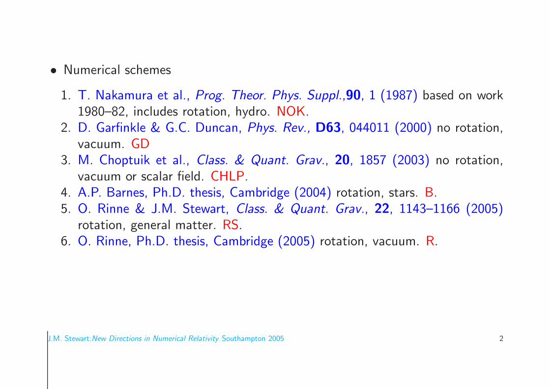
• Numerical schemes

1. T. Nakamura et al., Prog. Theor. Phys. Suppl.,90, 1 (1987) based on work1980–82, includes rotation, hydro. NOK.

2. D. Garfinkle & G.C. Duncan, Phys. Rev., D63, 044011 (2000) no rotation,vacuum. GD

3. M. Choptuik et al., Class. & Quant. Grav., 20, 1857 (2003) no rotation,vacuum or scalar field. CHLP.

4. A.P. Barnes, Ph.D. thesis, Cambridge (2004) rotation, stars. B.5. O. Rinne & J.M. Stewart, Class. & Quant. Grav., 22, 1143–1166 (2005)

rotation, general matter. RS.6. O. Rinne, Ph.D. thesis, Cambridge (2005) rotation, vacuum. R.


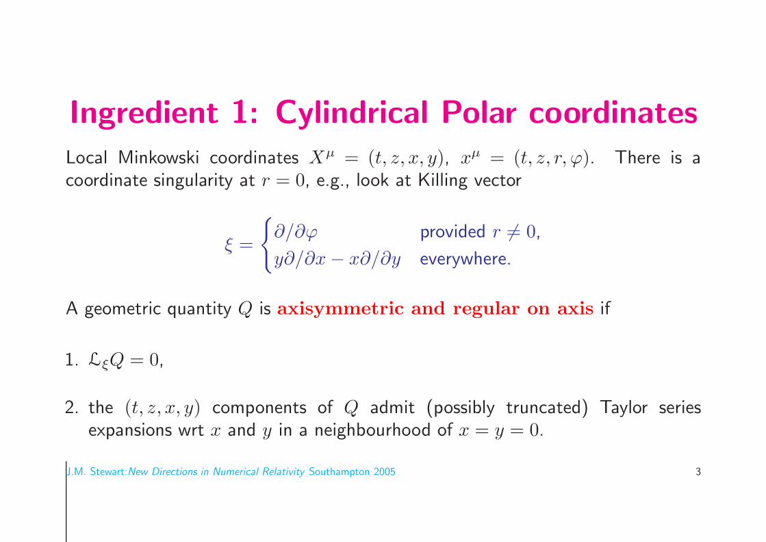
Ingredient 1: Cylindrical Polar coordinates

Local Minkowski coordinates Xµ = (t, z, x, y), xµ = (t, z, r, ϕ). There is acoordinate singularity at r = 0, e.g., look at Killing vector

ξ =

∂/∂ϕ provided r 6= 0,

y∂/∂x− x∂/∂y everywhere.

A geometric quantity Q is axisymmetric and regular on axis if

1. LξQ = 0,

2. the (t, z, x, y) components of Q admit (possibly truncated) Taylor seriesexpansions wrt x and y in a neighbourhood of x = y = 0.


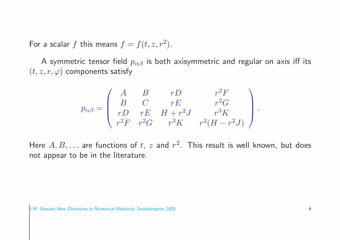
For a scalar f this means f = f(t, z, r2).

A symmetric tensor field pαβ is both axisymmetric and regular on axis iff its(t, z, r, ϕ) components satisfy

pαβ =

A B rD r2FB C rE r2GrD rE H + r2J r3Kr2F r2G r3K r2(H − r2J)

.

Here A,B, . . . are functions of t, z and r2. This result is well known, but doesnot appear to be in the literature.


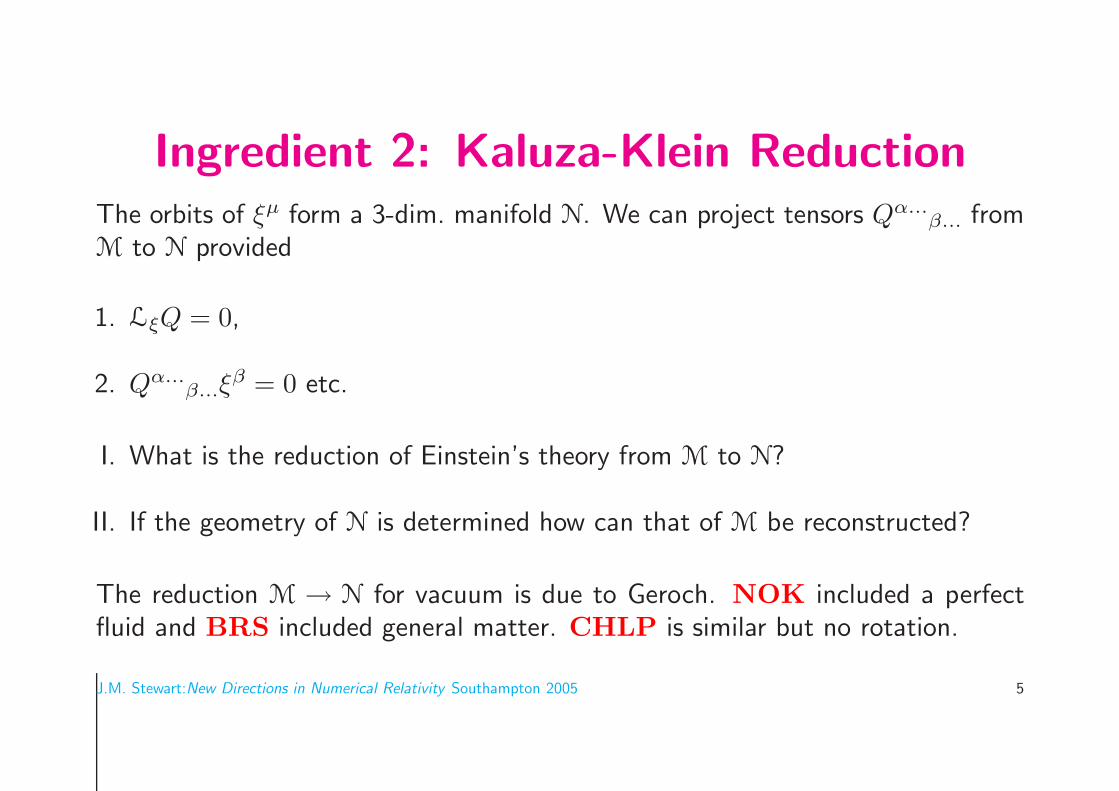
Ingredient 2: Kaluza-Klein Reduction

The orbits of ξµ form a 3-dim. manifold N. We can project tensors Qα...β... from

M to N provided

1. LξQ = 0,

2. Qα...β...ξ

β = 0 etc.

I. What is the reduction of Einstein’s theory from M to N?

II. If the geometry of N is determined how can that of M be reconstructed?

The reduction M → N for vacuum is due to Geroch. NOK included a perfectfluid and BRS included general matter. CHLP is similar but no rotation.


Geroch described the transition N → M. Difficult to implement numericallybut, fortunately, sensible physical questions in M seem to have answers in N.E.g., gravitational radiation. The leading term in Ψ4 measured wrt asymptoticNP tetrad in M can be evaluated from quantities determined in N.

N has signature ( + − −) and so we can perform an “ADM” reduction, the(2+1)+1 approach.

One novelty is that the rotation variables in N, the components of thetwist vector (curl of the Killing vector projected into N), satisfy equations whoseprincipal part is that of (axisymmetric) Maxwell equations. They couple to matterand geometry only through source terms.


Ingredient 3: Regular Variables &Equations

The first ingredient tells us the behaviour of all quantities near the axis r = 0.We redefine the dependent variables Q to be of the form

Q = f(t, z, r2) or Q = rg(t, z, r2),

so that we can impose either Neumann (∂Q/∂r = 0) or Dirichlet (Q = 0)boundary conditions at r = 0. Thus our dependent variables are manifestlyregular on axis r = 0.

We can also redefine them1, maintaining regularity, so that the new equationsare manifestly regular at the axis (no r−1, r−2, . . . factors) provided the dependentvariables satisfy the boundary conditions above.

1You need a competent computer algebra package, e.g., REDUCE, to verify this.


Flavouring: Gauge Choices

We have almost all of the ingredients to make a numerical algorithm. But weneed to make gauge and other choices. Since these are a matter of taste we callthem flavourings.

The first class of flavours comes from noting that the spatial metric HAB is2D and all 2D metrics are conformally flat so that we can choose the spatialcoordinates to set

HAB =

(

ψ4 00 ψ4

)

.

There are at least three subclasses, each favoured by different groups.

Free evolution used by GD solves the minimum number of ellipticequations. The shift vector βA is determined as the solution of gauge conditionsimplied by the choice of HAB above and its time derivative. Maximal slicing


generates an elliptic equation to determine the lapse α. Everything else isdetermined by a hyperbolic evolution system.

Although this looks very plausible we found it rather difficult to implementbecause of instabilities. If we denote the constraints by C we can derive anevolution equation for them

∂tC = FA∂AC +GC,

so that if C = 0 initially then C ≡ 0. However the matrix F r has complexeigenvalues and so this is not a hyperbolic system—the IVP for the constraints isill-posed. We can modify the slicing condition by adding an appropriate multipleof the energy constraint so as to make the above system hyperbolic. Unlike GD

we have chosen to solve elliptic equations using Multigrid techniques so as toobtain computationally efficient algorithms. However Multigrid fails for the newslicing condition because the underlying matrix becomes indefinite, even for weak


perturbations of flat spacetime.

Another subclass is constrained evolution favoured by CHLP, whereduring the evolution elliptic constraint equations are solved for α, βA and ψ. Wefound problems with the slicing and energy constraint equations. Ignoring twistand matter terms R determines the latter to be

∆ψ +K2ψp = 0 in Ω, ψ = 1 on ∂Ω,

where K2 is the square of the extrinsic curvature and p = 5. This is notlinearization stable and there is no maximum principle to imply existence anduniquess. It can be shown2 that the Dirichlet problem has at least one nontrivialweak solution provided

1 < p <n+ 2

n− 2,

2See L.C. Evans: Partial Differential Equations §8.5.2, Theorem 3.


where n is the number of space dimensions, and n = 2 here. Existence (but notuniqueness) is guaranteed, but for largeish K2 Multigrid fails for this equation(loss of diagonal dominance in the underlying matrix), as observed by B, R andCHLP for strong Brill waves.

Of course we can change the value of p to a negative one (thus guaranteeinglinearization stability) by conformally rescalingK. (This is a well-known techniquefor setting up initial data.) However R’s evolutions quickly become unstable! Hischoice of K is equivalent to that of the BSSN system which is known to havegood stability properties, and these are lost on rescaling.

Our final subclass is partially constrained evolution favoured by R. Herethe slicing condition and momentum constraints are enforced but not the energyconstraint. (There is an evolution equation for ψ.) This seemed to work allowingevolution of weak and strong Brill waves with and without twist. There is acritical amplitude for the initial data separating evolutions which disperse from


those which collapse to a black hole. However his code lacked the resolutionneeded to make quantitative statements. We need, urgently, an adaptive meshrefinement algorithm for mixed elliptic-hyperbolic systems which meets Brandt’srequirement of computational efficiency3.

As another class of flavourings one can eschew mixed elliptic-hyperbolicsystems in favour of a completely hyperbolic system. This has two advantages(i) gain control over well-posedness and outer boundary conditions, (ii) can use(Berger-Oliger) AMR.

3This is a nontrivial problem, at least to retain the O(N) efficiency of Multigrid, which is being addressed.


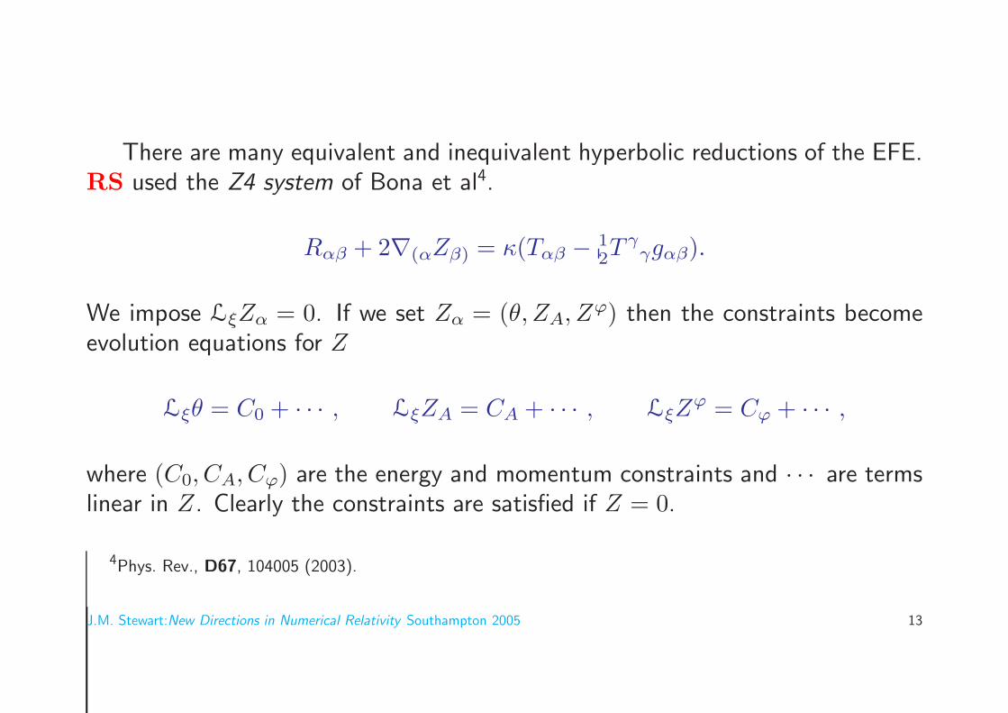
There are many equivalent and inequivalent hyperbolic reductions of the EFE.RS used the Z4 system of Bona et al4.

Rαβ + 2∇(αZβ) = κ(Tαβ − 12T

γγgαβ).

We impose LξZα = 0. If we set Zα = (θ, ZA, Zϕ) then the constraints become

evolution equations for Z

Lξθ = C0 + · · · , LξZA = CA + · · · , LξZϕ = Cϕ + · · · ,

where (C0, CA, Cϕ) are the energy and momentum constraints and · · · are termslinear in Z. Clearly the constraints are satisfied if Z = 0.

4Phys. Rev., D67, 104005 (2003).


We next introduce dynamical gauge conditions based on the generalized

harmonic gauge condition of Bona et al5. These give evolution equationsfor α and βA. One can choose the parameters to obtain a strongly hyperbolicsystem, but never a symmetric hyperbolic one.

Alternatively one can retain the evolution equation for α and require zeroshift, βA = 0. Again the system is strongly hyperbolic, and, in the special caseof harmonic gauge, the system is symmetric hyperbolic.

Using a computer algebra package one can redefine the dependent variablesso that every dependent variable and every term in every equation of our firstorder system is manifestly regular on axis. (Note that even in flat spacetime,cylindrical polar coordinates are not harmonic. We need to use the gauge sourcefunctions of Friedrich6 to ensure regularity on axis.)

5Phys. Rev., D67, 104005 (2003).6Class. & Quantum Grav., 13, 451 (1996).


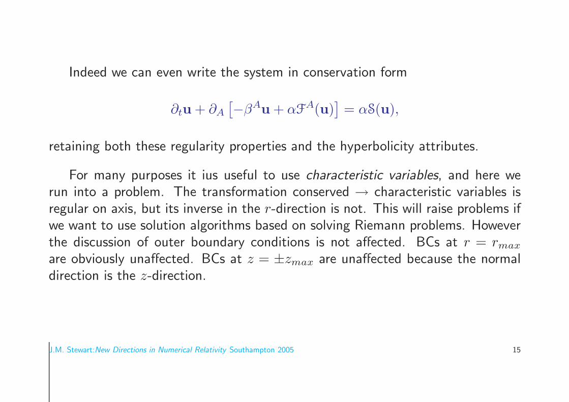
Indeed we can even write the system in conservation form

∂tu + ∂A

[

−βAu + αFA(u)

]

= αS(u),

retaining both these regularity properties and the hyperbolicity attributes.

For many purposes it ius useful to use characteristic variables, and here werun into a problem. The transformation conserved → characteristic variables isregular on axis, but its inverse in the r-direction is not. This will raise problems ifwe want to use solution algorithms based on solving Riemann problems. Howeverthe discussion of outer boundary conditions is not affected. BCs at r = rmax

are obviously unaffected. BCs at z = ±zmax are unaffected because the normaldirection is the z-direction.


Flavouring: Outer Boundary Conditions

This is a difficult problem and some experience can be gained by looking first atlinearized theory.

R looked first at dissipative BCs, and considered two such strategies

1. absorbing BCs: incoming modes are set to zero. Unfortunately the “exact”solutions of linearized theory do not obey them.

2. vanishing of Zα. These are satisfied to leading order in linearized theory butperform poorly, compared with 1, in numerical experiments.


One can do better than this.

1. Demand no incoming radiation, i.e., with a suitable Newman-Penrose tetraddefined at the outer boundaries, Ψ0 = 0. This gives two real conditions whichare satisfied to order O(r−5, z−5) in linearized theory.

2. Demand constraint preserving BCs, i.e., if we look at the subsidiary systemgoverning the evolution of the constraints, all incoming modes are set to zero.Since our linearized theory solutions satisfy the constraints to this order theysatisfy this condition.

3. Demand gauge preserving BCs, i.e., do the same as item 2 but for the evolutionsystem for α and βA. Ditto.


This gives nine conditions at each boundary, or seven for zero shift. Inaxisymmetry this is precisely the number required. The normal derivatives of theincoming modes are specified in terms of the tangential derivatives and sourceterms. R has checked them against linearized theory. Using GKS theory he haschecked a necessary condition for the well-posedness of the IBVP in the highfrequency limit.


Let me close with some very preliminary simulations carried out by R. R’scurrent evolutions are of Brill waves with twist, and the end product of a lowamplitude subcritical evolution will be flat spacetime. However the final lineelement is flat but not Minkowskian! The variable es(t, z, r) measures the ratioof circumference-radius to coordinate-radius and is zero in Minkowski spacetime.Note that the r = 0 axis (left edge) is totally stable and there is minimal reflectionfrom the far-too-close outer boundaries. s

Alcubierre has suggested that a dynamically evolved lapse can produce “gaugeshocks”, chart discontinuities, which render the subsequent evolution useless. Thesecond movie is a plot of α,r/α as a function of r and z as t increases. The boxesshow the extent of the AMR subgrids. Although the function looks “spiky” itisn’t! The still shows α,r/α at a fixed time on the finest AMR-generated subgrid.Ar, Arcloseup


The third movie shows Bϕ evolving. (The twist variables Er, Ez and Bϕ

obey Maxwell equations.) Bϕ


Conclusions

• Axisymmetric evolutions which remain regular on axis are feasible, and thereare no constraints on the algorithms to be used.

• It’s essential to be aware of the underlying mathematics, existence, uniqueness,stability etc.

• A competent computer algebra package is very useful.

• AMR is no longer a luxury; consider e.g., the “gauge shock”.

• Remember Brandt’s dictum: concentrate the effort where the physics isinteresting.


Date post:	16-Aug-2018
Category:	Documents
Upload:	phungthuy
View:	223 times
Download:	0 times

Axisymmetry in Numerical Relativitycjg/satellite/stewart.pdf · Axisymmetry in Numerical Relativity...

Documents