48
en CI) ..., ( 0 ..., en E . ' . . :::J C" W CI) - 0 ::I: (.) ( 0 - CO L. Qj t '" u c 0 "0 c L. '" CO ::.: E 0 t: l? t: C5 o \:: C5 '" '" ~ 1 5 .... ";:: .;;
| Date post: | 08-Apr-2018 |
| Category: |
Documents |
| Upload: | knarfrotcod |
| View: | 221 times |
| Download: | 0 times |
8/7/2019 b carter - equilibrium states of black holes
http://slidepdf.com/reader/full/b-carter-equilibrium-states-of-black-holes 1/48
en
CI)
..., (0..., en
E:::J.'
.
.:::J
C"W
CI)
-0
::I:
(. )
(0
-CO
L.
Qj
t
'"u
c0
"0
c
L.'"CO
::.:E0t:
l?
t:C5
o\::
q;CXl
C5
'" '"~ 1 5 ....
";::
.;;

8/7/2019 b carter - equilibrium states of black holes
http://slidepdf.com/reader/full/b-carter-equilibrium-states-of-black-holes 2/48
Contents
Part I Analytic and Geometric Properties of the Kerr Solutions
I Introduction 61
2 Spheres and Pseudo- Spheres 62
3 Derivation of the Spherical Vacuum Solutions 68
4 Maximal Extensions of the Spherical Solutions 74
5 Derivation of the Kerr Solu tion and its Generalizations 89
6 Maximal Extensions of the Generalized Kerr Solutions 103
7 The Domains of Outer Communication 112
8 Integration of the Geodesic Equations . 117
Part II General Theory of Stationary Black Hole States
I Introduction 125
2 The Domain of Outer Communications and the Global Horizon. 133
3 Axisymmetry and the Canonical Killing Vectors 136
4 Ergosurfaces, Rotosurfaces and the Horizon 140
5 Properties of Killing Horizons 146
6 Stationarity, Staticity, and the Hawking-Lichnerowicz Theorem 151
7 Stationary-Axisymmetry, Circularity , and the Papapetrou Theorem 159
8 The Four Laws of Black Hole Mechanics 166
9 Generalized Smarr Formula and the General Mass Variation Formula 177
10 Boundary Conditions for the Vacuum Black Hole Problem 185
II Differential Equation Systems for the Vacuum Black Hole Problem 197
12 The Pure Vacuum No-Hair Theorem 205
13 Unsolved Problems 210
59
8/7/2019 b carter - equilibrium states of black holes
http://slidepdf.com/reader/full/b-carter-equilibrium-states-of-black-holes 3/48
PART I Analytic and Geometric Properties of the
Kerr Solutions
Introduction
The Kerr solu tions (Kerr 1963) and their electromagne tic generalizations(Newman et al. 1965) form a 4-parameter family of asymptotically flat solu tions
of the source-free Einstein-Maxwell equations, the parameters being most con
veniently taken to be the asymptotically defined mass M, electric charge Q, and
magnetic monopole charge P, together with a rotation parameter a, which is such
that (in u n i t ~ of the form we shall use throughout , where the speed of light c and
Newton's constant G are set equal to unity) the asymptotically defined angular
momen tum J is given by
J=Ma
The parameters may range over all real values subject to the restriction
M2 ;;;;. a2 + p 2 + Q2
which must be satisfied if the solution is to represent the exterior to a hole rather
than naked singularity. It turns out (Carter 1968a) that the solutions all have the
same gyromagnetic ratios -as those predicted by the simple Dirac theory of the
electron, as the asymptotic magnetic and electric dipole moments cannot be
specified independently of the angular momentum but are given, in terms of the
same rotation parameter, as Qa and Pa respectively.
The solutions are all geometrically unaltered by variations of P and Q provided
that the sum p2 + Q2 remains constant, and since it is in any case widely believed
that magnetic monopoles do no t exist in nature, attention in most studies is re
stricted to the 3-parameter subfamily in which P is zero. This 3-parameter sub
family, and specially the 2-parameter pure vacuum subfamily in which Q is also
zero, has come recently to be regarded as being at least potentially of great
astrophYSical interest, since the Kerr solutions do no t merely represent the only
known stationary source-free black hole exterior solu tions: they are also widely
believed (for reasons which will be presented in Part IT of this course) to be the
only poss ible such solutions.
We shall devote the whole of Part I of the present lecture course to the
derivation and geometric investigation of these Kerr solutions. In a strictly logical
approach, Part IT of this course (which will consist of a general examination of
stationary black hole states with or without external sources) should come first,
but it is probably advisable for a reader who is not already familiar with the sub
ject to start with Part since the significance of the reasoning to be presented in
Part IT will be more easily appreciated if one has in mind the concrete examples
61
8/7/2019 b carter - equilibrium states of black holes
http://slidepdf.com/reader/full/b-carter-equilibrium-states-of-black-holes 4/48
6362 B. CARTER
described in Part 1. For the same reason many readers may find it easier to
appreciate the accompanying lecture course of Hawking if they have first become
familiar with the examples described here, although only the final stages of
Hawking's course actually depend on the results presented here, the bulk of it
being logically antecedent to both Part II and Part I of the present course. This
present lecture course is intended to serve both logically and pedagogically as
an in troduction to the immediately following course of Bardeen and hence also
(but less directly) to the subsequent courses in this volume.
2 Spheres and Pseudo-Spheres
A space time manifold vi i is said to be spherically symmetric if it is invariant
under an action of the rotation group SO (3 ) whose surfaces of transitivity are
2-dimensional. The metric on anyone of these 2-surfaces must have the form
d s ~ =r2 (df)2 + sin2f)d<p2) (2.1 )
in terms of a suitably chosen azimuthal co-ordinate f) running from 0 to 11", and a
periodic ignorable co-ordinate <p defined modulo 211", where the scale factor r is
the radius of curvature of the 2-sphere. In what follows we shall frequently fmd
it convenient to use the equivalent alternative form
dl12 }d s ~ = r 2 1 - 11 2+ (l_112)d<p2 (2.2){
expressed in terms the customary alternative azimuthal co-ordinate
11 =cos f) (2.3 )
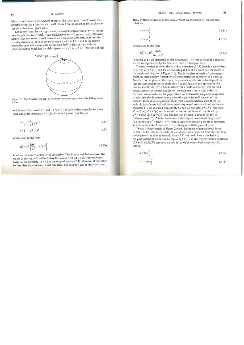
running from -1 to +l. See Figure 2.1.
A space-time mani fold vi i is said to be pseudo-spherically symmetric if it is
invariant under an action of the 3-dimensional Lorentz group whose surfaces of
transitivity are timelikeand 2-dimensional. The metric on one of these 2-surfaces
can be expressed in a form analogous to (2) as
2 2 {dx2
2 2}ds x =-s - -2 - (1 - x )d t (2.4 )I- xwhere s is the radius of curvature and where the co-ordinate t is ignorable.
The two simple and familiar metric forms d s ~ and d s ~ illustrate a feature
which will crop up repeatedly in the present course, that is to say they both have
removable co-ordinate Singularities. The spherical form (2.2) is obviously Singular
at 11 = ± I; moreover we cannot remove this singularity simply by returning to the
form (2.1) in which the infinity is eliminated only at the price of introducing an
equally undesirable vanishing determinant which will of course lead to an infinity
in the inverse metric tensor. We can cure the singularity and show explicitly that
the space is well behaved at the poles (as we know it must be by the homogeneity)
BLACK HOLE EQUILIBRIUM STATES
1a 1b
8
t
(/)
x
o
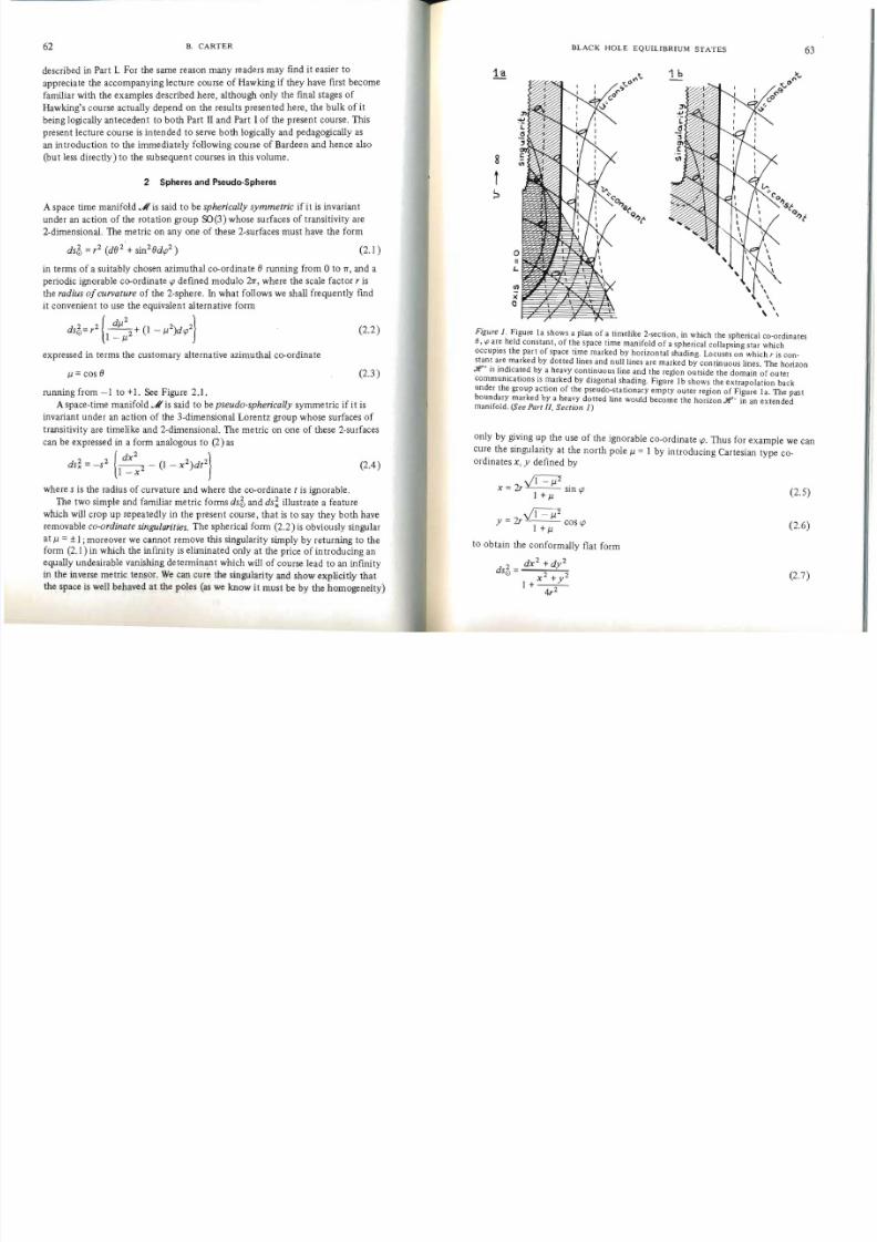
Figure 1. Figure la shows a plan of a timelike 2-section, in which the spherical co-ordinates
e, <p are held constan t, of the space time manifold of a spherical collapsing star which
occupies the part of space time marked by horizontal shading. Locuses on which r is con
stant are marked by dotted lines and null lines are marked by continuous lines. The horizon£+ is indicated by a heavy continuous line and the region outside the domain of outer
communications is marked by diagonal shading. Figure lb shows the extrapolation back
under the group action of the pseudo-stationary empty outer region of Figure lao The pa'st
boundary marked by a heavy dotted line would become the horizon£ - in an extendedmanifold. (See Part II, Section 1)
only by giving up the use of the ignorable co-ordinate <p. Thus for example we can
cure the singulari ty at the north pole 11 = I by introducing Cartesian type co
ordinates x , y defined by
VI - 112x = 2r sin <p (2.5)1 + 11
Y = 2r cos <p (2.6)1+11
to obtain the conformally flat form
dx2 + dy2
d s ~ = 2 2 (2.7)X +y1+--
4r2
8/7/2019 b carter - equilibrium states of black holes
http://slidepdf.com/reader/full/b-carter-equilibrium-states-of-black-holes 5/48
65B. CARTER64
which is well behaved everywhere except at the south pole. It is of course im
possible to obtain a form which is well behaved on the whole of the 2-sphere at
the same time (see Figure 2.1.).Let us now consider the algebraically analogous singularities at x == ± 1 in the
pseudo-spherical metric d s ~ . These singularities are of a geometrically different
nature since the metric is well behaved with the same signature, on both sides of
the singularities i.e. both in the static regions withIx
I> I and in the regionswhere the ignorable co-ordinate is spacelike Ix 1<1. (I n contrast with the
spherical metric which has the right signature only for If-L I< 1.) We can link the
Norl;.h Pole ).J. =-1
--."..,/,
-i.l,.: .O __ .....
,;/
-------_ ....
Figure 2.1. The 2-sphere. The light dotted lines represent trajectories of the Killing vector
afa",.
well behaved domains x> I and - I < x < I by a co-ordinate patch extending
right across the divisions x == ± I , by introducing new co-ordinates
T== -x t (2.8)I I_x 2 Ite
t (2.9)A== II - x2
e
which leads to the form
2(2.10)ds2 == s2 (cfl.... _ A
2dT2}x A2
In which the new co-ordinate T is ignoreable. This form is well behaved over the
whole of the region A> 0 including the loci AT == ± I which correspond respec
tively to the divisions -x == ±l in the original system (2.4). Moreover it can easily
be seen that these loci are in fact null lines. The situation can be visualized most
BLACK HOLE EQUILIBRIUM STATES
easily in terms of null-co-ordinates u , v which we introduce by the defining
relations
IU==T+- (2.11 )
A
I V==T- - (2.12)
A
which leads to the form
d s ~ == _ 4s2 dudv (2.13)(u - v)2
(whose u and v are restricted by the condi tion u - v > 0) in which the divisions
x == ±I are represen ted by the lines u == 0 and v == 0 respectively.
The relationship between the co-ordinate patches (2.13) (which is equivalent
to (2.10) with A> 0) and the co-ordinate pat ches of the form (2.7) is shown in
the conformal diagram of Figure 2.2a. This is the first example of a technique,
which we shall emp loy frequen tly, of represen ting t he geome try of a timelike
2·surface on the plane of the paper, in a manner which takes advantage of the
fact that any such metric is conformly flat and thus can be expressed in the
canonical null form ds 2 == Cdudv where C is a conformal factor. The method
consists simply of identifying the null co-ordinates u and v with ordinary
Cartesian co-ordina tes on the paper whi ch conven tionally are placed diagonally
so that timelike di rections lie in a cone of angles within 45 degrees of the
vertical. There is nothing unique about such a representation since there is a
wide choice of canonical null form preserving transformations in which the co
ordinates u, v are replaced respectively by new co-ordinates u*, v* of the form
u* == u*(u), v* == v*(v) and in which the conformal factor C is replaced by
C* == C(du* jdu )(dv*jdv) . This freedom can be used to arrange for the co
ordinate range u* , v* to be finite even if the original co-ordinate range is not
(e.g. by taking u* == tanh u, v* = tanh v) thereby making it possible to represent
an infini te timelike 2-manifold in its entirety on a finite piece of paper.
The co-ordinate patch of Figure 2a wi th the spacially homogeneous form
(2.10) is in fact still incomplete , as would have been expected from the fact that
starting from the time symmetric form (2.4) one could have extended into
the past instead of the future by replacing t by - t in the transformation equations
(2.8) and (2.9). We can obtain a new form which covers both extensions by
setting
u == tan 2:u (2.14)
vv = - co t - (2.15)
2

8/7/2019 b carter - equilibrium states of black holes
http://slidepdf.com/reader/full/b-carter-equilibrium-states-of-black-holes 6/48
66
67
B. CARTER
which leads to the new null form
(2.16)f U - VId s ~ =_ s2 \1 + tan
2dUdV
In terms of these co-ordinates (which can both range from -00 to 00 subject to
the restriction -n < U - V < n) the entire co-ordinate range of u and v subject
to u + v < 0, i.e. the entire range of A, 'T subject to A> 0, is covered by the range
\
\
(.0.
,0" 1
8,... ' / ~ '
(,. A'".' 1 f" , . . ' ~ /II t<.
0 o , If
I &,
I" IH
II
(.0. II
// - - ~ ~ " (f'-
, f
- .... ... ', ' \II" _-_ , . ,\0" I 1&
+\I
,t<\c? ", -----0" \, ... ,/ I I
\,""
,\
\
\
\
\
\
// ' , __ / ' 1/
..)-" " ,.., / 8 \ ,"
... \
\
\' \ \ ><
\1 ~ ' ' \"o 0 ~ " , , \ \"/ " ,\ 8 \
...:r )" , \
A
,cf'I
..)
\
\
,\
II
I
I
2.2a 2.2b
Figure 2.2 Conformal diagram of the 2-dimensional pseudo-sphere . In Figure 2a the light
dotted lines represent trajectories of the Killing vector a/at and the heavy lines representthe corresponding non-degenerate Killing horizons. In the extended diagram of Figure 2bthe light dotted lines represent trajectories of the Killing vector a/aT, and the double lines
represent the corresponding degenerate Killing horizons.
0< V < 2n, and -n < U< n . The situation is illustrated in Figure 2b. The mani
fold in this figure is geodesically complete and hence maximal in the sense that
no further extension can be made. The null form (2.16) covering this maximal
extension can be converted to an equivalent static form by introducing co-ordinates
X, T defined by
U - VX= tan -2- (2 .17)
BLACK HOLE EQUILIBRIUM STATES
T= U+ V(2 .18)
2
which gives the maximally extended static form
dX2 }ds2 = +s2 --_ (1 + X2 )dT2 (2.19)
x {1+ X2
in which X and Tcan range from _00 to 00 without restriction.Looking back from the vantage point of this complete manifold we can see
clearly what has been happening. The timelike Killing vector whose trajectories
are the static curves x = constant, Ix I> 0 in the system (2.4), becomes null on
the surfaces on which U or V are multiples of n, these surfaces representing past
and future event horizons for observers who are fixed in that x remains constant
relative to this system. [The past and future event horizon (cf. Rindler 1966) of
an observer being respectively the boundary of the past of his worldline, i.e. the
set of events he will ultimately be able to know of , and the boundary of the
future of his world line Le. of the set of events which he could in principle have
influenced.] Thus for the Killing vector whose trajectories are the static lines
x =constant, I x I> 0 in the system (2.4), the corresponding event horizons are
the lines on which U and V are multiples of n. In the extension (2.10) in which
the ignorable co-ordinate t has been sacrificed, there is a new manifest symmetry
generated by the Killing vector whose trajectories are the lines A=constant, and
for the corresponding static observers the event horizons coincide with alternate
horizons of the previous set, specifically the lines on which U + n and V are
mUltiples of 2n. In the maximal extension in which the ignorable co-ordinate T
has in its turn been replaced by T, there is a third non-equivalent Killing vector
field, whose static trajectories are the lines X = constant, and in this case the '
corresponding observers have no event horizons.
There is a fairly close analogy between the removable co-ordinate singularities
associated with rotation axes, as exemplified by the case of the ordinary 2-sphere
discussed earlier, and the removable co-ordinate singularities associated with
Killing horizons. Both arise from the inevi table bad behaviour of an ignorable
co-ordinate which is used to make manifest symmetry group action generated bya Killing vector. The former case arises in the case Of a spacelike Killing vector
generating a rotation group action when it becomes zero on a rotation axis, while the
latter arises in the case of a static Killing vector (and also under appropriate
conditions as we shall see later a stationary Killing vector) when it becomes null
on a Killing horizon. Killing horizons can be classified as degenerate or non
degenerate according to whether the gradient of the square of the Killing vector
is zero or not. In the case of a non-degenerate Killing horizon (as exemplified by
the horizons on which the Killing vecto r whose trajectories are x =constant) the
relevant Killing vector must change from being time like on one side to being
spacelike on the other. In the case of a degenerate Killing horizon, the relevant
8/7/2019 b carter - equilibrium states of black holes
http://slidepdf.com/reader/full/b-carter-equilibrium-states-of-black-holes 7/48
68
69B. CARTER
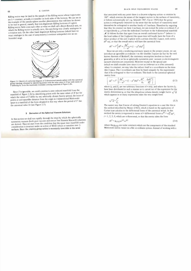
Killing vector may be (and in the sample of the Killing vector whose trajectories
are A= constant, actually is) timelike on both sides of the horizon. We can see in
the example of the pseudo-sphere another phenomenon that will later be shown
to be true in general , namely that non-degenerate Killing horizons of a given
Killing vector field crosS each other at what we shall call a Boyer-Kruskal axis, on
which the Killing vector is actually zero, this axis being very closely analogous to
a rotation axis. On the other hand degenerate Killing horizons (which have no
exact analogue in the case ofaxisymmetry ) continue unimpeded over an un
bounded range.
).. or 00
, , -- - - - " , " ,... /
... /
... "... ," ,,,,
" I/ ' , ,0 ,"
-r ' ', , , ' I
'Jt' ,J'..... ,",.,;/
" / " - ' ", : ~ " " , , , , _ _ _ ;>..=_CJIO
Figure 2.3. Sketch of conformal diagram of 2-dimensional pseudo-sphere with the canonicalglobal topology obtained by identifying points with the same value of X bu t with values of
T differing by 21T in the maximally extended covering manifold of Figure 2.2b.
Since T is ignorable , we could construct a new reduced manifold from the
manifold of Figure 2.2b by identifying points with the same values of X but for
which the values of T differ by any arbitrarily chosen fixed p period; the locus of
points at unit spacelike distance from the origin in 3-dimensional Minkowski
space is a manifold of the form obtained in this way where the period of T has
the canonical value 21T (see Figure 2.3).
Derivation of the Spherical Vacuum Solutions
In this section we shall run rapidly through the steps by which the spherically
symmetric vacuum (both pure vacuum and source free Einstein Maxwell) solutions
are derived. Thus we start from the condition that the space time manifold under
consideration is invariant under an action of SO (3) which is transitive over 2
surfaces. Since the rotation group action is necessarily invertible in the sense
BLACK HOLE EQUILIBRIUM STATES
that associated with any point there is a discrete subgroup action-a rotation by
1800
-which reverses th e senses of the tangent vectors to the surfaces of transitivity ,
it follows automatically (cf. e.g. Schmidt 1967, Career 1969) that the group
action is orthogonally transitive in the sense that the surfaces of transitivity must
themselves be orthogonal to another family of 2-surfaces. Therefore by requiring
that they be constant on these 2-surfaces, we can extend the polar co-ordinate e, <{!
or equivalently 11 , <{! from the individual 2-surfaces to the 4-dimensional manifold
..JI. It follows further that apart from an overall conformal factor r2 (where r isthe local radius of the 2-spheres) the space-time will locally have the form of a
direct product of the unit 2-sphere with a certain time-like 2-space, with metric
dl 2 say, so that the overall metric will have the canonical form
2 2ds = r2 {d1 + 1~ : 2 + (1 - 112)d<{!2} .
Since we are only c ::msidering stationary spaces in the present course, we can
introduce an ignorable co-ordinate t on the timelike 2-spaces (in fact by the well
known theorem of Birkhoff, the stat ionary assumption involves no loss of
generality at all in so far as spherically symmetric pure vacuum or electromagnetic
vacuum solutions are concerned). Moreover except in the special case
(which we shall consider later since it is not as irrelevant as is often assumed)
when r is constant, we may take the radius r itself as a co-ordinate on the timelike 2-space. The t co-ordinate can then be fixed uniquely by the requirement
that it be orthogonal to the r co-ordinate. This leads to the c a n o n i c ~ l spherical
metric form
2dl12 r2
ds 2 = r2 1-112+ (1_112)d<{!2 +dr _ L:::. dt } (3.2)
{ . L:::. r Z2r
whe re L:::.r and Z r are two arbitrary functions of r only, and where the factor s L:::. r
have been distributed in such a manner as to cancel ou t of the expression for the
metric determinant g, so that the ubiquitous volume density weight factor
which appears in so many expressions takes the very simple form
4r
-Fi=- (3.3)Zr
The easiest way that I know of solving Einstein's equations in a case like this is
the method described by Misner (1 963) , which is based on the application of
Cart an type calculus to the differential forms of the canonical tetrad. In this
method the metric is expre ssed in terms of 4 differential forms w(i) = w ~ ' ) dx G ,
i = 1,2,3,0, which are orthonormal, so that the metric takes the form
ds 2 = g(i) ( j)w (i ) w (j) (3.4 )
where the g(i)v1 are scalar constants which are the components of the standard
Minkowski metric tensor in a flat co-ordinate system. Instead of working with a
3

8/7/2019 b carter - equilibrium states of black holes
http://slidepdf.com/reader/full/b-carter-equilibrium-states-of-black-holes 8/48
7071
B. CARTER
large number of Christofel symbols one works with what will (specially if the
original metric form is fairly simple) be a comparatively small number of
connection forms, -y(i)(j) = -y(i)(j) dxa defined (but no t in practice computed) by
the equations
di)a;b = -y(i) (j)bWU)a (3.5)
These forms will au tomatically be symmetric in the sense that if the labelling
indices are lowered by contractions with the Minkowski scalors i.e. setting-Y(i)U) = g(i)(k) 'Y(k){j) , then we have they will satisfy
(3.6)-y (i ) (j ) = -yU)( i)
Moreover the antisymmetrized part of the equation (3.5) can be expressed in
terms of Cartan form language as
ddi) = _-y(i)(j) /\ wU) (3.7)
and it can easily be seen that the two expression (3 .6) and (3 .7) together (which
can easily be worked out without using covariant differentiation) can be used to
determine the forms -y(i)U) instead of the computationally more awkward defining
relation (3.4). Furthermore the tetrad componen ts R (i )U)(k )(1) of the Riemann
tensor can also be read out without the use of covariant differentiation from
the expression
8(i)( j) = 1R ( i)( j)(k)(l)w(k) /\ w(1) (3.8)
a bwhere the curvature two· forms 8(i) (j ) =e (i) (j)ab dx /\ dx are given (as can easily
be checke? by differentiating (1) and using the defining relationW(l)a(b;cJ =
1RabcdW(I)a bv
e(i) (j ) = dii)U) + -y(i)(k) /\ -y(k)(j ) (3.9)
The tetrad components of the Ricci tensor are obtained simply by contracting
R(i}( j ) =R(k\i )(j )(k) (3.10)
and if required the co-ordinate form is given by(3.11 )
Rab =R( i)U)W(i)aWU)b.
In the present case the obvious tetrad of forms consists of
w( l ) = _r_ d r
A(2) _ r dJ1
(3.l2)w
w ( 3 ) = r ~ d < . p dO ) = rvz;;.d t
Zr
BLACK HOLE EQUILIBRIUM STATES
and a straightforward calculation on the lines described above shows that the
only solution of the pure Einstein vacuum equations
R;j = 0 (3.13)
are given (after use of co·ordinate scale change freedom to achieve a standard
normalization·) by
Zr = r2 (3.14)
Do =r2 - 2J',1r (3.15)r
where M is a constant . The corresponding values of the curvature forms may be
tabulated as
M Me(1) - - w(l) /\ d 2 ) e(3)(O) = - r3 w(3) /\ dO )
(2) - - r3
M Me(3) = - w(l) /\ d 3) e(3)( = 2 - d 2) /\ w(3) (3.16)(I ) r3 2) r3
e(O)(1) = 2 w( l ) /\ w(O) e(O) =-M w(2) /\ ,../0)(2) r3r
The comparative conciseness of this array, from which, if desired, all 20 of the
ordinary Riemann tensor components can be read out, shows clearly the advantage
of the Cartan formulation . If one is interested in the Petrof classification, it can
be seen directly from the above array that the tetrad w(i) is in fact a canonical
tetrad and that the Riemann tensor, which in the vacuum case is the same as the
Weyl conformal tensor, is of type D. (See Pirani 1964, 1962; Ehlers and Kund t 1%2.
The familiar Schwarzschild metric itself is given explicitly by
dr2 dJ12 2 } ((2 - 2J',1r) 2ds
2= r2
{2 +--2 - (1 - J1 )d<.p2 - 2 d t (3.17)
r - 2J',1r I - J1 r
To obtain the electromagnetic vacuum solutions we must first find .the most
general forms of the electromagneti c field consistent with spherical symmetry.We start from the well known fact that there are no spherically symmetric vector
fields on the 2·sphere , and only one unique (apart from a scale factor) spherically
symmetric 2-form on the 2·sphere, which takes a very simple fonn in tenns of
the co-ordinate system (2.2), namely dJ1/\ d<.p. Since any cross components of
the Maxwell field between directions orthogonal to and in the 2·spheres of
transitivity would define vector fields in the surfaces of transitivity it follows
that the most general spherical Maxwell field is a linear combination with co
efficients depending only on r, of dr /\ d t and dJ1/\ d<.p, and hence can be expressed
in terms of the canonical tetrad in the form
F= 2E w( l ) /\ w(O) + 2B w(2) /\ w(3)r r (3.18)

8/7/2019 b carter - equilibrium states of black holes
http://slidepdf.com/reader/full/b-carter-equilibrium-states-of-black-holes 9/48
7273B. CARTER
where E, and B, are functions of r only. The dual field form *F is then given
simply by
*F= 2B,w(l) /\ w(O) + 2E,w(2) /\ W(3) (3.19)
and in terms of these expressions the source free Maxwell equations simply take
the form dF = 0, d *F = 0 and thus they too can be worked ou t by the Cartan
method without recourse to covariant differentiation. The electromagnetic
energy tensor will be given by
8rrTab = (E; +B; ) O ) w b O ) + w13)wb3) + w ~ 2 ) w b 2 ) - w ~ l ) w b l ) } (3)0)
and hence the Einstein-Maxwell equa tions
(3.21 )Rab = 8rrTab
can easily be worked out with the Ricci tensor evaluated in the way described
above.
The solu tions are given by
Q P (3.22)E, =2 B '=2
r r
(where Q and P are constants which correspond respectively to elect ric and
magnetic monopole charges) with
(3.23)z, =r2
t:., = r2 _ 2Mr + Q2 + p2 (3.24)
In presenting the information giving the curvature, it is worthwhile to make a
distinction now between the Riemann tensor, and the Weyl conformal tensor
since the Ricci tensor which may be read out by substituting (3.20)in (3.21)and
using (3.22), is no longer zero. The Weyl forms D,(i)(j) =D,(i)(j)ab w ~ i ) w ~ ) defined in terms of the tetrad componen ts e i) (j)(k) (I ) by
D,(i)(j) = 1 C ( i ~ ( j ) ( k ) ( l ) W ( k ) /\ w(1) (3.25)
are related to the curvature forms e(i)(j) by
D,(i)(i) =e(i)(j) + R[( i)(k)w(j) l /\ w(k) + iRw( i ) /\ w(j ) (3.26)
where R is the Ricci scalar (which is of course zero in the present case). The Weyl
form may be tabulated as
Mr _ Q2 _ p2 '(
I) Mr - Q2 - p2 (I) (2) D,(O) (3) =-. r w(3) /\ w(O)D, (2) =-, w /\ w 4
r
(3) Mr - Q2 _ p2D,(3) _ Mr - Q2 - p2 (3) /\ (I ) D, (2) =2, w(3) /\ w(3) (3.27)
(I ) - r4 w wr
D,(O) _ Mr - Q2 - p2 (0) /\ W(2)D,(O)(I) = 2 Mr - - p2 w(O) /\ w( l) (2)-, w
r
BLACK HOLE EQUILIBRIUM STATES
Again the form of this array makes it immediately clear to a connoisseur that
the solu tion is of Petrov type D. The explicit form of the electromagnetic field is
2Q 'F =- 2 - dr /\ dt + 2P df.1 /\ d<{! (3.28)
r
which may be derived via the relation
F= 2dA (3 .29 )
from a vector potential A given by
A =Q. dt - Pf.1 d<{! (3.30)r
The explicit form of the metric itself is
dr2 df.12 } r2 _ 2Mr + Q2 + p22ds =r2 r2_2Mr+Q2+p2+1 _ f.12+(l-f.12)d<{!2 - r2 dt[
(3.3 I)
this being the solution of Riessner and Nordstrom , which of course includes the
Schwarzschild solution in the limit when Q and P are set equal to zero.
Our search for spherical solutions is not quite complete at this point because by
working with the spherical radius r as a co-ordinate, we have excluded the special
case where r is a constant. Of COurse a solution with this property cannot be
asymptotically flat, unlike the solutions which we have obtained so far, and there
fore it might be thought not to have much physical interest. However as we shall
see in the next section, it is impossible to have a full understanding of the global
structures of the solutions we have obtained so far , without considering this
special case, which arises naturally in a certain physically interesting limit.
To deal with this special case we must alter the canonical metric form (3.2)
by replacing the co-ordinate r by a new co·ordinate, 'A say , except in the con
f0,mal factor r2 ou tside the large brackets which remains formally as before, and
IS now to be held cons tan t.
Using the same methods as before, we find that there are no pure vacuum
solutions of this form, bu t that there do exist source free electromagnetic
solu tions, which can be expressed as follows: The electromagnetic field takes
the form
F = 2Q d'A /\ d t + 2P df.1 /\ d<{! (3.32)
which can be derived from a vector potential
A =Q'A dt - Pf.1 d<{! (3.33)
and the metric is given by
d'A2 d2 }ds2 = (Q2 +p2) -2 + + (I _ f.12)d<{! _ 'A2 dt 2
(3.34){ 'A I - f.1
8/7/2019 b carter - equilibrium states of black holes
http://slidepdf.com/reader/full/b-carter-equilibrium-states-of-black-holes 10/48
75B. CARTER74
This is the solu tion of Robinson and Bertotti. This metric is in fact almost as
symmetric as possible, since it can easily be seen that it is the direct product of
a 2-sphere whose radius is the square root of Q2 + p2 with a pseudo sphere (c f
the form (2.10)) of the same radius. Its maximal symmetry group therefore has
not four parameters as in the previous solutions (three for sphericity and one for
stationarity) but six.
4 Maximal Extens ions of the Spherical Solutions
It is relatively easy to analyse the global structures of the solutions which we
have just derived, since, as indicated by (3.1), all of them are equivalent, modulo
a conformal factor ,2 , to the direct product of a 2-sphere with a timelike 2-surface.
Thus the problem boils down to an analysis of the timelike 2-surfaces with metric
dsl == ,2dl2
, whose structures can be represented by the simple conformal
diagrams whose use was described in section (1).The simplest case is of course Simply flat space to which the Schwarzschild
form (3.17) reduces when the mass parameter is set equal to zero. The
corresponding timelike 2-dimensional metric is simply d,2 - dt2 with the
restriction 1T > 0, which, via the transformation u == , - t, v == , + t, is equivalent
to the flat null form 2 du dv, with the restriction u + v > O. The corresponding
conformal diagram is given in Figure 4.1, in which the null boundaries.f+ and§- which playa key role in the Penrose definition of asymptotic flatness are
marked. To qualify as asymptotically flat in the Penrose sense-which he refers
to as the condition of weak asymptotic simplicity-a spacetime manifold must
be conformally equivalent to an extended manifold-with-boundary with well
behaved null boundary horizons j+ and j- isomorphic to those of flat space.
(Asymptotic flatness is discussed in more detail in the accompanying course of
Hawking.)
The Schwarzschild soluti on is of course asymptotically flat in this sense, and
indeed when M is negative the conformal diagram of the metric
,2 d,2 ,2 _ 2M,dSI == 2 - 2 dt
2. (4.1)
, - 2M, ,
is topologically iden tical to the flat space diagram of Figure 4 . 1, although there
is the important geometric difference that whereas in the former case the
boundary' == 0 represented only a trivial co-ordinate degeneracy at the spherical
centre, in the latter case, as can be seen from a glance at the array (3.l6) it rep
resents geometric singularity of the Riemann tensor. In the physically more
interesting case where M is positive the Schwarzschild conformal diagram still
agrees with the flat space diagram for large values of " in accordance with the
Pe,nrose criterion, but it has an entirely different behaviour going in the other
direction due to the fact that the metric form (3 .17) becomes singular not only
a t, == 0 but also a t , == 2M. The fact that the Riemann components, as exhibited
in the array (3 .16), are perfectly well behaved there suggests that this may not
BLACK HOLE EQUILIBRIUM STATES
be a true geometric singularity !Jut merely a removable co-ordinate singularity of
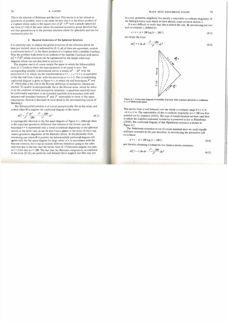
the Killing horizon type which we have already corne across in section 2 It is no t difficult to verify that this is indeed the case. By introducing just one
null co-ordinate v, defmed by
v == t + {, + 2M log I, - 2M I} (4.2)
we obtain the form
2 ,2 - 2M, 2ds1 == 2 dv d, - dv, (4.3)
+Pj+
II
II
IJI
\
\
I ,I,I
I
I /I
I
/
I
I
I /, I
, I
It.
Figure 4.1. Conformal diagram of timelike 2-section with constant spherical c(H)rdinates O;«J of Minkowski space.
This metric form is well behaved over the whole co-ordinate range 0 < , < 00
- - 00 < V < 00 . The removability of the co-ordinate singularity a t ' == 2M was first
pOinted out by l.emaitre (1933). The type of transformation we have used here
in which the manifest stationary symmetry is preserved is due to Finkelstein(I958). The conformal diagram of this Fipkelstein extension is shown inFigure 4.2 .
The Fmkelstein extension is no t of cOlfrse maximal since we could equally
well have extended in the past direction, by introducing the alternative nullco-ordinate
u == t - {r + 2M log I, - 2M1} (4.4)
and thereby obtaining a symmetric but distinct metric extension;
2 ,2 - 2M, 2dS1 == -2 du d, - 2 du (4.5),
8/7/2019 b carter - equilibrium states of black holes
http://slidepdf.com/reader/full/b-carter-equilibrium-states-of-black-holes 11/48
76
77B. CARTER
/'/( , " +"" . / I I : \ \ \ ~ y7:,I I I \ \
I I I \ \ \I ( I \ \
'''- I I I , ,
'" I I I \ \'\. I I
< ~ " I I
\ ., , \ \
\ \
'" \ I . LJ," ' \ IltT
"\ I/)t 1" \ I I I _
,"',\1,1 '(, .... ,.
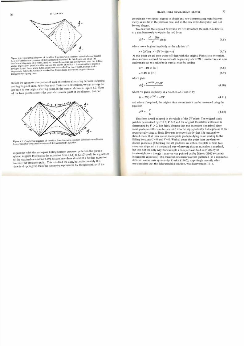
Figure 4.2. Conformal diagram of timelike 2-section with constant spherical co-ordinates
e, <{J of Finkelstein extension of Schwarzschild manifold. In this figure and in all the conformal diagrams of section 2 and section 4 the convention is employed that the Killing
vector trajectories (which in this case are the curves on which r is constant) are marked by light dotted lines, while Killing horizons are marked by heavy lines, except in that
degenerate Killing horizons are marked by double lines. Curvature singularities are
indicated by zig-zag lines .
In fact we can make a sequence of such extensions alternating between outgoing
and ingoing null lines. After four such Finkelstein extensions, we can arrange to get back to our original starting poin t, in the man ner shown in Figure 4.3. None
of the four patches covers the central crossover point in the diagram, but our
;.
Figure 4.3. Conformal diagram of timelike 2-section with constant spherical co-ordinates
e, <{J of Krushal's maximally extended Schwarzschild's solution.
experience with the analogous Killing horizon crossover points in the pseudo
sphere, suggests that just as the extension from (2.4) to (2.10) could be augmented
to the maximal extension (2.19), so also here there should be a furthe ,r extension
to cover the crossover point. This is indeed the case, but unfortunately this
time in dropping the manifest symmetry represented by the ignorability of the
BLACK HOLE EQUILIBRIUM STATES
co-ordinate t we cannot expect to obtain any new compensating manifest sym
metry as we did in the previous case, and so the new extended system will not
be very elegant.
To construct the required extension we first introduce the null co-ordinates
U, v simultaneously to obtain the null form
r2 - 2Mrds f = - du dv (4.6)
r2
where now r is given implicitly as the solution of
r+2Mlog Ir-2M1=1(u+v) (4.7)
At this point we are even worse off than with the original Finkelstein extension,
since we have restored the co-ordinate degeneracy at r = 2M. However we can now
easily make an extension both ways at once by setting
u =.,-4M In IU I (4.8)
v =4Mln IVI (4.9)
which gives
ds f = e-r/2M
dU dV
(4.10)r
where r is given implicitly as a function of U and V by
(r - 2M) er/2M = -U V (4.11 )
and where if required, the original time co-ordinate t can be recovered using the
equation
Vet/ 2 =-- (4.12)
U
This form is well behaved in the whole of the UV plane. The original static
patch is determined by U < 0, V> 0 and the original Finkelstein extension is
determined by V > O. It is fairly obvious that this extension is maximal since
most geodesics either can be extended into the asymptotically flat region or to thegeometrically singular limit. However to prove strictly that it is maximal we
should check that there are no incomplete geodesics lying on or tending to the
Killing horizo ns U =0 and V = O. We shall cover this point later on when we
discuss geodesics. [Checking that all geodesics are either complete or tend to a
curvature singularity is a standard way of proving that an extension is maximal,
but it is not the only way; for example a compact manifold must clearly be
inextensible even though it may-as was pointed ou t by Misner (l963)-contain
incomplete geodesics.] This maximal extension was first published-in a somewhat
different co-ordinate system-by Kruskal (1960), surprisingly recently when
one considers t hat the Schwarzschild solu tion, was discovered in 1916.

8/7/2019 b carter - equilibrium states of black holes
http://slidepdf.com/reader/full/b-carter-equilibrium-states-of-black-holes 12/48
---
---------
78
79B. CARTER
For studying the stationary exterior field of a collapsed star, that is to say
the classical (if it is not premature to use such a word) black hole situation, the
Finkelstein extension is sufficient, as is indicated by the conformal diagram given
in Figure 4.4. The full Kruskal extension has the feature, which seems unlikely
to be relevant except in a rather exotic situation, of possessing two distinct
asymptotically flat parts, which are connected by wha' has come to be known
as a bridge. The nature of the bridge can be under ' ,od by considering
the geometry of the three dimensional space sections, e.g. the locus U = V (which
coincides with t =0 in the original co-ordinate system) whose geometry is
suggested by Figure 4.5 which is meant to illustrate an imbedding in 3-dimensional
4".;.
6
Figure 4.4. Conformal diagram of timelike 2-section with constant spherical co-ordinates
e, .p of maximally extended space-time of a collapsing spherically symmetric star.
flat space of the 2.dimensional circumferential section 8 =7T of the locus U =V.
These three sections have spherical cross sections whose radius diminishes to a
minimum value r =2M (at the throat of the bridge) and then increases again
without bound. It can be seen from the conformal diagram of Figure 4.3 that an
observer on a timelike trajectory cannot in fact cross this throat, since aftercrossing the horizon U = 0, the co-ordinate r must inevitably continue to
decrease, until after a fmite proper time the observer hits the geometric singularity
at r = 0; this means in fact not only that such an observer is unable to reach
the region of expanding r on the other side of the throat, bu t also that he is
unable to return or even send a signal to the regions r> 2M on the side from
which he came. It is this latter phenomenon which is apparent even on the
restricted Finkelstein extension (Figure 4.2), and in the dynamically realistic
collapse diagram (Figure 4.4) which justifies the description of the nu 11 hyper
surface at r = 2M as a horizon. Thus technically, the hypersurface U = 0 is the
past event horizon of f+ , and together with the hypersurface V =0 bounding
the future of .1- , it forms the boundary of the domain of outer communications
BLACK HOLE EQUILIBRIUM STATES
which we shall denote by ~ f " } > meaning the region which can both receive signals
from, and send them back to, asymptotically large distances which in the present
case is the connected region with r > 2M specified by U< 0, V > O. The horizon
U = 0 has the infinite red shift property (which is quite generally characteristic
of a past event horizon of f+ ) that the light emitted by any physical object which
crosses it is spread out over an infmite time as seen by a stationary observer in
the asymptotically flat region, and thus not only gets infmitely red shifted as the
body approaches the horizon (which of course it can reach in a finite propertime from its own point of view) but also progressively fades out. Thus the body,
which might for example be the collapsing star represented on Figure 4.4, will
Figure 4.5. Sketch of part of a space-like equatorial 2-section (cos e =0) of one of the t =constant hypersurfaces through the throat of Kruskal's maximally extended Schwarzschildmanifold. Trajectories of the Killing vector a/a.p are indicated by light dotted lines.
appear to become not only redder bu t also blacker until with a characteristic
time of the order of that required for light to cross the Schwarzschild radius
( ~ 1 0 - 4 seconds in the case of a collapsing star of typical mass) it effectively
fades ou t of view altog ether. It is for this reason that the region inside the,horizon is referred to as a black hole.
Of course in the more exo tic situat ion when the full Kruskal ex tension is
present, the region of the past of V = 0 is by no means invisible from outside ,
and it would in fact be possible to see right back to the singularity (unless of
course, like the big bang of cosmology theory, it were hidden in some opaque
cloud of particles). The region to the past of V =0 is often referred to as a white
hole, al though with less justification than the application of the description
black to the future of U = O. Withou t worryin g about the question of colour,
it is obviously reasonable in all cases to describe the regions outside the domain
of outer communications ~ f " } > as holes.
8/7/2019 b carter - equilibrium states of black holes
http://slidepdf.com/reader/full/b-carter-equilibrium-states-of-black-holes 13/48
81B. CARTER
80
Let US now move on to see how the situation is modified in the electromagnetic
case . In the Reissner-Nordstrom solutions the timelike 2-sections have the metric
form
2 pr2 ) (r _2Mr+Q2+ 2) 2 (4 .13)ds 2 = dr2 _ dt
1 r2 _ 2Mr + Q2 + p2 r2(
When the charge is large, more precisely when Q2 + p2 >M2, this metric is well behaved over the whole range from the singularity at r =a (which from the array
(3.26) can be seen to be a genuine geometric curvature singularity) to the asymp
totic limit r 00 , and the conformal diagram is the same as in the negative M
1+
I /
I I rP"
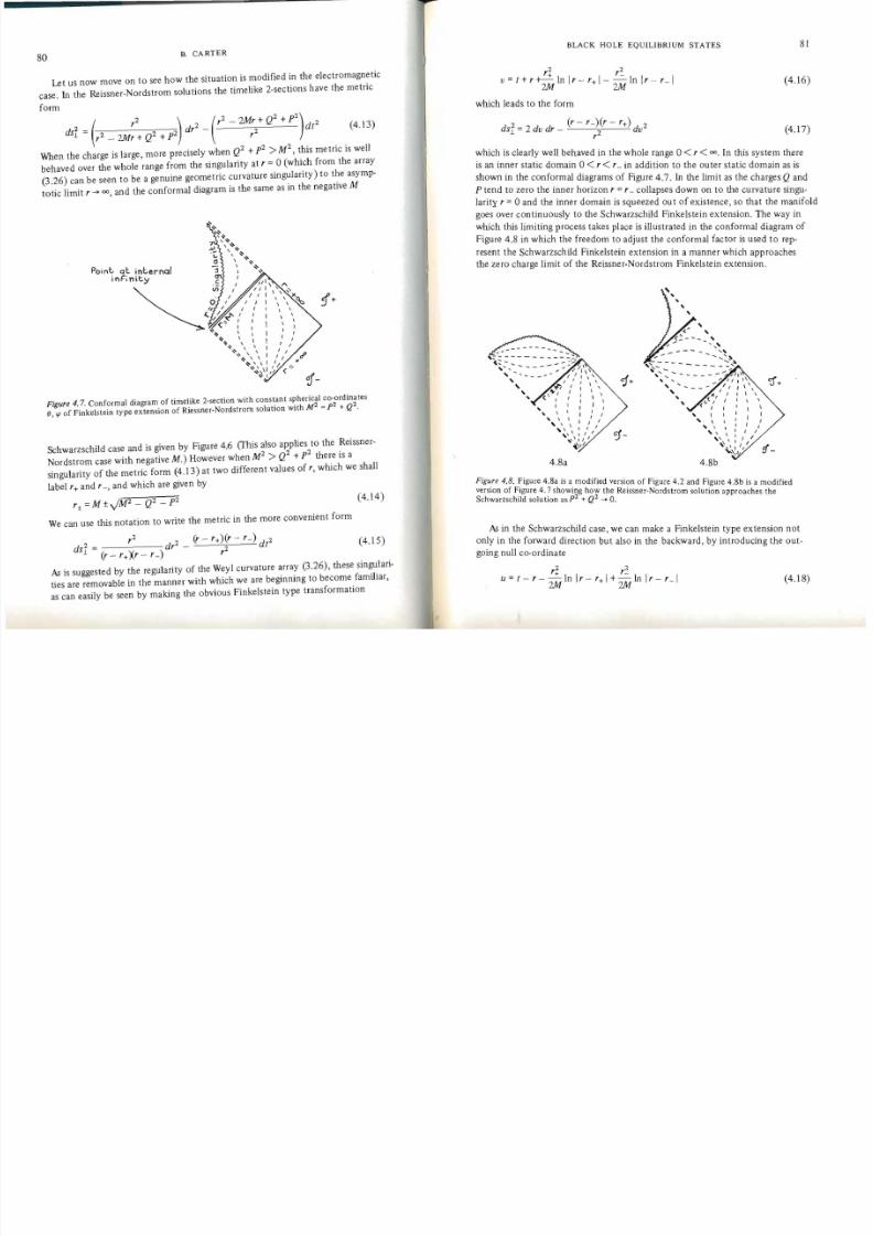
1 Figure 4.7. Conformal diagram of timelike 2-section with constant spherical co-ordinates
e, <{J of Finkelstein type extension of Riessner-Nordstrom solution with M2 =p2 + Q2.
Schwarzschild case and is given by Figure 4.6 (This also applies to the Reissner
Nordstrom case with negative M.) However when M2 > Q2 + p2 there is asingularity of the metric form (4.13) at two diff erent values of r, which we shall
label r+ and r _, and which are given by
(4.14 )r± = M ±y'M2 _ Q2 _ p2
We can use this notation to write the metric in the more convenient form
2 r2 2 (r - r+) (r - r-) 2 (4.15)dS
1= dr - - dt(r-r+Xr-r_) r
As is suggested by the regularity of the Weyl curvature array (3.26), these singulari
ties are removable in the manner with which we are beginning to become familiar,
as can easily be seen by making the obvious Finkelstein type transformation
BLACK HOLE EQUILIBRIUM STATES
r2 r2v = t + r In Ir - r+ I--=- In Ir - r_ I (4.16)
2M 2M
which leads to the form
dsr=2dvdr- (r-r_)(r-r+)2 dv
2(4.17)
r
which is clearly well behaved in the whole range 0< r < In this system there00 .
is an inner static domain 0< r < r _ in addition to the outer static domain as is
shown in the conformal diagrams of Figure 4.7. In the limit as the charges Q and
p tend to zero the inner horizon r =r _ collapses down on to the curvature singu
larity r = a and the inner domain is squeezed out of existence, so that the manifold
goes over continuously to the Schwarzschild Finkelstein extension. The way in
which this limiting process takes place is illustrated in the conformal diagram of
Figure 4.8 in which the freedom to adjust the conformal factor is used to rep
resent the Schwarzschild Finkelstein extension in a manner which approaches
the zero charge limit of the Reissner-Nordstrom Finkelstein extension.
,
, "---- ................"
..... ...........::'
"'\-- - - - - - - - ~ / \ \ \ cf '
.. ,- - - - - - - / I I \ \ 'J +1+''''', - ~ / I I \ \
' I I I \ \\
\ " " , , ( ~ I I
, < I I..
.. ,, \ \ I I
, , \ I I I , \ I
, \ \ I I I' ~ , \ : , ' I I ,, \ I I I cJ- " \ 1,;/
" \ J /~ I I I : ,',\ 1'/ d_"-'-'I;
4.8a 4.8b
Figure 4.8. Figure 4.8a is a modified version of Figure 4.2 and Figure 4.8b is a modifiedversion of Figure 4.7 showing how the Reissner-Nordstrom solution approaches theSchwarzschild solution asp2 + Q2 -+ O.
As in the Schwarzschild case, we can make a Finkelstein type extension not
only in the forward direction but also in the backward , by introducing the out
going null co-ordinate
r:u = t - r - - In Ir - r+ I+ - In Ir - r_ I (4.18)
2M 2M
8/7/2019 b carter - equilibrium states of black holes
http://slidepdf.com/reader/full/b-carter-equilibrium-states-of-black-holes 14/48
82
83B. CARTER
which leads to the form2
- 2d (r_,+)(, .- ,_)du (4.l9)dSl2 - - u d, - - ' - - - ~ -,
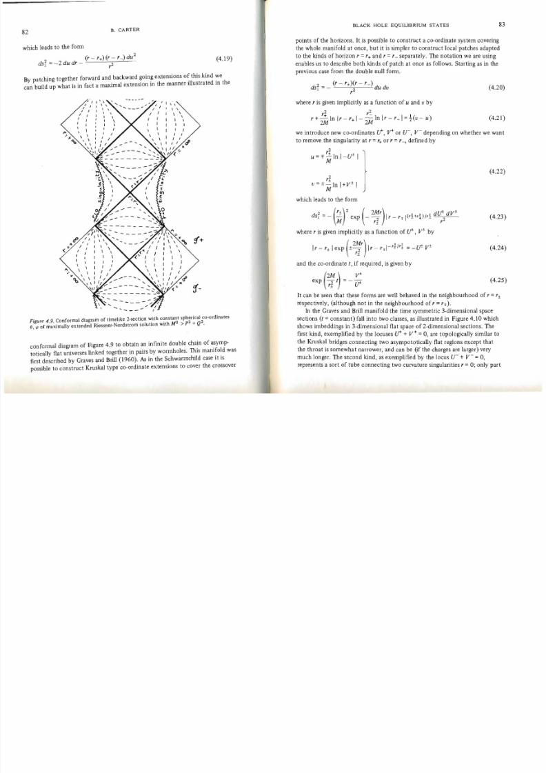
By patching together forward and backward going extensions of this kind we
can build up what is in fact a maximal extension in the manner illustrated in the
\ ,\ \\ \
\
I \I
I
<'"I
\
""
\ \
\ \
"<b
tj
.... - -
Figure 4.9. Conformal diagram of timelike 2-section with constant spherical co-ordinates
e, <{) of maximally extended Riessner-Nordstrom solution with M'l > p2 + Q2.
conformal diagram of Figure 4.9 to obtain an infmite double chain of asymp
totically flat universes linked together in pairs by wormholes. This manifold was
first described by Graves and Brill (1960). A!; in the Schwarzschild case it is
possible to construct Kruskal type co-ordinate extensions to cover the crossover
BLACK HOLE EQUILIBRIUM STATES
points of the horizons. It is possible to construct a co-ordinate system covering
the whole manifold at once, bu t it is simpler to construct local patches adapted
to the kinds of horizon, ='+ and, = , _ separately. The notation we are using
enables us to describe both kinds of patch at once as follows. Starting as in the
previous case from the double null form .
(r - , +)( , - , -) du dvdsl = - ,2 (4 .20)
where, is given implicitly as a function of u and v by
, + -'+2
In I, - , +1 - -,-2
In 1, - , - 1= 2"1 (v - u) (4.21)2M 2Mwe introduce new co-ordinates i f , r or U-, V- depending on whether we want
to remove the singularity a t , = '+ or, = , _, defined by
- , ~ +u = + - I n I- U- 1
M
(4.22)
+
v=±- In I+V-IM
which leads to the form
dif- dV±dS12= - ('±)2 exp - , ; 1,-,+ I ( r ~ + r ~ ) , r ~ M (2M') (4.23)
where, is given implicitly as a function of i f-, V± by
( 2M') " 2 +I , - ,±Iexp ± , ; I, - ,+ I - r+r±=- i f -v - (4.24)
and the co-ordinate t , if required , is given by
2M) V±(4.25)exp ( t = - if-
It can be seen that these forms are well behaved in the neighbourhood of, ='±
respectively, (although not in the neighbourhood of ' = ,+).
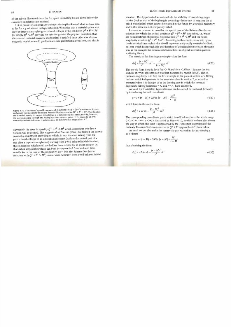
In the Graves and Brill manifold the time symmetric 3-dimensional space
sections (t = constant) fall in to two classes, as illustrated in Figure 4. JO which
shows imbeddings in 3-dimensional flat space of 2-dimensional sections. The
first kind, exemplified by the locuses if + V + = 0, are topologically similar to
the Kruskal bridges connecting two asympototically flat regions except that
the throat is somewha t narrower , and can be (if the charges are larger) very
much longer. The second kind , as exemplified by the locus U- + V- = 0,
represents a sort of tube connecting two curvature singularities, =0; only part
8/7/2019 b carter - equilibrium states of black holes
http://slidepdf.com/reader/full/b-carter-equilibrium-states-of-black-holes 15/48
8485B. CARTER
of the tube is illustrated since the flat space imbedding breaks down before the
curvature singularities are reached.Let us pause for a moment to consider the implications of what we have seen
so far for a gravitational collapse situation. We notice that a material sphere can
only undergo catastrophic gravitational collapse if the condition Q2 + p2 <M2
(or simply Q2 <M2 provided we take for granted the physical condition that
there are no material magnetic monopoles) is satisfied since otherwise electro
magnetic repulsion w0uld predominate over gravitational attraction, and that it
r : r ~
------- .....
Figure 4.10. Sketches of spacelike equatorial 2-sections (cos 8 =0) of t =constant hypersurfaces in the maximally extended Reissner-Nordstrom when M2 > pZ + QZ. The sketchesare rntended loosely to suggest imbeddings in 3-dirnensional flat space ; strictly, however,
the section passing through the Killing horizon crossover point r = r - ceases to be symmetrically imbeddable when it gets too near to the curvature singularity r = O.
is precisely the same in equality Q2 + p2 <M2 which de termines whe ther a
horizo n will be formed. This suggests wha t Penrose (1969) has termed the cosmic
censorship hypothesi s according to which, in any situation arising from the
gravitational collapse of an astrophysical object (such as the central part of a
star aft er a supe rnova explo sion) startin g from a well behaved initial situatioT1,
the singularities which result are hidden from outside by an event horizon Le.
that naked singularities which can both be approached from and seen from
outside (as in the case of the singularity at r =0 in the Reissner-Nordstrom
solutions with Q2 + p2 >M2) cannot arise naturally from a well behaved initial
BLACK HOLE EQUILIBRIUM STATES
situation. This hypothesis does not exclude the visibility of preexisting singu
larities (such as that of the big bang in cosmology theory not to men tion the so
called white holes) which cannot be reached in the fu ture by a timelike trajectory
and in this sense are not completely naked.
Let us now move on to consider the special case of the Reissner-Nordstrom
solutions for which the critical condition Q2 +p2 = is satisfied, Le_ which
are poised between the normal hole situation Q2 + p2 <M2 and the naked
singularity situation Q2 + p2
>M2. According to the cosmic censorship hypo
thesis a critical case such as this should represent a physically unattainable limit,
but one which is approachable and therefore of considerable interest in the same
way as for example the extreme relativistic limit is of great interest in particle
scattering theory .
The metric in this limiting case simply takes the form
(r M)2ds2
= - dr2 -.1 r2
r2- - -= - d t2(r _ M)2
(426).
This metric form is static both for r >M and for r <M but it is none the less
singular at r =m. Its extension was first discussed by myself (1966). The co
ordinate singularity is in fact the first example in the present section of a Killing
horizon which is degenerate in the sense described in section 2, as would be
expected when it is thOUght of as the limiting case in which the two non
degenerate Killing horizons r =r+ and r =r_ have coalesced.
As usual the Rnkelste in type extens ion can be carried ou t wi thou t difficulty
by introducing the null co-ordinate
M2v= t+ ( r -M)+2Mln l r -MI - - - (4.27)
r -M
which leads to the metric form
dsl = 2 dr dv _ (r -2M)2 dv
2 (4_28)r
The corresponding co-ordinate patch which is well behaved over the whole range
0< r<
0 0, _00
<v
<00 , is illustrated in Figure 4.10, in which we have also shown
the way in which this limit is approached by the Finkelstein extensions of the
ordinary Riessner-Nordstrom metrics as Q2 + p2 approaches M2 from below.
As usual we can also make the symmetric past extension, by introducing a
co-ordinate
M2u= t - ( r -M ) - 2M l n l r -M I+ - (4.29)
r -M
thus obtaining the form
d2 2 d (r - M)2 d 2
s.1 = - u dr - --- r (4.30)r2

8/7/2019 b carter - equilibrium states of black holes
http://slidepdf.com/reader/full/b-carter-equilibrium-states-of-black-holes 16/48
8786 B. CARTER
This time however there is no way of carrying out a further Kruskal type exten
sion, because the transformation (4.27) contains not only the by now familiar
logarithmic singularity but also a first order pole singularity. However it turns
out that a Kruskal type extension is quite unnecessary, since the Finkelstein
extensions can be fitted together in the manner illustrated in Figure 4.1.2 to form
an extended manifold which is in fact maximal since (as we shall verify later) all
geodesics either in tersect the curvature singularity or can be completed. The
situation is rather different from those which we have come across so far, because
,
7' \ ".» \ ,.' \ ,
\.. \ ,.J' \ ,
:l
"
- - ~ : ~ = ~ - ; : I <, '.........- - , "- --;"-,/1\",, "
,",,'" / I I \ \
1+, I \ \,, I \ \
\, \
,, I
'\ I I
'\ I I '
,,'I / ':1' \ \ I I
",1/1
" I /
Figure 4.11. Conformal diagram of timelike 2-section with constant spherical co-ordinatese, <p of Finkelstein-type extension of Reissner-Nordstrom solution in degenerate case whenM'l =p2 + Q2.
the completed geodesics can not only approach the outer parts of the diagramlabelled and Y-, but can also approach the inner boundary points labelled x,
each of whlch therefore represents (in a manner which is disguised by the
conformal factor) infinitely distant limit in the inward direction.
The nature of the limits represented by the points x, (whlch take the place
of the missing Kruskal crossover axes) can best be understood by co nside ring the
time symmetric space sections, t = constant. In this case the analogue of Figure
4.10 is given by Figure 4.13 which shows that instead of having a minimum (the
throat) or a maximum of r in the respective cases r >M, r <M, the space sections
extend indefinitely, both approaching asymptotically the same infmite spherical
cylinder.
BLA CK HOLE EQUILIBRIUM STATES
\
\
I
1
\ ..
\ \ , , ~ 1+
I
I
#I ''/
I
( f\ \ ' I X
\ t I, "
.11 1/ ( B-Figure 4.12. Conformal diagram of timelike 2-section with constant spherical co-ordinates e, <p of maximal extension of Reissner-Nordstrom solution in degenerate case when M'l =p2 + Q2 .
f fA'"'I\..
"- -
'U ~ ~ - - - J r--fJ, \
....
3
Figure 4.13. Sketches of spacelike equatorial 2-sections (cos e =0) of r =constant hypersurfaces in the maximally extended Reissner-Nordstrom solution in the case M'l =p2 + Q2
and also in a RObertson-Bertotti universe, indicating how the latter represents an asymptotic limit of the former.

8/7/2019 b carter - equilibrium states of black holes
http://slidepdf.com/reader/full/b-carter-equilibrium-states-of-black-holes 17/48
8988 B. CARTER
It is at this stage that the Robinson-Bertotti solution (3.34) enters into the
discussion. We do not need to do any further work to find its global structure,
since its time sections have the metric
dSI = (Q2 +p2) _A? dT2) (4.31 )
which, as we have already remarked is the metric of a pseudo-sphere, so that the
1
1 4 ~ 4.l4b
Figure 4.14. Figure 4.14a represents a modified version of Figure 4.12 and Figure 4.14b
represents a modified version of Figure 2.2b. The shaded regions of the two diagrams canbe made to approximate each other arbitrarily closely in the neighbourhood of the horizons,
showing that the maximally extended Reissner-Nordstrom solution effectively contains a
Robertson-Bertotti universe within it in the bottomless hole case when M'2 = p2 + Q2.
required extension past the singularity 11.= 0 is given by (2.19) and the corre
sponding conformal diagram is that of Figure 2.2b. Now it can easily be seen by
setting r = 11.+ M, t = M2T, that the Reissner-Nordstrom solution with Q2 +.p2 =M2
approaches the Robertson-Bertotti solution in the asymptotic limit as r .... 00 .
The limiting spherical cylinder illustrated in Figure 4.13 is in fact the same as a
T = constant cross section of a Robinson-Bertotti universe. The conformal diagrams
of the Q2 + p2 =W Reissner-Nordstrom solution, and of the Robinson- Bertotti
solution are shown side by side for comparison in Figure 4.14. The shaded regions
BLACK HOLE EQUILIBRIUM STATES
A g"+".0
\
\\
\I
I
1
Figure 4. 6. Conformal diagram of timelike 2-section with constant spherical co-ordinates
0 , 'P in the maximally extended Reissner-Nordstrom solution in the naked singularity case when M'2 < p2 + Q2.
can be made to coincide as closely as one pleases by adjusting the conformal
factor so that they correspond to a sufficiently small range of the co-ordinateA=r-M.
5 Derivation of the Kerr Solution and its Generalizations
Having now looked fairly thoroughly at the spherical vacuum solutions, we have
clearly arrived at a stage where it would be interesting to see how the various
phenomena-horizons, naked singularities etc.-which we have come across would
be modified in more general non-spherical situations, particularly when angular
momentum , the most obvious source of deviation from spherical symmetry, is
presen t.
Since, as we have seen, the derivation of the spherical Schwarzschild solution
is very easy (it was achieved in 1916 wit hin a year of the publication of Einstein's
Theory in 1915) one might have guessed that it would be comparatively not too
difficult to derive a rotating (and hence non-static but still stationary) generaliza
tion in a fairly straightforward manner , starting from some suitably simple and
natural canonical metric form. Moreover, as I plan to make clear in this section,
one would have guessed correctly. l'°evertheless, after forty years, repeated
attempts to find a canonical form leading to a natural vacuum generalization of
the Schwarzschild solution had turned up nothing (or more precisely nothing
which was asymptotically flat) except the Weyl solutions, which are unfortunately
static, and therefore useless in so far as showing the effect of angular momentum
is concerned. Moreover the first (and so far the only) non-static pure vacuum
generalization of the Schwarzschild solu tion was found at last by Kerr in 1963

8/7/2019 b carter - equilibrium states of black holes
http://slidepdf.com/reader/full/b-carter-equilibrium-states-of-black-holes 18/48
9190 B. CARTER
using a method which is by no means straightforward, and which arose as a bi
product of the sophisticated Petrov-Pirani approach to gravitational radiation
theory which was developed during the nineteen fifties. In consequence of this
history it is still widely believed that the Kerr solution can only be derived using
advanced modern techniques. There is however an elementary approach of the
old fashioned kind which was rather surprisingly overlooked by the searchers in
the nineteen twenties and thirties, and which I actually found myself, with the
aid of hindsight, in 1967. This approach now seems so obvious that la m sure it
will be clear to anyone who follows it that despite the apparent messiness of the
form in which it is customarily presented, no non-static generalization of the
&hwarzschild solu tion which may be discovered in the fu ture can possibly be
simpler in its algebraic structure than that of Kerr.
This approach starts from the observation that for practical computational
purposes one of the most useful, indeed almost certainly the most useful, algebraic
property which the Schwarzschild solution possesses as a consequence of
spherical symmetry, and which one might hope to return in a simple non-spherical
generalization, is that of separability of its Dalembertian wave equation and the
associated integrability of its geodesic equations.
Now it is physically evident from the correspondence principle of quantum
mechanics, (and it follows mathematically from standard Hamilton Jacobi
theory) that integrability of the geodesics as well, obviously, as separability of
the Dalembertian wave equation I/;;a;a =0, will follow if the slightly more general
Klein-Gordon wave equ ation I/;;a;a - m21/; =°(where m2 is a freely chosen
constant which may be interpreted as a squared test particle mass) is separable.
Separability is of course something which depends not only on the geometry
bu t on a particular choice of co-ordinates x 2 (a =0, 1, 2, 3), and in terms of these
co-ordinates it depends less directly on the form of the ordinary covariant tensor
gab defined by
ds2 =ga b dx
adx b
(5.1 )
than on the form of the contravariant metric tensor defined in terms of the
inverse co-form
a)2 _ a a(5.2)(as - axa axb
In terms of the contravariant metric components and of the determinant
g= det (gab)= {det«b)f l (5.3)
the Klein Gordon equation can be expressed in terms of simple partial derivatives
in the form
V I ~ y C i ~ b 1/;- m 2 y1-i=0 (5.4)bax .
BLACK HOLE EQUILIBRIUM STATES
The standard kind of separability takes place if substitution of the product
expression
I/; = I / ; i (5.5)
where each function I/; i(i = 0, 1, 2, 3) is a function of just the single variable xi,
causes the left hand side of (5.4) to split up into four independent single variable
ordinary differential equations, expressed in terms of four independent freelychosen constants of which 1112 is one.
To see how this works out in the spherical case, we note that the inverse metric
corresponding to our general spherical canonical form (3 .2) is
(a)2 1 { 2 (a)2 1 ( a )2 (a)2 Z;( a )2} (5.6)as = r2 (l - J.1 ) aJ.1 + 1 - J.12 a", + /:"r ar - /:"r at
and hence using (3.3), the Klein Gordon equation takes the form
C
{VI(l_J.12)al/; +
Vi_ 1 _ ~ 1 / ; _ m2r2}
Zr aJ.1 aJ.1 1 - J.12 a",2
+1/;-1 ~ r 2 / : " r a l / ; _1/;-1 rZra21/;=0(5.7)
ar Zr ar /:"r at2
which has solutions of the form
iw tI/; = R r P ~ ( J . 1 ) e i n < P e (5.&)
where t, n, ware separation constants (o f which t and n must be integers if the
solution is to be regular) and (J.1) is a solution of the (t, n) associated Legendre
equation (and is thus an associated Legendre-polynomial in the regular case) and
where Rris
a solu tion of the equation
2 2Z 2 2-I d r 2 / : " r d R r + ~ + ~ [ t ( l + 1 ) _ m 2 r ]=0 (5.9)Rr dr Zr dr /:"r Zr
What we want to do now is find the simplest possible non-static generalization
of the canonical coform (5.6), including in our criteria for simplicity no t only the
most obviuus requirement of all, namely that the manifest symmetry property of
stationarity and axisymmetry represented by the ignorability of the co-ordinates
t and", be retained but also the requirement that the separability property of the
corresponding Klein Gordon equation be retained. There is a third obvious
8/7/2019 b carter - equilibrium states of black holes
http://slidepdf.com/reader/full/b-carter-equilibrium-states-of-black-holes 19/48
9392 B. CARTER
simplicity property of the coform (5.6) which can be retained without prejudice
to the other two, (and which greatly simplifies the computation of the Riemann
tensor etc.) namely the fact that it determines a natural canonical orthonormal
tetrad, such that two of the tetrad vectors contribute in the separation only to
the terms independent of r, while the other two contribute only to the terms
independent of /1.
This leads us to try the canonical coform
a) 2 1 { ( a )2 I [a a ] 2}( as = Z !:lJ.l. a/1 + !:lJ.l. ZJ.I. at + QJ.I. a",
1 { (a )2 1 [a a ]2} (5.10)+Z !:ly ar - !:ly Zy at + Qy a",
where !:lJ.l., ZJ.I., QJ.I. are functions of /1 only, and where !:ly, Zy, Qy are functions of
r only, and the form of the conformal factor Z remains to be determined.
It is to be observed that the factors !:lJ.l. are redundant, since the one in the
first term could be eliminated by renormalizing /1 as a function of itself while the
one in the second term could be eliminated by a proportional readjustment of
ZJ.I. and !:lJ.l.. The same applies to the factor !:ly. These factors have been included
explicitly however firstly because they are suggested by the canonical spherical
coform (5.6) (to which (5.10) reduces when one sets !:lJ.l. = 1 - /12 with /1 = 1,QJ.I. =Qy =0 and Z =r2) bu t also for the more compelling reason that the
freedom of adjustment of !:lJ.l. and !:ly can be used to achieve considerable simplifica
tion of the form of Z required to achieve separability. In any case they are
arranged so as to cancel out of the determinant which is simply given by
Z2(5.11 )
vC i = IZyQJ.I. - ZJ.l.Qy I
Let us now investigate the conditions which must be imposed on Z to achieve
separability. Using (5.10) and (5.11) we obtain the Klein Gordon equation in the
form
VI { ~ - £ i . ! : l vCi!: l vC i m2Z}t/Ia/1 Z J.I. a/1 ar Z y ar Z
I a (- Ci) (a+V [ -Q +-za} -1 Q -+ z -a ) t/Ia", J.I. at J.I.!:lJ.l. Z J.I. a", J.I. at
- t/I - I ( - Q + a )Z -I - Q - +Z -a ) .r, =a - (Fi) (a 0 (5.12)a", y at Y!:ly Z y a", y at 'I'
It is clear that if these terms are to separate, the factor Z-IFi which occurs in
each one must depend on r and /1 only as a product of single variable functions
which can be absorbed into !:ly and !:lJ.l. (using our freedom to rescale these
BLACK HOLE EQUILIBRIUM STATES
functions) so as to reduce the factor Z-IFi to unity. Thus we are led to
choose the definition
Z=ZyQJ.I.-ZJ.l.Qy (5.13)
for the conformal factor. This is still not quite sufficient for separability except
in the case of the pure Dalembertian wave equation, since there remains the mass
term which now takes the form m2Z. In this expression we have not only made no
provision for cross terms between the non-ignorable co-ordinates, i.e. termsproportional to (a/ar)(a/a/1), which would obviously destroy the separability,
but we have also, in accordance with our principle of maximum simplicity, ex
cluded all other cross terms except those directly between the ignorable co
ordinates, i.e. those proportional to (a/at)(a/a",) whose presence is essential if
we are to have non-zero angular momentum. To achieve complete separability
this term also must split up into the sum of two parts each depending on only
one variable, i.e. Z must have the algebraic form
Z = UJ.I. + VA (5.14)
where UJ.I. depends only on /1 and VA only on A. From the expression (5.13) we
see that this requirement will be satisfied if and only if
dZ ydQJ.I. dZJ.I. dQy_------0 (5.15)dr d/1 d/1 dr
There are basically two ways in which this can be satisfied: a more general
case in which either both Zy and ZJ.I. or both Qy and QJ.I. are constants, and a
more special case in which at least one of the four functions is zero, or can
be reduced to zero by a form preserving co-ordinate transformation in which <p
and t are replaced by linear combinations of themselves. In the more general
case we can take it without loss of algebraic generality that it is the Q's which
are constants. Thus replacing Qy, QJ.I. by constant Cy, CJ.I. respectively we obtain
the basic separable canonical form
- - 1 {( a )2+-
1 C-+Z -
a ] 2}a )2 !:l [a( as - [CJ.l.ZY - cYZJ.l.l J.I. a/1 !:lJ.l. J.I. a", J.I. at
+ 1 (a- - -I [aC -+z !:l a ]2} (5.16)[CJ.l.zy - cyzJ.l.l y ar !:ly y a", y at
The original expression (5.10) from which we started had algebraic symmetry
not only between rand /1 (apart from a sign change) bu t also between t and "'.
In the coform (5.16), in which the symmetry between t and '" has been lost, we
have chosen to set Qy and QJ.I. rather than Zy and ZJ.I. constant in order that it
should include the spherical coform (5.6), in which t and '" have their usual

8/7/2019 b carter - equilibrium states of black holes
http://slidepdf.com/reader/full/b-carter-equilibrium-states-of-black-holes 20/48

8/7/2019 b carter - equilibrium states of black holes
http://slidepdf.com/reader/full/b-carter-equilibrium-states-of-black-holes 21/48
97B. CARTER96
it is clear that we need h> 0 and also hp + q2 > O. Now we know that if the
symmetry axis is to be well behaved the overall coefficient of d,/ in the metric
form (5.18) must be zero that is to say ZjJ must vanish for the same values of f.l
as f:l. jJ . Now the values of ZjJ and Zr may be adjusted to the extent of the
addition of the same arbitrary constant to both of them (by replacing t by a con
stant coefficient linear combination of t and..p) but it is clear that even with
these adju stmen ts the zeros of Z jJ will always occur for equ al and opposi te
values of f.l, and can therefore match the zeros of f:l.jJ only if q is zero. Thus wesee that the restri ctions
(5.28)q=O
(5.29)h>O
(5.30)p
are necessary for regular angular behaviour of the solutions. When the two latter
conditions are satisfied we can make scale changes of f.l and r so as to obtain
h = p 1 thereby ensuring that f.l varies over the conventional co-ordinate
range -I < f.l < I . In doing so we use up our co-ordinate freedom to adjust a
which thereafter becomes a geome trically well de termined parame ter). The
adjustment of t and..p necessary to ensure that the zeros of ZjJ coincide with
those of f:l.jJ leads us to replace the forms (5.25) of the solu tion (which were
previously adjusted for maximum algebraic simplicity) by
Zr =r2 + a2 (5.31)
ZjJ =a(1 - f.l2) (5.32)
while the other conditions we have imposed cause the expressions (5 .26) , (5.27)
to reduce to the standard expressions
2 ( 5.33)t::.r =r2 - 2M r + a
t::.jJ = 1 - f.l2 (5 .34)
On substituting these expressions together with (5.23) and (5.24) back into the
canonical form (5.18) and making the su bstitu tion
(5 .35)f.l = cos fJ
we obtain the solution of Kerr (1963) in the standard co-ordinate system intro
duced by Boyer and Lindquist (1966), which takes the explicit form
22
ds2 =(r2 + a2 cos2fJ) { dr + dfJ }2r2 _ 2M r + a
sin 2fJ (a dt - (r2 + a2) d..p]2 - (r2 - 2M r +a2) [dt - a(1 - f.l2) d..p]2
+ - - - - ~ - - - - ~ ~ ~ ~ - - ~ - - - - ~ - - ~ - - ~ ~ ~ r2 + a2 cos2
fJ
(5.36)
BLACK HOLE EQUILIBRIUM STATES
where we have retained the grouping of the terms to make manifest the canonical
tetrad with respect to which the separability (which of course is no t affected by
the replacement of f.l by a function of itself) takes place. In terms of this tetrad
as given explicitly by (5.19), (5.20), (5.21), (5.22) and of the curvature forms
defined in section (3), the Weyl tensor, which in this case is equal to the Riemann
tensor , may be presented in the form
Q(1)(2) =-I
I w(l ) A w(2) - 12 w(O) A w(3)
Q(O)(3) = - I l dO) Aw(3) + I2dl ) AW(2 )
Q(O)(I ) =2I I dI ) A dO ) - 2I2 d 2) A d 3)
Q(3) (2) = 21 I W(2) A w(3) + 212 w(l ) A w(O) (5.37)
Q(O)(2) = I I d 2) A dO ) - 12d l ) A w(3)
Q(3)( l ) = II w(I) Aw(3) + I d 2) A w(O)2
where
2 2)(r2 - 3a f.l ,(5.38)
II =M r (r2 +a2f.l2)
(3 r2 -a 2f.l2)(5.39)
12 =Maf.l (r2 + a2f.l2)3
It is obvious (to an expert) from this array that the canonical separation tetrad
is also a canonical Petrov tetrad, and that the Weyl tensor is of Petrov type D. It
was by searching for vacuum solutions with type D Weyl tensors that Kerr originally
found this metric .
Let us now move on to consider the electromagnetic generalization of the
method we have just applied. The obvious thing to do is to seek a generalization
of the spherical canonical form (3.32) to canonical form of the electromagnetic
potential A in a separable background metric of the canonical form (5 .18) which
will be such that not only the ordinary Klein Gordon equation but also its
electromagnetic generalization is separable, thus ensuring (as a consequence of
Hamilton-Jacobi theory, or from a physical point of view by the correspondence
principle) that not only geodesics but also charged particle orbit s will be
integrable. In terms of an electromagnetic field potential
A=Aa dxa (5.40)
the electromagnetic Klein-Gordon equation takes the form
r l ( a ~ -ieAa) v=ggLIb (a!a - ieAa) W- m2 W= 0 (5.41)
8/7/2019 b carter - equilibrium states of black holes
http://slidepdf.com/reader/full/b-carter-equilibrium-states-of-black-holes 22/48
9998 B. CARTER
In order not to introduce unnecessary cross terms we shall start off by requiring
that A contain only the same two components as were necessary in the spherical
case, i.e. that it has the form
A =A 3 d<.p +A 0 dt ( S.42)
where A 3 and Ao are scalars, independent of <.p and t, whose functional dependence
on IJ. and r remains to be determined. On substituting this expression into (3.41),
using the canonical co·form (S.18) we obtain
- I {a a a a 2 }tJ; -6 . J1 . -+-6 . , - - m (CJ1.Z,-C,ZJ1.) tJ;aIJ. aIJ. ar ar
_ {a a .} 1 {a a }+ tJ; I -a Z J1. + -a CJ1. + leX J1. -;;;- - Z J1. + - CJ1. + ieX J1. tJ;t <.p UJ1. at a<.p
a } a }'I' {at' a<.p' , 6., at a<.p
_, / , -1 -Z + -Ca - ieX - l { a-Z ,+ -C , - l eX ,. tJ;=0 (S.43)
where we have set
AoZ,+A3C,=X, }(S.44)
A oZJ1. +A 3C
J1. = -XJ1.
In order for the equation to separate we clearly need to choose A 0 and A 3 in
such a way that X J1. and X, are respectively functions of IJ. and r only. This can
be done simply by taking arbitrary functions X" X J1. of rand IJ. respectively and
solving (S.44) for A 0 and A 3' Thus we obtain the expression
A =X,(CJ1. dt - ZJ1. d<.p) + XJ1.(C, dt - Z, d<.p)(S.4S)
CJ1.Z, - C,ZJ1.
for the canonical separable vector potential associated with the form (S.18). We
can now go on to solve the source free Einstein-Maxwell equations for the forms
(S .4S) and (S.18) in conjunction, using the method described in section 3. As in
the pure vacuum case the functions 6.J1., 6." Z" ZJ1. turn ou t to just quadratic
polynomials, and the new functions X" XJ1. are even simpler- they are linear.Again there is a large class of solutions most of which have undesirable global
behaviour, and from which a small subclass can be selected by requiring thatIJ.
should be a well behaved azimuthal angle co-ordinate. We shall not repeat this
selection procedure but merely present the final form of the well behaved sub
class, using the same normalization conditions as in our presentation of the
vacuum Kerr solutions. Thus the solutions for which C, or CJ1. are non-zero are
given directly, setting
CJ1. = 1 (S.46)
C, =a (S.47)
BLACK HOLE EQUILIBRIUM STATES
by
X, =Qr (S.48)
XJ1.=PIJ. (S.49)
2Z, =r2 +a (S.SO)
ZJ1. = a( l - IJ.2) (S.SI)
6., =r2 _ 2Mr + a2 + Q2 + p2 (S.S2)
6.J1.=1-IJ.2 (S .S3)
where in addition to the parameters M and a which by comparison with the Lenz
Thirring solu tion can be seen to represen t mass and angular momen tum per uni t
respectively, we now have two more parameters Q and P which represen t electric
and magnetic monopole moments. This solution was first obtained by Newman
and his co-workers (196S) using a guessing method based on an algebraic trick.
Written out explicitly, and again setting IJ. = cos e, this Kerr-Newman solution
takes the standard form
ds2 =(r2 + a2 cos2e) ( dr2
+de2}r2 _ 2Mr + a2 + Q2 + p2
sin2e[a dt - (r2 + a2) d<.p]2 - (r2 - 2Mr + a2 + Q2 + p2)[dt _ a sin2e d<.p)2
+ - - - - - - ~ - - - - ~ ~ - - ~ - - ~ - - ~ - - ~ - - ~ ~ - - - - - - - - ~2r2 +a2 cos e
( S.S4)
with
A = Qr[dt - a sin2e d<.p) +P cos e [a dt - (r2 + a2)d<.p]
(S.5 S)r2 +a2 cos2e
[These soluti ons can be obtained from the general soluti on [A] (Carter 1968) by
making the restrictions q =0, h > 0, p > 0 and setting r =A, a cos e =IJ., <.p =atJ; ,2
t =X+ a2
tJ; where a = p.] The metric (but not of course the field) is invariant
under a duality ro ta tion in which a and b are altered in such a way as to preserve
the value of the sum of their squares. The Ricci tensor for this metric can be ,
expressed in terms of the canonicaI'tetrad as
Q2 +p2 R b = [w(O)w(O) + w(3 )wO) + w(2)w(2) - w(l )w( l»)
a r2 + a2IJ.2 a b a b a b a b (S.S6)
and the Weyl tensor has the same basic form (S.37) as in the vacuum case, but
this time with the more general expressions
Mr[r2 -3 a2IJ.2)_(Q2 +p2)(r2 _ a2IJ.2)II = - ~ - - - - ~ - 7 - - ~ ~ ~ ~ - - - - ~ ~ (S .S7)
(,-2 +a2J..l2)3

8/7/2019 b carter - equilibrium states of black holes
http://slidepdf.com/reader/full/b-carter-equilibrium-states-of-black-holes 23/48
100
101
B. CARTER
Mall [3r2 - a21l2] - 2(Q2 +p2)1!J.f (5.58)
1 2 = - - ~ - - - - - - ~ - - ~ ~ - - ~ ~ (r2 + a211
2)3
for the coefficients.We now come to the special case-the generalization of the Robinson-Bertotti
solution-which has been left ou t so far. These special cases can be obtained
from the general form by making the linear co-ordinate transformation r 4 cr + k
and then taking the singular limit when c tends to zero . Again we select a subsetfrom a much wider class by the requirement that 11 should behave as a regular azi
muthal co-ordinate. The solutions could be expressed algebraically in terms of
the general canonical form (5.18) bu t it would be geometrically misleading to do
so since t and <p would come the wrong way round . Instead we express the
solution directly in an alternative and in this case geometrically more enlightening
canonical form as follows. [These solutions can be obtained from the form [B( -) ]
(Carter 1968) in the subcase q = 0, h> 0, k2> Q2 + p2 by adjusting m to zero,
n to unity, setting a2 =k2 - Q2 - p2 and replacing 11 by all, I/J by t and ax by
(a 2 + k2)<p]
dA2
dll2 2}ds2 = (a21l2 + k2) - + - - I:::..A dr
( I:::.. A 1:::../1
I:::.. (5.59)+ /1 [( 2 2a21l2+k2 a +k )d<p- 2ak'Adr]2
with
2 2A = Q'Adr +p [(a + k ) d<p - 2ak'A dr] (5.60)
/1 a21l2+e
where
I:::.. =1 - 112 \ (5.61)
1:::..: = 'A2+ n f
where Q, P, a, n are independent parameters, of which the last, n, canbe adjusted to zero by suitable bu t non-trivial form preserving co-ordinate tranS
formations using the fact that the solution has a 4-parameter isometry group (o f
which only 2 degrees of freedom-those corresponding to the ignorability of t
and <p- manifest) under which the hypersurfaces on which 11 is constant areare
homogeneous and partially isotropic. The parameter k is not independent of the
others, bu t must satisfy(5.62)
k2 = a2 + Q2 + p2
[These solutions are no t fundamentally new since they could have been obtained
from Taub-N.U.T. space (in the case where the "mass" term is zero) by analytic
BLACK HOLE EQUILIBRIUM STATES
continuation in complex co-ordinate planes-the parameter k turning up as the
analogue of the standard N.U.T. parameter I.]In a more explicit form , having chosen n = 0, and having set 11 = 0, these
solutions can be expressed as
ds 2= [a
2(l + cos28) + Q2 + p2] + d82 _ 'A2 dr2}
sin28 [(2a 2 + Q2 + p2) d<p _ 2a(a2 + Q2 + p2)1/2 'A dr]2+ (563)
[a2(l + cos28) + Q2 + p2] .
with
2A =Q'A dr +P cos 8 [(20
2+ Q2 + p2) d<p - 2a(a + Q2 + p2)1/2 'A dr]
[a2(l + cos28) + Q2 + p2]
(5.64)
which clearly reduces to the Robinson-Bertotti metric when a is set equal to
zero.
The derivation of the source-free solutions of the separable form (5.18) with
(5.45) worked out so well , and the separability property is so valuable for sub
sequent applications, that I was tempted to go en and search for more general
solutions, in which for example, a perfect fluid is present. Unfortunately the
separability conditions are in fact very restrictive-so much so that it is rather
remarkable that there are any vacuum solutions at all-and nothing that was of
any obvious physical interest turned up (not that I would by any means claim to
have exhausted the subject). However, there was one generalization which came
out at once, namely to solutions with no material sources but in which a cosmo
logical A term is present. Although I don't think there is much physical justifica
tion for believing a non-zero A term, it is perhaps worth quoting the result as a
geometrical curiosity. When a A term is present the solutions are still polynomials,
Xr and X/1 being linear and Zr and Z/1 being quadratic, as before, but now I:::.. r and
1:::../1 are no longer quadratic but quartic. As before, the solutions which I quote
below are selected ou t of a much wider class by the requi remen t that 11 should
behave as a regular and azimuthal angle co-ordinate, which ensures that the
solutions tend asymptotically this time not to Minkowski space as before butto de-Sitter space. The pure vacuum solutions are given by
2 22 2 dr d8 }
ds = (r2 + a cos 8) - + 1 2 A 28{ I:::.. r 1 - "3a cos
2. (I - ~ a 2 ACOS2 8) [a dt - (r2 + a ) d<P]2
+ SJD 28r2 + a2 cos28 I - ~ a 2 A
I:::..r [dt-asin28d<P]2(5.65)
r2 + a2 cos2e 1 - A

8/7/2019 b carter - equilibrium states of black holes
http://slidepdf.com/reader/full/b-carter-equilibrium-states-of-black-holes 24/48
102 B. CARTER
where
boy =jA(r4 +a2r2) + r2 - 2Mr + a2 (5.66)
A straightforward electromagne tic generalization exists, bu t I shall no t bother to
write it ou t here. [This solution can be obtained from the general solution [A]2
(Carter 1968) by setting q =0, p =a , h = 1 + A wi th the restriction
1 - A> 0, and setting r =A, a cos e =jJ., <p =a( 1 - ~ a 2 A)1j; and
t = (1 - A)(X + a21j;)] .
This solution has the property that it can be expressed in the form
222M [ dt - a sin2e d(p dr] 2
ds = ds 0 + r - ----=----=-------,---=(1 -1a2 A)(r2 + a2 cos2e) (r2 + a2)(1 + ~ A r 2 )
(5.67)
where
22 dr2 de }2
d s ~ = (r2 + a cos e) {(a2 + r2)(1 + ~ A r 2 ) + I _ A cos2e
2. 2 (1 - A cos
2 el [a dt - (r2 + a ) d<P]2 (5.68)+ Sin e r2 + a2 cos2e) (1 -1Aa 2
)
where the new time and angle co-ordinates 7and (p are defined by
2Mrdr(5 .69)
dt = dt + (1 + 1Ar2) boy
a) 2Mr dr (5.70)dIP = d<p + ( r2 + a2 (1 + 1Ar2) boy
The form whose square appears in the second term of (5.67) is in fact a null form ,
either with respect to the ful1 metric ds 2or with respect to the metric d s ~ to
which ds 2 reduces when m is set equal to zero. The existence of the expression
(5.67) establishes the claim that the solution is asymptotical1y de·Sitter (or
2asymptotically flat when A =0) since the metric d s ~ to which ds tends in the
limit is in fact exactly de-Sitter space (o r exactly Minkowski space when A = 0)
albeit in a somewhat twisted co-ordinate system. The co-ordinate system may be
un twisted, and (5.68) reduced to a familiar expression for de-Sitter space (or
flat space when A = 0) by in troducing new co-ordinates F, e, .p, i defmed by
(1 -1a2 A)f2 =r2 + a2 sin2e -1a2 Ar 2 cos2e (5.71)
f cos {j = r cos e (5 .72)
___ + ~ a A t (5.73)<p - <p 1 _ 1a 2 A 2
r BLACK HOLE EQUILIBRIUM STATES 103
t[= - - - (5.74)
1 -1a2A
which leads to
ds2+ df2 +f(de 2 +sin2ed,;,2)-(1+1AF2)d"P (5 .75)o 1 + 1!V2 .,.. 3
The fact that the original Kerr metric (with A = 0) can be expressed as flat-space.
plus-squared-null-formwas discovered by Kerr and Schild (1965). This property,
with its cos mological term generalization to de-Sitter-space-plus-squared-null·form
(which also applies to the electromagnetic generalizations)distinguishes the
asymptotical1y well behaved solu tions selected above from the much wider class
of separable solutions (including Taub·N.U.T. space) which have been rejected.
6 Maximal Extensions of the Generalized Kerr Solutions
It turns out that despite their much greater complexity , the generalized Kerr
solutions have maximally extended manifolds which are closely analogous to
those of the spherical special cases as described in section 4. The construction
of the appropriate maximally ex tended manifolds has been discussed in detail byBoyer and Lindquist (1967) and Carter (1968). The present section will consist
primarily of a somewhat abbreviated description of these extension constructions.
The metric forms (5.36) and (5.54) are of course singular on the locus r = 0,
jJ. == cos e = 0 where the factor Z is zero, and where the curvature array (5.37) is
clearly singular itself. However, when M2 > Q2 + p2 + a2, these forms are also
singular on the loci where r = r+ or r =r_ with the definitions
r±=M±.JM2 _a 2 _ Q2 _p 2 (6.1)
i.e. where boy is zero. Since the curvature array (5.36) is well behaved where boy is
zero, one might have guessed tha t the metric form singularities at r = r+ and r = r_
should be removable by co-ordinate transformations, as is in fact shown to be the
case by the existence of the transformation (5.69), (5.70) to the form (5.67) whichis perfectly well behaved where r = r±. It will be convenient to make a slightly
different transformation, exactly analogous to the Finkelstein transformation
described in section 4, introducing an ingoing null co-ordinate v, and a corre
sponding angle co-ordinate ip by
2 r2 + a )dv = d t + - - d r
boy(6.2)
adIP = d<p +-dr
boy

8/7/2019 b carter - equilibrium states of black holes
http://slidepdf.com/reader/full/b-carter-equilibrium-states-of-black-holes 25/48
105104 B. CARTER
so as to obtain from (5.54) the form
ds 2= 2 dr dv - 2a sin2e dr d;P +Z de
2
+Z-I [e +a2)2 - /::"ra2 sin2 e] sin2e d;p2
_ 2aZ-I(2Mr - Q2 _ p2) sin2e dtp dv
_ [1 - Z-I (2Mr - Q2 - p2)] dv 2 (6.3)
with2
Z =r2 +a cos2 e (6.4)
the corresponding electromagnetic potential form being
..4= Z- I [Qr + Pa cos e) dv - Z- I [Qra sin2e + P(r2 + a2) cos e] d(p (6 .5)
where the new potential Adiffers from A by a gauge transformation. It was in this
form that both the pure vacuum solu tion (Kerr 1963) and its electromagnetic
generalization (Newman et al. 1965) were originally discovered (the curves on
which ' the co-ordinates v, tp and e are all held constant being the integral trajectories
of one of the two degenerate Debever (1958) eigenvector fields, namely weD) - w(1), of
the Weyl tensor). The transformation (6.2), from this original Kerr-Newman
form (6.3) to the standard symmetric form (5.36) was first discovered by Boyer
and Lindquist (1967). The Kerr-Newman form (6.3) is well behaved over the wholeof a co-ordinate patch whose topology is that of the product of a 2-plane and a 2
sphere , with co-ordinates v, r running from _ 00 to 00 and with sphcrical type co
ordinates e running from 0 to 11 and <p periodic with period 211, except for the
usual rotation axis co-ordinate singularity at e = 0 and e= 11 where <p ceases to be
well defined, and except also for a ring singularity on the locus r =0, e =11/2
where the function Z is zero. The rotation axis singularity is easily removable, for
for example by introducing Cartesian-type co-ordinates x ,y, z defined by
x + iy = (r + ia) ei'P sin e z =r cos e (6.6)
in terms of which the form (5 .67) is transformed (in the case A = 0 under con
sideration here) to the Cartesian Kerr-Schildt form
ds2
=dx2+dy2 +dz
2_ dt
2
2Mr-Q2-p2(r(XdX+Ydy)-a(XdY-YdX) zd z }2+ +- -+d t
r4 +a2z2 r2+a2 r(6.7)
The ring singularity is irremovable, since as we have already remarked the
curvature array (5.37) is singular when Z is zero .
Two dimensional cross sections at constant values of v and;P are illustrated
in Figures 6.1 to 6.5. The ring singularity(which is irremovablc since as we have
already remarked, the curvature components in the array (5.37) are unbounded
in the limit as Z tends to zero) can be thought of as representing the frame of an
BLA CK HOLE EQUILIBRIUM STATES
Alice-type looking glass separating the positiver part of the patch (which is
asymptotically flat in the limit r 00) from the negative r part of the patch
(which can easily be seen to be asymptotically flat also in the limit r _00).
It can be seen directly from the form (6.3) that when they exist (i .e. when
the inequality M2 > Q2 +p2+a
2is satisfied) the locuses r =r+ and r =r_are null
5·"</ I
I
(
;;:
Figure 6.1 . Conformal diagram o f symmetry axis e =0 of maximally extended Kerr or
Kerr-Newman soluti on when M2 > a2+ p2 + Q2. In all the diagrams o f this section the
locus e = 0, where the axis passes through (without intersecting) the ring singularity , ismarked by a broken zig-zag line.
hypersurfaces which can be crossed in the ingoing (decreasingr) direction only
by future di rected timelike lines.The surfaces on which r has a constant value
between these limits (i.e. r- < r < r+) are space like and can also be crossed on ly
in the sense of decreasing r by a future directed timelike line. Of course starting
from the t, <p reversal symmetric standard form 5.54, we could also have made
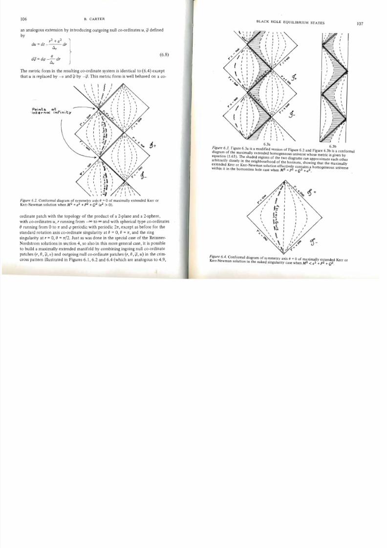
8/7/2019 b carter - equilibrium states of black holes
http://slidepdf.com/reader/full/b-carter-equilibrium-states-of-black-holes 26/48
107106 B. CARTER
an analogous extension by introducing outgoing null co-ordinates u, defined
by
12
r2 + adu =dt---dr
!::.r
a (6.8)d<,{! =d<,{! -- dr
!::.r
The metric form in the resulting co-ordinate system is identical to (6.4) exceptthat u is replaced by -v and ;p by -"$. This metric form is well behaved on a co-
Point:!> a t I
J. i n te rna l inf'ini tyI
I / /d '
"' ' l J ' \ ~ I ,/ I \ \
" , \ \ +I I r \ \
I \
I
Figure 6,2. Conformal diagram of symmetry axis (J = 0 of maximally extended Kerr or
Kerr-Newman solution whenW = 0 2 + p2 + Q2 (0 2
> 0).
ordinate patch with the topology of the product of a 2-plane and a 2-sphere,
with co-ordinates u, r running from _00 to 00 and with spherical type co-ordinates
fi running from 0 to 11 and <,{! periodic with periodic 211, except as before for the
standard rotation axis co-ordinate singularity at fi =0, fi =11, and the ring
singularity at r =0, fi =11/2. Just as was done in the special case of the Reissner
Nordstrom solutions in section 4, so also in this more general case, it is possible
to build a maximally extended manifold by combining ingoing null co-ordinate
patches (r, fi,;P, v) and outgoing null co-ordinate patches (r, fi,"$, u) in the criss
cross pattern illustrated in Figures 6.1, 6.2 and 6.4 (which are analogous to 4.9,
BLACK HOLE EQUILIBRIUM STATES
\ \
\ \ \ \
,\
I
\
\ ~ ~ 1+I \ \,,%
cP j/: \1', I I \
-< :!:J I \ 'cP, I \
I I \
I I 3 J ,,,
\
I
6.3a 6.3b Figure 6.3. Figure 6.3a is a modified version of Figure 6.2 and Figure 6.3b is a conformal diagram of the maximally extended homogeneous universe whose metric is given by
equation (5.63). The shaded regions of the two diagrams can approximate each other
arbitrarily closely in the neighbourhood of the horizons, showing that the maximally
extended Kerr or Kerr-Newman solution effectively contains a homogeneous universe within it in the bottomless hole case when W =p2 + Q2 + 0 2 .
, " \ ~ , ,J~ / 1 : ,,", 05+
'l 1 /< I I \ '
I I \
I, 1;- ,\
\
,I
\
\
, \'I ,, I, I
<\) , , I ,I
, \ I I I i (f'
, '\
, I /1 1 J(
~ / / . . (,;;.
....
Figure 6.4. Conformal diagram of symmetry axis (J = 0 of maximally extended Kerr orKerr-Newman solution in the naked singularity case when W < 02 + p2 + Q2 .
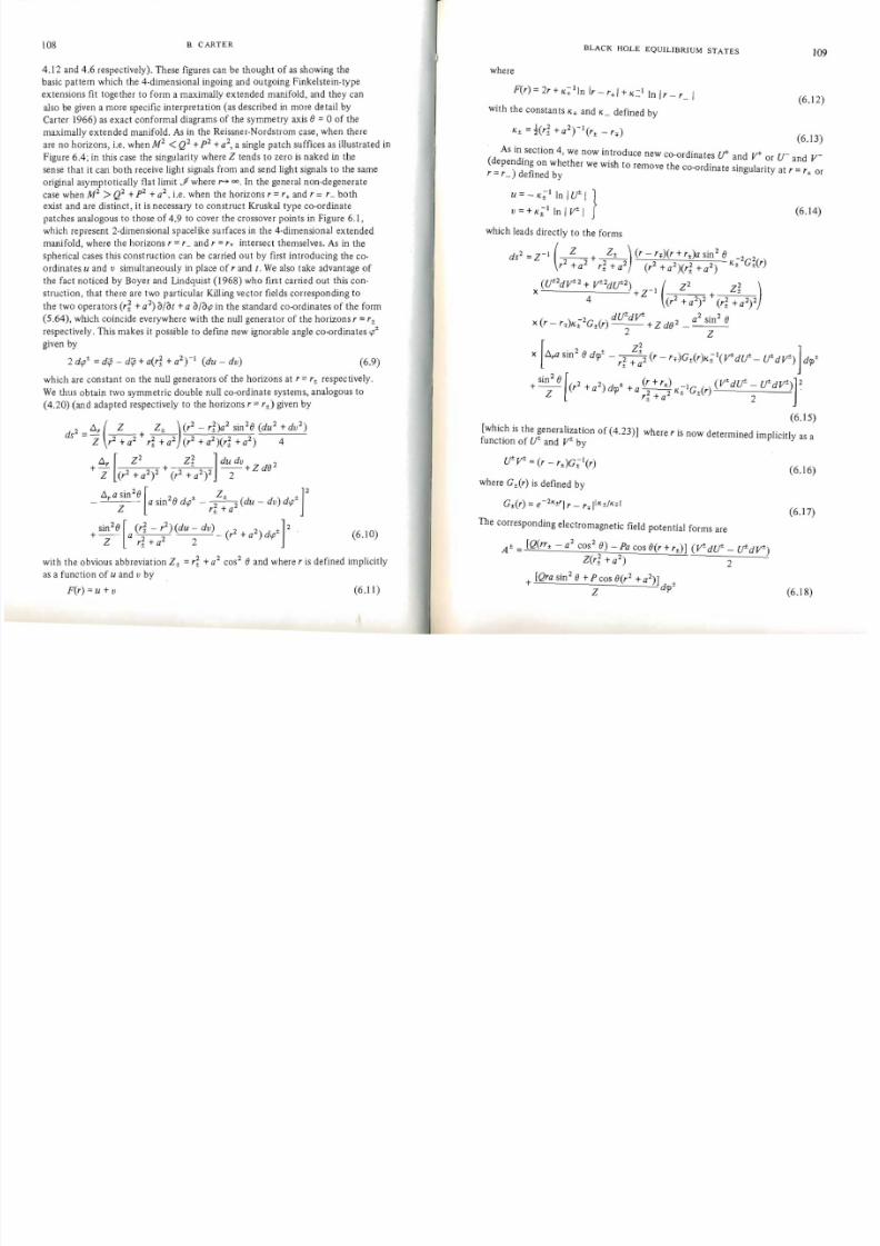
8/7/2019 b carter - equilibrium states of black holes
http://slidepdf.com/reader/full/b-carter-equilibrium-states-of-black-holes 27/48
109108 B. CARTER
4 .12 and 4.6 respectively). These figures can be thought of as showing the
basic pattern which the 4-dimensional ingoing and outgoing Finkelstein-type
extensions fit together to form a maximally extended manifold, and they can
also be given a more specific interpretation (as described in more detail by
Carter 1966) as exact conformal diagrams of the symmetry axis 8 = 0 of the
maximally extended manifold. As in the Reissner-Nordstrom case, when there
are no hOrizons, i.e. when M2 < Q2 + p2 + a2, a single patch suffices as illustrated in
Figure 6.4; in this case the singularity where Z tends to zero is naked in the
sense that it can both receive light signals from and send light signals to the same
original asymptotically flat limit .Jf where In the general non-degenerate00 .
case when M2 > Q2 + p2 +a2, i.e. when the horizons r = r+ and r = r_ both
exist and are distinct, it is necessary to construct Kruskal type co-ordinate
patches analogous to those of 4.9 to cover the crossover points in Figure 6.1,
which represent 2-dimensional spacelike surfaces in the 4-dimensional extended
manifold , where the horizons r = r_ and r = r+ intersect themselves. As in the
spherical cases this construction can be carried out by first introducing the co
ordinates u and v simultaneously in place of rand t. We also take advantage of
the fact noticed by Boyer and Lindquist (I 968) who first carried out this con
struction, that there are two particular Killing vector fields corresponding to2
the two operators ( r ~ + a ) a/at + a a/a.p in the standard co-ordinates of the form
(5 .64), which coincide everywhere with the null generator of the horizons r = r ±
respectively. This makes it possible to define new ignorable angle co-ordinates .p±
given by
2 d.p± = d<jJ - dip + a(r; + a2) - I (du - dv) (6.9)
which are constant on the null generators of the horizons at r =r± respectively.
We thus obtain two symmetric double null co-ordinate systems, analogous to
(4.20) (and adapted respectively to the horizons r = r±) given by
.1 (Z Z+ ) (r2 - r ~ ) a 2 sin28 (du2
+ dv2
)d 2 - r + - -'---:=--7'-' - : ~ - - = - -'--------'
S --Z r2+a 2 r;+a2 (r2+a2)(r;+a2) 4
.1r [Z2 du dv 2
+- + - - - + Z d 8Z (r2 + a2)2 (r2 + a2)2 2
2.1 aSin 8[ · 2 8 d.p-+ Z± - dv) d.p+J2
- r a sm - - 2--2 (du Z r± +a
2sin 8 [ (r ; - r2)(du - dv) (2 2) d ±]2
+-- a 2 2 - r +a .p (6.10)Z r± + a 2
2with the obvious abbreviation Z± = +a cos2 8 and where r is defined implicitly
as a function of u and v by
F(r) =u + v (6.11)
BLACK HOLE EQUILIBRIUM STATES
where
F ( r ) = 2 r + K ~ l l n Ir-r+I+K.::::llnlr _ r_1(6.12)
with the constants K+ and K_ defined by
K± =t(r; +a2)-I(r± -r",)(6.13)
As in section 4, we now introduce new co-ordinates if and v+ or U- and V
(depending on whether we wish to remove the co-ordinate Singularity at r = r+ orr =r_ ) defined by
u = - K;l In Iif I }
(6.14)v = + K± I In I V- I
which leads directly to the forms
2 -I (z Z ± ) (r - r",)(r + r±)a sin2
8 -2 2( )ds =Z - - + - - K+ G+ r2r2+a
2r;+a (r2+a 2)(r;+a 2) -
2 2( i f dV-2 + V- dif2) _ (Z2
x +Z I + ~ _ ~ 4 ~ 2 + a ~ 2 ~ ~ + a ~ 2 2 difdV- 2 a2 sin 2 8x (r - r",)K; G±(r)-2 - +Z d8 _ -
2x [.1,a sin 8 drr/- 2 Z;2 (r - r",)G±(r)K;I(V-dif- i fdV-)]d /qr± + a
2sin 8 [( 2 2) ± (r + r±) -IG () (V-dif - i fdV-)] 2
+-- r +a drp +a---2 K+ + r2Z r± +a - - 2
(6.15)
[which is the generalization of (4.23)] where r is now determined implicitly as a function of if and V- by
if V- = (r - r±)G;tcr)(6.16)
where G±(r) is defined by
G±(r) =e -2k±,Ir _ r", II k ±Ik",I(6.17)
The corresponding electromagnetic field potential forms are
2 2A ± = [Q(rr± - a cos 8) - Pa cos 8(r + r±)] (V-dif _ ifdV-)
Z(r; + a2) 2
[Qra sin2
8 +P cos 8(r2 +a2)] ++ dV
Z (6.18)
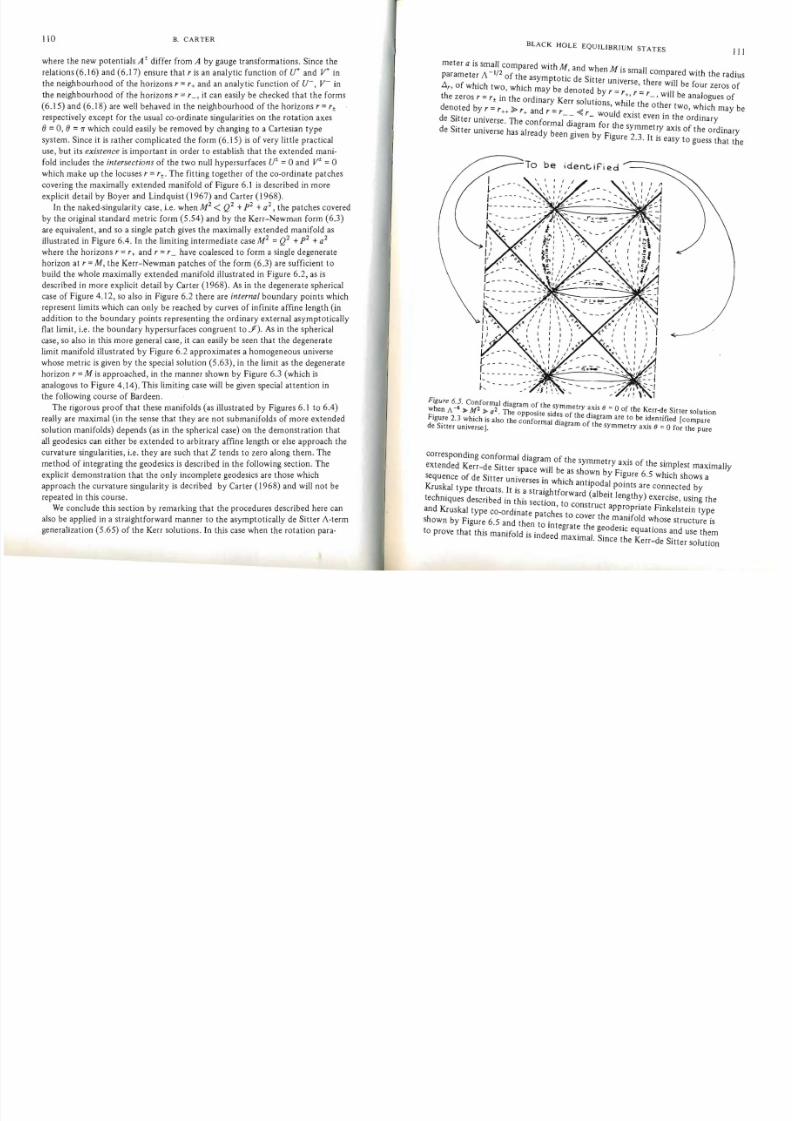
8/7/2019 b carter - equilibrium states of black holes
http://slidepdf.com/reader/full/b-carter-equilibrium-states-of-black-holes 28/48
I I I110 B. CARTER
where the new potentials A ± differ from A by gauge transformations. Since the
relations (6.16) and (6.17) ensure that r is an analytic function of if and v+ in
the neighbourhood of the horizons r = r+ an d an analytic function of U- , V- in
the neighbourhood of the horizons r = r_, it can easily be checked that the forms
(6.15) an d (6.18) are well behaved in the neighbourhood of the horizons r =r±
respectively except for the usual co-ordinate singularities on the rotation axes
e=0, e=1f which could easily be removed by changing to a Cartesian type
system. Since it is rather complicated the form (6.15) is of very little practical
use, bu t its existence is important in order to establish that the extended mani
fold includes th e intersections of the two null hypersurfaces if = 0 and r = 0
which make up the locuses r =r±. Th e fitting together of the co-ordinate patches
covering the maximally extended manifold of Figure 6 .1 is described in more
explicit detail by Boyer and Lindquist (1967) and Carter (1968).
In th e naked-singularity case, i.e. when M2 < Q2 +p2 +a2, the patches covered
by the original standard metric form (5 .54) and by the Kerr-Newman form (6.3)
are equivalent, and so a single patch gives the maximally extended manifold as2illustrated in Figure 6.4 . In the limiting intermediate case M2 = Q2 + p2 +a
where the horizons r = r+ and r = r_ have coalesced to form a single degenerate
horizon at r = M, the Kerr-Newman patches of the form (6.3) are sufficient to
build the whole maximally extended manifold illustrated in Figure 6.2, as is
described in more explicit detail by Carter (1968). As in the degenerate sphericalcase of Figure 4 .12, so also in Figure 6.2 there are internal boundary points which
represent limits which can only be reached by curves of infinite affine length (in
addition to the boundary points representing the ordinary external asymptotically
flat limit , i.e. th e boundary hypersurfaces congruent to f ) . As in the spherical
case, so also in this more general case, it can easily be seen that the degenerate
limit manifold illustrated by Figure 6.2 approximates a homogeneous universe
whose metric is given by the special solution (5.63) , in the limit as the degenerate
horizon r =M is approached, in the manner shown by Figure 6.3 (which is
analogous to Figure 4.14). This limiting case will be given special attention in
th e following course of Bardeen .
Th e rigorous proof that these manifolds (as illustrated by Figures 6.1 to 6.4)
really are maximal (in the sense that they are no t submanifolds of moreextended
solution manifolds) depends (as in the spherical case) on the demonstration that
all geodesics can either be extended to arbitrary affine length or else approach the
curvature singularities, i.e. they are such that Z tends to zero along them. Th e
method of integrating the geodesics is described in the following section . The
explicit demonstration that the only incomplete geodesics are those which
approach the curvature singularity is decribed by Carter (1968) and will not be
repeated in this course.
We conclude this section by remarking that the procedures described here can
also be applied in a straightforward manner to the asymptotically de Sitter A-term
generalization (5 .65) of the Kerr solutions. In this case when the rotation para-
BLACK HOLE EQUILIBRIUM STATES
meter a is small compared with M, and when M is small compared with the radius
parameter 1\ -1/2 of the asymptotic de Sitter universe , there will be four zeros of
Ar, of which two, which may be denoted by r =r+ , r =r_, will be analogues of
the zeros r = r ± in the ordinary Kerr solutions , while the other two, which ma y be
denoted by r = r++ r+ and r = r__ r_ would exist even in the ordinary
de Sitter universe . The conformal diagram for the symmetry axis of the ordinary
de Sitter universe has already been given by Figure 2.3 . It is easy to guess that the
To be ident. iF'i ed
corresponding conformal diagram of the symmetry axis of the simplest maximally
extended Kerr-de Sitter space will be as shown by Figure 6.5 which shows a
sequence of de Sitter universes in which antipodal points are connected by
Kruskal type throats. It is a straightforward (albeit lengthy) exercise, using the
techniques described in this section , to construct appropriate Finkelstein type
and Kruskal type co-ordinate patches to cover the manifold whose structure is
shown by Figure 6.5 and then to integrate the geodesic equations and USe them
to prove that this manifold is indeed maximal. Since the Kerr-de Sitter solution
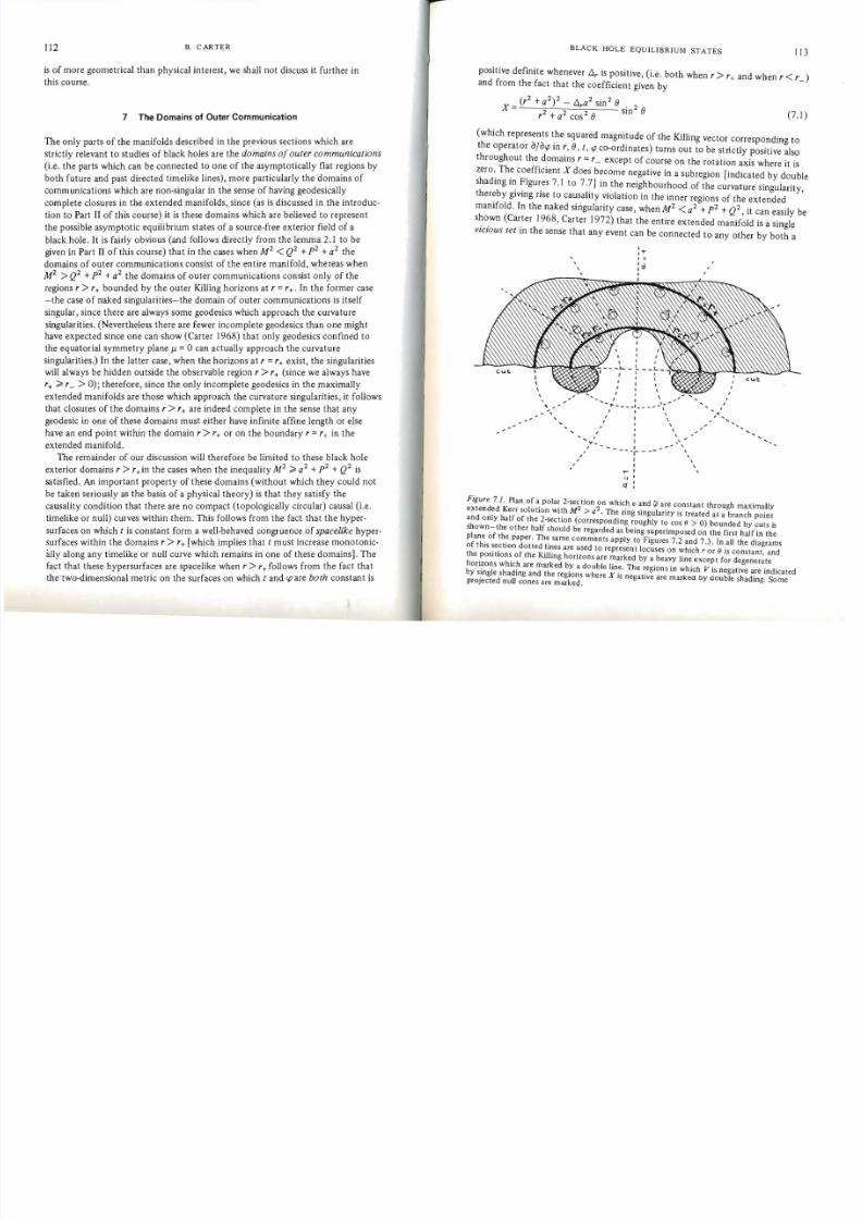
8/7/2019 b carter - equilibrium states of black holes
http://slidepdf.com/reader/full/b-carter-equilibrium-states-of-black-holes 29/48
7
113112 B. CARTER
is of more geometrical than physical interest, we shall not discuss it further in
this course.
The Domains of O uter Communication
The only parts of the manifolds described in the previous sections which are
strictly relevant to studies of black holes are the domains o[ oute, communications
(i.e. the parts which can be connected to one of the asymptotically flat regions by
both future and past directed timeJike lines), more particularly the domains of
communications which are non-singular in the sense of having geodesically
complete closures in the extended manifolds, since (as is discussed in the introduc
tion to Part II of this course) it is these domains which are believed to represent
the possIble asymptotic equilibrium states of a source-free exterior field of a
black hole. It is fairly obvious (and follows directly from the lemma 2.1 to be
given in Part II of this course) that in the cases when M2 < Q2 + p2 +a2 the
domains of outer communications consist of the entire manifold, whereas when
M2 >Q2 + p2 +a2 the domains of outer communications consist only of the
regions, >'+ bounded by the outer Killing horizons a t , ='+. In the former case
-the case of naked singularities-the domain of outer communications is itself
singular, since there are always some geodesics which approach the curvature
singularities. (Nevertheless there are fewer incomplete geodesics than one might
have expected since one can show (Carter 1968) that only geodesics confined to
the equatorial symmetry plane J1 = 0 can actually approach the curvature
Singularities.) In the latter case, when the horizons a t , ='+ exist, the singularities
will always be hidden outside the obstrvable region, >'+ (since we always have
'+ ;;" _> 0); therefore, since the only incomplete geodesics in the maximally
extended manifolds are those which approach the curvature singularities, it follows
that closures of the domains, >'+ are indeed complete in the sense that any
geodesic in one of these domains must either have infinite affine length or else
have an end point within the domain, >'+ or on the boundary,='+ in the
extended manifold.
The remainder of our discussion will therefore be limited to these black holeexterior domains, > ,+ in the cases when the inequality M2 ;;, a2 + p2 + Q2 is
satisfied. An important property of these domains (without which they could not
be taken seriously as the basis of a physical theory) is that they satisfy the
causality condition that there are no compact (topologically Circular) causal (i.e.
timelike or null) curves within them. This follows from the fact that the hyper
surfaces on which t is constant form a well-behaved congruence of spacelike hyper
surfaces within the domains, > ,+ [which implies that t must increase monotonic
aJly along any timelike or null curve which remains in one of these domains). The
fact that these hypersurfaces are spacelike when' >'+ follows from the fact that
the two-dimensional metric on the surfaces on which t and </) are both constant is
BLACK HOLE EQUILIBRIUM STATES
positive definite whenever I1r is positive, (i.e. both when, > ,+ and when, <,_)and from the fact that the coefficient given by
(,2 + a2)2 _ 11 a2 sin2 (J
X = r sin2 (J, 2 + a2 cos 2 (J (7.1)
(which represents the squared magnitude of the Killing vector corresponding to
the operator a/a</) in " (J, t, </) co-ordinates) turns out to be strictly positive also
throughout the domains, =,_except of course on the rotation axis where it iszero. The coefficient X does become negative in a subregion [indicated by double
shading in Figures 7.1 to 7.7) in the neighbourhood of the curvature singularity,
thereby giving rise to causality violation in the inner regions of the extended
manifold. In the naked singularity case, when M2 < a2 + p2 + Q2, it can easily be
shown (Carter 1968, Carter 1972) that the entire extended manifold is a single
vicious set in the sense that any event can be connected to any other by both a
,, .....
, , ", ,
,
I
I, I
II \
I// I I \ ......I....... . . . . . - _I .. ___ ... \
I, ,
, I\
\I
I, "
v " /
I " ,I
-----}---I
.,..
::$."
Figure 7.1. Plan of a polar 2-section on which u and tp are constant through maximally2
extended Kerr solu"tion with W > 0 . The ring singularity is treated as a branch point
and only half of the 2-section (corresponding roughly to cos e > 0) bounded by cuts is
shown-the other half should be regarded as being superimposed on the first half in the
plane of the paper. The same comments apply to Figures 7.2 and 7.3. In all the diagramsof this section dotted lines are used to represent locuses on which r or e is constant, andthe positions of the Killing horizons are mar ked by a heavy line except for degenerate
horizons which are marked by a double line. The regions in which V is negative are indicatedby single shading and the regions where X is negative are marked by double shading. Someprojected n uti cones are marked.

8/7/2019 b carter - equilibrium states of black holes
http://slidepdf.com/reader/full/b-carter-equilibrium-states-of-black-holes 30/48
---
114BLACK HOLE EQUILIBRIUM STATES lISB. CARTER
,,'
I
""
-. L • ,,",,'",I
- - -.-
I
- - , I, ,. , , ,, , ..\ ,
\ ,,, \\
-{" - - - -.---- ...... ...
,, I \
,, ,1 \
\
, .,-' \,, "I '
=1' \ \ Figure 7.4. Rough sketch in perspective of a polar 2-section in which v and are constant
through a maximally extended Kerr solution when > a2 (this is an alternative representaFigure 7.2. Plan of polar 2-section in which v and are constant through a maximallY ex
tion of the same section as is shown in Figure 7.1).2
tended Kerr solution in the degenerate case when M2 =a .
T '.. ' ,,
, , ," ,
, - --:- - ..., ,, , ,, ,..- , ' > ~ ,,, , ,, ,,
1 -, , ---.-_ ... .,.. , ,,, 1
" '";i '
Figure 7.5. Rough sketch in perspective of a polar 2-section in which v and are constantFigure 7.3. Plan of a polar 2-section in which v and;P are constant through a maximallythrough a maximally extended Kerr-Newman solution when > a2 + p2 + Q2. .
extended Kerr solution when < a2
117BLACK HOLE EQUILIBRIUM STATES
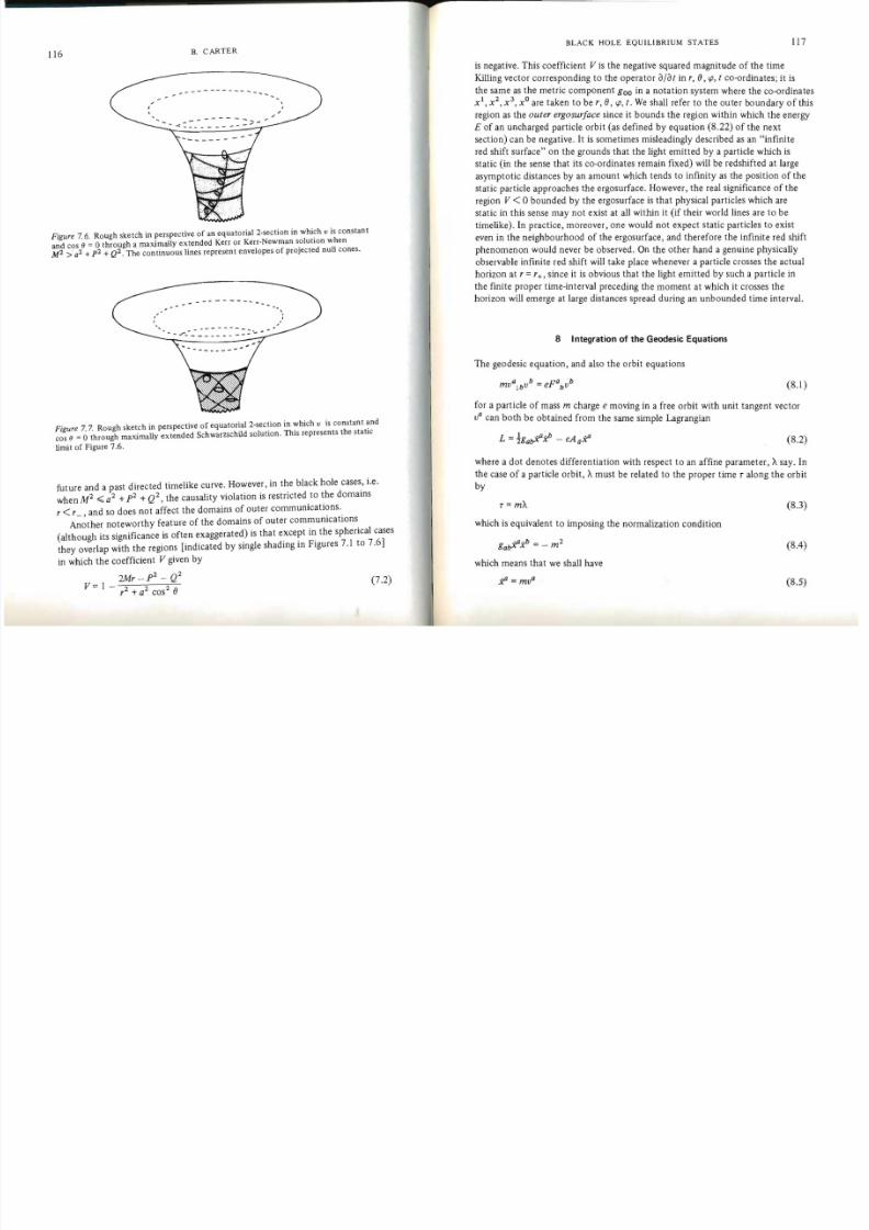
8/7/2019 b carter - equilibrium states of black holes
http://slidepdf.com/reader/full/b-carter-equilibrium-states-of-black-holes 31/48
116 B. C ARTER
. ,
Figure "7.6. Rough sketch in perspective of an equatorial 2-section in which u is constantand cos e = 0 through a maximally extended Kerr or Kerr-Newman solution whenM'2 >'0 2 + p2 + Q2 . The continuous lines represent envelopes of projected null cones.
Figure 7. 7. Rough sketch in perspective of equatorial 2-section in which u is constant andcos e = 0 through maximally extended Schwarzschild solution. This represents the static
limit of Figure 7.6.
future and a past directed timelike curve . However, in the black hole cases, i.e.
when M2 .;;;; a2 +p2 + Q2 , the causality violation is restricted to the domains
r < r _ , and so does not affect the domains of outer communications .
Another noteworthy feature of the domains of outer communications
(although its significance is often exaggerated) is that except in the spherical cases
they overlap with the regions [indicated by single shading in Figures 7.1 to 7.6]
in which the coefficient V given by
2Mr _ p2 _ Q2V= 1 _ (7 .2)
r2 +a2 cos
2 e
is negative. This coefficient V is the negative squared magnitude of the time
Killing vector corresponding to the operator arot in r, e, cp, t co-ordinates; it is
the same as the metric component goo in a notation system where the co-ordinates
X l, x 2, x 3
, xO are taken to be r, e, cp, t . We shall refer to the outer boundary of this
region as the ou ter ergosurface since it bounds the region within which the energy
E of an uncharged particle orbit (as defined by equation (8.22) of the next
section) can be negative. It is sometimes misleadingly described as an "infinite
red shift surface" on the grounds that the light emitted by a particle which is
static (in the sense that its co-ordinates remain fixed) will be redshifted at large
asymptotic distances by an amount which tends to infinity as the position of the
static particle approaches the ergosurface. However, the real significance of the
region V < 0 bounded by the ergosurface is that physical particles which are
static in this sense may not exist at all within it (if their world lines are to be
timelike). In practice, moreover, one would not expect static particles to exist
even in the neighbou rhood of the ergosurface, and therefore the infinite red shift
phenomenon would never be observed. On the other hand a genuine physically
observable infinite red shift will take place whenever a particle crosses the actual
horizon at r = r+, since it is obvious that the light emitted by such a particle in
the finite proper time-interval preceding the moment at which it crosses the
horizon will emerge at large distances spread during an unbounded time interval.
8 Integration of the Geodesic Equations
The geodesic equation, and also the orbit equations
mva;bVb =eFOb,} (8.l)
for a particle of mass m charge e moving in a free orbit with unit tangent vector
va can both be obtained from the same simple Lagrangian
L = t g a ~ . x b - eAoXO (8.2)
where a dot denotes differentiation with respect to an affine parameter, Asay. Inthe case of a particle orbit, Amust be related to the proper time T along the orbit
by
T= mA (8.3)
which is equivalent to imposing the normalization condition
2g a ~ x b = _ m (8.4)
which means that we shall have
aXO =mv (8 .5)
118 B. CARTER

8/7/2019 b carter - equilibrium states of black holes
http://slidepdf.com/reader/full/b-carter-equilibrium-states-of-black-holes 32/48
The geodesic equations are obtained from the Lagrangian (8.2) when e is set
equal to zero .
Introducing the mome ntum co-vector
Pa=gabAb-eA a (8.6)
we see that the Hamiltonian co rresponding to the Lagrangian (8.2) has the very
simple form
H =-!t'b(pa + eAa)(Pb + eA b) (8.7)
Since th e affine parameter Adoes not appear explicitly in the Hamiltonian, the
Hamilton ian itself will automatically be a co nstant of the motion , and by the
normalization condition (8.4) it is clear that this constant is given simply by
H= _-!m2
(8.8)
\\'hen one of the co-ordinates, x O say, is ignorable (i.e. does not appear explicitly
in the Hamiltonian) the corresponding momentum Po will commute with the
Hamiltonian (in the sense that its Poisson bracket with the Hamiltonian will be
zero) and hence it will also be a constant of the motion . In the case of the metric
form (5 .18) with the electromagnetic field potential (5.45) there are tw oindependent ignorable co -ordinates, namely t and tp and hence th e co rresponding
momen ta Pt and Pop will both be conserved, giving two co nstants of the motion in
addition to the constant given by (8.7) which would always exist.
To obtain a complete set of explicit first integrals of the motion we need to
have a fourth constant of the motion. In a general stationary-axisymmetricspace
time an independent fourth integral would not exist, but the condition that the
charged Klein Gordon equation be separable (which we imposed in our derivation
of the Kerr solutions) automatically guarantees the weaker condition that the
Hamilton-Jacobi equation corresponding to th e Hamiltonian (8.6) will be
separable in the pre se nt case (Carter 1968a, Carter 1968 b), thus ensuring the
existence of the required fourth integral. We shall not use the Hamilton-Jacobi
formalism in the present section, but instead shall show how the fourth co nstantmay be obtained directly by inspect ion of the Hamiltonian using the following
lemma:
LEMMA Let the Hamiltonian have th e form
I Hr +HIl(8.9)
H=2U +Ur Il
where Ur and U are single variable functions of the co-ordinates rand JJ. respecll
tively and where Hr is independent of the momentum PIl and of all the co
ordinate functions other than r, and H11 is independent of the momentum Pr and
BLACK HOLE EQUILIBRIUM STATES 119
of all th e co-ordinate fun ctions other than JJ.. Then the quantity
K=UrH Il - UIlHr(8.10)Ur + U
ll
commutes with H and hence is a constant of the motion.
Proo f Since the stipulated conditions clearly ensure that Hr commutes with
HIl , and since HIl naturally co mmutes with itself, we obtain
[H"HJ =-!(Hr+HIJ) [H" I ] (8.11)Ur + UIJ
Similarly since Ur clearly commutes with HIJ and with Ur + U we obtainll
I(8.12)[U"HJ =2(U +U ) [Ur , HrJ
r IJ
Working out the Poisson brackets on the right hand sides we find
I ] I aHrdUr[Hr, Ur +·UIJ = - (Ur + UIJ)2 apr &
I (8.13)(U + UIJ)2 [Ur' HrJr
Thus we can eliminate the right hand sides of (8.11) and (8.12) to obtain
[Hr, HJ =2H[U" HJ (8.14)
It follows immediately that th e quantity
K= 2UrH -Hr (8.15)
commutes with H an d hence is a constant of the motion . It is clear from (9.8)
that this quantity K can also be expressed in the form
K =HIJ - 2UIlH (8.16)
and also in the more symmetric form (8.10). This co mpletes the proof.
Now the Hamiltonian co rresponding to our canonical separable metric form
(5.18) with the canonical vector potential (5.45) can be read off directly from the
inverse metric (5.16) as
H = t : : . / l P ~ + t::.;I[C/:!p op +ZIlPt- eX/:!f
2 ( C ~ r - CrZIl)
+ t : : . r P ~ - t::.;1 [CrPr +Z/lPt + eXrf(8.17)
2 ( C ~ r - CrZIJ)
120 B. CARTER
8/7/2019 b carter - equilibrium states of black holes
http://slidepdf.com/reader/full/b-carter-equilibrium-states-of-black-holes 33/48
121
which clearly has the form (8.9) with
Hr =6.rP; - 6.;1 [CrP.p + ZrPt + eXr]2 (8 .18)
HIJ = 6 . I J P ~ + 6 . ~ I [ C I J P I J + ZIJPt- eXIJ]2 (8.19)
Ur = C ~ r (8.20)
(8 .21)UIJ = -CrZlJ
It follows at once from the lemma that there will indeed be a fourth constant of
the motion K given equivalen tly by (8.10) or (8.16) in terms of the expressions(8.18), (8.19), (8.20), (8.21), in addition to the constant H given by (8.17) and
the energy and polar angular momentum constants £ and L z given by
(8.22)£= -P t
L z =p.. (8.23)
In terms of the actual source free solutions (5.46) to (5.53) we shall have
H = ( l _ p 2 ) p ~ + ( I _p2)-I[p.p+a(l_p2)pt_ ePp]2
2(r2 +a2p2)
+ 6.rP; - 6.;1 [ap.p + (r2 + a2)pt + eQr]2
(8.24)2(r2 +a2p2)
and the corresponding expression for K will be
K =a2(J - p2){6.rP; - 6.;1 [ap.p + (r2 + a2)pt+ eQr]2}
r2 +a 2p2
+(r2 + a2){(1 - p 2 ) p ~ + (I - p2)-I[p.p + aO - p2)pt - ePp]2}
r2 +a2p2
(8.25)
where 6.r is given by (5.52).
Transforming from momentu m to velocity co-ordinates and setting p = cos ewe obtain the four constants of the motion explicitly as two linear combinations
(r2 _ 2Mr + a2 cos2 e + p2 + Q2)i£ = ~ - - - - = - - . . . " . - - . , . . . - - - - ' = - : ' " 2 2r2 +a cos e
(2Mr - p2 - Q2)a sin2 + e(Qr +aPp) + ~ - - - ~ ~ ~ - ~ - ~ - - ~ (8.26)r2 +a2 cos2 e
[(r2 +a2)2 - 6.rG2 sin2 e] sin2 L = ~ - ~ - - - - = - - - - ' ~ - - = - ~ - - ' -z r2 +a2 cos2 e
-(2Mr - p2 _ Q2)a sin 2 e i + e[aQr sin2 e + p(r2 + ~ ) cos e]+ ~ - - - - - - ~ ~ - - ~ ~ - - - - ~ - - - - ' - - ~ (8.27)2 2er2 +a cos
BLACK HOLE EQUILIBRIUM STATES
and two quadratic combinations
2m =_(r2 + a 2 c o s 2 e ) ( ~ : +IF)
2sin e 2 2 · . 2 6.r 2 . . 2
2 2 2 [(r +a ).,0- at] + 2 2 2 [a sin 8.,0 - t]r +a cos 8 r +a cos 8
(8.28)
A2 2 r2 +a2 co s28 ·2 U 2 . . }r
K=a sin 8 r - 2 2 2 [asin 8.,o-t]2( 6.r r +a cos 8
+ (r2 + a2) {(r
2+ a
2COS
2e)(P + 2 S i ~ 2 8 2 [(r2 + a 2 ) ~ - aW}r + a cos 8
(8.29)
Introducing the functions
R(r) = [£(r2 +a2) - aL z - eQr]2 -; 6.r(m2r2 +K) (8.30)
8(8)=K-m2a
2cos
28 - sin-
28[£asin
28 -Lz+ePcos8]2 (8.31)
= C+ 2aeP£ cos 8 + [a2(£2 - m2)_(L; + e2p2)sin-2 8]cos28 (8.32)
where C is a constant given in terms of K by
C = K - (L - a£)2z (8.33)
we can express the non·ignorable co-ordinate velocities by the equations
Z2;.2 = R(r) (8.34)
Z262 =8(8) (8.35)
It is clear from the form of (8 .35) and (8.31) that K must always be positive if 6is to be real. The ignorable co-ordinate velocities can be expressed directly as
2=L [_ ._12- _ a ] _ a£(2Mr - p2 - Q2) (8.36)
z
Si n e 6.r 6.r 2 2
. [(r +a )2 . ] (2Mr _ p2 _ Q2)Zt =£ - a2
Si n 2 8 - aL -'---_--'::....-'. (8.37)6.r z 6.r
Hence we can obtain the final fully integrated form of the orbit equations as
J6
de Jr
drve= y IR (8.38)
6 r2
COS2 8 d8 Jr2 drA= J
a+ -- (8.39)
VB VR
123122 B. CARTER BLACK HOLE EQUILIBRIUM STATES

8/7/2019 b carter - equilibrium states of black holes
http://slidepdf.com/reader/full/b-carter-equilibrium-states-of-black-holes 34/48
f, e
fLZ +a£(2Mr - p2 - Q2)] dr f L z dU
~ = + + ---- (8.40)/:::,..,V'R. sin2 eve
, e2 2 2
t =+f [£(r2 + a )2 - aLzC2Mr - p2 - Q2)]dr -f a £sin e de(8.41 )
/:::,..,VR ve
Applications of these equations are discussed in the following course by Bardeen.
We conclude by remarking that the linear constants of the motion £ and L z
can be expressed in the form
£ = -k"Pa (8.42)
and
=mapa (8.43)L z
in terms of the Killing vector components k" and ma defined by
k" (8.44)ax
a
at
a a a-= m - (8.45)
axa
It can easily be seen that the Killing equations
k(a;b) = 0 (8.46)
m(a;b) = 0 (8.4 7)
are both necessary and suffici ent for £ and L z as defined by (8.42) and (8.43) to
be constant along all geodesics. In order for them to be constant along charged
particle orbits as well it is further necessary and sufficient that the invariance
conditions
Aaka;b +Ab ;ak" = 0 (8.48)
Aama;b+Ab;ama = 0 (8.49)
be satisfied, as they are in the presen t case.
Now the quadratic constant of the motion (8.29) can analogously be expressed
in the form
. a . bK = aatJX X (8.50)
where aab is a symmetric tensor given by
22 a sin2 edr
2]
aab dxadx
b= (r2 + a cos
2e) [
/:::,.., + (r2 + a2) de 2
(r2 +a2) sin2 e [(r2 +a2) - a dt]2+ ~ - - ~ ~ ~ ~ - ~ ~ - - ~2r2 +a cos2 e /:::"',a
2 sin2 e [a sin2 e - dt]2 (8.51 )
r2+
a2
cos2
e[This expression (8.50) for K having a similar form to the expression (8.4) for the
constant m2.] It is a standard result (see Eisenhart 1926) that the equations
a(ab;c) = 0 (8.52)
are both necessary and sufficient for an expression of the form (8 .50) to be
constant along all geodesics. Since the equation (8.52) is analogous to the Killing
equations (8.46) which are necessary and sufficient for the analogous linear
expression to be constant along geodesics, Penrose and Walker (1969) in a recent
discussion have introduced the term Killing tensor to describe a symmetric tensor
satisfying the equat ions (8.52). Personally I would prefer to call it a Stackel tensor
since Stackel (a contemporary of Killing) actually made the first studies of the
kind of Hamilton-Jacobi separability which gives rise to the existence of such a
tensor (Stackel 1893).
It is to be noted that the existence of the Stackel-Killing tensor is not in itself
sufficient to ensure that the quadratic expression (8.50) is constant along charged
particle orbits as well as geodesics. It is easy to see that in general a necessary and
sufficient condition for the quadratic expression aaaXaxb to be constant along
charged particle orbits is that in addition to (8 .52) the electromagnetic field
should be such that
a a ( ~ C ) a =0 (8 .53)
It is clear that in any space the metric tensor gab will satisfy the Stackel-Killing
equations (8.52) and also that it will satisfy the condition (8.53) for arbitrary
Fab , thus giving rise to the constant of motion (8.4). Also when there at:..e Killing
vectors present their symmetrized products also form Stackel-Killing tensors, so
that in the Kerr metrics there is actually a five parameter family of Stackel-Killing
tensors of which five linearly independent members may be taken to be gab, the
tensor aab defined by (8.51), together with k(akb)' k(amb) and m(amb)' These give
rise to five linearly independent constants of which of course only four are
algebraically independent.
The approach to the Kerr metrics which we have adopted here is to start with
the separability properties as a fundamental postulate , and then to derive other
basic algebraic properties such that the fact that the Weyl tensor is of Petrov
124 B. CARTER
8/7/2019 b carter - equilibrium states of black holes
http://slidepdf.com/reader/full/b-carter-equilibrium-states-of-black-holes 35/48
type D. The more traditional approach has been to start from the Petrov type D
property and then to derive the separability properties. The investigations initiated
by Penrose and Walker (1969) are aimed at deriving the separability properties
directly from the Petrov type D property without actually going through the
explicit solution of the field equations. [It is to be emphasized however that the
direct derivation of the existence of the Stackel-Killing tensor can only be an
intermediate stage in this programme, and is by no means sufficient to establish
the full separability properties of the Kerr metrics: there is at present no known
way of deducing the separability of the wave equation-as opposed merely to the
separability of the Hamilton-Jacobi equation-from the Stackel-Killing tensoL]
Some important recent work by Teukolsky (1972) has shown that the Kerr metrics
possess even stronger separability properties than those we have used in the
present course, by which higher spin wave equations (as well as the ordinary
scalar wave equation) can be at least partially separated by combining the
separation methods described at the beginning of section 5 with Petrov-type
analysis. This discovery is likely to prove to be of very great value in future
perturbation analyses of the Kerr solutions.
Bibliography
Bertotti, B. (1959) Phys. Rev. 116, 133l.
Boyer, R. H. and Price, T. G. (1965) Proc. Camb. Phil. Soc. 61, 53l.
Boyer, R. H. and Lindquist, R. W. (1967) 1. Math. Phys. 8,265.
Carter, B. (1966a) Phys. Rev. 141,1242.
Carter, B. (1966b) Physics Letters 21, 423.
Carter, B. (l968a)Phys. Rev. 174, 1559.Carter, B. (1968b) Commun. Math. Phys. 10, 280.Carter, B. (1969) 1. Math. Phys. 10,70.
Debever, R. (1969) Bull. Akad . Roy. de Belgique 55, 8.
Eisenhart, L. P. (1926) Riemmannian Geometry (Princeton)
Finhelstein, D. (1958) Phys. Rev. 110,965.
Graves, J. C. and Brill, D. R. (1960) Phys. Rev. 120,1507.
Goldberg, J. N. and Sachs, R. K. (1962) Acta Phys. Polan. 13. Hughston, L. P., Penrose, R., Sommers, P. and Walker, M. (1972) Commun Math. Phys.27,
303.
Kerr, R. P. (1963) Phys. Rev. Letters 11, 238. Kerr, R. P. and Schild, A. (1964) Am. Math. Soc. Symposium. Kundt, W. and Trumper, M. (1962) Akad. Wiss. Lit. Mainz 12. Lemaitre, G. E. (1933) Am . Soc. Scient. Bruxelles, As3, 5l.
Misner, C. (1963) 1. Math. Phys. 4,924.
Robinson, I. (1959) Bull. Akad. Pol. 7, 35l.
Schwarzschild, K. (1916) BerL Ber. 189. Stachel(1893) Compt. RendusAcad. Sci. 116.1284.
Teukolski, S. A. (1972) preprint Caltech. Walker, M. and Penrose, R. (1970) Commun. Math. Phys. 18,265.
PART II General Theory of
Stationary Black Hole States
1 Introduction
The necessity of facing up to the problem of catastrophic gravitational collapse in
astrophysics was first appreciated by Chandrasekhar in 1931 when he discovered
the upper mass limit for a spherical equilibrium configuration of a cold sphere of
ordinary degenerate matter in Newtonian gravitational theory. Subsequent work
by Chandrasekhar, Landau, Oppenheimer and others established fairly clearly by
the end of the nineteen thirties that the upper mass limit would not be greatly
affected by taking into account the existence of exotic forms of high density
matter, such as a degenerate neutron fluid, nor by the corrections resulting from
the use of Einstein's theory of gravity, according to which an object . , ! i : J ~ J h ili IEit rn.llHultimately disappear from sight within its Schwarzschild horizon-which
occurs when the circumferential radius r is diminished to twice the conserved
mass M (where here, as throughout this work, we use units in which Newton'sconstant G and the speed of light c are set equal to unity)-with the subsequent
formation of a singularity.
It is true of course that an arbitrarily large mass can exist in quasi-equilibrium
in a suffiCiently extended differentially rotating disc-like configuration. However,
it would be rather surprising if nature contrived to avoid the formation of at least
some large stars wit h sufficiently small angular momentum for its effects to be
negligible even after contraction to the Schwarzschild radius. Moreover there are
many diverse effects (including viscosity, magnetic fields, and gravitational radia
tion) which would all tend to transfer angular momentum outwards, except in the
special case of uniformly rotating axially symmetric configurations, for which
there is in any case an upper mass limit, somewhat larger than the spherical upper
mass limit, but of the same order of magnitude. (See for example the work of
Ostriker et al.) Hence although its onset may in some cases be postponed or
prevented, the basic issue of catastrophic collapse cannot be avoided merely by
taking into account natural deviations from spherical symmetry.
Despite these considerations there was very little work in the field until the
mid nineteen-sixties. The first signs of renewed interest were a pioneering attempt
by Regge and Wheeler (1957) to determine the stability of the Schwarzschild
horizon, and an equally important pioneering work by Lifshitz and Khalatnikov
(1961) in which it was suggested that the ultimate singularity which occurs in the
spherical collapse case might be avoided in more general situations. These two
works forshadowed the subsequent subdivision of the field of gravitational collapse
125
126 B. CARTER BLACK HOLE EQUILIBRIUM STATES

8/7/2019 b carter - equilibrium states of black holes
http://slidepdf.com/reader/full/b-carter-equilibrium-states-of-black-holes 36/48
127
investigations into two main branches, the first-with which we shall be concerned
here-being concerned primarily with horizons and astronomically observable
effects, and the second being primarily concerned with the fundamental physical
question of the nature of the singularities and the breakdown of the classical
Einstein theory. Another event which was of key importance in stimulating
interest in the field was the accidental discovery b y Kerr (1963) of a rotating
generalization of the spherical Schwarzschild solut ion of Einstein's vacuum
equations-accidental in the sense that Kerr's investigations were not directly
motivated by the astrophysical collapse problem.
However, the event which laid the foundations of the modern mathematical
theory of gravitational collapse was the publication by Penrose (1965) of the
now famous singularity theorem which conclusively refuted the suggestion that
singularities are merely a consequence of the spherical idealization used in the
early work. The actual conclusion of the Penrose theorem was rather restricted,
being essentially negative in nature , and although its range of application has been
very greatly extended by the subsequent work of Stephen Hawking, there is so far
very little positive information about the nature of the singularities whose
existence is predicted. The real importance of the Penrose theorem lay rather in
the wealth of new techniques and concepts which were introduced in its proof,
particularly the notion of a trapped surface and the idea of treating boundary
horizons as dynamic entities in their own right. These developments lead directlyto the realization that the outcome of a gravitational collapse-in so far as it can
be followed up in terms of the classical Einstein theory-would have to be either
(a) the formation of a well behaved event horizon separating a well behaved
domain of outer communication (within which light signals can no t only be
received from but also sent to arbitrarily large distances) from hidden regions (for
which the term black holes was subsequently introduced by Wheeler) within
which the singularities would be located, and from which no light could escape to
large distances, or (b) the formation of what have come to be known as naked
singularities, i.e. singularities which can be approached arbitrarily closely by time·
like curves or light rays which subsequently escape to infinity. If the latter situation
were indeed to occur it would mean that the classical Einstein theory would be
essentially useless for predicting the subsequent astronomically observablephenomena , so that the development of a more sophisticated gravitational theory
would be an urgent practical necessity. However there are a number of features
of the situation as we understand it at present which encourage belief in the
conjecture which Penrose has termed the cosmic censorship hypothesis , which
postulates that naked singularities do not in fact occur , i.e. that the only possible
outcome of a gravitational collapse is the formation of black holes. It is probably
fair to say that the verification or refutation of this conjecture is the most
important unresolved mathematical problem in General Relativity theory today.
If the cosmic censorship conjectur e is correct then there will be no theoretical
reason wh y Einstein's theory of gravity should no t be adequate for all foreseeable
astronomical purposes, except for dealing with primordial singularities (sometimes
referred to as white holes) such as the cosmological big bang. (It will still of
course be possible that the theory may fail empirically by conflict with observation.)
Having arrived at the idea of a black hole as a possible outcome, if not an in
evitable outcome, of a gravitational collapse, it is natural to conjecture that it
should settle down asymptotically in time towards a stationary final equilibrium
state-any oscillations being damped ou t by gravitational radiation- as indicated
in Figure I. It was after all the non-existence of such a stationary final equilibrium
state for an ordinary massive star which led to the introduction of the alternative
black hole concept in the first place. With these considerations in mind, and the
recently discovered Kerr solution as an example, several workers including myself,
and notably Bob Boyer, began a systematic study of the properties of stationary
black hole states during the years 1965-1966. Too much concentration on the
stationary equilibrium states could not of Course have been justified if the settling
down process took place over astronomically long timescales, but it has sub
sequently become fairly clear from the dynamical perturbation investigationsof
the Schwarzschild solution by Doroshkeviteh, Zel'dovich and Novikov (1966),
Vishveshwara (1970) , Price (1972) and others that (as was suspected, by dimen
sional considerations, from the outset) any dynamic variations of a black hole can
be expected to die away over timescales of the order of the time for light to cross
a distance equal to the Schwarzschild radius. These timescales are in fact extremely
short by astronomical timescales-of the order of milliseconds for the collapse of
an ordinary massive star, and at most hours or days for the collapse of an entiregalactic nucleus.
This early work served to clarify many of the elementary properties of the
black hole event horizons in the stationary case, and also their relationship with
other geometrically defined features such as what has subsequently come to be
known as the ergosurface, which are described in detail in sections 2 to 5. This
phase of elementary investigation was almost complete by the time of Boyer's
tragic death in the summer of 1966, although the results were not actually
pUblished until somewhat later, (Boyer (1969), Carter (1969), Vishveshwara
(1968)). The results described in section 8 were overlooked in this earlier period
and were obtained quite recently (by Hartle, Hawking and myself) while therigorous proofs in section 9 were actually worked ou t at Les Houches by Bardeen,Hawking and myself.
An analogous first phase of investigationof the elementary properties of black
hole even horizons in the more general dynamic case has been carried out more
recently almost exclusively by Stephen Hawking, using some of the techniques
developed by Penrose, Geroch and himself for proving Singularity theorems ; the
most important of these elementary properties is that the area of the intersection
of a constant time hypersurface with the event horizon (which is of COurse
constant in the stationary case) can only increase but never decrease with time in
the dynamic case (Hawking 1971). An off.shoot of this work has been a much
more sophisticated second phase of investigations of stationary black hole event
128129
B. CARTERBLACK HOLE EQUILIBRIUM STATES

8/7/2019 b carter - equilibrium states of black holes
http://slidepdf.com/reader/full/b-carter-equilibrium-states-of-black-holes 37/48
N Pole
5 pole
Figure 2. Equatorial and polar sections of a conceivable axially and equatorially symmetricgalactic nucleus are illustrated., The nucleus is supposed to consist of a stellar system (whose
intersections with the equatorial and polar planes are represented by the shaded regions)with a massive central black hole. (The hole will be non-Kerr-like due to the distortinginfluence of the stellar mass distribution.) Projections onto the equatorial and polar planesof two stellar orbits (related by a 90 degree axisymmetry rotation) are marked, using dotted
lines where the orbits lie behind the relevant planes. These would be typical orbits in asystem which is approximately stationary (in that mass redistribution as the stars fall into
the hole takes place over timescales long compared with the orbital periods) bu t in whichthe circularity condition is violated due to a ne t inflow of matter at high latitudes compensated by a net outflow near the equator. (In order to obtain this circularity violation
it is necessary not only that the orbits be eccentric bu t also that they should have aconsistent average tilt.) The Papapetro.u theorem is sufficiently powerful to ensure that thespacetime will be stationary-circular' in the empty region in the neighbourhood of the hole
despite the non-circularity resulting from the quasi-convective matter flow in the region
occupied by the stars. (See section 7.)
horizons, in which (using the techniques originally developed by Newman and
Penrose for dealing with gravitational radiation problems) Hawking has shown
that many of the simplifying assumptions which were taken for granted in the
earlier work on stationary event horizons, particularly that ofaxisymmetry, can
in fact be rigorously justified. I shall use what I shall refer to as Hawking's strong
rigidity theorem as the starting point of section 3 of this course. The actual deriva
tion is discussed by Stephen Hawking himself in the accompanying lecture course,
but the full technical details of the proof are beyond the scope of the present
proceedings (see Hawking (1972), Hawking and Ellis (1973». The main contentof sections 6 and 7 will be the demonstration that this theorem can be combined
~ i t h suitable generalizations (which I shall present in full detail) of earlier
theorems, originally derived outside the context of the black hole problem, by
Uchnerowicz (1945) and Papapetrou (1966), to justify the principle simplifying
conditions namely staticity and circularity, which are involved at various stages in
section 2 and in the subsequent sections.
The existence of the kinds of the results described in sections 2 to 7 were in
most cases at least conjectured before 1967, even though many of the detailed
formulae and rigorous proofs which are now available, partic ularly those due to
Hawking, are of more recent origin. However in that year a new result was
announced by Israel which took me, and as far as I know everyone else in the
field, by surprise, despite the fact that there were already many hints which
might have suggested it to us. This was the theorem which could be taken, subject
to some fairly obvious assumptions which have since been fully justified, as
implying that the Schwarzschild solution is the only possible pure vacuum
exterior solution for a stationary black hole which is non-lotating (in the sense
made precise in section 4). Until then I think that we had all thought of a black
hole even in the stationary limit, as potentially a fairly complicated object. I'
know that I had always imagined it should have many internal degrees of freedom
representing the vestigial multi pole structure of the star or other object from
whose collapse it had arisen. Yet here was a theorem which implies that jf rotational
effects were excluded, there could be no internal degrees of freedom at all, apart
from the mass itself. My immediate reaction-and as far as I can remember this
was how Israel himself saw the situation-was to suppose that this meant that
only stars starting of f with artificially restricted multipole structures, and in the
non-rotating case only exactly spherical stars, could form black holes with well
behaved event horizons, so that the natural outcome of a gravitational collapse
under physically realistic conditions would always be the formation of a naked
Singularity. In short it seemed that the cosmic censorship conjecture was utterly
erroneous, and that our work on black hole theory had been, from a physical
point of view, rather a waste of time. This state of alarm did not last very long,
however, since in the discussions that followed, in which Roger Penrose took the
leading part, it soon became clear that there was an almost diametrically opposite
and far more plausible alternative interpretation which could be made. This was
130131B. CARTER BLACK HOLE EQUILIBRIUM STATES
8/7/2019 b carter - equilibrium states of black holes
http://slidepdf.com/reader/full/b-carter-equilibrium-states-of-black-holes 38/48
that far from being an essentially unstable phenomenon, the formation of a black
hole is actually a stabilizing effect, which enables an object collapsing from one
of a very wide range of initial configurations, not only to form a well behaved
event horizon , but also to settle down (as far as the part of space-time outside the
event horizon is concerned) towards one of a very restricted range of possible
stationary equilibrium states, the excess multi poles being lost in the form of
gravitational radiation . Thus on this interpretation, an uncharged non-rotating
body (if it collapses in a part of space sufficiently far from external perturbing
influence) should give rise ultimately to a Schwarz schild black hol e. The sub
sequent investigation of the decay of perturbations in a Schwarzschild background
space by Vishveshwara, Price, and others, provides strong support for this way of
viewing the situation, which is now almost universally accept ed as correct, at least
for cases where the initial deviations from spherical symmetry are not too large.
Having reached this point of view, it was natural to conjecture that the only
possible pure vacuum exterior solutions for a rotating black hole were those
which were already known, that is to say the Kerr solutions, which until then we
had thought of as merely simple examples from a potentially much wider class.
The idea that the multipole moments could settle down to preordained values by
gravitational radiation made it seem particularly natural to conjecture that in the
pure vacuum case the only multi pole moments which would remain as independent
degrees of freedom would be those for which there were no corresponding degreesof freedom in the asymptotic gravitational radiation field, that is to say the mono
pole and dipole moments, i.e. the moments corresponding to mass and angular
momentum (which cannot be radiated away directly, although they can of course
be varied indirectly in consequence of the non-linearity of the field equations).
These are in fact just the two degrees of freedom which actually are possessed by
the Kerr solutions. It is not yet known for certain whether the Kerr solutions
are absolutely the only possible stationary black hole exterior solutions, but it
can be established conclusively (using appropriate global conditions, and with the
aid of Israel's theorem and the strong rigidity theorem of Stephen Hawking, which
in conjunction make it possible to take axisymmetry for granted) that all solu
tions must indeed fall into discrete classes within which there are at most two
degrees of freedom, as the intuitive physical reasoning described above would
suggest. (I t is this property of having no degrees of freedom except those
corresponding to multipoles which can not be directly radiated away which
Wheeler has described by the statement that "a black hole has no hair".) It can
also be shown that in the unlikely event that there does exist any other family
than the Kerr family, it must be somewhat anomalous , in so much as the range of
variation of the angular momentum within the family cannot include zero.
In addition to the strong rigidity theorem, Stephen Hawking has also derived a
very valuable theorem which he will describe in the accompanying lecture course,
stating that the constant time sections of stationary black hole boundaries must
be topologically spherical. Using these two theorems as the starting point and
making the further highly plaUSible but not yet rigorously justified assumption
that there cannot be more than one topologically spherical black hole component
in an asymptotically flat pure vacuum stationary exterior space, I shall give a
fairly complete derivation of the basic no-hair theorem whose content I have just
described. I shall also demonstrate, su bject to the further assumption ofaxisymmetry
that the Schwarzschild black holes are the only ones with stationary pure
vacuum exteriors and with zero angular momentum; I hope that the treatment
given here will also be useful as an introduction to the study of the full scale
Israel theorem, in which axisymmetry is not assumed. Israel's original version of
the theorem (i 967) contained an alternative simplifying assumption which has·
since been removed , at considerable cost in technical complexity , by Muller Zum
Hagen, Robinson, and Siefert (1972). Both these versions of the theorem are
incomplete in that they assume various boundary conditions on what is presumed
to be the surface of the black hole without reference to a proper global definition
of the black hole event horizon; it should however be clear from the present
treatment that these boundary conditions can in fact be justified without too
much difficulty by means of the lemma described in section 4 .
The net effect of the mathematical results which I have just outlined is to make
it virtually certain that for practical applications a stationary pure vacuum black
hole can be taken to be a Kerr black hole. However it is by no means certain that
the whole range of Kerr black hole states is physically attainable . The recent workby Chandrasekhar (i 969), (i 970) , and Bardeen (i 971) on equilibrium configura
tions for a self gravitating liquid in General relativity, suggests by analogy the likeli
hood that although the Kerr solutions are almost certainly stable for sufficiently
small values of the dimensionless parameter J2 /M4, (where M is the mass and J the
angular momentum in natural units) there may be an eigenvalue of this parameter
(below the cosmic censorship limit J2 /M4= I) above which they would become
unstable. The existence of such an eigenvalue might be revealed in a purely
stationary analysis by the presence of a first order perturbation solution bifurcating
from the Kerr solutions at the corresponding value of J2 /M4. I have shown in the
proof of the no-hair theorem that there is no axisymmetric first order bifurcating
solution, but the theorem of Hawking, which excludes the existence of exact non
axisymmetri c perturbations, does not rule out the possibility of first order non
axisymmetric perturbations. This suggests that if there is an instability in the
higher angular momentum Kerr black holes it is likely that it will lead to the
formation of non-axisymmetric deformations. If the cosmic censorship hypothesis
is correct the deformed black hole would presumably get rid of its excess angular
momentum by gravitational radiation, and ultimately settle down toward s one of
the stable Kerr black holes below the critical eigenvalue. The recent developments
in dynamic perturbation theory , in which very diverse techni ques have been
introduced by groups such as Chandrasekhar and Friedman, Hawking and Hartle,
and Press and Teukolsky, encourage the hope that the question of the stability
of the upper part of the Kerr black hole sequence will be solved conclusively, one
- - - - - - ~ ~ ~ - - - - - - - - - - - - - - - - - - - --- --- -
132 133B. CARTER BLACK HOLE EQUILIBRIUM STATES
8/7/2019 b carter - equilibrium states of black holes
http://slidepdf.com/reader/full/b-carter-equilibrium-states-of-black-holes 39/48
way or the other, in the not too distant future. Although it appears that the most
exciting future development in black hole theory will be concerned with dynamic
aspects, there remains a great deal to be done in stationary black hole theory,
particularly in relation with non-vacuum black holes. To start with there is the
question of how the results would be affected by the presence of an electro
magnetic field. I have b een able to allow for the presence of such a field in all
the results described in sections 2 to I I , but although Israel was able by an
impressive tour de force (Israel 1968) to generalize his theorem to cover the
electromagnetic case, I have not yet been able to do the same for the no-hair
theorem (given in section 12). One would expect (as it is discussed in section 13)
that a stationary black hole solution of the source-free Einstein-Maxwell equations
would have just two extra degrees of freedom, (in addition to the mass and
angular momentum) which would correspond to the conserved electric and
magne-tic monopole charges. In particular this means that an uncharged black hole
should have no magnetic dipole moment.) While no one has yet been able to
exclude the existence of a solution family branching off from the Kerr-Newman
solution family (which has just the four degrees of freedom one would expect),
it is not so difficult (as has been shown by Wald , and also independently by Ipser)
to prove that no such bifurcating solution family can start off from the pure
vacuum Kerr subfamily .
For practical astrophysical applications the question of electromagneticgeneralizations is probably not of very great importance , since magnetic monopoles
appear not to exist , and due to the fact that charges can be carried by electrons and
positrons (which are very light compared with the baryons which normally give the
principal contribution to the mass), it is very easy for electric charges to be neutral
ized by ionization or pair creation processes, so that in an actual collapse situation
it is hard to see how any excess charge carried down into the black hole could
ever be more than a small fraction of a per cent (in natural units) of the mass. A
potentially more important generalization is to the case where the bl <l ck hole is dis
torted from the simple Kerr form by the presence of some sort of fluid. In the case
of a black hole formed from the collapse of an ordinary star such effects would prob
ably be negligible, since in order to produce significant deviation effects it is neces
sary that the perturbing mass be not too small compared with the mass of the hole,and also that it be within a distance not too large compared with the Schwarzschild
radius of the hole. In other words the perturbing material must be condensed to
a density not too far below that determined by the dimensions of the hole . In the
case of an ordinary star sized black hole this could only arise if the perturbing
material itself consisted of a neutron star or another black hole in a close binary
configuration, and due to its lack of overall axisymmetry such a system would
lost energy rapidly by emission of gravitational radiation, and could survive for at
most a matter of seconds. However it seems much more likely that a supermassive
black hole of the kind whose existence in galactic nuclei was originally suggested
by Lynden-Bell (1969) could deviate significantly from the Kerr form, at least
during an initial active period, lasting perhaps for a million years or so after its
formation . The sort of object I have in mind would be an axisymmetric system
consisting of a central black hole of something like 109 solar masses, surrounded
at a distance of a few Schwarzschild radii, by an equally massive cloud consisting
of 109
ordinary individual stellar mass Kerr black holes . To minimize the rate of
collisions (which would in any case be extremely small in terms of timescales
comparable with the several hour long orbital periods) one could make the further
not implaUSible supposition that the small Kerr black holes move in fairly
coherent orbits in a Saturn-like disc configuration. Being out of phase, the gravita
tional radiation contributions of the individual Kerr black holes would almost
completely cancel out, and as far as calculations of the large scale properties of
the central non-Kerr black hole were concerned, the cloud of small black holes
could be treated approximately as a (suitably non-isotropic) fluid. Except in the
fmal sections 10 to 13 which are specialized to the vacuum cases, all the results
which follow will be valid for general stationary but non-Kerr black hole con
figurations of the kind which I have just described . A more detailed treatment of
many aspects of non-vacuum black hole theory is contained in the follOwing
course given by Jim Bardeen.
2 The Domain of Outer Communications and the Global Horizon
Throughout this course we shall be dealing with a space-time manifold vIt which
is asymptotically flat and pseudo-stationary. By asymptotically flat we mean that
vIt is weakly asymptotically simple, in the sense of Penrose (1967), and by pseudo
stationary we mean that vIt is invariant under a one-parameter isometry group
action tf:R(1) x vII-+vII of the one-parameter translation group R(I), and that
the trajectories of this action t f (i.e . the sets of points {x E vIt:x =tf(t, xo), t E R( I)}
for fixed Xo Evil) are timelike curves at least at sufficiently large asymptotic
distances. If the trajectories of tf were timelike curves everywhere, vIt would be
said to be stationary in the strict sense. The maximal connected asymptotically
flat subdomain 9 'of vi i that is stationary in this strict sense will be referred to as
the outer stationary domain of vii.Our attention in this course will be almost exclUSively restricted to the domain
of outer communications ~ , f ~ of vi i which is defined as the set of points from
which there exist both future and past directed timelike curves extending to
arbitrarily large asymptotic distances. In the terminology of Penrose (1967) , ~ ~ ~ is the intersection of the chronological past of ,f + with the chronological future
of ,f- . It is evident that ~ , f ~ (like!/') is an open subset of vIt, and can therefore
be regarded as an asymptotically flat space-time manifold in its own right. Clearly
the boundary ~ f t · of ~ , f ~ in ...It, which we shall denote more briefly by £,
can be thought of as a union of the form J/f'= £+ u where the subset of
134 B. CARTER BLACK HOLE EQUILIBRIUM STATES 135
8/7/2019 b carter - equilibrium states of black holes
http://slidepdf.com/reader/full/b-carter-equilibrium-states-of-black-holes 40/48
points .7(+ forms part of the boundary of the chronological past of ~ + , (i.e. the
boundary of the subdomain of vIt from which there are future directed timelike
curves extending to arbitrarily large asymptotic distances) and where similarly the
subset;;tt- forms part of the boundary of the chronological future of Using
the lemmas of Penrose and Hawking (Penrose (1965), Hawking (1966)) it is easy
to see that :;!(+ must be a global past horizon in the sense (Carter 1971) that it is
an achronal hypersurface (i.e. a no t necessarily differentiable hypersurface with
the property that no two points on it can be connected by a timelike curve) such
that from any point on it there is a null geodesic which can be extended without
bound towards the future (but not necessarily towards the past) lying entirely in
;;tt+. Similarly;;tt- is a future global horizon.
These definitions and properties of ~ ~ ~ , ; ; t t + and :;;r do not depend in any
way on the pseudo-stationary property. In a dynamic collapse starting from well
behaved intial conditions;;tt- would not exist, and .7(+ could be regarded as being
either the past boundary of the black hole (i.e. the region of space-time out side
or equivalently as the future boundary of the domain of outer communica
tions (see Figure 1). The example of spherical collapse shows however that one
cannot expect that the corresponding pseudo-stationary limit space will, when
extrapolated back in time by the group action, have well behaved initial conditions,
although one can at least demand that the closure of the domain of outer
communications should be geodesically complete (in the sense that any inextensiblegeodesic of finite length will have an end point on the boundary) if a horizon .7(
is allowed for in vIt. The region lying to the future of ;;tt+ can still be quite appropri
ately described as a black hole since, by its definition, no light from within it can
escape to an external observer. The analogous region to the past of .7 (- (i f it exists),
which has the property that it can never be reached by any signal or probe from
outside, has been referred to as a white hole-a rather misleading term , since light
of any colour might in principle emerge from it. Personally I should prefer to
refer to any such region (i.e. a region lying outside the future of Jl as a primordial
hole. As far as the present course is concerned it will not be necessary to worry
about these distinctions, and I shall simply refer to the whole of the region
outside the domain of outer communications as a holet without further qualifica
tion. Since this workis
motivated by the problem of gravitational collapse, ourattention will be entirely devoted to the domain of outer communications ~ ~ ~ and its future boundary, the horizon:;!r+. It will at no stage be of any particular
importance whether the horizon :;!(- exists, nor what its properties may be if it
does.
Since the domain of outer communications and its bounding horizon ;J t+are
globally defined subsets, it is not always easy to ascertain their position in relation
t A consensus at this school has agreed that the most appropriate French trans lation of
the term black hole is "piege noir" . For more general purposes it has been suggested that the
term hole sho uld be translated as "poche"; thu s primordial hole would be transla ted as"poche primordiale".
to locally defined structures on J'1. Under favourable conditions however it is
possible to determine the pOSition of ;;tt+ locally, in relation to the symmetry
group structure, as will be shown in the next section. In establishing such relation
ships, I have found the following lemma, which gives an alternative global
characterization of the domain of outer communications, extremely useful.
LEMMA 2 ~ ~ ~ is the maximal connected asymptotically flat domain of J' f with
the property that the trajectory Jf (xo) of the pseudo-stationary action Jf through
any point Xo in the domain will, if extended sufficiently far in the forward direction, enter and remain in the chronological future of Xo (i.e. in the set of points
which can be reached by a future directed time-like curve from xo) .
Pro of The proof consists of two parts: Part I in which it is shown that any
connected asymptotically flat domain of vIt, with the property that the
trajectory Jf(xo) of Jf through any point Xo E will enter the chronological
future of Xo if extended sufficiently far in the forward direction, must lie within
~ ~ ~ ; and Part II in which it is shown that the trajectory of Jf t h r o ~ g h any
point Xo of will enter and remain in the chronological future of xoif
extended sufficiently far in the forward direction.
Part I: The required result follows at once from the fact that any point Xo E
ca n be connected to some pointy' on the trajectory Jf(y) of the action Jf through
any point y E by a future directed timelike curve Ain The existence of Ais established as follows. Since g) is connected there certainly exists some curve
I from Xo to y. By the defining property of there must exist some point
on the trajectory Jf(xo) such that Xo lies in the chronological future of x ~ . Therefore any point XI on I suffiCiently close to Xo will lie on some future
directed timelike curve Al from x ~ . Since I is compact, it is possible by repeating
this process to obtain a finite sequence of points xi on I starting with Xo and'
ending with y, such that each point xi lies on a future directed timelike curve Ai
which starts from some point x;_ I on the trajectory Jf(Xi_ J of Jf through the
preceding point xi_I of the sequence. By transporting the timelike segments Ai
suitably under the group action Jf one can clearly construct a sequence of image
segments which connect up end to end to form a future directed timelike curve Afrom Xo to some point on Jf(y).
Part II: It is evident that a possible subdomain with the properties specified
above, is the outer stationary domain .9'. It is clear from the definition of ~ ~ ~ that any point Xo in can be connected to some point XI in f / by a future
directed timelike curve AI> and that Xo can be reached from some other point X2
in f / by a future directed timelike curve A3' Moreover by the properties of
discussed above , there must exist a future directed timelike curve A2 from XI to
Some point in the trajectory 1TSCX2) of Jf through X2' Therefore by transporting
A3 suitably under the group action Jf, it is possible to construct an image segment
which links up with Al and A2 to form a timelike curve Afrom Xo to some
point on 1T S(XO) via XI and x ~ . This establishes that Jf(xo) enters the chrono
137136 B. CARTER BLACK HOLE EQUILIBRIUM STATES
8/7/2019 b carter - equilibrium states of black holes
http://slidepdf.com/reader/full/b-carter-equilibrium-states-of-black-holes 41/48
logical future of Xo. ~ ( x o ) may of course leave the future of Xo after remaining
within it only for a limited group parameter distance, bu t in this case (b y repetition
of the preceding argument) it will re-enter after a finite distance, and at the
second entry must remain in the chronological future of Xo for at least twice as
long (as measured by the group parameter) as on the first occasion. It is easy to
see that after at most a finite number of departures and re-entries, a point will be
reached beyond which will never leave the chronological future of Xo. This
cor.lpletes the proof of the lemma.
In most of the work of this course, we shall need to employ the followingpostulate:
CAUSALITY AXIOM There are no compact (i.e. to be more explicit, topologically
Circular) causal (i.e. everywhere timelike or null) curves inJI .
This is almost the weakest possible global causality condition. Its necessity for
any reasonably well behaved physical situation can hardly be question. The lemma
which has just been established does not itself depend on the causality condition,
but most of its applications do. An example is the following immediate corollary:
COROLLARY If the causality axiom holds in JI , then any degenerate trajectory
of (i.e. any fixed point of the action) and also any topologically circular
trajectory o f ~ , must lie outside the domain of outer communications < { ~ : t > .
Fixed points and circular trajectories can however lie on the houndary.Yf of
< { ~ : t > - i n d e e d this is where one would normally expect them to turn up, as is
shown by the example of the Kerr black holes. The causality axiom is satisfied in
a Kerr black hole solution if, in definingJ I , we exclude the region within the
inner horizon at r =r_. In this case there are in fact circular trajectories of the
pseudo-stationary action on the Boyer-Kruskal axis.Yf+ I i r, and also fixed
pOints of the pseudo-stationary action where.Yf+ I i r intersects the rotation
axis. In the more special case of a 5chwarzschild black hole,.Yf+ I i :/C consists
entirely of fixed points of the pseudo-stationary action.
The lemma which we have just proved can also be used, again in conjunction
with the causality axiom, to show that the domain of outer communications of a
pseudo-stationary space-time manifold is a fibre bundle over a well behaved three
dimensional base manifold, the fibres being the trajectories of the group action
(Carter 1972b).
Axisymmetry and the Canonical Killing Vectors
Whenever it is convenient to do so, I shall suppose that the space-time manifold
JI under consideration is axisymmetric, i.e. that it is invariant under an action
0:50(2) x J I -+ JI of the one-parameter rotation group 50(2), in addition to
being invariant under the pseudo-stationary action of R(I). In fact apart from
the discussion of static ergosurfaces in the present section, the onl y stage at which
I shall not assume axisymmetry will be in the derivation of the Hawking
Lichnerowicz theorem (which would not in any way be simplified by assuming
axisymmetry).
The original justification, (when the work described here was first undertaken)
for postulating axisymmetry was simply that it is difficult to imagine any realistic
astrophysical system to which the theory might be applied which could, as a good
approximation be treated as pseudo-stationary without being able, as an equally
good approximation, to be treated as axisymmetric (the idea being that
any non-axisymmetric bulge would probably need to rotate to support itself,thereby radiating gravitationally). It is now possible to justify the axisymmetry
condition as a mathematical necessity, at least in the case of rotating black holes,
by appeal to Hawking's strong-rigidity theorem according to which, subject to
very weak and general assumptions, which are described by Hawking in the
accompanying notes, there exists an isometry group action nst of R(I) on JI
with the property that the null geodesic generators of.Yf+ are trajectories of nst .
The black hole is said to be non·rotating if nst is the same (up to a scale factor) as
and otherwise it is described as rotating. On account of the restrictions imposed
by asymptotic flatness , it may be taken for granted that the axisymmetry action
o whose existence I have postulated commutes with the pseudo-stationary
action (see Carter 1970; I should point out that in this reference I ought to
have stated that the vector fields referred to in the statement of Proposition 5 and
in the proof of Proposition 6 must be complete) . Hawking has shown directly
that the action nst predicted by his theorem commutes with and that in the
rotating case the two together generate a two parameter Abelian isometry group
action with a subgroup action 0 of 50(2). In the non-rotating case it is
possible to establish axisymmetry-and indeed spherical symmetry-by a rather
different method provided that ~ : t > is a pure or electromagnetic vacuum, by
using first the generalized Hawking-Lichnerowicz theorem to be described in
section 6, and then the theorems of Israel (1967), (1968). In the case of a non
rotating hole with external matter present, axisymmetry is not a mathematical
necessity, but even in this case it seems unlikely that there would be any natural
astrophysical applications which would not be axisymmetric in practice.
Even when J I has a many parameter isometry group, resulting from axial or
even spherical symmetry, there will still be only one unique pseudo-stationary
subgroup action (up to a scale factor), since any other subgroup action will
have spacelike trajectories at large distances. We shall denote the Killing vector
generator of by
a a-=k" (3.1)ax
Qat
where the xQ (a = 0, 1,2,3) are general local co-ordinates, and where t is a group
parameter along the trajectories. (A t a later stage we shall impose further restric.
tions in order that t shall be well defined as a canonical co·ordinate function .) We
3
139138 B. CARTER
BLACK HOLE EQUILIBRIUM STATES
8/7/2019 b carter - equilibrium states of black holes
http://slidepdf.com/reader/full/b-carter-equilibrium-states-of-black-holes 42/48
shall fix the scale factor by imposing the standard normalization condition, which
consists of the requirement that the squared magnitude scalar
V= -I i ! 'ka (3 .2)
should satisfy
V-rl (3.3)
in the asymptotic limit at large distances. Subject to this requirement, the vector
Ii!' is uniquely determined. It will of course satisfy the Killing equations
ka;b =k[a;bl (3.4)
Except in the spherically symmetric case, in which a choice must be exercised,
the axisymmetry action rr4 will also be uniquely determined, (up to a scale factor)
since other one-parameter subgroup actions will in general havenon-compact
trajectories. We shall denote its generator by
a aa-=m - (3.5)aaip ax
where 'I' is a group parameter along the trajectories. The vector field ma will be
zero on a necessarily timelike two dimensional rotation axis. We shall fix the
scale factor by imposing the standard normalization condition, which consists of
the requirement that the squared magnitUde scalar
X= mama (3.6)
should satisfy
X X,a~ - r l (3.7)4X
in the limit on the rotation axis. This ensures that the group parameter 'I' has the
standard periodicity 21T. Subject to this requirement mais uniquely determined
in the spherical case. It will of course satisfy the Killing equations
ma;b =m[a;b I (3.8)
We have already remarked that the actions .,r and rr4 must commute, meaning
that together they generate a 2-parameter action .,rA =.,r (jJ rr4 of the g'roup
R(l) x SO(2), defined by
.,rA(t, '1', x) =.,r(t, rr4(<p, x)) =rr4(ip , .,r(t, x))
afor any t E R(l), <p E SO(2) , x E --II . It follows that the generators Ii!' and m
satisfy the local commutation condition
ma;bkb =Ii!' ;b m
b (3.9)
The surfaces of transitivity of the action .,rA i.e . the sets of points
{x E vl/ :x = 1TsA (t, <p, xo), t E R(l), <p E SO(2)}
will clearly be timelike in[/. We shall define the outer stationary axisymmetric
domain 1f/' of vii as the maximal asymptotically flat sub-domain of J t in which
these surfaces of transitivity are timelike, or equivalently in whichthe Killing
bivector
(3.10)Pab = 2k[ambl
is timelike. Thus[/ is the maximal connected asymptotically flat region in which
V> 0 and 1f/' is the maximal connected asymptotically flat region in which a > 0,
where we introduce the notation
a =- !Pabpab =VX + W2 (3.11 )
where
W= li!'ma (3.12)
We note that
W=X=a=O (3.13)
on the rotation axis, where mais zero. By a trivial application of the lemma of
the previous section it is clear that [/ must lie within } > . By considering the
locally intrinSically flat geometry of one of the cylindrical timelike 2-surfaces of
transitivity of the action .,rA in if', it is clear that any trajectory of the action
through a point Xo in the 2-cylinder must ultimately enter the chronological' fut ure
of x 0 defined in relation to the intrinsic geometry on the 2-cylinder, and must
hence, a fortiori, enter the chronological future of Xo in the 4-dimensional space
time geometry of vii . Therefore by application of the lemma of the previous
section we deduce that 1f/' must also lie in ~ . / } > . Since we have already remarked
that [/ must lie within1f/' we see therefore that we must have
[/ S 1f/' S (3 .14)
whenever the relevant domains are defined.
We conclude this section by noting that while [/ is characterized by V > 0,
and 1f/' is characterized by a> 0, the whole of J t except for the rotation axis on
which X =W =a =0 must be characterized by
X>O. (3.15)
if the causality axiom holds.
141B. CARTER140
BLACK HOLE EQUILIBRIUM STATES
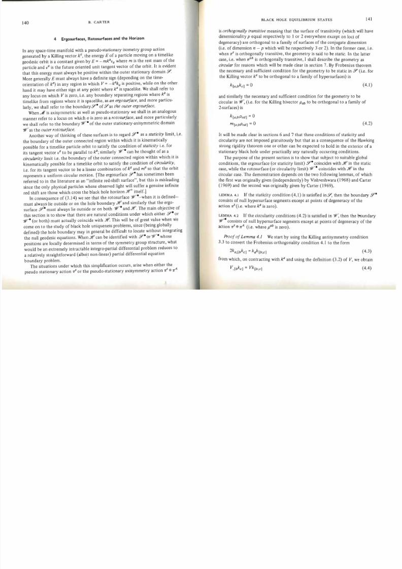
8/7/2019 b carter - equilibrium states of black holes
http://slidepdf.com/reader/full/b-carter-equilibrium-states-of-black-holes 43/48
4 Ergosurfaces, Rotosurfaces and the Horizon
In any space-time manifold with a pseudo-stationary isometry group action
generated by a Killing vector kG, the energy E of a particle moving on a timelike
geodesic orbit is a constant given by E = - m ~ v a where m is the rest mass of the
particle and va is the future oriented unit tangent vector of the orbit. It is evident
that this energy must always be positive within the outer stationary domain Y'.
More generally E must always have a definite sign (depending on the time
orientation of k a) in any region in which V = - ~ k a is positive, while on the other
hand it may have either sign at any point where kais spacelike. We shall refer to
any locus on which V is zero, i.e. any boundary separating regions where is
timelike from regions where it is spacelike, as an ergosurface, and more particu
larly, we shall refer to the boundary Y'. of Y' as the outer ergosurfacc.
When J l is axisymmetric as well as pseudo-stationary we shall in an analogous
manner refer to a locus on which a is zero as a rotosurface, and more particularly
we shall refer to the boundary if/. of the outer stationary-axisymmetric domain
11/ as the outer rotosurface.
Another way of thinking of these surfaces is to regard Y'. as a staticity limit, i.e.
the boundary of the outer connected region within which it is kinematically
possible for a timelike particle orbit to satisfy the condition of staticity i.e. forits tangent vector va to be parallel to similarly if/. can be thought of as a
circularity limit i.e. the boundary of the outer connected region within which it is
kinematically possible for a timelike orbit to satisfy the condition of circularity,
i.e. for its tangent vector to be a linear combination of ka
and rna so that the orbit
represents a uniform circular motion. [The ergosurface Y'. has sometimes been
referred to in the literature as an "infinite red-shift surface", but this is misleading
since the only physical particles whose observed light will suffer a genuine infinite
red shift are those which cross the black hole horizonyr itselL]
In consequence of (3.14) we see that the rotosurface if/·-when it is defined
must always-lie outside or on the hole boundary lI f and similarly that the ergo
surface Y'. must always lie outside or on both 11/. and lIf. The main objective of
this section is to show that there are natural conditions under which either Y'. or
11/. (or both) must actually coincide with Yf. This will be of great value when We
come on to the study of black hole uniqueness problems, since (being globally
defined) the hole boundary may in general be difficult to locate without integrating
the null geodesic equations. When l If can be identified with Y'. or ir· whose
positions are locally determined in terms of the symmetry group structure, what
would be an extremely intractable integro-partial differential problem reduces to
a relatively straightforward (albeit non-linear) partial differential equation
boundary problem.
The situations under which this simplification occurs, arise when either the
pseudo stationary action "If or the pseudo-stationary axisymmetry action "If ffi rr4
is orthogonally transitive meaning that the surface of transitivity (which will have
dimensionality p equal respectively to 1 or 2 everywhere except on loci of
degeneracy) are orthogonal to a family of surfaces of the conjugate dimension
(i.e. of dimension n - p which will be respectively 3 or 2). In the former case, i.e.
when rrs is orthogonally transitive, the geometry is said to be static. In the latter
case, i.e. when rrsA is orthogonally transitive, I shall describe the geometry as
circular for reasons which will be made clear in section 7. By Frobenius theorem
the necessary and sufficient condition for the geometry to be static in Y' (Le. for
the Killing vector ka
to be orthogonal to a family of hypersurfaces) is
k[a;bkc] = 0 ( 4.1)
and similarly the necessary and sufficient condition for the geometry to be
circular in 11/, (i.e. for the Killing bivector Pab to be orthogonal to a family of
2-surfaces) is
k[a;bPcd] = 0
m[a;bPcd] = a (4.2)
It will be made clear in sections 6 and 7 that these conditions of staticity and
circularity are not imposed gratuitously bu t that as a consequence of the Hawking
strong rigidity theorem one or other can be expected to hold in the exterior of astationary black hole under practically any naturally occurring conditions.
The purpose of the present section is to show that subject to suitable global
conditions, the ergosurface (or staticity limit) Y'. coincides with lI f in the static
case, while the rotosurface (or circularity limit) if/ . coincides with lI f in the
circular case. The demonstration depends on the two following lemmas, of wh.ich
the first was originally given (independently) by Vishveshwara (1968) and Carter
(1969) and the second was originally given by Carter ( 1969).
LEMMA 4.1 If the staticity condition (4.1) is satisfied inY', then the boundary Y'.
consists of null hypersurface segments except at points of degeneracy of the
action "If (i.e. where is zero).
LEMMA 4.2If
the circularity conditions (4.2)is
satisfied in if/, then the lroundaryif/. consists of null hypersurface segments except at points of degeneracy of the
action "If ffi rr4 (i.e. where pab is zero).
Proofo fLemma 4.1 We start by using the Killing antisymmetry condition
3.3 to convert the Frobenius orthogonality condition 4.1 to the form
2ka;[bkc] = kak[b;c] (4.3)
from which, on contracting with and using the definition (3.2) of V, we obtain
V,[bkc] = Vk[b;C] (4.4)
142143
B. CARTERBLACK HOLE EQUILIBRIUM STATES

8/7/2019 b carter - equilibrium states of black holes
http://slidepdf.com/reader/full/b-carter-equilibrium-states-of-black-holes 44/48
This tells us immediately that on the locus Y - on which V is zero, the gradient
V, b is parallel to JCl and hence null there, (except at points of degeneracy where
JCl is actually zero). In the non-degenerate case, i.e. when the gradient V,b is non
zero, so that V, b determines the direction of the normal to the hypersurface on
which V = 0, it follows immediately that this hypersurface is a null hypersurface
as required. In the degenerate case where V, b is zero on the locus V = 0 more care
is required since V might be zero not just on a hypersurface but over a domain of
finite measure. However by more detailed consideration of the situation (cf. Carter
(1969)) it can easily be verified that it will still be true that the actual boundary
Y- must be a null hypersurface.
Proof o f Lemma 4.2 By analogy with the previous case, we use the Killing
antisymmetry conditions (3.4) and (3.8) to convert the Frobenius orthogonality
conditions (4.2) to the form
ka;lbPcd] = -kak[b;cmd] + mak[b;ckdl } (4.5)ma;[bPcd] = mam[b;cmd] - kam[b;cmd]
from which we can directly obtain
(4.6)2Pae;[bPcd] = PaeP[cd;b]
Contracting this with the Killing bivector Pab we obtain
(4.7)a,[bPcd] =aPlcd;b]
This equation is analogous to (4.4), and tells us immediately that in the non
degenerate case, i.e. when the gradient a b is non-zero on the boundary ifI- where
a is zero, the normal toi f l - which is pa;allel to a,b lies in the plane of the Killing
bivector Pab' This is only possible (since the normal must also be orthogonal to
this bivector) if the normal is null, i.e. if ifI- is a null hypersurface. As before it is
still possible with rather more care (see Carter 1969) to deduce that the boundary
ifI- is a null hypersurface even in the degenerate case where a,b is zero, (except
on the lower dimensional surfaces of degeneracy of the group action, where the
Killing bivector Pab is itself zero). This completes the proof.
The two preceding lemmas may be used respectively in conjunction with thelemma of section 2, to prove the two following theorems, which are of central
importance in stationary black hole theory: (these results have been given in a
somewhat more general mathematical context by Carter 1972b).
THEOREM 4.1 (Static Ergosurface Theorem) Let Jt be a pseudo-stationary
asymptotically flat space-time manifold with asimply-connected domain of outer
communications ~ f } > . Then if the (chronological) causality axiom and the
staticity condition (4.1) are satisfied in ~ f } > it follows that ~ f } > = Y, where
Yis the outer stationary domain and hence that the outer ergosurfaceY
coincides with the hole boundary::lf.
THEOREM 4.2 (Rotosurface Theorem) Let Jt be a pseudo-stationary axisymmetric
asymptotically flat space-time manifold with asimply connected domain of outer
communications ~ f } > . Then if the causality axiom and the circularity condition
(4.2) are satisfied in ~ f } > it follows that ~ f } > =iflwhere if I is the outer
stationary-axisymmetry domain, and hence that the outer rotosurface ifIcoincides with the hole boundary JIf
Proof o f Theorem 4.1 We have already noted that Y must always be entir ely
contained within ~ f } > . Let be a connected component of the complement of,SPin ~ f } > . SinceYis connected (by definition) so also is the complement of
in ~ f } > . Hence by the condition that ~ f } > is simply connected, it follows (from
elementary homotopy theory) that the boundary of as restricted to ~ f } > , is connected.
Now (as we remarked at the end of section 2) it follows from the causality
axiom by the corollary to Lemma 2 that the action .,r can never be degenerate
(i.e. JCl can never be zero) in ~ f } > , and hence it follows from Lemma 4.1 that the
boundary £?2- of as restricted to ~ f } > , must consist entirely of one connected
null hypersurface. It follows that the outgoing normal (from of this hyper
surface must therefore be everywhere future directed or everywhere past directed;
in the former case no future directed timelike line in ~ f } > could ever enter
from Y, and in the latter case no future directed timelike line in ~ f } > could ever
enter Y from Neither alternative is compatible with the condition that lies
in ~ f } > , unless is empty. This establishes the required result.
Proof of Theorem 4.2 By analogy with the previous case we note that if Imust lie entirely within ~ f } > , and we choose £?2 to be a connected component
of the complement of if I in ~ f } > . As before we see that the boundary £?2- of
as restricted to ~ f } > , is connected.
We now use the causality axiom to establish that the action .,r Ell 0 is nowhere
degenerate (i.e. the Killing bivector Pab is nowhere zero) in ~ f } > except on the
rotation axis where mais zero. This follows from the fact that JCl must be parallel
to ma at any point of degeneracy, so that the trajectories of the action .,r would
be circles. Any such circular trajectory of .,r must lie outside ~ f } > if the
causality axiom holds, by the corollary to Lemma 2.We can now use Lemma 4.2 to deduce that the boundary of as restricted
to ~ . f } > must consist of a null hypersurface everywhere, except perhaps at points
on the rotation axis where ma is zero. We can go on to deduce that the outgoing
normal to this boundary must be everywhere future directed or everywhere past
directed as before, despite the possibility of degeneracy on the rotation axis, since
the rotation axis must be a timelike 2-surface everywhere (by local geometrical
considerations) and as such could never form the boundary of a null hypersurface.
Hence as in the previous case we deduce that must be empty as required. This
completes the proof.
144145
B. CARTERBLACK HOLE EQUILIBRIUM STATES

8/7/2019 b carter - equilibrium states of black holes
http://slidepdf.com/reader/full/b-carter-equilibrium-states-of-black-holes 45/48
.The mathematically important qualification that the domain of outer communica
tions should be simply connected does not restrict the practical application of
these theorems, since Stephen Hawking has given arguments (see his discussion in
the accompanying lecture course) which indicate that in any reasonably well
behaved gravitational collapse situation the domain of outer communications of
the resulting final equilibrium state should have the topology of the product of
the Euclidean line R(l) with a 3-space which has the form of a Euclidean R(3)
from which a number of three dimensional balls (solid spheres) have been removed,and which is therefore n2cessarily simply connected. Except in artificially con
trived situations one would expect further that the 3-space would have the form
of a Euclidean 3-space from which only one 3-dimensional ball has been removed ,
i.e. that it would have the topology S(2) x R( I) where S(2) is the 2-sphere, so that
the domain of outer communications as a whole would have the topology
S(2) x R(2). This latter stronger condition will be imposed in the theorems of
sections 10 to 13.We shall conclude this section by proving an important corollary to Theorem
4.2, which is as follows :
COROLLARY TO THEOREM 4.2 (Rigidity Theorem ) Under the conditions of
Theorem 4.2, it is possible to choose the normalization of the null tangent vector
la of in such a way that it has the form la=fC1+nH ma (4.8)
where the scalar nH is a constant over any connected component of +
Proof It is evident from (4.2) that la is a linear combination of fC1 and rna
on the horizon, and hence can be expressed in the form (4.8) where nH
is some
scalar which represents the local angular velocity of the horizon. The non trivial
part of the proof is the demonstration that nH is constant, i.e. that the rotation
which it determines is rigid, which is a consequence of the commutation condition
(3.8), which was not required for the proof of the basic Theorem 4.2. Since any
vector in the horizon including rna in particular, is orthogonal to la we find on
contracting (4.8) with rna that nHmust be given by
xn
H= -w (4 .9)
where Wand X are defined by (3.12) and (3.6). (On the rotation axis, where W
and X are both zero, nH must be defined by a limiting process). Using the
relations
X,a =2mbmb;D } W =2kb (4.10)
,a mb;a
(o f which the latter is a consequence of the commutation condition (3.8)) we find
by differentiation of (4.9) that the gradient of nH
is given by
x 2 n ~ =2[Wmb _ Xkb]mb;a (4 .11)
It follows, from the second of the Frobenius equations (4.2), that we must have
X2n1aPbcI = -40m(a;b:nc] ( 4 .12)
where 0 is defined by (3.11). Since we have already established that 0 is zero on
the horizon, this gives simply
njaPbC] =0 (4 .13)
This implies that the gradient of the coefficient nH determined by (4.9) lies in the
surface of transitivity of the group action 1fA at the horizon, which is impossible
(since nHis clearly a group invariant quantity) unless the gradient is actually zero
on the horizon, i.e.
nH=o (4.14), a
which is the required result. This completes the proof.
Having established that nHas defined by (4.8) is constant on the horizon , we
can use this constant in (4.8) to define a vector field la which will satisfy the
Killing equatio ns
la ;b = l(a;b I (4.15)
everywhere in JI . Our demonstration of the existence of this Killing vector field
la that is null on the horizon has been based on the assumption that either thestaticity condition or the axisymmetric circularity condition is satisfied . The
strong rigidity theorem of Hawking, to which we have already referred, establishes
the existence of this Killing vector field without assuming either staticity or ax i
symmetry, subject only to very weak and general assumptions. If the hole is
rotating, i.e. if la does not coincide with fC1 then Hawking has shown, as an
immediate corollary to his basic theorem, that there must exist an axisymmetry
action generated by a Killing vector field rna such that la has the form (4.8) . It
then follows from the generalized Papapetrou theorem which will be described in
section 7 that the circularity condition which was postulated in Theorem 4.2 must
necessarily hold. On the other hand if the hole is non-rotating, i.e. if the Killing
vector field la that is null on the horizon coinCides with the pseudo-stationary
Killing vector field fC1, it follows from the generalized Hawking-Lichnerowicz
theorem which will be described in section 6 that the staticity condition which
was postulated in Theorem 4.1 must necessarily hold (at least provided one is
prepared to accept the as yet no t rigorously proved supposition that the ergo
surface which coincides with the horizon in the non-rotating case is the same as
the outer ergosurface).
The net effect of the results of this section is to establish that .;!f+ must be a
Killing horizon (in the sense defined by Carter 1969) that is to say it is a null hyper
surface whose null tangent vector coincides (wh en suitably normalized) with the
representative of some (fixed) Killing vector field, this field being the la which has
just been constructed . This makes it possible to carry out a precise analysis of the
147146 B. CARTER BLAC K HOLE EQUILIBRIUM STATES
hence satisfies
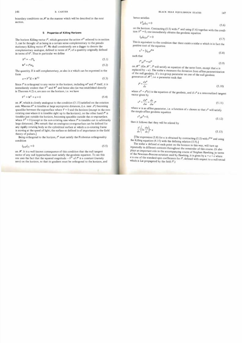
8/7/2019 b carter - equilibrium states of black holes
http://slidepdf.com/reader/full/b-carter-equilibrium-states-of-black-holes 46/48
5
boundary conditions on yt> in the manner which will be described in the next
section.
Properties of Killing Horizons
The horizon Killing vector la , which generates the action 7!"i' referred to in section
3, can be thought of as being in a certain sense complementary to the pseudo
stationary Killing vector k,'l. We shall consistently use a dagger to denote thecomplementary analogue, defined in terms of la, of a quantity originally defined
in terms of k,'l. Thus in particular we define
vt = -c-lala (5.1)
Wt =lama (5.2)
The quantity X is self complementary, as also is a which can be expressed in the
form
a =VtX + Wt2 (5 .3)
Since la is orthogonal to any vector in the horizon , including ma and la itself, it is
immediately evident thatvt
andWt
and hence also (as was established directlyin Theorem 4.2) a, are zero on the horizon, i.e. we have
Wtvt = =a =0 (5.4)
on yt>, which is closely analogous to the condition (3 .13) satisfied on the rotation
axis. Whereas k,'l is timelike at large asymptotic distances, (i.e . near .Y) becoming
spacelike bet ween the ergosurface where V = 0 and the horizon (except in the non
rotating case where it is timelike right up to the horizon), on the other hand la is
timelike just outside the horizon, becoming space like o utside the co-ergosurface,
where vt =0 (except in the n on-rotating case where la is timelike ou t to arbitrarily
large distances). [We remark that an analogous co-ergosurface can be defined for
any rigidly rotating body as the cylindrical surface at which a co-rotating frame
is moving at the speed of light; the surface so defined is of importance in the Goldtheory of pulsars.]
Being orthogonal to the horizon, la must satisfy the Frobenius orthogonality
condition
l(a;blc J = 0 (5.5)
on yt>. It is a well known consequence of this condition that the null tangent
vector of any null hypersurface must satisfy the geodesic equation . To see this
one uses the fact that the squared magnitude - vt of la is a constant (namely
zero) on the horizon, so that its gradient must be orthogonal to the horizon, and
V;(alb) = 0(5.6)
on the horizon. Contracting (5 .5) with lCand using (5.6) together with the condi
tion vt = 0, one immediately obtains the geodesic equatio n
l[alb );clc =0(5.7)
This is equivalent to the condition that there exists a scalar K which is in fact the
positive root of the equation
K2 = 11 lb;a2 a;b
(5.8)such that
la;blb = Kia (5 .9)
on yt>+. (On YIf -, la will satisfy an equation of the same form , except that K is
replaced by - K). The scalar Kmeasures the deviation from affine parametrization
of the null geodesic. If v is a group parameter on one of the null geodesic
generators of yt> +, i.e. a parameter such that
dxa
l a=_
dv (5 .10)
awhere x = xa(v) is the equation of the geodesic, and if va is a renormalized tangentvector given by
a dv av =-=-1 (5.11 )
dw dw
where w is an affine parameter , i.e. a function of v chosen so that va will satisfy the simple affine geodesic equation
va. vb:: 0,b ,(5 .12)
then it follows that they will be related by
(I n dW):: K
dv dv (5.13)
[The expression (5.8) for K is obtained by contracting (5 .5) with lb;a and using
the Killing equation (4.15) with the defining relation (5.9).]
The scalar K defined at each point on the horizon in this way, will turn up
repeatedly in different contexts throughout the remainder of this Course. (I t also
plays an important role in the accompanying course of Stephen Hawking; in terms
of the Newman-Penrose notation used by Hawking, it is given by K = € +Ewhere
€ is one of the standard spin coefficients for la , defined with respect to a null-tetradwhich is Ue propagated by the field la.) .
148149B. CARTER
This scalar was first discussed explicitly by Boyer in some work which was
BLACK HOLE EQUILIBRIUM STATES
hypersurfaces are Killing horizons on which vt is zero . [Both Boyer himself in his
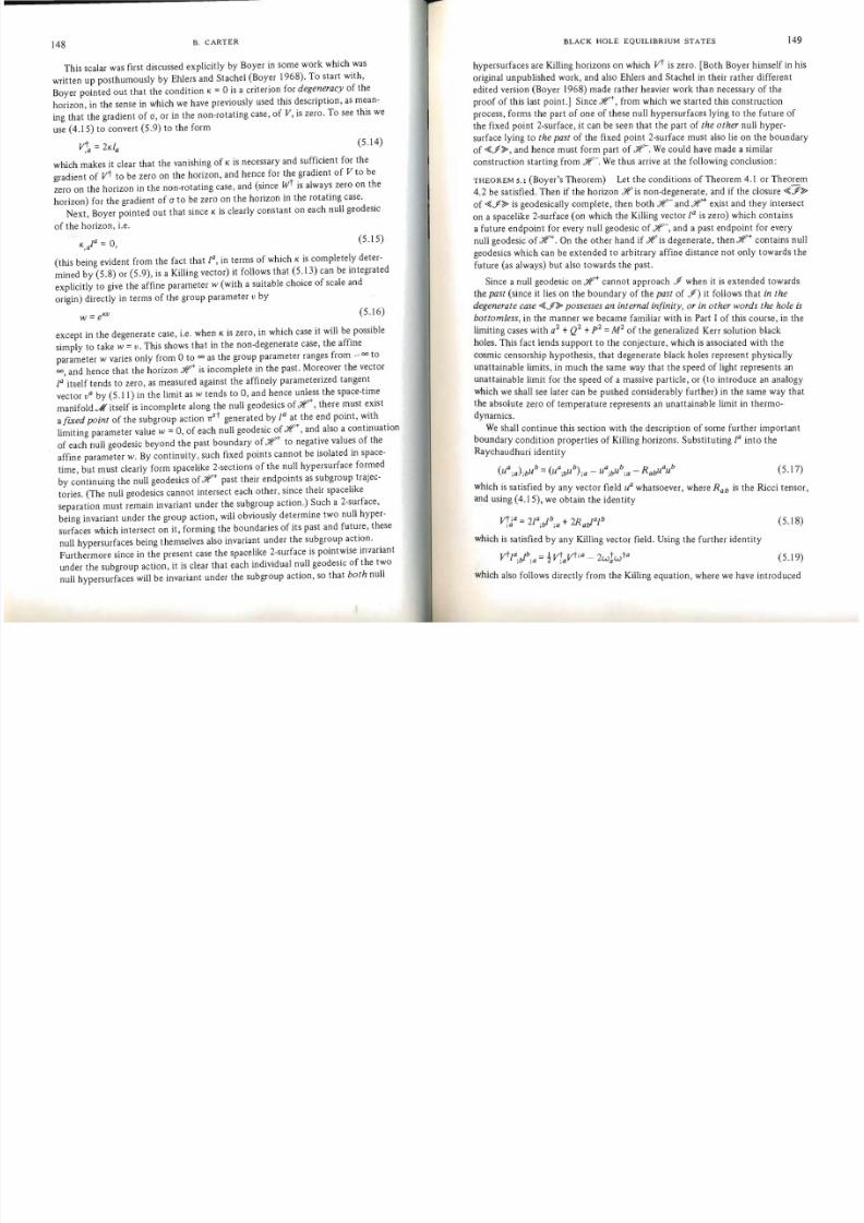
8/7/2019 b carter - equilibrium states of black holes
http://slidepdf.com/reader/full/b-carter-equilibrium-states-of-black-holes 47/48
written up posthumously by Ehlers and Stachel (Boyer 1968). To start with,
Boyer pointed out that the condition K= 0 is a criterion for degeneracy of the
horizon, in the sense in which we have previously used this description, as mean
ing that the gradient of a, or in the non -rotating case, of V, is zero. To see this we
use (4.IS) to convert (S.9) to the form
(S .14)vt,a = 2Kla
whichmakes it
clearthat the
vanishingof K is
necessary and sufficient forthe
gradient of vt to be zero on the horizon , and hence for the gradient of V to be
zero on the horizon in the non-rotating case, and (since Wt
is always zero on the
horizon) for the gradient of a to be zero on the horizon in the rotating case.
Next, Boyer pOinted out that since K is clearly constant on each null geodesic
of the horizon , i.e.
K,aLa = 0, (S.IS)
(this being evident from the fact that la, in terms of which K is completely deter
mined by (S.8) or (S.9), is a Killing vector) it follows that (S.13) can be integrated
explicitly to give the affine parameter w (with a suitable choice of scale and
origin) directly in terms of the group parameter v by
KV (S.16)
w =eexcept in the degenerate case, i.e. when K is zero, in which case it will be possible
simply to take w =v. This shows that in the non-degenerate case, the affine
parameter w varies only from 0 to 00 as the group parameter ranges from _00 to
00 , and hence that the horizon Yt'+ is incomplete in the past. Moreover the vector
La itself tends to zero , as measured against the affinely parameterized tangent
vector va by (S.II) in the limit as w tends to 0, and hence unless the space-time
manifold J( itself is incomplete along the null geodesics of f , there must exist
a fixed point of the subgroup action 1ft generated by la at the end point, with
limiting parameter value w = 0, of each null geodesic of JIt+, and also a continuation
of each null geodesic beyond the past boundary of yt+ to negative values of the
affine parameter w. By continuity, such fixed points cannot be isolated in space
time, but must clearly form spacelike 2-sections of the null hypersurface formedby continuing the null geodesics of ,;tt'+ past their endpoints as subgroup trajec
tories. (The null geodesics cannot intersect each other, since their spacelike
separation must remain invariant under the subgroup action.) Such a 2-surface,
being invariant under the group action, will obviously determine two null hyper
surfaces which intersect on it , forming the boundaries of its past and future, these
null hypersurfaces being themselves also invariant under the subgroup action.
Furthermore since in the present case the spacelike 2-surface is pointwise imariant
under the subgroup action, it is clear that each individual null geodesic of the two
null hypersurfaces will be invariant under the subgroup action, so that both null
original unpublished work, and also Ehlers and Stachel in their rather different
edited version (Boyer 1968) made rather heavier work than necessary of the
proof of this last point.] Since yr+, from which we started this construction
process, forms the part of one of these null hypersurfaces lying to the future of
the fixed point 2-surface, it can be seen that the part of the other null hyper
surface lying to the past of the fixed point 2-surface must also lie on the boundary
of ~ J P ~ , and hence must form part of f . We could have made a similar
construction starting from JIt-. We thus arrive at the following conclusion:
THEOREM 5.1 (Boyer's Theorem) Let the conditions of Theorem 4.1 or Theorem
4.2 be satisfied. Then if the horizon ,;tt'is non-degenerate, and if the closure ~ J P ~ of ~ J P ~ is geodesically complete, then both f and f exist and they intersect
on a space like 2-surface (on which the Killing vector la is zero) which contains
a future endpoint for every null geodesic of ,;tt'-, and a past endpoint for every
null geodesic of Yf+. On the other hand if ,;tt' is degenerate, then yt'+ contains null
geodesics which can be extended to arbitrary affine distance not only towards the
future (as always) but also towards the past.
Since a null geodesic on Yt'+ cannot approach JP when it is extended towards
the past (since it lies on the boundary of the past of JP ) it follows that in the
degenerate case ~ J P ~ possesses an internal infini ty, or in other words the hole is
bottomless, in the manner we became familiar with in Part I of this course, in the
limiting cases with a2+Q2 + p2 = M2 of the generalized Kerr solution black
holes. This fact lends support to the conjecture, which is associated with the
cosmic censorship hypothesis, that degenerate black holes represent physically
unattainable limits, in much the same way that the speed of light represents an
unattainable limit for the speed of a massive particle, or (t o introduce an analogy
which we shall see later can be pushed considerably further) in the same way that
the absolute zero of temperature represents an unattainable limit in thermo
dynamics.
We shall continue this section with the description of some further important
boundary condition properties of Killing horizons. Substituting la into the
Raychaudhuri identity
( a) b _ (a b) a bR a b (S.17)U ;a ;bU - U ;bU ;a - U ;bU ;a - abU U
which is satisfied by any vector field ua whatsoever, where Rab is the Ricci tensor,
and using (4.IS), we obtain the identity
vtJa= 2Ia;blb;a+ 2 R a ~ a l b (S.18)
which is satisfied by any Killing vector field. Using the further identity
Vtla;blb;a = VTavt ;a - 2wjw ta (S .19)
which also follows directly from the Killing equation , where we have introduced
151150 B. CARTER
the rotation vector w ta of the field given by
BLACK HOLE EQUILIBRIUM STATES

8/7/2019 b carter - equilibrium states of black holes
http://slidepdf.com/reader/full/b-carter-equilibrium-states-of-black-holes 48/48
w! =1Eabcdlbld;C (5.20)
(where Eabcd is the alternating tensor) (5.19) can be expressed as
,,+ Vt;a 4 t tavt;a = v;a - wa W + 2R alb
abl (5.21 ); a vt
Evaluating the various terms on the horizon , we deduce directly from (4 .15) and
(5.9) that the Laplacian of vt takes the value
vt ;a.a=4K 2 (5.22)
on Y't, and hence from (5.8) and (5.18) that
Rablalb = 0 (5.23)
on Y't. Since, by (5.5) the rotation vector w! is zero on Yf' it is clear in the non
degenerate case, and can be verified to be true even in the degenerate limit case,
that the ratio w!w ta / Vt tends to zero on Y't; it therefore follows that
Viavt ;a~ - 7 K 2 (5,24)
in the limit on Yf'. This last equation gives rise to another interpretation ofK.
Theacceleration aa of an observer rigidly co-rotating with the hole, i.e. following one
of the trajectories of the field la , is given by
vtaa =la.blb (5.25)
Introducing the convention (which will be employed frequently in the following
sections) of using a bar to denote quantities associated with orbits which have
been renormalized by multiplication by the time dilatation factor of the orbit
(which in this case is Vt 1/2), we define
(;a = vt 1/2tf (5.26)
In terms of this renormalized acceleration vector, we see that (5 .24) has the form
aaaa -7 K2 (5.27)
on Yf', i.e. K represents the limiting magnitude of the renormalized acceleration of
a co-rotating observer.
Since ordinary matter will always give positive contributions to Rablalb
, the
equation (5.23) implies that the immediate neighbourhood of the hole boundary
must always be empty, except possibly for the presence of an electromagnetic
field, which can be contrived so as to give zero contribution to the term Rablalb.
The restrictions required to satisfy this requirement are rather stringent however,
and place well defined boundary conditions on the field. Introducing the Maxwell
energy tensor rzl, which will be proportional to the Ricci tensor under these
conditions, by
rzl = 4rrI [FacFg - !FcdFcdi'b] (5.28)
where Fab is the electromagnetic field tensor, we obtain
1TFablal
b= 8rr [E1fft a
+meta] (5.29)
where we have introduced the co-rotating electric and magnetic field vectors £1and jj! defined by
ffta = FabIb (5.30)
jj t = -k E r:edlba <- abcd r (5.31)
Since they are both orthogonal to la , neither can be timelike within the closure of
f ~ , so that (5.29) is a sum of non-negative terms. Thus Rablalb and T pablalb
can only be zero on Yf' if £! and Bl are both null on and hence (by the ortho
gonality) parallel to la on Yf'. In other words the electromagnetic field must
satisfy the boundary conditions
£ ( ~ / b l =0 (5.32)- tB/albJ = 0 (5.33)
on Yf'.
6 Stationarity, Staticity, and the Hawking-Lichnerowicz Theorem
The terms stationary and static are used widely in different physical contexts.
Generally speaking a system is said to be stationary if it is invariant under a
continuous transformation group which maps earlier events into later ones. In
General Relativity this condition can be more precisely defined in terms of the
requirement that space-time be invariant under the action of a continuous one
parameter isometry group generated by a Killing vector field which is either timelike everywhere (in which case the space-time is said to be stationary in the strict
sense) or else timelike at least somewhere, e.g. in sufficiently distant asymptotic
ally flat region, (in which case I shall refer to the space-time as pseudo-stationary).
It is not quite so easy to give a definition of what is meant by the statement that
a general physical system is static, without referring to the specific context, but
broadly speaking a system is said to be static if it is not only stationary in the
strict sense, bu t also such that there is no motion (i .e. no material flow or current)
relative to the stationary reference system. How this is to be interpreted will of
COurse depend on which kinds of flow or current are relevant. For example a river


![Thermodynamics in modified gravity - University of … · [Bardeen, Carter and Hawking, Commun. Math. Phys. 31, 161 (1973)] ... Thermodynamics in modified gravity-non-equilibrium](https://static.documents.pub/doc/80x56/5b93076909d3f209728d071c/thermodynamics-in-modified-gravity-university-of-bardeen-carter-and-hawking.jpg)


