B. Introduction to the Final Report

Justin R. Fulkerson, E. Jamie Trammell, Matthew L. Carlson, and Monica

McTeague

Alaska Center for Conservation Science, University of Alaska Anchorage, 3211 Providence Dr.,

Anchorage, Alaska 99508.

Summary

Section B. Introduction to the Final Report provides an overview of the REA process, general

methodological approaches, study area, Conservation Elements, Change Agents, Management

Questions, and limitations.

Page Intentionally Left Blank

B-iii

Section B. Introduction

Contents

1. What is a Rapid Ecoregional Assessment? ..........................................................................................B-1

2. Approach and Process ..........................................................................................................................B-2

2.1. Change Agents (CAs) ................................................................................................................B-2

2.2. Conservation Elements (CEs) ...................................................................................................B-2

2.3. Management Questions .............................................................................................................B-5

2.4. Conceptual Models ....................................................................................................................B-8

2.5. Attributes and Indicators ............................................................................................................B-9

2.6. CE × CA Analyses ...................................................................................................................B-10

2.7. Process Models .......................................................................................................................B-12

2.8. Land Owners and Stakeholders ..............................................................................................B-13

2.9. Project Team ............................................................................................................................B-14

3. Description of Rapid Ecoregional Study Area .....................................................................................B-16

3.1. Brooks Range ..........................................................................................................................B-17

3.2. Davidson Mountains ................................................................................................................B-17

3.3. Kobuk Ridges and Valleys .......................................................................................................B-18

3.4. North Ogilvie Mountains ..........................................................................................................B-18

3.5. Ray Mountains .........................................................................................................................B-19

3.6. Yukon – Old Crow Basin ..........................................................................................................B-19

3.7. Yukon-Tanana Uplands ...........................................................................................................B-20

3.8. Assessment Boundary and Scale ............................................................................................B-20

3.9. Ecoregional Conceptual Model ................................................................................................B-21

4. Assessing Current and Future Conditions ..........................................................................................B-23

5. Scope, Intent, and Limitations .............................................................................................................B-24

6. Literature Cited ....................................................................................................................................B-25

B-iv

Section B. Introduction

Tables

Table B-1. Change Agents and Conservation Elements selected for the Central Yukon REA. .............. B-4

Table B-2. MQs selected by the AMT for analysis as part of the Central Yukon REA............................. B-6

Table B-3. Total area and percent of study area by land management status. ..................................... B-14

Figures

Figure B-1. Conventions for conceptual models. ..................................................................................... B-8

Figure B-2. Explanation and example of attributes and indicators tables. ............................................. B-10

Figure B-3. Example conceptual model for chum salmon. .................................................................... B-11

Figure B-4. Conventions for Process Models. ....................................................................................... B-12

Figure B-5. Land management status in the Central Yukon study area in 2015. .................................. B-13

Figure B-6. Ecoregions included in the Central Yukon study area. ....................................................... B-16

Figure B-7. Chandalar Shelf of the Brooks Range. ............................................................................... B-17

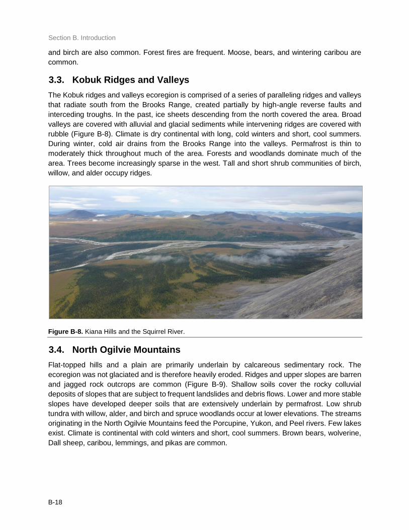
Figure B-8. Kiana Hills and the Squirrel River. ...................................................................................... B-18

Figure B-9. Calcareous rock outcrops and ridges in the North Ogilvie Mountains. ............................... B-19

Figure B-10. Floodplain and extensive flats along the Porcupine River. ............................................... B-20

Figure B-11. Eagle Summit in the White Mountains. ............................................................................. B-20

Figure B-12. Ecoregional Conceptual Model for the Central Yukon study area. ................................... B-22

Figure B-13. Example process of assessing status of a Conservation Element (CE). Landscape condition

(A) is extracted to the distribution of a CE (B) to generate the CE status (C). Warmer colors in the CE status

represent areas of lower expected ecological condition. ........................................................................ B-23

B-1

Section B. Introduction

1. What is a Rapid Ecoregional Assessment?

The Bureau of Land Management (BLM) recently developed a landscape approach to enhance

management of public lands (BLM 2014). As part of this landscape approach, the BLM and

collaborators are conducting Rapid Ecoregional Assessments (REAs) in the western United

States, including Alaska. To address current problems and future projections at the landscape

level, the REAs are designed to transcend management boundaries and synthesize existing data

at the ecoregion level. A synthesis and analysis of available data benefits the BLM, other federal

and state agencies, and public stakeholders in the development of shared resources (Bryce et al.

2012).

REAs evaluate questions of regional importance identified by land managers, and assess the

status of regionally significant ecological resources, as well as Change Agents that are perceived

to affect the condition of those ecological resources. The resulting synthesis of regional

information is intended to assist management and environmental planning efforts at multiple

scales. REAs have two primary purposes:

To provide landscape-level information needed in developing habitat conservation

strategies for regionally significant native plants, wildlife, and fish and other aquatic

species.

To inform subsequent land use planning, trade-off evaluation, environmental analysis, and

decision-making for other public land uses and values, including development, recreation,

and conservation.

Once completed, this information is intended to provide land managers with an understanding of

current resource status and the potential for future change in resource status in the near-term

future (year 2025) and long-term future (year 2060).

Four REAs have recently been completed in Alaska. These include the Seward Peninsula

(Harkness et al. 2012), Yukon Lowlands – Kuskokwim Mountains – Lime Hills (Trammell et al.

2014), the North Slope (Trammell et al. 2015), and the Central Yukon (current document).

B-2

Section B. Introduction

2. Approach and Process

To address the regionally important questions, significant ecological resources, and patterns of

environmental change, REAs focus on three primary elements:

Change Agents (CAs) are features or phenomena that have the potential to affect the

size, condition, and landscape context of ecological systems and components.

Conservation Elements (CEs) are biotic constituents or abiotic factors of regional

importance in major ecosystems and habitats that can serve as surrogates for ecological

condition across the ecoregion.

Management Questions (MQs) are regionally specific questions developed by land

managers that identify important management issues.

MQs focus the REAs on pertinent management and planning concerns for the region. MQs are

used to select CEs and CAs by identifying critical resources and management concerns for the

study area. CEs are also identified by an Ecoregional Conceptual Model (see Section B.3.9.

Ecoregional Conceptual Model). Although a basic list of CAs is provided by the BLM, MQs can

also identify regionally-specific CAs to be considered in the analysis. An important strength of this

approach is the integration of current management concerns and current scientific understanding

into a comprehensive and forward-looking regional assessment.

The core REA analysis refers to the status and distribution of CEs and CAs and the intersection

of the two. The core REA analysis addresses the following five questions:

1. Where are Conservation Elements currently?

2. Where are Conservation Elements predicted to be in the future?

3. Where are Change Agents currently?

4. How might Change Agents be distributed in the future?

5. What is the overlap between Conservation Elements and Change Agents now and in the

future?

2.1. Change Agents (CAs)

CAs are those features or phenomena that have the potential to affect the size, condition, and

landscape context of CEs. CAs include broad factors that have region-wide impacts such as

wildfire, invasive species, and climate change, as well as localized impacts such as development,

infrastructure, and extractive energy development. CAs can affect CEs at the point of occurrence

as well as through indirect effects. CAs are also expected to interact with other CAs to have

multiplicative or secondary effects. Although they are listed separately, most anthropogenic CAs

generally occur in concert with one another. Mining and energy development, for example, require

other CAs like transportation and transmission infrastructure.

2.2. Conservation Elements (CEs)

Conservation Elements (CEs) are defined as biotic constituents (e.g., vegetation classes and

wildlife species, or species assemblages), abiotic factors (e.g., soils) of regional importance in

B-3

Section B. Introduction

major ecosystems and habitats across the ecoregion, or high biodiversity priority sites (e.g.,

designated Important Bird Areas). CEs are meant to represent key resources that can serve as

surrogates for ecological condition across the ecoregion.

The selected CEs are limited to a suite of specific ecosystem constituents that, if conserved,

represent key ecological resources and thus serve as a proxy for ecological condition. CEs are

defined through the “Coarse-filter / Fine-filter” approach, suggested by BLM guidelines; an

approach used extensively for regional and local landscape assessments (Jenkins 1976, North

Slopes 1987). This approach focuses on ecosystem representation as “Coarse-filter’s” with a

limited subset of focal species and species assemblages as “Fine-filter s”. The Coarse-filter / Fine-

filter approach is closely integrated with ecoregional and CE-specific modeling exercises (Bryce

et al. 2012).

Coarse-Filter Conservation Elements

Terrestrial and Aquatic Coarse-filter CEs include regionally significant terrestrial vegetation

classes and aquatic ecosystems within the study area. They are intended to represent the habitat

requirements of most characteristic native species, ecological functions, and ecosystem services.

Fine-Filter Conservation Elements

Fine-filter CEs represent species that are critical to the assessment of the ecological condition of

the Central Yukon study area for which habitat is not adequately represented by the Coarse-filter

CEs. Fine-filter CEs selected for the REA are regionally significant mammal, bird, and fish

species. A list of CAs and Coarse-filter and Fine-filter CEs is given in Table B-1.

B-4

Section B. Introduction

Table B-1. Change Agents and Conservation Elements selected for the Central Yukon REA.

Change Agents (CAs) Conservation Elements (CEs)

Coarse-Filter CEs Fine-Filter CEs

Climate Terrestrial Coarse-Filter Terrestrial Fine-Filter

Precipitation Alpine and Arctic Tussock Tundra

beaver (Castor canadensis)

Temperature Alpine Dwarf Shrub Tundra caribou (Rangifer tarandus)

Thaw Date Floodplain Forest and Shrub

golden eagle (Aquilia chrysaetos)

Fire Lowland Woody Wetland Swainson’s thrush (Catharus ustulatus)

Return Interval Upland Low Shrub Tundra Dall sheep (Ovis dalli)

Vegetation Response Upland Mesic Spruce Forest

snowshoe hare (Lepus americanus)

Permafrost Upland Mesic Spruce-Hardwood Forest

trumpeter swan (Cygnus buccinator)

Ground Temperature Aquatic Coarse-Filter Aquatic Fine-Filter

Active Layer Thickness Rivers and Large Streams chinook salmon (Oncorhynchus tshawytscha)

Invasive Species Small Streams (including Headwater streams)

chum salmon (Oncorhynchus keta)

Insect and Disease Large Connected Freshwater Lakes

Dolly Varden (Salvelinus malma)

Anthropogenic Uses Small Connected Freshwater Lakes

humpback whitefish (Coregonus pidschian)

Subsistence northern pike (Esox lucius)

Natural Resource Extraction sheefish /inconnu (Stenodus leucichthys)

Transportation and Communication Infrastructure

Recreation

Energy Development

B-5

Section B. Introduction

2.3. Management Questions

Management Questions (MQs) provide regional managers the opportunity to highlight specific

concerns relevant to the larger ecoregions, and provide a tangible way in which these REA efforts

can be translated into management plans and actions. The University of Alaska (UA) team

received an initial list of Management Questions from the BLM Central Yukon Field Office, who

spent substantial time and effort identifying regionally important resource questions.

Through our conversations with the BLM, the UA Team parsed out original multi-part questions

into distinct questions. Additionally, all of the original management questions from BLM had

overarching questions of “How reliable are these predictions? Are there other data/models which

provide information that is different than the output presented?”. These questions will be

addressed as a standard component to all analyses throughout the REA. Overall this process

produced a list of 78 potential MQs. The original list of MQs can be reviewed in CYR Memorandum

I (AKNHP et al. 2014).

Given the rapid nature of the REA, the BLM locally suggested we limit the number of MQs to

around 20 (with a maximum of 30). Based on the success of the North Slope REA MQ selection

process using the Delphi survey method (Hess and King 2002; Scolozzi et al. 2012; O’Neill et al.

2008) to prioritize and focus our MQs, the UA team employed the same approach for the Central

Yukon REA. The UA team asked AMT members to rank which 20 questions where their top

questions, which 20 additional questions where next priority (mid), and which questions were of

lowest priority to them (remove).

Each AMT member was asked to consider the following guidance from the BLM National

Operations Center (NOC) on how to craft an appropriate Management Question:

• Is the MQ about large-scale, region-wide issues?

• Can the MQ be answered by available geospatial information, remote

sensing, or acceptable surrogates at the landscape scale?

• If the MQ cannot be addressed spatially, would a literature review be an

appropriate use of the REA?

• If it is an inventory question, can it be addressed within the timeframe of

the REA?

• Does the MQ inform a specific practical management decision or resource

allocation to be made (i.e., Which areas due to resource vulnerability

require protection as ACEC's? Which areas should be avoided for

authorization of new roads or utility corridors?)

• Does the MQ identify the potential subsequent decision process and or

action associated with the answer to the question?

• Has the MQ been answered in another recently competed ecoregional

assessment and is there additional information that warrants reexamining

this issue?

Ten responses were received from the first ranking by the AMT, 18 MQs surfaced as being the

top or mid priority MQs by the majority of the voting members of the AMT Responses were

B-6

Section B. Introduction

presented to the AMT and Technical Team members during the first AMT meeting on September

5, 2014. Additional MQs were provided by the AMT and an additional round of ranking was done

to ensure the first ranking was agreed upon by the majority of the AMT.

The second round of MQ surveys resulted in seven responses. The results were tallied based on

ranks for each question then reordered based on those tallies. Questions that were consistently

ranked as either Top 20 or Mid 20 by over half of the voting AMT members were selected as our

final list of MQs (Table B-2). In addition to the to 20 MQs we also identified 12 alternative MQs

with almost half of the AMT agreeing on these questions being either top 20 or mid 20 MQs.

These questions were considered as replacement MQs if any of the final MQs cannot be

adequately addressed by the UA team, pending AMT approval. Alternative MQs can be reviewed

in CYR Memorandum I (AKNHP et al. 2014).

Table B-2. MQs selected by the AMT for analysis as part of the Central Yukon REA.

Abiotic Change Agents (Section C)

A1 How is climate change likely to alter the fire regime in the dominant vegetation classes and riparian zones?

B1 How is climate change likely to alter permafrost distribution, active layer depth, precipitation regime, and evapotranspiration in this region?

B2 What are the expected associated changes to dominant vegetation communities and CE habitat in relation to altered permafrost distribution, active layer depth, precipitation regime, and evapotranspiration?

C1 How will changes in precipitation, evapotranspiration, and active layer depth alter surface water availability and therefore ecosystem function (dominant vegetation classes)?

E1 How is climate change affecting the timing of snow melt and snow onset, spring breakup and green-up, and growing season length?

F3 How are major vegetation successional pathways likely to change in response to climate change, with special emphasis on increased shrub cover and treeline changes?

Anthropogenic Change Agents (Section E)

Q1 Which subsistence species (aquatic and terrestrial) are being harvested by whom and where is harvest taking place?

U1 Compare the footprint of all types of landscape and landscape disturbances (anthropogenic and natural changed) over the last 20 and 50 years.

U3 How and where is the anthropogenic footprint most likely to expand 20 and 50 years into the future?

Terrestrial Coarse-Filter Conservation Elements (Section G)

AH1

What rare, but important habitat types that are too fine to map at the REA scale and are associated with coarse- (or fine-) filter CEs that could help identify areas where more detailed mapping or surveys are warranted before making land use allocations (such as steppe bluff association with dry aspect forest)?

G1 Where are refugia for unique vegetation communities (e.g. hot springs, bluffs, sand dunes) and what are the wildlife species associated with them?

B-7

Section B. Introduction

G2 Which unique vegetation communities (and specifically, which rare plant species) are most vulnerable to significant alteration due to climate change?

Terrestrial Fine-Filter Conservation Elements (Section H)

AE1 Where is primary waterfowl (black scoter or trumpeter swan) habitat located?

L1 What are caribou seasonal distribution and movement patterns?

N3 How might sheep distribution shift in relation to climate change?

T1 The introduction of free-ranging reindeer herds to this region has been proposed. What areas would be most likely to biologically support a reindeer herd?

X1 What have the past cumulative impacts of road construction and mineral extraction been on terrestrial CE habitat and population dynamics?

X2

How might future road construction and mineral extraction infrastructure (e.g. both temporary and permanent roads [Umiat, Ambler, Stevens Village], pads, pipeline, both permanent and temporary) affect species habitat, distribution, movements and population dynamics (especially caribou, moose, sheep)?

Aquatic Conservation Elements (Sections I and J)

W2 How might future road construction and mineral extraction infrastructure (e.g. both temporary and permanent roads, pads, pipeline) affect fish habitat, fish distribution, and fish movements (especially chinook, chum, sheefish)?

V1 How does human activity (e.g. mineral extraction, gravel extraction) alter stream ecology and watershed health (i.e. water quantity, water quality, outflow/stream connectivity, fish habitat, and riparian habitat)?

B-8

Section B. Introduction

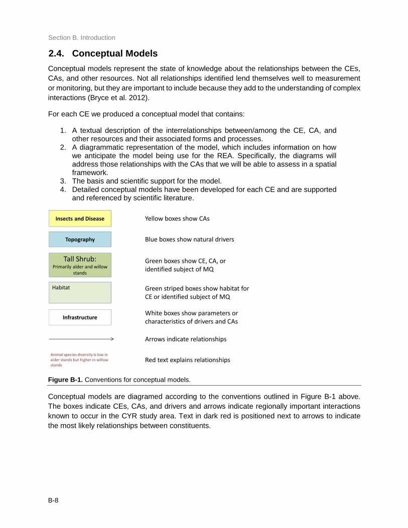
2.4. Conceptual Models

Conceptual models represent the state of knowledge about the relationships between the CEs,

CAs, and other resources. Not all relationships identified lend themselves well to measurement

or monitoring, but they are important to include because they add to the understanding of complex

interactions (Bryce et al. 2012).

For each CE we produced a conceptual model that contains:

1. A textual description of the interrelationships between/among the CE, CA, and other resources and their associated forms and processes.

2. A diagrammatic representation of the model, which includes information on how we anticipate the model being use for the REA. Specifically, the diagrams will address those relationships with the CAs that we will be able to assess in a spatial framework.

3. The basis and scientific support for the model. 4. Detailed conceptual models have been developed for each CE and are supported

and referenced by scientific literature.

Figure B-1. Conventions for conceptual models.

Conceptual models are diagramed according to the conventions outlined in Figure B-1 above.

The boxes indicate CEs, CAs, and drivers and arrows indicate regionally important interactions

known to occur in the CYR study area. Text in dark red is positioned next to arrows to indicate

the most likely relationships between constituents.

B-9

Section B. Introduction

2.5. Attributes and Indicators

Ecological attributes are defined as traits or factors necessary for maintaining a fully functioning

population, assemblage, community or ecosystem. On a species level, they are traits that are

necessary for species survival and long-term viability. Indicators are defined as measureable

aspects of ecological attributes. For REAs, we consider attributes and indicators as key elements

that allow us to better address specific management questions, help parameterize models, and

help explain the expected range of variability in our results as they relate to status and condition.

Attributes and indicators are a critical component of the core analysis as they help to define the

relationships between conservation elements (CEs) and change agents (CAs), and, where

possible, thresholds associated with these relationships.

For each Fine-filter CE, we identified a number of attributes derived from the conceptual model,

and assigned indicators based on available spatial data layers. Thresholds were set to categorize

all data into standard reporting categories (i.e., indicator ratings). For some CEs, numerical

measurements delineating thresholds were available from the literature. However, for many

attributes/indicators, categories were generalized based on the best available information, and

include (but are not limited to):

Poor – Fair – Good – Very Good – Unknown – None/NA

Low/none – Moderate – High – Very High – Unknown

Present – Absent – Unknown

Categorization of attributes/indicators has been adopted as a required element for all REAs.

Categorization allows data from a variety of sources to be organized similarly, whether the original

data were collected in categories or were collected as numerical measurements. It also allows

communication of information generated by complex REA analyses in an elegantly simple but

meaningful manner, and helps to provide consistency in assessing and reporting across the

variety of BLM resources, landscapes, and ecoregions.

We did not include attributes and indicators for Coarse-filter CEs. Alternatively, Coarse-filter CEs

status will be assessed using Landscape Condition Models and Cumulative Climate Impacts.

Here we provide an example (Figure B-2) of an attribute and indicator table for trumpeter swan

(Cygnus buccinator). This information is provided in summary table format for all Fine-filter CEs,

and is included with the individual CE conceptual model write-ups.

B-10

Section B. Introduction

Figure B-2. Explanation and example of attributes and indicators tables.

2.6. CE × CA Analyses

The purpose of the CE specific assessment is to evaluate the current status of each CE at the

ecoregional scale and to investigate how its status may change in the future as a result of future

development and climate change. The conceptual model for each CE helps guide the selection

of key ecological attributes and indicators that will assist us in assessing current and future status.

Ecological attributes and associated indicators, at the Fine-filter level, provide measures of the

acceptable range of variation for each ecological attribute to further assist with assessment of

status and trends.

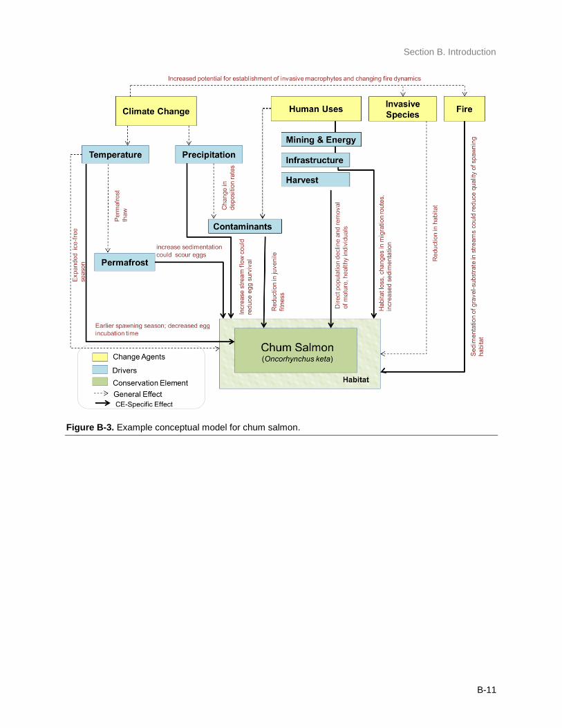
In each of the Fine-filter CE conceptual models, we have presented in bold lines those

relationships that we intend to analyze spatially based on available datasets (measureable

effects) as described in the attributes and indicators tables (Figure B-3). Although these analyses

will differ on a CE by CE basis, this process generally involves overlaying the distribution model

for each CE with the measureable CA indicator (e.g., fire, may affect sedimentation of gravel-

substrate in streams that could reduce the quality of spawning habitat of chum salmon).

B-11

Section B. Introduction

Figure B-3. Example conceptual model for chum salmon.

B-12

Section B. Introduction

2.7. Process Models

While conceptual models help inform the ecological relationships between ecosystem

components, drivers, and processes, process models illustrate computational relationships or

logical decisions within the context of a spatial or mathematical model to produce an output.

Process models diagram data sources, geoprocessing procedures, and workflows, providing

analytical transparency and allowing for repeatability of processes in the future (Bryce et al. 2012).

Process models have been developed to represent the analysis of each CA and MQ, and they

helped provide guidance for data discovery.

Process models are diagrammed according to the conventions in Figure B-4 below (Bryce et al.

2012). Each process model will contain the following:

1. A diagram illustrating data and methods. These are key elements (datasets

representing key attributes of CEs, CAs, and MQs) and procedures in the

computational process, the relationship among them, and the flow of information

and analyses.

2. Descriptive text explaining the diagram. Methods for developing process models

for all MQs are similar: source datasets are computationally or spatially related to

produce outputs that are further related to produce final products.

Figure B-4. Conventions for Process Models.

B-13

Section B. Introduction

2.8. Land Owners and Stakeholders

Figure B-5. Land management status in the Central Yukon study area in 2015.

Community meetings were an important part of this REA to ensure broader regional stakeholders

were included and informed about the effort. The UA team and BLM State and Field offices

coordinated informational meetings with the Fairbanks North Star Borough Planning Commission

as part of a series of three community meetings: the 1st meeting was held on 17 March 2015, the

2nd meeting was held 27 October 2015, and the 3rd meeting will be held after completion of the

project, tentatively scheduled for June 2016. The Planning Commission was chosen for our

community meetings, as Fairbanks holds the largest population of the region and has the largest

impact of individuals that can attend. An additional community meeting may be presenting final

results to a Resource Advisory Council meeting held 3–4 times a year across the state and is

attended by stakeholders from various interest groups such as tourism, energy, Alaska Native

organizations, environmental interest groups, and the public. During these meetings the UA team

informed the planning commission about the REA process, its expected outcomes, and gathered

input on CEs, CAs, and MQs.

A larger stakeholder group was also informed on the status of the assessment through a series

of four newsletters (spring 2015, summer 2015, fall 2015, and anticipated delivery summer 2016).

B-14

Section B. Introduction

Each newsletter was delivered by hard copy via the postal service and through e-mail, reaching

a group of almost 270 interested parties ranging from local business owners to state government

officials.

Additional stakeholder engagement came from the representatives of various state and federal

agencies that manage land parcels within the Central Yukon study area (Figure B-5) that served

on the Assessment Management Team (AMT) and Technical Team (Tech Team). The AMT and

Tech Team provided guidance and direction to the objectives of the assessment through regular

project communication and meetings (interim project memos and presentations can be accessed

online1). A full list of AMT and Technical Team members is included after the cover page. The

U.S. Fish and Wildlife Service, State of Alaska, National Park Service, Native groups, and Bureau

of Land Management are the primary land management agencies by area in the Central Yukon

study area (Table B-3).

Table B-3. Total area and percent of study area by land management status.

Land Ownership Area (km2) Percent of Total Study Area

Fish and Wildlife Service 103,004 26%

State Patent or TA 93,758 24%

National Park Service 66,959 17%

Native Patent or IC 49,510 13%

Bureau of Land Management 48,318 12%

State Selected 20,108 5%

Native Selected 7,223 2%

Water 3,665 0.9%

Department of Defense 3,034 0.8%

Private 238 0.06%

We used the most recent land ownership status data provided by the BLM at the start of this REA

analysis in 2014. By the completion of this project, land status changed in the CYR study area

where the State of Alaska relinquished approximately 700,000 acres of state-selected lands in

the upper Black River area. We recognize land status is constantly ever-changing and readers

should be aware of the limitations of all data used in our analyses.

2.9. Project Team

The Alaska Center for Conservation Science (ACCS) served as the lead for this REA, with close

collaboration from the Scenarios Network for Alaska and Arctic Planning (SNAP), and Institute of

Social and Economic Research (ISER). ACCS was formally known as the Alaska Natural Heritage

Program (AKNHP), but changed structure within the University of Alaska during the CYR

assessment. Throughout this document this team is collectively referred to as the University of

Alaska (UA) Team. The UA Team as a whole was responsible for assessing the current and

potential future status of CEs at the ecoregional scale and their relationships to CAs, as well as

1 See http://accs.uaa.alaska.edu/rapid-ecoregional-assessments/central-yukon-rea-documents

B-15

Section B. Introduction

addressing the Management Questions (MQs), identifying data gaps, and delivering data to the

BLM. Project leads are identified for the various sections reflecting the multi-disciplinal expertise

and knowledge used in assessing this region.

B-16

Section B. Introduction

3. Description of Rapid Ecoregional Study Area

The assessment area, referred to in this REA as the Central Yukon (CYR) study area, includes a

core of seven ecoregions selected by BLM: Brooks Range (south of the ridge crest), Davidson

Mountains, Kobuk Ridges and Valleys, North Ogilvie Mountains, Ray Mountains, Yukon – Old

Crow Basin, and Yukon-Tanana Uplands (Figure B-6). Ecoregions in this assessment were

defined by Nowacki et al. (2001) and represent a unified mapping approach that blends traditional

approaches (e.g., Bailey et al. 1994, Omernik 1987) with regionally-specific knowledge and

ecological goals. Following BLM guidelines, the study area was formed by buffering the selected

ecoregions by any 5th level hydrologic units that intersected the ecoregion boundaries.

Additionally, at the request of the BLM, the assessment boundary includes key lands surrounding

the Dalton Highway on the north edge of the study area. Most of the Kotzebue Sound Lowlands

are included in the study area because of the buffer region. The buffer region additionally causes

the inclusion of small portions of several ecoregions along the southern boundary of the study

area: these portions have been modified into a conglomerate unique to this REA referred to as

the Tanana-Kuskokwim-Yukon Lowlands.

Figure B-6. Ecoregions included in the CYR study area.

B-17

Section B. Introduction

This region has a boreal climate, with long cold winters and relatively brief but warm summers.

Climate varies depending primarily upon elevation, proximity to the coast, and latitude. Although

in general the most extreme cold occurs at high elevations, some areas experience localized

temperature inversions. With mean annual temperatures below freezing in most areas, but above

freezing in others, permafrost is discontinuous. This discontinuity occurs at both fine scales and

broader scales. The following narratives for each ecoregion are paraphrased from Nowacki et al.

(2001). They provide general descriptions of ecosystem resources and drivers.

3.1. Brooks Range

This east-west range is the northernmost extension of the Rocky Mountains and includes the

Brooks Range, British Mountains, and Richardson Mountains. Many of the mountains are

comprised of steep, angular summits flanked by rubble and scree (Figure B-7). On the western

and eastern ends of the range, the topography becomes less rugged. Rivers and streams cut

narrow ravines into the terrain. During the Pleistocene, glaciers covered the higher portions of the

range. Only a few small cirque glaciers remain. A dry, polar climate dominates the land. Winters

are long and cold, and summers are short and cool. Air temperatures decrease rapidly with

increased elevation. Permafrost is mostly continuous south of the ridge crest. Dominant

vegetation classes on the south side of the range are sedge tussocks and shrubs in valleys and

lower slopes, sparse conifer-birch forests in large valleys, and alpine tundra and barrens at higher

elevations. The ecoregion provides habitat for Dall sheep, caribou, marmots, gray wolves, and

brown bears. Groundwater fed springs and streams provide habitat for arctic grayling.

Figure B-7. Chandalar Shelf of the Brooks Range.

3.2. Davidson Mountains

Mountains with coarse rubble slopes are interspersed with broad floodplains underlain by

unconsolidated glacial and alluvial sediments. Thin to thick permafrost underlies the majority of

the ecoregion. Climate is continental with cold winters and short, cool summers. Dominant

vegetation classes are black spruce woodlands; white spruce and balsam poplar along rivers;

and white spruce, resin birch, and quaking aspen in uplands. Shrub communities of willow, alder,

B-18

Section B. Introduction

and birch are also common. Forest fires are frequent. Moose, bears, and wintering caribou are

common.

3.3. Kobuk Ridges and Valleys

The Kobuk ridges and valleys ecoregion is comprised of a series of paralleling ridges and valleys

that radiate south from the Brooks Range, created partially by high-angle reverse faults and

interceding troughs. In the past, ice sheets descending from the north covered the area. Broad

valleys are covered with alluvial and glacial sediments while intervening ridges are covered with

rubble (Figure B-8). Climate is dry continental with long, cold winters and short, cool summers.

During winter, cold air drains from the Brooks Range into the valleys. Permafrost is thin to

moderately thick throughout much of the area. Forests and woodlands dominate much of the

area. Trees become increasingly sparse in the west. Tall and short shrub communities of birch,

willow, and alder occupy ridges.

Figure B-8. Kiana Hills and the Squirrel River.

3.4. North Ogilvie Mountains

Flat-topped hills and a plain are primarily underlain by calcareous sedimentary rock. The

ecoregion was not glaciated and is therefore heavily eroded. Ridges and upper slopes are barren

and jagged rock outcrops are common (Figure B-9). Shallow soils cover the rocky colluvial

deposits of slopes that are subject to frequent landslides and debris flows. Lower and more stable

slopes have developed deeper soils that are extensively underlain by permafrost. Low shrub

tundra with willow, alder, and birch and spruce woodlands occur at lower elevations. The streams

originating in the North Ogilvie Mountains feed the Porcupine, Yukon, and Peel rivers. Few lakes

exist. Climate is continental with cold winters and short, cool summers. Brown bears, wolverine,

Dall sheep, caribou, lemmings, and pikas are common.

B-19

Section B. Introduction

Figure B-9. Calcareous rock outcrops and ridges in the North Ogilvie Mountains.

3.5. Ray Mountains

The Ray Mountains are comprised of compact, east-west oriented ranges. Metamorphic bedrock

is covered with rubble, and soils are shallow and rocky. During the Pleistocene, the Ray

Mountains remained largely unglaciated. Climate is continental with dry, cold winters and

somewhat moist, warm summers. Permafrost is discontinuous and ranges from thin to moderately

thick. Dominant vegetation classes are black spruce woodlands; white spruce, birch, and aspen

on south-facing slopes; white spruce, balsam poplar, alder, and willows on floodplains; and shrub

birch and Dryas-lichen tundra at higher elevations. Clear headwater streams are important habitat

for arctic grayling. Moose, brown bears, gray wolves, red fox, lynx, and marten are common.

3.6. Yukon – Old Crow Basin

Mountain toeslopes around the Porcupine River form a basin comprised of depositional fans,

terraces, and pediments. The region was largely unglaciated and is heavily eroded. Surrounding

the flats, surficial deposits of colluvial, alluvial, and aeolian origins are deep and underlain by

continuous permafrost. The poorly drained flats contain extensive wetlands with many thaw lakes

and ponds. Deltaic fans, river terraces, and floodplains are common on the landscape (Figure

B-10). Climate is dry continental with large seasonal temperature fluctuations. Winters are cold

and dry because of dominant arctic high pressure systems. Common vegetation ranges from wet

herbaceous marshes to open black spruce forests to closed spruce-deciduous forests on well-

drained uplands. The wetland complexes formed by the Yukon River support large numbers of

waterfowl and other migratory birds. Moose, bears, northern pike, and salmon are common.

B-20

Section B. Introduction

Figure B-10. Floodplain and extensive flats along the Porcupine River.

3.7. Yukon-Tanana Uplands

Broad, rounded mountains of moderate height are underlain by metasedimentary volcanic crust

blocks and continental shelf deposits. Surficial deposits are bedrock and rubble on ridges and

upper slopes, colluvium on lower slopes, and alluvium in the narrow valleys. The region is

underlain by discontinuous permafrost thick on north-facing slopes and thin in valleys. Climate is

continental with cold winters and warm summers. White spruce, resin birch, and quaking aspen

dominate south-facing slopes (Figure B-11). North-facing slopes are primarily black spruce

woodland or forest while valleys are dominated by black spruce woodlands and tussock bogs.

Low birch-ericaceous shrub and Dryas-lichen tundra are common at the uppermost elevations.

Forest fires are very common in this region resulting in a patchwork of forest ages. Caribou,

moose, snowshoe hare, marten, lynx, black bears, and brown bears are common. Abundant cliffs

provide habitat for peregrine falcons. Chinook, chum, and coho salmon spawn in the clear

headwater streams.

Figure B-11. Eagle Summit in the White Mountains.

3.8. Assessment Boundary and Scale

As per BLM guidance, reporting units for the Central Yukon REA will be at the landscape level in

scale and intent. For most analyses, the BLM has specified that data be reported at the 5th level

B-21

Section B. Introduction

10-digit hydrologic unit code (HUC) with raw data being provided at 30 m grid cells for raster data

or other native resolution as appropriate. Climate data will be provided at a resolution of 771 m

grid cells and therefore any climate related questions will be answered at this scale as well. Many

of the primary landscape level datasets for Alaska are also coarser than the 30 m pixel resolution

recommended by the BLM (for example, the best available resolution for Digital Elevation Model

is 60 m grid cells). Therefore, the ultimate reporting unit of each analysis will be limited by the

coarsest resolution of the data. In general, however, raw data will be provided at 60 m grid cell

resolution, and results will be reported at the 5th level HUCs.

3.9. Ecoregional Conceptual Model

The Ecoregional Conceptual Model portrays an understanding of critical ecosystem components,

processes, and interactions necessary for the maintenance of sustainable ecosystems. By

summarizing existing information and hypotheses on the structure and function of ecosystems,

the Ecoregional Conceptual Model provides the framework to assess ecological conditions and

trends. The complex interactions of ecosystem resources, ecological drivers, and CAs is

simplified in the Ecoregional Conceptual Model to clearly show ways in which ecosystem

resources interact with one another and the relationships between ecosystem resources, CAs,

and ecosystem drivers. The model provides the scientific justification for the selection of CAs and

informs the selection of CEs by capturing representative ecosystem resources and their

processes.

The Ecoregional Conceptual Model for the Central Yukon study area (Figure B-12) provides a

coarse-scale interpretation of key ecological resources, drivers, and CAs of the seven constituent

ecoregions. The model is divided into the following components:

Principal ecosystem resources, including vegetation, animals, soil resources,

freshwater resources, and ocean (coastal zone).

Ecosystem drivers, including climate and atmospheric conditions (i.e.

precipitation, temperature, cloud cover etc.) and landscape setting (i.e. geology,

elevation, and proximity to ocean).

Anthropogenic (land use, commercial / sport harvests, recreation) and non-

anthropogenic CAs (climate change, fire, and invasive species).

Relationships between ecosystem resources with interactions between them

identifying key ecosystem processes and functions (for example, soils resources

provide habitat for animals).

Relationships of ecosystem drivers and CAs as external forces for ecosystem

resources (for example, climate change alters composition, structure, and

productivity of ecosystem resources and climatic conditions provide carbon and

nitrogen setting providing essential components to the ecosystem resources).

The Conceptual Ecoregional Model will serve as a framework for measuring the cumulative

impacts of all the CAs on all the CEs, providing a measure of overall current and future landscape

and ecological integrity.

B-22

Section B. Introduction

Figure B-12. Ecoregional Conceptual Model for the Central Yukon study area.

B-23

Section B. Introduction

4. Assessing Current and Future Conditions

In addition to performing the core analysis between CEs and CAs, we examined the general

landscape to describe overall conditions. Key to this assessment was an evaluation of landscape

integrity. Landscape integrity is derived from modeling landscape condition and intactness.

Landscape condition examines the level of human modification on the landscape, while intactness

provides a measure of fragmentation across the region. When taken in combination with CE

distributions (Figure B-13), our assessment can be used to infer overall ecological integrity of the

region.

Figure B-13. Example process of assessing status of a Conservation Element (CE). Landscape condition

(A) is extracted to the distribution of a CE (B) to generate the CE status (C). Warmer colors in the CE status

represent areas of lower expected ecological condition.

Finally, we explore future landscape integrity and potential impacts to CEs through multiple

measures of landscape change. First, we model future landscape condition using forecasts of the

future human footprint. The future landscape condition was then used to inform future landscape

intactness for an initial look at future landscape integrity. Additionally, we developed a tool to

examine the cumulative impacts of all the CAs to begin identifying vulnerable landscapes. When

compared to CE distributions, our assessment can provide insight into potential future ecological

integrity.

A

B

C

B-24

Section B. Introduction

5. Scope, Intent, and Limitations

With all landscape-level assessments, it is important to define the scope and intent of a study.

REAs are designed to synthesize existing information to be used as a planning tool primarily at

the regional level. Thus, results from this work are intended to guide general perceptions of issues,

resources, and areas of greater and lesser concern, rather than implementation of site-specific

management actions. We present here a synthesis of the current state of knowledge about how

these ecoregions might change in the future so that land managers and other regional

stakeholders can better plan for a changing environment.

While this report synthesizes the best available scientific knowledge about the ecoregion, many

of the results presented are derived from incomplete information. Furthermore, no new data

collection was permitted by the REA process, and data availability was limited for some CAs and

CEs. Therefore, information from outside of the REA was often used to develop and parameterize

our models. Additionally, since theoretical and predictive models are simplified representations of

complex ecological relationships, models do not incorporate all elements and relationships that

are in fact operating on the landscape. The assumptions and limitations inherent in any modeling

are important to understand, as these assumptions define the context in which the results are

meaningful. We highlight the limitations and assumptions throughout this document to help the

reader best understand the utility of these models. It is important to remember that model

uncertainty can come from many different sources, including the raw data itself, and that

interpretation should account for the regional-scale nature of this assessment.

Another key source of uncertainty is the inherent uncertainty in predicting future conditions.

Specifically, human behavior and land use is very hard to predict, especially in the long-term.

Thus, any future land use should only be considered as potential land uses. A more robust

approach of future land use would require an examination of multiple scenarios to bracket the

uncertainty associated with all future human land use and development. This assessment is

designed to provide a model of possible future conditions, but should not be considered a

prediction, nor do we assign any probability or likelihood that any given land use would happen

in the future.

Finally, it is important to note that information contained in this assessment is not meant to serve

as management guidelines, or be interpreted as recommendations on specific policies. This

assessment is intended to summarize the current state of this ecoregion, and identify ways in

which the landscape, and the dependent species and habitats, may change in the future. We

make no predictions about where specific species or habitats will be in the future. Maps and

outputs derived from predictive models should be considered representations of general patterns.

B-25

6. Literature Cited

AKNHP, SNAP, and ISER. 2014. Central Yukon rapid ecoregional assessment: memorandum I.

Management questions, conservation elements, and change agents. Alaska Natural Heritage

Program, University of Alaska Anchorage. Anchorage, Alaska. 73 pp. plus appendices.

Bailey, R. G., P. E. Avers, T. King, and W. H. McNab (eds.) 1994. Ecoregions and subregions of the

United States. U.S. Forest Service. Washington, D.C.

BLM. 2014. The BLM's landscape approach for managing public lands. Available:

http://www.blm.gov/wo/st/en/prog/more/Landscape_Approach.html

Bryce, S., J. Strittholt, B. Ward, and D. Bachelet. 2012. Colorado Plateau rapid ecoregional assessment

final report. Prepared for: National Operations Center, Bureau of Land Management, U.S.

Department of the Interior. Dynamac Corporation and Conservation Biology Institute. Denver,

Colorado. 183 pp.

Harkness, M., M. Reid, N. Fresco, S. Martin, H. Hamilton, S. Auer, S. Marchenko, J. Bow, I. Varley, P.

Comer, P. Crist, and L. Kutner. 2012. Seward Peninsula – Nulato Hills – Kotzebue Lowlands rapid

ecoregional assessment report. Prepared for: U.S. Department of the Interior, Bureau of Land

Management.

Hess, G. R., and T. J. King. 2002. Planning open spaces for wildlife I. Selecting focal species using a

Delphi survey approach. Landscape and Urban Planning 58:25-40.

Jenkins, R. E. 1976. Maintenance of natural diversity: approach and recommendations. Pages 441-451 in

K. Sabol, ed. Transactions–Forty-First North American Wildlife and Natural Resources Conference;

1976 March; Washington, D.C.

Noss, R. F. 1987. From plant communities to landscapes in conservation inventories: a look at The

Nature Conservancy (USA). Biological Conservation 41:11–37.

Nowacki, G., P. Spencer, M. Fleming, T. Brock, and T. Jorgenson. 2001. Ecoregions of Alaska: 2001.

U.S. Geological Survey Open-File Report 02-297 (map).

Omernik, J. M. 1987. Ecoregions of the conterminous United States. Annals of the Association of

American Geographers 77:118–125.

O'Neill, S. J., T. J. Osborn, M. Hulme, I. Lorenzoni, and A. R. Watkinson. 2008. Using expert knowledge

to assess uncertainties in future polar bear populations under climate change. Journal of Applied

Ecology 45:1649–1659.

Scolozzi, R., E. Morri, and R. Santolini. 2012. Delphi-based change assessment in ecosystem service

values to support strategic spatial planning in Italian landscapes. Ecological Indicators 21:134–144.

Trammell, E. J., M. L. Carlson, N. Fresco, T. Gotthardt, M. L. McTeague, and D. Vadapalli (eds.) 2015.

North Slope rapid ecoregional assessment. Prepared for: the Bureau of Land Management, U.S.

Department of the Interior. Anchorage, Alaska.

Trammell, E. J., M. L. McTeague, K. W. Boggs, M. L. Carlson, N. Fresco, T. Gotthardt, L. Kenney, and D.

Vadapalli. 2014. Yukon Lowlands – Kuskokwim Mountains – Lime Hills rapid ecoregional assessment

technical supplement. Prepared for: the U.S. Department of the Interior, Bureau of Land

Management. Denver, Colorado.