68
Sinéad M. Farrington University of Liverpool MCNet School Durham April 2007 B s Mixing at CDF: The need for MC 0
| Date post: | 02-Jan-2016 |
| Category: |
Documents |
| Upload: | belle-bradshaw |
| View: | 50 times |
| Download: | 3 times |
Sinéad M. Farrington
University of Liverpool
MCNet School Durham April 2007
Bs Mixing at CDF:The need for MC
0
2
Observation of Bs Mixing
-Last year the phenomenon of mixing was observed for the first time in the Bs meson system
I shall:
•Explain why Bs mixing is interesting
•Explain briefly the experimental method to measure it
•Show how we relied on MC and, crucially, how we assessed the associated systematic errors
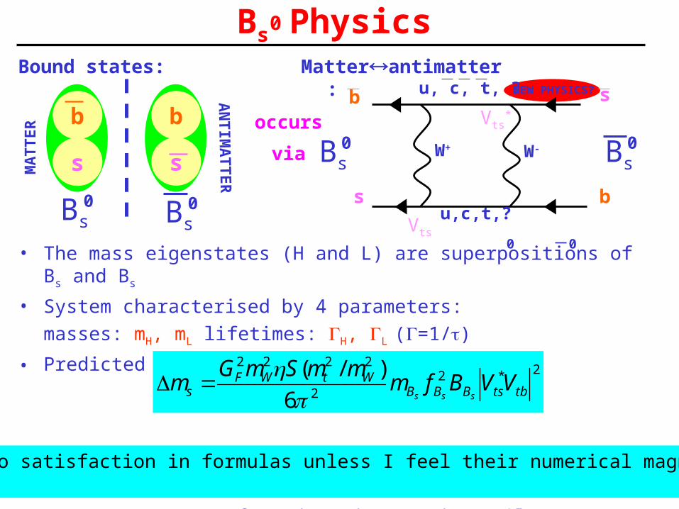
Bs PhysicsBound states:
b
s
b
s
Bs0 Bs
0
MATTER
ANTIM
ATTER
Matterantimatter:
0
• The mass eigenstates (H and L) are superpositions of Bs and Bs
• System characterised by 4 parameters:
masses: mH, mL lifetimes: H, L (=1/)
• Predicted ms around 20ps-1
• No measurements of ms have been made until now:
• B factories do not produce Bs Mesons
• Limits set by LEP, SLD, Tevatron
0 0
b s
s b
u, c, t, ?
u,c,t,?
Bs0 Bs
0W+ W-
NEW PHYSICS?
occurs
via
Vts
Vts*
2*22
2222
6
)/(tbtsBBB
WtWFs VVBfm
mmSmGm
sss
"I have no satisfaction in formulas unless I feel their numerical magnitude." (Kelvin)

from md
from md/ms
Lower limit on ms
4
Why is ms interesting?
1) Probe of New Physics - may enter in box diagrams
2) Measure CKM matrix element:
md known accurately from B factories• Vtd known to 15%• Ratio Vtd/Vts md/ms related by constants:
• (from lattice QCD) known to ~4%
• So: measure ms gives Vts
Standard Model Predicts rate of mixing, m=mH-mL, so Measure rate of mixing Vts (or hints of NEW physics)
2
2
2
td
ts
B
B
d
s
V
V
m
m
m
m
d
s
CKM Fit result: ms: 18.3+6.5 (1) ps-1

5
Measuring ms
mttBBNtBBN
tBBNtBBNtA
ssss
ssss
cos
))(())((
))(())(()(
0000
0000
In principle: Measure asymmetry of number of matter and antimatter decays:
In practice: m is measured by more complex techniques: amplitude scan and likelihood profile
H. G. Moser, A. Roussarie, NIM A384 (1997)
tmADeP
tmADeP
s
t
BB
mix
s
t
BB
unmix
sB
s
s
sB
s
s
cos12
1
cos12
1
Test Case: B0
d mixing
6
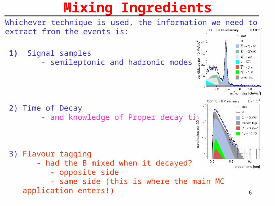
Mixing Ingredients
1) Signal samples - semileptonic and hadronic modes
2) Time of Decay - and knowledge of Proper decay time resolution
3) Flavour tagging - had the B mixed when it decayed? - opposite side - same side (this is where the main MC application enters!)
Whichever technique is used, the information we need to extract from the events is:
7
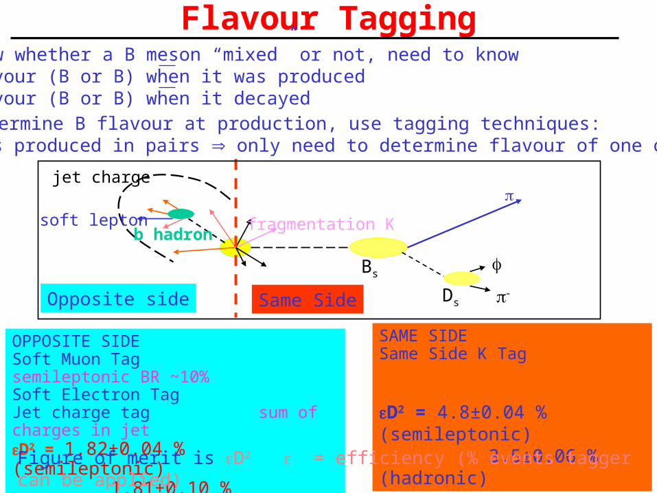
Flavour Tagging
To determine B flavour at production, use tagging techniques:b quarks produced in pairs only need to determine flavour of one of them
jet charge
soft leptonb hadron
fragmentation K
Bs
Ds
Opposite side Same Side
To know whether a B meson “mixed” or not, need to know1) flavour (B or B) when it was produced2) flavour (B or B) when it decayed
SAME SIDESame Side K Tag
D2 = 4.8±0.04 %(semileptonic) 3.5±0.06 % (hadronic)
OPPOSITE SIDESoft Muon Tag semileptonic BR ~10%Soft Electron TagJet charge tag sum of charges in jet D2 = 1.82±0.04 % (semileptonic) 1.81±0.10 % (hadronic)Figure of merit is D2 = efficiency (% events tagger can be applied) D = dilution (% events tagger is correct)
8
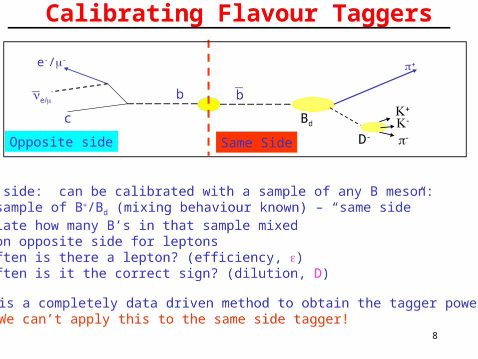
Calibrating Flavour Taggers
e-/-
Bd
D- Opposite side
Opposite side: can be calibrated with a sample of any B meson:1) Take sample of B+/Bd (mixing behaviour known) – “same side”2) Calculate how many B’s in that sample mixed3) Look on opposite side for leptons4) How often is there a lepton? (efficiency, )5) How often is it the correct sign? (dilution, D)
b b
c
This is a completely data driven method to obtain the tagger power BUT! We can’t apply this to the same side tagger!
e
Same Side
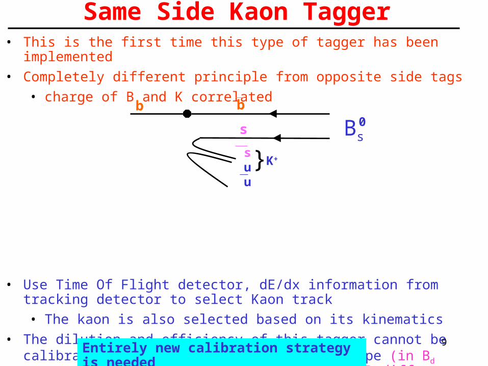
• This is the first time this type of tagger has been implemented
• Completely different principle from opposite side tags
• charge of B and K correlated
• Use Time Of Flight detector, dE/dx information from tracking detector to select Kaon track
• The kaon is also selected based on its kinematics
• The dilution and efficiency of this tagger cannot be calibrated independently of the B meson type (in Bd case, we would have a pion instead: pion ID different, fragmentation of Bd could be different)
9
Same Side Kaon Tagger
Bs0
s
b
s u u
K+}
b
Entirely new calibration strategy is needed
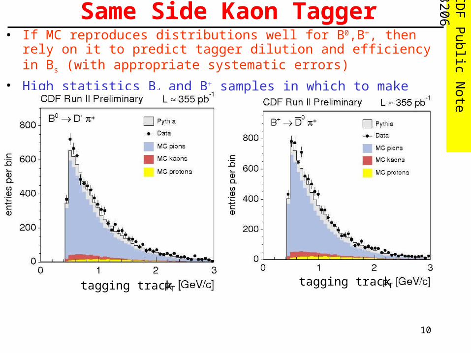
• If MC reproduces distributions well for B0,B+, then rely on it to predict tagger dilution and efficiency in Bs (with appropriate systematic errors)
• High statistics Bd and B+ samples in which to make data/MC comparisons:
• Compare e.g. transverse momentum distributions
• split into particle content (pions, kaons, protons)10
Same Side Kaon Tagger CD
F P
ublic N
ote
820
6
tagging track tagging track

• Then enhance kaon fraction by making selection on particle ID
• Check still get good comparison within available statistics
• (assign systematic error for this comparison)
11
Same Side Kaon Tagger
Two key points:1) this was not achieved by using “out of the box” Pythia 2) after finding a good comparison, most important to assign
systematic errors
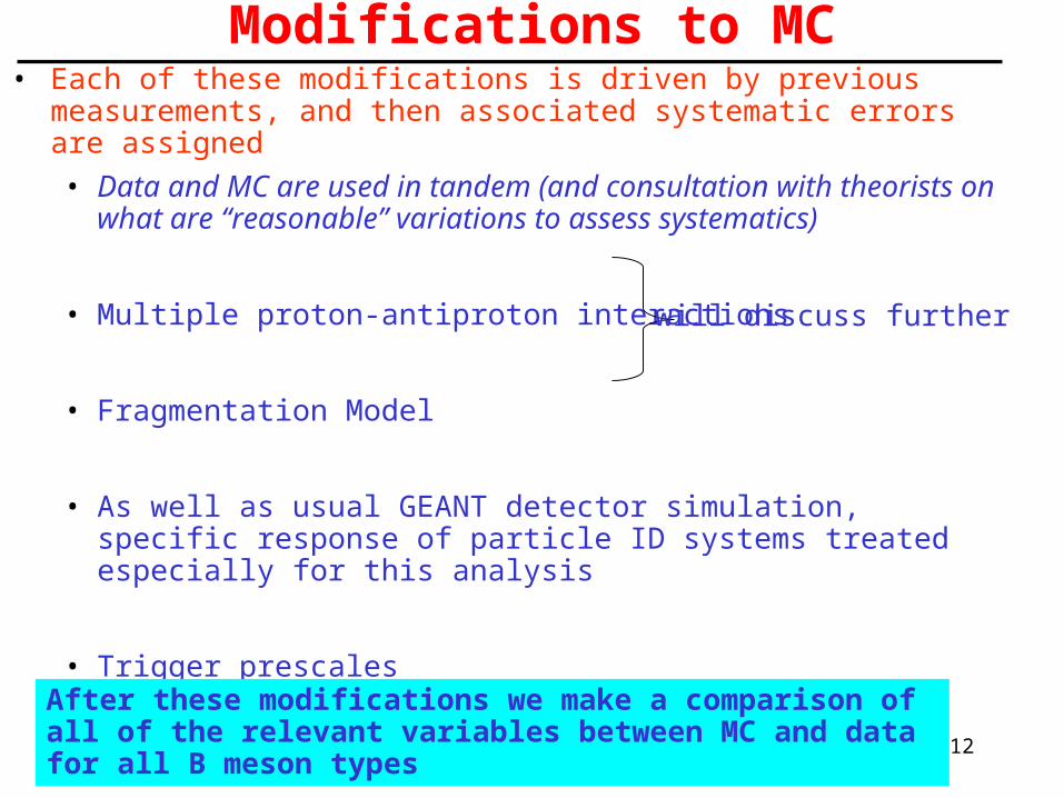
• Each of these modifications is driven by previous measurements, and then associated systematic errors are assigned
• Data and MC are used in tandem (and consultation with theorists on what are “reasonable” variations to assess systematics)
• Multiple proton-antiproton interactions
• Fragmentation Model
• As well as usual GEANT detector simulation, specific response of particle ID systems treated especially for this analysis
• Trigger prescales
12
Modifications to MC
After these modifications we make a comparison of all of the relevant variables between MC and data for all B meson types
will discuss further
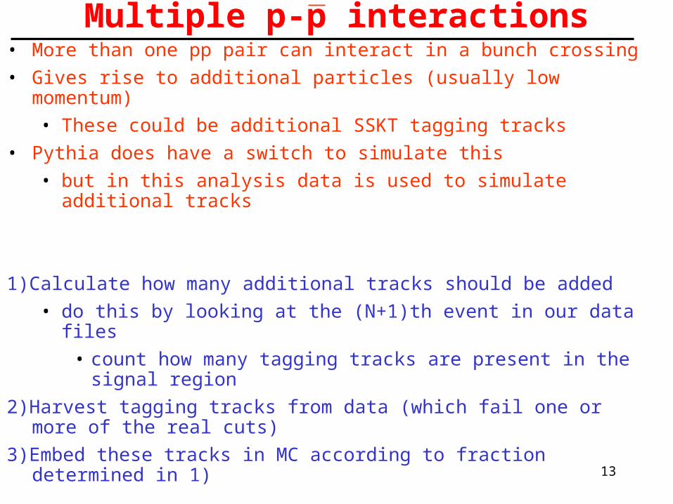
• More than one pp pair can interact in a bunch crossing
• Gives rise to additional particles (usually low momentum)
• These could be additional SSKT tagging tracks
• Pythia does have a switch to simulate this
• but in this analysis data is used to simulate additional tracks
1)Calculate how many additional tracks should be added
• do this by looking at the (N+1)th event in our data files
• count how many tagging tracks are present in the signal region
2)Harvest tagging tracks from data (which fail one or more of the real cuts)
3)Embed these tracks in MC according to fraction determined in 1)
13
Multiple p-p interactions
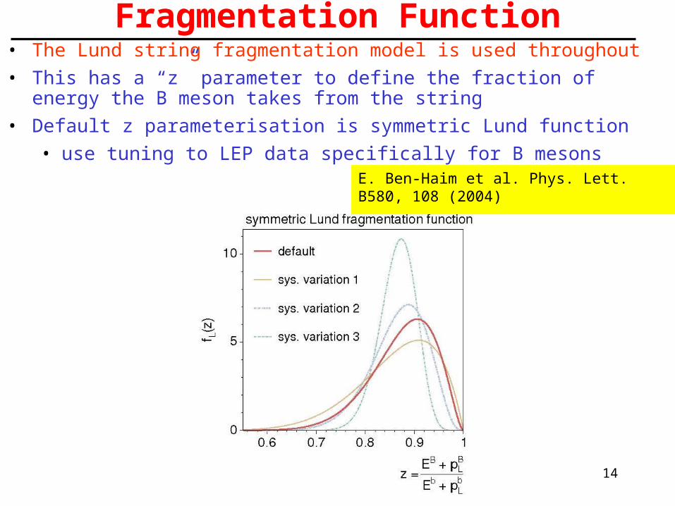
• The Lund string fragmentation model is used throughout
• This has a “z” parameter to define the fraction of energy the B meson takes from the string
• Default z parameterisation is symmetric Lund function
• use tuning to LEP data specifically for B mesons
14
Fragmentation Function
E. Ben-Haim et al. Phys. Lett. B580, 108 (2004)

• After all the modifications we compare all relevant distributions including efficiency and dilution in data and MC for Bd, B+
15
Efficiency and Dilution in Data/MC
So we conclude that for Bd, B+ there is a good match between data and MC. Thus we can move to using MC only for the Bs case.
B+ Bd
(%) Eff Dil Eff Dil
Data 58.4±0.5 25.4±1.4 57.2±0.6 14.2±2.9
MC 55.9 ±0.1 24.5±0.3 56.6±0.1 12.9±0.4
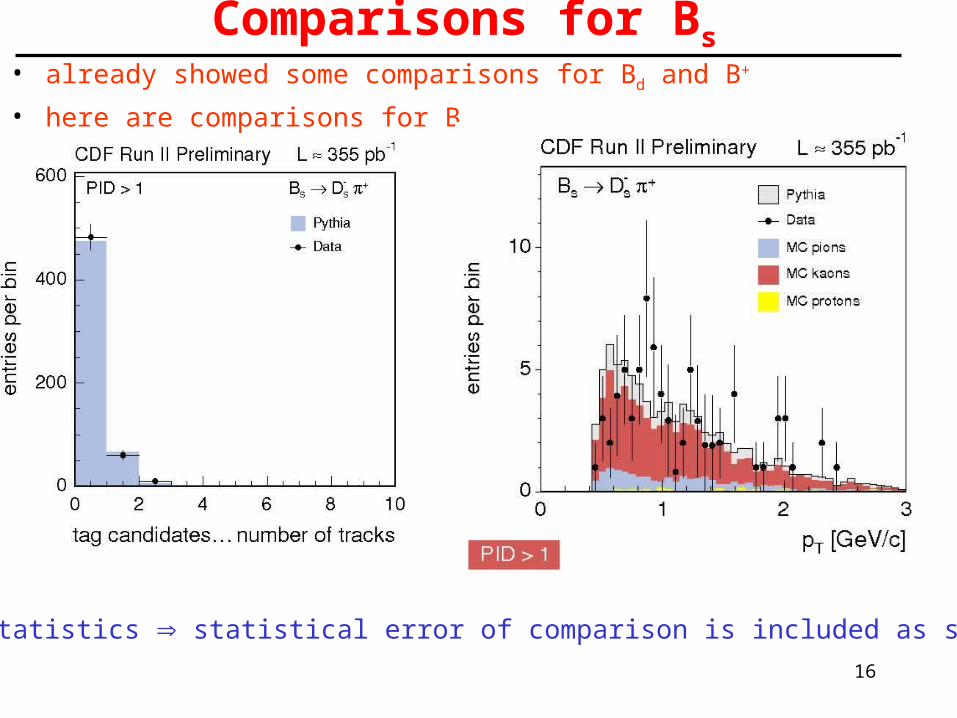
• already showed some comparisons for Bd and B+
• here are comparisons for Bs
16
Comparisons for Bs
Limited statistics statistical error of comparison is included as systematic error
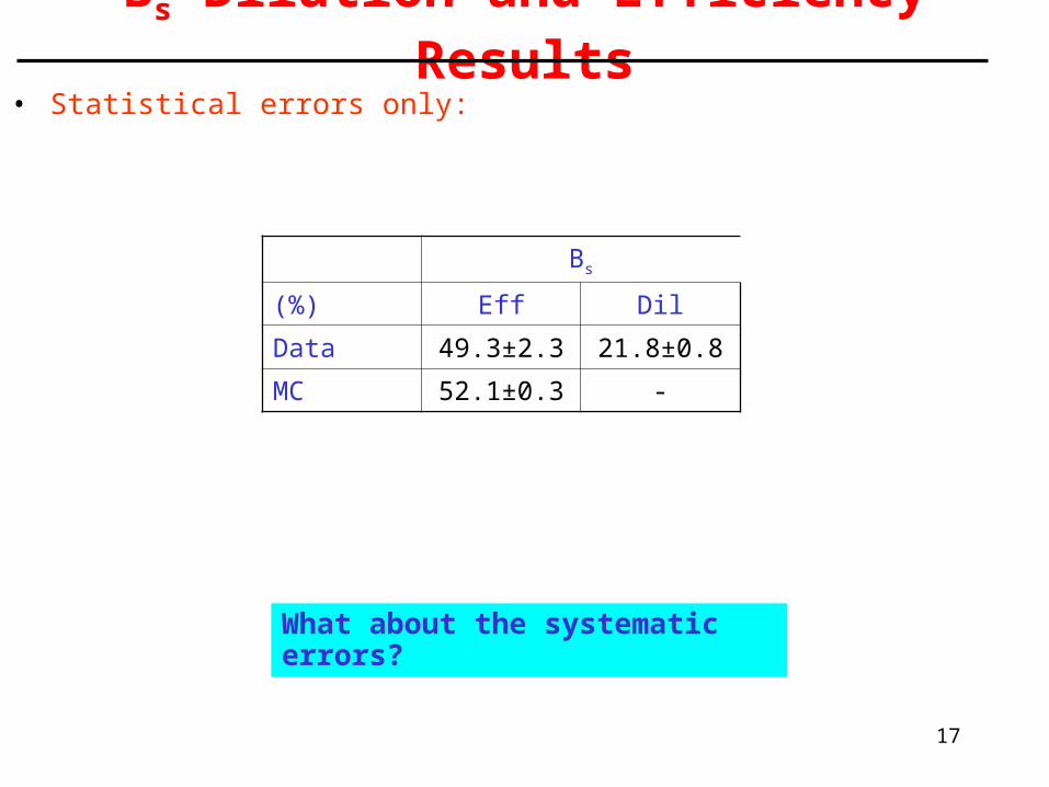
• Statistical errors only:
17
Bs Dilution and Efficiency Results
What about the systematic errors?
Bs
(%) Eff Dil
Data 49.3±2.3 21.8±0.8
MC 52.1±0.3 -

• A reminder of what we’ve done:
• modified MC
• checked that it compares well with data for Bd, B+
• compared efficiency and dilution for Bd, B+ from data and MC
• on the basis that they compare well, we extracted efficiency and dilution for Bs from MC
• To apply these numbers in our analysis we need a good understanding of the systematic errors
• Several sources:
• bb production mechanism
• fragmentation fraction
• particle content around the B
• variation within data statistics
• B** fraction
• particle ID detectors simulation
• pile-up18
Systematic Errors
will discuss further
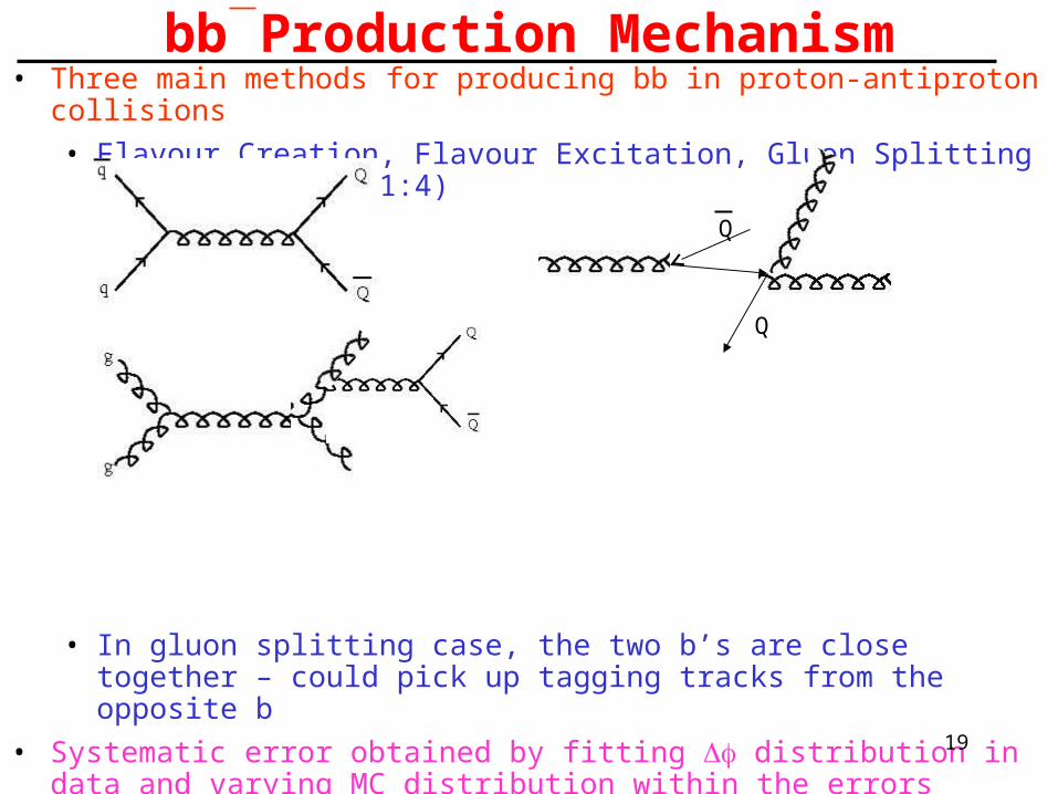
• Three main methods for producing bb in proton-antiproton collisions
• Flavour Creation, Flavour Excitation, Gluon Splitting (default mix 5:11:4)
• In gluon splitting case, the two b’s are close together – could pick up tagging tracks from the opposite b
• Systematic error obtained by fitting distribution in data and varying MC distribution within the errors
• This results in varying Gluon Splitting [-68%,+46%], Flavour Excitation and Creation [-50%,+50%]
19
bb Production Mechanism
Q
Q
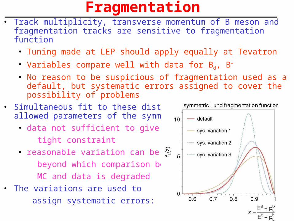
• Track multiplicity, transverse momentum of B meson and fragmentation tracks are sensitive to fragmentation function
• Tuning made at LEP should apply equally at Tevatron
• Variables compare well with data for Bd, B+
• No reason to be suspicious of fragmentation used as a default, but systematic errors assigned to cover the possibility of problems
• Simultaneous fit to these distributions to determine allowed parameters of the symmetric Lund function
• data not sufficient to give a
tight constraint
• reasonable variation can be obtained,
beyond which comparison between
MC and data is degraded
• The variations are used to
assign systematic errors:
20
Fragmentation
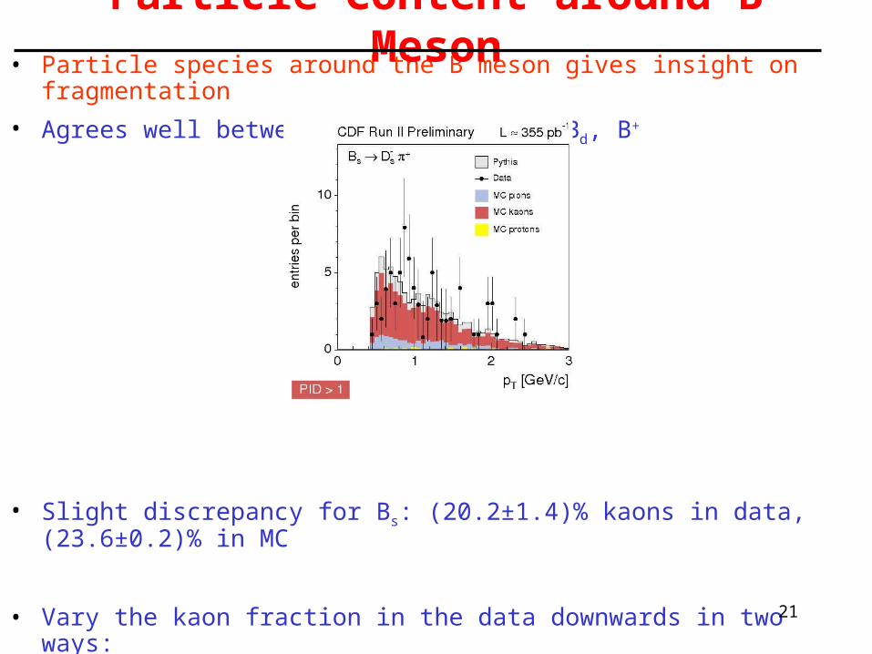
• Particle species around the B meson gives insight on fragmentation
• Agrees well between data and MC for Bd, B+
• Slight discrepancy for Bs: (20.2±1.4)% kaons in data, (23.6±0.2)% in MC
• Vary the kaon fraction in the data downwards in two ways:
• reweight all events with a kaon tagging track
• reweight only those events with prompt kaons from b-string21
Particle Content around B Meson
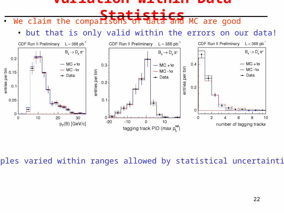
• We claim the comparisons of data and MC are good
• but that is only valid within the errors on our data!
22
Variation within Data Statistics
MC samples varied within ranges allowed by statistical uncertainties
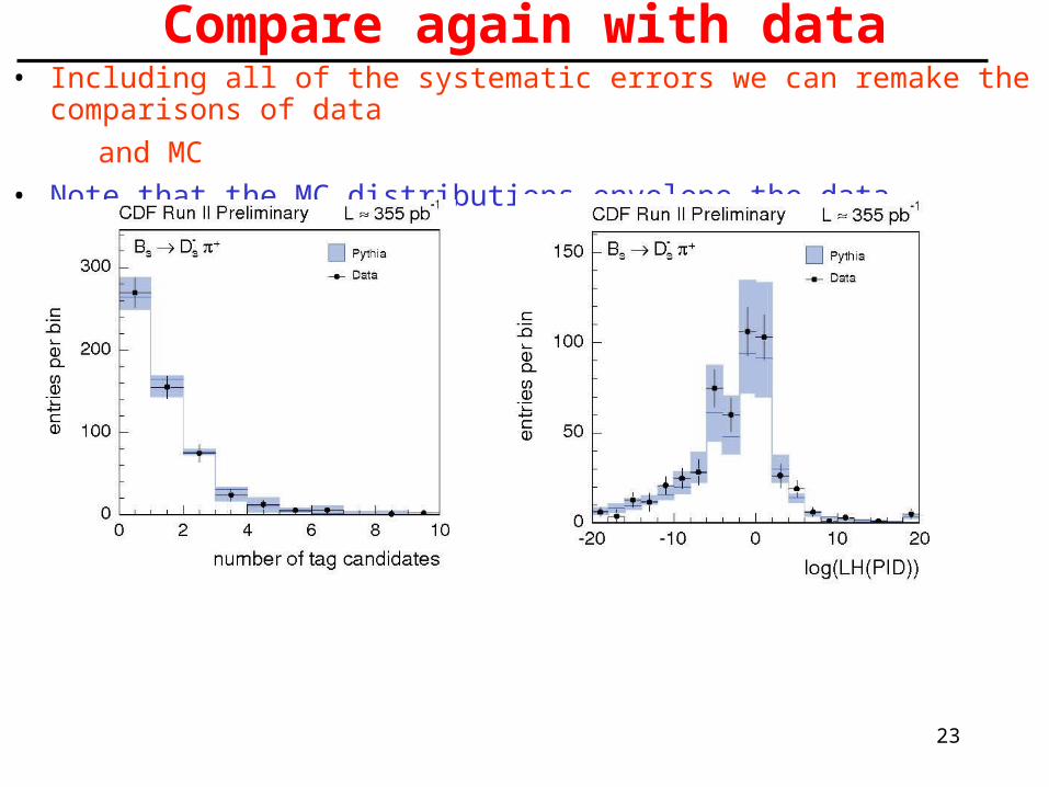
• Including all of the systematic errors we can remake the comparisons of data
and MC
• Note that the MC distributions envelope the data distributions
23
Compare again with data
24
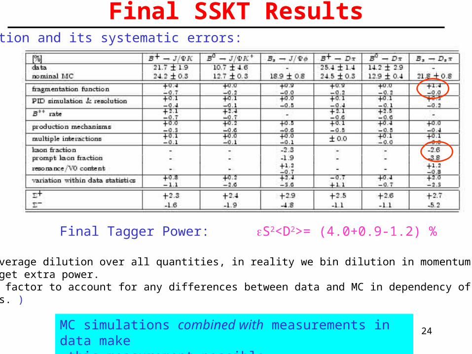
Final SSKT Results
Final Tagger Power: S2<D2>= (4.0+0.9-1.2) %(Notes: <D> is the average dilution over all quantities, in reality we bin dilution in momentum, particle IDvariable to get extra power.S is a scale factor to account for any differences between data and MC in dependency of dilution on variables. )
MC simulations combined with measurements in data make this measurement possible
Dilution and its systematic errors:
25
The Results
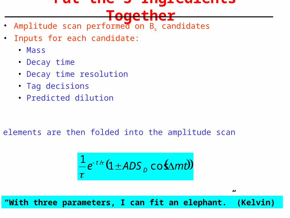
• Amplitude scan performed on Bs candidates
• Inputs for each candidate:
• Mass
• Decay time
• Decay time resolution
• Tag decisions
• Predicted dilution
26
Put the 3 Ingredients Together
• All elements are then folded into the amplitude scan
mtADSe Dt cos1
1 /
“With three parameters, I can fit an elephant.” (Kelvin)
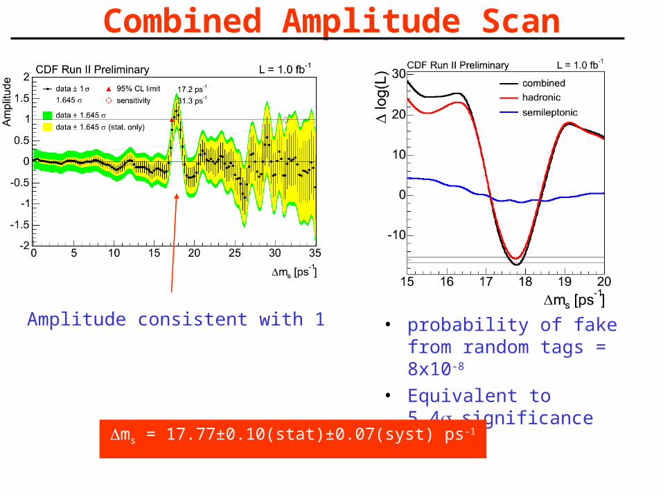
Combined Amplitude Scan
Amplitude consistent with 1 • probability of fake from random tags = 8x10⁻⁸
• Equivalent to 5.4significance
ms = 17.77±0.10(stat)±0.07(syst) ps-1
Conclusions
• CDF has found a signature consistent with Bs - Bs oscillations
– probability of this being a fluctuation is 8x10⁻⁸
• MC enabled the calibration of the most powerful flavour tagger– would not have been possible to such accuracy without experimental data to inform
the use of MC
• In my view the best (safest) possible way to use MC in analysis– use the data to make all possible checks
– use previous measurements, talk to theorists and use data itself to assign systematic errors for all of the unknowns
• Gives confidence in the results
ms = 17.77±0.10(stat)±0.07(syst) ps-1
Vts / Vtd= 0.2060 ± 0.0007 (exp) +0.0081 (theo) -0.0060
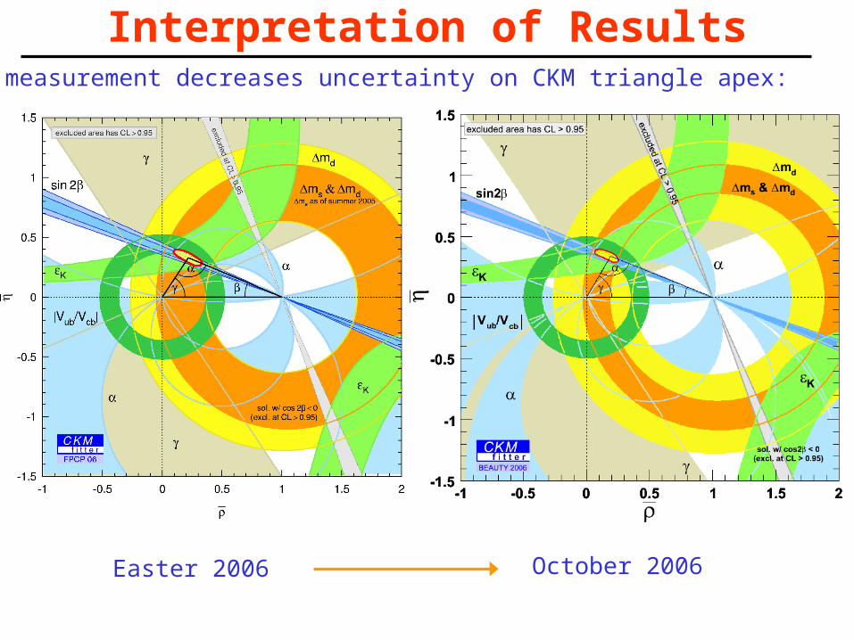
Interpretation of ResultsThis measurement decreases uncertainty on CKM triangle apex:
Easter 2006 October 2006
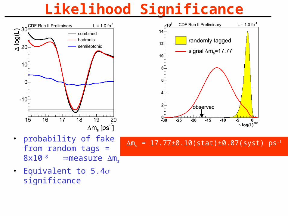
Likelihood Significance
• probability of fake from random tags = 8x10⁻⁸ measure ms
• Equivalent to 5.4 significance
ms = 17.77±0.10(stat)±0.07(syst) ps-1
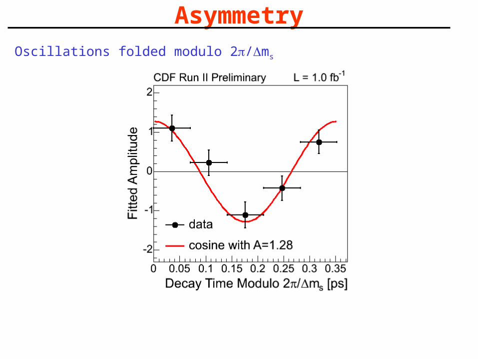
AsymmetryOscillations folded modulo 2/ms

• Can extract Vts value
• compare to Belle bs (hep-ex/050679):
|Vtd| / |Vts| = 0.199 +0.026 (exp) +0.018 (theo)
• our result:
|Vtd| / |Vts| = 0.2060 ± 0.0007 (exp) +0.0081 (theo)
|Vts| / |Vtd|
• inputs:• m(B0)/m(Bs) = 0.9832 (PDG 2006)• = 1.21 +0.05 (Lattice 2005)• md = 0.507±0.005 (PDG 2006)
-0.04
-0.0060
-0.025 -0.016
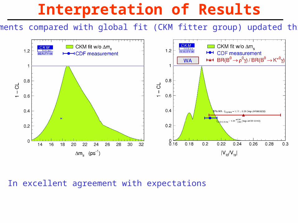
Interpretation of ResultsMeasurements compared with global fit (CKM fitter group) updated this month
In excellent agreement with expectations
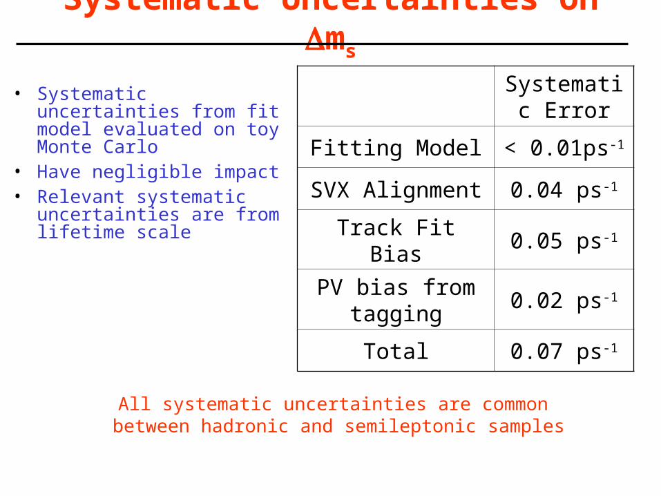
Systematic Uncertainties on ms
• Systematic uncertainties from fit model evaluated on toy Monte Carlo
• Have negligible impact• Relevant systematic
uncertainties are from lifetime scale
Systematic Error
Fitting Model < 0.01ps-1
SVX Alignment 0.04 ps-1
Track Fit Bias 0.05 ps-1
PV bias from tagging
0.02 ps-1
Total 0.07 ps-1
All systematic uncertainties are common between hadronic and semileptonic samples
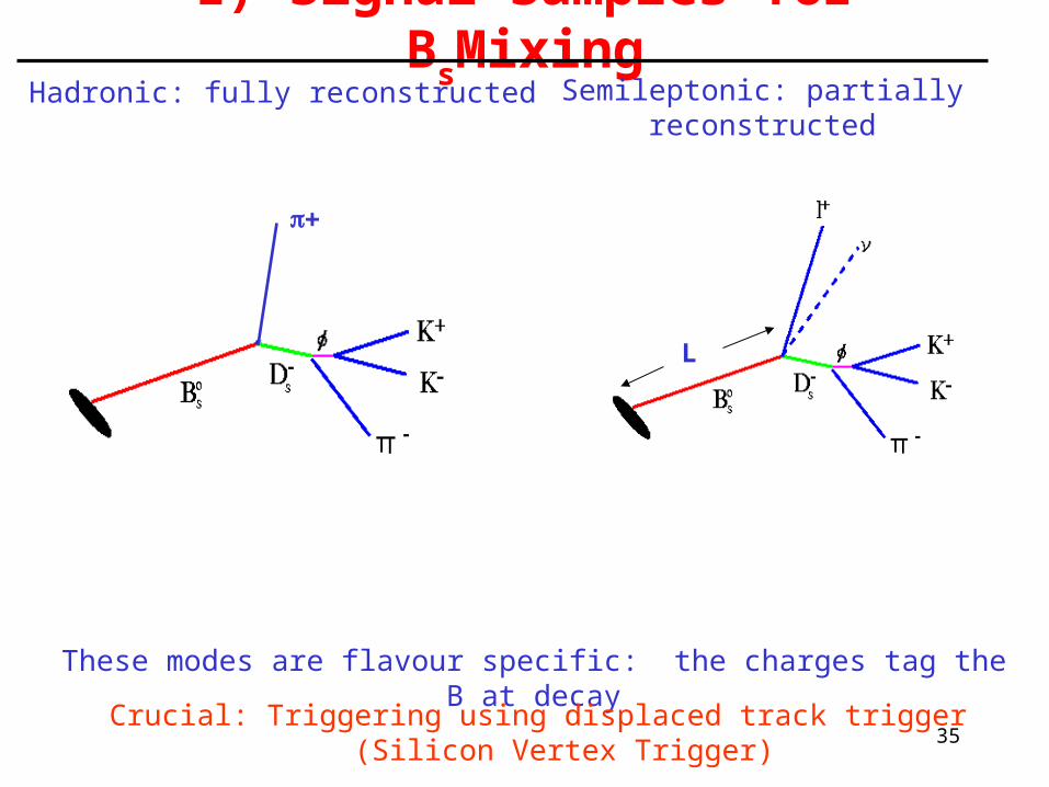
1) Signal Samples for BsMixing
35
L
Semileptonic: partially reconstructed
These modes are flavour specific: the charges tag the B at decay
Hadronic: fully reconstructed
Crucial: Triggering using displaced track trigger (Silicon Vertex Trigger)
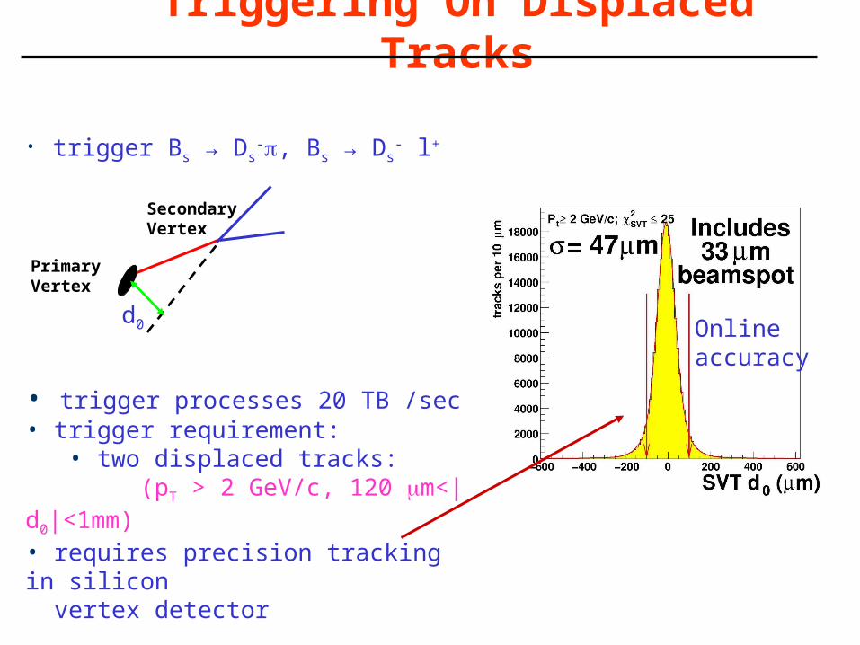
Triggering On Displaced Tracks
• trigger Bs → Ds-, Bs → Ds
- l+
• trigger processes 20 TB /sec• trigger requirement:
• two displaced tracks: (pT > 2 GeV/c, 120 m<|d0|<1mm)• requires precision tracking in silicon vertex detector
Primary Vertex
Secondary Vertex
d0 Onlineaccuracy

signalBs→ Ds, Ds → → K+K-
Example Hadronic Mass Spectrum
partiallyreconstructed
B mesons(satellites)
combinatorialbackground
B0→ D- decays
Previous mixing fit range
Now we use the entire range, capitalising on satellites also
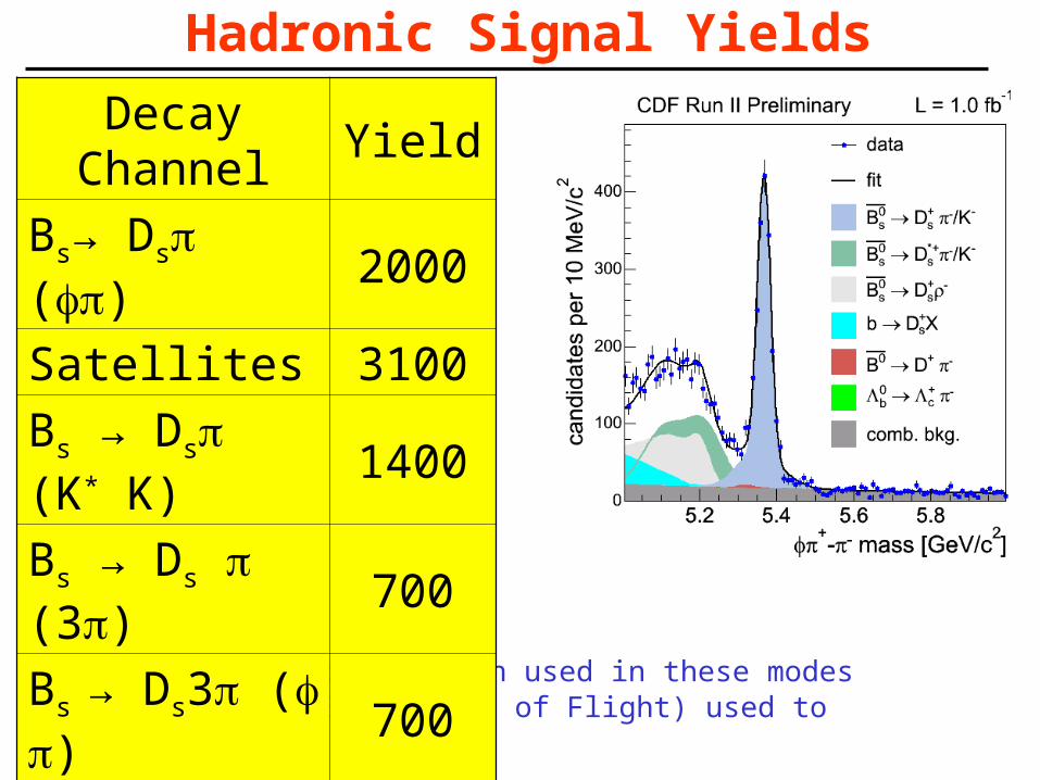
Hadronic Signal Yields
• Neural Network selection used in these modes• Particle ID (dE/dx, Time of Flight) used to suppress backgrounds
Decay Channel
Yield
Bs→ Ds () 2000
Satellites 3100
Bs → Ds (K* K)
1400
Bs → Ds (3) 700
Bs → Ds3 ( )
700
Bs → Ds3 (K*K)
600
Bs → Ds3 (3)
200
Total 8700
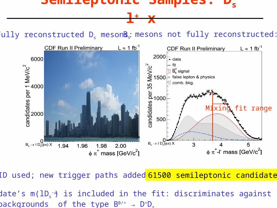
Semileptonic Samples: Ds- l+ x
Fully reconstructed Ds mesons: Bs mesons not fully reconstructed:
Particle ID used; new trigger paths added
The candidate’s m(lDs-) is included in the fit: discriminates against
“physics backgrounds” of the type B0/+ → D+Ds
Mixing fit range
61500 semileptonic candidates
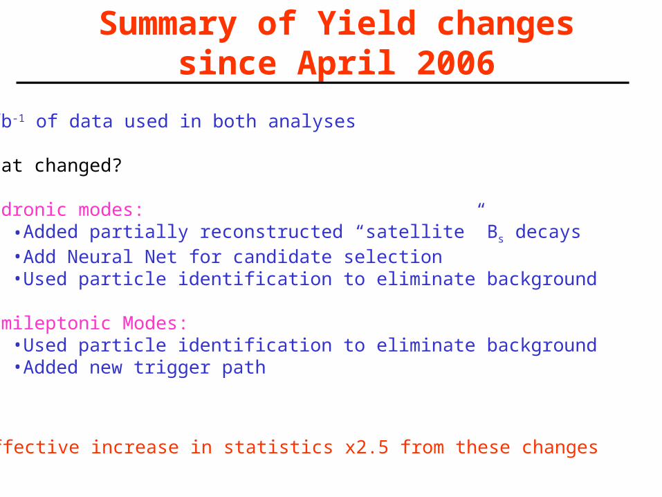
Summary of Yield changes since April 2006
1fb-1 of data used in both analyses
What changed?
Hadronic modes:•Added partially reconstructed “satellite” Bs decays•Add Neural Net for candidate selection•Used particle identification to eliminate background
Semileptonic Modes:•Used particle identification to eliminate background•Added new trigger path
Effective increase in statistics x2.5 from these changes
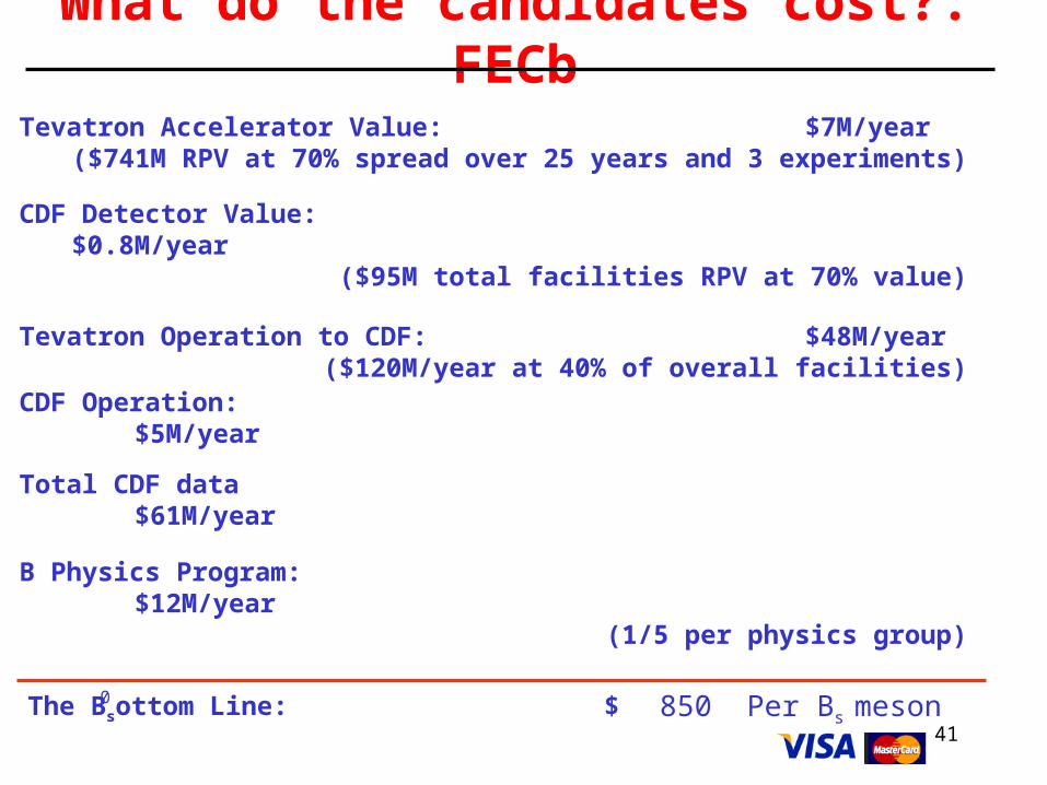
B Physics Program: $12M/year (1/5 per physics group)
41
What do the candidates cost?: FECb
Tevatron Accelerator Value: $7M/year ($741M RPV at 70% spread over 25 years and 3 experiments)
CDF Detector Value: $0.8M/year ($95M total facilities RPV at 70% value)
Tevatron Operation to CDF: $48M/year ($120M/year at 40% of overall facilities)
CDF Operation: $5M/year
Total CDF data $61M/year
The Bsottom Line: $0 850 Per Bs meson

42
• Reconstruct decay length by vertexing• Measure pT of decay products
K
lDp
BmL
Bp
BmL
Lct
T
xy
)()(
)(
2) Time of Decay
%0/
300
p
m
p
ct
2
20
pct p
ctct
%15/
590
p
m
p
ct
osc. period at ms = 18 ps-1
Crucial: Vertex resolution (Silicon Vertex Detector, in particular Layer00 very close to beampipe)
Hadronic:Semileptonic:
Proper time resolution:

Layer 00
• layer of silicon placed directly on beryllium beam pipe• Radius of 1.5 cm• additional impact parameter resolution
I.P resolutionwithout L00
• So-called because we already had layer 0 when this device was designed!• UK designed, built and (mostly) paid for this detector!
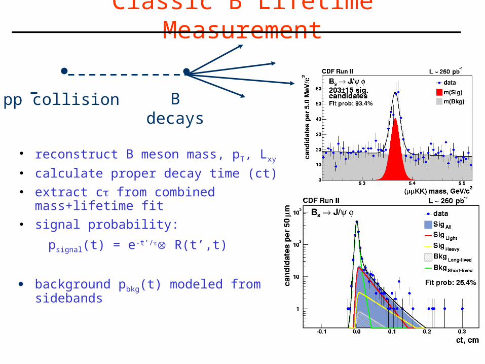
Classic B Lifetime Measurement
• reconstruct B meson mass, pT, Lxy
• calculate proper decay time (ct)
• extract c from combined mass+lifetime fit
• signal probability:
psignal(t) = e-t’/ R(t’,t)
● background pbkg(t) modeled from sidebands
pp collision B decays

Hadronic Lifetime Measurement
• Displaced track trigger biases the lifetime distribution
• Correct with an
efficiency function derived from MC:
p = e-t’/ R(t’,t) (t)
0.0 0.2 0.4proper time (cm)
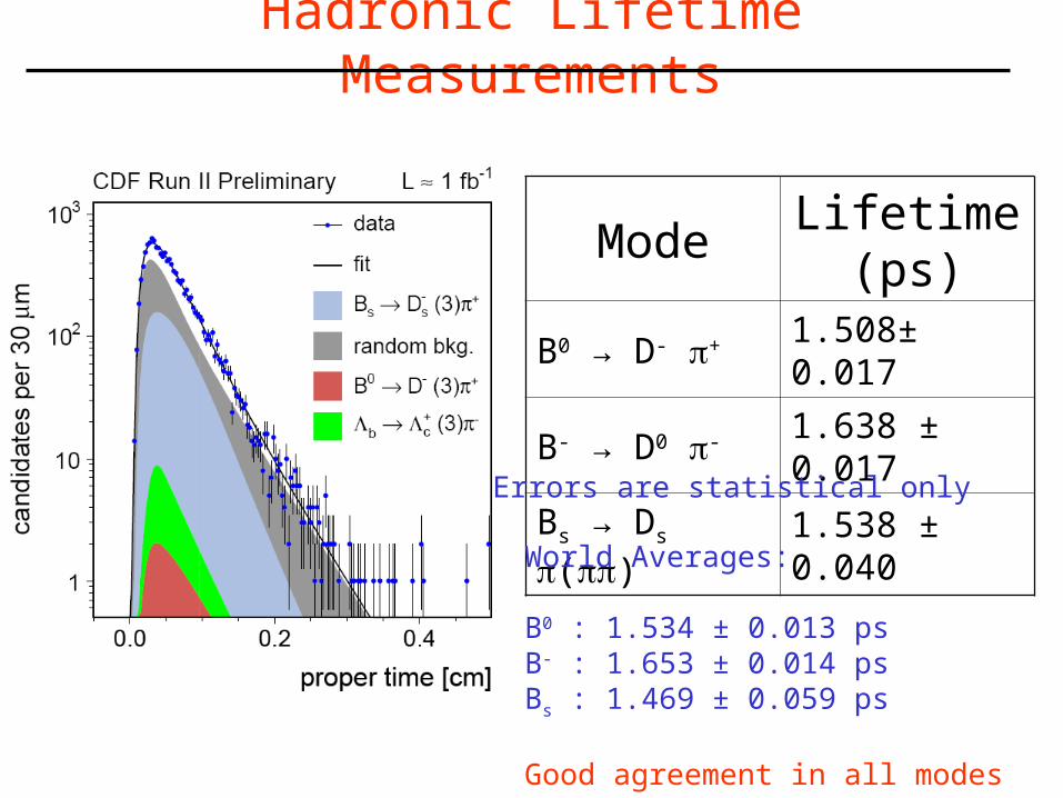
ModeLifetime
(ps)B0 → D- + 1.508± 0.017
B- → D0 - 1.638 ± 0.017
Bs → Ds () 1.538 ± 0.040
World Averages:
B0 : 1.534 ± 0.013 psB- : 1.653 ± 0.014 psBs : 1.469 ± 0.059 ps
Good agreement in all modes
Hadronic Lifetime Measurements
Errors are statistical only
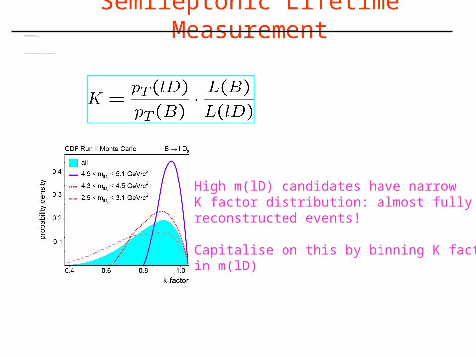
Semileptonic Lifetime Measurement• neutrino momentum missing
• Correct with “K factor” from MC:
• Also correct for displaced track trigger bias as in hadronic case
High m(lD) candidates have narrow K factor distribution: almost fullyreconstructed events!
Capitalise on this by binning K factorin m(lD)
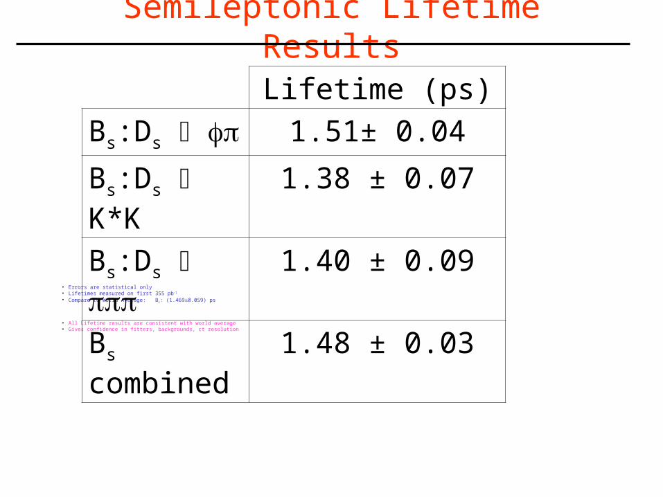
Semileptonic Lifetime Results
• Errors are statistical only• Lifetimes measured on first 355 pb-1 • Compare to World Average: Bs: (1.469±0.059) ps
• All Lifetime results are consistent with world average• Gives confidence in fitters, backgrounds, ct resolution
Lifetime (ps)
Bs:Ds 1.51± 0.04
Bs:Ds K*K 1.38 ± 0.07
Bs:Ds 1.40 ± 0.09
Bs combined
1.48 ± 0.03
49
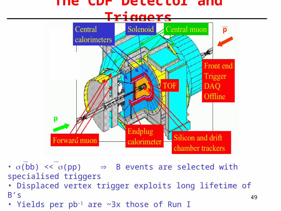
The CDF Detector and Triggers
• (bb) << (pp) B events are selected with specialised triggers• Displaced vertex trigger exploits long lifetime of B’s• Yields per pb-1 are ~3x those of Run I
p
p
50
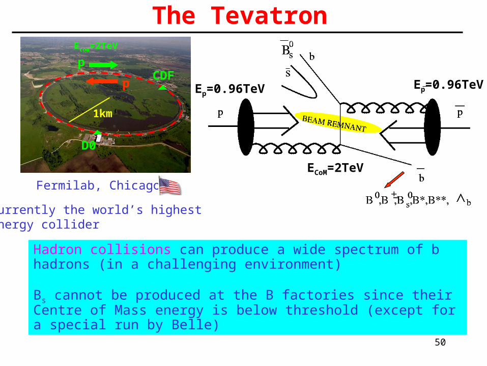
The Tevatron
Fermilab, Chicago
-
Currently the world’s highest energy collider
CDF
D0
p
p
1km
Ecom=2TeV
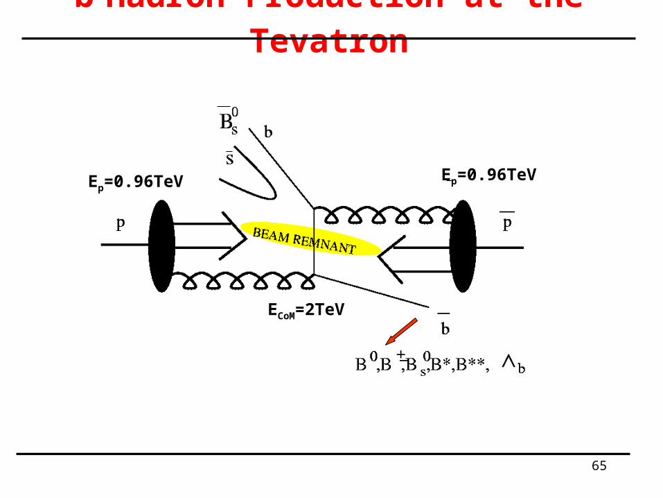
Hadron collisions can produce a wide spectrum of b hadrons (in a challenging environment)
Bs cannot be produced at the B factories since their Centre of Mass energy is below threshold (except for a special run by Belle)
-
Ep=0.96TeV Ep=0.96TeV
ECoM=2TeV
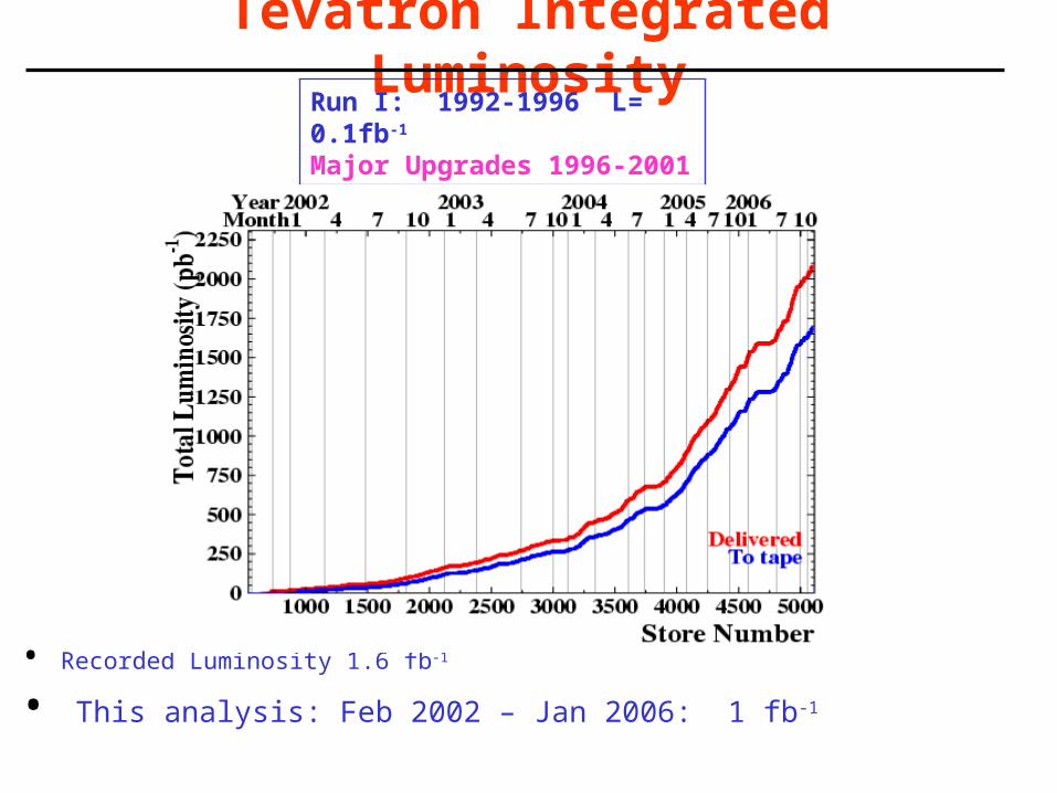
• This analysis: Feb 2002 – Jan 2006: 1 fb-1
Tevatron Integrated LuminosityRun I: 1992-1996 L= 0.1fb-1
Major Upgrades 1996-2001Run II: 2001-2006 L= 1.6 fb-1
• Recorded Luminosity 1.6 fb-1
52
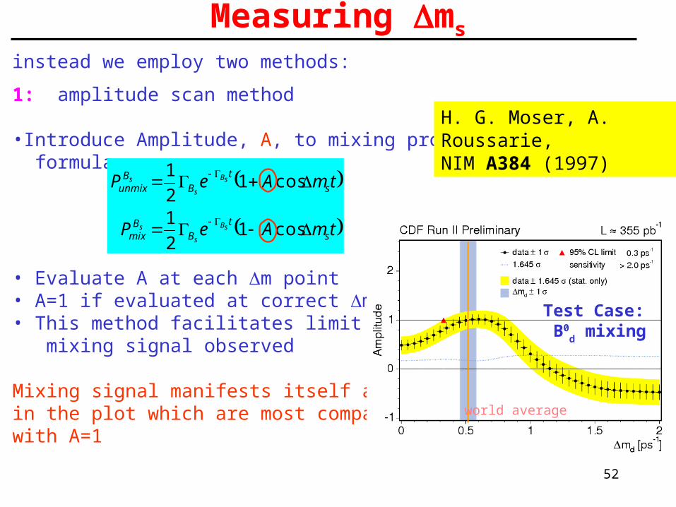
Measuring ms
1: amplitude scan method
•Introduce Amplitude, A, to mixing probability formula
• Evaluate A at each m point• A=1 if evaluated at correct m • This method facilitates limit setting before mixing signal observed
Mixing signal manifests itself as pointsin the plot which are most compatible with A=1
H. G. Moser, A. Roussarie, NIM A384 (1997)
Test Case: B0
d mixing
world average
tmAeP
tmAeP
s
t
BB
mix
s
t
BB
unmix
sB
s
s
sB
s
s
cos12
1
cos12
1
So instead we employ two methods:
53
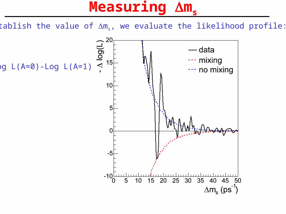
Measuring ms
2: To establish the value of ms, we evaluate the likelihood profile:
Log L(A=0)-Log L(A=1)
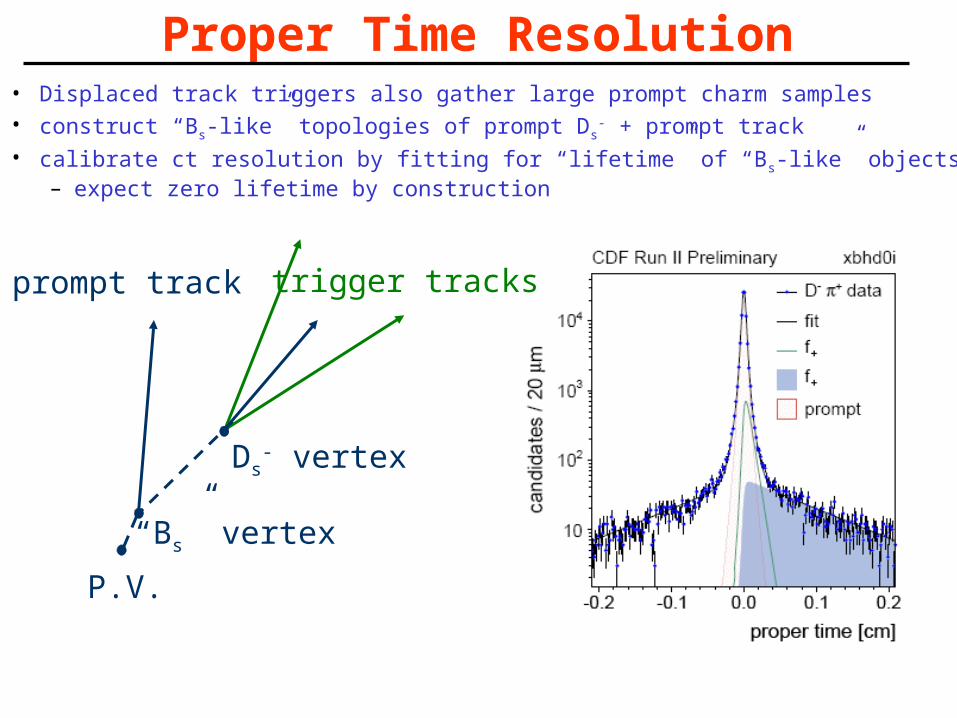
Proper Time Resolution• Displaced track triggers also gather large prompt charm samples• construct “Bs-like” topologies of prompt Ds
- + prompt track• calibrate ct resolution by fitting for “lifetime” of “Bs-like” objects
– expect zero lifetime by construction
trigger tracksprompt track
Ds- vertex
P.V.
“Bs” vertex
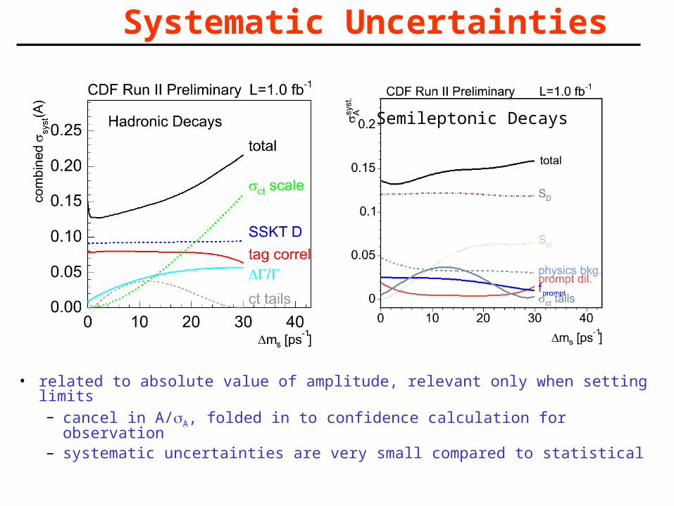
Systematic Uncertainties
• related to absolute value of amplitude, relevant only when setting limits – cancel in A/A, folded in to confidence calculation for observation– systematic uncertainties are very small compared to statistical
Semileptonic Decays
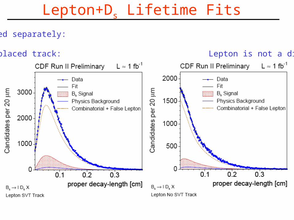
Lepton+Ds Lifetime Fits Two cases treated separately:
Lepton is a displaced track: Lepton is not a displaced track:
57
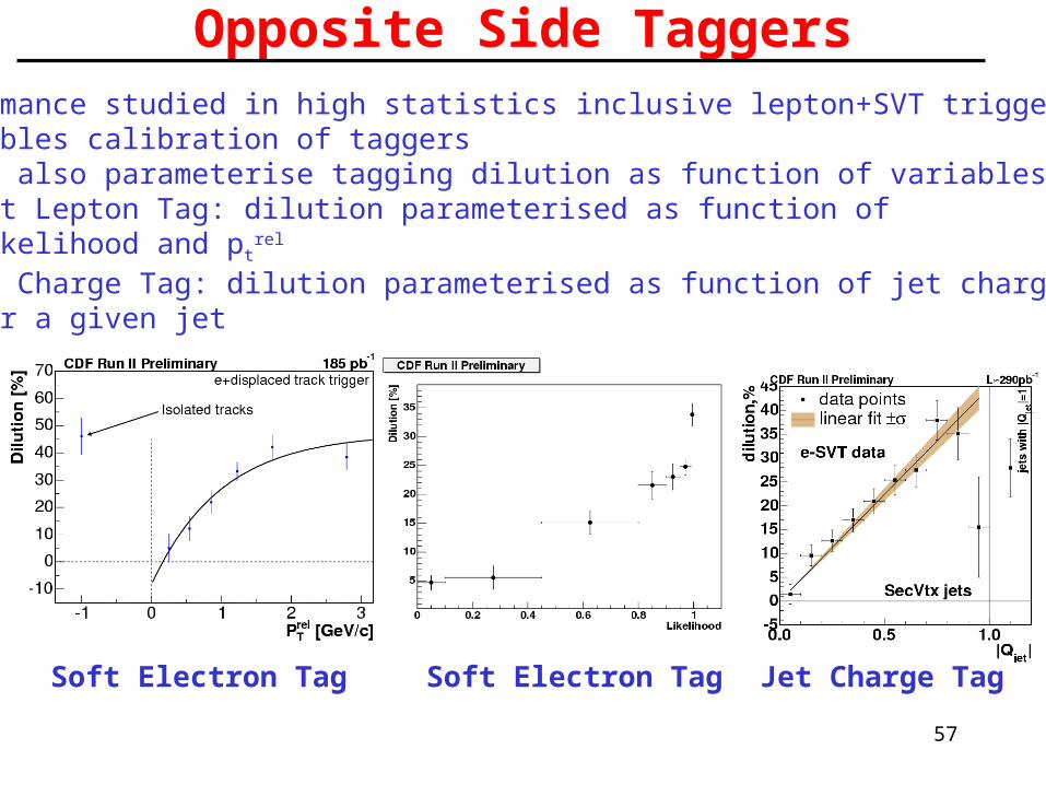
Opposite Side Taggers•Performance studied in high statistics inclusive lepton+SVT trigger
•Enables calibration of taggers•Can also parameterise tagging dilution as function of variables: •Soft Lepton Tag: dilution parameterised as function of likelihood and pt
rel
•Jet Charge Tag: dilution parameterised as function of jet charge for a given jet
Soft Electron Tag Soft Electron Tag Jet Charge Tag
58
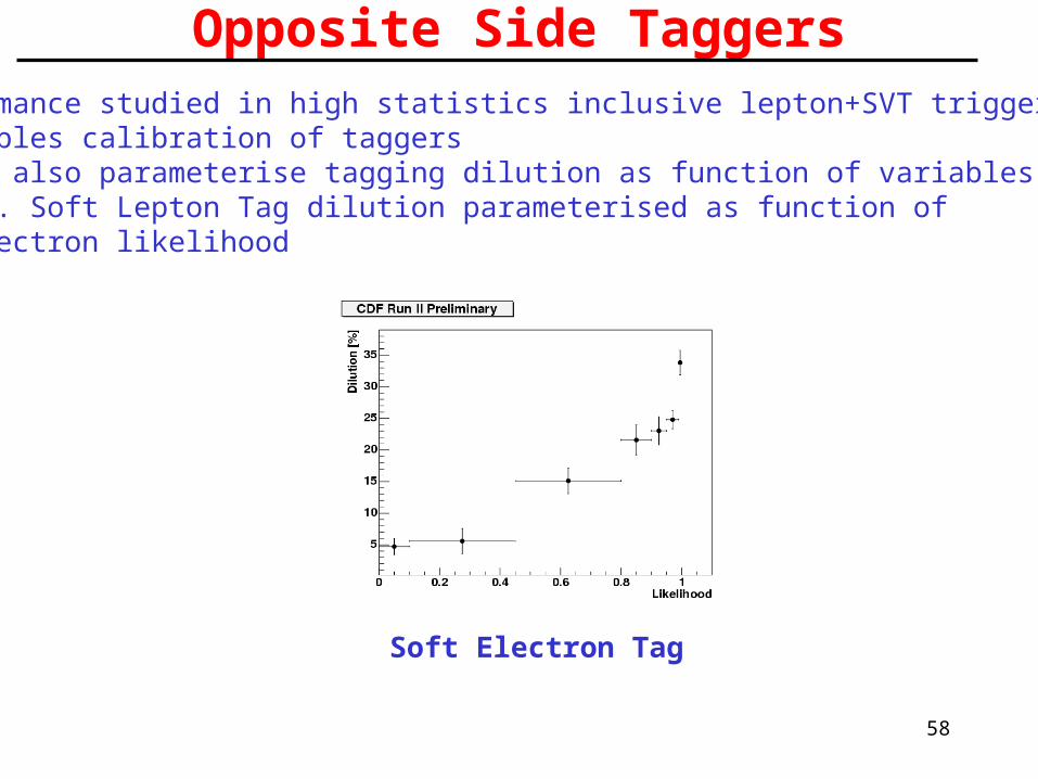
Opposite Side Taggers•Performance studied in high statistics inclusive lepton+SVT trigger
•Enables calibration of taggers•Can also parameterise tagging dilution as function of variables: •E.g. Soft Lepton Tag dilution parameterised as function of electron likelihood
Soft Electron Tag

59
Proper Time Resolution
osc. period at ms = 18 ps-1
• event by event determination of primary vertex position used
• average uncertainty
~ 26 m
• this information is used per candidate in the likelihood fit
• utilize large prompt charm cross section
• construct “Bs-like” topologies of prompt Ds- + prompt track
• calibrate ct resolution by fitting for “lifetime” of “Bs-like” objects
%15/
590
p
m
p
ct
%0/
300
p
m
p
ct
semileptonic: hadronic:
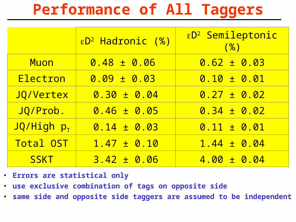
Performance of All Taggers
• Errors are statistical only
• use exclusive combination of tags on opposite side
• same side and opposite side taggers are assumed to be independent
D2 Hadronic (%) D2 Semileptonic (%)
Muon 0.48 ± 0.06 0.62 ± 0.03
Electron 0.09 ± 0.03 0.10 ± 0.01
JQ/Vertex 0.30 ± 0.04 0.27 ± 0.02
JQ/Prob. 0.46 ± 0.05 0.34 ± 0.02
JQ/High pT 0.14 ± 0.03 0.11 ± 0.01
Total OST 1.47 ± 0.10 1.44 ± 0.04
SSKT 3.42 ± 0.06 4.00 ± 0.04
61
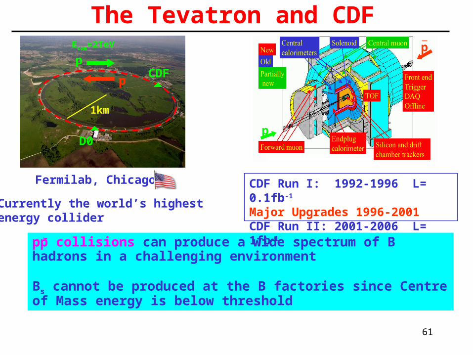
The Tevatron and CDF
Fermilab, Chicago
-
Currently the world’s highest energy collider
CDF
D0
p
p
1km
Ecom=2TeV
pp collisions can produce a wide spectrum of B hadrons in a challenging environment
Bs cannot be produced at the B factories since Centre of Mass energy is below threshold
p
p
CDF Run I: 1992-1996 L= 0.1fb-1
Major Upgrades 1996-2001CDF Run II: 2001-2006 L= 1fb-1
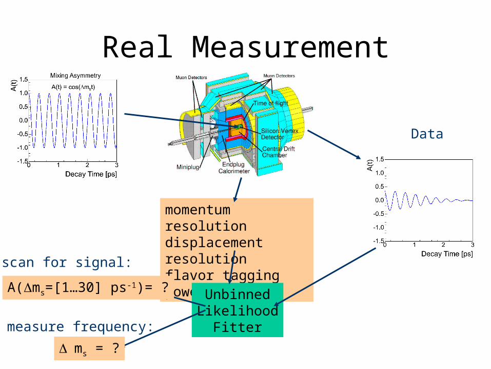
Real Measurement Layout
momentum resolutiondisplacement resolutionflavor tagging power
UnbinnedLikelihood
Fitter
Data
A(ms=[1…30] ps-1)= ?
ms = ?
scan for signal:
measure frequency:

The CDFII Detector• multi-purpose detector• excellent momentum
resolution (p)/p<0.1%
• Yield:– SVT based triggers
• Tagging power:– TOF, dE/dX in COT
• Proper time resolution:– SVXII, L00
64
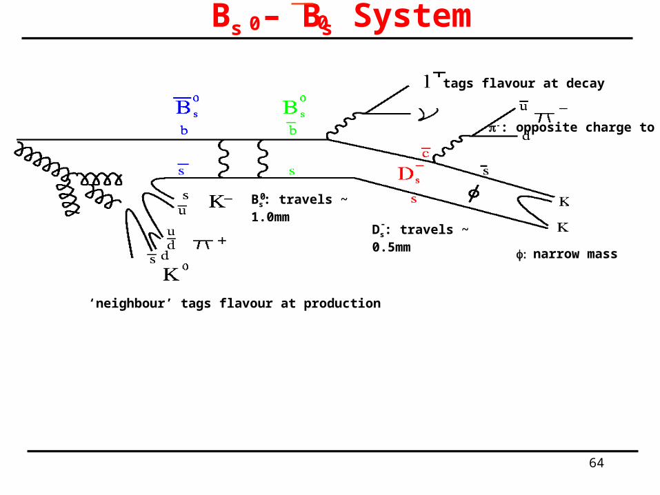
Bs – Bs System
tags flavour at decay
narrow mass
Bs: travels ~ 1.0mm
0
Ds: travels ~ 0.5mm
-
‘neighbour’ tags flavour at production
-: opposite charge to l+
0 0
65
-
Ep=0.96TeV Ep=0.96TeV
ECoM=2TeV
b Hadron Production at the Tevatron

66
Semileptonic Decay Fit ModelUnbinned maximum likelihood fit to c(B)
– Background is parameterised by delta function and positive exp convoluted with Gaussian resolution:
Free parameters: D E + f+ G
– Signal: exp convoluted with Gaussian resolution, K factor distribution, P(K), and bias function,
– Maximum likelihood function:
),(exp)(1 GE
Dbkg tGtf
tfF
)(),()(exp KPstGKtKt
cK
NF isig
bkgsig N
j
jbkg
N
i
ibkgbkg
isigbkg FFfFfL 1

67
• Reconstruct decay length by vertexing• Measure pT of decay products
K
lDp
BmL
Bp
BmL
Lct
T
xy
)()(
)(
2) Time of Decay
%0/
300
p
m
p
ct
•Displaced Track Trigger imposes bias correct with efficiency function
2
20
pct p
ctct
%15/
590
p
m
p
ct
osc. period at ms = 18 ps-1
Crucial: Vertex resolution (Silicon Vertex Detector, in particular Layer00 very close to beampipe)

68
Bs – Bs System
Want to understand: - Average lifetime,
- Lifetime difference, - Rate of mixing, m
Current Status: Experiment Theory
<0.29 0.15
m (ps-1) >14.1 20
0 0
2LH
LH
LH mm


