1

CS 430/536 Computer Graphics I

B-Splines and NURBS Week 5, Lecture 9

David Breen, William Regli and Maxim Peysakhov Geometric and Intelligent Computing Laboratory

Department of Computer Science Drexel University

http://gicl.cs.drexel.edu

2

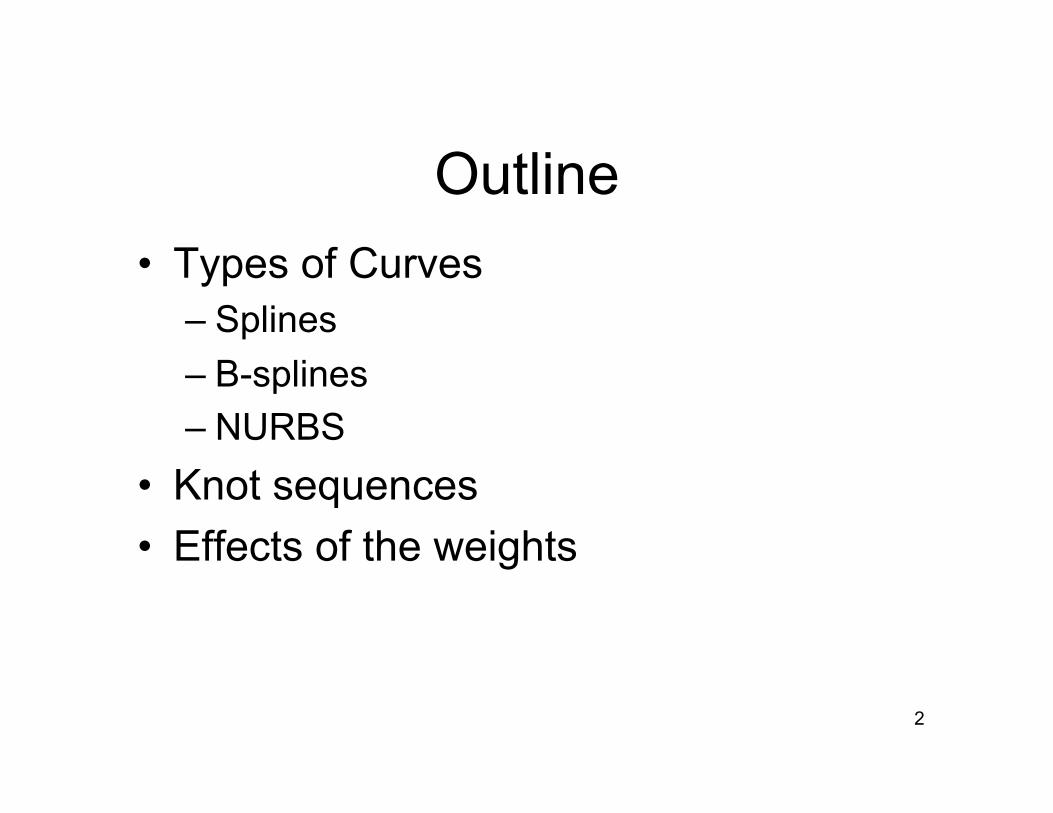
Outline •  Types of Curves

– Splines – B-splines – NURBS

•  Knot sequences •  Effects of the weights

3

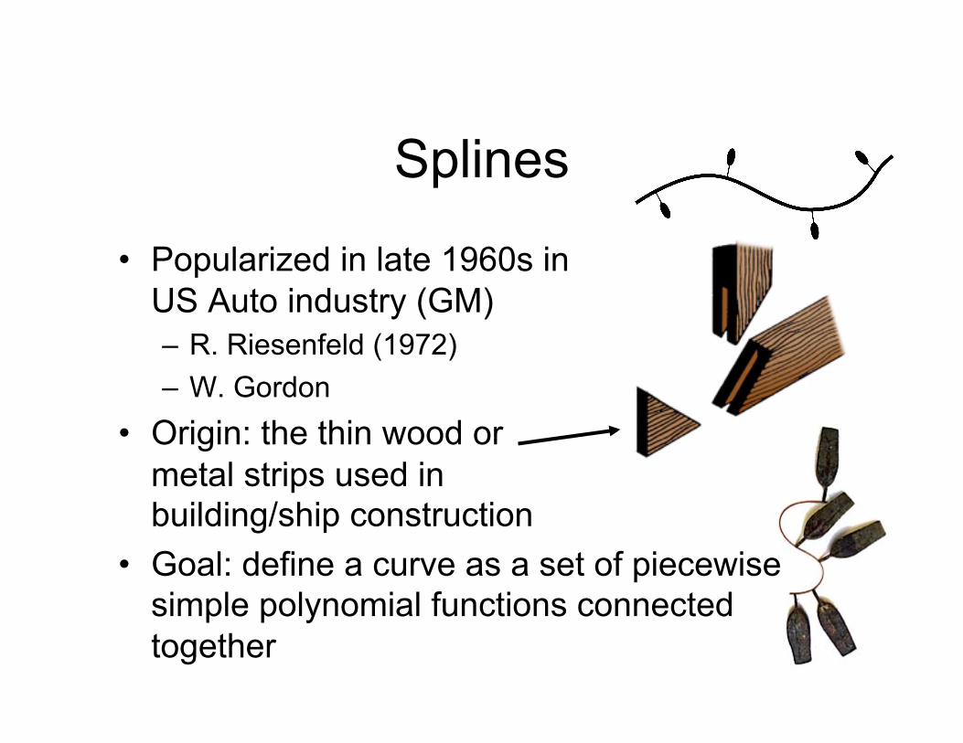
Splines

•  Popularized in late 1960s in US Auto industry (GM) –  R. Riesenfeld (1972) –  W. Gordon

•  Origin: the thin wood or metal strips used in building/ship construction

•  Goal: define a curve as a set of piecewise simple polynomial functions connected together

4

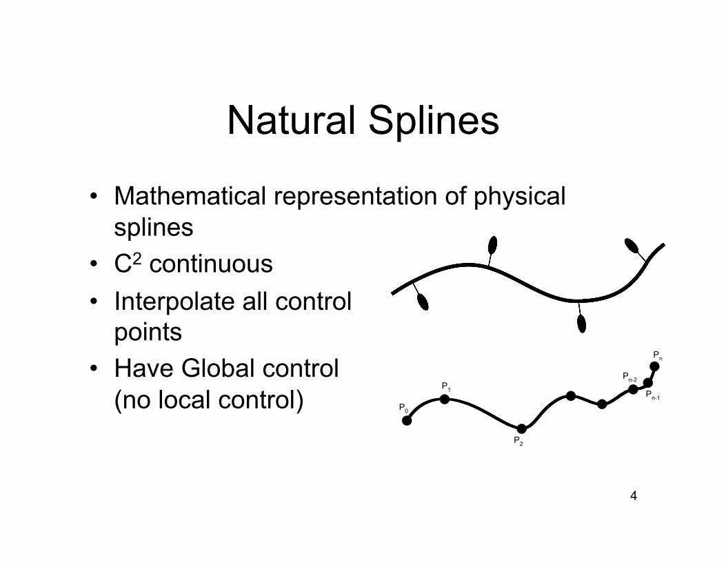
Natural Splines

•  Mathematical representation of physical splines

•  C2 continuous •  Interpolate all control

points •  Have Global control

(no local control) P0

P1

Pn

Pn-1

P2

Pn-2

5

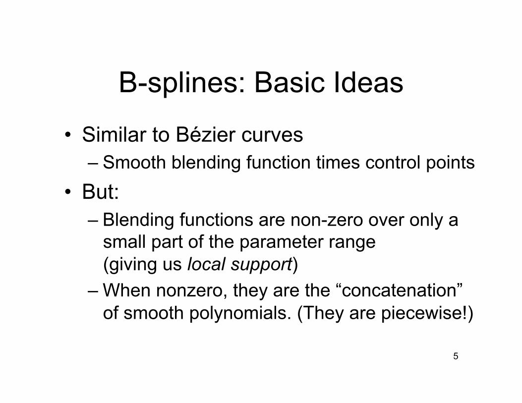
B-splines: Basic Ideas

•  Similar to Bézier curves – Smooth blending function times control points

•  But: – Blending functions are non-zero over only a

small part of the parameter range (giving us local support)

– When nonzero, they are the “concatenation” of smooth polynomials. (They are piecewise!)

6

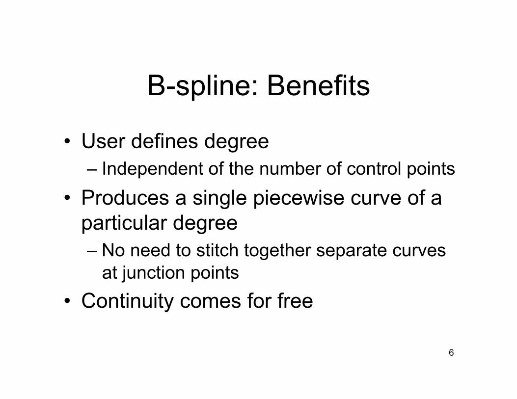
B-spline: Benefits

•  User defines degree –  Independent of the number of control points

•  Produces a single piecewise curve of a particular degree – No need to stitch together separate curves

at junction points •  Continuity comes for free

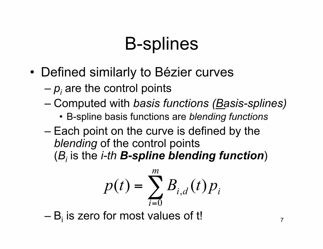
•  Defined similarly to Bézier curves – pi are the control points – Computed with basis functions (Basis-splines)

•  B-spline basis functions are blending functions – Each point on the curve is defined by the

blending of the control points (Bi is the i-th B-spline blending function)

– Bi is zero for most values of t!

∑=

=m

iidi ptBtp

0, )()(

7

B-splines

8

)()()(

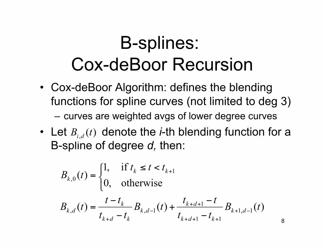
otherwise,0if,1

)(

1,111

11,,

10,

tBtttttB

tttttB

ttttB

dkkdk

dkdk

kdk

kdk

kkk

−++++

++−

+

+

−

−+

−

−=

<≤

=

B-splines: Cox-deBoor Recursion

•  Cox-deBoor Algorithm: defines the blending functions for spline curves (not limited to deg 3) –  curves are weighted avgs of lower degree curves

•  Let denote the i-th blending function for a B-spline of degree d, then:

)(, tB di

9

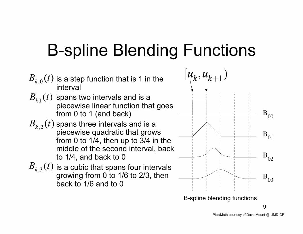
B-spline Blending Functions •  is a step function that is 1 in the

interval •  spans two intervals and is a

piecewise linear function that goes from 0 to 1 (and back)

•  spans three intervals and is a piecewise quadratic that grows from 0 to 1/4, then up to 3/4 in the middle of the second interval, back to 1/4, and back to 0

•  is a cubic that spans four intervals growing from 0 to 1/6 to 2/3, then back to 1/6 and to 0

Pics/Math courtesy of Dave Mount @ UMD-CP

B-spline blending functions

)(0, tBk

€

Bk,1(t)

)(2, tBk

)(3, tBk

10

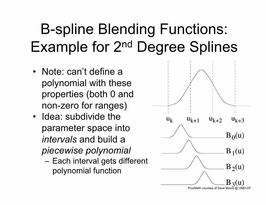
B-spline Blending Functions: Example for 2nd Degree Splines •  Note: can’t define a

polynomial with these properties (both 0 and non-zero for ranges)

•  Idea: subdivide the parameter space into intervals and build a piecewise polynomial –  Each interval gets different

polynomial function

Pics/Math courtesy of Dave Mount @ UMD-CP

11

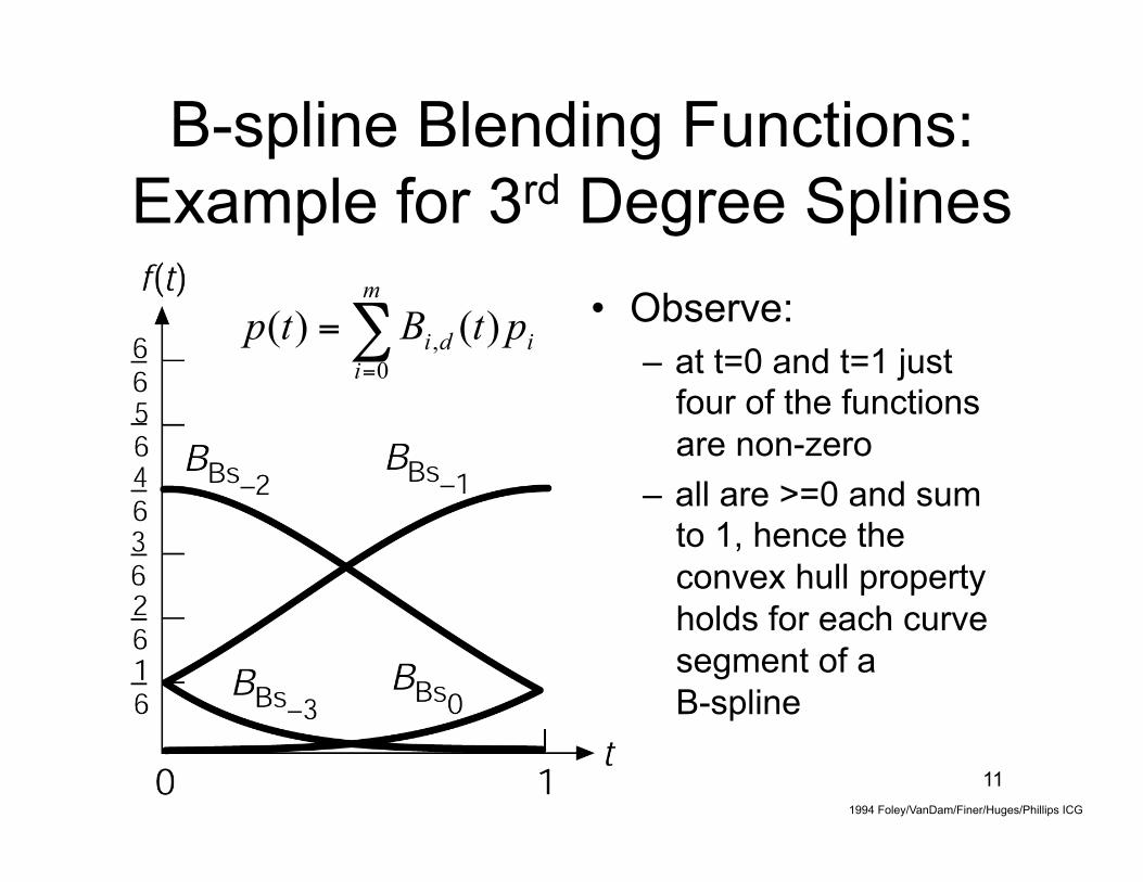
B-spline Blending Functions: Example for 3rd Degree Splines

•  Observe: –  at t=0 and t=1 just

four of the functions are non-zero

–  all are >=0 and sum to 1, hence the convex hull property holds for each curve segment of a B-spline

1994 Foley/VanDam/Finer/Huges/Phillips ICG

∑=

=m

iidi ptBtp

0, )()(

12

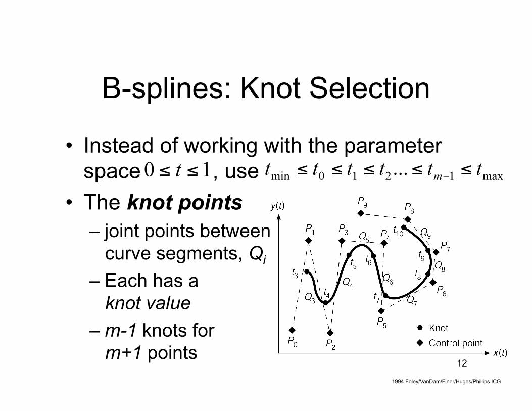
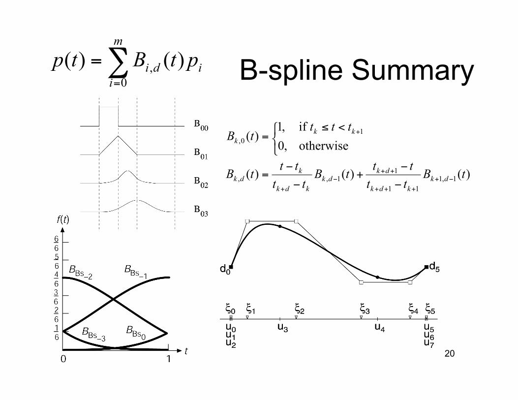
B-splines: Knot Selection

•  Instead of working with the parameter space , use

•  The knot points –  joint points between

curve segments, Qi – Each has a

knot value – m-1 knots for

m+1 points

10 ≤≤ t max1210min ... tttttt m ≤≤≤≤≤ −

1994 Foley/VanDam/Finer/Huges/Phillips ICG

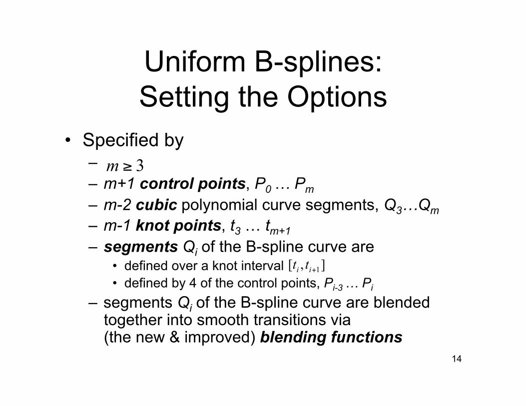
14

Uniform B-splines: Setting the Options

•  Specified by –  –  m+1 control points, P0 … Pm –  m-2 cubic polynomial curve segments, Q3…Qm –  m-1 knot points, t3 … tm+1 –  segments Qi of the B-spline curve are

•  defined over a knot interval •  defined by 4 of the control points, Pi-3 … Pi

–  segments Qi of the B-spline curve are blended together into smooth transitions via (the new & improved) blending functions

],[ 1+ii tt

3≥m

15

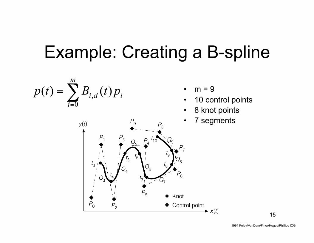
Example: Creating a B-spline

∑=

=m

iidi ptBtp

0, )()( •  m = 9

•  10 control points •  8 knot points •  7 segments

1994 Foley/VanDam/Finer/Huges/Phillips ICG

16

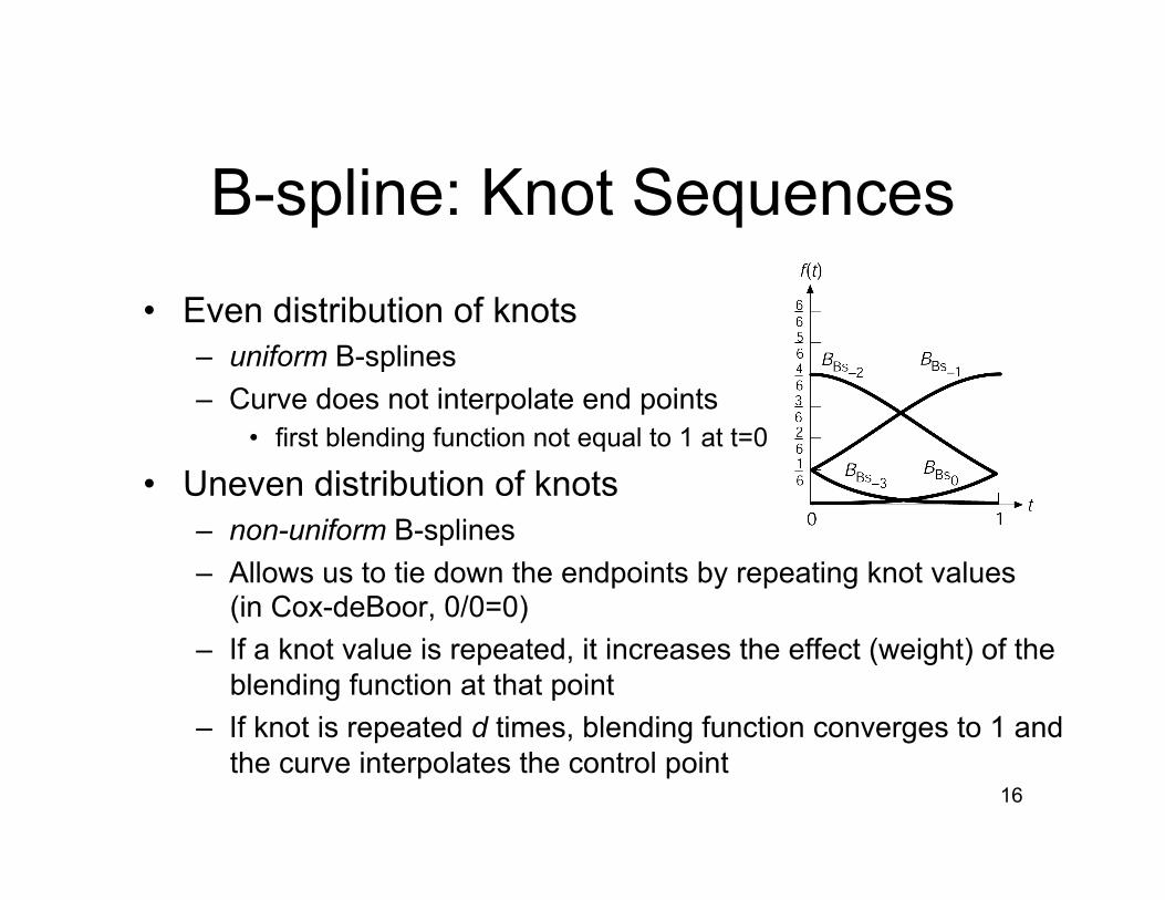
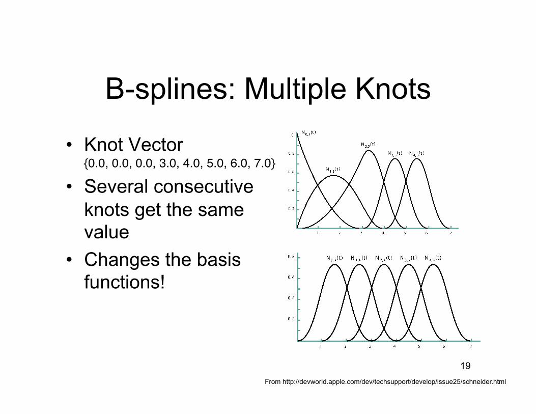
B-spline: Knot Sequences •  Even distribution of knots

–  uniform B-splines –  Curve does not interpolate end points

•  first blending function not equal to 1 at t=0

•  Uneven distribution of knots –  non-uniform B-splines –  Allows us to tie down the endpoints by repeating knot values

(in Cox-deBoor, 0/0=0) –  If a knot value is repeated, it increases the effect (weight) of the

blending function at that point –  If knot is repeated d times, blending function converges to 1 and

the curve interpolates the control point

17

€

Bi,d (t)

)()()(

otherwise,0if,1

)(

1,111

11,,

10,

tBtttttB

tttttB

ttttB

dkkdk

dkdk

kdk

kdk

kkk

−++++

++−

+

+

−

−+

−

−=

<≤

=

B-splines: Cox-deBoor Recursion

•  Cox-deBoor Algorithm: defines the blending functions for spline curves (not limited to deg 3) –  curves are weighted avgs of lower degree curves

•  Let denote the i-th blending function for a B-spline of degree d, then:

18

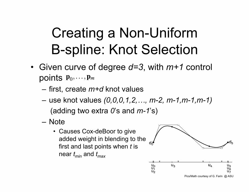
Creating a Non-Uniform B-spline: Knot Selection

•  Given curve of degree d=3, with m+1 control points –  first, create m+d knot values –  use knot values (0,0,0,1,2,…, m-2, m-1,m-1,m-1) (adding two extra 0’s and m-1’s) –  Note

•  Causes Cox-deBoor to give added weight in blending to the first and last points when t is near tmin and tmax

Pics/Math courtesy of G. Farin @ ASU

19

B-splines: Multiple Knots

•  Knot Vector {0.0, 0.0, 0.0, 3.0, 4.0, 5.0, 6.0, 7.0}

•  Several consecutive knots get the same value

•  Changes the basis functions!

From http://devworld.apple.com/dev/techsupport/develop/issue25/schneider.html

20

B-spline Summary ∑=

=m

iidi ptBtp

0, )()(

)()()(

otherwise,0if,1

)(

1,111

11,,

10,

tBtttttB

tttttB

ttttB

dkkdk

dkdk

kdk

kdk

kkk

−++++

++−

+

+

−

−+

−

−=

<≤

=

21

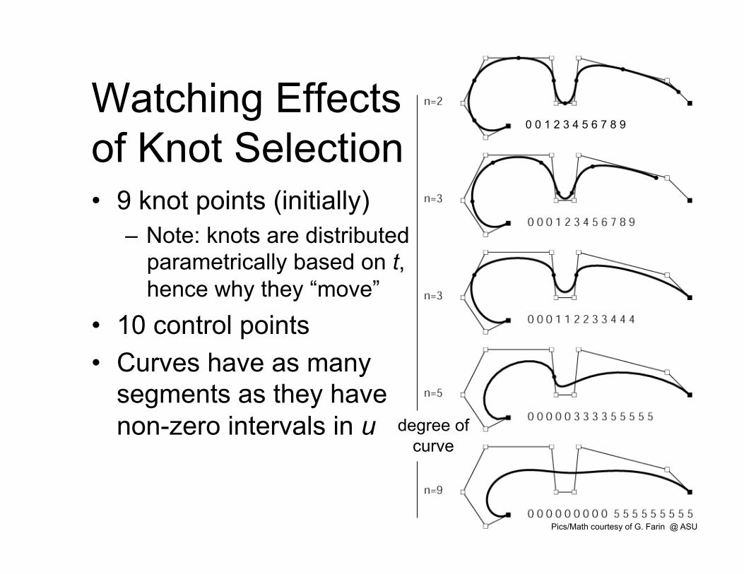
Watching Effects of Knot Selection •  9 knot points (initially)

–  Note: knots are distributed parametrically based on t, hence why they “move”

•  10 control points •  Curves have as many

segments as they have non-zero intervals in u

Pics/Math courtesy of G. Farin @ ASU

degree of curve

0 0 1 2 3 4 5 6 7 8 9

22

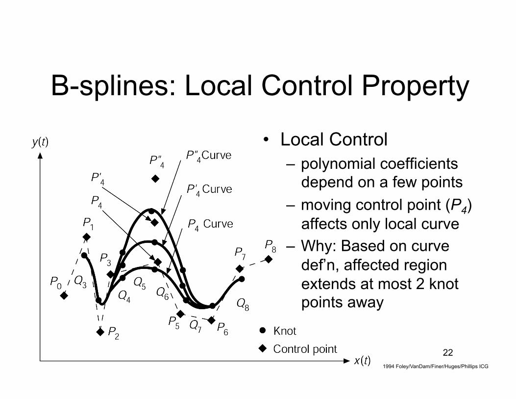
B-splines: Local Control Property

•  Local Control –  polynomial coefficients

depend on a few points –  moving control point (P4)

affects only local curve –  Why: Based on curve

def’n, affected region extends at most 2 knot points away

1994 Foley/VanDam/Finer/Huges/Phillips ICG

23

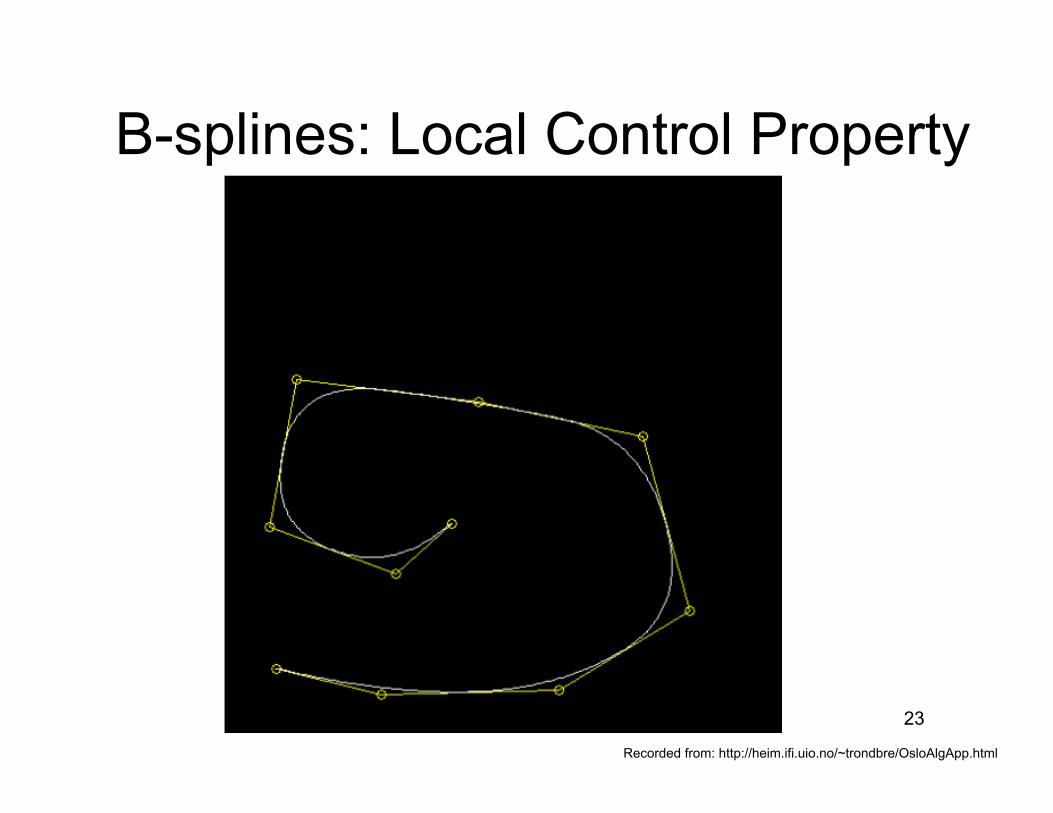
B-splines: Local Control Property

Recorded from: http://heim.ifi.uio.no/~trondbre/OsloAlgApp.html

25

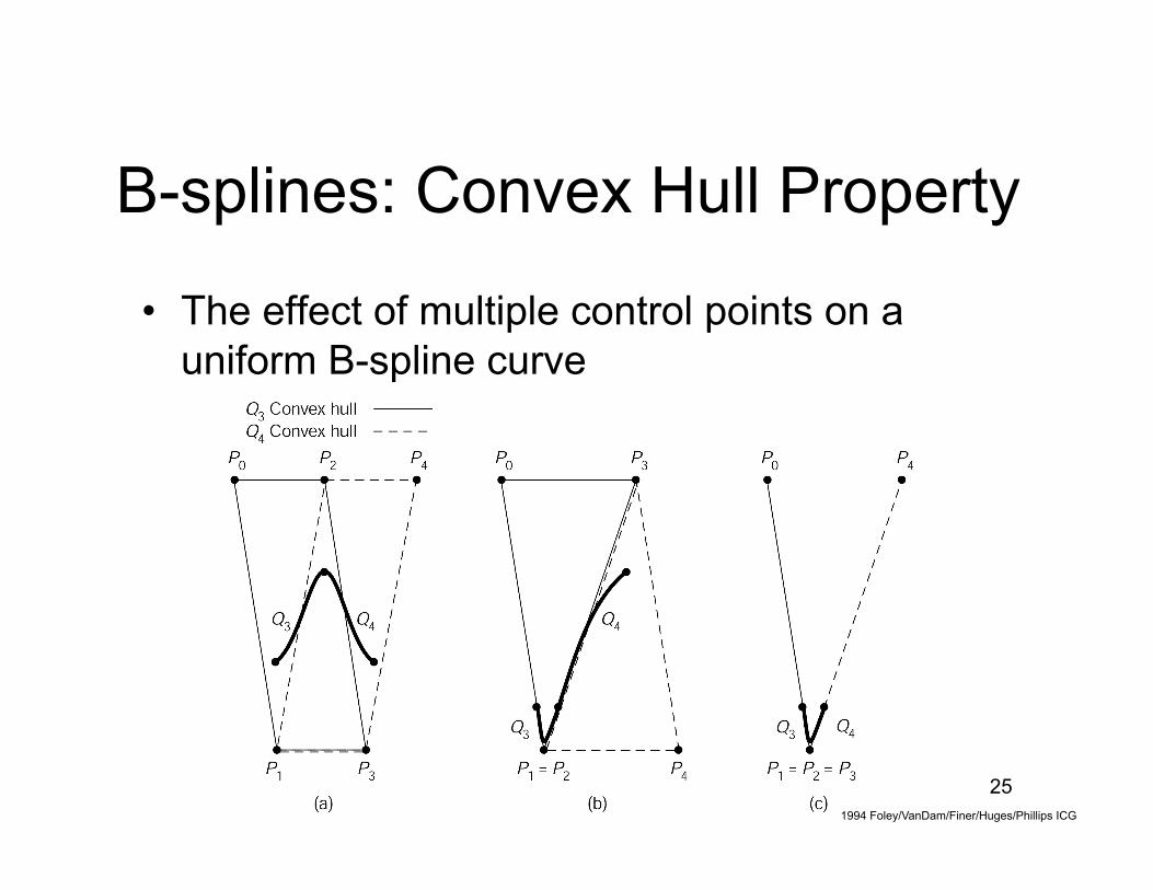
B-splines: Convex Hull Property

•  The effect of multiple control points on a uniform B-spline curve

1994 Foley/VanDam/Finer/Huges/Phillips ICG

26

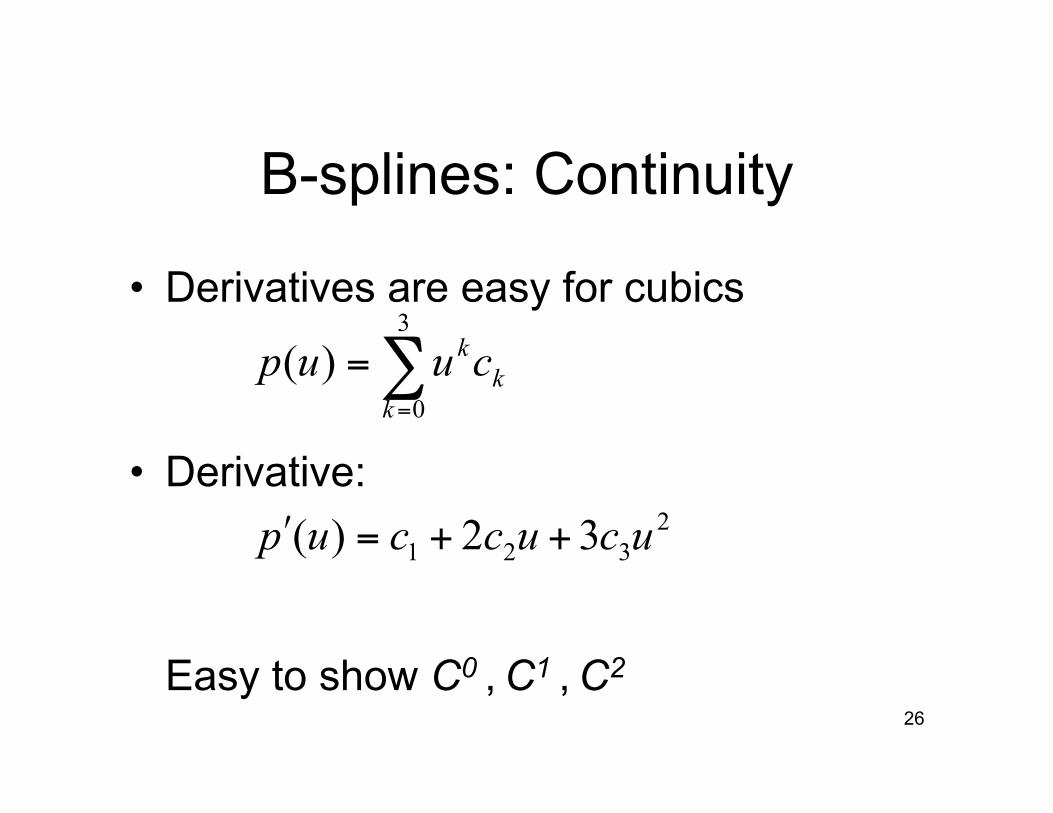
B-splines: Continuity

•  Derivatives are easy for cubics

•  Derivative:

Easy to show C0 , C1 , C2

∑=

=3

0)(

kk

kcuup

2321 32)( ucuccup ++=′

27

B-splines: Setting the Options

•  How to space the knot points? – Uniform

•  equal spacing of knots along the curve – Non-Uniform

•  Which type of parametric function? – Rational

•  x(t), y(t), z(t) defined as ratio of cubic polynomials

– Non-Rational

28

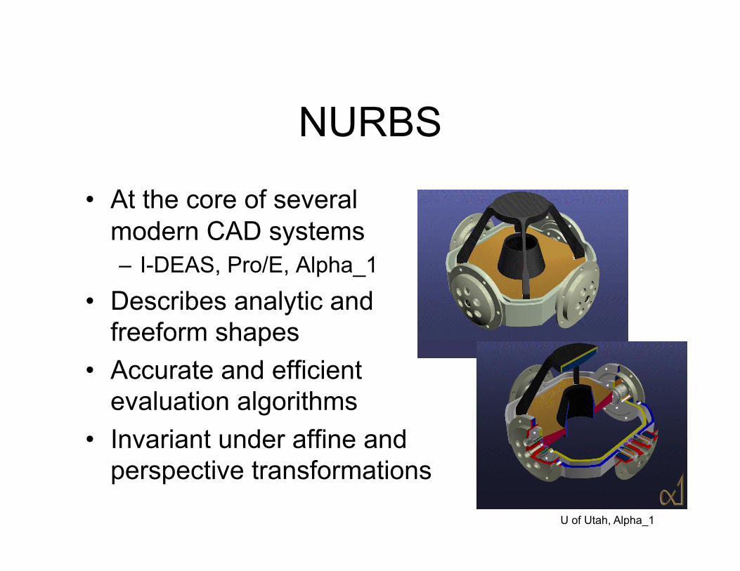
NURBS

•  At the core of several modern CAD systems –  I-DEAS, Pro/E, Alpha_1

•  Describes analytic and freeform shapes

•  Accurate and efficient evaluation algorithms

•  Invariant under affine and perspective transformations

U of Utah, Alpha_1

29

Benefits of Rational Spline Curves

•  Invariant under rotation, scale, translation, perspective transformations –  transform just the control points,

then regenerate the curve –  (non-rationals only invariant under rotation, scale

and translation) •  Can precisely define the conic sections and

other analytic functions –  conics require quadratic polynomials –  conics only approximate with non-rationals

30

NURBS

Non-uniform Rational B-splines: NURBS

•  Basic idea: four dimensional non-uniform B-splines, followed by normalization via homogeneous coordinates –  If Pi is [x, y, z, 1], results are invariant wrt perspective projection

•  Also, recall in Cox-deBoor, knot spacing is arbitrary –  knots are close together,

influence of some control points increases –  Duplicate knots can cause points to interpolate –  e.g. Knots = {0, 0, 0, 0, 1, 1, 1, 1} create a Bézier curve

31

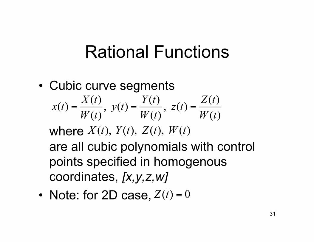
Rational Functions

•  Cubic curve segments

where are all cubic polynomials with control points specified in homogenous coordinates, [x,y,z,w]

•  Note: for 2D case,

)()()( ,

)()()( ,

)()()(

tWtZtz

tWtYty

tWtXtx ===

)( ),( ),( ),( tWtZtYtX

0)( =tZ

32

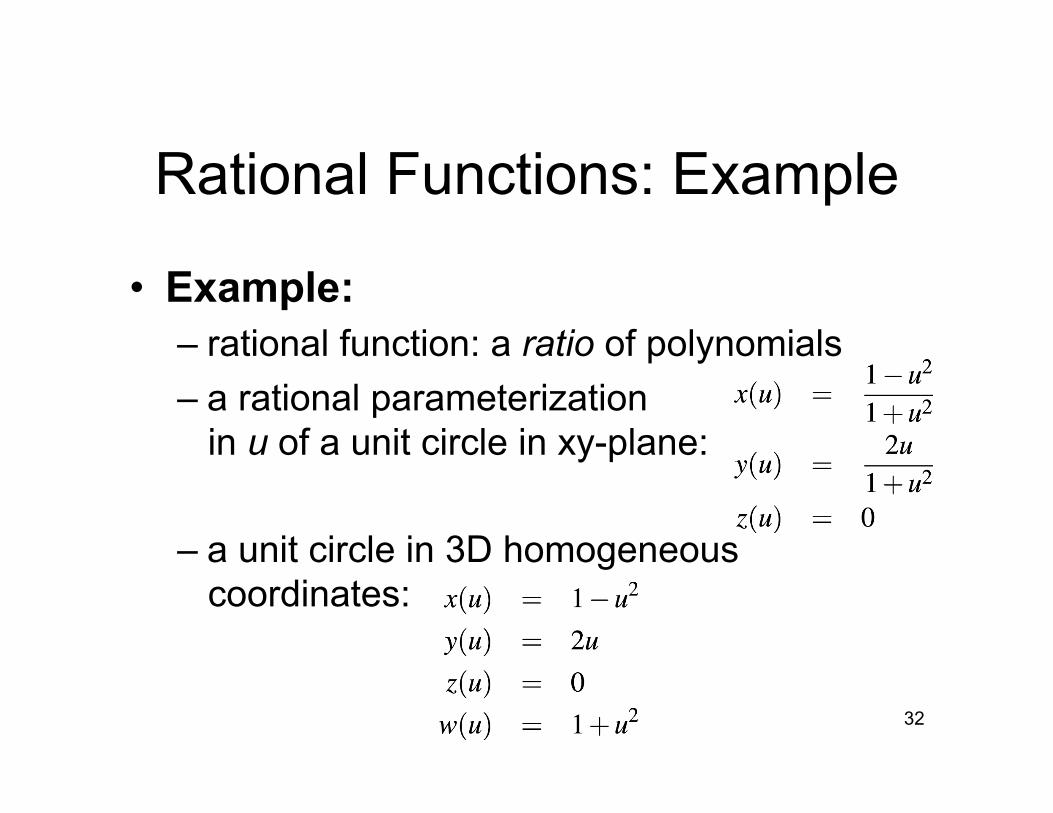
Rational Functions: Example

•  Example: –  rational function: a ratio of polynomials – a rational parameterization

in u of a unit circle in xy-plane:

– a unit circle in 3D homogeneous coordinates:

33

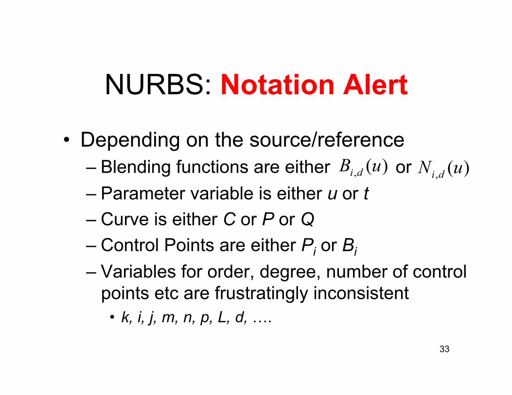
NURBS: Notation Alert

•  Depending on the source/reference – Blending functions are either or – Parameter variable is either u or t – Curve is either C or P or Q – Control Points are either Pi or Bi – Variables for order, degree, number of control

points etc are frustratingly inconsistent •  k, i, j, m, n, p, L, d, ….

)(, uB di )(, uN di

34

NURBS: Notation Alert

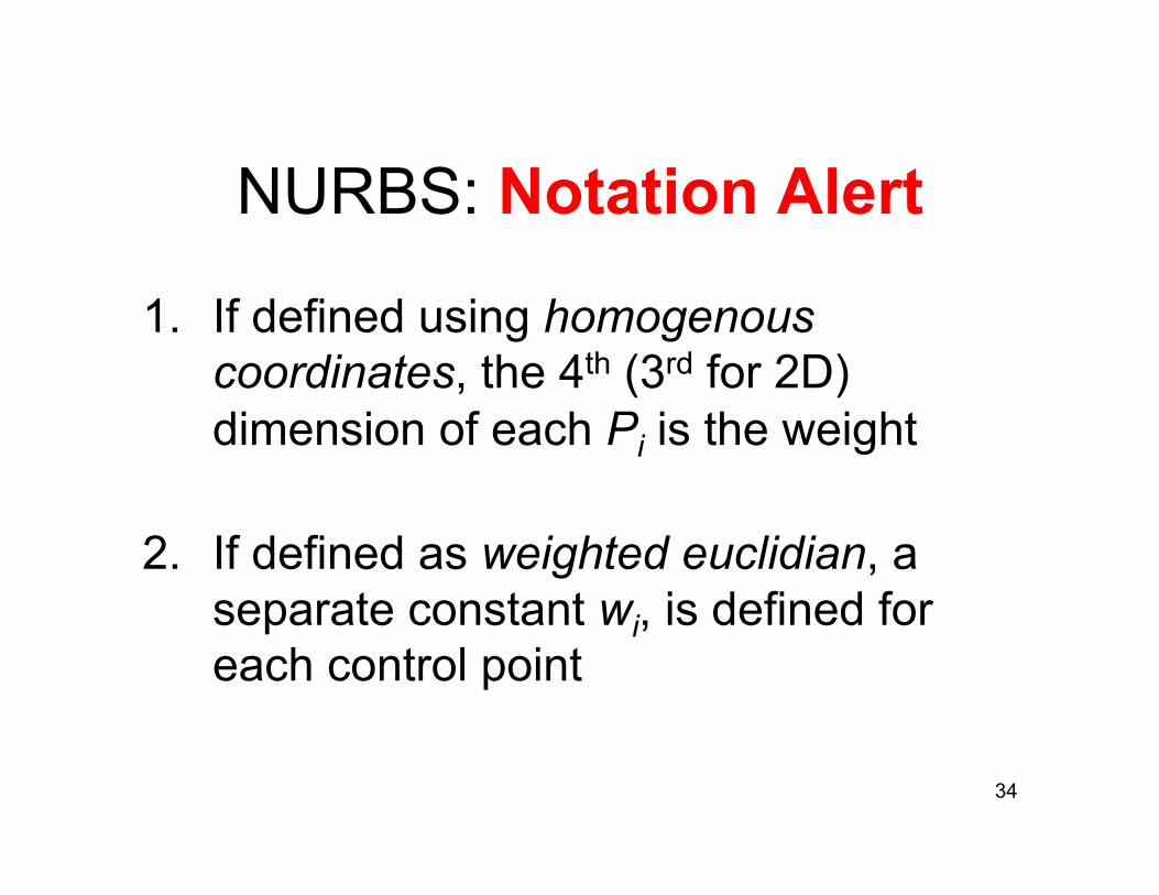
1.  If defined using homogenous coordinates, the 4th (3rd for 2D) dimension of each Pi is the weight

2.  If defined as weighted euclidian, a separate constant wi, is defined for each control point

35

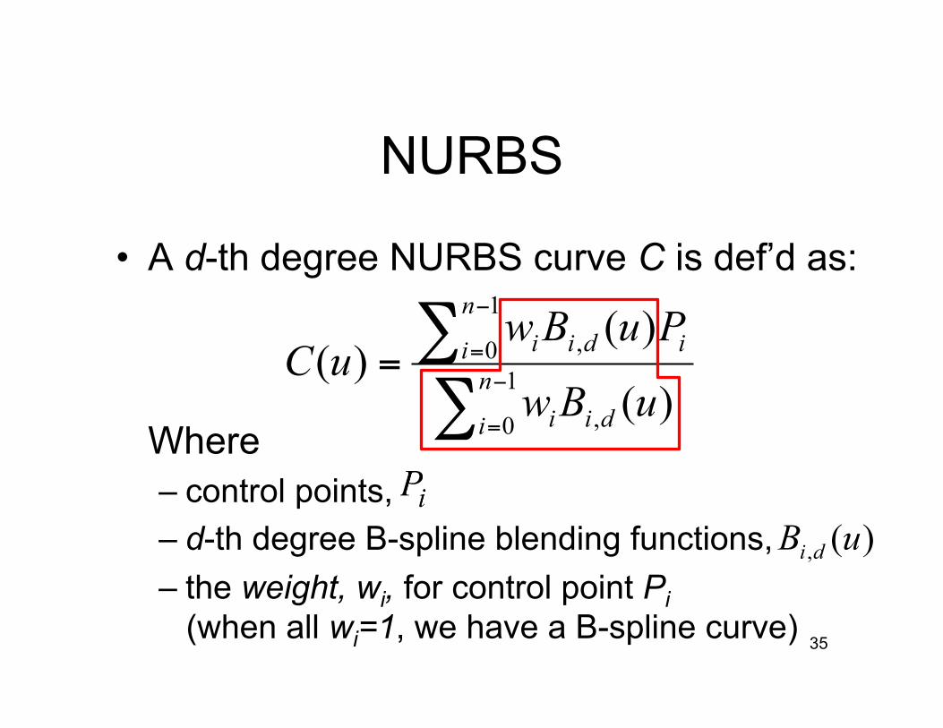
NURBS

•  A d-th degree NURBS curve C is def’d as:

Where – control points, – d-th degree B-spline blending functions, –  the weight, wi, for control point Pi

(when all wi=1, we have a B-spline curve)

∑∑

−

=

−

== 1

0 ,

1

0 ,

)(

)()( n

i dii

n

i idii

uBw

PuBwuC

)(, uB di

36

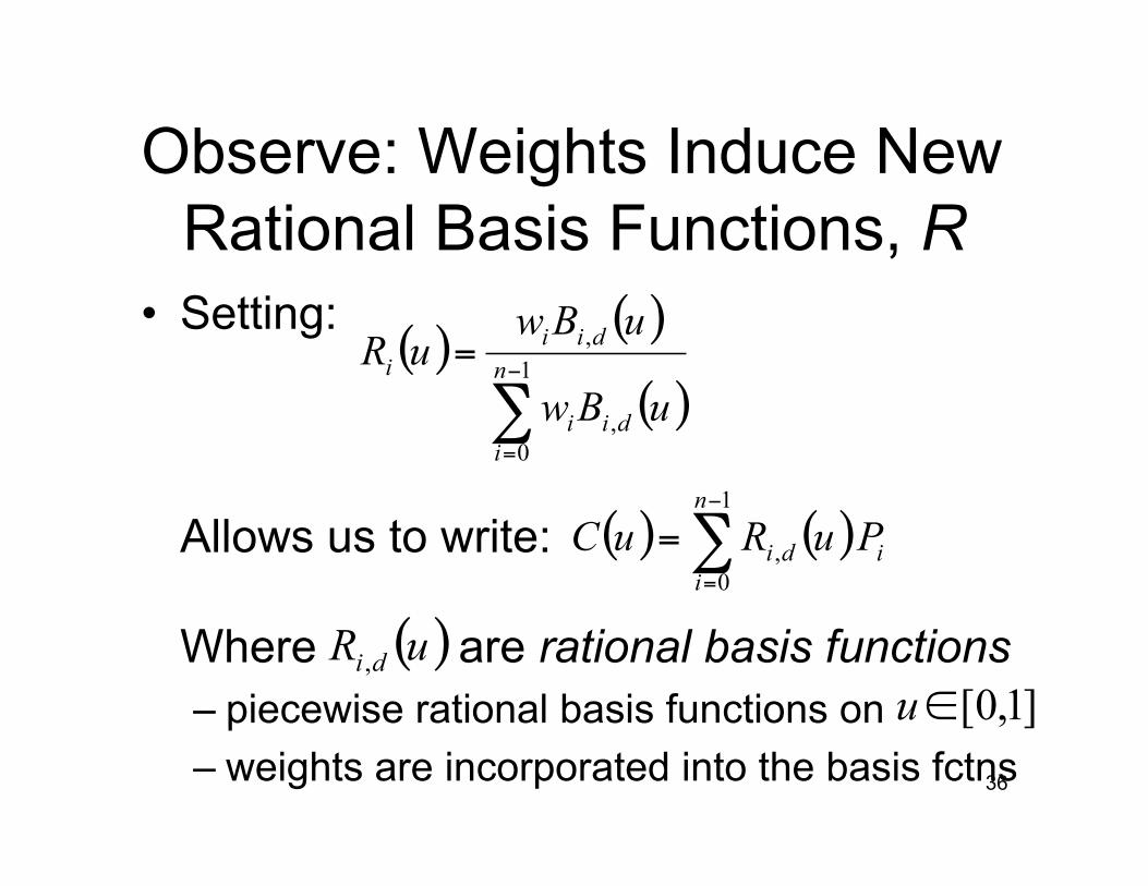
Observe: Weights Induce New Rational Basis Functions, R

•  Setting:

Allows us to write:

Where are rational basis functions – piecewise rational basis functions on – weights are incorporated into the basis fctns

( ) ( )

( )∑−

=

= 1

0,

,n

idii

diii

uBw

uBwuR

( ) ( )∑−

=

=1

0,

n

iidi PuRuC

( )uR di,

]1,0[∈u

37

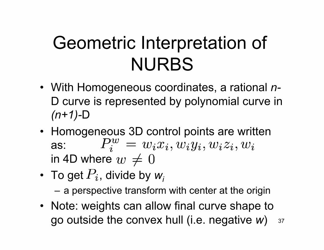
Geometric Interpretation of NURBS

•  With Homogeneous coordinates, a rational n-D curve is represented by polynomial curve in (n+1)-D

•  Homogeneous 3D control points are written as: in 4D where

•  To get , divide by wi –  a perspective transform with center at the origin

•  Note: weights can allow final curve shape to go outside the convex hull (i.e. negative w)

38

NURBS: Examples

{0.0, 1.0, 2.0, 3.0, 4.0, 5.0, 6.0, 7.0} {0.0, 1.0, 2.0, 3.75, 4.0, 4.25, 6.0, 7.0}

•  Unif. Knot Vector •  Non-Unif. Knot Vector

From http://devworld.apple.com/dev/techsupport/develop/issue25/schneider.html

39

NURBS: Examples

•  Knot Vector {0.0, 0.0, 0.0, 3.0, 4.0, 5.0, 6.0, 7.0}

•  Several consecutive knots get the same value

•  Bunches up the curve and forces it to interpolate

From http://devworld.apple.com/dev/techsupport/develop/issue25/schneider.html

40

NURBS: Examples

•  Knot Vector {0.0, 1.0, 2.0, 3.0, 3.0, 5.0, 6.0, 7.0}

•  Several consecutive knots get the same value

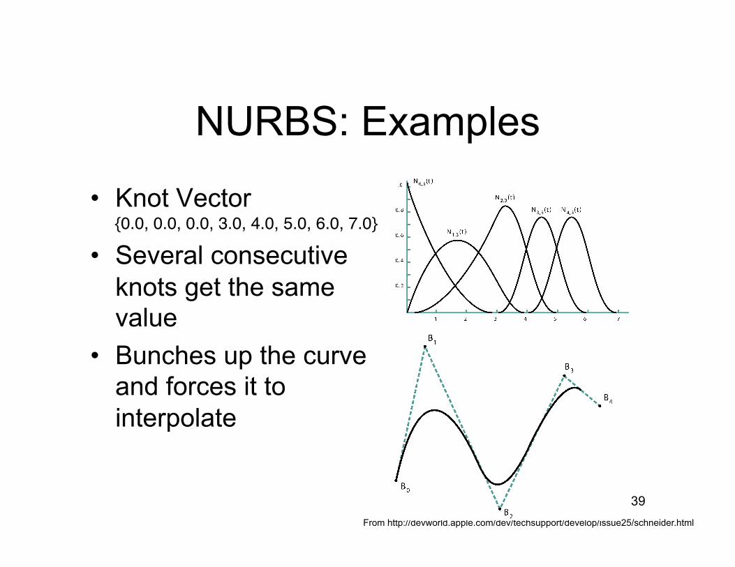
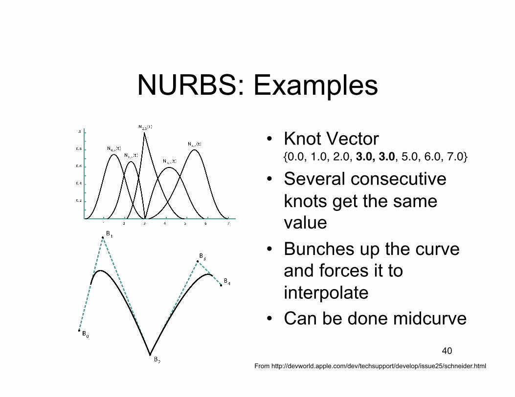
•  Bunches up the curve and forces it to interpolate

•  Can be done midcurve

From http://devworld.apple.com/dev/techsupport/develop/issue25/schneider.html

41

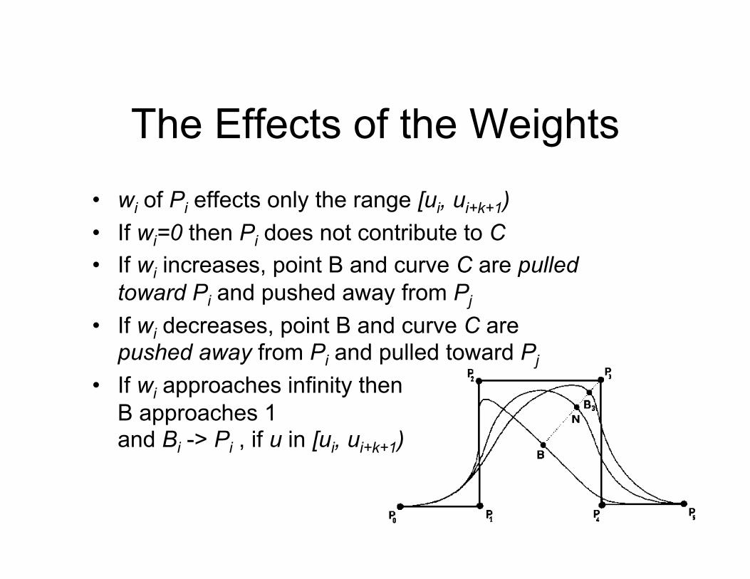
The Effects of the Weights •  wi of Pi effects only the range [ui, ui+k+1) •  If wi=0 then Pi does not contribute to C •  If wi increases, point B and curve C are pulled

toward Pi and pushed away from Pj •  If wi decreases, point B and curve C are

pushed away from Pi and pulled toward Pj •  If wi approaches infinity then

B approaches 1 and Bi -> Pi , if u in [ui, ui+k+1)

42

The Effects of the Weights

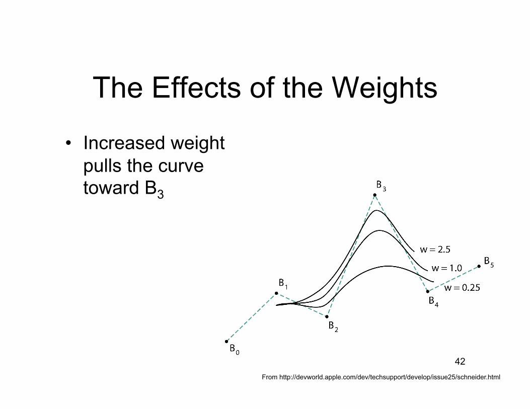
•  Increased weight pulls the curve toward B3

From http://devworld.apple.com/dev/techsupport/develop/issue25/schneider.html

43

Programming assignment 3

•  Input PostScript-like file containing polygons •  Output B/W XPM •  Implement viewports •  Use Sutherland-Hodgman intersection for

polygon clipping •  Implement scanline polygon filling. (You

cannot use flood filling)