prediction of design wind speeds and structural safety
2.1 InTroducTIon and HIsTorIcal background
The establishment of appropriate design wind speeds is a critical first step towards the calculation of design wind loads for structures. It is also usually the most uncertain part of the design process for wind loads, and requires the statistical analysis of historical data on recorded wind speeds.
In the 1930s, the use of the symmetrical bell-shaped Gaussian distribution (Appendix C3.1) to represent extreme wind speeds, for the prediction of long-term design wind speeds, was proposed. However, this failed to take note of the earlier theoretical work of Fisher and Tippett (1928), establishing limiting forms of the distribution of the largest (or smallest) value in a fixed sample, depending on the form of the tail of the parent distribution. The identification of the three types of extreme value distribution was of prime significance to the development of probabilistic approaches in engineering in general.
The use of extreme value analysis for design wind speeds lagged behind the applica-tion to flood analysis. Gumbel (1954) strongly promoted the use of the simpler Type I Extreme Value Distribution for such analyses. However, von Mises (1936) showed that the three asymptotic distributions of Fisher and Tippett could be represented as a single Generalised Extreme Value (GEV) Distribution – this is discussed in detail in the follow-ing section. In the 1950s and the early 1960s, several countries had applied extreme value analyses to predict design wind speeds. In the main, the Type I (by now also known as the ‘Gumbel Distribution’) was used for these analyses. The concept of return period also arose at this time.
The use of probability and statistics as the basis for the modern approach to wind loads was, to a large extent, a result of the work of A.G. Davenport in the 1960s, recorded in several papers (e.g. Davenport, 1961).
In the 1970s and 1980s, the enthusiasm for the then standard ‘Gumbel analysis’ was tempered by events such as Cyclone ‘Tracy’ in Darwin, Australia (1974), and severe gales in Europe (1987), when the previous design wind speeds determined by a Gumbel fitting procedure, were exceeded considerably. This highlighted the importance of
• Sampling errors inherent in the recorded data base, usually <50 years• The separation of data originating from different storm types
The need to separate the recorded data by the storm type was recognised in the 1970s by Gomes and Vickery (1977a).
The development of probabilistic methods in structural design generally, developed in par-allel with their use in wind engineering, followed the pioneering work by Freudenthal (1947, 1956) and Pugsley (1966). This area of research and development is known as ‘structural
reliability’ theory. Limit states design, which is based on probabilistic concepts, was steadily introduced into the design practice from the 1970s onwards.
This chapter discusses modern approaches to the use of extreme value analysis for the prediction of extreme wind speeds for the design of structures. Related aspects of structural design and safety are discussed in Section 2.6.
2.2 prIncIples oF exTreMe Value analysIs
The theory of extreme value analysis of wind speeds, or other geophysical variables, such as flood heights, or earthquake accelerations, is based on the application of one or more of the three asymptotic extreme value distributions identified by Fisher and Tippett (1928), and discussed in the following section. They are asymptotic in the sense that they are the cor-rect distributions for the largest of an infinite population of independent random variables of a known probability distribution. In practice, of course, there will be a finite number in a population, but in order to make predictions, the asymptotic extreme value distributions are still used as empirical fits to the extreme data. Which one of the three is theoretically ‘correct’ depends on the form of the tail of the underlying parent distribution. However, unfortunately, this form is not usually known with certainty due to lack of data. Physical reasoning has sometimes been used to justify the use of one or other of the asymptotic extreme value distributions.
Gumbel (1954, 1958) has covered the theory of extremes in detail. A useful review of the various methodologies available for the prediction of extreme wind speeds, including those discussed in this chapter, has been given by Palutikof et al. (1999).
2.2.1 The geV distribution
The GEV Distribution introduced by von Mises (1936), and later re-discovered by Jenkinson (1955), combines the three extreme value distributions into a single mathematical form:
FU(U) = exp {−[1 − k (U – u)/a]1/k} (2.1)
where FU(U) is the cumulative probability distribution function (see Appendix C) of the maximum wind speed in a defined period (e.g. 1 year).
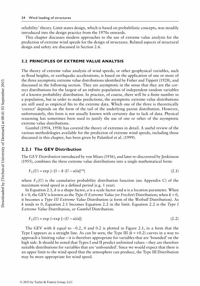
In Equation 2.1, k is a shape factor, a is a scale factor and u is a location parameter. When k < 0, the GEV is known as the Type II Extreme Value (or Frechet) Distribution; when k > 0, it becomes a Type III Extreme Value Distribution (a form of the Weibull Distribution). As k tends to 0, Equation 2.1 becomes Equation 2.2 in the limit. Equation 2.2 is the Type I Extreme Value Distribution, or Gumbel Distribution.
FU(U) = exp {–exp [–(U – u)/a]} (2.2)
The GEV with k equal to −0.2, 0 and 0.2 is plotted in Figure 2.1, in a form that the Type I appears as a straight line. As can be seen, the Type III (k = +0.2) curves in a way to approach a limiting value – it is therefore appropriate for variables that are ‘bounded’ on the high side. It should be noted that Types I and II predict unlimited values – they are therefore suitable distributions for variables that are ‘unbounded’. Since we would expect that there is an upper limit to the wind speed that the atmosphere can produce, the Type III Distribution may be more appropriate for wind speed.
Prediction of design wind speeds and structural safety 35
A method of fitting the GEV Distribution to wind data is discussed in Section 2.4. An alternative method is the method of probability-weighted moments described by Hosking et al. (1985).
2.2.2 return period
At this point, it is appropriate to introduce the term return period, R. It is simply the inverse of the complementary cumulative distribution of the extremes.
i.e. Return period
obability of exceedence1
1 ( ),
PrR
F UU= = −
1
Thus, if the annual maximum is being considered, then the return period is measured in years. Thus, a 50-year return period wind speed has a probability of exceedence of 0.02 (1/50) in any 1 year. It should not be interpreted as recurring regularly every 50 years. The probability of a wind speed, of a given return period, being exceeded in the lifetime of a structure is discussed in Section 2.6.3.
2.2.3 separation by storm type
In Chapter 1, the various types of wind storm that are capable of generating winds strong enough to be important for the structural design were discussed. These different event types will have different probability distributions, and therefore should be statistically analysed separately; however, this is usually quite a difficult task as weather bureaus or meteorological offices do not normally record the necessary information. If anemograph records such as those shown in Figures 1.5 and 1.7 are available for older data, these can be used for identification purposes! Modern automatic weather stations (AWS) can generate wind speed and direction data at short intervals of as low as 1 min. These can be used to reconstruct time histories similar to those in Figures 1.5 and 1.7, and assist in identifying storm types.
Reduced variate: –In[–In(FU)]–6–4–2–2 –1–3
00 1 2 3 4
2468
Type I k = 0Type III k = +0.2Type II k = –0.2
(U – u)/a
Figure 2.1 The GEV Distribution (k = −0.2, 0, +0.2).
The relationship between the combined return period, Rc, for a given extreme wind speed due to winds of either type, and for those calculated separately for storm types 1 and 2, (R1 and R2) is
1
11
11
1
1 2−
= −
−
R R Rc
(2.3)
Equation 2.3 relies on the assumption that exceedences of wind speeds from the two dif-ferent storm types are independent events.
2.2.4 simulation methods for tropical cyclone wind speeds
The winds produced by severe tropical cyclones, also known as ‘hurricanes’ and ‘typhoons’, are the most severe on Earth (apart from those produced by tornadoes which affect very small areas). However, their infrequent occurrence at particular locations often makes the historical record of recorded wind speeds an unreliable predictor for design wind speeds. An alternative approach, which gained popularity in the 1970s and early 1980s, was the simulation or ‘Monte-Carlo’ approach, introduced originally for offshore engineering by Russell (1971). In this procedure, satellite and other information on storm size, intensity and tracks are made use of to enable a computer-based simulation of wind speed (and in some cases direction) at particular sites. Usually, established probability distributions are used for parameters such as central pressure and radius to maximum winds. A recent use of these models is for damage prediction for insurance companies. The disadvantage of this approach is the subjective aspect resulting from the complexity of the problem. Significantly varying predictions could be obtained by adopting different assumptions. Clearly, whatever recorded data that are available should be used to calibrate these models.
2.2.5 compositing data from several stations
No matter what type of probability distribution is used to fit historical extreme wind series, or what fitting method is used, extrapolations to high return periods for ultimate limit states design (either explicitly, or implicitly through the application of a wind load factor) are usually subject to significant sampling errors. This results from the limited record lengths usually available to the analyst. In attempts to reduce the sampling errors, a recent practice has been to combine records from several stations with perceived similar wind climates to increase the available records for extreme value analysis. Thus, ‘superstations’ with long records can be generated in this way.
For example, in Australia, stations in a huge region in the southern part of the country have been judged to have similar statistical behaviour, at least as far as the all-direction extreme wind speeds are concerned. A single set of design wind speeds has been specified for this region (Standards Australia, 1989, 2011; Holmes, 2002). A similar approach has been adopted in the United States (ASCE, 1998, 2010; Peterka and Shahid, 1998).
2.2.6 correction for gust duration
Wind data are recorded and supplied by meteorological offices, or bureaus, after being averaged over certain time intervals. The most common averaging time is 10 min. Gust data obtained by modern AWS are typically averaged over 3 s. However, earlier data obtained from older anemometers and analogue-recording systems are usually of a shorter duration
Prediction of design wind speeds and structural safety 37
(e.g. Miller et al., 2013). A time series of gust data may need to be corrected to a common gust duration (see Section 3.3.3), before extreme value analysis is carried out. Correction factors can be derived using random process theory, with some assumptions on the form of the spectral density of the turbulence (Section 3.3.4), as a function of mean wind speed and turbulence intensity (e.g. Holmes and Ginger, 2012).
2.2.7 Wind direction effects and wind direction multipliers
Increased knowledge of the aerodynamics of buildings and other structures, through wind-tunnel and full-scale studies, has revealed the variation of structural response as a function of wind direction as well as speed. The approaches to probabilistic assessment of wind loads including direction can be divided into those based on the parent distribution of wind speed, and those based on extreme wind speeds. In many countries, the extreme winds are produced by rare severe storms such as thunderstorms and tropical cyclones, and there is no direct rela-tionship between the parent population of regular everyday winds, and the extreme winds. For such locations (which would include most tropical and sub-tropical countries), the latter approach may be more appropriate. Where a separate analysis of extreme wind speeds by a direction sector has been carried out, the relationship between the return period, Ra, for exceedence of a specified wind speed from all-direction sectors, and the return periods for the same wind speed from direction sectors θ1, θ2 and so on is given in Equation 2.4.
1
11
1
1
−
= −
=
∏R Ra i
N
iθ (2.4)
Equation 2.4 follows from an assumption that the wind speeds from each direction sector are statistically independent of each other, and is a statement of the following:
Probability that a wind speed U is not exceeded for all wind directions = (probability that U is not exceeded from direction 1)×(probability that U is not exceeded from direction 2)×(probability that U is not exceeded from direction 3)… and so on
Equation 2.4 is a similar relationship to Equation 2.3 for combining extreme wind speeds from different types of storms. A similar approach can be adopted for combining the extreme wind pressure, or a structural response, from contributions from different directions (e.g. Holmes, 1990, Section 9.11).
The use of Equation 2.4, or other full probabilistic methods of treating the directional effects of wind, adds a considerable degree of complexity when applied to the structural design for wind. To avoid this, simplified methods of deriving direction multipliers, or direc-tional factors, have been developed (e.g. Cook, 1983; Melbourne, 1984; Cook and Miller, 1999). These factors, which have been incorporated into some codes and standards, allow climatic effects on wind direction to be incorporated into wind load calculations in an approximate way. Generally, the maximum (or minimum) value of a response variable, from any direction sector, is used for design purposes.
Three methods that have been suggested for deriving directional wind speeds, or direction multipliers, are:
a. The extreme wind speeds, given a direction sector, are fitted with an extreme value probability distribution, in the same way as the all-direction winds. Then direction
multipliers are obtained by dividing the wind speed with a specified exceedence prob-ability by the all-direction wind speed with the same exceedence probability. This is an unconservative approach when applied to structural response, as it ignores contribu-tions to the combined probability of response from more than one direction sector.
b. The extreme wind speeds within a direction sector are fitted with an extreme value probability distribution in the same way as the all-direction winds. The target prob-ability of exceedence of the all-direction wind is then divided by the number of direc-tion sectors. The wind speed within each direction sector is then calculated for the reduced exceedence probability. These wind speeds are then divided by the all-direc-tion wind speed with the original target probability to give wind direction multipliers. This approach (proposed by Cook, 1983) clearly gives higher direction multipliers than Method (a), and is generally regarded as being a conservative one, when applied to codes and standards for the design of buildings.
c. As an empirical approach between the unconservative Method Approach (a) and the conservative Method (b), Melbourne (1984) suggested what amounts to a modifica-tion to Method (a), to render it less unconservative, by specifying a probability of exceedence for the directional winds of the target probability of the all-direction wind speeds, divided by one-quarter of the number of direction sectors. In effect, Melbourne (1984) suggested that only two sectors from eight sectors in Equation 2.4, when N = 8, are effective, on average, in contributing to the combined probability of a structural response – that is a 90° sector from the total of 360°. Wind direction multipliers are then obtained by dividing the all-direction wind speed with the target probability of exceedence, as for Methods (a) and (b).
Kasperski (2007) derived direction wind speeds and multipliers, Md, for Dusseldorf, Germany, using Methods (a) and (b). These values are shown in Table 2.1.
For this location, the southwesterly and westerly sectors (i.e. 210–270°) are the dominant ones for strong winds, due to the effect of Atlantic gales. It will be noted that Method (a) gives values of Md that are all <1.0. The conservative nature of Method (b) is shown by the values of 1.02 for wind directions from 210° to 270°.
Table 2.1 Direction multipliers for Dusseldorf, Germany
Prediction of design wind speeds and structural safety 39
Method (c), representing an empirical compromise between Methods (a) and (b), generally gives maximum values of Md close to 1.0. This approach has been used to derive wind direc-tion multipliers for Australia and New Zealand in the Standard AS/NZS 1170.2 (Standards Australia, 2011).
Besides the use of wind direction multipliers, or the direct application of Equation 2.4, there are several other methods of treating the varying effects of wind direction on the response of buildings. Several of these are discussed in Section 9.11.
2.3 exTreMe WInd esTIMaTIon by THe Type I dIsTrIbuTIon
2.3.1 gumbel’s method
Gumbel (1954) gave an easily usable methodology for fitting recorded annual maxima to the Type I Extreme Value Distribution. This distribution is a special case of the GEV Distribution discussed in Section 2.2.1. The Type I Distribution takes the form of Equation 2.2 for the cumulative distribution FU(U):
FU(U) = exp {–exp [–(U – u)/a]}
where u is the mode of the distribution, and a is a scale factor.The return period, R, is directly related to the cumulative probability distribution, FU(U),
of the annual maximum wind speed at a site as follows:
R
F UU= −
11 ( )
(2.5)
Substituting for FU(U) from Equation 2.5 in Equation 2.2, we obtain:
U u a
RR e e= + − − −
log log 1
1
(2.6)
For large values of return period, R, Equation 2.6 can be written as
U u a RR e≅ + log (2.7)
In Gumbel’s original extreme value analysis method (applied to flood prediction as well as extreme wind speeds), the following procedure is adopted:
• The largest wind speed in each calendar year of the record is extracted.• The series is ranked in order of smallest to largest: 1,2,…m…. to N.• Each value is assigned a probability of non-exceedence, p, according to
• y is an estimate of the term in {} brackets in Equation 2.6.• The wind speed, U, is plotted against y, and a line of ‘best fit’ is drawn, usually by
means of linear regression.
As may be seen from Equation 2.7 and Figure 2.1, the Type I or Gumbel Distribution will predict unlimited values of UR, as the return period, R, increases. That is as R becomes larger, UR as predicted by Equation 2.6 or 2.7 will also increase without limit. As discussed in Section 2.2.1, this is not consistent with the physical argument that there are upper limits to the wind speeds that can be generated in the atmosphere in different types of storms.
2.3.2 gringorten’s method
The Gumbel procedure, as described in Section 2.3.1, has been used many times to analyse extreme wind speeds for many parts of the world.
Assuming that the Type I Extreme Value Distribution is in fact the correct one, the fitting method, due to Gumbel, is biased, that is Equation 2.8 gives distorted values for the prob-ability of non-exceedence, especially for high values of p near 1. Several alternative fitting methods have been devised which attempt to remove this bias. However, most of these are more difficult to apply, especially if N is large, and some involve the use of computer pro-grammes to implement. A simple modification to the Gumbel procedure, which gives nearly unbiased estimates for this probability distribution, is due to Gringorten (1963). Equation 2.8 is replaced by the following modified formula:
Fitting of a straight line to U versus the plotting parameter, p, then proceeds as for the Gumbel method.
2.3.3 Method of Moments
The simplest method of fitting the Type I Extreme Value Distribution to a set of data is known as the ‘Method of Moments’. It is based on the following relationships between the mean and standard deviation of the distribution, and the mode and scale factor (or slope).
Mean = u + 0.5772a (2.11)
Standard deviation = π
6
a
(2.12)
The method to estimate the parameters, u and a, of the distribution simply entails the calculation of the sample mean, μ, and standard deviation, σ, from the data, and then esti-mating u and a by the use of the inverse of Equations 2.11 and 2.12, that is
Prediction of design wind speeds and structural safety 41
Once the parameters u and a have been determined, predictions of the extreme wind speed for a specified return period, R, are made using Equation 2.6 or 2.7.
Another procedure is the ‘best linear unbiased estimators’ proposed by Lieblein (1974), in which the annual maxima are ordered, and the parameters of the distribution are obtained by weighted sums of the extreme values.
2.3.4 example of fitting the Type I distribution to annual maxima
Wind gust data have been obtained from a military airfield at East Sale, Victoria, Australia, con-tinuously since late 1951. The anemometer position has been constant throughout that period, and the height of the anemometer head has always been the standard meteorological value of 10 m. Thus, in this case, no corrections for height and terrain are required. Also, the largest gusts have almost entirely been produced by gales from large synoptic depressions (Section 1.3.1). However, the few gusts that were produced by thunderstorm downbursts were elimi-nated from the list, in order to produce a statistically consistent population (see Section 2.2.3).
The annual maxima for the 47 calendar years 1952–1998 are listed in Table 2.2. The values in Table 2.2 are sorted in order of increasing magnitude (Table 2.3) and assigned a probability, p, according to (i) the Gumbel formula (Equation 2.8), and (ii) the Gringorten formula (Equation 2.10). The reduced variate, −loge(−loge p), according to Equation 2.9, is formed for both cases. These are tabulated in Table 2.3. The wind speed is plotted against the reduced variates, and straight lines are fitted by linear regression (‘least squares’ method). The results of this are shown in Figures 2.2 and 2.3, for the Gumbel and Gringorten meth-ods, respectively. The intercept and slope of these lines give the mode, u, and slope, a, of the fitted Type I Extreme Value Distribution, according to Equation 2.1. u and a can also be estimated from the calculated mean and standard deviation (shown in Table 2.1) by the Method of Moments using Equations 2.13 and 2.14.
Predictions of extreme wind speeds for various return periods can then readily be obtained by application of either Equation 2.6 or 2.7. Table 2.4 lists these predictions based on the Gumbel and Gringorten fitting methods, and by the Method of Moments. For return periods up to 500 years, the predicted values by the three methods are within 1 m/s of each other. However, these small differences are swamped by sampling errors, that is the errors inher-ent in trying to make predictions for return periods of 100 years or more from <50 years of data. This problem is illustrated by the following exercise. The problem of high sampling errors can often be circumvented by compositing data, as discussed in Section 2.2.5.
ExERcISE
Re-analyse the annual maximum gust wind speeds for East Sale for the years 1952–1997, that is ignore the high value recorded in 1998. Compare the resulting predictions of design wind speeds for (a) 50-years return period, and (b) 1000-years return period, and comment.
2.3.5 general penultimate distribution
For extreme wind speeds that are derived from a Weibull parent distribution (see Section 2.5), Cook and Harris (2004) have proposed a ‘General penultimate’ Type I, or Gumbel Distribution. This takes the form of Equation 2.15.
FU(U) = exp {–exp [–(Uw – uw)/aw]} (2.15)
where w is the Weibull exponent of the underlying parent distribution (see Equation 2.22).
Comparing Equation 2.15 with Equation 2.2, it can be seen that Equation 2.15 represents a Gumbel Distribution for a transformed variable, Z, equal to Uw.
If the parent wind speed data are available for a site, w can be obtained directly from fitting a Weibull Distribution to that site. Alternatively, the penultimate distribution of Equation 2.15 can be treated as a three-parameter (u, a and w) distribution and fitted directly to the extreme wind data, without knowing the parent distribution directly.
The Weibull exponent, w, is typically in the range of 1.3–2.0; in that case, when Equation 2.15 is plotted in the Gumbel form (Figure 2.2), the resulting line curves downwards, and is similar in shape to the Type III Extreme Value Distribution. The main difference is that the latter has a finite upper limit, whereas for the penultimate distribution, Uw, and hence U, is
Reduced variate (Gumbel)–2 –1 0
01020
304050
East sale gust wind speeds 1952–1998
Win
d sp
eed
(m/s
)
1 2 3 4 5 6 7
y = 2.66x + 27.81
8
Figure 2.2 Analysis of the annual maximum wind gusts from East Sale using the Gumbel method.
Reduced variate (Gringorten)–2 –1 0
0
10
20
30
40
50East sale gust wind speeds 1952–1998
Win
d sp
eed
(m/s
)
1 2 3 4 5 6 7
y = 2.51x + 27.84
8
Figure 2.3 Analysis of East Sale data using the Gringorten fitting method.
Table 2.4 Prediction of extreme wind speeds for East Sale (synoptic winds)
Prediction of design wind speeds and structural safety 45
unlimited. However, for practical design situations, the two distributions give very similar predictions (Holmes and Moriarty, 2001).
2.4 THe peaks-oVer-THresHold approacH
The approach of extracting a single maximum value of wind speed from each year of his-torical data obviously has limitations in that there may be many storms during any year, and only one value from all these storms is being used. A shorter reference period than a year could, of course, be used to increase the amount of data. However, it is important for extreme value analysis that the data values are statistically independent – this will not be the case if a period as short as 1 day is used. An alternative approach which makes use only of the data of relevance to extreme wind prediction is the peaks, or excesses, over threshold approach (e.g. Davison and Smith, 1990; Lechner et al., 1992; Holmes and Moriarty, 1999). The method is also known as the ‘conditional mean exceedence’ (CME) method.
A brief description of the method is given here. This is a method which makes use of all wind speeds from independent storms above a particular minimum threshold wind speed, uo (say 20 m/s). There may be several of these events, or none, during a particular year. The basic procedure is as follows:
• Several threshold levels of wind speed are set: uo, u1, u2 and so on (e.g. 20, 21, 22 …m/s).• The exceedences of the lowest level uo by the maximum storm wind are identified, and
the number of crossings of this level per year, λ, is calculated.• The differences (U − uo) between each storm wind and the threshold level uo are calcu-
lated and averaged (only positive excesses are counted).• The previous step is repeated for each level, u1, u2 and so on, in turn.• The mean excess is plotted against the threshold level.• A scale factor, σ, and a shape factor, k, are determined from the following equations
(Davison and Smith, 1990):
Slope Intercept= −
+σ+=k
k k( ) ( )1 1 (2.16)
Prediction of the R-year return period wind speed, UR, can then be calculated from:
UR = uo + σ[1 − (λR)−k]/k (2.17)
In Equation 2.17, the shape factor, k, is normally found to be positive (usually around 0.1). As R increases to very large values, the upper limit to UR of uo + (σ/k) is gradually approached.
When k is zero, it can be shown mathematically that Equation 2.17 reduces to Equation 2.18.
UR = uo + σ loge(λR) (2.18)
The similarity between Equations 2.7 and 2.18 should be noted.The highest threshold level, un, should be set so that it is exceeded by at least 10 wind
speeds. An example of this method is given in the following section.
2.4.1 example of the use of the ‘peaks over threshold’ method
Daily wind gusts at several stations in the area of Melbourne, Australia, have been recorded since the 1940s. Those at the four airport locations of Essendon, Moorabbin, Melbourne Airport (Tullamarine), and Laverton are the most useful since the anemometers are located at positions most closely matching the ideal open-country conditions, and away from the direct influence of buildings. Table 2.5 summarises the data available from these four stations.
The two most common types of event-producing extreme wind in the Melbourne area are gales produced by the passage of large low pressure or frontal systems (‘synoptic’ winds – see Section 1.3.1), and severe thunderstorm ‘downbursts’ (Section 1.3.3). Downbursts are usually accompanied by thunder, but the occurrence of thunder does not necessarily mean that an extreme gust has been generated by a downburst. The occurrences of downbursts in the data from the four stations were identified by inspection of the charts stored by the Australian Bureau of Meteorology or the National Archives. Table 2.5 shows that the rate of occurrence of downbursts >21 m/s is quite low (around one per year at each station); however, as will be seen, they are significant contributors to the largest gusts.
The largest recorded gusts in the Melbourne area are listed in Table 2.6. Approximately half of these were generated by downbursts.
Extreme value analysis of the data was carried out in the following stages:
• Daily gusts over 21 m/s were retained for analysis.• Gusts generated by downbursts were identified by inspection of anemometer charts,
and separated from the synoptic gusts.• The data from the four stations were composited into single data sets, for both down-
burst and synoptic gusts.• The synoptic data were corrected to a uniform height (10 m), and approach terrain
(open country), using correction factors according to the direction derived from wind-tunnel tests for each station.
• For both data sets, the ‘excesses over threshold’ analysis was used to derive relation-ships between wind speed and return period.
The last stage enabled a scale factor, σ, and a shape factor, k, to be determined in the relationship:
UR = uo + σ[1 − (λR)−k]/k
uo is the lowest threshold – in this case 21 m/s, and λ is average annual rate of exceedence of uo, for the combined data sets. For the current analysis, λ was 23.4 for the synoptic data, and 0.97 for the downburst data.
The results of the two analyses were expressed in the following forms for the Melbourne data:
Prediction of design wind speeds and structural safety 47
For synoptic winds:
U RR = − −68 3 39 3 10 059. . .
(2.19)
For downburst winds:
U RR = − −69 0 48 1 20 108. . .
(2.20)
The combined probability of exceedence of a given gust speed from either type of wind is obtained by substituting in Equation 2.3:
11 1
68 339 3
169 0
48 1
10 059
RU U
C
R R= − − −
− −
..
..
.11
0 108.
(2.21)
Equations 2.19 through 2.21 are plotted in Figure 2.4. The lines corresponding to Equations 2.19 and 2.20 cross at a return period of 30 years. It can also be seen that the combined wind speed return period relationship is asymptotic to the synoptic line at low return periods, and to the downburst line at high return periods.
Table 2.6 Largest recorded gusts in the Melbourne area 1940–1997
Date Station Gust speed (knots) Gust speed (m/s) Type
The peaks-over-threshold approach can be applied to winds separated by a direction sector. This is done in Figure 2.5 which shows a wind speed versus return period for a number of cases using, again, combined gust data, from four stations in the Melbourne area, for syn-optic wind events:
• Gust wind speeds separately analysed for 11 direction sectors of 22.5° width. For the remaining five sectors (ENE to SSE), there was insufficient data for a meaningful analysis to be carried out.
• Combined data from all-direction sectors, analysed as a single data set.• A combined distribution obtained by combining distributions for directional sectors,
according to Equation 2.4.
A peaks-over-threshold approach was used, but in this case, the shape factor, k, was ‘forced’ to be zero, and Equation 2.18 was used for the predictions for the 11 direction sectors and ‘all directions’ data. This effectively resulted in Gumbel Distributions, forming straight lines on the wind speed (linear) versus return period (logarithmic) graphs.
There is good agreement for the ‘all-directions’ line, and the ‘combined directions’ line, indicating the independence of the data from the various direction sectors, and the validity of Equation 2.4.
2.5 parenT WInd dIsTrIbuTIons
For some design applications, it is necessary to have information on the distribution of the complete population of wind speeds at a site. An example is the estimation of fatigue damage for which an account must be taken of damage accumulation over a range of wind storms (see Section 5.6). The population of wind speeds produced by synoptic wind storms at a site is usually fitted with a distribution of the Weibull type:
50
V0.2
s (m
/s)
4540353025201510
50
10 100Return period, R (years)
1000 10,000NNWCombined directions
NWWNW
WSW
SW
SSWSNE
NNE
N
All directionsMelbourne composite 1940–1997 – synoptic winds
W
1
Figure 2.5 Gumbel probability distributions fitted to gust data for direction sectors from the Melbourne area.
Prediction of design wind speeds and structural safety 49
f UwU
cUcU
w
w
w
( ) exp=
−−
1
(2.22)
Equation 2.22 represents the probability density function for mean wind speeds produced by synoptic events. There are two parameters: a scale factor, c, which has units of wind speed, and a shape factor, w, which is dimensionless (see also Appendix C3.4). The prob-ability of exceedence of any given wind speed is given by Equation 2.23
1 − = −
F UUc
w
( ) exp
(2.23)
Typical values of c are 3–10 m/s, and w usually falls in the range 1.3–2.0. An example of a Weibull fit to recorded meteorological data is shown in Figure 2.6.
Several attempts have been made to predict extreme winds from knowledge of the parent distribution of wind speeds, and thus make predictions from quite short records of wind speed at a site (e.g. Gomes and Vickery, 1977b). The ‘asymptotic’ extreme value distribu-tion for a Weibull parent distribution is the Type I, or Gumbel Distribution. However, for extremes drawn from a finite sample (e.g. annual maxima), the ‘penultimate’ Type I, as discussed in Section 2.3.2, is the more appropriate extreme value distribution.
However, it should be noted that both the Weibull Distribution and the Type I Extreme Value Distribution will give unlimited wind speeds with reducing probability of exceedence.
2.6 WInd loads and sTrucTural saFeTy
The development of structural reliability concepts – that is the application of probabilistic methods to the structural design process – has accelerated the adoption of probabilistic
1.0
Data
Loxton 1984–2000 (all directions)
Weibull fit (k = 1.36, c = 3.40)
0.8
0.6
0.4
0.2
0.00 5 10 15
Wind speed (m/s)20 25
Figure 2.6 Example of a Weibull Distribution fit to the parent population of synoptic winds.
methods into wind engineering since the 1970s. The assessment of wind loads is only one part of the total structural design process, which also includes the determination of other loads and the resistance of structural materials. The structural engineer must proportion the structure so that collapse or overturning has a very low risk of occurring, and defined serviceability limits on deflection, acceleration, and so on, are not exceeded very often.
2.6.1 limit states design
Limit states design is a rational approach to the design of structures, which has gradually been accepted around the world. As well as explicitly defining the ultimate and serviceabil-ity limit states for the design, the method takes a more rational approach to structural safety by defining ‘partial’ load factors (‘gamma’ factors) for each type of loading, and a separate resistance factor (‘phi’ factor) for the resistance. The application of the limit states design method is not, in itself, a probabilistic process, but probability is usually used to derive the load and resistance factors.
A typical ultimate limit states design relationship involving wind loads is as follows:
φR ≥ γD D + γWW (2.24)
whereφ is a resistance factor R is the nominal structural resistanceγD is a dead load factorD is the nominal dead loadγW is a wind load factorW is the nominal wind load
In this relationship, the partial factors φ, γD and γW are adjusted separately to take account of the variability and uncertainty in the resistance, dead load and wind load. The values used also depend on what particular nominal values have been selected. Often, a final cali-bration of a proposed design formula is carried out by evaluating the safety, or reliability, index as discussed in the following section, for a range of design situations, for example, various combinations of nominal dead and wind loads.
2.6.2 probability of failure and the safety index
A quantitative measure of the safety of structures, known as the safety index, or reliability index, is used in many countries as a method of calibrating the existing and future design methods for structures. As will be explained in this section, there is a one-to-one relation-ship between this index and a probability of failure, based on the exceedence of a design resistance by an applied load (but not including failures by human errors and other acci-dental causes).
The design process is shown in its simplest form in Figure 2.7. The design process consists of comparing a structural load effect, S, with the corresponding resistance, R. In the case of limit states associated with structural strength or collapse, the load effect could be an axial force in a member or a bending moment, or the corresponding stresses. In the case of serviceability limit states, S and R may be deflections, accelerations or crack widths.
The probability density functions fs(S) and fR(R) for a load effect, S, and the corresponding structural resistance, R, are shown in Figure 2.7. (Probability density is defined in Section C.2.1 in Appendix C). Clearly, S and R must have the same units. The dispersion or ‘width’ of the two distributions represents the uncertainty in S and R.
Prediction of design wind speeds and structural safety 51
Failure (or unserviceability) occurs when the resistance of the structure is less than the load effect. The probability of failure will now be determined assuming S and R are statisti-cally independent.
The probability of failure occurring at a load effect between S and S + δS = [probability of load effect lying between S and S + δS] × [probability of resistance, R, being less than S]
= [fS(S)δS] × FR(S) (2.25)
where FR(R) is the cumulative probability distribution of R, and
F S f R dRR R
S
( ) ( )=−∞∫
(2.26)
The terms in the product in Equation 2.25 are the areas shown in Figure 2.7.The total probability of failure is obtained by summing, or integrating, Equation 2.25
over all possible values of S (between −∞ and +∞):
p f S F S dSf S R= ⋅−∞
∞
∫ ( ) ( )
(2.27)
Substituting for FR(S) from Equation 2.26 into 2.27
p f S f R dR dS f S R dR dSf S R
S S
= ⋅ ⋅ ⋅ = ⋅ ⋅∫∫ ∫∫∞
( ) ( ) ( , )−∞−∞ −∞−∞
∞
(2.28)
where f(S, R) is the joint probability density of S, R.The values of the probability of failure computed from Equation 2.28 are normally very
small numbers, typically 1 × 10⁻² to 1 × 10⁻⁵.The safety, or reliability, index is defined according to Equation 2.29, and normally takes
values in the range 2–5.
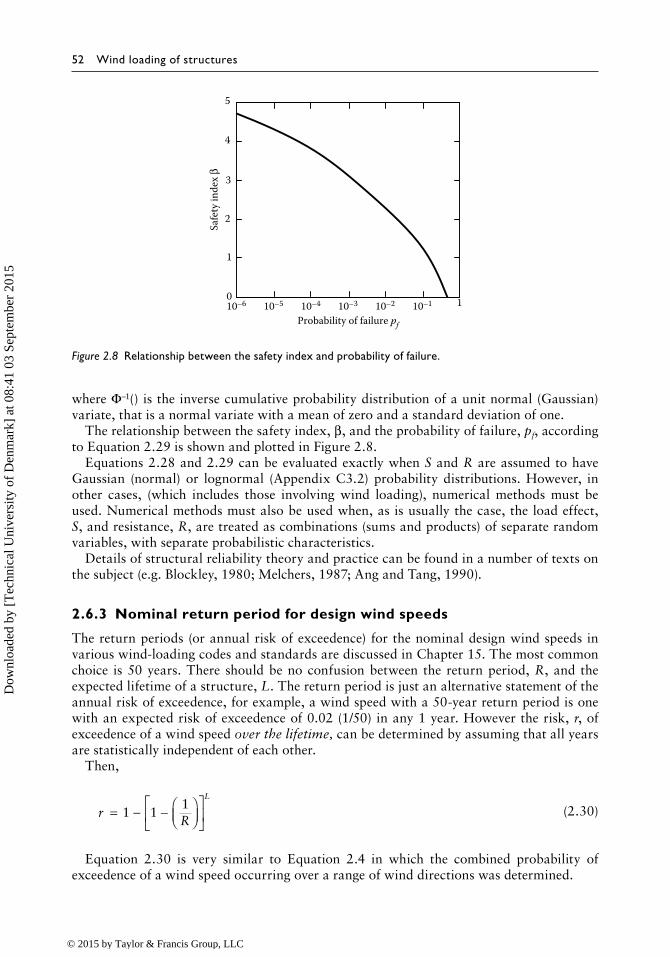
β = − Φ−1 (pf) (2.29)
S (load effect)
fs(S) · δS
δSS
R (resistance)
R S, R
FR(S)
FS(S)
FR(R)
Figure 2.7 Probability densities for load effects and resistance.
where Φ−1() is the inverse cumulative probability distribution of a unit normal (Gaussian) variate, that is a normal variate with a mean of zero and a standard deviation of one.
The relationship between the safety index, β, and the probability of failure, pf, according to Equation 2.29 is shown and plotted in Figure 2.8.
Equations 2.28 and 2.29 can be evaluated exactly when S and R are assumed to have Gaussian (normal) or lognormal (Appendix C3.2) probability distributions. However, in other cases, (which includes those involving wind loading), numerical methods must be used. Numerical methods must also be used when, as is usually the case, the load effect, S, and resistance, R, are treated as combinations (sums and products) of separate random variables, with separate probabilistic characteristics.
Details of structural reliability theory and practice can be found in a number of texts on the subject (e.g. Blockley, 1980; Melchers, 1987; Ang and Tang, 1990).
2.6.3 nominal return period for design wind speeds
The return periods (or annual risk of exceedence) for the nominal design wind speeds in various wind-loading codes and standards are discussed in Chapter 15. The most common choice is 50 years. There should be no confusion between the return period, R, and the expected lifetime of a structure, L. The return period is just an alternative statement of the annual risk of exceedence, for example, a wind speed with a 50-year return period is one with an expected risk of exceedence of 0.02 (1/50) in any 1 year. However the risk, r, of exceedence of a wind speed over the lifetime, can be determined by assuming that all years are statistically independent of each other.
Then,
r
R
L
= −
1 1
1−
(2.30)
Equation 2.30 is very similar to Equation 2.4 in which the combined probability of exceedence of a wind speed occurring over a range of wind directions was determined.
5
4
3
2Sa
fety
inde
x β
1
010–6 10–5 10–4 10–3
Probability of failure pf
10–2 10–1 1
Figure 2.8 Relationship between the safety index and probability of failure.
Prediction of design wind speeds and structural safety 53
Setting both R and L as 50 years in Equation 2.30, we arrive at a value of r of 0.636. Thus, there is a nearly 64% chance that the 50-year return period wind speed will be exceeded at least once during a 50-year lifetime – that is a better than even chance that it will occur. Wind loads derived from wind speeds with this level of risk must be factored up when used for the ultimate limit states design. Typical values of the wind load factor, γW, are in the range of 1.4–1.6. Different values may be required for regions with different wind speed/return period relationships, as discussed in Section 2.7.
The use of a return period for the nominal design wind speed, substantially higher than the traditional 50 years, avoids the need to have different wind load factors in different regions. This was an important consideration in the revision of the Australian Standard for Wind Loads in 1989 (Standards Australia, 1989), which, in previous editions, required the use of a special ‘Cyclone Factor’ in the regions of northern coastline affected by tropical cyclones. The reason for this factor was the greater rate of change of wind speed with return period in the cyclone regions. A similar ‘hurricane importance factor’ appeared in some edi-tions of the American National Standard (ASCE, 1993), but was later incorporated into the specified basic wind speed (ASCE, 1998).
In AS1170.2-1989, the wind speeds for ultimate limit states design had a nominal probability of exceedence of 5% in a lifetime of 50 years (a return period of 1000 years, approximately).
However, a load factor of 1.0 was applied to the wind loads derived in this way – and this factor was the same in both cyclonic and non-cyclonic regions.
2.6.4 uncertainties in wind load specifications
A reliability study of structural design involving wind loads requires an estimation of all the uncertainties involved in the specification of wind loads – wind speeds, multipliers for the terrain height and topography, pressure coefficients, local and area-averaging effects and so on. Some examples of this type of study for buildings and communication towers were given by Pham et al. (1983, 1992).
Table 2.7 shows estimates by Pham et al. (1983) of mean-to-nominal values of vari-ous parameters associated with wind-loading calculations for regions affected by tropical cyclones from the Australian Standard of that time. It can be seen from Table 2.7 that the greatest contributor to the variability and uncertainty in wind load estimation is the wind speed itself – particularly as it is raised to a power of 2 (or greater, when dynamic effects are important) when wind loads and effects are calculated. A secondary contributor is the uncertainty in the exposure parameter in Table 2.7, which is also squared, and includes uncertainties in the vertical profile of mean and gust speeds as discussed in the earlier sec-tions of this chapter.
Table 2.7 Variability of wind-loading parameters
Parameter Mean/nominal Coefficient of variation Assumed distribution
Source: Reprinted from Journal of Wind Engineering and Industrial Aerodynamics, Pham, L., Holmes, J.D. and Leicester, R.H., Safety indices for wind loading in Australia, 14: 3–14, Copyright 1983, with permission from Elsevier.
As discussed in the previous section, wind load factors, γw, in the range of 1.4–1.6 have traditionally been adopted for use with wind loads derived on the basis of a 50-year return period wind speeds. Wind load factors in this range have been derived on the basis of two assumptions:
1. Wind loads vary as the square of wind speeds. This is valid for small structures of high frequency with high natural frequencies. However, this assumption is not valid for tall buildings for which the effective wind loads vary to a higher power of wind speed, due to the effect of a resonant dynamic response. This power is up to 2.5 for a long-wind response, and up to 3 for cross-wind response (see Chapter 9).
2. The wind load factors have been derived for non-tropical-cyclone wind loads, that is cli-mates for which the rate of change of wind speed with return period R is relatively low, compared with those in regions affected by tropical cyclones, typhoons or hurricanes.
For structures with a significant dynamic response to wind such as tall buildings, wind loads and effects vary with wind speed raised to a power somewhat greater than 2. Holmes and Pham (1993) considered the effect of the varying exponent on the safety index and showed that the use of the traditional approach of ‘working stress’ wind loads based on a 50-year return period wind speed, with a fixed wind load factor of 1.5, resulted in a signifi-cant reduction in safety as the exponent increased. However, a near-uniform safety (insen-sitive to the effects of dynamic response) was achieved by the use of a high return period nominal design wind speed together with a wind load factor of 1.0.
The need for higher load factors in locations affected by tropical cyclones is illustrated by Table 2.8. This shows the equivalent return period of wind speeds when a wind load factor of 1.4 is applied to the 50-year return period value for several different locations. For two locations in the United Kingdom, the application of the 1.4 factor is equivalent to calculat-ing wind loads from wind speeds with return periods considerably greater than 1000 years. However, in Penang, Malaysia, where design wind speeds are governed by winds from rela-tively infrequent severe thunderstorms, the factor of 1.4 is equivalent to using a wind speed of about 500 years return period.
At Port Hedland (Western Australia), and Hong Kong, where tropical cyclones and typhoons are dominant, and extreme wind events are even rarer, the factored wind load based on V50 is equivalent to applying wind loads of only 150 and 220 years return period, respectively. In Australia, previous editions of AS1170.2 adjusted the effective return period by use of the ‘Cyclone Factor’ as discussed above. However, in AS/NZS1170:2010,
Table 2.8 Return periods of factored wind loads with a wind load factor of 1.4
Note: (i) Values of wind speed shown are gust speeds at 10-m height over a flat open terrain, except for Hong Kong for which the gust speed is adjusted to 50-m height above the ocean. (ii) Probability distributions for Cardington and Jersey obtained from Cook, N.J. 1985. The Designer’s Guide to Wind Loading of Building Structures. BRE-Butterworths, UK.
Prediction of design wind speeds and structural safety 55
a nominal design wind speed with 500 years return period (80 m/s basic gust wind speed at Port Hedland) with a wind load factor of 1.0 is used for the design of most structures for ultimate limit states. An ‘uncertainty’ factor of 1.10 is also applied to the wind speeds in that part of Australia, further increasing the effective return period based on recorded data.
2.8 suMMary
In this chapter, the application of extreme value analysis to the prediction of design wind speeds has been discussed. In particular, the Gumbel and ‘peaks over threshold’ approaches were described in detail. The need to separate wind speeds caused by wind storms of differ-ent types was emphasised, and wind direction effects were considered.
The main principles of the application of probability to the structural design and safety under wind loads were also introduced.
reFerences
American Society of Civil Engineers. 1993. Minimum Design Loads for Buildings and Other Structures. ASCE Standard, ANSI/ASCE 7-93, American Society of Civil Engineers, New York.
American Society of Civil Engineers. 1998. Minimum Design Loads for Buildings and Other Structures. ASCE Standard, ANSI/ASCE 7-98, American Society of Civil Engineers, New York.
American Society of Civil Engineers. 2010. Minimum Design Loads for Buildings and Other Structures. ASCE/SEI 7-10, American Society of Civil Engineers, New York.
Ang, A.H. and Tang, W. 1990. Probability Concepts in Engineering Planning and Design. Vol. II. Decision, Risk and Reliability. Published by the authors.
Blockley, D. 1980. The Nature of Structural Design and Safety. Ellis Horwood, Chichester, England, UK.Cook, N.J. 1983. Note on directional and seasonal assessment of extreme wind speeds for design.
Journal of Wind Engineering and Industrial Aerodynamics, 12: 365–72.Cook, N.J. 1985. The Designer’s Guide to Wind Loading of Building Structures. BRE-Butterworths, UK.Cook, N.J. and Harris, R.I. 2004. Exact and general FT1 penultimate distributions of extreme winds
drawn from tail-equivalent Weibull parents. Structural Safety, 26: 391–420.Cook, N.J. and Miller, C.A.M. 1999. Further note on directional assessment of extreme wind speeds for
design. Journal of Wind Engineering and Industrial Aerodynamics, 79: 201–8.Davenport, A.G. 1961. The application of statistical concepts to the wind loading of structures.
Proceedings Institution of Civil Engineers, 19: 449–71.Davison, A.C. and Smith, R.L. 1990. Models for exceedances over high thresholds. Journal of the Royal
Statistical Society, Series B, 52: 339–442.Fisher, R.A. and Tippett, L.H.C. 1928. Limiting forms of the frequency distribution of the largest or
smallest member of a sample. Proceedings, Cambridge Philosophical Society Part 2, 24: 180–90.Freudenthal, A.M. 1947. The safety of structures. American Society of Civil Engineers Transactions,
112: 125–59.Freudenthal, A.M. 1956. Safety and the probability of structural failure. American Society of Civil
Engineers Transactions, 121: 1337–97.Gomes, L. and Vickery, B.J. 1977a. Extreme wind speeds in mixed wind climates. Journal of Industrial
Aerodynamics, 2: 331–44.Gomes, L. and Vickery, B.J. 1977b. On the prediction of extreme wind speeds from the parent distribu-
tion. Journal of Industrial Aerodynamics, 2: 21–36.Gringorten, I.I. 1963. A plotting rule for extreme probability paper. Journal of Geophysical Research,
68: 813–4.Gumbel, E.J. 1954. Statistical Theory of Extreme Values and Some Practical Applications. Applied
Math Series 33, National Bureau of Standards, Washington, DC.
Gumbel, E.J. 1958. Statistics of Extremes. Columbia University Press, New York.Holmes, J.D. 1990. Directional effects on extreme wind loads. Civil Engineering Transactions,
Institution of Engineers, Australia, 32: 45–50.Holmes, J.D. 2002. A re-analysis of recorded extreme wind speeds in Region A. Australian Journal of
Structural Engineering, 4: 29–40.Holmes, J.D. and Ginger, J.D. 2012. The gust wind speed duration in AS/NZS 1170.2. Australian
Journal of Structural Engineering (I.E. Aust.), 13: 207–17.Holmes, J.D. and Moriarty, W.W. 1999. Application of the generalized Pareto distribution to extreme
value analysis in wind engineering. Journal of Wind Engineering and Industrial Aerodynamics, 83: 1–10.
Holmes, J.D. and Moriarty, W.W. 2001. Response to discussion by N.J. Cook and R.I. Harris of: Application of the generalized Pareto distribution to extreme value analysis in wind engineering. Journal of Wind Engineering and Industrial Aerodynamics, 89: 225–7.
Holmes, J.D. and Pham, L. 1993. Wind-induced dynamic response and the safety index. Proceedings of the 6th International Conference on Structural Safety and Reliability, Innsbruck, Austria, 9–13 August, pp. 1707–9, A.A. Balkema Publishers.
Hosking, J.R.M., Wallis, J.R. and Wood, E.F. 1985. Estimates of the generalized extreme value distribu-tion by the method of probability-weighted moments. Technometrics, 27: 251–61.
Jenkinson, A.F. 1955. The frequency distribution of the annual maximum (or minimum) values of meteorological elements. Quarterly Journal of the Royal Meteorological Society, 81: 158–71.
Kasperski, M. 2007. Design wind speeds for a low-rise building taking into account directional effects. Journal of Wind Engineering and Industrial Aerodynamics, 95: 1125–44.
Lechner, J.A., Leigh, S.D. and Simiu, E. 1992. Recent approaches to extreme value estimation with application to wind speeds. Part 1: The Pickands method. Journal of Wind Engineering and Industrial Aerodynamics, 41: 509–19.
Lieblein, J. 1974. Efficient methods of extreme-value methodology. Report NBSIR 74-602, National Bureau of Standards, Washington.
Melbourne, W.H. 1984. Designing for directionality. Workshop on Wind Engineering and Industrial Aerodynamics, Highett, Victoria, Australia, July.
Melchers, R. 1987. Structural Reliability – Analysis and Prediction. Ellis Horwood, Chichester, England, UK.
Miller, C.A., Holmes, J.D., Henderson, D.J., Ginger, J.D. and Morrison, M. 2013. The response of the Dines anemometer to gusts and comparisons with cup anemometers. Journal of Atmospheric and Oceanic Technology, 30: 1320–36.
Palutikof, J.P., Brabson, B.B., Lister, D.H. and Adcock, S.T. 1999. A review of methods to calculate extreme wind speeds. Meteorological Applications, 6: 119–32.
Peterka, J.A. and Shahid, S. 1998. Design gust wind speeds in the United States. Journal of Structural Engineering (ASCE), 124: 207–14.
Pham, L., Holmes, J.D. and Leicester, R.H. 1983. Safety indices for wind loading in Australia. Journal of Wind Engineering and Industrial Aerodynamics, 14: 3–14.
Pham, L., Holmes, J.D. and Yang, J. 1992. Reliability analysis of Australian communication lattice tow-ers. Journal of Constructional Steel Research, 23: 255–72.
Pugsley, A.G. 1966. The Safety of Structures. Edward Arnold, London.Russell, L.R. 1971. Probabilistic distributions for hurricane effects. American Society of Civil Enginners
Journal of Waterways, Harbours and Coastal Engineering, 97: 139–54.Standards Australia. 1989. SAA Loading Code. Part 2: Wind Loads. Standards Australia, North Sydney,
New South Wales, Australia. Australian Standard AS1170.2-1989.Standards Australia. 2011. Structural Design Actions. Part 2: Wind Actions. Standards Australia,
Sydney, New South Wales, Australia. Australian/New Zealand Standard, AS/NZS1170.2:2011.Von Mises, R. 1936. La Distribution de la Plus Grande de n Valeurs. Reprinted in Selected Papers of
Richard von Mises, 2: 271–94, American Mathematical Society, Providence R.I., USA.