BACHELOR THESIS IN AERONAUTICAL …432360/FULLTEXT01.pdfBACHELOR THESIS IN AERONAUTICAL ENGINEERING...

BACHELOR THESIS IN AERONAUTICAL ENGINEERING 15 CREDITS, BASIC LEVEL 300

School of Innovation, Design and Engineering

Aerodynamic Investigation of Air Inlets on Aircrafts with Application of Computational Fluid Dynamics

Author: Marcus Lejon Report code: MDH.IDT.FLYG.0233.2011.GN300.15HP.Ae

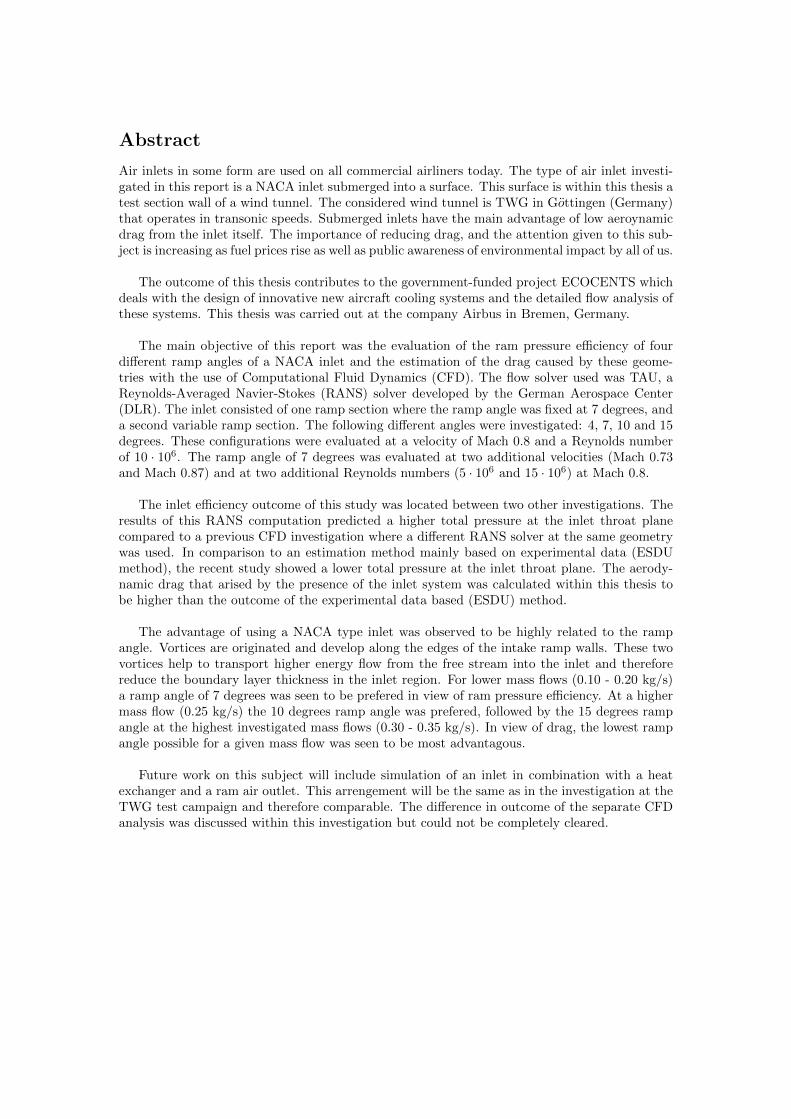
Abstract

Air inlets in some form are used on all commercial airliners today. The type of air inlet investi-gated in this report is a NACA inlet submerged into a surface. This surface is within this thesis atest section wall of a wind tunnel. The considered wind tunnel is TWG in Gottingen (Germany)that operates in transonic speeds. Submerged inlets have the main advantage of low aeroynamicdrag from the inlet itself. The importance of reducing drag, and the attention given to this sub-ject is increasing as fuel prices rise as well as public awareness of environmental impact by all of us.

The outcome of this thesis contributes to the government-funded project ECOCENTS whichdeals with the design of innovative new aircraft cooling systems and the detailed flow analysis ofthese systems. This thesis was carried out at the company Airbus in Bremen, Germany.

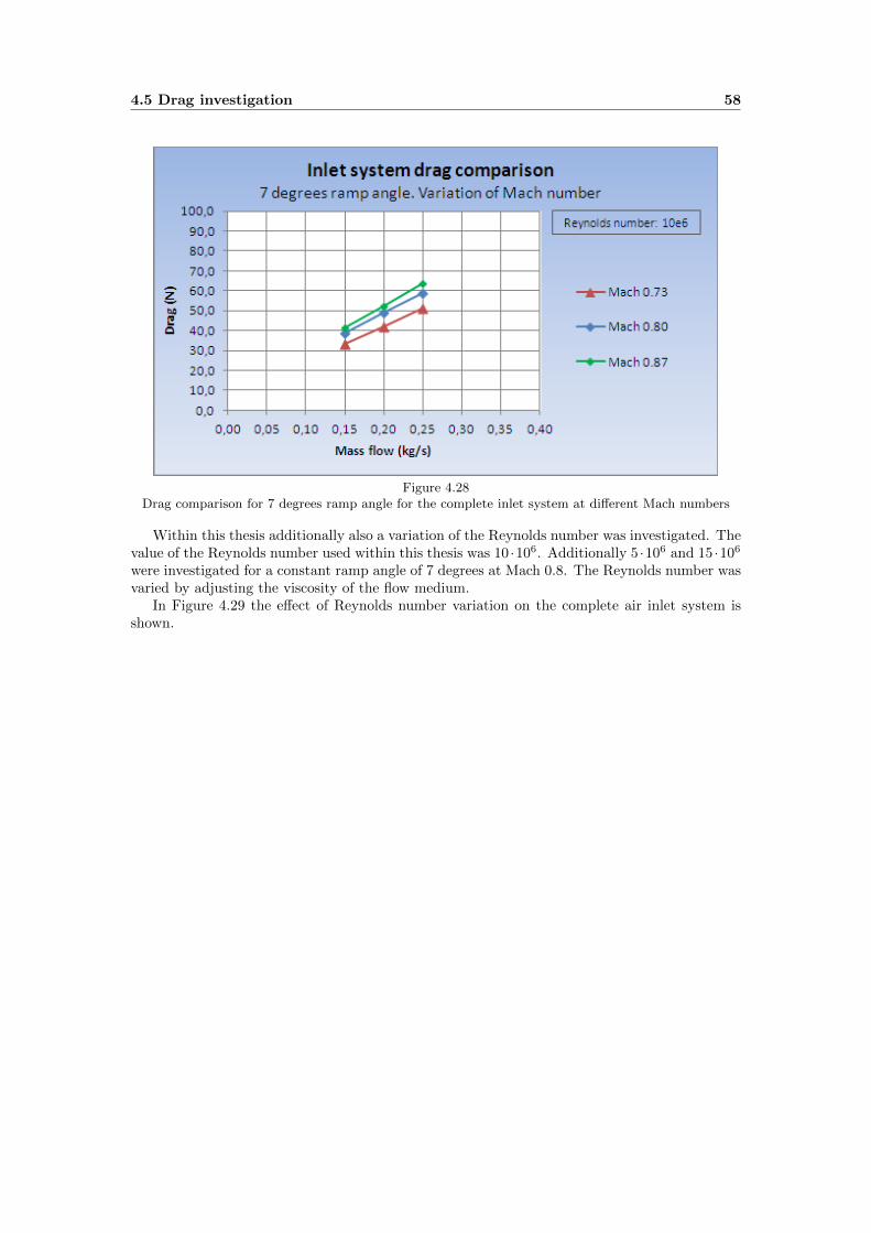
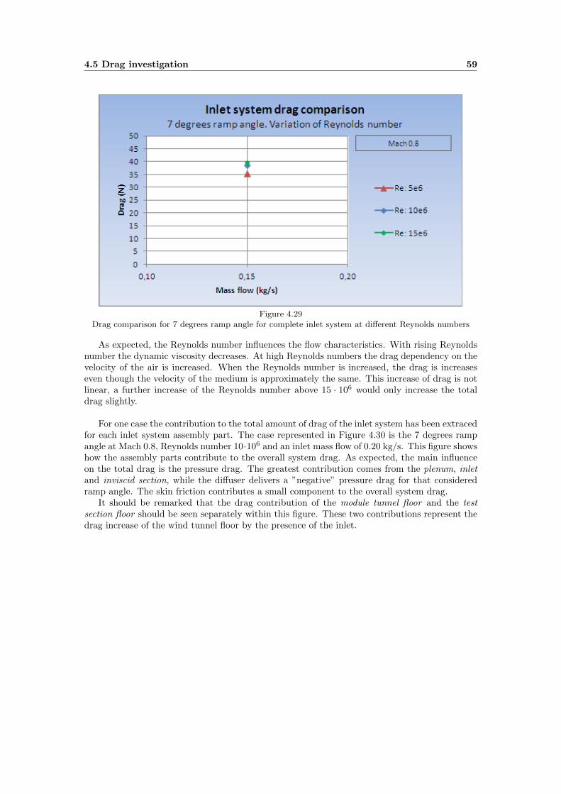
The main objective of this report was the evaluation of the ram pressure efficiency of fourdifferent ramp angles of a NACA inlet and the estimation of the drag caused by these geome-tries with the use of Computational Fluid Dynamics (CFD). The flow solver used was TAU, aReynolds-Averaged Navier-Stokes (RANS) solver developed by the German Aerospace Center(DLR). The inlet consisted of one ramp section where the ramp angle was fixed at 7 degrees, anda second variable ramp section. The following different angles were investigated: 4, 7, 10 and 15degrees. These configurations were evaluated at a velocity of Mach 0.8 and a Reynolds numberof 10 · 106. The ramp angle of 7 degrees was evaluated at two additional velocities (Mach 0.73and Mach 0.87) and at two additional Reynolds numbers (5 · 106 and 15 · 106) at Mach 0.8.

The inlet efficiency outcome of this study was located between two other investigations. Theresults of this RANS computation predicted a higher total pressure at the inlet throat planecompared to a previous CFD investigation where a different RANS solver at the same geometrywas used. In comparison to an estimation method mainly based on experimental data (ESDUmethod), the recent study showed a lower total pressure at the inlet throat plane. The aerody-namic drag that arised by the presence of the inlet system was calculated within this thesis tobe higher than the outcome of the experimental data based (ESDU) method.

The advantage of using a NACA type inlet was observed to be highly related to the rampangle. Vortices are originated and develop along the edges of the intake ramp walls. These twovortices help to transport higher energy flow from the free stream into the inlet and thereforereduce the boundary layer thickness in the inlet region. For lower mass flows (0.10 - 0.20 kg/s)a ramp angle of 7 degrees was seen to be prefered in view of ram pressure efficiency. At a highermass flow (0.25 kg/s) the 10 degrees ramp angle was prefered, followed by the 15 degrees rampangle at the highest investigated mass flows (0.30 - 0.35 kg/s). In view of drag, the lowest rampangle possible for a given mass flow was seen to be most advantagous.

Future work on this subject will include simulation of an inlet in combination with a heatexchanger and a ram air outlet. This arrengement will be the same as in the investigation at theTWG test campaign and therefore comparable. The difference in outcome of the separate CFDanalysis was discussed within this investigation but could not be completely cleared.

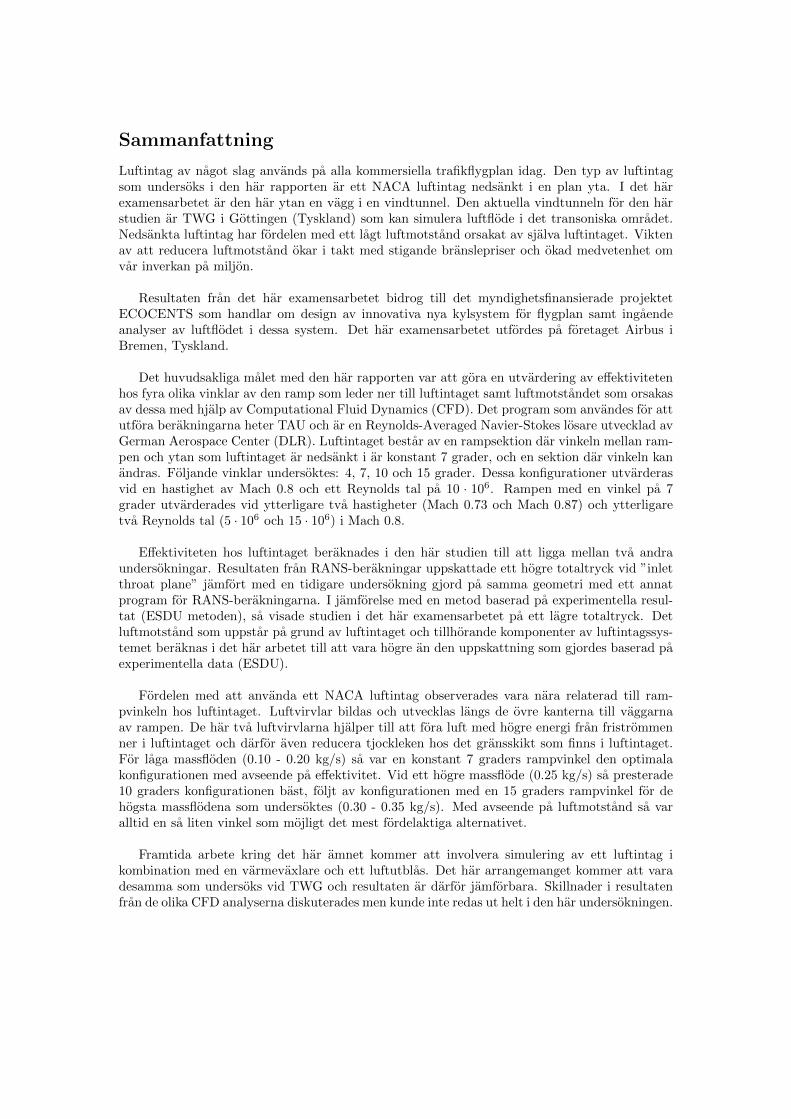
Sammanfattning

Luftintag av nagot slag anvands pa alla kommersiella trafikflygplan idag. Den typ av luftintagsom undersoks i den har rapporten ar ett NACA luftintag nedsankt i en plan yta. I det harexamensarbetet ar den har ytan en vagg i en vindtunnel. Den aktuella vindtunneln for den harstudien ar TWG i Gottingen (Tyskland) som kan simulera luftflode i det transoniska omradet.Nedsankta luftintag har fordelen med ett lagt luftmotstand orsakat av sjalva luftintaget. Viktenav att reducera luftmotstand okar i takt med stigande branslepriser och okad medvetenhet omvar inverkan pa miljon.

Resultaten fran det har examensarbetet bidrog till det myndighetsfinansierade projektetECOCENTS som handlar om design av innovativa nya kylsystem for flygplan samt ingaendeanalyser av luftflodet i dessa system. Det har examensarbetet utfordes pa foretaget Airbus iBremen, Tyskland.

Det huvudsakliga malet med den har rapporten var att gora en utvardering av effektivitetenhos fyra olika vinklar av den ramp som leder ner till luftintaget samt luftmotstandet som orsakasav dessa med hjalp av Computational Fluid Dynamics (CFD). Det program som anvandes for attutfora berakningarna heter TAU och ar en Reynolds-Averaged Navier-Stokes losare utvecklad avGerman Aerospace Center (DLR). Luftintaget bestar av en rampsektion dar vinkeln mellan ram-pen och ytan som luftintaget ar nedsankt i ar konstant 7 grader, och en sektion dar vinkeln kanandras. Foljande vinklar undersoktes: 4, 7, 10 och 15 grader. Dessa konfigurationer utvarderasvid en hastighet av Mach 0.8 och ett Reynolds tal pa 10 · 106. Rampen med en vinkel pa 7grader utvarderades vid ytterligare tva hastigheter (Mach 0.73 och Mach 0.87) och ytterligaretva Reynolds tal (5 · 106 och 15 · 106) i Mach 0.8.

Effektiviteten hos luftintaget beraknades i den har studien till att ligga mellan tva andraundersokningar. Resultaten fran RANS-berakningar uppskattade ett hogre totaltryck vid ”inletthroat plane” jamfort med en tidigare undersokning gjord pa samma geometri med ett annatprogram for RANS-berakningarna. I jamforelse med en metod baserad pa experimentella resul-tat (ESDU metoden), sa visade studien i det har examensarbetet pa ett lagre totaltryck. Detluftmotstand som uppstar pa grund av luftintaget och tillhorande komponenter av luftintagssys-temet beraknas i det har arbetet till att vara hogre an den uppskattning som gjordes baserad paexperimentella data (ESDU).

Fordelen med att anvanda ett NACA luftintag observerades vara nara relaterad till ram-pvinkeln hos luftintaget. Luftvirvlar bildas och utvecklas langs de ovre kanterna till vaggarnaav rampen. De har tva luftvirvlarna hjalper till att fora luft med hogre energi fran fristrommenner i luftintaget och darfor aven reducera tjockleken hos det gransskikt som finns i luftintaget.For laga massfloden (0.10 - 0.20 kg/s) sa var en konstant 7 graders rampvinkel den optimalakonfigurationen med avseende pa effektivitet. Vid ett hogre massflode (0.25 kg/s) sa presterade10 graders konfigurationen bast, foljt av konfigurationen med en 15 graders rampvinkel for dehogsta massflodena som undersoktes (0.30 - 0.35 kg/s). Med avseende pa luftmotstand sa varalltid en sa liten vinkel som mojligt det mest fordelaktiga alternativet.

Framtida arbete kring det har amnet kommer att involvera simulering av ett luftintag ikombination med en varmevaxlare och ett luftutblas. Det har arrangemanget kommer att varadesamma som undersoks vid TWG och resultaten ar darfor jamforbara. Skillnader i resultatenfran de olika CFD analyserna diskuterades men kunde inte redas ut helt i den har undersokningen.

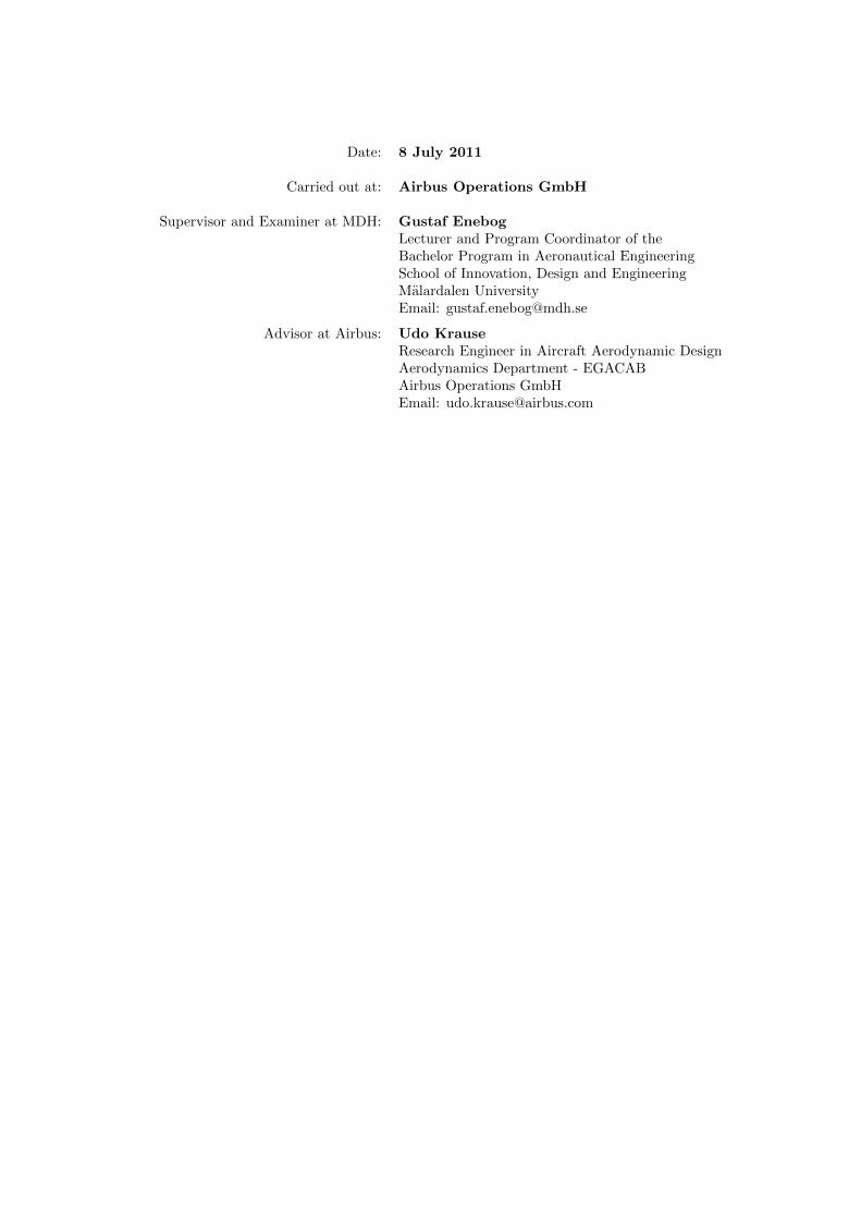
Date: 8 July 2011

Carried out at: Airbus Operations GmbH

Supervisor and Examiner at MDH: Gustaf EnebogLecturer and Program Coordinator of theBachelor Program in Aeronautical EngineeringSchool of Innovation, Design and EngineeringMalardalen UniversityEmail: [email protected]

Advisor at Airbus: Udo KrauseResearch Engineer in Aircraft Aerodynamic DesignAerodynamics Department - EGACABAirbus Operations GmbHEmail: [email protected]

Acknowledgements

I would like to thank Udo Krause for all his help with this thesis and for making me feel verywelcome to Germany and the Airbus company.

Thank you to Bruno Stefes who shared his expertise on intakes and aerodynamics in general.

Thank you to everyone at the Aerodynamics department at Airbus in Bremen for being veryfriendly and giving me a good place to perform my studies.

Thank you to Linda van Leeuwen, my partner, who has been very supportive during this under-taking.

vi

Contents

Abbreviations viii

Symbols and Subscripts ix

List of Tables x

List of Figures xi

1 Introduction 11.1 Background . . . . . . . . . . . . . . . . . . . . . . . . . . . . . . . . . . . . . . . 1

1.1.1 Project ECOcents . . . . . . . . . . . . . . . . . . . . . . . . . . . . . . . 21.2 Purpose . . . . . . . . . . . . . . . . . . . . . . . . . . . . . . . . . . . . . . . . . 31.3 Scope of work . . . . . . . . . . . . . . . . . . . . . . . . . . . . . . . . . . . . . . 5

2 Theory 72.1 Boundary Layer Theory . . . . . . . . . . . . . . . . . . . . . . . . . . . . . . . . 72.2 Drag . . . . . . . . . . . . . . . . . . . . . . . . . . . . . . . . . . . . . . . . . . . 82.3 Flight Mechanics . . . . . . . . . . . . . . . . . . . . . . . . . . . . . . . . . . . . 92.4 Ram Pressure Efficiency . . . . . . . . . . . . . . . . . . . . . . . . . . . . . . . . 102.5 Ram Recovery Ratio . . . . . . . . . . . . . . . . . . . . . . . . . . . . . . . . . . 102.6 Mass Flow Ratio . . . . . . . . . . . . . . . . . . . . . . . . . . . . . . . . . . . . 102.7 Navier-Stokes Equations . . . . . . . . . . . . . . . . . . . . . . . . . . . . . . . . 112.8 Reynolds-Averaged Navier-Stokes Equations . . . . . . . . . . . . . . . . . . . . . 122.9 Spatial Discretisation . . . . . . . . . . . . . . . . . . . . . . . . . . . . . . . . . . 13

2.9.1 Computational Grids . . . . . . . . . . . . . . . . . . . . . . . . . . . . . . 142.9.2 Discretisation Methods . . . . . . . . . . . . . . . . . . . . . . . . . . . . 152.9.3 Central and Upwind Schemes . . . . . . . . . . . . . . . . . . . . . . . . . 15

2.10 Time Discretisation . . . . . . . . . . . . . . . . . . . . . . . . . . . . . . . . . . . 16

3 Methodology 173.1 Preliminary Studies . . . . . . . . . . . . . . . . . . . . . . . . . . . . . . . . . . 17

3.1.1 Inlets . . . . . . . . . . . . . . . . . . . . . . . . . . . . . . . . . . . . . . 173.1.2 Flush Inlets . . . . . . . . . . . . . . . . . . . . . . . . . . . . . . . . . . . 173.1.3 NACA Curved-Divergent Inlet . . . . . . . . . . . . . . . . . . . . . . . . 193.1.4 Design Parameters . . . . . . . . . . . . . . . . . . . . . . . . . . . . . . . 213.1.5 Inlet Drag . . . . . . . . . . . . . . . . . . . . . . . . . . . . . . . . . . . . 243.1.6 Plenums . . . . . . . . . . . . . . . . . . . . . . . . . . . . . . . . . . . . . 26

3.2 Geometry Preparation . . . . . . . . . . . . . . . . . . . . . . . . . . . . . . . . . 273.3 Mesh Generation . . . . . . . . . . . . . . . . . . . . . . . . . . . . . . . . . . . . 293.4 Numerical Computation . . . . . . . . . . . . . . . . . . . . . . . . . . . . . . . . 333.5 Post Processing . . . . . . . . . . . . . . . . . . . . . . . . . . . . . . . . . . . . . 373.6 Empirical Method Analysis . . . . . . . . . . . . . . . . . . . . . . . . . . . . . . 39

4 Results and Discussion 414.1 Pressure and Mach number Analysis . . . . . . . . . . . . . . . . . . . . . . . . . 414.2 Boundary Layer Analysis . . . . . . . . . . . . . . . . . . . . . . . . . . . . . . . 43

4.2.1 Ramp wall edges . . . . . . . . . . . . . . . . . . . . . . . . . . . . . . . . 494.3 Ram Pressure Efficiency . . . . . . . . . . . . . . . . . . . . . . . . . . . . . . . . 50

vii

4.4 Ram Recovery Ratio . . . . . . . . . . . . . . . . . . . . . . . . . . . . . . . . . . 534.5 Drag investigation . . . . . . . . . . . . . . . . . . . . . . . . . . . . . . . . . . . 544.6 Internal Air Duct After the Plenum . . . . . . . . . . . . . . . . . . . . . . . . . 614.7 Analysis of the Vortices Formed by the NACA Inlet . . . . . . . . . . . . . . . . 634.8 Conclusions and Recommendations of Future Work . . . . . . . . . . . . . . . . . 67

References 70

A APPENDIX 71A.1 Computational Models and Tools . . . . . . . . . . . . . . . . . . . . . . . . . . . 71

A.1.1 CENTAUR . . . . . . . . . . . . . . . . . . . . . . . . . . . . . . . . . . . 71A.1.2 TAU . . . . . . . . . . . . . . . . . . . . . . . . . . . . . . . . . . . . . . . 75A.1.3 Tau BL . . . . . . . . . . . . . . . . . . . . . . . . . . . . . . . . . . . . . 75A.1.4 CATIA . . . . . . . . . . . . . . . . . . . . . . . . . . . . . . . . . . . . . 76A.1.5 Tecplot 360 . . . . . . . . . . . . . . . . . . . . . . . . . . . . . . . . . . . 76A.1.6 RAMAIR . . . . . . . . . . . . . . . . . . . . . . . . . . . . . . . . . . . . 76

A.2 Figures . . . . . . . . . . . . . . . . . . . . . . . . . . . . . . . . . . . . . . . . . 77A.2.1 Introduction . . . . . . . . . . . . . . . . . . . . . . . . . . . . . . . . . . 77A.2.2 Measurements . . . . . . . . . . . . . . . . . . . . . . . . . . . . . . . . . 79A.2.3 Geometry Preparation . . . . . . . . . . . . . . . . . . . . . . . . . . . . . 84A.2.4 Mesh Generation . . . . . . . . . . . . . . . . . . . . . . . . . . . . . . . . 86A.2.5 Post Processing . . . . . . . . . . . . . . . . . . . . . . . . . . . . . . . . . 88A.2.6 Results and Discussion . . . . . . . . . . . . . . . . . . . . . . . . . . . . . 96

A.3 Lessons Learned and Best Practice Settings . . . . . . . . . . . . . . . . . . . . . 101A.3.1 Mesh Generation . . . . . . . . . . . . . . . . . . . . . . . . . . . . . . . . 101A.3.2 Numerical Computation . . . . . . . . . . . . . . . . . . . . . . . . . . . . 110

A.4 Calculations . . . . . . . . . . . . . . . . . . . . . . . . . . . . . . . . . . . . . . . 111A.5 Tables . . . . . . . . . . . . . . . . . . . . . . . . . . . . . . . . . . . . . . . . . . 114A.6 Transonic Wind tunnel Gottingen . . . . . . . . . . . . . . . . . . . . . . . . . . . 116A.7 Input Files . . . . . . . . . . . . . . . . . . . . . . . . . . . . . . . . . . . . . . . 117

A.7.1 CENTAUR . . . . . . . . . . . . . . . . . . . . . . . . . . . . . . . . . . . 117A.7.2 TAU . . . . . . . . . . . . . . . . . . . . . . . . . . . . . . . . . . . . . . . 118A.7.3 Others . . . . . . . . . . . . . . . . . . . . . . . . . . . . . . . . . . . . . . 131

viii

Abbreviations

BL Boundary LayerCAD Computer Aided Design

CATIA Computer Aided Threedimensional Interactive Application(a commercial CAD software)

CFD Computational Fluid DynamicsCSM Computational Solid MechanicsDLR German Aerospace Center

ECOCENTS Efficient Cooling Center for Aircraft SystemsESDU Engineering Sciences Data Unit

FOD Foreign Object DamageNACA National Advisory Committee for Aeronautics

NS Navier-Stokes (equations)NWB Low-Speed Wind tunnel Braunschweig

RANS Reynolds-Averaged Navier-Stokes (equations)TWG Transonic Wind tunnel Gottingen

ix

Symbols and Subscripts

Dimensionless CoefficientsCD Drag coefficientCL Lift coefficientcp Pressure coefficientcv Specific heat at constant volumedc Drag count. 1 drag count is equal to 0.0001 CD

Roman SymbolsA1 Inlet throat area

c The fuel consumptionct The thrust-specific fuel consumptionD The drag expressed in Newtone Internal energy due to random molecular motionL The lift expressed in Newton

PT0 Free stream total pressurePT1 Average total pressure at the inlet throat planep0 Free stream static pressureR The specific gas constantq0 Free stream dynamic pressureS The wing area of an aircraftT Flow temperatureV0 Free stream velocityV1 Inlet throat flow velocityW0 The weight of an aircraft with full fuel tanksW1 The weight of the aircraft with empty fuel tanksy+ Non-dimensional distance from a surface

Greek Symbolsα Angle of attackδ The boundary layer thicknessη Ram pressure efficiencyηp Propeller efficiencyρ0 Free stream flow densityρ1 Inlet throat flow densityτw The shear friction at the surface of a solidθ Boundary layer displacement thickness

x

List of Tables

Table Description Page

3.1 Ramp coordinates for NACA curved-divergent planform . . . . . . . 203.2 Inlet drag and ram pressure effciency estimated with the help of

ESDU paper 86002 . . . . . . . . . . . . . . . . . . . . . . . . . . . . . . . . . . . . . . . . . . . . 39A.4.1 -A.4.2 Ram pressure efficiency calculation tables . . . . . . . . . . . . . . . . . . . . . 108-109A.4.3 -A.4.8 Inlet drag calculation tables . . . . . . . . . . . . . . . . . . . . . . . . . . . . . . . . . . . 109-110A.5.1 Geometry for different ramp angles . . . . . . . . . . . . . . . . . . . . . . . . . . . . 111A.5.2 Diffuser angles for different ramp angles . . . . . . . . . . . . . . . . . . . . . . . 112

xi

List of Figures

Figure Description Page

1.1 Air cooling and supply system on an aircraft body . . . . . . . . . . . . . . . . . . . . . . . . . . . . . . 11.2 ECOCENTS Logo . . . . . . . . . . . . . . . . . . . . . . . . . . . . . . . . . . . . . . . . . . . . . . . . . . . . . . . . . . . . . . 21.3 NACA type flush inlet . . . . . . . . . . . . . . . . . . . . . . . . . . . . . . . . . . . . . . . . . . . . . . . . . . . . . . . . . . 31.4 Cross section of an inlet . . . . . . . . . . . . . . . . . . . . . . . . . . . . . . . . . . . . . . . . . . . . . . . . . . . . . . . . 32.1 Velocity profile through a boundary layer . . . . . . . . . . . . . . . . . . . . . . . . . . . . . . . . . . . . . . . 72.2 Boundary layer growth along a flat plate . . . . . . . . . . . . . . . . . . . . . . . . . . . . . . . . . . . . . . . 72.3 Forces . . . . . . . . . . . . . . . . . . . . . . . . . . . . . . . . . . . . . . . . . . . . . . . . . . . . . . . . . . . . . . . . . . . . . . . . . . 82.4 Balance of Forces for Steady Level Flight . . . . . . . . . . . . . . . . . . . . . . . . . . . . . . . . . . . . . . . 92.5 Flush Inlet Denotations . . . . . . . . . . . . . . . . . . . . . . . . . . . . . . . . . . . . . . . . . . . . . . . . . . . . . . . . 102.6 Rectangular grid segment . . . . . . . . . . . . . . . . . . . . . . . . . . . . . . . . . . . . . . . . . . . . . . . . . . . . . . 142.7 Unstructured grid segment . . . . . . . . . . . . . . . . . . . . . . . . . . . . . . . . . . . . . . . . . . . . . . . . . . . . . 143.1 Scoop inlet . . . . . . . . . . . . . . . . . . . . . . . . . . . . . . . . . . . . . . . . . . . . . . . . . . . . . . . . . . . . . . . . . . . . . 173.2 Flush inlet . . . . . . . . . . . . . . . . . . . . . . . . . . . . . . . . . . . . . . . . . . . . . . . . . . . . . . . . . . . . . . . . . . . . . 173.3 Flush inlets with convergent walls, divergent walls and parallel walls respectively 183.4 Vortices formed along the edges of a ush inlet with divergent walls . . . . . . . . . . . . . . 193.5 NACA curved-divergent planform . . . . . . . . . . . . . . . . . . . . . . . . . . . . . . . . . . . . . . . . . . . . . . 203.6 NACA curved-divergent inlet . . . . . . . . . . . . . . . . . . . . . . . . . . . . . . . . . . . . . . . . . . . . . . . . . . . 203.7 Arrangement of the submerged NACA inlet in Reference [14] . . . . . . . . . . . . . . . . . . . 213.8 Resulting change of the ramp from a change of ramp angle . . . . . . . . . . . . . . . . . . . . . 223.9 Surface parallel to the free stream and a ramp section . . . . . . . . . . . . . . . . . . . . . . . . . . 233.10 Deflectors . . . . . . . . . . . . . . . . . . . . . . . . . . . . . . . . . . . . . . . . . . . . . . . . . . . . . . . . . . . . . . . . . . . . . . 243.11 The effect of mass flow ratio on the entry streamtube . . . . . . . . . . . . . . . . . . . . . . . . . . . 253.12 Plenum classic . . . . . . . . . . . . . . . . . . . . . . . . . . . . . . . . . . . . . . . . . . . . . . . . . . . . . . . . . . . . . . . . . 263.13 Plenum base . . . . . . . . . . . . . . . . . . . . . . . . . . . . . . . . . . . . . . . . . . . . . . . . . . . . . . . . . . . . . . . . . . . 263.14 Original wind tunnel geometry . . . . . . . . . . . . . . . . . . . . . . . . . . . . . . . . . . . . . . . . . . . . . . . . . 273.15 The wind tunnel geometry with an extension aft of the test section . . . . . . . . . . . . . 273.16 The boundary of the module . . . . . . . . . . . . . . . . . . . . . . . . . . . . . . . . . . . . . . . . . . . . . . . . . . . 283.17 The module ready to be imported into CENTAUR . . . . . . . . . . . . . . . . . . . . . . . . . . . . . 283.18 The inlet system with coordinate axis . . . . . . . . . . . . . . . . . . . . . . . . . . . . . . . . . . . . . . . . . . 293.19 Illustration of the extension made to the duct prior to the outlet . . . . . . . . . . . . . . . . 293.20 Geometrical sources in the test section of the wind tunnel . . . . . . . . . . . . . . . . . . . . . . 303.21 Surface mesh at the inlet . . . . . . . . . . . . . . . . . . . . . . . . . . . . . . . . . . . . . . . . . . . . . . . . . . . . . . . 323.22 The contour of the prismatic layers inside the inlet . . . . . . . . . . . . . . . . . . . . . . . . . . . . . 313.23 The mesh at x = 135 . . . . . . . . . . . . . . . . . . . . . . . . . . . . . . . . . . . . . . . . . . . . . . . . . . . . . . . . . . . 323.24 The mesh at x = 180 . . . . . . . . . . . . . . . . . . . . . . . . . . . . . . . . . . . . . . . . . . . . . . . . . . . . . . . . . . . 323.25 The wind tunnel geometry with extensions . . . . . . . . . . . . . . . . . . . . . . . . . . . . . . . . . . . . . 333.26 Computational grid at the additional outlet . . . . . . . . . . . . . . . . . . . . . . . . . . . . . . . . . . . . 343.27 Velocity profiles at the additional outlet . . . . . . . . . . . . . . . . . . . . . . . . . . . . . . . . . . . . . . . . 343.28 Schematic set-up of the numerical wind tunnel simulation . . . . . . . . . . . . . . . . . . . . . . . 343.29 Close-up of the mesh at the wind tunnel test section . . . . . . . . . . . . . . . . . . . . . . . . . . . . 353.30 Side view of the wind tunnel showing the pressure distribution in Tecplot 360 . . . 373.31 Side view of the wind tunnel showing the Mach number in Tecplot 360 . . . . . . . . . 373.32 Residual plot for the clean wind tunnel setup . . . . . . . . . . . . . . . . . . . . . . . . . . . . . . . . . . . 383.33 Residual plot for the wind tunnel with an inlet . . . . . . . . . . . . . . . . . . . . . . . . . . . . . . . . . 38

xii


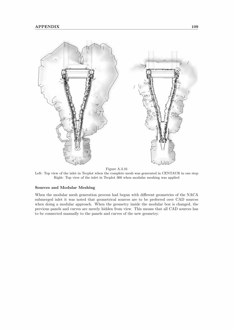
4.1 Side view in the symmetry plane of an inlet showing the Mach number . . . . . . . . . . 414.2 Side view in the symmetry plane of an inlet showing the Mach number . . . . . . . . . . 414.3 Side view in the symmetry plane of an inlet showing the static pressure . . . . . . . . . . 424.4 Side view in the symmetry plane of an inlet showing the total pressure . . . . . . . . . . 424.5 Top view of the inlet with the positions of the cuts shown in Figure 4.6 - 4.8 . . . . 434.6 Side view in the symmetry plane of the inlet with streamlines. Cut 1 . . . . . . . . . . . . 434.7 Side view in the symmetry plane of the inlet with streamlines. Cut 2 . . . . . . . . . . . . 434.8 Side view in the symmetry plane of the inlet with streamlines. Cut 3 . . . . . . . . . . . . 434.9 Side view of the inlet with points showing the positions investigated in

Tau BL and Tecplot 360 . . . . . . . . . . . . . . . . . . . . . . . . . . . . . . . . . . . . . . . . . . . . . . . . . . . . . . . . 444.10 Velocity profiles 260 mm prior to the inlet . . . . . . . . . . . . . . . . . . . . . . . . . . . . . . . . . . . . . . . 454.11 Velocity profiles 50 mm prior to the inlet . . . . . . . . . . . . . . . . . . . . . . . . . . . . . . . . . . . . . . . . 464.12 Velocity profiles 15 mm aft of the inlet lip . . . . . . . . . . . . . . . . . . . . . . . . . . . . . . . . . . . . . . . 464.13 Detailed velocity profile 15 mm aft of the inlet lip with the inlet present . . . . . . . . . 474.14 Velocity profiles 285 mm aft of the inlet lip . . . . . . . . . . . . . . . . . . . . . . . . . . . . . . . . . . . . . . 484.15 Velocity profile inside the inlet at the inlet throat plane . . . . . . . . . . . . . . . . . . . . . . . . . 484.16 Streamtraces placed at the NACA submerged inlet from a Tau BL solution

as seen in Tecplot 360 . . . . . . . . . . . . . . . . . . . . . . . . . . . . . . . . . . . . . . . . . . . . . . . . . . . . . . . . . . . 494.17 Ram pressure efficiency comparison at Mach 0.2 for different turbulence models . 504.18 Ram pressure efficiency comparison for different estimation methods . . . . . . . . . . . . . 514.19 Ram pressure efficiency comparison for different mass flows . . . . . . . . . . . . . . . . . . . . . . 524.20 Ram pressure efficiency for different inlet ramp angles in relation to the mass

flow . . . . . . . . . . . . . . . . . . . . . . . . . . . . . . . . . . . . . . . . . . . . . . . . . . . . . . . . . . . . . . . . . . . . . . . . . . . . . 524.21 Ram recovery ratio for different inlet ramp angles in relation to the mass flow . . . 534.22 Naming of the different inlet system assembly parts in this thesis . . . . . . . . . . . . . . . . 544.23 Naming of the wind tunnel test section parts in this thesis . . . . . . . . . . . . . . . . . . . . . . . 544.24 Drag comparison for the 7 degrees ramp angle configuration . . . . . . . . . . . . . . . . . . . . . 554.25 Drag comparison for the different ramp angles at Mach 0.8 . . . . . . . . . . . . . . . . . . . . . . 564.26 Side view in the symmetry plane of an inlet showing the Mach number . . . . . . . . . . 564.27 Drag comparison for the different angles for the complete inlet system at

Mach 0.8 . . . . . . . . . . . . . . . . . . . . . . . . . . . . . . . . . . . . . . . . . . . . . . . . . . . . . . . . . . . . . . . . . . . . . . . . 574.28 Drag comparison for 7 degrees ramp angle for the complete inlet system at

different Mach numbers . . . . . . . . . . . . . . . . . . . . . . . . . . . . . . . . . . . . . . . . . . . . . . . . . . . . . . . . . 584.29 Drag comparison for 7 degrees ramp angle for complete inlet system at

different Reynolds numbers . . . . . . . . . . . . . . . . . . . . . . . . . . . . . . . . . . . . . . . . . . . . . . . . . . . . . . 594.30 Drag contribution of different components of the inlet system and increase

of drag on surrounding floor panels. Percentage of total drag. . . . . . . . . . . . . . . . . . . . 604.31 -4.39 The inlet system and pressure plots in the inviscid section . . . . . . . . . . . . . . . . . . . . . . . 61-624.40 Plot of the vorticity at x-coordinate 135 for an inlet with 15 degrees ramp

angle. Streamtraces showing surrounding flow entering the inlet. . . . . . . . . . . . . . . . . 634.41 ISO Pressure-surface 73250 Pa. Mach 0.8. Reynolds number: 10e6 . . . . . . . . . . . . . . . 644.42 -4.45 Vorticity plots for 7 degrees ramp angle at Mach 0.8 and a mass flow of 0.20 kg/s 644.46 Inlet vorticity gradient . . . . . . . . . . . . . . . . . . . . . . . . . . . . . . . . . . . . . . . . . . . . . . . . . . . . . . . . . . 644.47 Sideview of the inlet system with x-positions . . . . . . . . . . . . . . . . . . . . . . . . . . . . . . . . . . . . 64

xiii


A.1.1 Control volume borders on a triangle . . . . . . . . . . . . . . . . . . . . . . . . . . . . . . . . . . . . . . . . . . . 72A.1.2 Control volume borders on a quadrilateral . . . . . . . . . . . . . . . . . . . . . . . . . . . . . . . . . . . . . . 72A.1.3 Control volume borders in a hexahedron . . . . . . . . . . . . . . . . . . . . . . . . . . . . . . . . . . . . . . . 73A.1.4 Control volume borders in a prism . . . . . . . . . . . . . . . . . . . . . . . . . . . . . . . . . . . . . . . . . . . . . 73A.1.5 Control volume borders in a tetrahedron . . . . . . . . . . . . . . . . . . . . . . . . . . . . . . . . . . . . . . . 75A.1.6 Control volume borders in a pyramid . . . . . . . . . . . . . . . . . . . . . . . . . . . . . . . . . . . . . . . . . . . 74A.1.7 Streaklines and the pressure distribution is visualised on a 2D view of a cylinder 76A.2.1 Example of an air cooling and supply system . . . . . . . . . . . . . . . . . . . . . . . . . . . . . . . . . . . 77A.2.2 Air cooling and supply system inside the belly fairing of an airplane . . . . . . . . . . . . 78A.2.3 Measurements of the NACA submerged inlet investigated in this report . . . . . . . . 79A.2.4 X-coordinates at different locations of the inlet . . . . . . . . . . . . . . . . . . . . . . . . . . . . . . . . . 79A.2.5 Side view of the wind tunnel geometry with measurements in millimeters . . . . . . . 80A.2.6 Side view of the wind tunnel test section with measurements in millimeters . . . . . 80A.2.7 Side view of the wind tunnel test section with measurements in millimeters . . . . . 81A.2.8 Top view of the wind tunnel test section with measurements in millimeters . . . . . 81A.2.9 Measurements in millimeters of the additional inlet geometry which was later

removed . . . . . . . . . . . . . . . . . . . . . . . . . . . . . . . . . . . . . . . . . . . . . . . . . . . . . . . . . . . . . . . . . . . . . . . 82A.2.10 Measurements in millimeters of the original and additional inlet geometry which

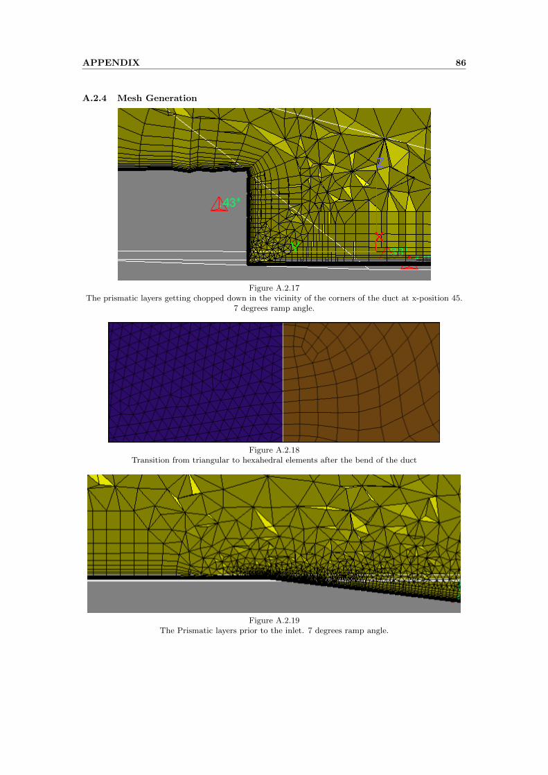
was later removed . . . . . . . . . . . . . . . . . . . . . . . . . . . . . . . . . . . . . . . . . . . . . . . . . . . . . . . . . . . . . . 83A.2.11 Part of the wind tunnel geometry prior to CAD Cleaning . . . . . . . . . . . . . . . . . . . . . . 84A.2.12 Part of the wind tunnel geometry after CAD Cleaning had been performed . . . . . 84A.2.13 -A.2.16 Side view of the air inlet at different ramp angles as seen in CATIA . . . . . . . . . . . . 85A.2.17 The prismatic layers getting chopped down in the vicinity of the corners of the

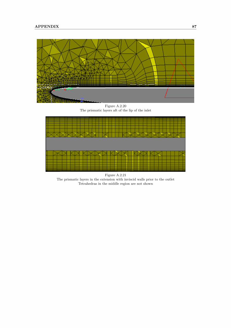
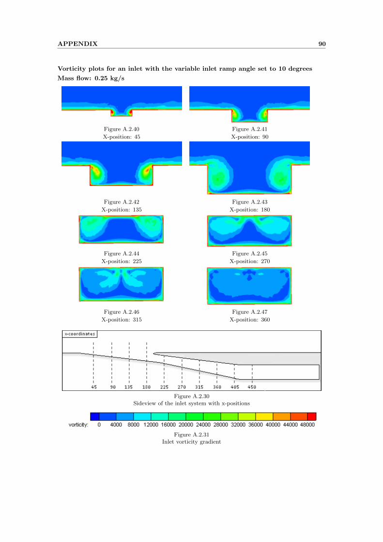
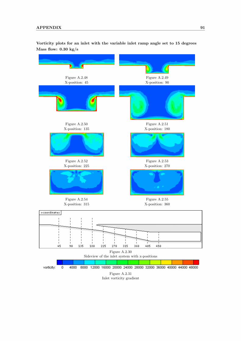
duct at x-position 45. 7 degrees ramp angle. . . . . . . . . . . . . . . . . . . . . . . . . . . . . . . . . . . . 86A.2.18 Transition from triangular to hexahedral elements after the bend of the duct . . . 86A.2.19 The Prismatic layers prior to the inlet. 7 degrees ramp angle . . . . . . . . . . . . . . . . . . . 86A.2.20 The prismatic layers aft of the lip of the inlet . . . . . . . . . . . . . . . . . . . . . . . . . . . . . . . . . . 87A.2.21 The prismatic layers in the extension with inviscid walls prior to the outlet . . . . . 87A.2.22 -A.2.31 Vorticity plots for an inlet with the variable inlet ramp angle set to 4 degrees . . . 88A.2.32 -A.2.39 Vorticity plots for an inlet with the variable inlet ramp angle set to 7 degrees . . . 89A.2.40 -A.2.47 Vorticity plots for an inlet with the variable inlet ramp angle set to 10 degrees . 90A.2.48 -A.2.55 Vorticity plots for an inlet with the variable inlet ramp angle set to 15 degrees . 91A.2.56 -A.2.65 Mach plots for an inlet with the variable inlet ramp angle set to 4 degrees . . . . . . 92A.2.66 -A.2.75 Static pressure plots for an inlet with the variable inlet ramp angle set to

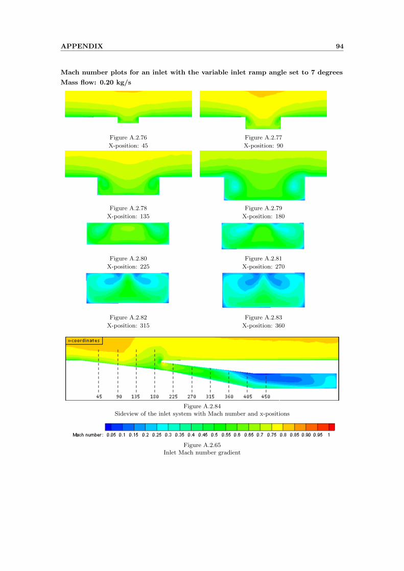
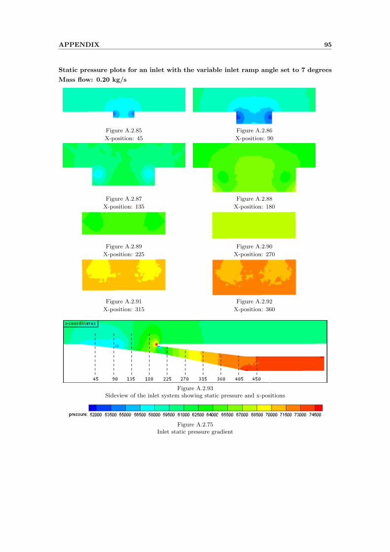
4 degrees . . . . . . . . . . . . . . . . . . . . . . . . . . . . . . . . . . . . . . . . . . . . . . . . . . . . . . . . . . . . . . . . . . . . . . 93A.2.76 -A.2.84 Mach plots for an inlet with the variable inlet ramp angle set to 7 degrees . . . . . . 94A.2.85 -A.2.93 Static pressure plots for an inlet with the variable inlet ramp angle set to

7 degrees . . . . . . . . . . . . . . . . . . . . . . . . . . . . . . . . . . . . . . . . . . . . . . . . . . . . . . . . . . . . . . . . . . . . . . 95

xiv


A.2.94 -A.2.96 Solution span for the last 20 000 iterations. 7 degrees ramp angle.

Mach 0.8. Mass flow: 0.10 kg/s . . . . . . . . . . . . . . . . . . . . . . . . . . . . . . . . . . . . . . . . . . . . . . . . . . 96-97A.2.97 Ram recovery ratio comparison for the 7 degrees ramp angle at different

Mach numbers . . . . . . . . . . . . . . . . . . . . . . . . . . . . . . . . . . . . . . . . . . . . . . . . . . . . . . . . . . . . . . . . . . 97A.2.98 Ram recovery ratio comparison for the 7 degrees ramp angle at different

Mach numbers . . . . . . . . . . . . . . . . . . . . . . . . . . . . . . . . . . . . . . . . . . . . . . . . . . . . . . . . . . . . . . . . . . 98A.2.99 Ram pressure efficiency comparison for different mass flow ratios . . . . . . . . . . . . . . . . . 98A.2.100 Ram pressure efficiency comparison for different Mach numbers . . . . . . . . . . . . . . . . . . 99A.2.101 Drag for the inlet with different ramp angles for different mass flow ratios . . . . . . . . 99A.2.102 Drag for the inlet system with different inlet ramp angles for different

mass flow ratios . . . . . . . . . . . . . . . . . . . . . . . . . . . . . . . . . . . . . . . . . . . . . . . . . . . . . . . . . . . . . . . . . 100A.3.1 The wind tunnel floor prior to the inlet with 35 prismatic layers . . . . . . . . . . . . . . . . . 101A.3.2 The wind tunnel floor prior to the inlet where 31 prismatic layers transitions to

28 prismatic layers . . . . . . . . . . . . . . . . . . . . . . . . . . . . . . . . . . . . . . . . . . . . . . . . . . . . . . . . . . . . . . 101A.3.3 The wind tunnel floor aft of the inlet with 35 prismatic layers . . . . . . . . . . . . . . . . . . . . 101A.3.4 The wind tunnel floor aft of the inlet where 28 prismatic layers transitions to 31

prismatic layers . . . . . . . . . . . . . . . . . . . . . . . . . . . . . . . . . . . . . . . . . . . . . . . . . . . . . . . . . . . . . . . . . 102A.3.5 Side view of the geometrical sources at the wind tunnel test section . . . . . . . . . . . . . . 102A.3.6 The inlet system with coordinate axis . . . . . . . . . . . . . . . . . . . . . . . . . . . . . . . . . . . . . . . . . . . 102A.3.7 Side view of the sources prior to and aft of the inlet . . . . . . . . . . . . . . . . . . . . . . . . . . . . . 104A.3.8 Side view of the prismatic layers in the inlet for the 7 degrees constant ramp angle

configuration as seen in Tecplot 360 . . . . . . . . . . . . . . . . . . . . . . . . . . . . . . . . . . . . . . . . . . . . . 104A.3.9 The iterative process of attaining the prismatic mesh settings inside the inlet . . . . 105A.3.10 The inlet of the wind tunnel geometry. Sources shown in purple . . . . . . . . . . . . . . . . . 106A.3.11 Side view of the prismatic mesh at the bend of the internal duct . . . . . . . . . . . . . . . . . 107A.3.12 Bottom view of the prismatic mesh with no surface refinement in the corners as

seen in Tecplot 360 . . . . . . . . . . . . . . . . . . . . . . . . . . . . . . . . . . . . . . . . . . . . . . . . . . . . . . . . . . . . . . 107A.3.13 Side view of the prismatic mesh at the bend of the internal duct . . . . . . . . . . . . . . . . . 107A.3.14 Bottom view of the prismatic mesh with surface refinement in the corners as

seen in Tecplot 360 . . . . . . . . . . . . . . . . . . . . . . . . . . . . . . . . . . . . . . . . . . . . . . . . . . . . . . . . . . . . . . 108A.3.15 Bottom view of the prismatic mesh with surface refinement in the corners as seen

in Tecplot 360 when generated with the modular meshing feature . . . . . . . . . . . . . . . . 108A.3.16 Mesh comparison when using modular meshing . . . . . . . . . . . . . . . . . . . . . . . . . . . . . . . . . . 109A.5.1 Cross section of the inlet and diffuser section . . . . . . . . . . . . . . . . . . . . . . . . . . . . . . . . . . . . 115

1 Introduction 1

1 Introduction

1.1 Background

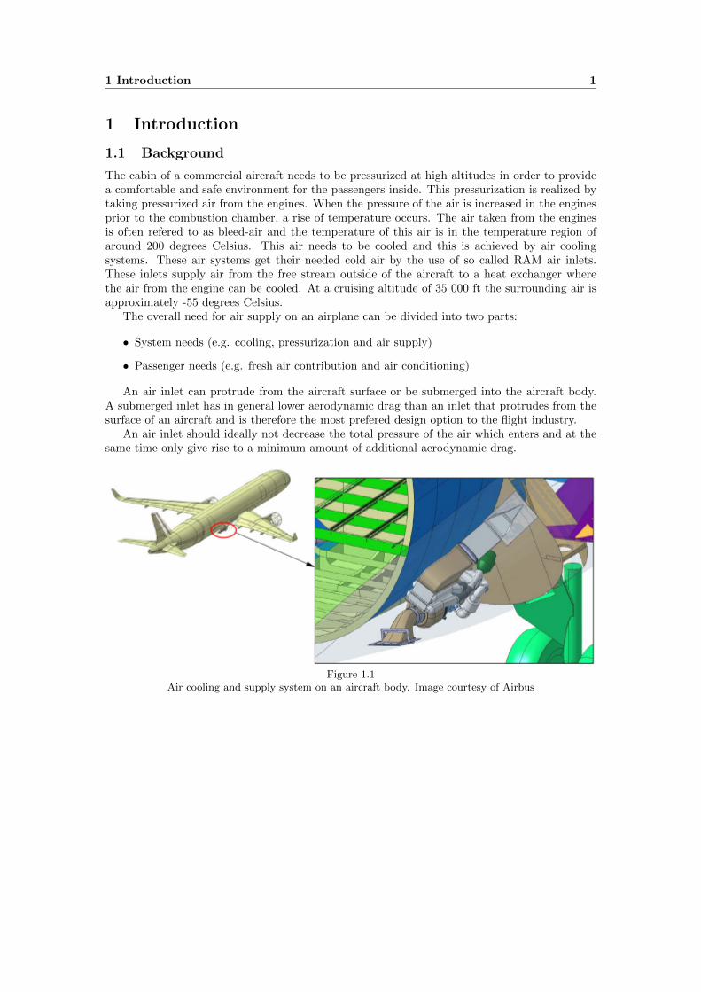
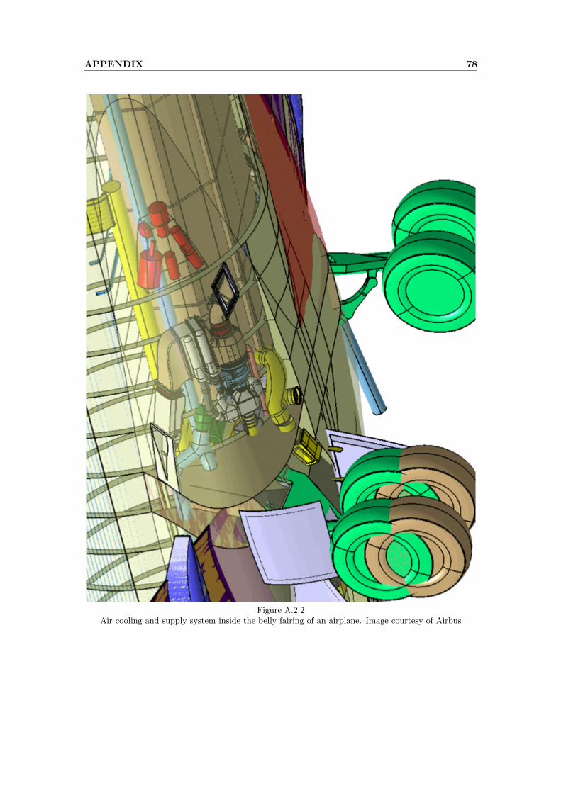
The cabin of a commercial aircraft needs to be pressurized at high altitudes in order to providea comfortable and safe environment for the passengers inside. This pressurization is realized bytaking pressurized air from the engines. When the pressure of the air is increased in the enginesprior to the combustion chamber, a rise of temperature occurs. The air taken from the enginesis often refered to as bleed-air and the temperature of this air is in the temperature region ofaround 200 degrees Celsius. This air needs to be cooled and this is achieved by air coolingsystems. These air systems get their needed cold air by the use of so called RAM air inlets.These inlets supply air from the free stream outside of the aircraft to a heat exchanger wherethe air from the engine can be cooled. At a cruising altitude of 35 000 ft the surrounding air isapproximately -55 degrees Celsius.

The overall need for air supply on an airplane can be divided into two parts:

• System needs (e.g. cooling, pressurization and air supply)

• Passenger needs (e.g. fresh air contribution and air conditioning)

An air inlet can protrude from the aircraft surface or be submerged into the aircraft body.A submerged inlet has in general lower aerodynamic drag than an inlet that protrudes from thesurface of an aircraft and is therefore the most prefered design option to the flight industry.

An air inlet should ideally not decrease the total pressure of the air which enters and at thesame time only give rise to a minimum amount of additional aerodynamic drag.

Figure 1.1Air cooling and supply system on an aircraft body. Image courtesy of Airbus

1.1 Background 2

1.1.1 Project ECOcents

Figure 1.2ECOCENTS Logo

This thesis contributes with its results to the government-funded project ECOCENTS. ECO-CENTS stands for ”Effizientes Cooling Center fur Flugzeugsysteme” which translates intoEnglish as ”Efficient Cooling Center for Aircraft Systems”.

This project consist of two main research topics:

• Cooling center

• Cooling channel

Cooling center deals with the design of heat exchanges while Cooling channel deals with theinlet, outlet and channel design. Previous studies have been made on the design of the air inletin connection to this project. The investigation carried out in this thesis is however the firstdetailed investigation of wind tunnel simulations in combination with air systems inlets usingthe RANS flow solver TAU developed by the German Aerospace Center (DLR).

1.2 Purpose 3

1.2 Purpose

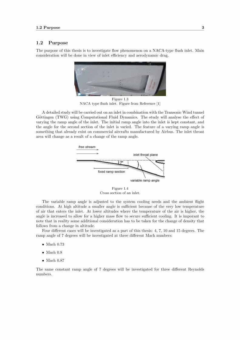
The purpose of this thesis is to investigate flow phenomenon on a NACA-type flush inlet. Mainconsideration will be done in view of inlet efficiency and aerodynamic drag.

Figure 1.3NACA type flush inlet. Figure from Reference [1]

A detailed study will be carried out on an inlet in combination with the Transonic Wind tunnelGottingen (TWG) using Computational Fluid Dynamics. The study will analyse the effect ofvarying the ramp angle of the inlet. The initial ramp angle into the inlet is kept constant, andthe angle for the second section of the inlet is varied. The feature of a varying ramp angle issomething that already exist on commercial aircrafts manufactured by Airbus. The inlet throatarea will change as a result of a change of the ramp angle.

Figure 1.4Cross section of an inlet.

The variable ramp angle is adjusted to the system cooling needs and the ambient flightconditions. At high altitude a smaller angle is sufficient because of the very low temperatureof air that enters the inlet. At lower altitudes where the temperature of the air is higher, theangle is increased to allow for a higher mass flow to secure sufficient cooling. It is imporant tonote that in reality some additional consideration has to be taken for the change of density thatfollows from a change in altitude.

Four different cases will be investigated as a part of this thesis: 4, 7, 10 and 15 degrees. Theramp angle of 7 degrees will be investigated at three different Mach numbers:

• Mach 0.73

• Mach 0.8

• Mach 0.87

The same constant ramp angle of 7 degrees will be investigated for three different Reynoldsnumbers.

1.2 Purpose 4

• Reynolds number: 5·106



The three other angles will be investigated at a Reynolds number of 10·106 and Mach 0.8. Acomparison of the results obtained CFD results will be made with an empirical method analysis.Suggestions will be given for optimal arrangements of air inlets with regards to caused floweffects. The CFD investigation will be used to validate and support a wind tunnel campaign inTWG (DLR Gottingen) that is planned for October 2011.

1.3 Scope of work 5

1.3 Scope of work

• Study of literature relevant to the topic of the thesis. This includes presentations, booksand technical reports on Computational Fluid Dynamics and Air Inlets.

• Familiarization with the tools necessary to achieve the objective (CATIA, CENTAUR,TAU, Tau BL and Tecplot 360).

• Prepare the wind tunnel CAD geometry for the data export into the meshing software.

• Prepare a number of CAD models for the purpose of investigating different NACA air inletramp angles.

• Generate several computational grids.

• Setup of TAU boundary conditions and execute TAU calculations.

• Detailed analysis of the results.

• Give suggestions for optimal air inlet ramp angles.

• Make recommendations for future work.

• Write a thesis paper for the Degree of Bachelor of Science in Engineering.

• Hold a presentation in English on the results obtained for interested parties at Airbus sitein Bremen, Germany.

• Hold a presentation in Swedish on the scope of this thesis and the results obtained atMalardalen University in Vasteras, Sweden.

1.3 Scope of work 6

2 Theory 7

2 Theory

2.1 Boundary Layer Theory

When studying air flow over a solid body it is appropriate to divide the analysis of the flow intotwo parts. Close to the surface of the solid body friction forces play an important part whereasfurther out into the free stream friction forces can be neglected. The idea is to treat the air flowclose to a surface seperately. This concept was first suggested in 1904 by a man named LudwigPrandtl.

Due to the friction between the surface and the moving gas, the air flow closest to the surfacewill tend to adhere. This phenomenon is known as the no-slip condition. This is true for allfluids but for the purpose of this thesis we are mainly interested in the medium air. The velocitygradually increases further away from the surface and eventually reaches the free stream velocity,denoted as V2 in Figure 2.1.

Figure 2.1Velocity profile through a boundary layer. Figure from Reference [2]

The region in which this velocity gradient exist is called the boundary layer. The velocityreduction of the flow inside the boundary layer gives rise to shear friction τw on the surface ofthe solid body. This shear friction is the source of a form of drag called skin friction drag.

The thickness of the boundary layer, denoted as δ, is defined as the distance normal to thesurface up to a point where the flow has reached 99% of the free stream velocity. Due to theeffects of friction, the thickness of the boundary layer increases as the flow moves a distance overthe surface and can attain a considerable thickness, e.g, at the end of a flat plate (Figure 2.2) orat the fuselage tail of an aircraft.

Figure 2.2Boundary layer growth along a flat plate. Figure from Reference [2]

The boundary layer thickness is an important parameter to consider when placing an air inlet ona surface as this low-velocity, low energy boundary layer decreases the performance of the inlet.

2.2 Drag 8

2.2 Drag

Aerodynamic drag is the force acting parallel to the free stream on a body immersed in a movingfluid. All forces in aerodynamics have their origin in pressure distribution and shear stressdistribution over the body surface. It is hence appropriate to divide the drag of a body into twocategories, pressure drag and skin friction drag, depending on which one of these sources it hasits physical origin. There are additional types of aerodynamic drag which play an importantrole at the overall aerodynamics of aircrafts: interference drag, lift-induced drag and wave drag.For aerodynamic design of air systems they might not be completely negligible but will not beregarded here in detail.

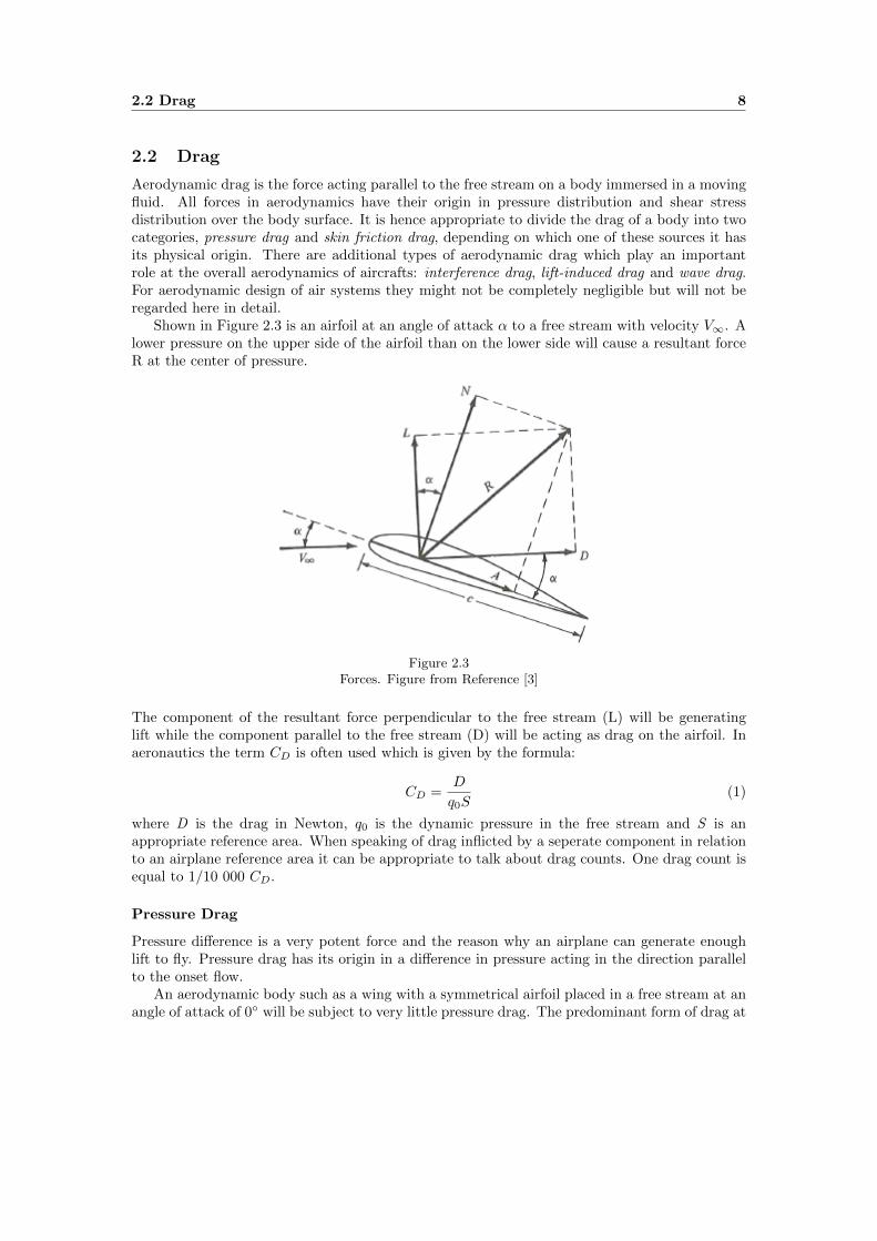
Shown in Figure 2.3 is an airfoil at an angle of attack α to a free stream with velocity V∞. Alower pressure on the upper side of the airfoil than on the lower side will cause a resultant forceR at the center of pressure.

Figure 2.3Forces. Figure from Reference [3]

The component of the resultant force perpendicular to the free stream (L) will be generatinglift while the component parallel to the free stream (D) will be acting as drag on the airfoil. Inaeronautics the term CD is often used which is given by the formula:

CD =D

q0S(1)

where D is the drag in Newton, q0 is the dynamic pressure in the free stream and S is anappropriate reference area. When speaking of drag inflicted by a seperate component in relationto an airplane reference area it can be appropriate to talk about drag counts. One drag count isequal to 1/10 000 CD.

Pressure Drag

Pressure difference is a very potent force and the reason why an airplane can generate enoughlift to fly. Pressure drag has its origin in a difference in pressure acting in the direction parallelto the onset flow.

An aerodynamic body such as a wing with a symmetrical airfoil placed in a free stream at anangle of attack of 0◦ will be subject to very little pressure drag. The predominant form of drag at

2.3 Flight Mechanics 9

this angle of attack would be skin friction drag, but as α is increased to a certain degree the flowwill eventually separate at the trailing edge of the wing. The separation point will move furtherforward on the upper side of the wing with an increasing angle of attack. Flow separation altersthe pressure distribution over the wing, lowering the pressure at the trailing edge and increasingthe pressure at the leading edge resulting in a large increase in pressure drag.

Skin Friction Drag

The skin friction drag is due to viscous effects on the surface of a body due to the presence ofthe boundary layer. The closer the flow gets to the surface, the more the motion of the flowis retarded by friction. An equal force in the opposite direction affects the surface of the solidbody; this force is the skin friction drag. A larger surface area will give rise to a higher valueof skin friction drag. A term used in the aircraft industry is wetted area which is the area incontact with the moving fluid and is often used as a reference area for skin friction drag.

2.3 Flight Mechanics

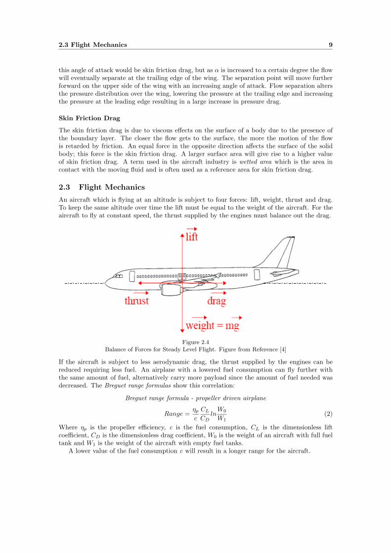
An aircraft which is flying at an altitude is subject to four forces: lift, weight, thrust and drag.To keep the same altitude over time the lift must be equal to the weight of the aircraft. For theaircraft to fly at constant speed, the thrust supplied by the engines must balance out the drag.

Figure 2.4Balance of Forces for Steady Level Flight. Figure from Reference [4]

If the aircraft is subject to less aerodynamic drag, the thrust supplied by the engines can bereduced requiring less fuel. An airplane with a lowered fuel consumption can fly further withthe same amount of fuel, alternatively carry more payload since the amount of fuel needed wasdecreased. The Breguet range formulas show this correlation:

Breguet range formula - propeller driven airplane

Range =ηpc

CLCD

lnW0

W1(2)

Where ηp is the propeller efficiency, c is the fuel consumption, CL is the dimensionless liftcoefficient, CD is the dimensionless drag coefficient, W0 is the weight of an aircraft with full fueltank and W1 is the weight of the aircraft with empty fuel tanks.

A lower value of the fuel consumption c will result in a longer range for the aircraft.

2.4 Ram Pressure Efficiency 10

Breguet range formula - jet airplane

Range = 2

√2

ρ0S

1

ct

CLCD

(W0 −W1) (3)

Where ρ0 is the density of the air in the free stream, S is the wing area and ct is the thrust-specificfuel consumption.

A lower value of the thrust-specific fuel consumption ct will also here result in a longer rangefor the aircraft.

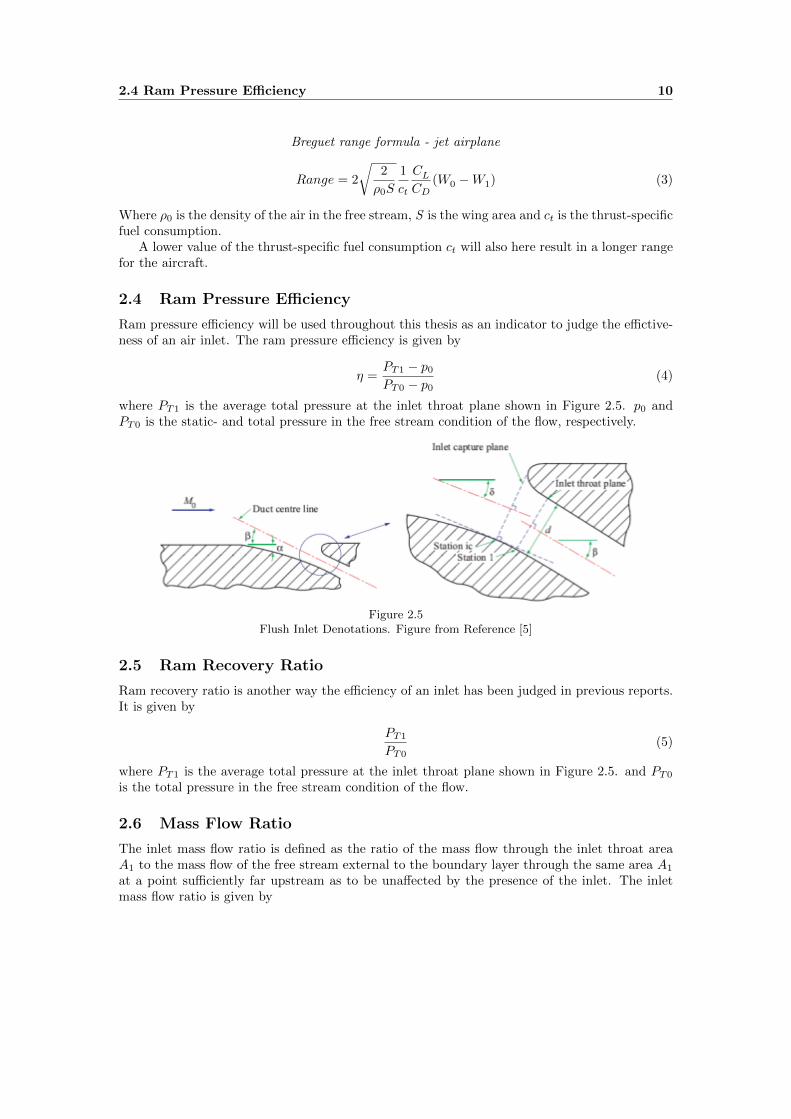
2.4 Ram Pressure Efficiency

Ram pressure efficiency will be used throughout this thesis as an indicator to judge the effictive-ness of an air inlet. The ram pressure efficiency is given by

η =PT1 − p0PT0 − p0

(4)

where PT1 is the average total pressure at the inlet throat plane shown in Figure 2.5. p0 andPT0 is the static- and total pressure in the free stream condition of the flow, respectively.

Figure 2.5Flush Inlet Denotations. Figure from Reference [5]

2.5 Ram Recovery Ratio

Ram recovery ratio is another way the efficiency of an inlet has been judged in previous reports.It is given by

PT1

PT0(5)

where PT1 is the average total pressure at the inlet throat plane shown in Figure 2.5. and PT0

is the total pressure in the free stream condition of the flow.

2.6 Mass Flow Ratio

The inlet mass flow ratio is defined as the ratio of the mass flow through the inlet throat areaA1 to the mass flow of the free stream external to the boundary layer through the same area A1

at a point sufficiently far upstream as to be unaffected by the presence of the inlet. The inletmass flow ratio is given by

2.7 Navier-Stokes Equations 11

m1

m0=ρ1 · V1 ·A1

ρ0 · V0 ·A1=ρ1 · V1ρ0 · V0

(6)

where ρ is the density, V is the flow velocity and A1 is the inlet throat area. Subscript 1 indicatesvalues measured at the inlet throat plane (see Figure 1.4 and Figure 2.5) and subscript 0 denotesfree stream values.

The value of the mass flow ratio is closely related to the drag of an inlet. The drag increaseswith increasing mass flow ratio [6].

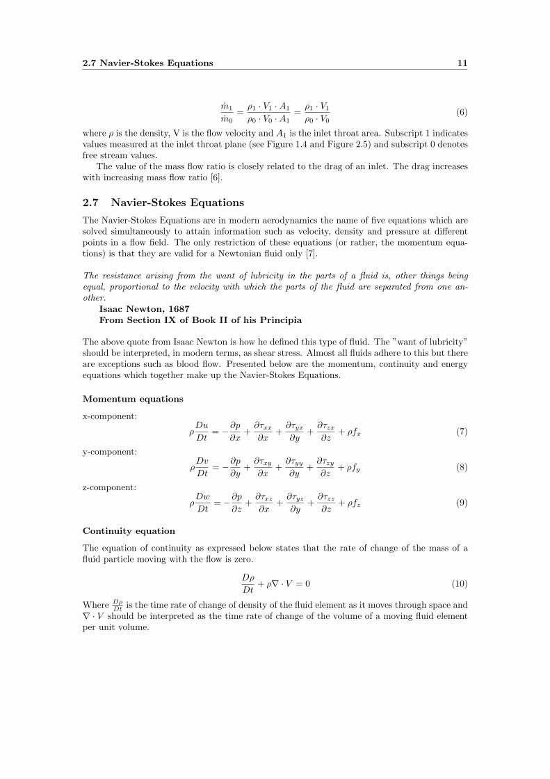
2.7 Navier-Stokes Equations

The Navier-Stokes Equations are in modern aerodynamics the name of five equations which aresolved simultaneously to attain information such as velocity, density and pressure at differentpoints in a flow field. The only restriction of these equations (or rather, the momentum equa-tions) is that they are valid for a Newtonian fluid only [7].

The resistance arising from the want of lubricity in the parts of a fluid is, other things beingequal, proportional to the velocity with which the parts of the fluid are separated from one an-other.

Isaac Newton, 1687From Section IX of Book II of his Principia

The above quote from Isaac Newton is how he defined this type of fluid. The ”want of lubricity”should be interpreted, in modern terms, as shear stress. Almost all fluids adhere to this but thereare exceptions such as blood flow. Presented below are the momentum, continuity and energyequations which together make up the Navier-Stokes Equations.

Momentum equations

x-component:

ρDu

Dt= −∂p

∂x+∂τxx∂x

+∂τyx∂y

+∂τzx∂z

+ ρfx (7)

y-component:

ρDv

Dt= −∂p

∂y+∂τxy∂x

+∂τyy∂y

+∂τzy∂z

+ ρfy (8)

z-component:

ρDw

Dt= −∂p

∂z+∂τxz∂x

+∂τyz∂y

+∂τzz∂z

+ ρfz (9)

Continuity equation

The equation of continuity as expressed below states that the rate of change of the mass of afluid particle moving with the flow is zero.

Dρ

Dt+ ρ∇ · V = 0 (10)

Where DρDt is the time rate of change of density of the fluid element as it moves through space and

∇ · V should be interpreted as the time rate of change of the volume of a moving fluid elementper unit volume.

2.8 Reynolds-Averaged Navier-Stokes Equations 12

Energy equation

ρD

Dt

(e+

V 2

2

)= pq +

∂

∂x

(k∂T

∂x

)+

∂

∂y

(k∂T

∂y

)+

∂

∂z

(k∂T

∂z

)− ∂(up)

∂x− ∂(vp)

∂y−

−∂(wp)

∂z+∂(uτxx)

∂x+∂(uτyx)

∂y+∂(uτzx)

∂z+∂(vτxy)

∂x+∂(vτyy)

∂y+∂(vτzy)

∂z+

+∂(wτxz)

∂x+∂(wτyz)

∂y+∂(wτzz)

∂z+ ρf · V

(11)

Where ρ is the local density, p is the local pressure, e is the internal energy due to randommolecular motion and u, v, w are the velocities in the x, y, z-directions respectively. Theseequations were here presented in non-conservation form. For a detailed derivation of theseequations and an explanation of the difference between conservation and non-conservation formthe reader is referred to Reference [7].

When examining the Navier Stokes equations, one thing we can note is that we have fiveequations and six unknown flow field variables, namely: ρ, p, u, v, w and e. To solve a systemwhich consists of multiple equations the number of equations should be equal to the number ofvariables. To resolve this we add a sixth equation to the system, the equation of state for aperfect gas

p = ρ ·R · T (12)

where R is the specific gas constant. This, however, gives us a seventh unknown variable,the temperature T. A thermodynamic relation between state variables is necessary to close thesystem. For a calorically perfect gas (constant specific heats) we can use the equation

e = cv · T (13)

where cv is the specific heat at a constant volume. This equation is sometimes referred to as thecaloric equation of state.

2.8 Reynolds-Averaged Navier-Stokes Equations

The Navier-Stokes equations contain the physical relations needed to describe a turbulent flowfor a Newtonian fluid. However, solving these equations for a turbulent flow would require anenormous amount of computational power and time. To manage this problem averaging con-cepts introduced by Osborn Reynolds in 1895 are used. Reynolds averaging can be expressed ina number of different forms. The three most commonly used forms [8] are:

Time average

FT (x) = limx→∞

1

T

∫ t+T

t

f(x, t)dt (14)

The spatial average

FV (t) = limV→∞

1

V

∫ ∫ ∫V

f(x, t)dV (15)

Ensemble average

FE(x, t) = limN→∞

1

N

N∑n=1

fn(x, t)dV (16)

2.9 Spatial Discretisation 13

The time average form is used to calculate the properties of stationary flows, that is, flows thatdo not vary with time. An example of a flow of this type is given in Reference [8] as flow insidea pipe driven by a constant-speed blower. This form is the most commonly used as most flowsin engineering are of this nature. The spatial average can be used to describe turbulence whichis on average uniform in all directions while the ensemble average is appropriate for flows thatdecay with time.

An unfortunate consequence of applying Reynolds-Averaging of the Navier-Stokes equationsis the introduction of six new unknown variables known as the Reynolds-stress components. Thenew variables have to be found with the help of turbulence models. Different turbulence modelshave been introduced since the time of Reynolds solving approach.

The RANS solver TAU used in this thesis was established and is still being developed bythe German Aerospace Center (DLR). The following turbulence one- and two equation eddy-viscosity models are implemented in TAU:

• One-equation eddy-viscosity models

- SAO-model (Spalart-Allmaras, original version)

- SAE-model (Spalart-Allmaras, Edwards modification)

- SAM-model (Spalart-Allmaras, modified version)

- SALSA-model (Strain Adaptive Linear SA-model)

• Two-equation eddy-viscosity models

- Wilcox k-ω model

- Menter Baseline model

- Menter SST model

- LEA k-ω model

- NLR TNT Model

- Wilcox k-ω model + SST

- Menter 2layer k-ε model

Additional models does exist for modeling the effects of turbulent flows in TAU. For a completelist and an in-depth explanation of the different turbulence models, the reader is referred toReference [9] and Reference [10]. The turbulence model used for the CFD calculations in thisthesis is the Spalart-Allmaras, Edwards modification model.

2.9 Spatial Discretisation

The spatial discretisation of the Navier-stokes equations, i.e., the numerical approximation of theviscous and convective fluxes as well as the source term, can be done by three main approaches:the finite difference method, the finite element method and the finite volume method. The RANSsolver TAU used in this thesis is based on the finite volume method [11]. To apply any of thesemethods a computational grid is needed. Three types of grids are used in CFD: structured grids,unstructured grids and hybrid grids.


2.9.1 Computational Grids

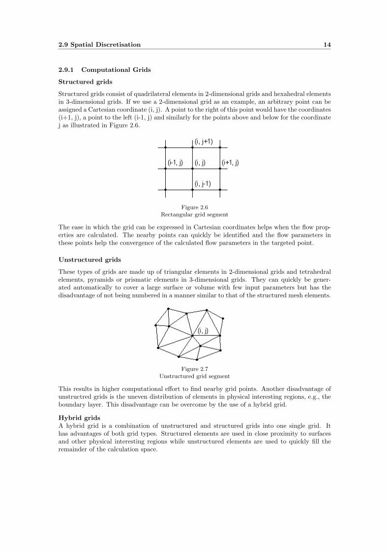
Structured grids

Structured grids consist of quadrilateral elements in 2-dimensional grids and hexahedral elementsin 3-dimensional grids. If we use a 2-dimensional grid as an example, an arbitrary point can beassigned a Cartesian coordinate (i, j). A point to the right of this point would have the coordinates(i+1, j), a point to the left (i-1, j) and similarly for the points above and below for the coordinatej as illustrated in Figure 2.6.

Figure 2.6Rectangular grid segment

The ease in which the grid can be expressed in Cartesian coordinates helps when the flow prop-erties are calculated. The nearby points can quickly be identified and the flow parameters inthese points help the convergence of the calculated flow parameters in the targeted point.

Unstructured grids

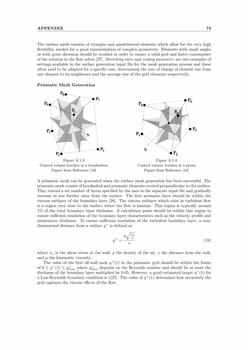
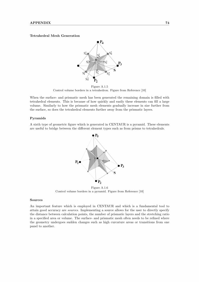
These types of grids are made up of triangular elements in 2-dimensional grids and tetrahedralelements, pyramids or prismatic elements in 3-dimensional grids. They can quickly be gener-ated automatically to cover a large surface or volume with few input parameters but has thedisadvantage of not being numbered in a manner similar to that of the structured mesh elements.

Figure 2.7Unstructured grid segment

This results in higher computational effort to find nearby grid points. Another disadvantage ofunstructred grids is the uneven distribution of elements in physical interesting regions, e.g., theboundary layer. This disadvantage can be overcome by the use of a hybrid grid.

Hybrid gridsA hybrid grid is a combination of unstructured and structured grids into one single grid. Ithas advantages of both grid types. Structured elements are used in close proximity to surfacesand other physical interesting regions while unstructured elements are used to quickly fill theremainder of the calculation space.


2.9.2 Discretisation Methods

Finite Difference Method

This method is directly applied to the differential form of the governing Navier-Stokes equations.It employs a Taylor series expansion of the derivatives of the flow variables [9]. It has theadvantage of simplicity but requires a structured grid to work with. The use of the finite differencemethod is very limited in modern aerodynamics.

Finite Element Method

The finite element method when applied to the Navier-Stokes equations starts with a subdivisionof the physical space into triangular elements when working with a 2-dimensional grid, and intotetrahedral elements when working with 3-dimensions. The finite element method requires thegoverning equations to be expressed in integral form, and thus the equations have to be trans-formed from differential form. This method is advantageous for use around complex geometriesbecause of its unstructured approach and the mentioned use of the integral form of the governingequations [9]. The finite element method is commonly used in structural analysis of materials.

Finite Volume Method

The finite volume method requires the physical space to be divided into a number of polyhedralcontrol volumes in order to discretise the governing equations. The finite volume method requiresalso, as in the case with the finite element method, the integral form of the Navier-Stokesequations. The advantage of this method is that the discretisation is carried out directly in thephysical space, requiring no transformation between the physical space and a calculation grid.The method can be applied to both structured and unstructured grids.

2.9.3 Central and Upwind Schemes

The methods discussed above require a numerical scheme to perform the spatial discretisation.While numerous different schemes exist, a brief explanation will only here be given for the centralscheme and the upwind scheme as they are employed by the flow solver TAU [11].

Central Schemes

Belonging to this group are schemes based on central averaging or central difference formula.The values of the variables on either side of an element are averaged to evaluate the fluctuationsin close proximity to the element. However, central schemes require an artificial dissipation tokeep stable. A clear advantage is that in most cases a central scheme is more effective than theupwind scheme in view of CPU usage.

Upwind Schemes

Upwind schemes are able to capture discontinuities more accurately than central schemes andsolve boundary layer parameters accurately with fewer calculation points. The downside ofupwind schemes is that limiters have to be used to prevent oscillations of the solution variablesclose to strong discontinuities.

The central and upwind scheme can be combined when making a complete calculation of a flowfield to obtain a converged and accurate solution. When using the flow solver TAU it has proven

2.10 Time Discretisation 16

advantagous to use upwind scheme for the first thousand or more calculations, and then switchto a central scheme for the remainder of the calculations.

2.10 Time Discretisation

For greater flexibility different approaches are used for spatial and time discretisation. Twodifferent types of schemes are employed by TAU for time discretisation of the governing equations,namely explicit- and implicit schemes [10].

Explicit Schemes

In the explicit approach to the governing equations there is only one unknown variable. Let thisvariable be denoted by Ani where i denote the node we are investigating, and n indicates themoment in time. Known values An−1i−1 , A

n−1i and An−1i+1 from the previous time-step are used to

calculate the flow parameters in the new point. One equation and one unknown results in aneasy definition and set-up of the problem. Very advantageous from a programming point of viewbut it does have its drawbacks. In some cases the time-step has to be very small to maintainstability of the solution which can result in long calculation times. The use of parallel processorshas made these type schemes very interesting as each processor can work on a separate part ofthe grid with minimum intercommunication necessary [7].

Implicit Schemes

Implicit schemes are much more complicated to solve than the explicit schemes. Instead of anequation with the unknown variable at one point Ani requiring information from points in theprevious time-step, we have an equation with three unknowns, namely Ani−1, A

ni and Ani+1. The

solution must be attained by solving an entire system of equations simultaneously. This approachhas the advantage of allowing for greater time-steps than the explicit schemes resulting in lesscomputational time. It should however be kept in mind that due to the system of equations beingmore complex, each time-step takes longer to calculate. As this method requires large amountsof information to be exchanged between nodes it is less suited for parallel processors [7].

3 Methodology 17

3 Methodology

3.1 Preliminary Studies

3.1.1 Inlets

There are two basic types of inlets: scoop inlets protruding from a surface into the free streamand flush inlets submerged into a body.

Figure 3.1Scoop inlet. Figure from Reference [6]

Figure 3.2Flush inlet. Figure from Reference [6]

Advantages and disadvantages exist with both design choices. While the scoop inlet has theadvantage of avoiding the low energy boundary layer which reduces the efficiency of an airinlet, it has typically the disadvantage of a greater increase of aerodynamic drag compared to asubmerged inlet.

The aircraft industry is very interested in solutions that reduce the aerodynamic drag, andin extent the fuel consumption of an airplane. The air inlet investigated in this report is of flushtype.

3.1.2 Flush Inlets

An air inlet should not, if optimal, increase the drag of the body into which it is placed or reducethe energy available in the air which enters the inlet. These critera cannot be fully met by any

3.1 Preliminary Studies 18

air inlet, but design parameters can be changed to come close to an optimum for a specific flightcondition. For low drag it is advantagous to use a flushed inlet which is submerged into thesurface of the body into which it is placed. The flush type is also advantagous to avoid foreignobject damage on the inlet.

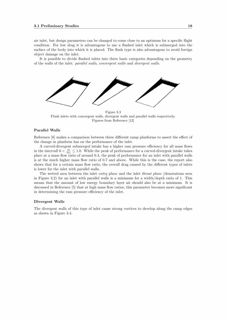
It is possible to divide flushed inlets into three basic categories depending on the geometryof the walls of the inlet: parallel walls, convergent walls and divergent walls.

Figure 3.3Flush inlets with convergent walls, divergent walls and parallel walls respectively.

Figures from Reference [12]

Parallel Walls

Reference [6] makes a comparison between three different ramp planforms to assert the effect ofthe change in planform has on the performance of the inlet.

A curved-divergent submerged intake has a higher ram pressure efficiency for all mass flowsin the intervall 0 < m

m0≤ 1.0. While the peak of performance for a curved-divergent intake takes

place at a mass flow ratio of around 0.4, the peak of performance for an inlet with parallel wallsis at the much higher mass flow ratio of 0.7 and above. While this is the case, the report alsoshows that for a certain mass flow ratio, the overall drag caused by the different types of inletsis lower for the inlet with parallel walls.

The wetted area between the inlet entry plane and the inlet throat plane (denotations seenin Figure 3.2) for an inlet with parallel walls is a minimum for a width/depth ratio of 1. Thismeans that the amount of low energy boundary layer air should also be at a minimum. It isdiscussed in Reference [5] that at high mass flow ratios, this parameter becomes more significantin determining the ram pressure efficiency of the inlet.

Divergent Walls

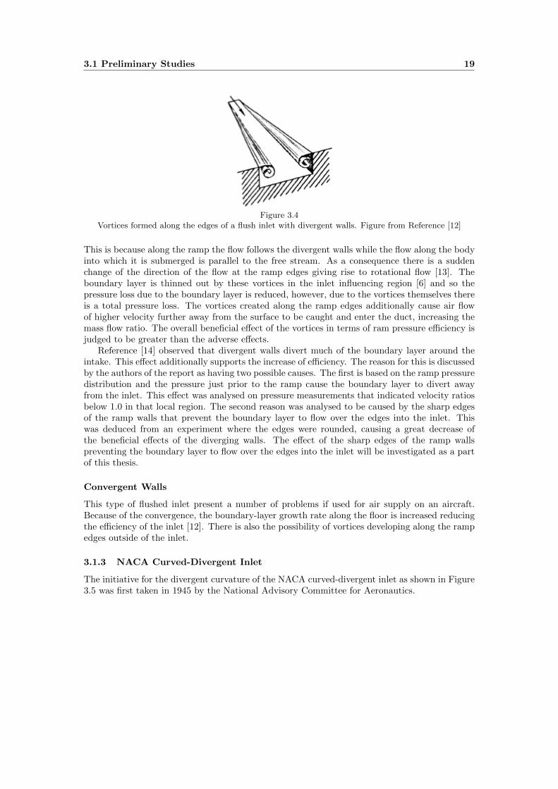
The divergent walls of this type of inlet cause strong vortices to develop along the ramp edgesas shown in Figure 3.4.


Figure 3.4Vortices formed along the edges of a flush inlet with divergent walls. Figure from Reference [12]

This is because along the ramp the flow follows the divergent walls while the flow along the bodyinto which it is submerged is parallel to the free stream. As a consequence there is a suddenchange of the direction of the flow at the ramp edges giving rise to rotational flow [13]. Theboundary layer is thinned out by these vortices in the inlet influencing region [6] and so thepressure loss due to the boundary layer is reduced, however, due to the vortices themselves thereis a total pressure loss. The vortices created along the ramp edges additionally cause air flowof higher velocity further away from the surface to be caught and enter the duct, increasing themass flow ratio. The overall beneficial effect of the vortices in terms of ram pressure efficiency isjudged to be greater than the adverse effects.

Reference [14] observed that divergent walls divert much of the boundary layer around theintake. This effect additionally supports the increase of efficiency. The reason for this is discussedby the authors of the report as having two possible causes. The first is based on the ramp pressuredistribution and the pressure just prior to the ramp cause the boundary layer to divert awayfrom the inlet. This effect was analysed on pressure measurements that indicated velocity ratiosbelow 1.0 in that local region. The second reason was analysed to be caused by the sharp edgesof the ramp walls that prevent the boundary layer to flow over the edges into the inlet. Thiswas deduced from an experiment where the edges were rounded, causing a great decrease ofthe beneficial effects of the diverging walls. The effect of the sharp edges of the ramp wallspreventing the boundary layer to flow over the edges into the inlet will be investigated as a partof this thesis.

Convergent Walls

This type of flushed inlet present a number of problems if used for air supply on an aircraft.Because of the convergence, the boundary-layer growth rate along the floor is increased reducingthe efficiency of the inlet [12]. There is also the possibility of vortices developing along the rampedges outside of the inlet.

3.1.3 NACA Curved-Divergent Inlet

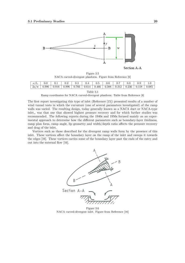
The initiative for the divergent curvature of the NACA curved-divergent inlet as shown in Figure3.5 was first taken in 1945 by the National Advisory Committee for Aeronautics.


Figure 3.5NACA curved-divergent planform. Figure from Reference [6]

x/lr 0.0 0.1 0.2 0.3 0.4 0.5 0.6 0.7 0.8 0.9 1.0

2z/w 0.996 0.916 0.996 0.766 0.614 0.466 0.388 0.312 0.236 0.158 0.085

Table 3.1Ramp coordinates for NACA curved-divergent planform. Table from Reference [6]

The first report investigating this type of inlet (Reference [15]) presented results of a number ofwind tunnel tests in which the curvature (one of several parameters investigated) of the rampwalls was varied. The resulting design, today generally known as a NACA duct or NACA-typeinlet,, was that one that showed highest pressure recovery and for which further studies wasrecommended. The following reports during the 1940s and 1950s focused mainly on an exper-imental approach to determine how the different parameters such as boundary-layer thickness,ramp plan form, ramp angle, lip geometry and width/depth ratio affects the pressure recoveryand drag of the inlet.

Vortices such as those described for the divergent ramp walls form by the presence of thisinlet. These vortices affect the boundary layer on the ramp of the inlet and sweeps it towardsthe edges [16]. These vortices carries some of the boundary layer past the ends of the entry andout into the external flow [16].

Figure 3.6NACA curved-divergent inlet. Figure from Reference [16]


3.1.4 Design Parameters

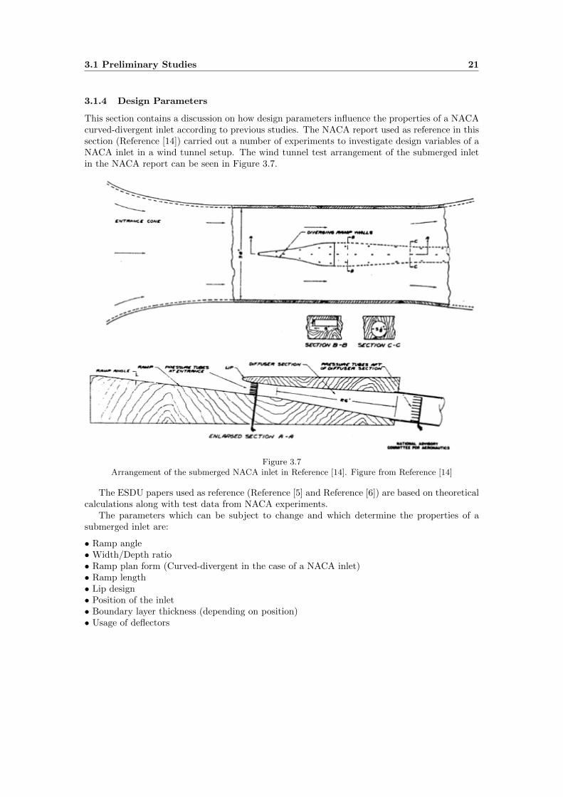
This section contains a discussion on how design parameters influence the properties of a NACAcurved-divergent inlet according to previous studies. The NACA report used as reference in thissection (Reference [14]) carried out a number of experiments to investigate design variables of aNACA inlet in a wind tunnel setup. The wind tunnel test arrangement of the submerged inletin the NACA report can be seen in Figure 3.7.

Figure 3.7Arrangement of the submerged NACA inlet in Reference [14]. Figure from Reference [14]

The ESDU papers used as reference (Reference [5] and Reference [6]) are based on theoreticalcalculations along with test data from NACA experiments.

The parameters which can be subject to change and which determine the properties of asubmerged inlet are:

• Ramp angle• Width/Depth ratio• Ramp plan form (Curved-divergent in the case of a NACA inlet)• Ramp length• Lip design• Position of the inlet• Boundary layer thickness (depending on position)• Usage of deflectors


Ramp Angle

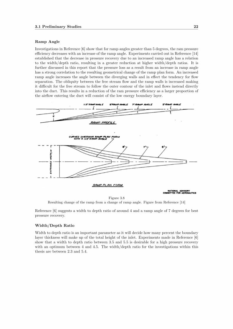
Investigations in Reference [6] show that for ramp angles greater than 5 degrees, the ram pressureefficiency decreases with an increase of the ramp angle. Experiments carried out in Reference [14]established that the decrease in pressure recovery due to an increased ramp angle has a relationto the width/depth ratio, resulting in a greater reduction at higher width/depth ratios. It isfurther discussed in this report that the pressure loss as a result from an increase in ramp anglehas a strong correlation to the resulting geometrical change of the ramp plan form. An increasedramp angle increases the angle between the diverging walls and in effect the tendency for flowseparation. The obliquity between the free stream flow and the ramp walls is increased makingit difficult for the free stream to follow the outer contour of the inlet and flows instead directlyinto the duct. This results in a reduction of the ram pressure efficiency as a larger proportion ofthe airflow entering the duct will consist of the low energy boundary layer.

Figure 3.8Resulting change of the ramp from a change of ramp angle. Figure from Reference [14]

Reference [6] suggests a width to depth ratio of around 4 and a ramp angle of 7 degrees for bestpressure recovery.

Width/Depth Ratio

Width to depth ratio is an important parameter as it will decide how many percent the boundarylayer thickness will make up of the total height of the inlet. Experiments made in Reference [6]show that a width to depth ratio between 3.5 and 5.5 is desirable for a high pressure recoverywith an optimum between 4 and 4.5. The width/depth ratio for the investigations within thisthesis are between 2.3 and 5.4.


Ramp Length

This parameters is directly related to the ramp angle and the width/depth ratio. It is in practicalapplications usually the parameter that place restrictions on the geometry of the inlet.

Boundary Layer Thickness

The boundary layer thickness has been proven to play an important role for the ram pressureefficiency of an inlet. An increase in boundary layer thickness causes a decrease of the rampressure efficiency [5]. This could be expected as the boundary layer contains flow at a lowervelocity than that of the free stream. A general recommendation to avoid a thick boundary layerentering the inlet is to place the inlet closer to the leading edge of the surface into which it issubmerged.

The boundary layer on the ramp walls of the air inlet has no initial thickness and grows overa very short distance before entering the inlet and has thus only a small impact on the rampressure efficiency. The reduction of ram pressure efficiency due to the boundary layer from thewalls of the inlet is only about 5-10 % of that due to the boundary layer on the ramp [12].

Position of the Inlet

The main need for air supply on larger modern commercial aircrafts is usually supplied by ramair inlets on the belly fairing. The heat exchanger and related ducting are found inside the bellyfairing, whwich is the fairing between aircraft wing and fuselage.

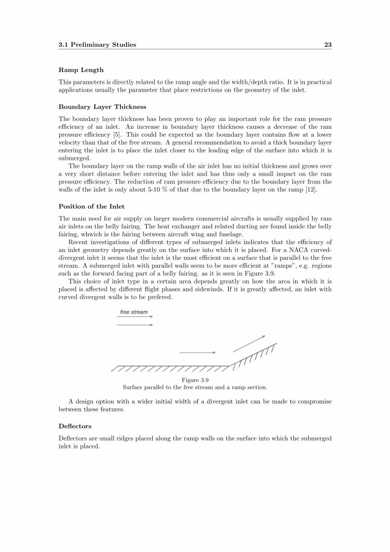
Recent investigations of different types of submerged inlets indicates that the efficiency ofan inlet geometry depends greatly on the surface into which it is placed. For a NACA curved-divergent inlet it seems that the inlet is the most efficient on a surface that is parallel to the freestream. A submerged inlet with parallel walls seem to be more efficient at ”ramps”, e.g. regionssuch as the forward facing part of a belly fairing. as it is seen in Figure 3.9.

This choice of inlet type in a certain area depends greatly on how the area in which it isplaced is affected by different flight phases and sidewinds. If it is greatly affected, an inlet withcurved divergent walls is to be prefered.

Figure 3.9Surface parallel to the free stream and a ramp section.

A design option with a wider initial width of a divergent inlet can be made to compromisebetween these features.

Deflectors

Deflectors are small ridges placed along the ramp walls on the surface into which the submergedinlet is placed.


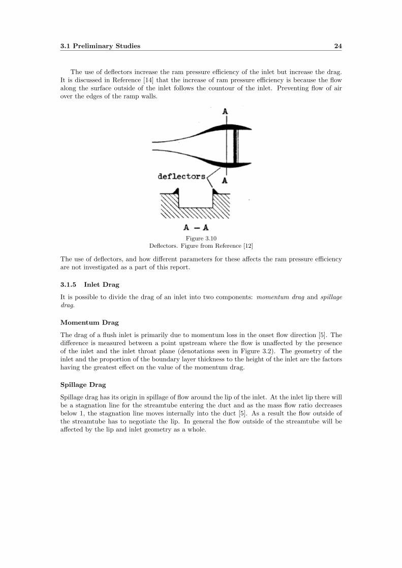
The use of deflectors increase the ram pressure efficiency of the inlet but increase the drag.It is discussed in Reference [14] that the increase of ram pressure efficiency is because the flowalong the surface outside of the inlet follows the countour of the inlet. Preventing flow of airover the edges of the ramp walls.

Figure 3.10Deflectors. Figure from Reference [12]

The use of deflectors, and how different parameters for these affects the ram pressure efficiencyare not investigated as a part of this report.

3.1.5 Inlet Drag

It is possible to divide the drag of an inlet into two components: momentum drag and spillagedrag.

Momentum Drag

The drag of a flush inlet is primarily due to momentum loss in the onset flow direction [5]. Thedifference is measured between a point upstream where the flow is unaffected by the presenceof the inlet and the inlet throat plane (denotations seen in Figure 3.2). The geometry of theinlet and the proportion of the boundary layer thickness to the height of the inlet are the factorshaving the greatest effect on the value of the momentum drag.

Spillage Drag

Spillage drag has its origin in spillage of flow around the lip of the inlet. At the inlet lip there willbe a stagnation line for the streamtube entering the duct and as the mass flow ratio decreasesbelow 1, the stagnation line moves internally into the duct [5]. As a result the flow outside ofthe streamtube has to negotiate the lip. In general the flow outside of the streamtube will beaffected by the lip and inlet geometry as a whole.


Figure 3.11The effect of mass flow ratio on the entry streamtube. Figure from Reference [5]

It is recommended that a flush inlet has a round lip, because flow separation will occur aft of thelip should the lip be too sharp [5]. However, with a rounded lip the flow still has to negotiatean adverse pressure gradient and so the boundary layer thickens and increases drag as a result.Should the gradient be large enough, a separation of the flow will occur despite the use of therounded lip [5].


3.1.6 Plenums

Two different types of plenums have previously been investigated within the ECOCENTS project.The plenum is the ”bend” section shown in the images below. The two different designs are shownin Figure 3.9 and Figure 3.10. They are refered to as the classic plenum and the base plenum.The plenum investigated in this thesis is the plenum base as it was analysed in a previous CFDstudy to perform slightly better than the classic plenum.

Figure 3.12Plenum classic. Figure from Reference [17]

Figure 3.13Plenum base. Figure from Reference [17]

3.2 Geometry Preparation 27

3.2 Geometry Preparation

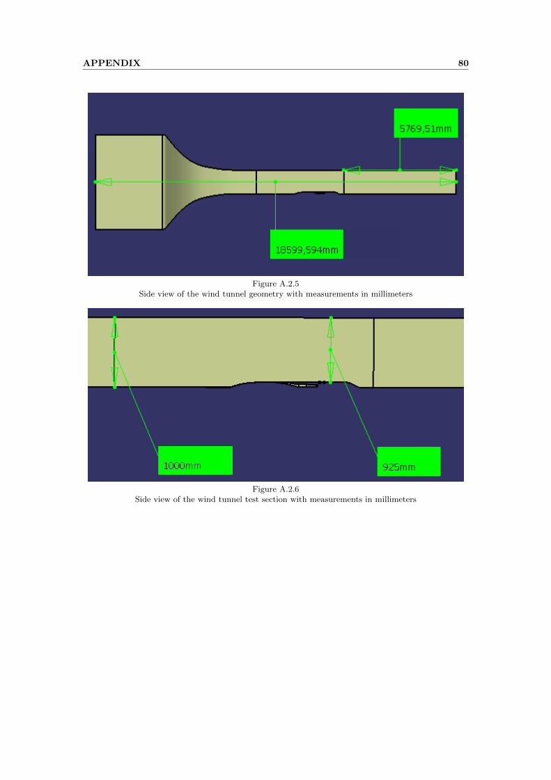
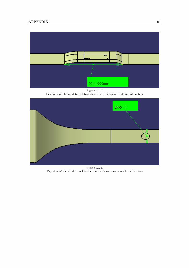
The wind tunnel geometry as well as the NACA duct geometry was provided to the author ofthis thesis by Airbus. An approximately 5.8 meter extension of the wind tunnel was made toallow the flow to stabilize aft of the test section.

Figure 3.14Original wind tunnel geometry

Figure 3.15The wind tunnel geometry with an extension aft of the test section

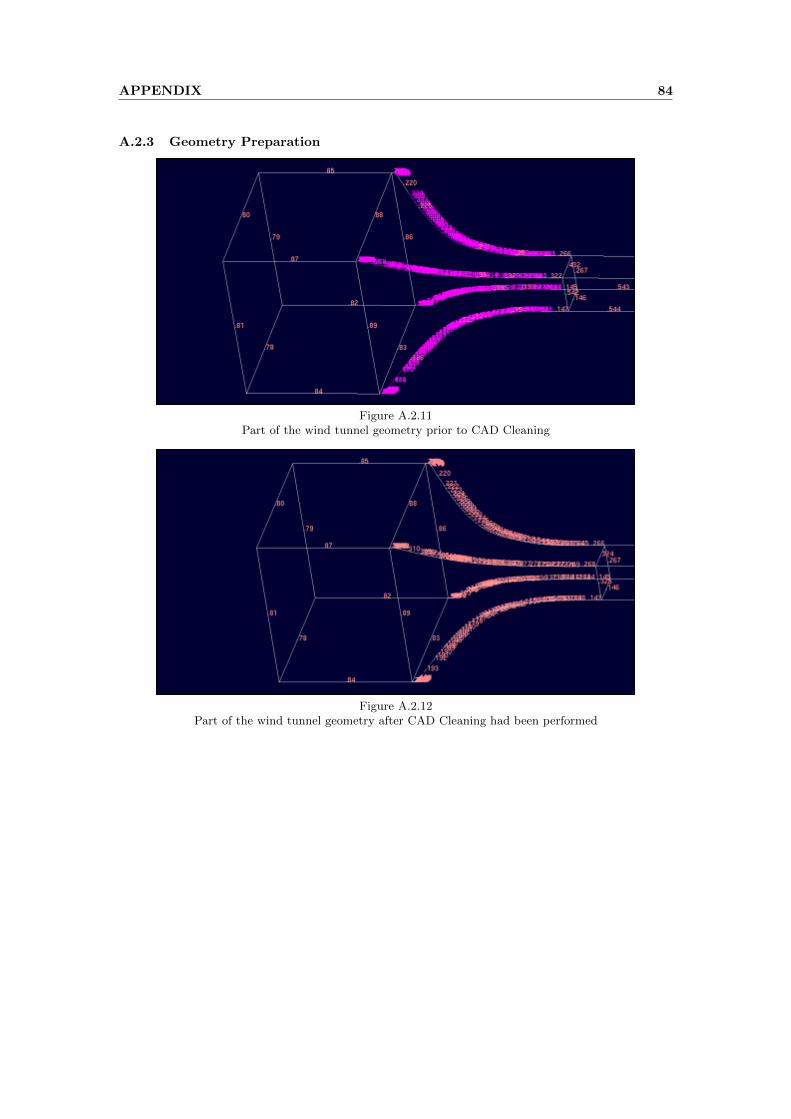
The first step of the geometry preparation process in CENTAUR was to import the IGESfile exported from CATIA. When importing an IGES file an automated query appears asking ifa CAD diagnostic should be run. The CAD diagnostic identifies problematic panels and curveswhich need to be resolved to attain a valid geometry for mesh generation. An automated CADcleaning tool can resolve some of these inconsistencies but manual labour is often necessary toresolve all issues. Figure A.2.11 and Figure A.2.12 in Appendix A2 shows a part of the windtunnel geometry before and after automated and manual CAD cleaning. A curve with a numberwritten in purple indicates that there is an issue with this curve that needs to be resolved.

The next step was to extend the wind tunnel test section. The extended test section part wasmade in CATIA and imported into CENTAUR in the correct position as the IGES file containsinformation on the coordinates of the model.

A modular mesh approach was used to minimize the time required to generate the completegrid. Modular mesh generation means that when the correct settings for the grid outside of amodular box has been found, subsequent mesh generations can be limited to the contents ofthe modular box. This saves computational time at the mesh generation stage and reduces thedifference of the final TAU results induced by the grid itself outside of the module. If we wereto generate the entire grid anew after changing the geometry, grid nodes would be generated inslightly different positions and thus have a small effect on the result.

3.2 Geometry Preparation 28

To define the boundary of the module in CENTAUR, two different approaches were available.The first was to apply the Bounding Box feature in CENTAUR and the second to create a newbox in CATIA and import the geometry into CENTAUR. The second approach was chosen andthe boundary of the module and the box itself as shown in CATIA can be seen in Figure 3.16and Figure 3.17.

Figure 3.16 Figure 3.17

The boundary of the module The module ready to be imported into CENTAUR

The ramp angle of the inlet was varied in CATIA by changing a parameter in the originalgeometry file. Models at four different ramp angles were generated:

• 4◦

• 7◦

• 10◦

• 15◦

The ramp angle of seven degrees is of main interest in this report. This is the angle recommendedby previous studies. The angle which is subject to change is the variable ramp angle shown inFigure 1.3, presented again below. The effect on the inlet and the subsequent diffuser section bya change of this angle can be seen in Figure A.2.13 - A.2.16 in Apppendix A2.


A three dimensional view of the inlet system can be seen in Figure 3.18.

3.3 Mesh Generation 29

Figure 3.18The inlet system with coordinate axis

It was suggested by Reference [18] that an extension be made to the duct after the plenumsection. The extension was recommended to be at least three times the length of the channel.This change was made directly in CENTAUR by applying the Bounding Box feature. A boundarybox consist of six panels and is defined by two sets of coordinates: minimum and maximum x,yand z-coordinates.

Figure 3.19Illustration of the extension made to the duct prior to the outlet

3.3 Mesh Generation

The prismatic elements are marched perpendicular from all surfaces with the surface elementsas basis, the best approach is therefore to generate and refine the surface mesh before generatingthe mesh in its entirety. Areas which at once could be identified as requiring refinement werethe interior of the inlet and the lip. Surface refinement in proximity to the inlet was also appliedwith geometrical sources. The lip of the inlet was refined according to the current best practicedescribed in Reference [19] with the surface element size at the outer radius of a cylinder shapedsource being 2 times the element size at the center.


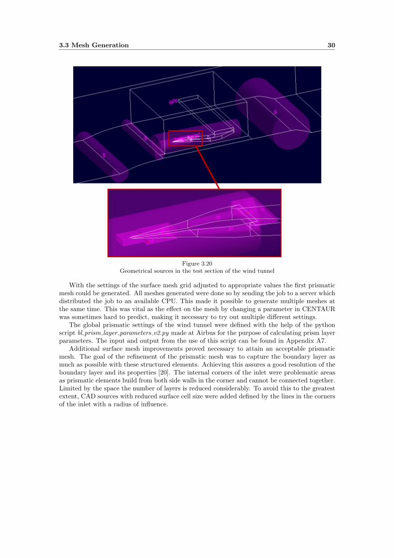
Figure 3.20Geometrical sources in the test section of the wind tunnel

With the settings of the surface mesh grid adjusted to appropriate values the first prismaticmesh could be generated. All meshes generated were done so by sending the job to a server whichdistributed the job to an available CPU. This made it possible to generate multiple meshes atthe same time. This was vital as the effect on the mesh by changing a parameter in CENTAURwas sometimes hard to predict, making it necessary to try out multiple different settings.

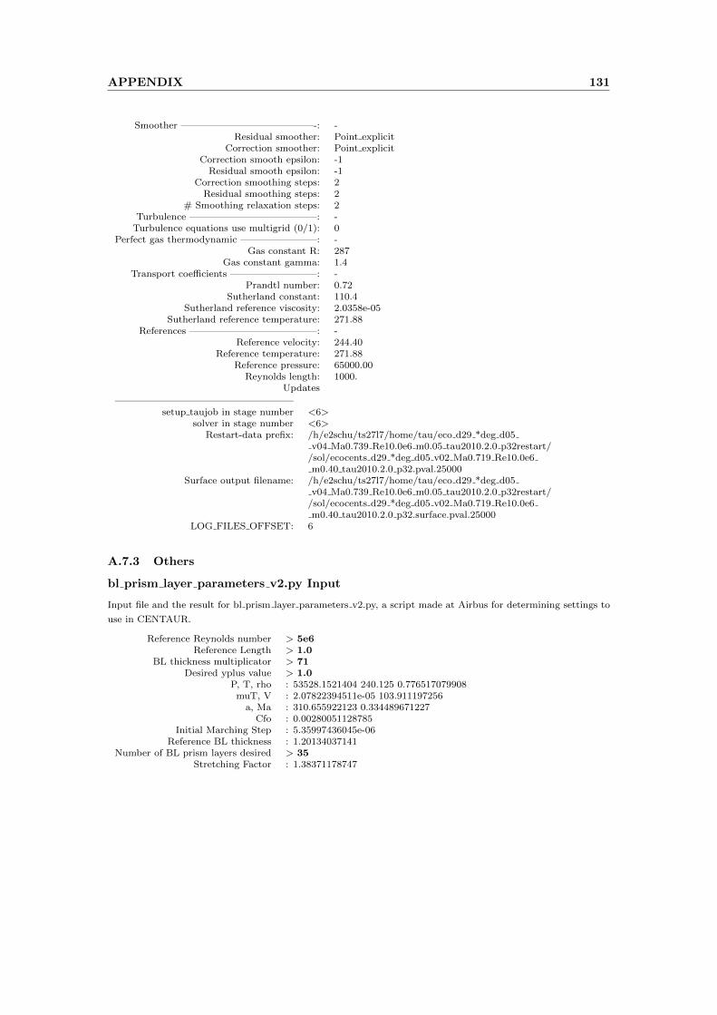
The global prismatic settings of the wind tunnel were defined with the help of the pythonscript bl prism layer parameters v2.py made at Airbus for the purpose of calculating prism layerparameters. The input and output from the use of this script can be found in Appendix A7.

Additional surface mesh improvements proved necessary to attain an acceptable prismaticmesh. The goal of the refinement of the prismatic mesh was to capture the boundary layer asmuch as possible with these structured elements. Achieving this assures a good resolution of theboundary layer and its properties [20]. The internal corners of the inlet were problematic areasas prismatic elements build from both side walls in the corner and cannot be connected together.Limited by the space the number of layers is reduced considerably. To avoid this to the greatestextent, CAD sources with reduced surface cell size were added defined by the lines in the cornersof the inlet with a radius of influence.


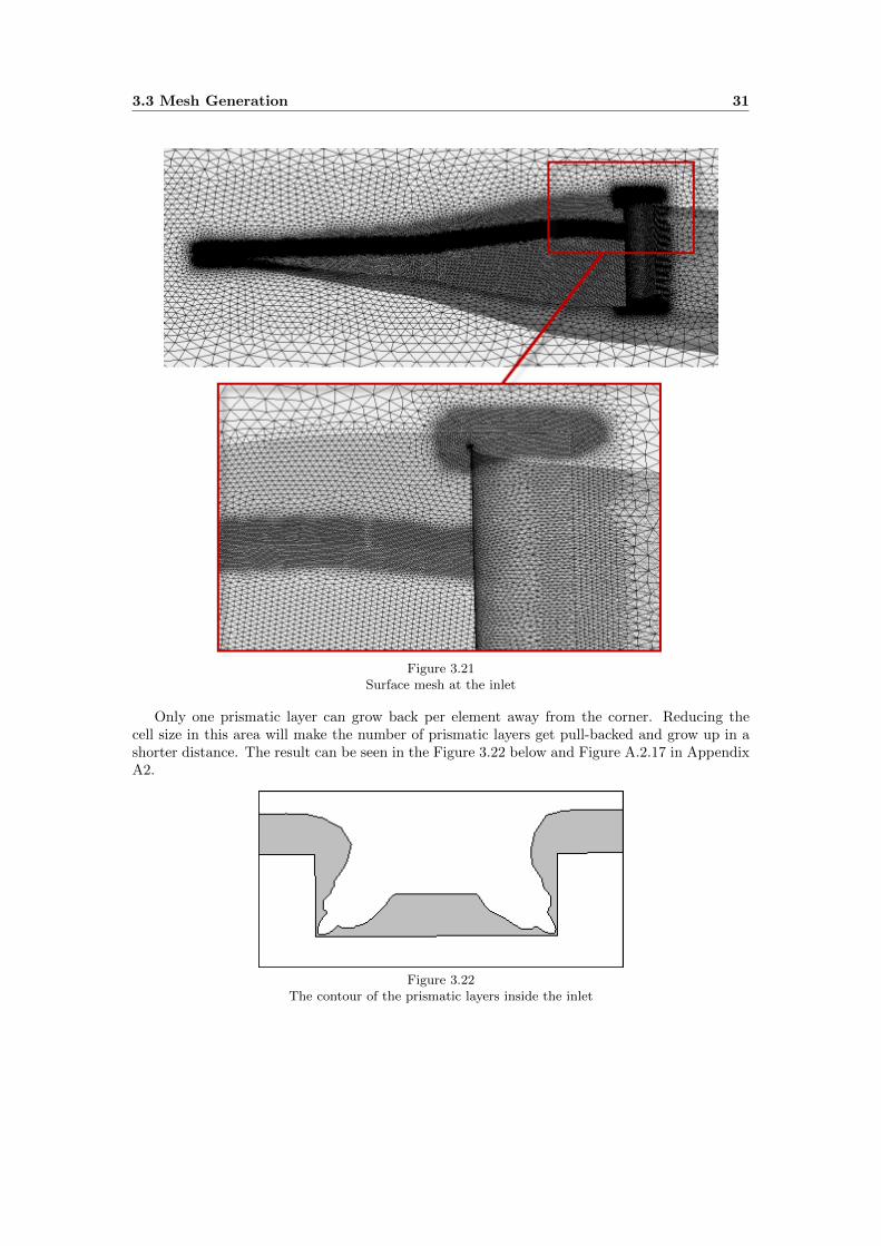
Figure 3.21Surface mesh at the inlet

Only one prismatic layer can grow back per element away from the corner. Reducing thecell size in this area will make the number of prismatic layers get pull-backed and grow up in ashorter distance. The result can be seen in the Figure 3.22 below and Figure A.2.17 in AppendixA2.

Figure 3.22The contour of the prismatic layers inside the inlet


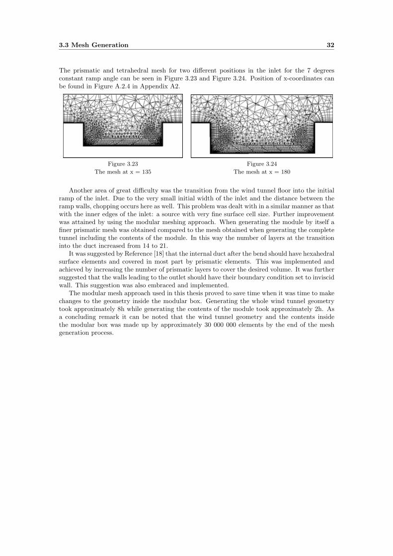
The prismatic and tetrahedral mesh for two different positions in the inlet for the 7 degreesconstant ramp angle can be seen in Figure 3.23 and Figure 3.24. Position of x-coordinates canbe found in Figure A.2.4 in Appendix A2.


The mesh at x = 135 The mesh at x = 180

Another area of great difficulty was the transition from the wind tunnel floor into the initialramp of the inlet. Due to the very small initial width of the inlet and the distance between theramp walls, chopping occurs here as well. This problem was dealt with in a similar manner as thatwith the inner edges of the inlet: a source with very fine surface cell size. Further improvementwas attained by using the modular meshing approach. When generating the module by itself afiner prismatic mesh was obtained compared to the mesh obtained when generating the completetunnel including the contents of the module. In this way the number of layers at the transitioninto the duct increased from 14 to 21.

It was suggested by Reference [18] that the internal duct after the bend should have hexahedralsurface elements and covered in most part by prismatic elements. This was implemented andachieved by increasing the number of prismatic layers to cover the desired volume. It was furthersuggested that the walls leading to the outlet should have their boundary condition set to inviscidwall. This suggestion was also embraced and implemented.

The modular mesh approach used in this thesis proved to save time when it was time to makechanges to the geometry inside the modular box. Generating the whole wind tunnel geometrytook approximately 8h while generating the contents of the module took approximately 2h. Asa concluding remark it can be noted that the wind tunnel geometry and the contents insidethe modular box was made up by approximately 30 000 000 elements by the end of the meshgeneration process.

3.4 Numerical Computation 33

3.4 Numerical Computation

The air inlet configurations investigated in this thesis were done so in a wind tunnel set-up. TheRANS solver TAU used in this thesis was originally established at DLR for external aeronau-tical flow simulations. Additional solver modules have been implemented to allow for specificsimulation problems to be solved.

The wind tunnel set-up used in TAU for this thesis was previously investigated by the softwaredevelopers in Reference [21], Reference [22] and also within a previous Airbus study (Reference[23]). The reports and presentations from DLR described two approaches within TAU to simulatewind tunnels:

• Wind Tunnel Boundary Condition [21]

• Engine Boundary Condition [21]

Both numerical approaches require similar inputs for the boundary conditions, only some ofthe physical variable names are different. The results of both approaches are expected to beequal.

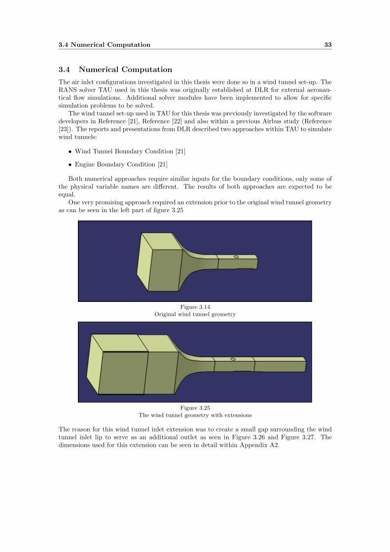
One very promising approach required an extension prior to the original wind tunnel geometryas can be seen in the left part of figure 3.25

Figure 3.14Original wind tunnel geometry

Figure 3.25The wind tunnel geometry with extensions

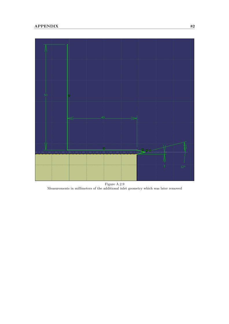
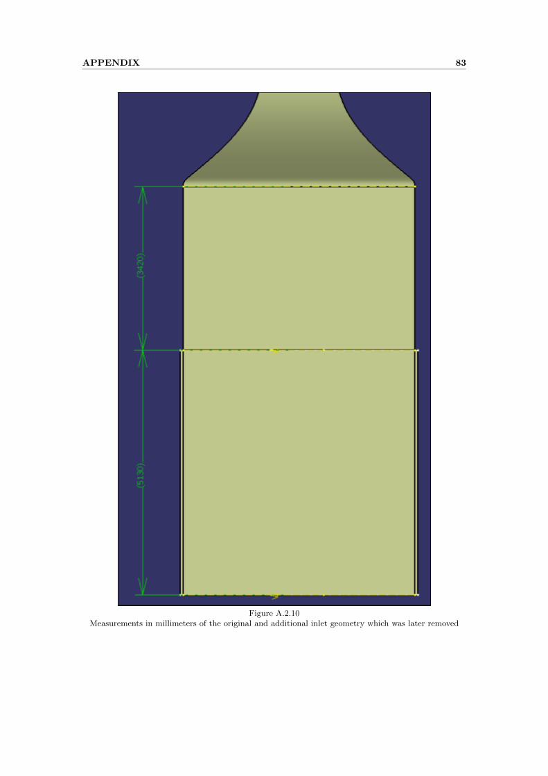
The reason for this wind tunnel inlet extension was to create a small gap surrounding the windtunnel inlet lip to serve as an additional outlet as seen in Figure 3.26 and Figure 3.27. Thedimensions used for this extension can be seen in detail within Appendix A2.



Computational grid at the additional outlet Velocity profiles at the additional outlet

Figure from Reference [21] Figure from Reference [21]

This set-up has the big advantage to define wind tunnel inlet condition for the RANS compu-tations in a single point within the inlet plane, similarly as it would be measured in wind tunneltests. The wind tunnel inlet extension was considered to be an inviscid wall, hence the meshcontained tetrahedras similarly to how it is seen in Figure 3.26.

Reference [21] describes that this additional outlet would act in conjugation with the simu-lation inlet plane such that the requested physical condition will be iteratively adjusted for theintroduced reference point. Figure 3.28 Shows that adjustment approach.

Figure 3.28Schematic set-up of the numerical wind tunnel simulation.

Wind tunnel extension (inviscid wall) not to scale

This promising approach was persued to great length, and with technical reports by DLR[21] it was believed that it would work for the geometrical set-up in this thesis. However, withinthe work of this thesis it was impossible to get the numerical computations to run stable overa certain iteration number. The reason for this unstable numerical behaviour is seen in thedifficulty for the solver to get adjusted two reference points. This problem was impossible tosolve by varying the intervall steps between iterations for when flow parameters were adjusted.

It turned out that in order to achieve the goal of this thesis a more basic approach had tobe used. The additional geometry prior to the original wind tunnel inlet had to be removed andthe boundary condition ”wind tunnel inlet” was applied at the wind tunnel inlet plane.

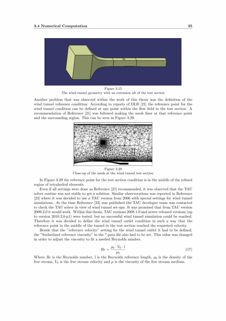
The final numerical wind tunnel set-up that was used within this thesis is seen in Figure 3.15below.


Figure 3.15The wind tunnel geometry with an extension aft of the test section

Another problem that was observed within the work of this thesis was the definition of thewind tunnel reference condition: According to reports of DLR [21] the reference point for thewind tunnel condition can be defined at any point within the flow field in the test section. Arecommendation of Reference [21] was followed making the mesh finer at that reference pointand the surrounding region. This can be seen in Figure 3.29.

Figure 3.29Close-up of the mesh at the wind tunnel test section

In Figure 3.29 the reference point for the test section condition is in the middle of the refinedregion of tetrahedral elements.

Even if all settings were done as Reference [21] recommended, it was observed that the TAUsolver routine was not stable to get a solution. Similar observerations was reported in Reference[23] where it was decided to use a TAU version from 2006 with special settings for wind tunnelsimulations. At the time Reference [23] was published the TAU developer team was contactedto check the TAU solver in view of wind tunnel set-ups. It was promised that from TAU version2009.2.0 it would work. Within this thesis, TAU versions 2008.1.0 and newer released versions (upto version 2010.2.0-p1) were tested, but no successful wind tunnel simulation could be reached.Therefore it was decided to define the wind tunnel outlet condition in such a way that thereference point in the middle of the tunnel in the test section reached the requested velocity.

Beside that the ”reference velocity” setting for the wind tunnel outlet it had to be defined,the ”Sutherland reference viscosity” in the *.para file also had to be set. This value was changedin order to adjust the viscosity to fit a needed Reynolds number.

Re =ρ0 · V0 · l

µ0(17)

Where Re is the Reynolds number, l is the Reynolds reference length, ρ0 is the density of thefree stream, V0 is the free stream velocity and µ is the viscosity of the free stream medium.


The value of l was chosen to be 1.0m, as for wind tunnel measurements the test sectiondiameter or a relation of the square cross section area is used instead of any reference length ofthe tested model. TWG has a test section area of 1.0m x 1.0m, without consideration of theused ramp.

3.5 Post Processing 37

3.5 Post Processing

When the values of the variables defined in the *.para file had been found, the different geometriescould be submitted to a specified number of processors.

Shown below is the pressure distribution and Mach number in the tunnel for a configurationwith Mach number 0.8 above the inlet in the test section.

Figure 3.30Side view of the wind tunnel showing the pressure distribution in Tecplot 360

Figure 3.31Side view of the wind tunnel showing the Mach number in Tecplot 360

The boundary layer thickness was investigated with usage of Tau BL to verify that the prismaticlayers cover the boundary layer. This investigation showed that the boundary layer was thickerthan the prismatic layers at some points in the mesh, resulting in some additional adjustments.This can be seen when comparing the last and second last pictures in Figure A.3.11 in AppendixA3.

The residual of the calculations in TAU is a measure of the accuracy of the solution. Thenumerical residual represents the numerical rest terms after each iteration step. A smaller valueindicates higher accuracy. The inlet presence has a great impact on the accuracy of the numericalsolution. This influence is mainly due to two circumstances: first, the additional boundarycondition ”outlet” for the NACA inlet configuration makes it more difficult for the solver to geta converged solution. Additionally, the NACA inlet itself has an immence physical influence onthe flow. Beside wakes outside and inside the NACA inlet, it is also difficult for the TAU solverto simulate the low flow velocities (Mach < 0.15). In Figure 3.32 and 3.33 are seen residual plotsfor a clean wind tunnel setup and a wind tunnel setup with an inlet, respectively.

3.5 Post Processing 38

Figure 3.32Residual plot for the clean wind tunnel setup. From 0 to 25 000 iterations.

Figure 3.33Residual plot for the wind tunnel with an inlet. From 0 to 25 000 iterations.

It should be remarked that the numerical calculations are driven much further in view ofnumber of iterations than can be seen in Figure 3.33. The converged solution of an inlet con-figuration was obtained at approximately 200 000 iterations. The residual and physical values(e.g. drag) was observed during the computations in order to secure a converged solution andtherefore valuable results.

The drag of the assembly parts that were defined in CENTAUR was stated in the end of theconverged TAU solution. This aerodynamic drag is splitted within TAU into two parts: pressuredrag and viscous drag.

3.6 Empirical Method Analysis 39

3.6 Empirical Method Analysis

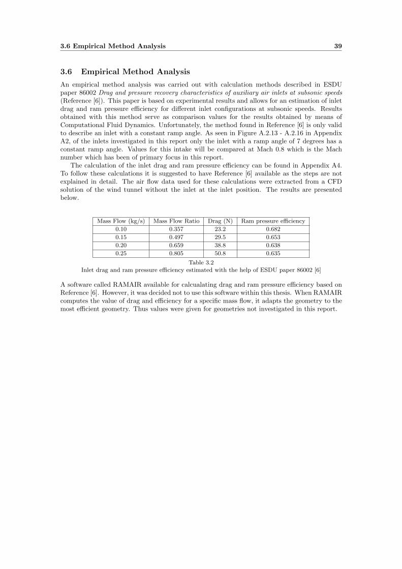
An empirical method analysis was carried out with calculation methods described in ESDUpaper 86002 Drag and pressure recovery characteristics of auxiliary air inlets at subsonic speeds(Reference [6]). This paper is based on experimental results and allows for an estimation of inletdrag and ram pressure efficiency for different inlet configurations at subsonic speeds. Resultsobtained with this method serve as comparison values for the results obtained by means ofComputational Fluid Dynamics. Unfortunately, the method found in Reference [6] is only validto describe an inlet with a constant ramp angle. As seen in Figure A.2.13 - A.2.16 in AppendixA2, of the inlets investigated in this report only the inlet with a ramp angle of 7 degrees has aconstant ramp angle. Values for this intake will be compared at Mach 0.8 which is the Machnumber which has been of primary focus in this report.

The calculation of the inlet drag and ram pressure efficiency can be found in Appendix A4.To follow these calculations it is suggested to have Reference [6] available as the steps are notexplained in detail. The air flow data used for these calculations were extracted from a CFDsolution of the wind tunnel without the inlet at the inlet position. The results are presentedbelow.

Mass Flow (kg/s) Mass Flow Ratio Drag (N) Ram pressure efficiency

0.10 0.357 23.2 0.682

0.15 0.497 29.5 0.653

0.20 0.659 38.8 0.638

0.25 0.805 50.8 0.635

Table 3.2Inlet drag and ram pressure efficiency estimated with the help of ESDU paper 86002 [6]

A software called RAMAIR available for calcualating drag and ram pressure efficiency based onReference [6]. However, it was decided not to use this software within this thesis. When RAMAIRcomputes the value of drag and efficiency for a specific mass flow, it adapts the geometry to themost efficient geometry. Thus values were given for geometries not investigated in this report.

3.6 Empirical Method Analysis 40

4 Results and Discussion 41

4 Results and Discussion

4.1 Pressure and Mach number Analysis

In this section the physical flow features of the NACA inlet are analysed. For the most figures,the inlet with a 7 degrees ramp angle is used to illustrate the flow effects.

Figure 4.1Side view in the symmetry plane of the inlet showing the Mach number

Mach 0.8. 7 degrees ramp angle. Mass flow: 0.20 kg/s

It can be seen in Figure 4.1 that the Mach number is decreased in the area outside of the inlet.The region of low velocity flow closest to the wind tunnel surface is thinner aft of the inlet lip asmost of the boundary layer has been sucked in by the inlet.

At the lip of the inlet a local region can be observed where the flow velocity is decelerated.Even if it is not clearly seen in Figure 4.1, there is also a stagnation point at the lip. Along thebottom side of the lip there is an acceleration of the flow and in a small area the velocity is abovethat of the free stream.

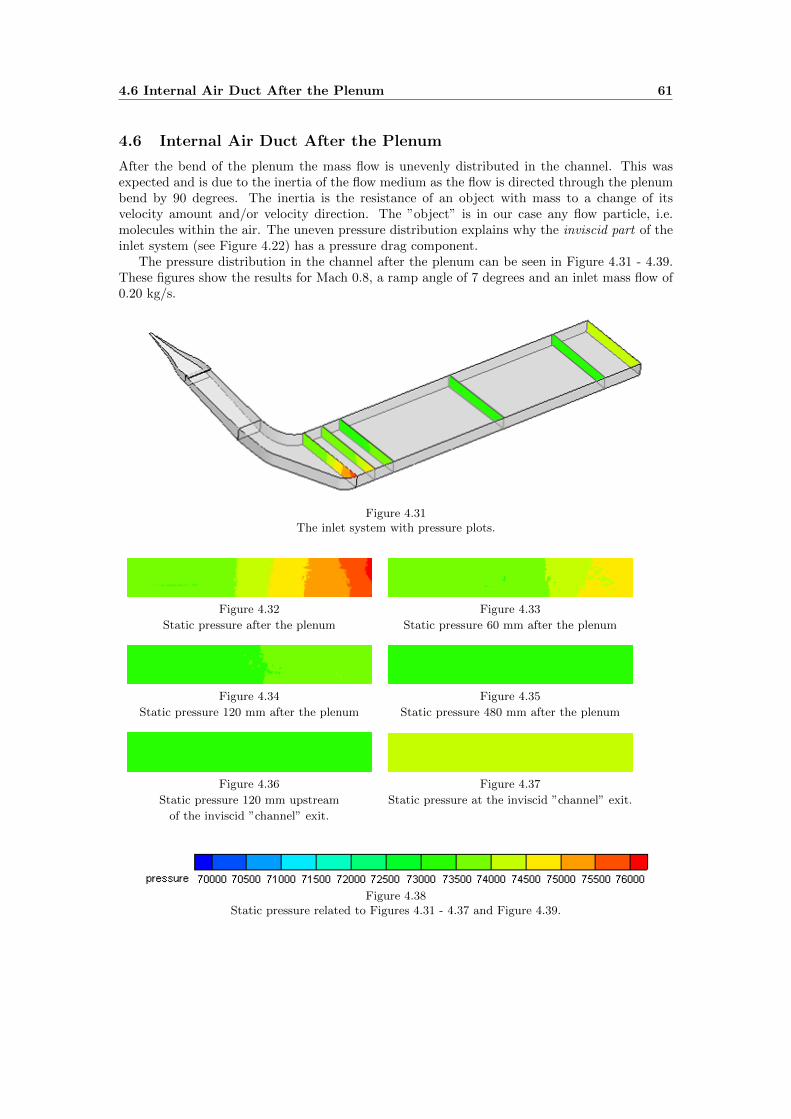
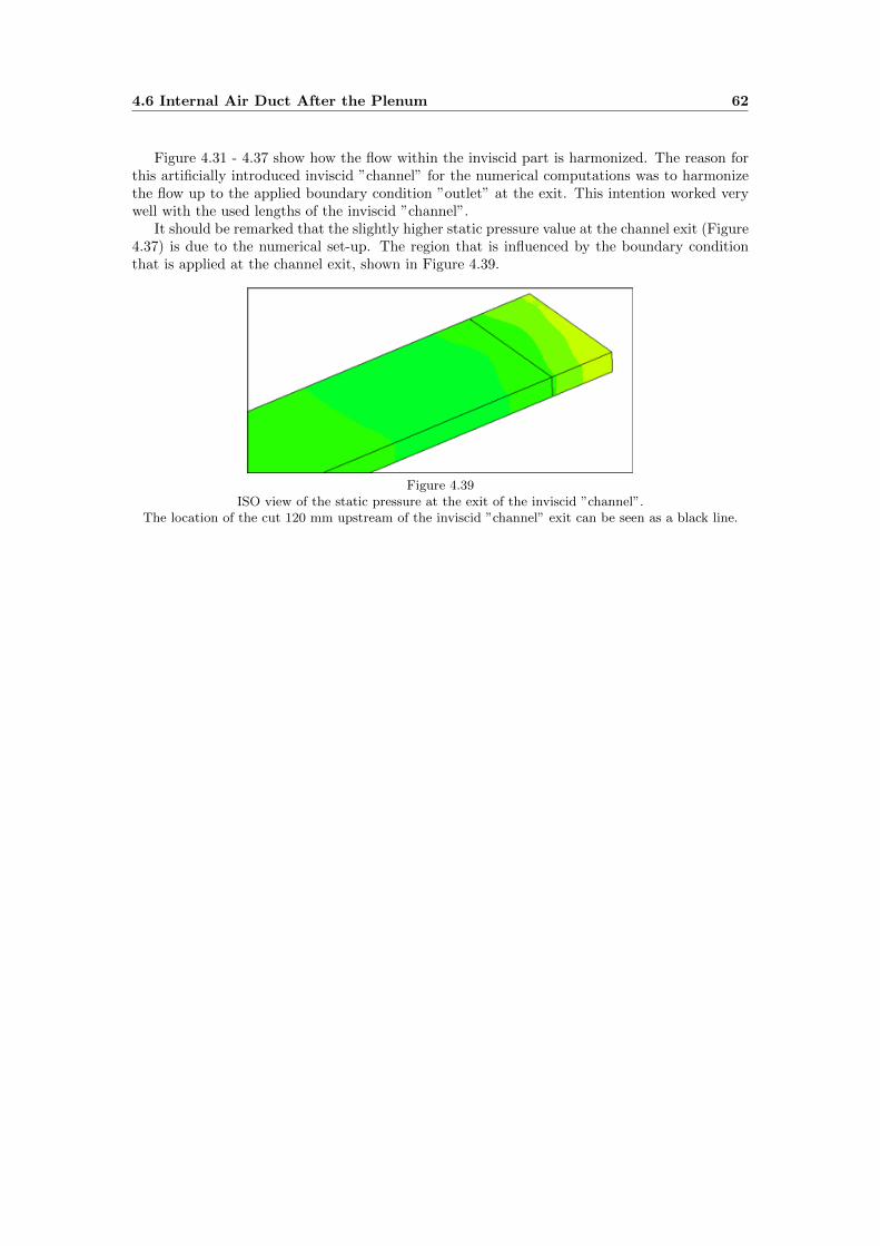
As the air flows further down into the diffuser the velocity of the flow becomes more uniform.As the air is lead through the inlet and down into the diffuser it will have a velocity componentdownwards. When the flow reaches the end of the diffuser and into the plenum, which is parallelto the wind tunnel floor, the flow will initially be located mostly in the lower region of thechannel. This can be seen illustrated in Figure 4.6 and Figure 4.7 in the next section.

For the same configuration at a higher mass flow the air flow reaches sonic speed (Ma = 1.0)at the beginning of the diffuser as can be seen in Figure 4.2. This reduces the total pressure ofthe flow and indicates that the throat of the inlet is now choking, which means that no additionalair will pass the throat. At which mass flow this occurs depend greatly on the flow condition inthe free stream and the pressure acting at the end of the inlet system.



4.1 Pressure and Mach number Analysis 42

Figure 4.3Side view in the symmetry plane of the inlet showing the static pressure


Figure 4.3 illustrates a great increase of static pressure at the stagnation point of the inlet lip.This figure also shows that the static pressure rises along the flow direction within the diffuser.This effect is due to the reduction of the flow velocity within the diffuser while the total pressureis nearly constant, as it is seen in Figure 4.4.

Figure 4.4Side view in the symmetry plane of the inlet showing the total pressure


Figure 4.4 shows an expected behaviour of the total pressure: In general, the total pressure islower with approximation to any surface. This effect is mainly caused by the friction of thesurface. In Figure 4.4 is also seen the influence of the NACA inlet on the total pressure. Itshould be remarked that the total pressure and static pressure in combination give an overallpicture of the situation, since Ptot = Pstat + Pdyn.

When the total pressure within the inlet and channel is nearly constant while the staticpressure is increasing, it means that the dynamic pressure is decreasing. This was also expectedsince the flow velocity is decreasing as the flow drives through the inlet and diffuser.

4.2 Boundary Layer Analysis 43

4.2 Boundary Layer Analysis

As a part of this thesis the boundary layer before, inside and aft of the inlet is analysed. The airflow into the inlet can be illustrated with the help of streamtraces placed in the free stream priorto the inlet. A streamtrace is the path of a massless particle placed in the free stream. Thesestreamtraces show how the air closest to the wind tunnel surface flows into the inlet.

Figure 4.5Top view of the inlet with the positions of the cuts shown in Figure 4.6 - 4.8.

Figure 4.6Side view in the symmetry plane of the inlet with streamlines. Cut 1

Figure 4.7Side view of the inlet 19 mm to one side of the symmetry plane. Cut 2. Total width of inlet is 75 mm

Figure 4.8Side view 38 mm to one side of the inlet symmetry plane. Cut 3. Total width of inlet is 75 mm

In Figure 4.6 the air flow at the surface and a relatively large region away from the surfaceis sucked into the inlet. In the next figure, Figure 4.7, a smaller region of air enters the inletcompared to at the symmetry plane of the inlet shown in Figure 4.6. The influence region of theinlet is smaller compared to the symmetry plane (cut 1). In Figure 4.8 the flow is not seen to


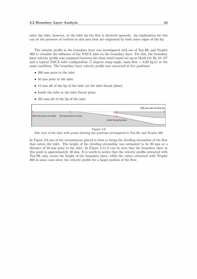
enter the inlet, however, at the inlet lip the flow is diverted upwards. An explanation for thiscan be the presence of vortices in this area that are originated by both outer edges of the lip.

The velocity profile in the boundary layer was investigated with use of Tau BL and Tecplot360 to visualise the influence of the NACA inlet on the boundary layer. For this, the boundarylayer velocity profile was compared between the clean wind tunnel set-up at Mach 0.8, Re 10 ·106

and a typical NACA inlet configuration (7 degrees ramp angle, mass flow = 0.20 kg/s) at thesame condition. The boundary layer velocity profile was extracted at five positions:

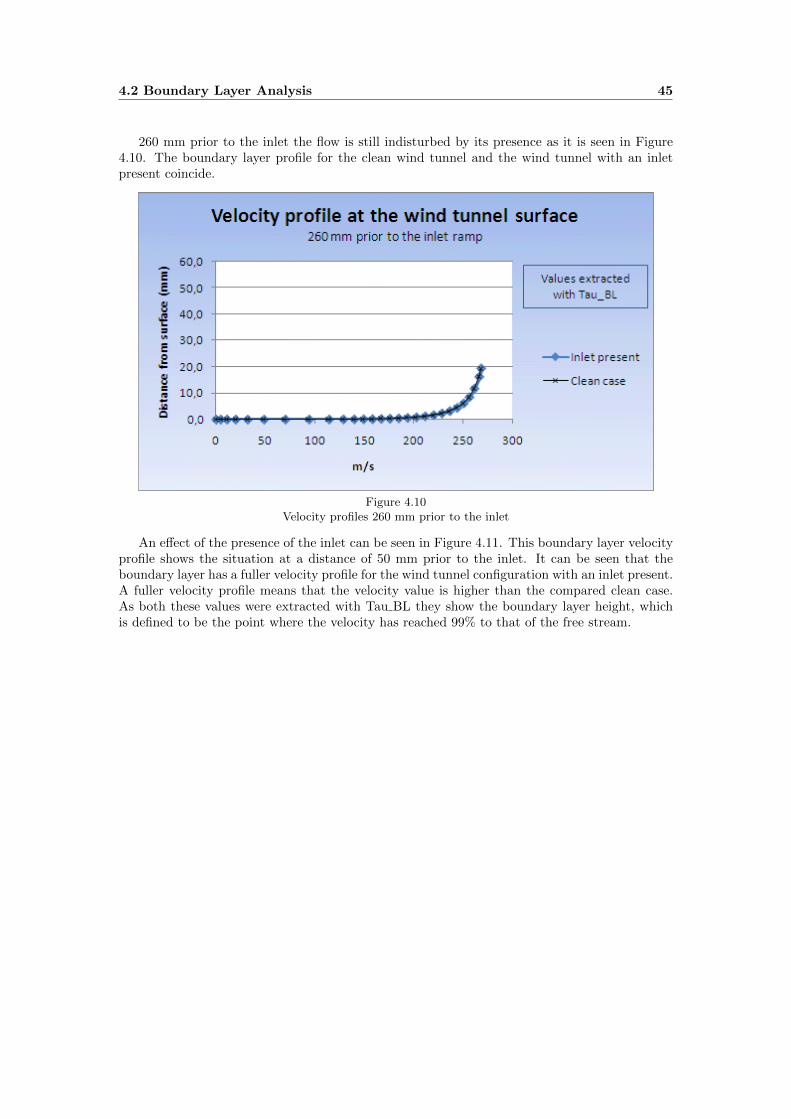
• 260 mm prior to the inlet

• 50 mm prior to the inlet

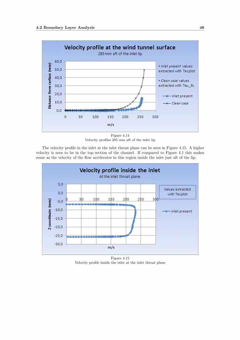
• 15 mm aft of the lip of the inlet (at the inlet throat plane)

• Inside the inlet at the inlet throat plane

• 285 mm aft of the lip of the inlet

Figure 4.9Side view of the inlet with points showing the positions investigated in Tau BL and Tecplot 360

In Figure 4.6 one of the streamtraces placed is close to being the dividing streamline of the flowthat enters the inlet. The height of the dividing streamline was estimated to be 20 mm at adistance of 50 mm prior to the inlet. In Figure 4.11 it can be seen that the boundary layer atthis point is approximately 40 mm. It is worth to notice that the velocity profile extracted withTau BL only covers the height of the boundary layer, while the values extracted with Tecplot360 in some cases show the velocity profile for a larger portion of the flow.


260 mm prior to the inlet the flow is still indisturbed by its presence as it is seen in Figure4.10. The boundary layer profile for the clean wind tunnel and the wind tunnel with an inletpresent coincide.

Figure 4.10Velocity profiles 260 mm prior to the inlet

An effect of the presence of the inlet can be seen in Figure 4.11. This boundary layer velocityprofile shows the situation at a distance of 50 mm prior to the inlet. It can be seen that theboundary layer has a fuller velocity profile for the wind tunnel configuration with an inlet present.A fuller velocity profile means that the velocity value is higher than the compared clean case.As both these values were extracted with Tau BL they show the boundary layer height, whichis defined to be the point where the velocity has reached 99% to that of the free stream.


Figure 4.11Velocity profiles 50 mm prior to the inlet

15 mm aft of the inlet lip it can be seen that the boundary layer has grown for the clean caseas to be exptected. For the case with the inlet, a large portion of the low-velocity air flow hasentered the inlet and a boundary layer is now growing up with a starting pont at the inlet lip.

Figure 4.12Velocity profiles 15 mm aft of the inlet lip

In Figure 4.13 the velocity profile for the flow close to the wind tunnel surface can again be seenfor the point 15 mm aft of the inlet. The distance to the surface (y-axis) is zoomed. Only the


curve representing the velocity profile with the inlet present is shown. In this figure it can beseen that the boundary layer is very thin at this point, approximately 1 mm.

Figure 4.13Detailed velocity profile 15 mm aft of the inlet lip with the inlet present

A point 285 mm aft of the inlet was investigated to show that the shape and height of theboundary layer for the case with the inlet now is clearly seen in relatation to the clean case.The boundary layer of the case with a NACA inlet has further developed, but a difference to theclean case is still visible. It should be remarked that the free stream velocity is slightly higherfor the clean case. This is seen in the last shown point of each case (contrary to the point 50mm prior to the inlet).


Figure 4.14Velocity profiles 285 mm aft of the inlet lip

The velocity profile in the inlet at the inlet throat plane can be seen in Figure 4.15. A highervelocity is seen to be in the top section of the channel. If compared to Figure 4.1 this makessense as the velocity of the flow accelerates in this region inside the inlet just aft of the lip.

Figure 4.15Velocity profile inside the inlet at the inlet throat plane


4.2.1 Ramp wall edges

In order to investigate the effect of sharp ramp wall edges on the boundary layer air that flowsover the edges into the inlet (described in section 3.1.2), streamtraces were placed on the surfaceprior to the inlet. This is shown in Figure 4.16 below. These streamtraces showed that withsharp edges, flow will still be going into the duct from the sides. This observation was expected,since we have a lower pressure inside the duct than outside, driving the flow.

In Figure 4.16 is also visible the influence of the wakes that enters the inlet. The placedstreamlines are swirled and enter the intake section.

Figure 4.16Streamtraces placed at the NACA submerged inlet from a Tau BL solution as seen in Tecplot 360

The loss of pressure described in Reference [15] was discussed with Reference [24] and the agreedinterpretation was that the loss of pressure resulting from rounded edges was due to the vorticesnot forming along the rounded ramp edges.


4.3 Ram Pressure Efficiency

The ram pressure efficiency is used in this report to judge the effictiveness of the investigated airinlet. The values obtained for this parameter can be compared to earlier studies and additionally,this comparison is also a check of the reliability of the results.

The turbulence model used in this thesis was the SAE (Spalart-Allmaras with Edwardsmodification) model. The subject of this thesis was an investigation of the inlet efficiency, not astudy of different turbulence models. A previous study, Reference [1], made a similar investigationof NACA inlets at low speed using the TAU RANS solver. Reference [1] investigated two differentturbulence models and compared the results to NACA experimental results. The comparisoncan be seen in Figure 4.17.

Figure 4.17Ram pressure efficiency comparison at Mach 0.2 for different turbulence modelsNACA experimental results graph has been adjusted. Figure from Reference [1]

It can be seen that for velocity ratios greater than 0.4 there is very little difference in the re-sults obtained with the applied turbulence models. For lower velocity ratios the SST turbulencemodel comes closer to experimental results. All results evaluated in this thesis, except for onone occation (7 degrees ramp angle, 0.10 kg/s mass flow, Mach 0.8) have a velocity ratio greaterthan 0.4. Therefore the SAE turbulence model was chosen. Another reason for choosing theSAE model was because of the higher experience reliability with this model. It is also known tobe robust and fast convergent.

The RANS solver results of this thesis were compared to own estimations, based on ESDUpaper 86002 (Reference [6]). This method is based on NACA experimental results and takesamong others, following parameters into account: the geometry of the inlet, the free streamvelocity and the boundary layer thickness. Even though ESDU method is proven to predict themain flow physics, previous studies [25] have shown an off-set in results between ESDU and CFDobtained results. With this in mind it can be expected that the results in this thesis will differin some degree to ESDU results.


An additional comparison is made to values obtained with a different flow solver (Star-CCM+v.4.06) for the same NACA inlet geometry placed in the same wind tunnel (TWG) as investigatedwithin this thesis.

The results have been compared for one geometry, the seven degrees constant ramp angle.The comparison has been limited to this geometry because the method described by ESDU isonly valid for a constant ramp angle. That angle is the selection 7 degrees ramp case.

Figure 4.18Ram pressure efficiency comparison for different estimation methods

It can be seen that ESDU predicts a higher ram pressure efficiency than TAU. The tendency ofthe curve does however seem to be very similar.

Star-CCM+ predicts an even lower efficiency for the same conditions. It is expected that thislower ram pressure efficiency in some extent can be explained by the presence of the (unheated)heat exchanger after the plenum. The heat exchanger represents for the internal flow anotherchange of the flow direction and hence another reduction of the flow velocity. This effect isexpected to influence the upstream flow and therefore also the Ram pressure efficiency. It isdifficult to judge the influence of that heat exchanger. This influence will be cleared by asuccessive TAU CFD investigation that will contain heat exchanger and RAO (ram air outlet).Additionally, the TWG wind tunnel campaign in autumn 2011 will contribute to this subject.

Figure 4.19 shows a comparison for Star-CCM+ and TAU for all ramp angles investigated.It can be seen that compared to the results obtained with Star-CCM+ the results obtained withTAU does not show a great reduction of ram pressure efficiency for different mass flows. Thiscould also be an influence of the heat exchanger and RAO, that might be more sensitive to verylow internal flows.


Figure 4.19Ram pressure efficiency comparison for different mass flows

Figure 4.20 shows a comparison of TAU results on RAM pressure efficiency between the fourdifferent ramp angles investigated in this report at Mach 0.8. In the graph a local maximum ofthe ram pressure efficiency can be seen for the 10 and 15 degrees ramp angle in the middle of thesimulated mass flow values. Contrary, for inlet ramp angles 4 and 7 degrees the most efficientregions seem to be at lower mass flows.

Figure 4.20Ram pressure efficiency for different inlet ramp angles in relation to the mass flow

4.4 Ram Recovery Ratio 53

4.4 Ram Recovery Ratio

The investigation of pressure loss was extended up to the diffuser. This ratio is named ramrecovery ratio. It can be seen in Figure 4.21 that the total pressure is decreased more overthe diffuser with increasing mass flow and reduced ramp angle. The reduction of ramp angleis directly connected to the angle between the upper and lower diffuser walls. A small inletramp angle is followed by a larger diffuser angle than at higher inlet ramp angles. The lowerram recovery ratio after the diffuser for smaller ramp angles can be explained by the small inletthroat area followed by a large diffuser angle.

Table A.5.2 in Appendix A5 shows the diffuser angles for the different inlet ramp angles.

Figure 4.21Ram recovery ratio for different inlet ramp angles in relation to the mass flow

4.5 Drag investigation 54

4.5 Drag investigation

The drag output from the flow solver TAU is given separately as pressure drag and viscousdrag for different assembly parts. The assembly parts were defined according to how they weregrouped together in CENTAUR. The naming and definition of the different sections in this thesiscan be seen in Figure 4.22 and Figure 4.23.

Figure 4.22Naming of the different inlet system assembly parts in this thesis

Figure 4.23Naming of the wind tunnel test section parts in this thesis

The drag output of from TAU is given as a drag coefficient CD, based on the reference area inthe TAU input file. This value can be reconverted into drag in Newton with the use of Equation(1) in this thesis. The values needed to use this equation are additionally the reference area,reference velocity and reference density that were defined in the TAU input.


When calculating the drag caused by only the inlet, the drag of the inlet assembly componentwas included as well as the resulting increase of drag on the module floor and test section floor.

When calculating the drag caused by the inlet system, the included parts are the inlet,diffuser, plenum, inviscid part and the resulting increase of drag on the module floor and testsection floor.

When comparing values to ESDU it must be remembered that ESDU estimates the dragcaused by the presence of the inlet only. None of the other inlet system parts and surroundingsurfaces are considered within the ESDU method. Figure 4.24 shows the comparison of theinvestigated assembly parts for TAU vs. ESDU.

Figure 4.24Drag comparison for the 7 degrees ramp angle configuration

It is seen a big difference in the results of both methods. The discrepancy between the TAURANS solver and the ESDU method can be explained by that ESDU consider the inlet but alsoinclude drag terms that are derived by the inlet presence.The drag terms are ram drag, spillagedrag and skin friction drag. Within ESDU any influence downstream of the inlet itself is notincluded. Therefore the bend of the plenum is ignored within ESDU.

In contrast to ESDU, with TAU it is impossible to split drag into drag components. WithinTAU it is only possible to consider the drag contribution of assembly parts, as seen in Figure 4.22.These parts does contain all drag components but it is impossible to extract their contribution tothe drag in detail. Therefore in Figure 4.24, the graph of ESDU should be compared with ”TAUinlet system”. It should be remarked that in the TAU results, the plenum bend is included. Thedifference between TAU and ESDU of around 9 Newton is seen to originate in some parts bythe presence of the plenum bend. Moreover, similar underpredictions of ESDU were reportedby Reference [24] and Reference [26] that were involved in the design process of several aircraftsand in different research projects. A similar underprediction of ESDU was observed recently ina different inlet design, where TAU RANS results coincide with a completely different RANSsolver ELSA, using structured meshes.


Figure 4.25Drag comparison for the different ramp angles at Mach 0.8

Figure 4.25 shows the drag comparison of the inlet assembly parts for different ramp angles. Itcan be seen in that figure that for the region of lower mass flows (0.10 - 0.15 kg/s) the 7 degreesramp angle has the lowest drag. At 0.25 kg/s the 7 degrees ramp angle again seem to be theinlet which has the lowest value of drag, however, at this mass flow the flow inside the diffuser isMa = 1.0 as can be seen in Figure 4.26. It is interpreted from the graph in Figure 4.25 and theplot in Figure 4.26 that flow ”choking” in the throat has just started at that mass flow value of0.25 kg/s. A similar region of sonic flow is seen for the 4 degrees ramp angle at 0.20 kg/s.



For an increase of the mass flow to the region of 0.20 - 0.30 kg/s the 10 degrees ramp angle hasthe lowest drag and therefore seems to be the best choice.


As it was discussed earlier, a more realistic consideration is seen in the drag analysis of thecomplete inlet system. Figure 4.27 shows this.

Figure 4.27Drag comparison for the different angles for the complete inlet system at Mach 0.8

A difference that can be noted when comparing Figure 4.26 and Figure 4.27 is that the 7 degreesramp angle seems more efficient at a mass flow of 0.20 kg/s when comparing the whole inletsystem. This result is expected to be more realistic since the drag contributions of all the inletsystem assembly parts are taking into account.

In Figure 4.28 is shown the comparison of the total drag for the complete inlet system fordifferent Mach numbers. It is seen that drag increases with rising Mach numbers. This effectwas also expected since the higher velocity contributes mainly additional pressure drag. Thedrag tendency has a linear behavior with increasing mass flow. This is valid for all investigatedMach numbers.


Figure 4.28Drag comparison for 7 degrees ramp angle for the complete inlet system at different Mach numbers

Within this thesis additionally also a variation of the Reynolds number was investigated. Thevalue of the Reynolds number used within this thesis was 10 ·106. Additionally 5 ·106 and 15 ·106

were investigated for a constant ramp angle of 7 degrees at Mach 0.8. The Reynolds number wasvaried by adjusting the viscosity of the flow medium.

In Figure 4.29 the effect of Reynolds number variation on the complete air inlet system isshown.


Figure 4.29Drag comparison for 7 degrees ramp angle for complete inlet system at different Reynolds numbers

As expected, the Reynolds number influences the flow characteristics. With rising Reynoldsnumber the dynamic viscosity decreases. At high Reynolds numbers the drag dependency on thevelocity of the air is increased. When the Reynolds number is increased, the drag is increaseseven though the velocity of the medium is approximately the same. This increase of drag is notlinear, a further increase of the Reynolds number above 15 · 106 would only increase the totaldrag slightly.

For one case the contribution to the total amount of drag of the inlet system has been extracedfor each inlet system assembly part. The case represented in Figure 4.30 is the 7 degrees rampangle at Mach 0.8, Reynolds number 10·106 and an inlet mass flow of 0.20 kg/s. This figure showshow the assembly parts contribute to the overall system drag. As expected, the main influenceon the total drag is the pressure drag. The greatest contribution comes from the plenum, inletand inviscid section, while the diffuser delivers a ”negative” pressure drag for that consideredramp angle. The skin friction contributes a small component to the overall system drag.

It should be remarked that the drag contribution of the module tunnel floor and the testsection floor should be seen separately within this figure. These two contributions represent thedrag increase of the wind tunnel floor by the presence of the inlet.


Figure 4.30Drag contribution of different components of the inlet system and increase of drag on surrounding floor

panels. Percentage of total drag.

4.6 Internal Air Duct After the Plenum 61

4.6 Internal Air Duct After the Plenum

After the bend of the plenum the mass flow is unevenly distributed in the channel. This wasexpected and is due to the inertia of the flow medium as the flow is directed through the plenumbend by 90 degrees. The inertia is the resistance of an object with mass to a change of itsvelocity amount and/or velocity direction. The ”object” is in our case any flow particle, i.e.molecules within the air. The uneven pressure distribution explains why the inviscid part of theinlet system (see Figure 4.22) has a pressure drag component.

The pressure distribution in the channel after the plenum can be seen in Figure 4.31 - 4.39.These figures show the results for Mach 0.8, a ramp angle of 7 degrees and an inlet mass flow of0.20 kg/s.

Figure 4.31The inlet system with pressure plots.


Static pressure after the plenum Static pressure 60 mm after the plenum


Static pressure 120 mm after the plenum Static pressure 480 mm after the plenum


Static pressure 120 mm upstream Static pressure at the inviscid ”channel” exit.

of the inviscid ”channel” exit.

Figure 4.38Static pressure related to Figures 4.31 - 4.37 and Figure 4.39.

4.6 Internal Air Duct After the Plenum 62

Figure 4.31 - 4.37 show how the flow within the inviscid part is harmonized. The reason forthis artificially introduced inviscid ”channel” for the numerical computations was to harmonizethe flow up to the applied boundary condition ”outlet” at the exit. This intention worked verywell with the used lengths of the inviscid ”channel”.

It should be remarked that the slightly higher static pressure value at the channel exit (Figure4.37) is due to the numerical set-up. The region that is influenced by the boundary conditionthat is applied at the channel exit, shown in Figure 4.39.

Figure 4.39ISO view of the static pressure at the exit of the inviscid ”channel”.

The location of the cut 120 mm upstream of the inviscid ”channel” exit can be seen as a black line.

4.7 Analysis of the Vortices Formed by the NACA Inlet 63

4.7 Analysis of the Vortices Formed by the NACA Inlet

In the Preliminary Studies section of this thesis it was mentioned that the vortices forming in theinlet increase the efficiency of the inlet. This is because these vortices reduce the thickness of theboundary layer in the inlet region and allow for high energy flow (flow outside of the boundarylayer) to enter the duct. The latter can be seen illustrated in Figure 4.40.

It should be remarked that this plot represents a constant y-z plane only. This cut planederived out of the 3-dimensional RANS solution. The visualized streamtraces within this plotwill in reality flow not only top to bottom, but also streaming further in x-direction. However,this plot gives a good impression of the flow physics and also shows the internal vortices as thoseregions with high vorticity. A figure showing the x-coordinates in the inlet can be seen in Figure4.47.

Figure 4.40Plot of the vorticity at x-position 135 for an inlet with 15 degrees ramp angle.

Streamtraces showing surrounding flow entering the inlet.

It was discussed in the section 3.1.3 on curved-divergent NACA inlets that the vortices formedcarry a part of the boundary layer out back into the stream external to the inlet. The vorticesand how a part of these vortices continue aft on the inlet on the exterior surface can be seen inillustred Figure 4.41. This figure shows a constant pressure surface. The pressure is lowered bythe vortices, and thus a surface showing the boundary of a certain pressure serves to illustratethe boundaries of the vortices. The inlet shown is the inlet with a 7 degrees ramp angle and amass flow of 0.15 kg/s.


Figure 4.41ISO Pressure-surface 73250 Pa. Mach 0.8. Reynolds number: 10e6

Vorticity plots for 7 degrees ramp angle at Mach 0.8 and a mass flow of 0.20 kg/s.


X-position: 45 X-position: 135



Figure 4.46Inlet vorticity gradient

Figure 4.47Sideview of the inlet system with x-positions


Figure 4.42 to 4.45 show the start and development of the two wakes at the inlet ramp walls.In conjugation with the streamlines in Figure 4.40, the vortices are seen to be very importantto force air flow into the inlet. Figure 4.45 is from x-station 225, where only the inlet diffuser isshown. It should be remarked that the two wakes are still present at that x-station within thediffuser, even if the strength of the vortices is reduced.

Reference [18] remarked that a symmetry of the solution is one of the indications of a goodaccuracy. This is of course only valid for a computational set-up without symmetry plane.

The results obtained within this investigation showed for all cases a very good symmetry.This is at least one indicater that the flow phenomena are captured by mesh cell size and RANSsolver set-up.


4.8 Conclusions and Recommendations of Future Work 67

4.8 Conclusions and Recommendations of Future Work

The objective of this thesis was to investigate the ram pressure efficiency and the drag caused bya NACA inlet with different ramp angles inside a wind tunnel set-up. The model investigated isa smaller version of the inlet used on some of Airbus airliners today. The results obtained withinthis thesis are therefore of interest to evaluate the performance of these inlets.

It was a difficult task to get the numerical calculations of the wind tunnel boundary conditionin combination with the inlet flow settings to work. This numerical set-up consumed a lot oftime. Additionally a very high number of RANS solver iterations was needed to get a convergedsolution for the numerical simulation including the inlet. Nevertheless, the meshing procedurewas also a longer than anticipated task. This was mainly due to the difficulty of predicting theoutcome of adjusting the parameter settings for surface, prism and tetrahedra mesh contents.Despite the mentioned difficulties, the numerical computations were successfully finalized in theend and the NACA inlet flow phenomena were assessed as originally planned within the scopeof this thesis.

The analysis showed that the drag increases with increasing mass flow, and varied dependingon the ramp angle used. The differences in ram pressure efficiency for a change of ramp angle ormass flow are, based on the results obtained with in this thesis, seen to be small.

Additionally to the ram pressure efficiency investigation, a detailed analysis of the boundarylayer velocity profile was performed at different x-stations on the wind tunnel floor and insidethe inlet. The results obtained of the ram pressure efficiency were compared to an estimationmethod based on experimental data (ESDU) and a previous CFD analysis.

The investigated ramp angle variations showed that the 7 degrees case and its correspondingwidth/depth ratio of 3.9 seems to be the optimum in view of ram pressure efficiency at the givenconditions. In view of drag of the complete inlet system, including the influence on the surround-ing surfaces, it was shown to be beneficial to have as low ramp angle as possible for a given massflow. This recommendation is based on the inlet investigation only. The real situation on anaircraft is expected to be more complex. In an aircraft the heat exchanger and the RAO (RamAir Outlet) are additionally driving the flow. Both, the heat exchanger pressure loss and theopening angle of the RAO will highly influence the air systems characteristics.

Future work is seen in the complete simulation of a system with an air inlet, heat exchangerand outlet. These simulations can be compared and validated with the outcomes of the windtunnel test campaign at TWG planned for October 2011.

With these numerical computations of the complete air system, additional valuable resultswill contribute to the prediction of Star-CCM+ compared to TAU RANS.

Additional effort should be invested into the numerical wind tunnel simulation. It was foundout that recently available TAU RANS solver versions did not simulate wind tunnel set-ups asthey are described in the solver manual. This part is seen to be repaired and maintained by theTAU developer team.

4.8 Conclusions and Recommendations of Future Work 68

REFERENCES 69

References

[1] Aurelien Rigollet. CFD computations for RAM air inlets. Master’s thesis, Ecole NationaleSuperieure de Mecanique et d’Aerotechnique, 2009.

[2] John D. Anderson. Introduction to Flight. McGraw-Hill Higher Education, 6th edition,2008.

[3] John D. Anderson. Fundamentals of Aerodynamics. McGraw-Hill Higher Education, 4thedition, 2006.

[4] Getting to grips with aircraft performance, January 2002. Airbus.

[5] ESDU. 03006. Subsonic drag and pressure recovery of rectangular planform flush auxiliaryinlets with ducts at angles up to 90 degrees, 2003.

[6] ESDU. 86002. Drag and pressure recovery characteristics of auxiliary air inlets at subsonicspeeds, 2006.

[7] John D. Anderson. Computational Fluid Dynamics. McGraw-Hill Higher Education, inter-national edition, 1995.

[8] David C. Wilcox. Turbulence Modeling for CFD. DCW Industries, 3rd edition, 2010.

[9] Jiri Blazek. Computational Fluid Dynamics: Principles and Applications. Elsevier, 2006.

[10] Institute of Aerodynamics and Flow Technology, Braunschweig. Technical Documentationof the DLR TAU-Code, 2010. Release 2010.2.0.

[11] Thomas Gerhold. TAU Training Document - TAU Overview, 2007.

[12] Alvin H. Sacks and John R. Spreiter. Theoretical investigation of submerged inlets at lowspeed. Technical report, National Advisory Committee for Aeronautics, 1951.

[13] Luis Fernando Figueira da Silva Antonio Batista de Jesus Cesar Celis Perez, Sandro Bar-ros Ferreira and Guilherme Lara Oliveira. Computational Study of Submerged Air InletPerformance Improvement Using Vortex Generators. Journal of Aircraft, 44(5), 2007.

[14] Emmet A. Mossman and Lauros M. Randall. An experimental investigation of the designvariables of NACA submerged duct entrances. Technical report, National Advisory Com-mittee for Aeronautics, 1948.

[15] Lauros M. Randall Charles W. Frick, Wallace F. Davis and Emmet A. Mossman. Anexperimental investigation of NACA submerged duct entrances. Technical report, NationalAdvisory Committee for Aeronautics, 1945.

[16] John Seddon and E.L. Goldsmith. Intake Aerodynamics. Blackwell Publishing Limited,1985.

[17] Dr. Martin Schmid. ECOcents Cooling Channel: CFD Analysis TWG environment. Airbus,2010. Powerpoint presentation.

[18] Dr. Christian Bartels. Senior Expert in Aircraft System Aerodynamics at Airbus. Verbalcommunications.

REFERENCES 70

[19] A. Grimminger. Current Practice for Meshing of High Lift Configurations with Centaur.Technical report, Airbus, 2009.

[20] John Dietrich. TAU Code Validation According to the Boundary Layer Flowfield. Technicalreport, Airbus, 2007.

[21] Markus Widhalm. Windtunnel Boundary Conditions. German Aerospace Center, 2011.Powerpoint presentation.

[22] R. P. Dwight. Engine Inflow Boundary Conditions for Specification of Mass-Flow. Technicalreport, DLR, 2005.

[23] Anica Bare. CFD Investigation on the Influence of Wind Tunnel Enclosure and ModelMounting on the Characteristics of the Tails of a Transport Aircraft Configuration. Technicalreport, Airbus, 2010.

[24] Dr. Bruno Stefes. Skill Group Leader of the Fuselage Air Systems Group at Airbus. Verbalcommunications.

[25] Thomas Stevens. CFD results comparison of System operating point at Cruise conditions.Airbus, 2011. Powerpoint presentation.

[26] Udo Krause. Research Engineer in Aircraft Aerodynamic Design at Airbus. Verbal commu-nications.

[27] TAU-Code User Guide, 2010. Release 2010.2.0-p1.

[28] Holger Dettmar. Hybrid-CFD Training, CAD and Mesh generation. Airbus, 2009. Power-point presentation.

[29] Dietrich John. A Program to Evaluate the Boundary Layer Flow Field from Navier-StokesResults in Unstructured Grids. Airbus, 2004.

[30] DNW german-dutch wind tunnels: TWG. http://www.dnw.aero/windtunnels.aspx?id=304&menuid=34&subid=304, May 2011.

http://www.dnw.aero/windtunnels.aspx?id=304&menuid=34&subid=304

http://www.dnw.aero/windtunnels.aspx?id=304&menuid=34&subid=304

APPENDIX 71

A APPENDIX

A.1 Computational Models and Tools

Grid Generation

The purpose of grid generation is to attain a structured and/or unstructured grid which definesthe geometry of a two or three-dimensional model and the surrounding flow field. The generatedgrid is referred to as a mesh and defines the calculation points used by a flow solver. A highernumber of elements are required in regions where the flow is expected to undergo dramaticchanges in terms of e.g., temperature, pressure and velocity.

A.1.1 CENTAUR

CENTAUR is the program which has been used to generate the calculation grid in this thesis.This mesh generation program can produce a hybrid mesh composed of prismatic, hexahedral,pyramidal and/or tetrahedral elements.

When the user has made a CAD model and wishes to proceed and generate a computationalgrid, the first thing to be done is to export this model in a format which CENTAUR can read.When this file has been read into CENTAUR the model needs to be cleaned.

What does clean mean in this context? When the IGES file supported by CENTAUR hasbeen exported from the CAD program, the quality of the model often need to be improved insome regions. The original CAD geometry is not water-tight. This has to be prepared withinthe CAD process.

CENTAUR has a diagnostic procedure which detects problematic panels and lines. Problem-atic lines are typically lines with high curvature which have been split into smaller lines that lieon top of each other. These lines have to be merged or deleted to obtain a valid geometry. Someof these issues are taken care of automatically by CENTAUR while others can be fixed manuallyby applying available tools.

When the geometry has been defined correctly, the next step is to configure the generalsettings employed by CENTAUR during the mesh generation process. Settings defining theproperties of the surface elements, prismatic elements and tetrahedral elements are governedby parameters found in separate files adherent to each project. The values of some of theseparameters can be approximated with the help of several Airbus-internal softwares. Others haveto be found by an iterative process where the results of different configurations are analysed.

Mesh Generation

The meshing strategy which is employed by CENTAUR allows the user to define what type ofmesh to be generated: a hybrid mesh or a complete unstructured mesh for e.g., Euler equationcomputations (inviscid flow). The hybrid mesh is appropriate to use if the computational gridgenerated will be processed by a RANS solver such as the RANS routine within TAU. A hybridmesh consist of both structured and unstructured elements. Structured elements are generatedin physical interesting regions, e.g., the boundary layer while unstructured elements are used toquickly and with minimum effort fill the rest of the computational space.

The panels which make up the model in CENTAUR must be assigned to groups which in turnhave to be assigned a boundary condition later used by the flow solver. The boundary conditionsused in this thesis are viscid wall, inviscid wall, inlet, outlet and interface. The approach of usinga complete unstructured mesh and solve this with Euler equations would require all surfaces tobe set to inviscid wall and the element type for all these surfaces set to tetrahedra.

APPENDIX 72

The following steps are performed to create a mesh which can be successfully used for calcu-lations:

- CAD Preparation

- Generation of a surface mesh

- Generation of a prismatic mesh

- Generation of a complete mesh, including tetrahedral mesh elements

- Analysis of generated mesh.

- Iterative process: Change appropriate parameters and generate a new mesh untill satisfiedwith the result.

Input/Output Files

The mesh generator uses the following input files:

- project.sin for global parameters controlling the surface mesh generation process

- project.pin for global parameters controlling the prism generation process

- project.tin for global parameters controlling the tetrahedral generation process

- project.lin for source settings to locally specify any or all of the above parameters in a selectedgeometric area or field volume

The output files are:

- project.fvs containing the surface mesh

- project.fvp containing the surface mesh and the prismatic cells

- project.hyb containing the complete mesh.

The complete mesh consists of the surface mesh, the prismatic mesh and the tetrahedral elements.This file can be used for inspection, while a *.grid file containing all information about thecomputational mesh is used for actual calculations by a flow solver.

Surface Mesh Generation

Figure A.1.1 Figure A.1.2

Control volume borders on a triangle Control volume borders on a quadrilateral


APPENDIX 73

The surface mesh consists of triangles and quadrilateral elements which allow for the very highflexibility needed for a good representation of complex geometries. Elements with small anglesor with great skewness should be avoided in order to ensure a valid grid and faster convergenceof the solution in the flow solver [27]. Stretching ratio and scaling parameter are two examples ofsettings available in the surface generation input file for the mesh generation process and theseoften need to be adapted for a specific case, determining the rate of change of element size fromone element to its neighbours and the average size of the grid elements respectively.

Prismatic Mesh Generation


Control volume borders in a hexahedron Control volume borders in a prism


A prismatic mesh can be generated when the surface mesh generation has been successful. Theprismatic mesh consist of hexahedral and prismatic elements created perpendicular to the surface.They extend a set number of layers specified by the user in the separate input file and graduallyincrease in size further away from the surface. The first prismatic layer should lie within theviscous sublayer of the boundary layer [28]. The viscous sublayer which exist in turbulent flowis a region very close to the surface where the flow is laminar. This region is typically around1% of the total boundary layer thickness. A calculation point should be within this region toensure sufficient resolution of the boundary layer characteristics such as the velocity profile andmomentum thickness. To ensure sufficient resolution of the turbulent boundary layer, a non-dimensional distance from a surface y+ is defined as

y+ =y√

τwρ

v(18)

where τw is the shear stress at the wall, ρ the density of the air, y the distance from the wall,and µ the kinematic viscosity.

The value of the first off-wall node y+(1) in the prismatic grid should be within the limitsof 0 ≤ y+(1) ≤ y+max where y+max depends on the Reynolds number and should be at most thethickness of the boundary layer multiplied by 0.05. However, a good estimated target y+(1) fora Low-Reynolds boundary condition is 1[27]. The value of y+(1) determines how accurately thegrid captures the viscous effects of the flow.

APPENDIX 74

Tetrahedral Mesh Generation

Figure A.1.5Control volume borders in a tetrahedron. Figure from Reference [10]

When the surface- and prismatic mesh has been generated the remaining domain is filled withtetrahedral elements. This is because of how quickly and easily these elements can fill a largevolume. Similarly to how the prismatic mesh elements gradually increase in size further fromthe surface, so does the tetrahedral elements further away from the prismatic layers.

Pyramids

A sixth type of geometric figure which is generated in CENTAUR is a pyramid. These elementsare useful to bridge between the different element types such as from prisms to tetrahedrals.

Figure A.1.6Control volume borders in a pyramid. Figure from Reference [10]

Sources

An important feature which is employed in CENTAUR and which is a fundamental tool toattain good accuracy are sources. Implementing a source allows for the user to directly specifythe distance between calculation points, the number of prismatic layers and the stretching ratioin a specified area or volume. The surface- and prismatic mesh often needs to be refined wherethe geometry undergoes sudden changes such as high curcature areas or transitions from onepanel to another.

APPENDIX 75

There are two types of sources, Geometrical Sources and CAD Sources. Geometrical sourcesare defined as a 3-dimensional object (e.g., a sphere, cylinder or rectangular box) inside whichlocal settings are defined while CAD sources are linked to a panel or line in the existing geometry.

A.1.2 TAU

The TAU code is a Reynolds-Avaraged Navier Stokes (RANS) solver developed by the GermanAerospace Center (DLR). TAU can solve the complete system of RANS-equations or just theEuler equations depending on settings. The TAU code has been used in the aerospace branchfor the past 25 years and has been validated by various DLR and Airbus funded projects. Onesuch investgation of the accuracy of the TAU code was carried out in Reference [20]. It involvedtwo wind tunnel test campaigns for low and high Reynolds numbers and one flight test campaignat different Reynolds number and different Mach numbers. Comparison of the data gathered toTAU calculations showed an overall good consistancy and the code was judged to be reliable.

The software consists of a number of modules which are parallelized and can be distributedover several processors to work on the same grid partitions. The TAU Training Document(Reference [11]) states that in order to achieve high efficiency when using multiple processors,the number of grid points which makes up the mesh we want to investigate divided by the numberof processors should be greater than or equal to 100 000. Additional processors will only reducethe calculation time slightly.

When working with CFD this will also depend on the computational environment at, forexample, the work place. Sometimes it might be more efficient to reduce the number of CPUsto a number lower than the optimum. This will depend how long the waiting time is for a setnumber of CPUs. A job might finish faster if it starts right away with 64 processors than if ithas to wait to start with 254 processors.

The main modules of TAU are

- Grid Partitioning and Re-partitioning

- Pre-processing

- Flow Solver

- Grid Adaption

- Grid Deformation

A.1.3 Tau BL

The program Tau BL [29] was developed to extract the Navier-Stokes results calculated by TAUin the boundary layer. The results extracted are used to calculate boundary layer parameterssuch as the boundary layer thickness and the momentum thickness. The program uses the dataavailable in TAU, thus reducing errors occurring on account of the user by requiring fewer inputs.Tau BL has been validated at several Airbus projects.

Tau BL results can be exported and viewed in a CFD visualization program such as Tecplot360. Another possibility is to input specific coordinates and obtain information on the boundarylayer at only these points, requiring less computational time.

While the program has difficulties asserting the boundary layer profile at stagnation points,conjunction areas and the trailing edge of wings, it is still a very reliable, fast and accurateprogram for the rest of a configuration [29].

APPENDIX 76

A.1.4 CATIA

CATIA stands for Computer Aided Three-dimensional Interactive Application and is a Compu-tational Aided Design (CAD) software. CATIA is a powerful tool for designing three-dimensionalobjects with very high accuracy. The first version of CATIA was released in 1981 and is todayone of the most commonly used CAD softwares. It is used by a wide range of industries; theaerospace, automobile and shipbuilding industry among others.

CATIA offers a number of different design modes which have been tailored for a specificpurpose, e.g., Part Design, Composite Design, Weld Design, Sheet Metal Design and AssemblyDesign. When carrying out this thesis project, mainly the Generative Shape Design mode wasused in which it is possible to modify and create surfaces.

A.1.5 Tecplot 360

Tecplot 360 is a numerical simulation and CFD visualisation program. What this means is thatthe program can visualise the solution obtained by a flow solver of the flow field variables on a2D or 3D representation of the model. Information on any of the calculated flow variables canbe attained at any location where a calculation point was generated in the mesh. An example ofhow tecplot 360 can visualise the calculated flow field variables is shown in Figure A.1.7 below.

Figure A.1.7Streaklines and the pressure distribution is visualised on a 2D view of a cylinder

A.1.6 RAMAIR

This program was developed at Airbus Bremen in 2007 for air inlet properties estimation and isbased on ESDU paper 86002 (Reference [6]). It is possible to specify either a target mass flowto find out the appropriate inlet area at a set width/depth ratio, or to specify the inlet areato find out the mass flow. It is also possible to investigate different types of inlets: the NACAcurved-diverged inlet, a flushed rectangular inlet and a scoop inlet with different inlet geometries(circular, semi-circular and rectangular).

One of the most relevent outputs of RAMAIR is the aerodynamic drag caused by the inlet.The aerodynamic drag should be as low as possible while the needed air mass flow is assured.

The output values obtained from the use of RAMAIR depend on more than just the geomet-rical shape of the inlet. Examples of other input settings greatly effecting the calculated valuesare the boundary layer thickness, the Mach number and ambient conditions such as density andtemperature at a selected altitude.

APPENDIX 77

A.2 Figures

A.2.1 Introduction

Figure A.2.1Example of an air cooling and supply system. Image courtesy of Airbus

APPENDIX 78

Figure A.2.2Air cooling and supply system inside the belly fairing of an airplane. Image courtesy of Airbus

APPENDIX 79

A.2.2 Measurements

Figure A.2.3Measurements of the NACA submerged inlet investigated in this report

Figure A.2.4X-coordinates at different locations of the inlet

APPENDIX 80

Figure A.2.5Side view of the wind tunnel geometry with measurements in millimeters

Figure A.2.6Side view of the wind tunnel test section with measurements in millimeters

APPENDIX 81

Figure A.2.7Side view of the wind tunnel test section with measurements in millimeters

Figure A.2.8Top view of the wind tunnel test section with measurements in millimeters

APPENDIX 82

Figure A.2.9Measurements in millimeters of the additional inlet geometry which was later removed

APPENDIX 83

Figure A.2.10Measurements in millimeters of the original and additional inlet geometry which was later removed

APPENDIX 84

A.2.3 Geometry Preparation

Figure A.2.11Part of the wind tunnel geometry prior to CAD Cleaning

Figure A.2.12Part of the wind tunnel geometry after CAD Cleaning had been performed

APPENDIX 85

Figure A.2.13The air inlet with a ramp angle of 4 degrees as seen in CATIA




APPENDIX 86

A.2.4 Mesh Generation

Figure A.2.17The prismatic layers getting chopped down in the vicinity of the corners of the duct at x-position 45.

7 degrees ramp angle.

Figure A.2.18Transition from triangular to hexahedral elements after the bend of the duct

Figure A.2.19The Prismatic layers prior to the inlet. 7 degrees ramp angle.

APPENDIX 87

Figure A.2.20The prismatic layers aft of the lip of the inlet

Figure A.2.21The prismatic layers in the extension with inviscid walls prior to the outlet

Tetrahedras in the middle region are not shown

APPENDIX 88

A.2.5 Post Processing

Vorticity plots for an inlet with the variable inlet ramp angle set to 4 degrees

Mass flow: 0.15 kg/s









Figure A.2.30Sideview of the inlet system with x-positions

Figure A.2.31Inlet vorticity gradient

APPENDIX 89













APPENDIX 90













APPENDIX 91













APPENDIX 92

Mach number plots for an inlet with the variable inlet ramp angle set to 4 degrees










Figure A.2.64Sideview of the inlet system with Mach number and x-positions

Figure A.2.65Inlet Mach number gradient

APPENDIX 93

Static pressure plots for an inlet with the variable inlet ramp angle set to 4 degrees










Figure A.2.74Sideview of the inlet system showing static pressure and x-positions

Figure A.2.75Inlet static pressure gradient

APPENDIX 94

Mach number plots for an inlet with the variable inlet ramp angle set to 7 degrees










Figure A.2.84Sideview of the inlet system with Mach number and x-positions

Figure A.2.65Inlet Mach number gradient

APPENDIX 95

Static pressure plots for an inlet with the variable inlet ramp angle set to 7 degrees










Figure A.2.93Sideview of the inlet system showing static pressure and x-positions

Figure A.2.75Inlet static pressure gradient

APPENDIX 96

A.2.6 Results and Discussion

Figure A.2.94Solution span for the last 20 000 iterations. 7 degrees ramp angle. Mach 0.8. Mass flow: 0.15 kg/s


APPENDIX 97


Figure A.2.97Ram recovery ratio comparison for the 7 degrees ramp angle at different Mach numbers

APPENDIX 98

Figure A.2.98Ram recovery ratio comparison for the 7 degrees ramp angle for different mass flow ratios at different

Mach numbers

Figure A.2.99Ram pressure efficiency for different mass flow ratios

APPENDIX 99

Figure A.2.100Ram pressure efficiency for different Mach numbers

Figure A.2.101Drag for the inlet with different ramp angles for different mass flow ratios

APPENDIX 100

Figure A.2.102Drag for the inlet system with different inlet ramp angles for different mass flow ratios

APPENDIX 101

A.3 Lessons Learned and Best Practice Settings

A.3.1 Mesh Generation

Presented here are the lessons learned during the mesh generation process and the best practicesettings used to achieve the end result of a valid mesh for the purpose of investigating an airinlet in a wind tunnel set-up.

The Wind Tunnel Floor

Due to irregularities in the prismatic mesh the number of layers was reduced from 35 to 31 priorto the test section. The number of prismatic layers on the wind tunnel floor closest to the inletwas reduced further to 28 layers to achieve a smooth transition into the duct. This could bedone without affecting the validity of the solution as Tau BL showed that the prismatic layersstill covered the boundary layer. Figure A.3.1 - A.3.4 show the prismatic mesh before and afterthese settings were applied.

Figure A.3.1The wind tunnel floor prior to the inlet with 35 prismatic layers

Figure A.3.2The wind tunnel floor prior to the inlet where 31 prismatic layers transitions to 28 prismatic layers

Figure A.3.3The wind tunnel floor aft of the inlet with 35 prismatic layers

APPENDIX 102

Figure A.3.4The wind tunnel floor aft of the inlet where 28 prismatic layers transitions to 31 prismatic layers

In addition, three geometrical sources were used at the ramp prior to and aft of the wind tunneltest section. These are shown in Figure A.3.5 below and applies a certain element size at thecenter of the source and radial stretching. The value of the radial stretching was calculated sothat the element size at the outer radius of the source coincide with the surface element size ofthe affected panels.

Figure A.3.5Side view of the geometrical sources at the wind tunnel test section

Source 5 Source 9 Source 6Radius (mm): 100 60 220

Surface element size at rmin (mm): 8 8 4Radial stretching: 1.2 1.35 1.11

Settings Employed for the Inlet

Figure A.3.6The inlet system with coordinate axis

The surface cell size inside the inlet along the initial ramp was set to 1 millimeters and the numberof prismatic layers set to 28. A small distance aft of the entry plane of the inlet the surface size

APPENDIX 103

was increased to 1.5 millimeters and the number of layers to 29. At the start of the plenumwhere the floor panel of the duct is parallel to the wind tunnel floor, the number of prismaticlayers was increased to 30 and remained so for the remainder of the duct. In the inviscid regionafter the plenum the surface cell size was increased to 3 millimeters. The Stretching ratio usedfor the prismatic layers inside the duct was 1.31 as this allowed for the recommended number ofprismatic layers (28).

Internal Corners of the Inlet

As described in the Methodology section of this thesis, the internal corners of the inlet proveddifficult due unwanted chopping in this area (see Figure A.2.17). This was solved by using thecurves defining the inner lower edges of the inlet to create a CAD Source in CENTAUR. Theradius used for this source was 5 millimeters and a surface size of 0.3 millimeters. This could beseen in Figure 3.18 shown again below.

Figure 3.18Surface mesh at the inlet

The internal corners of the duct, aft of the initial ramp, were improved in a similar mannerby the use of a CAD Source with a radius of 5 millimeters and a surface size of 0.75 millimeters.

APPENDIX 104

Transition Into the Initial Ramp of the Inlet

The transition of the prismatic layers from the wind tunnel floor into the initial ramp of the inletwas adjusted with two sources. Both applying the same stretching ratio as in the inlet just priorto the ramp and a reduced number of layers inside the inlet to allow for a smoother regrowth ofthe prismatic layers.

Figure A.3.7Side view of the sources prior to and aft of the inlet

The settings applied are:

Source 16 Source 19No. of layers: 22 26

Stretching ratio: 1.31 1.31

The initial line that marks the beginning of the inlet was added to the same source as that forthe Internal Corners of the Inlet. Resulting in a refinement of the surface cell size down to 0.3millimeters. The countour of the resulting prismatic mesh can be seen below in Figure A.3.8.

Figure A.3.8Side view of the prismatic layers in the inlet for the 7 degrees constant ramp angle configuration as

seen in Tecplot 360

An illustration of the iterative process of trying to find the correct settings to use for the inletand the inlet transitional sources can be seen in Figure A.3.9. The intention was to capture theboundary layer as much as possible within the prismatic cells. This was best fulfilled by the lastshown mesh.

APPENDIX 105

Figure A.3.9From left to right: The iterative process of attaining the prismatic mesh settings inside the inlet

APPENDIX 106

Transition to Wind Tunnel Floor Settings Aft of the Lip

The lip has the same prismatic settings as the top panel of the diffuser aft of the lip. Source 1refines the surface cell size to 0.5mm at the lip and gradually increase to 1mm at the outer edgeof the cylinder boundary.

Figure A.3.7Side view of the sources prior to and aft of the inlet

The settings applied are for Source 12 and Source 15 are:Source 12 Source 15

No. of layers: 26 28Stretching ratio: 1.31 1.31Surface cell size: 3

Aft of source 15 the settings for the wind tunnel floor are applied.

The Wind Tunnel Inlet

While performing calculations in TAU it was shown the largest residual originated at the inlet ofthe wind tunnel. This problem will occur if the distance between the first calculation points aretoo great at the inlet boundary condition. The issue was resolved by adding rectangular sourcesrefining the surface mesh in this area as shown in Figure A.3.10.

Figure A.3.10The inlet of the wind tunnel geometry. Sources shown in purple.

The sources define a surface cell size of 0.5 mm closest to the inlet, growing rapidly to 8 mmand finally up 30 mm which is maintained for a longer distance.

APPENDIX 107

Modular Meshing

It proved difficult to reduce the chopping that occurs in the area of the internal bend of the duct.After trying different settings it was at first concluded that a trade-off had to be made. Whenthe source for finer surface elements along the corners of the duct was active (for less chopping inthe proximity of the corners), chopping was increased in the middle of the duct. This is clearlyseen in Figure A.3.11 - A.3.14.

Figure A.3.11Side view of the prismatic mesh at the bend of the internal duct.

CAD Source: inactive.

Figure A.3.12Bottom view of the prismatic mesh with no surface refinement in the corners as seen in Tecplot 360

The bumps indicates areas where chopping has occured.CAD Source: inactive.

Figure A.3.13Side view of the prismatic mesh at the bend of the internal duct.

CAD Source: active

APPENDIX 108

Figure A.3.14Bottom view of the prismatic mesh with surface refinement in the corners as seen in Tecplot 360

The bumps indicates areas where chopping has occured.CAD Source: active

However, the problem of chopping occuring inside the duct at the bend was avoided completelyby the use of modular meshing. By using the modular meshing tool in CENTAUR, where theonly the contents of the module is generated, no chopping occurs. It seems that when processinga smaller region, CENTAUR has fewer problems in generating a smooth structured grid. Theeffect was also seen in other areas such as the inlet. The number of prismatic layers at thetransition into the duct earlier described was improved considerably, from 14 layers to 21 layerswhen modular meshing was used.

Figure A.3.15Bottom view of the prismatic mesh with surface refinement in the corners as seen in Tecplot 360 when

generated with the modular meshing feature

APPENDIX 109

Figure A.3.16Left: Top view of the inlet in Tecplot when the complete mesh was generated in CENTAUR in one step

Right: Top view of the inlet in Tecplot 360 when modular meshing was applied

Sources and Modular Meshing

When the modular mesh generation process had begun with different geometries of the NACAsubmerged inlet it was noted that geometrical sources are to be preferred over CAD sourceswhen doing a modular approach. When the geometry inside the modular box is changed, theprevious panels and curves are merely hidden from view. This means that all CAD sources hasto be connected manually to the panels and curves of the new geometry.

APPENDIX 110

A.3.2 Numerical Computation

Number of Processors

A high number of processors when using TAU is desired to reduce the time needed to attain asolution. This can be restricted by the number of CPUs currently in use, resulting in waitingtime if few CPUs are available. Sometimes it might be more time efficient to use a lower numberof processors and in effect a shorter waiting time than a high number of CPUs.

The number of processors assigned to successfully perform the calculations of a geometryproved to be of high importance in this thesis. A case which ran fine with 32 processors couldcrash after just a few hundred iterations with 64 processors. It was suggested by Reference [26]that this might be due to the way the comutational mesh is divided into domains for calculation.If by chance the mesh got split in a ”troublesome” region it would result in a computationalerror. Sometimes 64 processors would work fine indicating that the mesh is divided differentlyeach time. This view on the problem was further reinforced when this also occured for someinstances with 32 processors.

APPENDIX 111

A.4 Calculations

Calculation of Ram Pressure Efficiency

The ram pressure efficiency estimated by the ESDU method was calculated by hand according toa procedure described in Reference [6]. The calculations will here be presented for the geometrywith a constant 7 degrees ramp angle. References will be given to Figures (graphs) found inReference [6]. Notations can be found in Figure 3.2 in this thesis.

θ = 0.00310781m

dt = 0.01904m

d1fl = 0.02209mwidthdepth = 3.9

θdt

= 0.003107810.01904 ≈ 0.163

For this value of θdt

Figure 17 in Reference [6] gives:

ηm = 0.688

Which is the maximum ram pressure efficiency for this geometry.

The value of the modified mass flow ratio µ =md1fl

m0dt at this ram pressure efficiency can be

found in Figure 18 in Reference [6] for the value of θdt

.

µm = 0.345

mm0

= 0.345 · 0.019040.02209 ≈ 0.345 · 0.862 ≈ 0.297

µ− µm =d1fl

dt

(mm0− 0.297

)= 0.02209

0.01904

(mm0− 0.297

)The value of ηmf , the correction for changes in the modified mass flow ratio, is found in Figure19a in Reference [6] as a function of µ−µm. The mass flow ratios presented for the correspondingmass flow are valid for Mach 0.8.

Mass flow (kg/s) 0.10 0.15 0.20 0.25mm0

0.357 0.497 0.659 0.805

µ− µm 0.070 0.232 0.420 0.589

∆ηmf -0.006 -0.035 -0.050 0.053

Table A.4.1

For widthdepth = 3.9 and a ramp angle of 7 degrees gives us from Figures 19b and 19c in Reference

[6] that:

∆ηα = 0 and ∆ηw = 0.

The total ram pressure efficiency for the different mass flow ratios are given in Table A.4.2.

APPENDIX 112

Mass flow (kg/s) 0.10 0.15 0.20 0.25mm0

0.357 0.497 0.659 0.805

ηm 0.688 0.688 0.688 0.688

∆ηmf -0.006 -0.035 -0.050 0.053

∆ηα 0 0 0 0

∆ηw 0 0 0 0

ηfl 0.682 0.653 0.638 0.635

Table A.4.2Ram pressure efficiency for different mass flow ratios.

Calculation of Inlet Drag

The inlet drag estimated by the ESDU method was calculated by hand according to a proceduredescribed in Reference [6]. The calculations will here be presented for the geometry with a con-stant 7 degrees ramp angle. References will be given to Figures (graphs) found in Reference [6].Notations can be found in Figure 3.2 in this thesis.

θ = 0.00310781m

dt = 0.01904m

d1fl = 0.02209m

dmfl = 0.02514m

δ = 0.0455912m

ll = 0.01054mwidthdepth = 3.9

δh = δ

d1fl≈ 2.0639

A ramp angle of 7 degrees and Mach 0.8 gives from Figure 10 in Reference [6] gives:

kψ = 1

Figure 2 in Reference [6] gives:

ψT

ψ0= 0.62

The ram drag component as a function of the mass flow ratio can be seen in Table A.4.3.

Mass flow ratio 0.357 0.497 0.659 0.805

2Kfl 0.44268 0.0.61628 0.81716 0.9982

Table A.4.3

From Figure 12 in Reference [6]:

kα = 1

From Figure 13 in Reference [6]:

kM = 1.7

APPENDIX 113

Mass flow ratio 0.357 0.497 0.659 0.805

kspfl 0.238 0.1 0 0

Table A.4.4

CDfl = 0.159 (curved, divergent ramp)

Mass flow ratio 0.357 0.497 0.659 0.805

kαkMkspflCDfl 0.064 0.027 0 0

Table A.4.5

Mass flow ratio 0.357 0.497 0.659 0.805

∆CD 0 0 0.03 0.11

Table A.4.6

Mass flow ratio 0.357 0.497 0.659 0.805

2Kfl 0.44268 0.0.61628 0.81716 0.9982

kαkMkspflCDfl 0.064 0.027 0 0

∆CD 0 0 0.03 0.11

CDfl 0.50668 0.64328 0.84716 1.1082

Table A.4.7

For a dynamic pressure of 32415 (measured from a TAU solution at Mach 0.8) and a referencearea of 0.001414 (Inlet throat area) we can make the following table.

CDfl 0.50668 0.64328 0.84716 1.1082

Drag (N) 23.2 29.5 38.8 50.8

Table A.4.8

APPENDIX 114

A.5 Tables

Variable ramp angle 4◦ 7◦ 10◦ 15◦

Initial depth (mm) 13.95 19.04 24.19 33.01

Width/Depth ratio 5.4 3.9 3.1 2.3

Table A.5.1Geometry for different ramp angles.

The position where the initial depth is measured can be seen in Figure 3.2, repeated below. Itis the measurement denoted as dt. The variable ramp angle can be seen in Figure 1.4.

Figure 3.2Flush inlet. Figure from Reference [6]


APPENDIX 115

Ramp angle Diffuser angle γ

4 degrees 6,179 degrees




Table A.5.2Diffuser angles for different ramp angles.

The diffuser angle in table A.5.2 is measured between the upper and lower surfaces of the diffusersection of the inlet system refered. This angle is denoted as γ in Figure A.5.1 to illustrate.

Figure A.5.1Cross section of the inlet and diffuser section.

APPENDIX 116

A.6 Transonic Wind tunnel Gottingen

The following information on the Transonic Wind tunnel Gottingen (TWG) has been cited fromReference [30].

Type of wind tunnel

The TWG is a closed circuit, continuous, sub-, trans- and supersonic wind tunnel with threeexchangeable test sections

Main features

Test sections

- 1 m x 1 m with adaptive walls- 1 m x 1 m with perforated walls- 1 m x 1 m with flexible Laval nozzle

Operating range

- 0.3 ≤ Ma ≤ 2.2- 30 kPa ≤ P ≤ 150 kPa- Relref=0.1m ≤ 1.8 x106

- 293 K ≤ T ≤ 315 K

Model support

- Sword with integrated roll support- Remotely controlled roll adapters- Dynamic roll adapter- Remotely controlled static and dynamic 2D/half-model supports

Auxiliary systems

- Vacuum system- Pressurized air supply

Typical tests

- 2D airfoil tests with flow control devices (e.g. vortex generators, suction, blowing, ventilation,trailing edge devices, MEMs), helicopter blades- Configuration studies, data set determination of 3D models (missiles, fighters, spacecraft).- Air intake surveys for fighters and missiles- Drag bookkeeping with through-flow ducts- Dynamic tests: free and forced pitch oscillation of dynamically scaled flexible 2D and half-models; flutter and limit cycle oscillation; dynamically linked substructures (nacelle, flap); forcedand free-to-roll maneuvers- Air data system and probe calibration

APPENDIX 117

A.7 Input Files

A.7.1 CENTAUR

Global surface input file for CENTAUR2 ! Output Level(0-none, 1-normal, 2-detailed)0 ! Desired number of surface triangles (0=off)

1.8 ! Stretching ratio (1.5-2.1)1 ! Scaling parameter (0.25-4.0)

F ! Use constant spacing40 ! Initial/Constant spacing value

80 ! Length Scale in absence of any features8 ! Minimum Length scale for analytic curvature clustering

T ! Activate interpanel curvature clustering100 8 ! Angle and factor for interpanel curvature clustering

6 ! Factor for analytic curvature clustering interior to panels2 ! Factor for proximity clustering2 ! Factor for CAD clustering

Global prismatic input file for CENTAUR2 ! Output Level (0-none, 1-normal, 2-detailed)

F ! Read in prismatic gap/cavity detection file (T/F)0.4 ! Proportion of gaps to be filled by tets (0.2 - 0.8)

0 ! No. of passes for extending cavity area (0-4)

T ! Automatic curve pullback activation(T/F)100 0.33 ! Min. angle(degrees) at curve for activation; ratio

5 ! Ramp angle(deg)– growth rate on final layer (5-30)

35 ! No. of prismatic layers to be generated (5-30)0.00535997 ! Initial layer thickness (case dependent)

1.384 ! Stretching factor (1.1-1.5)

T ! Chop prismatic layers (T/F)0.00134 ! Minimum layer thickness (case dependent)

F ! Use Enhanced Convex Area Treatment (T/F)

Global tetrahedral input file for CENTAUR2 ! Output Level(0-none, 1-normal, 2-detailed)F ! Restarting (T/F)?2 ! Stretching ratio (1.5-2.1)1 ! Scaling parameter (0.25-4.0)

F ! Limit maximum tetrahedral size721.189 ! Maximum tet. length scale (if limit is True)

0.5 ! Thickness matching ratio(0.-1.)1.5 ! Tet./prism interface ratio(1.-3.)

5 ! Tet. Grid Quality (1-lowest – 10-highest)

APPENDIX 118

Module prismatic input file for CENTAUR2 ! Output Level (0-none, 1-normal, 2-detailed)

F ! Read in prismatic gap/cavity detection file (T/F)0.2 ! Proportion of gaps to be filled by tets (0.2 - 0.8)

0 ! No. of passes for extending cavity area (0-4)

T ! Automatic curve pullback activation(T/F)100 0.33 ! Min. angle(degrees) at curve for activation; ratio

5 ! Ramp angle(deg)– growth rate on final layer (5-30)

35 ! No. of prismatic layers to be generated (5-30)0.00535997 ! Initial layer thickness (case dependent)

1.384 ! Stretching factor (1.1-1.5)

T ! Chop prismatic layers (T/F)0.00134 ! Minimum layer thickness (case dependent)

F ! Use Enhanced Convex Area Treatment (T/F)

A.7.2 TAU

*.input file for first 25000 iterations

#————————————————————————–

#—Main job parameter—————————————————–

TITLE: ”ecocents d29 *deg d05 v05 Ma0.719 Re10.0e6 m0.10 tau2010.2.0 p32”

SUBTITLE: ”SAE Turbulence Model, Tau 2010.2.0”

GRID: /h/e2schu/ts27l7/home/tau/primgrid d29 *deg b05/ecocents d29 *degrees b05 S1.000.grid

PARA: ecocents d29 *deg d05 v05 Ma0.719 Re10.0e6 m0.10 tau2010.2.0 p32.para

WORK DIR: .

# RESTART:

#————————————————————————–

#—LSF specific values (valid for all jobs)——————————-

JOB QUEUE: rem all loio

JOB PROJECT: C RT ecocents

JOB GROUP: ug aerofust

JOB TAU VERSION: 2010.2.0

#————————————————————————–

#—Space for global Tau parameter (valid for all jobs)——————–

Preconditioning: (none)

Cut-off value: 3

MG description filename: 5w

Turbulence model version: SAE

Output files prefix: sol/ecocents d29 *deg d05 v05 Ma0.719 Re10.0e6 m0.10 tau2010.2.0 p32

PHYSICAL MODELLING: turb1eq

PRIMGRID HANDLING: run spart prep solv

#————————————————————————–

#—Job example 3: parameter variation————————————-

JOB DIR: .

JOB PREPARE: 1

JOB SUBMIT: 1

JOB NOMAIL: 1

JOB NAME: t eco d29 *deg d05 v05 Ma0.719 Re10.0e6 m0.10 tau2010.2.0 p32.para

APPENDIX 119

JOB CPU: 32

JOB KEEP STAGE SOL: 1

JOB KEEP ALL LOGFILES: 1

#————————————————————————–


Maximal time step number: 1000 : 4000 : 5000 : 5000 : 5000 : 5000

Inviscid flux discretization type: Upwind : Central : Central : Central : Central : Central

Order of upwind flux (1-2): 1 : 2 : 2 : 2 : 2 : 2

Order of additional equations (1-2): 1 : 2 : 2 : 2 : 2 : 2

CFL number: 2.0 : 3.0 : 3.0 : 4.0 : 4.0 : 4.0

CFL number (coarse grids): 1.0 : 1.0 : 1.0 : 1.0 : 1.0 : 1.0

Type of mass coupling [14]: None : None : None : None : Fixed massflow : Fixed massflow

END

*.para file for first 25000 iterations

# TAU Input File (release 2006.1.0-p3)

# for 3D Navier-Stokes Calculation

—————————————————–

BOUNDARY MAPPING

—————————————————–

Markers: 1

Type: reservoir-pressure inflow

Subtype: turbulent

Name: Tunnel In

Monitor mass flow (0/1): 1

Monitor pressure (0/1): 1

Monitor forces (0/1): 1

Write surface data (0/1): 1

Inflow condition type: Fixed pressure

Fixed/initial pressure: 65000.00

block end

—————————

Markers: 2

Type: viscous wall

Subtype: turbulent

Name: entry section



block end

—————————

Markers: 3

Type: viscous wall

Subtype: turbulent

Name: nozzle



block end

APPENDIX 120

—————————

Markers: 4

Type: exit-pressure outflow

Subtype: turbulent

Name: Tunnel Out





Outflow condition type: Fixed pressure


Measurement coordinates: 0.0 0.0 0.465

block end

—————————

Markers: 5

Type: viscous wall

Subtype: turbulent

Name: exit section



block end

—————————

Markers: 6

Type: viscous wall

Subtype: turbulent

Name: test section



block end

—————————

Markers: 8

Type: viscous wall

Subtype: turbulent

Name: test section floor



block end

—————————

Markers: 9

Type: viscous wall

Subtype: turbulent

Name: test section aft ramp



block end

—————————

Markers: 10

Type: viscous wall

Subtype: turbulent

APPENDIX 121

Name: module8 bend



block end

—————————

Markers: 11

Type: viscous wall

Subtype: turbulent

Name: module8 2nd ramp



block end

—————————

Markers: 12

Type: viscous wall

Subtype: turbulent

Name: module8 tunnel floor



block end

—————————

Markers: 13

Type: euler wall

Name: module8 outlet hexa inviscid



block end

—————————

Markers: 14

Type: engine inflow

Name: module8 outlet

Engine number: 1

Engine inflow direction: 0 -1 0


Fixed/initial pressure: 50000.

# Inflow condition type: Fixed massflow

Type of mass coupling: Fixed massflow

Fixed massflow: 0.10

Match measured pressure (0/1): 0

Relaxation factor: 0.1

Regulator (0/1): 1

Massflow convergence residual: 0.01

Extrapolation type simple/characteristic (0/1): 1

Matching iteration period: 3

Measurement coordinates: 0.64146 0.0975 -0.051768




Monitor impulse (0/1): 1

APPENDIX 122


Cutting plane allowed (0/1): 0

block end

—————————

Markers: 15

Type: viscous wall

Subtype: turbulent

Name: module8 intake



block end

—————————

Markers: 16

Type: viscous wall

Subtype: turbulent

Name: module8 tunnel wall



block end

—————————————————–Surface output

—————————————————–Surface output values: xyz rho v mach cp p Ptot temp cf cfxyz fxyz massflux eddy

vxyzedge bldatasw bldatacf ltflag blinfo bldelta yplusSurface output period: 100000

—————————————————–Extra field pointdata output

—————————————————–Field output description file: (thisfile)

Field output values: xyz cp Ptot vxyzgeod mach macht temp gradrho gradpgradu gradv gradw vort tu Nk vort visc wdist

—————————————————–PREPROCESSING

—————————————————–Number of multigrid levels: 5

Cache-coloring (0/max faces in color): 50000Bandwidth optimisation (0/1): 1

Point fusing reward: 1.2Structured grid coarsening: 0Sharp edge angle (degrees): 0

Output level: 20Partitioning ————————————: -

Number of primary grid domains: 1Number of domains: 32

Type of partitioning (name): privateAdditionals ————————————-: -

2D offset vector (0 / x=1,y=2,z=3): 0Compute lusgs mapping (0/1): 1

Files/IO —————————————-: -Primary grid filename: primgrid/ecocents d29 7degrees b05 S1.000.grid# Restart-data prefix: sol/

Grid prefix: dua/ecocents d29 *degrees b05 S1.000.gridOutput files prefix: sol/ecocents d29 07deg d05 v05

Ma0.719 Re10.0e6 m0.10 tau2010.2.0 p32

APPENDIX 123

Boundary mapping filename: (thisfile)Plane output description file: (thisfile)

Surface output description file: (thisfile)Field output description file: (thisfile)

: -Automatic parameter update (0/1): 1

Write pointdata dimensionless (0/1): 0Timestepping Start/Stop ————————-: -

Output period: 200000Current time step number: -1

Maximal time step number: 1000Minimum residual: 1e-16

# Matching period: 150Viscous —————————————–: -

Viscous calculation (0/1): 1Geometry —————————————-: -

Grid scale: 0.001Reference relation area: 1000000.

Reference length (pitching momentum): 1000.Reference length (rolling/yawing momentum): 1000.

Origin coordinate x: 0.Origin coordinate y: 0.Origin coordinate z: 0.

Monitoring ————————————–: -Monitor history (0/1): 1

Residual monitoring type (0/1): 1Monitoring values: Residual Max-res drk/dt drk2/dt dnue/dt C-drag

C-sidef C-lift C-mx C-my C-mz Fx Fy Fz MxMy Mz Angle-a Angle-b Max-y+ Max-eddyvX-max-res Y-max-res Z-max-res

Memory management ——————————-: -Increase memory (0/1): 1

Variables —————————————: -Fix negative values (0/1): 0

Flux ——————————————–: -Inviscid flux discretization type: Central

Central dissipation scheme: Scalar dissipation2nd order dissipation coefficient: 0.5

Inverse 4th order dissipation coefficient: 64Coarse grid upwind flux: Van Leer

Upwind flux: AUSMDVOrder of upwind flux (1-2): 2

Order of additional equations (1-2): 2Mach number limit for limiter: 0

AUSMDV shock fix (0/1): 0Ausm scheme dissipation: 0.25

Relaxation solver: Backward EulerLimiter —————————————–: -

Limiter freezing convergence: 0Flowfield initialization ————————: -

Init total conditions (0/1): 0Runge Kutta ————————————-: -

Number of Runge-Kutta stages: 3

APPENDIX 124

Multigrid —————————————: -MG description filename: 5w

SG start up steps (fine grid): 500Full multigrid ———————————-: -

Multigrid start level: 1Maximal time step number (coarse grids): 1000

Minimum residual (coarse grids): 1e-05Timestepsize ————————————: -

CFL number: 2.0CFL number (coarse grids): 2.0CFL number (large grad p): -1

Smoother —————————————-: -Residual smoother: Point explicit

Correction smoother: Point explicitCorrection smooth epsilon: -1

Residual smooth epsilon: -1Correction smoothing steps: 2

Residual smoothing steps: 2# Smoothing relaxation steps: 2

Turbulence ————————————–: -Turbulence equations use multigrid (0/1): 0

Perfect gas thermodynamic ———————–: -Gas constant R: 287

Gas constant gamma: 1.4Transport coefficients ————————–: -

Prandtl number: 0.72Sutherland constant: 110.4

Sutherland reference viscosity: 1.98586834062e-05Sutherland reference temperature: 271.88

References ————————————–: -Reference velocity: 237.71

Reference temperature: 271.88Reference pressure: 65000.00

Reynolds length: 1000.Updates

—————————————————–

*.input file for the next 30000 iterations

The settings used for the last iteration steps defined in this input file are used for all additional

iterations.

#————————————————————————–

#—Main job parameter—————————————————–

TITLE: ”ecocents d29 *deg d05 v05 Ma0.739 Re10.0e6 m0.10 tau2010.2.0 p32restart”

SUBTITLE: ”SAE Turbulence Model, Tau 2010.2.0”

GRID: /h/e2schu/ts27l7/home/tau/primgrid d29 *deg b05/ecocents d29 *degrees b05 S1.000.grid

PARA: ecocents d29 *deg d05 v05 Ma0.739 Re10.0e6 m0.10 tau2010.2.0 p32.para

WORK DIR: .

RESTART: /h/e2schu/ts27l7/home/tau/eco d29 *deg d05 v04 Ma0.739 Re10.0e6 m0.05

tau2010.2.0 p32restart/sol/ecocents d29 *deg d05 v02 Ma0.719 Re10.0e6 m0.40

tau2010.2.0 p32.pval.25000

#————————————————————————–

#—LSF specific values (valid for all jobs)——————————-

JOB QUEUE: rem all loio

APPENDIX 125

JOB PROJECT: C RT ecocents

JOB GROUP: ug aerofust

JOB TAU VERSION: 2010.2.0

#————————————————————————–

#—Space for global Tau parameter (valid for all jobs)——————–

Preconditioning: (none)

Cut-off value: 3

MG description filename: 5w

Turbulence model version: SAE

Output files prefix: sol/ecocents d29 *deg d05 v05 Ma0.739 Re10.0e6 m0.10 tau2010.2.0 p32

PHYSICAL MODELLING: turb1eq

PRIMGRID HANDLING: run spart prep solv

#————————————————————————–


JOB DIR: .

JOB PREPARE: 1

JOB SUBMIT: 1

JOB NOMAIL: 1

JOB NAME: t eco d29 *deg d05 v05 Ma0.739 Re10.0e6 m0.10 tau2010.2.0 p32.para

JOB CPU: 32

JOB KEEP STAGE SOL: 1

JOB KEEP ALL LOGFILES: 1

#————————————————————————–


Maximal time step number: 5000 : 5000 : 5000 : 5000 : 5000 : 5000

Inviscid flux discretization type: Central : Central : Central : Central : Central : Central

Order of upwind flux (1-2): 2 : 2 : 2 : 2 : 2 : 2

Order of additional equations (1-2): 2 : 2 : 2 : 2 : 2 : 2

CFL number: 2.0 : 3.0 : 3.2 : 3.5 : 3.8 : 4.0

CFL number (coarse grids): 1.0 : 1.0 : 1.0 : 1.0 : 1.0 : 1.0

Type of mass coupling [14]: None : None : Fixed massflow : Fixed massflow : Fixed massflow : Fixed massflow

END

*.para file for the next 75000 iterations

# TAU Input File (release 2006.1.0-p3)

# for 3D Navier-Stokes Calculation

—————————————————–

BOUNDARY MAPPING

—————————————————–

Markers: 1

Type: reservoir-pressure inflow

Subtype: turbulent

Name: Tunnel In

APPENDIX 126







block end

—————————

Markers: 2

Type: viscous wall

Subtype: turbulent

Name: entry section



block end

—————————

Markers: 3

Type: viscous wall

Subtype: turbulent

Name: nozzle



block end

—————————

Markers: 4

Type: exit-pressure outflow

Subtype: turbulent

Name: Tunnel Out





Outflow condition type: Fixed pressure


Measurement coordinates: 0.0 0.0 0.465

block end

—————————

Markers: 5

Type: viscous wall

Subtype: turbulent

Name: exit section



block end

—————————

Markers: 6

Type: viscous wall

Subtype: turbulent

Name: test section

APPENDIX 127



block end

—————————

Markers: 8

Type: viscous wall

Subtype: turbulent

Name: test section floor



block end

—————————

Markers: 9

Type: viscous wall

Subtype: turbulent

Name: test section aft ramp



block end

—————————

Markers: 10

Type: viscous wall

Subtype: turbulent

Name: module8 bend



block end

—————————

Markers: 11

Type: viscous wall

Subtype: turbulent

Name: module8 2nd ramp



block end

—————————

Markers: 12

Type: viscous wall

Subtype: turbulent

Name: module8 tunnel floor



block end

—————————

Markers: 13

Type: euler wall

Name: module8 outlet hexa inviscid



APPENDIX 128

block end

—————————

Markers: 14

Type: engine inflow

Name: module8 outlet

Engine number: 1

Engine inflow direction: 0 -1 0


Fixed/initial pressure: 50000.

# Inflow condition type: Fixed massflow

Type of mass coupling: Fixed massflow

Fixed massflow: 0.10

Match measured pressure (0/1): 0

Relaxation factor: 0.001

Regulator (0/1): 1

Massflow convergence residual: 0.001

Extrapolation type simple/characteristic (0/1): 1

Matching iteration period: 3

Measurement coordinates: 0.64146 0.0975 -0.051768




Monitor impulse (0/1): 1


Cutting plane allowed (0/1): 0

block end

—————————

Markers: 15

Type: viscous wall

Subtype: turbulent

Name: module8 intake



block end

—————————

Markers: 16

Type: viscous wall

Subtype: turbulent

Name: module8 tunnel wall



block end

APPENDIX 129

—————————————————–Surface output

—————————————————–Surface output values: xyz rho v mach cp p Ptot temp cf cfxyz

fxyz massflux eddy vxyzedge bldatasw bldatacfltflag blinfo bldelta yplus

Surface output period: 100000—————————————————–

Extra field pointdata output—————————————————–

Field output description file: (thisfile)Field output values: xyz cp Ptot vxyzgeod mach macht temp gradrho gradp

gradu gradv gradw vort tu Nk vort visc wdist

—————————————————–PREPROCESSING

—————————————————–Number of multigrid levels: 5

Cache-coloring (0/max faces in color): 50000Bandwidth optimisation (0/1): 1

Point fusing reward: 1.2Structured grid coarsening: 0Sharp edge angle (degrees): 0

Output level: 20Partitioning ————————————: -

Number of primary grid domains: 1Number of domains: 32

Type of partitioning (name): privateAdditionals ————————————-: -

2D offset vector (0 / x=1,y=2,z=3): 0Compute lusgs mapping (0/1): 1

Files/IO —————————————-: -Primary grid filename: primgrid/ecocents d29 *degrees b05 S1.000.grid# Restart-data prefix: sol/

Grid prefix: dua/ecocents d29 *degrees b05 S1.000.gridOutput files prefix: sol/ecocents d29 *deg d05 v05

Ma0.739 Re10.0e6 m0.10 tau2010.2.0 p32Boundary mapping filename: (thisfile)Plane output description file: (thisfile)

Surface output description file: (thisfile)Field output description file: (thisfile)

: -Automatic parameter update (0/1): 1

Write pointdata dimensionless (0/1): 0Timestepping Start/Stop ————————-: -

Output period: 200000Current time step number: -1

Maximal time step number: 1000Minimum residual: 1e-16

# Matching period: 150Viscous —————————————–: -

Viscous calculation (0/1): 1

APPENDIX 130

Geometry —————————————-: -Grid scale: 0.001

Reference relation area: 1000000.Reference length (pitching momentum): 1000.

Reference length (rolling/yawing momentum): 1000.Origin coordinate x: 0.Origin coordinate y: 0.Origin coordinate z: 0.

Monitoring ————————————–: -Monitor history (0/1): 1

Residual monitoring type (0/1): 1Monitoring values: Residual Max-res drk/dt drk2/dt dnue/dt C-drag

C-sidef C-lift C-mx C-my C-mz Fx Fy Fz MxMy Mz Angle-a Angle-b Max-y+ Max-eddyvX-max-res Y-max-res Z-max-res

Memory management ——————————-: -Increase memory (0/1): 1

Variables —————————————: -Fix negative values (0/1): 0

Flux ——————————————–: -Inviscid flux discretization type: Central

Central dissipation scheme: Scalar dissipation2nd order dissipation coefficient: 0.5

Inverse 4th order dissipation coefficient: 64Coarse grid upwind flux: Van Leer

Upwind flux: AUSMDVOrder of upwind flux (1-2): 2

Order of additional equations (1-2): 2Mach number limit for limiter: 0

AUSMDV shock fix (0/1): 0Ausm scheme dissipation: 0.25

Relaxation solver: Backward EulerLimiter —————————————–: -

Limiter freezing convergence: 0Flowfield initialization ————————: -

Init total conditions (0/1): 0Runge Kutta ————————————-: -

Number of Runge-Kutta stages: 3Multigrid —————————————: -

MG description filename: 5wSG start up steps (fine grid): 500

Full multigrid ———————————-: -Multigrid start level: 1

Maximal time step number (coarse grids): 1000Minimum residual (coarse grids): 1e-05

Dual time —————————————: -Unsteady time stepping: (none)

Unsteady show pseudo time steps (0/1): 0Unsteady physical time step size: 0.001

Unsteady physical time steps: 1Unsteady inner iterations per time step: 40

Timestepsize ————————————: -CFL number: 2.0

CFL number (coarse grids): 2.0CFL number (large grad p): -1

APPENDIX 131

Smoother —————————————-: -Residual smoother: Point explicit

Correction smoother: Point explicitCorrection smooth epsilon: -1

Residual smooth epsilon: -1Correction smoothing steps: 2

Residual smoothing steps: 2# Smoothing relaxation steps: 2

Turbulence ————————————–: -Turbulence equations use multigrid (0/1): 0

Perfect gas thermodynamic ———————–: -Gas constant R: 287

Gas constant gamma: 1.4Transport coefficients ————————–: -

Prandtl number: 0.72Sutherland constant: 110.4

Sutherland reference viscosity: 2.0358e-05Sutherland reference temperature: 271.88

References ————————————–: -Reference velocity: 244.40

Reference temperature: 271.88Reference pressure: 65000.00

Reynolds length: 1000.Updates

—————————————————–setup taujob in stage number <6>

solver in stage number <6>Restart-data prefix: /h/e2schu/ts27l7/home/tau/eco d29 *deg d05

v04 Ma0.739 Re10.0e6 m0.05 tau2010.2.0 p32restart//sol/ecocents d29 *deg d05 v02 Ma0.719 Re10.0e6m0.40 tau2010.2.0 p32.pval.25000

Surface output filename: /h/e2schu/ts27l7/home/tau/eco d29 *deg d05v04 Ma0.739 Re10.0e6 m0.05 tau2010.2.0 p32restart/

/sol/ecocents d29 *deg d05 v02 Ma0.719 Re10.0e6m0.40 tau2010.2.0 p32.surface.pval.25000

LOG FILES OFFSET: 6

A.7.3 Others

bl prism layer parameters v2.py Input

Input file and the result for bl prism layer parameters v2.py, a script made at Airbus for determining settings to

use in CENTAUR.

Reference Reynolds number > 5e6Reference Length > 1.0

BL thickness multiplicator > 71Desired yplus value > 1.0

P, T, rho : 53528.1521404 240.125 0.776517079908muT, V : 2.07822394511e-05 103.911197256

a, Ma : 310.655922123 0.334489671227Cfo : 0.00280051128785

Initial Marching Step : 5.35997436045e-06Reference BL thickness : 1.20134037141

Number of BL prism layers desired > 35Stretching Factor : 1.38371178747

Date post:	31-Mar-2018
Category:	Documents
Upload:	lekhanh
View:	216 times
Download:	0 times

BACHELOR THESIS IN AERONAUTICAL …432360/FULLTEXT01.pdfBACHELOR THESIS IN AERONAUTICAL ENGINEERING...

Documents