Bachelor Thesis Integration of Modelica-based Models with the JModelica Platform Daniel Kraus Cabo (2552431) S UPERVISORS Prof. Dr.-Ing. Georg Frey Lehrstuhl für Automatisierungstechnik M.Sc. Fethi Belkhir Lehrstuhl für Automatisierungstechnik Saarbrücken 2014 B004-2014 AUT Lehrstuhl für Automatisierungstechnik
Transcript
Bachelor Thesis
Integration of Modelica-based Models with the JModelica Platform
Daniel Kraus Cabo
( 2 5 5 2 4 3 1 )
S U P E R V I S O R S
Prof. Dr.-Ing. Georg Frey
Lehrstuhl für Automatisierungstechnik
M.Sc. Fethi Belkhir
Lehrstuhl für Automatisierungstechnik
Saarbrücken 2014
B004-2014
AUTLehrstuhl für Automatisierungstechnik
Abstract
In this thesis, an introduction to Nonlinear Model Predictive Control (NMPC) combin-ing both theory and application is presented. The basis of the NMPC is described to givea general idea how this process control strategy works. For this purpose, two test case-studies are implemented. The first one is a simple two tanks in series to get acquaintedwith open-source platform the JModelica.org and the Optimica extension.Finally, a morecomplex example, which consists of solving a start-up problem of a steam boiler using theJModelica framework, is provided. The results demonstrate the effort saved in solving anoptimal control problem when using the JModelica framework in comparison to individual,case-specifically arranged solutions.
1 Principle of model predictive control from [14] . . . . . . . . . . . . . . . . . 22 Basic NMPC control loop scheme from [15] . . . . . . . . . . . . . . . . . . 43 Optimal control tree given by [14] . . . . . . . . . . . . . . . . . . . . . . . . 54 Framework of single shooting method from [1] . . . . . . . . . . . . . . . . . 65 Framework of the collocation method from [1] . . . . . . . . . . . . . . . . . 76 Concept of object-oriented modeling language Modelica . . . . . . . . . . . 97 Architecture of the OpenModelica environment . . . . . . . . . . . . . . . . 108 Overview of the JModelica.org platform . . . . . . . . . . . . . . . . . . . . 129 General scheme of the two tanks in series problem . . . . . . . . . . . . . . 1410 Obtained states trajectory profile for Experiment 2 with weight factors Q=1,
R=1, S=1, ne=40. All the steady-state values are reached . . . . . . . . . . 1911 Obtained states trajectory profile for Experiment 8 with weight factors
Q=10−1, R=10−2, S=10−3, ne=40. The steady-state values are not reached 1912 Obtained states trajectory profile for Experiment 2 without input u(t) con-
13 Obtained states trajectory profile for Experiment 4 with weight factorsQ=10−3, R=10−2, S=10−2, ne=40. The steady-state values are reacheda bit earlier than with equal parameter values for all the variables. . . . . . 20
14 Complete system model of the drum boiler in Dymola . . . . . . . . . . . . 2315 Simulation of the model with heat flow as a ramp and valve opened . . . . . 2516 Optimal control profile of the dynamic optimization problem with t=3600sec 2617 Comparison between the initial simulation and the optimized curves . . . . 27
The development of high level modeling frameworks such as Modelica is becoming increas-ingly used in many industrial applications. This permits the rapid development of complexdynamic models for optimal investigation of new control strategies, in order to increaseboth profitability and efficiency in a cost-effective way.
Derived by this impact made by high level modeling languages, there has been anoticeable effort to integrate these simulation platforms with open source packages fordynamic optimization. The advancement in the field of NMPC, motivated the controlresearch community to focus on developing powerful software tools and packages for rapid-prototyping of the new control strategy.
Therefore, the objectives of the proposed thesis is to discuss and investigate the op-portunities for using Modelica as an advanced modeling environment, interfaced with theavailable control and optimization packages for a framework prototyping of a NonlinearModel Predictive Control (NMPC). Each of these packages will individually be describedto demonstrate how they can be used to solve multi-objective optimization problems.
1.1 Aim and structure of thesis
The aim of the thesis is to describe Modelica and open source packages used for optimalcontrol problem solving as well as NMPC. Once this is described, a two tanks in seriesmodel will be implemented using these tools to optimize the water flow rate in the tanks.Another goal is to test some optimization options within the JModelica.org platform whichallows users to implement different resolution methods and find optimal solutions.
The final goal is to implement a NMPC for the steam boiler model developed at thechair of Automation of the Universität des Saarlandes. The drum boiler model will begiven so in this thesis the validation of the models won’t be discussed, as the main objectivein this thesis is to investigate how the Modelica-based models and the JModelica platformare used, to solve an optimal control problem.
1.2 Thesis Outline
This thesis is organized as follows: Chapter 2 gives a brief description of the theory aboutNonlinear Model Predictive Control and some of the methods used to solve optimizationproblems. Chapter 3 gives a description of the Open Source tools used during the thesissuch as JModelica framework. In Chapter 4 a basic example of two tanks in series isimplemented to familiarize with the JModelica platform. The results of the two tanksexample are presented in Chapter 5. The implementation of a drum boiler model includingresults is shown in Chapter 6. Finally, the conclusions and further discussion are summedup in Chapter 7.
1
2 Nonlinear Model Predictive Control (NMPC)
Model predictive control (MPC), also known as moving horizon control or receding horizoncontrol, is a widely used advanced process control strategy to control complex processeswith multiple and conflicting objectives. As the name indicates, a dynamic model is usedto predict the future behaviour of the system. By now, Model Predictive Control strategyis used in a wide range of applications varying from energy to chemical or aerospace sectors.Also, theoretical and implementation issues of linear MPC theory have been studied sofar, so most important issues seem to be well dispatched.
When system is nonlinear, MPC is extended to Nonlinear Model Predictive Control(NMPC) -having the same principles but with little distinction in mathematical descrip-tion. Now, most dynamic systems are generally nonlinear. This, together with higher andfurther specifications and increasing productivity demands, tighter environmental regu-lations on the process, make linear models usually inadequate to describe the processdynamics. Hence, nonlinear models are needed to deal with these specifications.
MPC is formulated as the iterative solution of a finite horizon open-loop optimal controlproblem subject to system dynamics, control and states constraint. Fig. 1 shows the basicprinciple of MPC.
Figure 1: Principle of model predictive control from [14]
The objective of control system is to minimize the error between the reference set-pointsignal and the predicted output signal using an objective function. This function is evalu-ated at each sampling time in order to find the optimal input trajectory over a finite timehorizon Tp. Due to disturbances in the model, the actual system behavior always differs abit from the predicted one. In order to minimize this error and incorporate some feedbackthe optimal input u0 is only implemented until the next sample time t0 + δ is available.Therefore, the computed optimal inputs from t0 + δ to t0 + Tc are never used. For thatreason, the whole prediction procedure is repeated shifting the control and predicting theprocess output horizon.
Resuming the paragraph above, a standard NMPC scheme can be summarized in thefollowing way:
1. Obtain estimates of the current system state x0 from measurements.
2. Calculate an optimal input that minimizes the desired cost function over the predic-tion horizon using the system model for prediction.
3. Implement the first part of the optimal input u0 up to time t0 + δ.
4. Set t0 = t0 + δ and repeat step (1).
2
2.1 Mathematical formulation of NMPC
In this section, mathematical formulation of NMPC is described. NMPC is just an exten-sion of the MPC with little differences. The following continuous time system describedby the ordinary differential equation (ODE) is considered [9]:
x = f (x(t), z(t),p(t),u(t)) , (1a)y = g (x(t), z(t),p(t),u(t)) , (1b)
where x ∈ Rnx is the vector of dynamic states, z ∈ Rnz is the vector of disturbancevariables, p ∈ Rnp is the vector of parameters, and y ∈ Rny the vector of output variables.The optimal control problem is to find a set of admissible control u∗, causing the systemgiven by eq. 1 to follow an admissible trajectory x∗, that minimizes a cost function denotedby J subject to path and terminal constraints given in eq. 2, see [19].
J = φ(x(tf )) +
∫ tf
t0
L[t,x(t),u(t)]dt→ minu(t)
,
subject tox(t0) = x0,
∀t ∈ [t0, tf ] : x(t) = f [x(t),u(t)] ,
∀t ∈ [t0, tf ] : h [x(t),u(t)] � 0,
φ(x(tf )) = 0,
(2)
where φ(x(tf )) and L[t,x(t),u(t)] are the Meyer and the Lagrange term, respectively.
The Lagrange term refers to the stage cost, which specifies the performance and willbe chosen in light of economical, ecological or other reasons - the Meyer term refers to theterminal cost, where t0 ≥ 0 is the predicted horizon that may be fixed or not.
where xref and uref are the desired reference trajectory. These can be variable in timeor constants. Q and R are weighting matrices, always positive definite (Q = QT ≥ 0, R =RT ≥ 0). Depending on the desired criteria, the weights will be specified.
2.2 Properties of NMPC
As seen before, the controller looks for the optimal input trajectory u* in order to achieveas much as possible the reference set-points using less consumed energy or in a shortertime. One can think that applying this trajectory to the plant will get the predicted statetrajectories. That is far away to be true as a finite horizon is always formulated and allvalues beyond this horizon are ignored. Moreover, the shorter the predicted horizon, theless costly the solution of the optimization problem, so it is desirable from a computationalpoint of view to implement short horizons [15]. It is also known, that in most cases thereexists a mismatch between the model and the real process. This model-plant-mismatchcan be due to errors when modeling or due to external and uncontrollable perturbations.
3
Figure 2: Basic NMPC control loop scheme from [15]
2.3 Nonlinear Constrained Optimization Algorithms
Optimization problems can be classified according to the objective function and con-straints (linear/nonlinear, convex/non-convex), the number of variables present in themodel (small/ large problem). In this thesis, only constrained optimization problems arediscussed. A lot of information about unconstrained optimization theory has been reportedin the past. A good reference covering this topic can be found in Nocedal and Wright [22],where an extensive view and discussion of the different numerical optimization strategiesare reported.
When categorizing constrained optimization algorithms, different approaches can befound. The most important and effective method is based on sequential quadratic pro-gramming (SQP) which is described below. After describing SQP also a brief descriptionof nonlinear interior point (IP) method will be introduced.
2.4 Methods for dynamic optimization
There are three basic families of approaches to solve optimal control problems, state-space,indirect, and direct approaches, see Fig. 3.
State-space approaches use the principle of optimality that states that each subarc ofan optimal trajectory must be optimal. In the continuous time case, this leads to theso-called Hamilton-Jacobi-Bellman (HJB) equation, a partial differential equation (PDE)in the state space. Methods to numerically compute solution approximations exist, but isrestricted to small state dimensions.
Indirect Methods use the necessary conditions of optimality of the infinite problem toderive a boundary value problem (BVP) in ordinary differential equations (ODE). ThisBVP must then be numerically solved.
Direct methods transform the original infinite optimal control problem into a finitedimensional nonlinear programming problem (NLP) which is then solved by a structureexploiting numerical optimization methods.
2.5 Direct methods
Depending on how the dynamic optimization problem is discretized, the direct methodscan be classified in different groups. In sequential approaches the state trajectory x(t) isused as an implicit function of the controlled inputs u(t) which is discretized over the timehorizon. This leads to a sequence of iterations which are simulated-optimized sequentially.On the other hand, simultaneous approaches approximate both the states x(t) and thecontrol variables u(t) using piece-wise polynomials over the time horizon [t0, tf ]. Thisapproach is also referred to as Control Vector Parametrization (CVP). In this section, the
4
Figure 3: Optimal control tree given by [14]
three main direct methods for dynamic optimization will be described, the Direct SingleShooting, Direct Collocation and Direct Multiple Shooting.
2.5.1 Direct Single Shooting
This sequential method begins by dividing the time interval [t0, tf ] into equal segments:
t0 ≤ t1 ≤ . . . ≤ tN = tf (4)
where N is number of segments. The next step is to transform the control vector u(t)into a parameterized finite dimensional control vector u(t;q) that depends on the finitedimensional parameter vector q∈ RNnu . A numerical simulation routine is used for solvingthe initial value problem (IVP):
which is solved to return the state vector x(t;q) in the time interval [t0, tf ]. Pathconstrains are also discretized to avoid a semi-infinite problem. Thus, the finite dimensionalnonlinear optimal control problem (NLP) is obtained, see [14].
minq∈RNnu
J = E(x(tf ); q) +
∫ tf
t0
L(x(t; q),u(t; q), t)dt, (6)
subject to s(x(ti; q),u(ti; q)) ≥ 0, t ∈ [t0, tf ], (7)re(x(tf ; q)) = 0, (8)
where s is the discretized path constraints and re are the terminal constraints. Thisproblem is solved by a sequential quadratic program as described below. One of theadvantages is that it is based mainly on solutions of DAEs, which means that the bestsolution depends on a good initial guess for the control vector and the accuracy of theDAE solver. On the contrary, finding a feasible solution when the model is not stable maybe difficult. Additionally, the DAE solution x(t;q) can depend very nonlinearly on theparameter vector q.
5
Figure 4: Framework of single shooting method from [1]
2.5.2 Direct collocation
In this method, both control and state variables are discretized and parameterized. Thecontrol vector are parameterized by piecewise constant, with values qi on each segment[ti, ti+1]. State variables are interpolated with intermediate collocation points within thesegment [ti, ti+1]. The values of the states at the grid points will be wi. In collocationmethod, the system model is given by eq.9 and is replaced by finitely equality constraintsgiven by eq.10. After that, the objective function is discretized and approximated in eachsegment in eq.11.
x(t) = f(x(t), u(t, q), t), t ∈ [t0, tf ] (9)
ci(qi, si, s′i, si+1) = 0, i = 0, . . . , N − 1 (10)
Li(qi, wi, wi, wi+1), (11)
After discretization the large-scale but sparse NLP problem is obtained:
minq,w,w
E(wN ) +N−1∑i=0
Li(qi, wi, wi, wi+1) (12)
subject to ci(qi, si, s′i, si+1) = 0, i = 0, . . . , N − 1 (13)
si(qi, si, s′i, si+1) ≥ 0, i = 0, . . . , N − 1 (14)
w0 = x0, (15)re(wN ) = 0, (16)
The large-scale NLP problem is then solved, e.g. by a reduced SQP method for sparseproblems, or by using IPOPT as a solver [27]. Some of the advantages of this collocationmethods compared to single shooting method are that despite is a large-scale problem avery sparse NLP is obtained. Moreover, information about state trajectory x can be usedin the initialization. The main disadvantage is that the dimension of the NLP problemcan be really high due to the simultaneous treatment of both controls and states. This isthe default method used by the JModelica.org platform.
6
Figure 5: Framework of the collocation method from [1]
2.5.3 Direct Multiple Shooting
In a direct multiple shooting approach, the advantages of collocation method and the ad-vantages of the single shooting method are combined. The optimization interval of interest[t0, tf ] is divided into a number of subintervals [ti, ti+1]. The differential equations andcost of each of these subintervals are then integrated independently in all the optimiza-tion segments. The continuity of the final state profiles is enforced by adding additionalconstraints to the NLP.
2.5.4 Sequential quadratic programming (SQP)
SQP is one of the most successful methods for nonlinear constrained optimization prob-lems. It is appropriate for small and large scale Nonlinear Programming problems (NLP)that are subject to nonlinear constraints. The basic idea of SQP is to solve a nonlin-ear programming problem at a given approximate solution xk, by a QP subproblem, andthen the obtained solution is used to construct a better and faster approximation of xk+1.This process is iterated to create a sequence of approximations (step computation) untilit converges to a solution x∗.
There are two different SQP problems : Equality-constrained Quadratic Programming(EQP) and Inequality-constrained Quadratic Programming (IQP). The main differencebetween these two is that in the first one all the constraints must be linear. If one of theseis nonlinear, it becomes automatically an IQP problem.
As inequality constraints will be introduced in the examples, the IQP methods forsolving the NLP will be briefly described.
The next nonlinear optimization inequality constrained problem (NLP) is given by [14]
minimizex∈Rn
∇f(x), (17a)
g(x) = 0, (17b)h(x) ≤ 0, (17c)
If both constraints are linearized the next subproblem is obtained:
minimizex∈Rn
∇f(xk)T (x− xk) +1
2(x− xk)TBk(x− xk), (18a)
subject to g(xk) +∇g(xk)T (x− xk) = 0, (18b)
h(xk) +∇h(xk)T (x− xk) ≤ 0, (18c)
7
where Bk is the Hessian approximation. The same equality constrained problem canbe considered by eliminating the second inequality constraint.
Another point when solving the NLP is the choice of the Hessian approximation Bk.There are three different options:
• Exact Newton Method by using Bk = ∇2xL(xk, λk, µk) and the Forward-difference
formula.
• Constrained Gauss-Newton Method by using only first order derivatives. This ap-proach is suitable for least squares problems, as e.g in estimation problems.
• Quasi-Newton Method by using the previous Hessian approximation Bk, the stepsk = xk+1−xk and the gradient difference to obtain the next Hessian approximation.In this case there’s no need to implement the derivatives so less effort is required.
Further steps and more detailed information to solve this NLP problem using SQP canbe found from [22].
8
3 Open Source Tools
The rapid increase in physical system complexity, size, and heterogeneity, led to the de-velopment of a multitude simulation software tools to manage such complexity and gainknowledge about the system in a more structured manner. This can be either in a formof libraries underlying the physics of the different parts of the system or ready-to-use sim-ulation models. An example of such high-level simulation language supporting the abovementioned functionalities is Modelica.
3.1 Modelica
Modelica is nowadays considered to be the most promising object-oriented, equation-basedprogramming language within both academia and industry to construct computer-basedmodels for complex industrial processes or other related engineering applications. Tradi-tionally, the main target of such models is simulation, which aims at answering questionsabout the system without making experiments on the real system [18]. However, in thelast decades, there has been a strong trend towards using the Modelica models in dy-namic optimization problems to improve the economic performance of the process in acost-effective way [4], [17].One of the essence of object-oriented modeling is to specify how each component interactsphysically with another component. The first step is to identify the modular structure ofthe dynamic system in hand, which is in most cases should corresponds to the real physicalsystem to be studied [18]. The next step is to specify an appropriate interface, i.e. howeach component in the modular structure interacts with each other, this is achieved by im-plementing a connector and indicating what quantities are being transported or exchangedin case of a bi-directional flow.
One of the main advantages of this language is the ability to deal with DAEs and theuse of acausal equations. If other programs like Simulink are to be used, then a considerableeffort and time must be put in order to convert the DAEs into ODEs. The differencesbetween Modelica and Simulink are noticeable. Simulink is block based modeling suitedfor control system modeling or signal processing and Modelica can be equations basedacausal modeling suited for plant modeling.
Fig. 6 illustrates the concept of the object-oriented modeling language Modelica.
Figure 6: Concept of object-oriented modeling language Modelica
9
There are several tools supporting Modelica, both commercial and free. A list is pro-vided below
Commercial Modelica Simulation Environments
• CyModelica (CyDesign Labs)
• Dymola (Dynasim)
• CATIA Systemes (Dassault Systèmes)
• LMS Imagine.Lab AMESim (LMS)
• MapleSim (Maplesoft)
• MOSILAB (Fraunhofer FIRST)
• OPTIMICA Studio (Modelon AB)
• SimulationX (ITI Gmbh)
• Wolfram SystemModeler (WolframResearch)
Free Modelica Simulation Environments
• JModelica.org (Lund University and Modelon AB)
• Modelicac (SCICOS)
• OpenModelica
• SimForge
There are a large list of libraries that can be divided in five big categories:
• Electric, electronic and magnetic components
• Mechanical components
• Fluid components
• Control systems
• Functions
3.2 OpenModelica
From the different free environment OpenModelica has been chosen as the most devel-oped and more documented. The architecture of the OpenModelica environment is shownon Fig. 7.
Figure 7: Architecture of the OpenModelica environment
10
3.3 Dymola
Dymola is a commercial Modelica environment suitable for modeling and simulating differ-ent physical systems. With this environment, large and complex models can be modeledthanks to its powerful graphical editor for composing models. The standard Modelicalibraries are available in many engineering domains for building complex models. Anotherfeature is a symbolic translator for Modelica equations generating C-code. This C-codecan be exported to Simulink or JModelica.org platform using Function Mock-up Units(FMU), which is extremely comfortable.
3.4 Optimica extension
The Optimica extension was developed in order to provide the user with a tool to formulateoptimization problems. The Modelica language itself lacks constructs to implement anoptimal control problem (OCP). Adding little constructs for expressing an objective costfunction, constraints, and parameters to the Modelica model via the Optimica extensionis all that is needed to solve an OCP with JModelica. In comparison to individual, case-specifically arranged solutions such as in [17], a very less programming and interfacing areneeded.There are only few essential necessary elements to specify an optimization problem. Insidethe new specialized class optimization both Optimica and Modelica constructs can beused. This class can contain component and variable declarations from a Modelica modelas well as local classes, equations, and constraints. Some of the class attributes for thespecialized class optimization are objective, startTime and finalTime which definesthe objective cost function and the optimization interval. Built-in attributes such as free,fixed and initialGuess can also be set.
3.5 JModelica.org
JModelica is an open-source platform based on Modelica models, focused on dynamic opti-mization and simulation of complex systems. The architecture of the JModelica platform isshown in Fig. 8. It consists mainly of two parts: compiler and the JModelica model Inter-face runtime library(JMI). The compilers are used for translating Modelica and Optimicaextensions into C and XML code, which are well suitable for efficient numerical evaluation.All required interfaces are provided for a time-efficient Modelica models integration withthe platform in comparison to[17]
The interface is based on Python, a free open-source and frequently used languagewithin the scientific community, as it permits high-level scripting of complex tasks in aneasy way. Some of its packages such as, Numpy and Scipy, can be imported to performall the numerical computing needed, including the Matplotlib package to get Matlab-likeplots.
The JModelica platform uses a simultaneous optimization algorithm based on orthog-onal collocation using Lagrange polynomials and Radau points. The process makes itpossible to transfer differential algebraic equations (DAE) used in the dynamic model,into a large-scale NLP problem. Then, the problem can be solved with the IPOPT solver,which offers different options to improve the numerical evaluation of the model which canbe changed in the Python script file.
3.6 Media Models
At present, a drawback of JModelica is that the water model of the Modelica standardMedia library is not supported; so another tuned media model for the water must bedefined. It is an important point in the simulation because of the coexistence of different
11
Figure 8: Overview of the JModelica.org platform
phases in the drum boiler. A polynomial approximation of the water properties adaptedfrom [12] is used in this thesis, which have been successfully validated against the standardMedia model.
3.7 IPOPT
JModelica.org uses the direct collocation method in order to solve dynamic optimizationproblems such as optimal control problems or parameter optimization problems. Thismethod uses Lagrange polynomials on Radau points [4]. The number of collocation pointsin each element, or step, needs to be provided. Different optimization options can be setin the Python script file to help the solver converging to an optimal solution. A list ofdifferent optimization setting options are in Table 1.
Option Default Descriptionn_e 50 Number of finite elements in optimization intervals.n_cp 3 Number of collocation points in each element
init_traj None Variable trajectory data used for initialization of theNLP variables.
nominal_traj NoneVariable trajectory data used for scaling of the NLPvariables. Option only applicable if variable scalingis enabled.
variable_scaling TrueWhether to scale the variables according to theirnominal values or the trajectories provided withthe nominal_traj option.
IPOPT_options Defaults IPOPT options for solution of NLP. See IPOPT’sdocumentation for available options.
Table 1: Optimization options
The Interior Point OPTimizer (IPOPT) solver is used to solve the nonlinear program-ming problem resulting from parameterizing the controls and states using the collocationmethod. In Table 2 different IPOPT setting options are presented. In this thesis the
12
IPOPT solver MA57 have been used instead of the default standard solver MUMPS orprevious versions as MA27. MA57 performs much better sparse large-scale problems de-spite some licensing restrictions, see [26].
Option Default Description
tol 1e-8Determines the convergence tolerance for the algorithm.The algorithm terminates successfully, if the scaled NLPerror becomes smaller than this value,
max_iter 3000Maximum number of iterations. The algorithm terminateswith an error message if the number of iterationsexceeded this number.
linear_solver MA27 Linear solver used for step computations.
Table 2: IPOPT options
3.8 Compiling and running the model
JModelica has different types of model objects like FMUModel, JMUModel and CasadiModel.These objects can be used for simulation and optimization. In this thesis, this three modelobjects are used.
The FMUModel is used in order to simulate the model. The obtained simulation trajec-tories are then used as initial guess to help the solver converges to an optimal solution.
The JMUModel is used in the two tanks example for the optimization problem. In orderto compile and build the problem, the python command compile_jmu is used.
The main difference between these two model objects is that only JMUModel supportsOptimica classes.
The CasadiModel is used for optimization purpose like JMUModel, but with few dif-ferences. The CasadiModel offers significantly increased flexibility and extensibility ofthe implementation and significantly improved performance using Automatic Differentia-tion(AD) to provide second-derivatives for the solvers that requires it. However, JMod-elica.org’s CasADi framework does not support simulation and initialization of models.That is the reason why FMUModel is used when only simulations are required.
13
4 Two Tanks in series example implementation
In this section, a basic two tanks in series model is implemented for testing the applicabilityof the above mentioned software for setting an optimal control problem.
4.1 Problem Description
As illustrated in Fig. 25, two tanks in series with an input and output flow are shown. Anexternal flow q gets into the first tank, the output of the first tank is then used as an inputfor the second tank. A valve (R1) is set to control the water flow between the two tanks.
Figure 9: General scheme of the two tanks in series problem
The system variables of the model are:
q tank 1 input flow(m3/s)
q1 tank 1 output flow and tank 2 input flow(m3/s)
q2 tank 2 output flow(m3/s)
h1 tank 1 level(m)
h2 tank 2 level(m)
The Dynamic model is represented by the following equations:
h1 − h2R1
= q1, (19)
C1dh1dt
= q − q1, (20)
h2R1
= q2, (21)
C2dh2dt
= q1 − q2, (22)
when substituting eq. (19) with eq. (20) and substituting eq. (20) and eq. (21) witheq. (22), the final mathematical model can take the following form, given by eq. (23) andeq. (24).
14
dh1dt
=q − h1−h2
R1
C1, (23)
dh2dt
=h1−h2R1− h2
R2
C2, (24)
Below are the constant parameters of the model. The valves are considered as aconstant parameter despite it can be also used as a variable.
1 class TwoTanks2 input Real q "entry flow (m3/s)" ;3 parameter Real R1 = 0 .5 "valve 1 resistance coefficient" ;4 parameter Real R2 = 0 .8 "valve 2 resistance coefficient" ;5 parameter Real C1 = 10 "tank 1 surface (m2)" ;6 parameter Real C2 = 10 "tank 2 surface (m2)" ;7 parameter Real h1_init = 1 ;8 parameter Real h2_init = 1 ;9 Real h1 ( s t a r t = h1_init , f i x e d = true ) "water level in tank 1 (m)" ;
10 Real h2 ( s t a r t = h2_init , f i x e d = true ) "water level in tank 2 (m)" ;11 equation12 der( h1 ) = (q − ( ( h1 − ( h2 ) ) / (R1) ) ) / (C1) ;13 der( h2 ) = ( ( ( h1 − h2 ) ) / (R1) − ( ( h2 ) / (R2) ) ) / (C2) ;14 end TwoTanks ;15
16 model TwoTanks_Init17 extends TwoTanks( h1 ( f i x ed=True) , h2 ( f i x e d=false) ) ;18 initial equation19 der( h1 ) = 0 ;20 der( h2 ) = 0 ;21 end TwoTanks_Init ;
Listing 1: Two tanks Modelica model code and initialization model code to get thestationary states
Two different stationary points must be determined, corresponding to different inputvalues. The first stationary state corresponds when the tank 2 level is empty (0 m) andthe other one is when the tank 2 level is 5 m. Once the initialization model is solved, bothstationary states can be given:
Initial Stationary stateq = 0m
h1 = 0m
h2 = 0m
15
Final Stationary stateq = 6.250m
h1 = 8.125m
h2 = 5.000m
The Initial state will serve to give an initial value to the variables in the optimizationproblem, while the second will serve to give a reference value to the variables in the costfunction.
Since the initialization problem is solved, the optimization problem with the cost func-tions and constraints are defined. These will be written in an Optimica extension file. Theoptimal control problem to be solved is given by eq. (25) - eq. (28):
where the reference values are the ones from the final stationary point and Qw, Rw,Sw are weighting factors depending on the importance of each variable in the problem.
Initial guesses are normally required to achieve fast convergence in collocation methods.Since initial guesses are needed for all discretized variables along the optimization interval,simulation provides a convenient mean to generate good initial guess for the states andinputs trajectories. In Listing. 2 a step input is applied to the system in order to obtainan initial guess.
1 model TwoTanks_Init_Optimization2
3 TwoTanks twot "TwoTanks component" ;4 Real co s t ( s t a r t =0, f i x ed=True) ;5 Real u= q_ref ;6 parameter Real q_ref = 10 ;7 parameter Real h1_ref = 10 ;8 parameter Real h2_ref = 5 ;9 parameter Real Q_w = 1 ;
10 parameter Real R_w = 1 ;11 parameter Real S_w = 1 ;12 equation13 der( co s t ) = Q_w∗ ( ( twot . q − q_ref ) )^2 + R_w∗ ( ( twot . h1 − h1_ref ) )^2 + S_w
Once an initial guess is found, this will be set as the initial guess for the solver. Below,in Listing. 3 an Optimica description of this optimal control problem is given by settingthe simulation time to 50 seconds and giving initial guesses to facilitate the convergenceof the solution.
1 optimization TwoTanks_Opt ( ob j e c t i v e = cos t ( f ina lTime ) , startTime = 0 , f ina lTime= 50)
2
3 input Real u( s t a r t = 0 , i n i t i a lGu e s s =2)=twot . q ;
16
4 TwoTanks twot ( h1 ( i n i t i a lGu e s s =6) , h2 ( i n i t i a lGu e s s =3) , q ( i n i t i a lGu e s s =0) ) ;5
6 // Reference va lue s7 parameter Real q_ref = 10 ;8 parameter Real h1_ref = 10 ;9 parameter Real h2_ref = 5 ;
10 parameter Real Q_w = 1 ;11 parameter Real R_w = 1 ;12 parameter Real S_w = 1 ;13
Listing 3: Optimization model using Optimica classes
As the setup for the optimal control is done, some experiments and results usingdifferent parameters are illustrated in the next section.
17
5 TwoTanks Results
5.1 Variations of weight parameters in functional objective
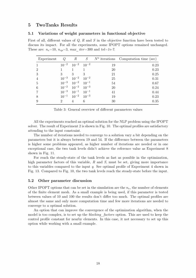
First of all, different values of Q, R and S in the objective function have been tested todiscuss its impact. For all the experiments, some IPOPT options remained unchanged.These are: ne=10, ncp=3, max_iter=300 and tol=1e-7.
Experiment Q R S No iterations Computation time (sec)
Table 3: General overview of different parameters values
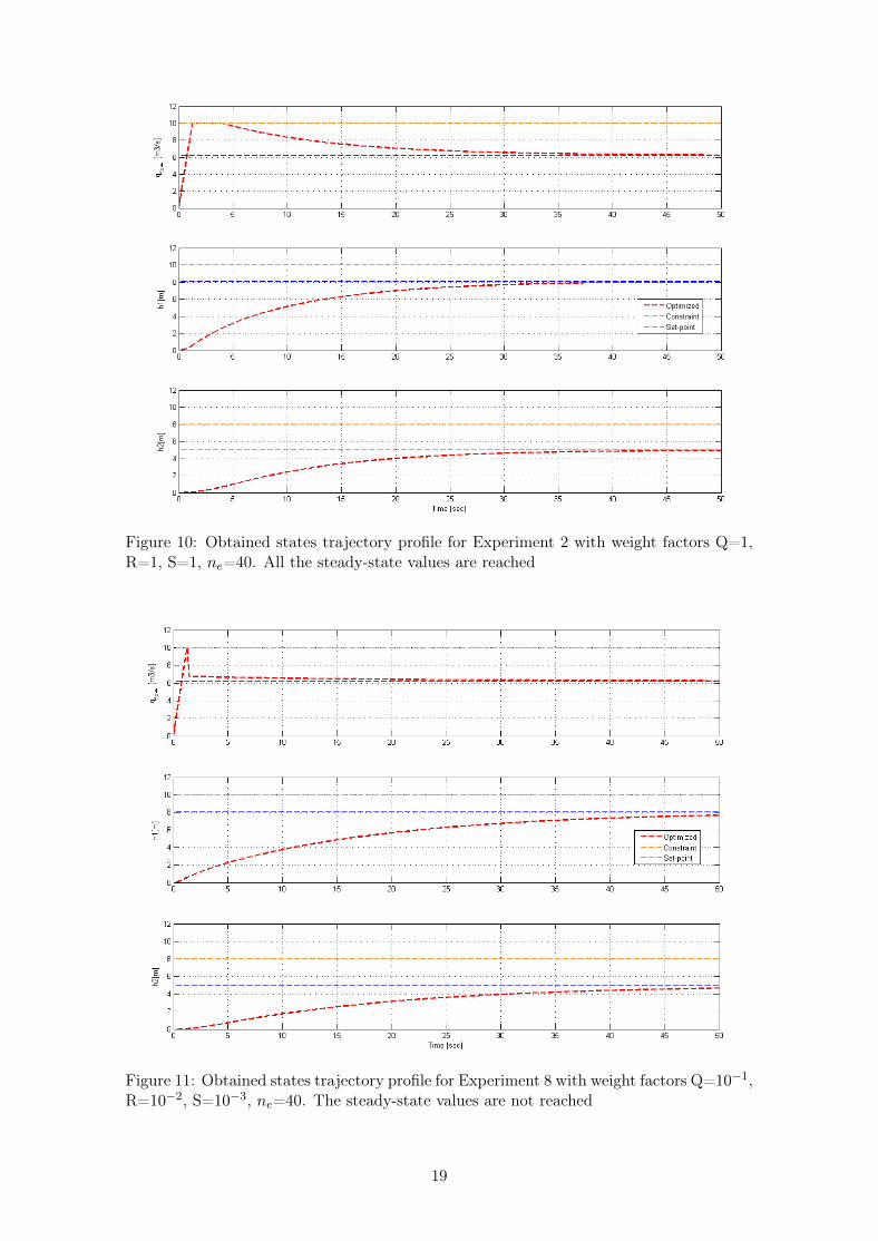
All the experiments reached an optimal solution for the NLP problem using the IPOPTsolver. The result of Experiment 2 is shown in Fig. 10. The optimal profiles are satisfactoryattending to the input constraint.
The number of iterations needed to converge to a solution vary a bit depending on theparameters but it is always between 19 and 54. If the difference between the parametersis higher some problems appeared, as higher number of iterations are needed or in oneexceptional case, the two tank levels didn’t achieve the reference value as Experiment 8shown in Fig. 11.
For reach the steady-state of the tank levels as fast as possible in the optimization,high parameter factors of this variable, R and S, must be set, giving more importanceto this variables compared to the input q. See optimal profile of Experiment 4 shown inFig. 13. Compared to Fig. 10, the two tank levels reach the steady-state before the input.
5.2 Other parameter discussion
Other IPOPT options that can be set in the simulation are the ne, the number of elementsof the finite element mesh. As a small example is being used, if this parameter is testedbetween values of 10 and 100 the results don’t differ too much. The optimal profiles arealmost the same and only more computation time and few more iterations are needed toconverge to a optimal solution.
An option that can improve the convergence of the optimization algorithm, when themodel is too complex, is to set up the blocking_factors option. This are used to keep thecontrol profile constant for nearby elements. In this case, it not necessary to set up thisoption while working with a small example.
18
Figure 10: Obtained states trajectory profile for Experiment 2 with weight factors Q=1,R=1, S=1, ne=40. All the steady-state values are reached
Figure 11: Obtained states trajectory profile for Experiment 8 with weight factors Q=10−1,R=10−2, S=10−3, ne=40. The steady-state values are not reached
19
Another interesting thing is to try to simulate the problem without posing constraint onthe input q(t) from eq. (26). As shown in Fig. 12, a solution is found and the steady-statesare reached but the input goes over 15m3/s.
Figure 12: Obtained states trajectory profile for Experiment 2 without input u(t) con-straint with weight factors Q=1, R=1, S=1, ne=40. The steady-state values are all reached
Figure 13: Obtained states trajectory profile for Experiment 4 with weight factors Q=10−3,R=10−2, S=10−2, ne=40. The steady-state values are reached a bit earlier than with equalparameter values for all the variables.
20
6 Implementation of the Biomass Drum Boiler
After a simple example was given in the previous section in order to illustrate the concept.In this chapter, the optimal start up control problem of the steam boiler case is discussedand implemented. As this model is more complex, Dymola will be used in order to avoidproblems with maximum number of equations. Another reason is because the model hasbeen build with this environment.
Firstly, a basic description of the model is given. Afterwards some notes about themodifications done to the model in order to adapt it for the optimization will be described.
6.1 Model
The drum boiler from [8] is used. Also some information about the start-up optimizationof the drum is followed in [16]. The equations used for this model are described below.
The next global mass balance in the drum boiler is considered:
dm
dt= qm,W − qm,S , (29)
m = ρvVv + ρlVl +mD, (30)
Inside the drum boiler there is liquid water and steam, both are assumed to be atthe phase boundary. Feed water goes into the drum boiler and saturated steam goesout. A furnace modeled with a PrescribedHeatFlow is used to supply energy to heat upand evaporate the water in the rising tubes. In order to describe these properties, thestandard Media Water.IF97 model is used. Unfortunately, this library is not supported bythe JModelica platform. Therefore, another approximation for the water/steam propertiesis used.
The energy balance of the steam boiler is formulated by eq.(31).
dU
dt= qF + qm,Whw − qm,Shs, (31)
U = ρvhvVv + ρlhlVl − p(Vv + Vl) +mDcp,DTD, (32)
The total volume of the drum Vl is given by:
Vt = Vv + Vl, (33)
It is considered that the specific enthalpy of steam that leaves the drum boiler is thesame as the vapor enthalpy:
hs = hv, (34)
Finally, the thermal stress on the boiler is the thick-wall component given by eq.(35).
σD = kdTDdt
, (35)
Once the mathematical formulation describing the boiler’s dynamics is done. Themodel can be implemented in Modelica and simulated in Dymola. The problem appearswhen this model should be optimized. A state-space representation is obtained by ma-nipulating the equations shown above and by combining them. In this case, as suggestedin [8], the pressure p and volume of liquid Vl are used as state variables. For furtherstudy in the model equations transformers, follow [8]. The resulting equations from thistransformation are:
21
e1,1dVldt
+ e1,2dp
dt= qm,W − qm,S , (36)
e2,1dVldt
+ e2,2dp
dt= qF + qm,Whw − qm,Shs, (37)
where
e1,1 = ρl − ρp, (38)
e1,2 = Vv∂ρv∂p
+ Vl∂ρl∂p
, (39)
e2,1 = ρlhl − ρphv, (40)
e2,2 = Vv(hv∂ρv∂p
+ ρv∂hv∂p
) + Vl(hl∂ρl∂p
+ ρl∂hl∂p
)− Vvl +mDcp,D∂Tsat(p)
∂p, (41)
In Listing. 4, the relevant code referring to the equations of the drum boiler is given.1 equation2 // Basic equations3 V = Vl + Vv ;4 der_M = der(Vl ) ∗ sa t . d_ls + Vl∗ sa t . d_d_ls_dp∗der(p)−5 der(Vl ) ∗ sa t . d_vs + Vv∗ sa t . d_d_vs_dp∗der(p) ;6 der_E = der(Vl ) ∗ sa t . d_ls∗ sa t . u_ls+ Vl∗ sa t . d_de_ls_dp∗der(p)−7 der(Vl ) ∗ sa t . d_vs∗ sa t . u_vs+ Vv∗ sa t . d_de_vs_dp∗der(p)−8 40 + Cp ∗ m_t ∗ sa t .d_T_s_dp∗der(p) ;9 // Mass balance
10 der_M = i n l e t .w + ou t l e t .w;11 // Energy balance12 der_E = i n l e t .w∗( i n l e t . h ) + ou t l e t .w∗( ou t l e t . h ) + wal l . Q_flow ;13 // Momentum balance14 i n l e t . p = ou t l e t . p ;15 i n l e t . p = p ;16 p = sat . p ;17 // Boundary conditions18 ou t l e t . h = sat . h_vs ;19 wal l .T = sat .T_s ;20 y=Vl ;21 sigma=60∗ sa t .d_T_s_dp∗der(p) ;
Listing 4: Drum boiler equations in Modelica model
In the drum boiler model the continuous-time states x, controlled inputs u and modeloutputs y are determined below.
To optimize this model a quadratic objective function, constraints and a optimizationinterval are defined. This function is minimized over the optimization interval and somedeviations from the reference state are penalized. In this case, the pressure in the drum
22
Figure 14: Complete system model of the drum boiler in Dymola
boiler Psat and the stream mass flow outside the drum msteam are the ones chosen. Theobjective function with their weighting factors and reference state is
minu(t)
∫ tf
t0
α(Psat − Pref )2 + β(qm − qm,ref )
2dt (42)
where pref=180bar, qm,ref=185kg/s and the weighting values α = 10−3 and β = 10−4.Apart from the objective function, a number of constraints must be satisfied over all
the optimization horizon. These constraints can be divided in input constraints, whichcontrol the bounds, such as:
0 ≤ Qflow ≤ 500MW (43)0 ≤ Yvalve ≤ 1 (44)
In order to avoid big sudden changes, a constraint on the derivative of the heat flow isput.
− 25MW/min ≤dQflow
dt≤ 25MW/min (45)
Other variable start constraints are fixed to assure good profile results. Despite theinitial simulation, the thermal stress is beyond reasonable limits. Therefore, a constraintis imposed to avoid excessive values:
− 10N/mm2 ≤ σD ≤ 10N/mm2 (46)
23
As it’s important to get good reference values, a simulation using a predefined heatflow load is made to check the final state and get reference values. These are then usedto facilitate the solver to converge to a solution. Also, the trajectory from the load willbe taken after to be the initial trajectory in the NLP problem to save some of the timerequired to solve the problem. Otherwise, without an initial trajectory and an initial guess,it is really difficult to find a feasible solution. As seen in Table 1, the option initial_trajis set in order to assure the usage of the simulation result. In this case, the selection ofthe weighting factors is also of importance to get the best result and cannot be chosenarbitrary in the example of the two tanks in series.
6.2.1 Initialization
A first simulation will be done to get the reference values and the initial trajectory of thestate variables. In Listing. 5 the Python script code necessary to compile, build and loadthe simulation is given.
1 # Import l i b r a r y f o r path manipulat ions2 import os . path3
4 # Import the needed JModelica . org Python methods5 from pymodelica import compile_fmu6 from pyfmi import load_fmu7 from pyjmi import get_f i l e s_path8
9
10 ### 1. Compute i n i t i a l guess t r a j e c t o r i e s by means o f s imu la t i on11 # Locate the Modelica and Optimica code12 f i l e_pa th s = ( os . path . j o i n ( get_f i l e s_path ( ) , "DrumBoiler .mo" ) ,13 os . path . j o i n ( get_f i l e s_path ( ) , "DrumBoilerStartup .mop" ) )14
15 # Compile the opt imiza t i on i n i t i a l i z a t i o n model16 init_sim_fmu = compile_fmu ( "DrumBoilerStartup . Startup1Reference " ,17 f i l e_paths , separate_process=True )18
22 # Simulate23 i n i t_r e s = init_sim_model . s imulate ( start_time =0. , f ina l_t ime =3600.)
Listing 5: Python script for simulating the model for an initial guess.
The code in Listing. 5 illustrates how Modelica and Optimica files are located andthen the Optimica optimization class Startup1Reference, where the simulation model iscompiled, loaded and finally simulated.
Once the simulation is done, the results are shown in Fig. 15. With this strategy thestartup takes about 45 minutes and the goal is to reduce the startup time as much aspossible without violating the constraints put.
Now that the initial simulation is done, this data can be used to provide the solverwith a good initial guess. The results of the dynamic optimization are discussed in thenext section.
6.3 Results
The infinite-dimensional optimal control problem given in the previous section is translatedinto a finite dimensional nonlinear programming problem, using a simultaneous collectionmethod implemented in the CasADi package, by approximating both control and stateprofiles with a Lagrange polynomial based on Radau points. This results into a large-scale
24
Figure 15: Simulation of the model with heat flow as a ramp and valve opened
non-linear optimization problem. Algorithm based on Sequential Quadratic Programming(SQP) or interior method, such as IPOPT provides an efficient solution method for theNLP problem. The first and second derivatives, as well as the sensitivity informationrequired by IPOPT are automatically generated by CasADi.In this thesis, the software used is JModelica v.1.14 as well as IPOPT v.3.8.11 runningwith the linear MA57 solver, which performs better than the standard MUMPS solver,have been selected. The optimization time interval is set to one hour. The PC used isan Intel Core i5-3210M, 2.5 GHz, with 8GB RAM. Last but not least, the simulationtrajectories were used to provide a good initial guess for the solver. Table 4 shows someresults after NLP problem solving using the JModelica framework.The obtained optimized trajectories are illustrated in Fig. 16. The figures clearly showthat by solving the start-up problem as an OCP, the steam production is achieved withina shorter time to fulfil turbine inlet parameters, compared to classical start-up strategy,and without violating the imposed hard-constraint on the thermal-stress of thick-walledcomponent, which increases its lifetime consumption.
Table 4: Execution and NLP function evaluation timesvalue unit
Nr. of variables 7595 [-]Nr. of objective function evaluation 1090 [-]Nr. of Lagrange Hessian evaluation 290 [-]NLP function evaluations time 1.96 [sec]Initialization time 1.25 [sec]Solution time 7.01 [sec]Total time 8.27 [sec]
25
Figure 16: Optimal control profile of the dynamic optimization problem with t=3600sec
Fig. 16 shows the results of the dynamic optimization problem. With this configuration,the startup time is reduced to 30 minutes without violating any of the constraints imposed.As expected, the valve opening is completely opened during almost all the optimizationinterval. Compared to the profiles from [16], the similarities are visible.
When the number of finite elements are modified, the optimization profiles remain thesame, as well as the minimized cost function value. The main difference when putting ahigher number of finite elements is the higher number of the iterations needed. More timeis also needed for the solver to converge to a optimal solution.
Fig. 17 shows the difference between the startup with the predefined inputs in greenand the optimized curves in red. The reference values are achieved.
26
Figure 17: Comparison between the initial simulation and the optimized curves
27
7 Discussion and Conclusions
7.1 Optimization results
The results obtained from the two tanks in series were as expected.The goal of this basicexample was to familiarize with the JModelica framework and Optimica extension beforetackling a more complex case. For that reason, it was not necessary to test the CasADipackage and the JMUModel was used instead. It is also really interesting to test the differentoptions available in both JModelica.org and IPOPT which makes the difference whensolving the NLP problem. Thanks to this example, where it was demonstrated that withJModelica.org platform the models can be implemented with less effort and knowledgein programming, which makes it more accessible for more people in the industrial andscientific community. The differences are visible compared to [11], where a long pure C++code is used to implement the same example.
Referring to the drum boiler startup, which was the main goal in the thesis, the im-plementation was a bit more difficult due to the complexity of the model and the use ofsome constraints. One of the main problems was to approximate the water media modelwhich is essential when simulating and optimizing this model.
The results obtained are satisfactory, despite it was not possible to realize the minimumtime problem as it was impossible for the solver to find an optimal solution. The parameterand weight factors were chosen as similar as possible to [16], in order to compare theresults with this study and demonstrate the advantages in comparison to the JModelica.orgplatform.
Before implementing the examples, a study of the NMPC theory was necessary tochoose a better strategy suited to the goals of this thesis and to discover the differentsteps needed to implement an NMPC.
7.2 Further work
This thesis has shown how Modelica models can be interfaced with JModelica.org platformin order to optimize a ateam boiler process. As it was only a small part taking part ina bigger process, much more work can be done to implement more processes. It will beinteresting to enlarge the drum boiler model with the model presented in [8], that includea more approximated behavior of the real process. The big problem in this thesis wasto find an acceptable approximation of the water media model which can be improved infuture works.
A good configuration of the optimization options as well as Optimica constraints wereneeded for the IPOPT solver to converge to a solution. It will be also interesting to useother solvers to see the influence of the solver choice.
When models are too complex can be also interesting to investigate the use of theJModelica option blocking_factors, which can help the user to converge to an optimalsolution when the solver is not able to found any.
7.3 Facilities and experience with JModelica
The JModelica.org platform is an exceptional tool when optimizing dynamic models. Itwill be good if more documentation and examples were introduced as this framework offersa wide range of possibilities to adapt the options according to the goals of each model.Another recently improvement is the addition of the CasADi package, which makes thistool more efficient when solving a large NLP problem. The main issue of this frameworkis the poor integration of the Modelica fluid library which hopefully will be integrated andimproved in future actualizations. Another thing to improve is the lack of information
28
when errors appear when compiling or running a model. Despite all this inconveniences, alot of effort has been put in this platform to make it suitable for a wider number of people.
29
References
[1] J. Aburajabaltamimi. Development of Efficient Algorithms for Model Predictive Con-trol of Fast Systems. Fortschritt-Berichte VDI: Reihe 3, Verfahrenstechnik. VDI-Verlag, 2011.
[2] J. Åkesson. “Optimica—An Extension of Modelica Supporting Dynamic Optimiza-tion”. eng. In: Bielefeld, Germany, 2008.
[3] J. Åkesson et al. “Modeling and Optimization with Modelica and Optimica Usingthe JModelica.org Open Source Platform”. In: Proceedings of the 7th InternationalModelica Conference 2009. Modelica Association, 2009.
[4] J. Åkesson et al. “Modeling and Optimization with Optimica and JModelica.org—Languages and Tools for Solving Large-Scale Dynamic Optimization Problems”. In:Computers and Chemical Engineering 34.11 (2010), pp. 1737–1749.
[5] E. Andersson. “Development of a dynamic model for start-up optimization of coal-fiered power plants”. Master’s Degree Project. KTH Electrical Engineering.
[6] J. Andersson. “A General-Purpose Software Framework for Dynamic Optimization”.PhD thesis. Department of Electrical Engineering (ESAT/SCD) and Optimizationin Engineering Center, Kasteelpark Arenberg 10, 3001-Heverlee, Belgium: ArenbergDoctoral School, KU Leuven, 2013.
[7] J. Andersson et al. “Integration of CasADi and JModelica.org”. In: 8th InternationalModelica Conference 2011. Dresden, Germany, 2011.
[8] K. Åström and R. Bell. “Drum-boiler dynamics”. In: Automatica 36.3 (2000), pp. 363–378.
[9] B. W. Bequette. Process control: modeling, design, and simulation. Prentice HallProfessional, 2003.
[10] L. Biegler. Nonlinear Programming: Concepts, Algorithms, and Applications to Chem-ical Processes. MOS-SIAM Series on Optimization. 2010. isbn: 9780898719383.
[11] C. Carbonell Buqueras. “Model Based Predictive Control using Modelica and opensource components”. Master’s Degree Project. Norwegian University of Science andTechnology.
[12] F. Casella, F. Donida, and J. Åkesson. “Object-Oriented Modeling and OptimalControl: A Case Study in Power Plant Start-Up”. In: 18th IFAC World Congress.Milano, Italy, 2011.
[13] Dassault Systemès. Dassault Systemès Home Page. url: http://www.3ds.com/products - services/ catia / capabilities / systems - engineering / modelica -systems-simulation/dymola (visited on 04/24/2014).
[14] M. Diehl. Numerical Optimal Control. 2011.
[15] R. Findeisen and F. Allgöwer. “An Introduction to Nonlinear Model Predictive”. In:Control, 21st Benelux Meeting on Systems and Control, Veidhoven. 2002, pp. 1–23.
[16] R. Franke, M. Rode, and K. Krüger. “On-line Optimization of Drum Boiler Startup”.In: Proceedings of the 3rd International Modelica Conference. 2003, pp. 287–296.
[17] R. Franke and L. Vogelbacher. “Nonlinear Model Predictive Control for Cost Op-timal Startup of Steam Power Plants (Nichtlineare modellprädiktive Regelung zumkostenoptimalen Anfahren von Dampfkraftwerken)”. In: at–Automatisierungstechnik54.12 (2006), pp. 630–637.
[18] P. Fritzson. Principles of object-oriented modeling and simulation with Modelica 2.1.John Wiley & Sons, 2010.
[19] D. E. Kirk. Optimal control theory: an introduction. Courier Dover Publications,2012.
[20] K. Krüger, R. Franke, and M. Rode. “Optimization of boiler start-up using a non-linear boiler model and hard constraints”. In: Energy 29.12âĂŞ15 (2004), pp. 2239–2251.
[21] F. Magnusson. Collocation methods in JModelica.org. Master’s Thesis. Departmentof Automatic Control, Lund University, Sweden, 2012.
[22] J. Nocedal and S. J. Wright. Numerical Optimization. 2nd. Springer, 2006.
[23] OpenModelica. OpenModelica Home Page. url: http://www.openmodelica.org(visited on 04/15/2014).
[24] J. Rantil et al. “Multiple-Shooting Optimization using the JModelica.org Platform”.In: 7th International Modelica Conference 2009. Como, Italy, 2009.
[25] The Modelica Association. The Modelica Association Home Page. 2014. url: http://www.modelica.org (visited on 04/20/2014).
[26] The Science and Technology Facilities Council. HSL for IPOPT. 2014. url: http://www.hsl.rl.ac.uk/ipopt/ (visited on 05/08/2014).
[27] A. Wächter and L. T. Biegler. “On the implementation of an interior-point filter line-search algorithm for large-scale nonlinear programming”. English. In: MathematicalProgramming 106.1 (2006), pp. 25–57.