School of Education, Culture and CommunicationDivision of Applied Mathematics

BACHELOR THESIS IN MATHEMATICS / APPLIED MATHEMATICS

Lattice approximations for Black-Scholes type models in Option Pricing

by

Anne Karlén and Hossein Nohrouzian

Kandidatarbete i matematik / tillämpad matematik

DIVISION OF APPLIED MATHEMATICS

MÄLARDALEN UNIVERSITY

SE-721 23 VÄSTERÅS, SWEDEN

School of Education, Culture and CommunicationDivision of Applied Mathematics

Bachelor thesis in mathematics / applied mathematics

Date:

2013-06-05

Project name:

Lattice approximations for Black-Scholes type models in Option Pricing

Authors:

Anne Karlén and Hossein Nohrouzian

Supervisor:

Professor Sergei Silvestrov

Examiner:

Anatoliy Malyarenko

Special thanks to:

Anatoliy Malyarenko, Jan Röman and Karl Lundengård

Comprising:

15 ECTS credits

The first named author of this thesis has written and is responsible for Sections 2.7, 2.8 , 2.9and the whole Chapter 5. The second named author has written and is responsible for the restof Chapter 2, the whole Chapters 3, and Chapter 4, and the appendix. All the remaining partsof this thesis were written by the two authors together.

Abstract

This thesis studies binomial and trinomial lattice approximations in Black-Scholes type optionpricing models. Also, it covers the basics of these models, derivations of model parameters byseveral methods under different kinds of distributions. Furthermore, the convergence of bino-mial model to normal distribution, Geometric Brownian Motion and Black-Scholes model isdiscussed. Finally, the connections and interrelations between discrete random variables underthe Lattice approach and continuous random variables under models which follow GeometricBrownian Motion are discussed, compared and contrasted.

Contents

1 Introduction 4

2 Binomial Model 82.1 Payoff to European and American Options . . . . . . . . . . . . . . . . . . . 82.2 Binomial Expansion . . . . . . . . . . . . . . . . . . . . . . . . . . . . . . . 102.3 Calculating the Price of European Options . . . . . . . . . . . . . . . . . . . 122.4 Calculating the Price of American Options . . . . . . . . . . . . . . . . . . . 122.5 Risk-Neutral Probability (The Cox-Ross-Rubinstein Model) . . . . . . . . . 132.6 Volatility with u and d factors . . . . . . . . . . . . . . . . . . . . . . . . . . 152.7 Random Walks . . . . . . . . . . . . . . . . . . . . . . . . . . . . . . . . . 202.8 Pricing the option . . . . . . . . . . . . . . . . . . . . . . . . . . . . . . . . 232.9 Examples . . . . . . . . . . . . . . . . . . . . . . . . . . . . . . . . . . . . 24

3 Convergence of binomial model to Geometric Brownian motion 283.1 Introduction and Background . . . . . . . . . . . . . . . . . . . . . . . . . . 283.2 The sequence of the binomial models and its convergence to Geometric Brownian

Motion . . . . . . . . . . . . . . . . . . . . . . . . . . . . . . . . . . . . . . 303.3 The sequence of binomial models and its convergence to Black-Scholes model

under risk-neutral probability . . . . . . . . . . . . . . . . . . . . . . . . . . 313.4 Mean and variance of a random variable which is log-normally distributed . . 34

4 Different approaches on Binomial Models 384.1 Random variable Y = ln

(Si+1Si

)is normally distributed . . . . . . . . . . . . 39

4.1.1 Introducing the third equation by p = 1/2 . . . . . . . . . . . . . . . 404.1.2 Introducing the third equation by ud = 1 . . . . . . . . . . . . . . . . 40

4.2 Random variable X = Si+1Si

is log-normally distributed . . . . . . . . . . . . . 434.2.1 Introducing the third equation by p = 1/2 . . . . . . . . . . . . . . . 434.2.2 Introducing the third equation by ud = 1 . . . . . . . . . . . . . . . . 44

4.3 The Jarrow-Rudd model . . . . . . . . . . . . . . . . . . . . . . . . . . . . 454.4 The Tian model . . . . . . . . . . . . . . . . . . . . . . . . . . . . . . . . . 464.5 The Trigeorgis model . . . . . . . . . . . . . . . . . . . . . . . . . . . . . . 484.6 The Leisen-Reimer model . . . . . . . . . . . . . . . . . . . . . . . . . . . 49

2

5 Trinomial Model 515.1 Properties of the trinomial distribution . . . . . . . . . . . . . . . . . . . . . 52

5.1.1 A stretch to the multinomial distribution . . . . . . . . . . . . . . . . 525.2 Boyle’s approach of deriving probabilities . . . . . . . . . . . . . . . . . . . 535.3 The replicating portfolio in the trinomial model . . . . . . . . . . . . . . . . 555.4 Trinomial probability under lognormal transformation . . . . . . . . . . . . . 585.5 Explicit finite difference approach . . . . . . . . . . . . . . . . . . . . . . . 595.6 The case of binomial and trinomial equivalence . . . . . . . . . . . . . . . . 635.7 More on the connection between binomial and trinomial trees . . . . . . . . . 67

6 Conclusion 696.1 Summary of reflection of objectives in the thesis . . . . . . . . . . . . . . . . 71

6.1.1 Objective 1 - Knowledge and understanding . . . . . . . . . . . . . . 716.1.2 Objective 2 - Ability to search, collect, evaluate and interpret . . . . . 726.1.3 Objective 3 - Identify, formulate and solve problems . . . . . . . . . 726.1.4 Objective 4 - Communication of our project to different groups . . . . 726.1.5 Objective 5 - Ability to put our work into a societal context and its

value within it . . . . . . . . . . . . . . . . . . . . . . . . . . . . . 73

A Appendix 76A.1 Black-Scholes PDE . . . . . . . . . . . . . . . . . . . . . . . . . . . . . . . 76A.2 Black-Scholes formula for European Call option . . . . . . . . . . . . . . . . 78

3

Chapter 1

Introduction

Investing in the market always contains some risk. People invest some of their capital in themarket with the aim of obtaining maximum profit at minimum possible risk. There are differ-ent levels of risk aversion. People who want to do some business in the future and are afraidof loosing money due to changed conditions (e.g. increased price of raw material or unfavor-able exchange rates), might want to secure themselves through hedging (eliminating the risk).That can be obtained with the purchase of options. An option is a contract which states that theholder of the option is allowed to buy (or sell) a certain asset at a predetermined price at prede-termined date(s). Buying options seems to be a secure way of investing in the market. But arethey always profitable? No. This would mean arbitrage opportunities (free lunches) and con-sequently everyone would invest in them. The question is how these options should be pricedin order to avoid arbitrage opportunities, i.e., the possibility to earn profit without risk. Fromthe course Introduction to financial mathematics we already knew that there exist formulasfor fair option pricing, but the parameters were always given to us when we were supposed touse these formulas. The question arose how the parameters actually are determined and whenwe discovered that there are many different papers concerning option pricing and derivationof parameters, and that different papers present different results, the idea for the topic of ourthesis was born. The problem is that there are unpredictable factors, namely the evolution ofthe price of the underlying asset and the probability of attaining these prices. The price can goup or down, but by how much? And what is the probability to move in either direction? It isnot totally reasonable to assume that the probability is 50% each. Additionally there could beno price change at all, so we have a third possibility for the evolution of the price. Intuitivelywe would expect the probability of no price change to be smaller than the probabilities of upand downward movements. So unpredictable parameters such as random variables or even astochastic process are involved in option pricing and therefore it is a complex and complicatedfield to examine.

Option pricing is a part of financial analysis which deals with different areas of mathematicssuch as probability, stochastic processes, ordinary differential equations and stochastic differ-ential equations. So how do we compute the fair price for an option? Well, first of all thereare different kinds of options in the market which are constructed differently. However, there

4

is a common algorithm for calculating the fair price of any option and this algorithm statesthat the fair price of an option is its discounted expected payoff. When we talk about expectedvalue in simple cases, we know that it is the average or mean of a sample or population. Butfinding expected values of some processes is not that easy. Moreover there are some contro-versial questions. How to calculate this expected value? Is it always possible to calculate theprice of an option analytically? How should one translate mathematical formulas to computerlanguage? If it is not possible to calculate the price of an option analytically, which numericalmethod should be used to estimate the price of the option? What is the error of estimations?What are the definitions for different options and how does one calculate their payoffs? Toanswer some of these questions, we will try to explain the basic definitions and ideas aboutoptions and how to price them. This process is strongly related to our knowledge which wehave obtained by studying the Bachelor’s Program in Analytical Finance at Mälardalen Hög-skola. We will go through the basic ideas which are vital for understanding the algorithm ofpricing options specifically in computer language and when we talk about simulating someprocess for which we can find the result by numerical methods [6].

After our introduction, we will in Chapter 2 go through the concept of binomial models. Wewill study how it is possible to price an option using a binomial tree. In the binomial modelChapter, we will start with the definitions of payoff for European and American options [7],which we have studied in the course "Introduction to Financial Mathematics". After that, wewill follow our process by studying some probability theorems and definitions [21] which areessential for getting a good understanding for pricing options via the binomial model approach.We obtained this knowledge in our "Probability" course. Then, using binomial approach, wewill try to explain how the price of American and European options can be calculated. At thisstep, we will be able to analyze a binomial tree and we will have a system of equations withsome unknowns. We will continue our process by calculating them. Firstly, we will try tofind the value for risk-neutral probability [4], [7] by constructing a replicating portfolio. Herewe will get help from different literature like our knowledge from the courses "StochasticProcesses" [12] and its lecture notes [14]. Secondly, we will derive the other unknowns inour system of equations, namely up and down factors in full details and we will study theCRR model (Cox, Ross and Rubinstein model) and its results [4]. After that, we will talkabout random walks and transition probabilities which will help us to derive the backward andforward equations for pricing options [12],[14]. Consequently, we will discuss the formula forpricing the option [7]. Finally, we will end Chapter 2, with some example which will showhow our process can be helpful to price options, especially when we deal with an AmericanPut option, in which early exercise on a predetermined date is possible.

In Chapter 3, we start to compare and contrast the behavior of a random variable, namelystock price, in discrete and continuous time. Additionally, we will consider the result of Blackand Scholes [1] and Merton [15]. We know they assumed that the dynamic of risky securityprices follows a Geometric Brownian Motion. We will also follow Cox, Ross and Rubinstein[4] approach to see how as well the sequence of the binomial model converges to Geometric

5

Brownian Motion. To do so, we will start studying the sequence of the binomial model andits convergence to normal distribution [12],[14],[21]. Then we will show how the sequenceof the binomial model converges to the Black-Scholes model under risk neutral probability[12],[14]. After that, we will make a distinction between normal and log-normal randomvariables. Moreover, we will discuss how stock prices can be treated as log-normal randomvariables with normal-distribution and how it can be treated as a normal random variable withlog-normal distribution. In this part we do some interesting derivations using our knowledgefrom calculus and probability [21], which are really useful for approximation of some variantsof binomial models to the Black-Scholes pricing formula.

In Chapter 4, we will study some different variants of binomial models. We have seen theresult and formula for some of these variants in our course "Analtical Finance I" [17], butwe will try to apply our knowledge to derive the final formulas in details. We will see thatfor the binomial approach, we will always have two equations for expected value and variancewhich, depending on our choice of normality or log-normality of our random variable (namelystock price), can be approximated differently with different means and variances. Moreover,we will see that we have a system of two equations and three unknowns. We will see thatfor example Cox, Ross and Rubinstein [4] chose their third equation like ud = 1. In simplecases, we introduce our third equation by ud = 1 or p = 1/2 and we will approximate thebinomial model in a way that the mean and the variance of our models converge to the Black-Scholes formula. Then we will study some other models like Jarrow-Rudd model [10],[9],Tian model [19], Trigeorgis model [20] and Leisen-Reimer model [13]. We will see how theapproximation of these different models works and what advantage and disadvantage eachmodel has. There are lots of other models which can be considered, but we will finish thischapter by just considering the models that we have mentioned.

In Chapter 5, we will study the trinomial model. We start off with the basic principles ofthe trinomial distribution. It is similar to the binomial distribution, but not as widely used.Consequently there was less literature available that covered the subject but due to the simil-arity with the binomial model, previous knowledge of probability theory and Wackerly [21],the concept and properties of trinomial distribution is derived and explained. It is importantso that further parts can be understood.

Directly after the basics of trinomial distribution we study the paper of Boyle from 1988 [2]because it extends Cox, Ross and Rubinstein approach of risk neutral valuation with jumps intwo directions (binomial model) into a model with jumps in three directions (trinomial model)with the condition of risk neutral return which in the short term is the risk free interest rate.The probabilities under this process are derived connecting mean and variance of discreteand continuous distributions where the discrete functions are approximations of the lognormaldistribution of the underlying asset which is governed by a Geometric Brownian Motion. Thismodel will show that we have two constraints and five unknown parameters, giving no uniqueparameters for the probabilities.

6

The next section deals with risk neutral probability as well. We will examine if the replicatingportfolio can generate the contingent claim if three different movements on the underlyingasset are assumed (in contrast to two, which we examine in the binomial lattice). Since we usedKijima [12] and the lecture notes from Stochastic Processes [14] for the replicating portfolioin the binomial model, we find it appropriate to use it for the trinomial variant as well.

Another method for finding parameters suitable to generate contingent claims was establishedby Kamrad and Ritchken in 1991 [11]. Their idea was to approximate the logarithm of therandom variable that describes the return of the underlying asset in one time step. Even herethe random variable is discretized in the trinomial lattice and the first two moments of thecontinuous distribution is matched with those of the discrete distribution.

As we have seen we show several methods where the approximation of the continuous randomvariable is done by a lattice approach. The next part however uses another method, namely theexplicit finite difference approach. We show how the partial derivatives in the Black-Scholesformula can be discretized and further processed in order to find probability densities thatsatisfy the partial differential equation. Originally Brennan and Schwartz [3] developed thistechnique, but we studied the notes from Analytical Finance [17] and Hull [7] as well, becausethe paper itself is structured in a complicated way. For easier understanding we even includedgraphics in this part.

In the last part we try to find a connection between binomial and trinomial trees based onan observation of one of the authors of this thesis that binomial lattices and trinomial latticesoverlap. As we investigated this connection further we found a paper by Derman et al from1996 [5] which was really helpful and led to yet another discovery, namely that there are treemodels with constant volatility, called standard trees, and trees that are constructed in orderto match the volatility smile with varying volatility, called implied trees. We give a briefexplanation of this detection.

We found it reasonable as well to show the Black-Scholes formula and how it is derived. Theappendix covers this subject.

All sources that we have used are either published papers or text books, or lecture notes fromprofessors at Mälardalens Högskola. We had the great opportunity to download the papersfrom Jstor through our university accounts. We find all references very reliable since they areprovided through academic sources and have educated many students and people working infinance and economics, before us.

7

Chapter 2

Binomial Model

In market the price of stocks move randomly. The price of stocks can go up, down or remainconstant between two time intervals. So, the movements of stock prices are stochastic pro-cesses. In simple case we can consider a random walk with predefined length of movements.We assume the price of stock can go up or down for a certain amount in each time intervalwith the probability of p and 1− p respectively. This simple model is called Binomial model.The price of stock at time zero is denoted by S0 and it is usual to denote the amount of in-creasing by uS0 and the amount of decreasing by dS0. One can start from today, i.e., node oneat the time zero and build a binomial tree for a finite time interval. Figure 2.1 illustrates threesteps binomial tree graphically. It is obvious that the possible stock prices can be calculatedeasily at any node. But, how to calculate the fair price of an option? As mentioned before thediscounted expected payoff must be considered. In binomial tree at any node we can count allthe possible paths to reach that specific node. And then we can formulate our expected payoff.Instead of counting all possible way to reach a specific node we need to explain the formu-lation of binomial expansion and binomial coefficient which can represent the probability ofreaching at any specific node at any step. But, first let start by the most important definitionsfor option pricing and then we will continue by some probability theorems and definitions aswell as binomial expansion.

2.1 Payoff to European and American Options

Let us start with the definition of American and European options1 [7].

Definition 2.1.1. European Options are options which give the holder of the options the right,but not the obligation, to exercise them at maturity.

1In the market there exist several different kinds of options, like Bermudan Options, which are a part ofnonstandard American options, Asian options, Currency Options, Swap Options, Barrier Options and ... [7]

8

S0

S0u

S0d

S0u2

S0ud

S0d2

S0u3

S0u2d

S0ud2

S0d3

∆T

∆t ∆t ∆t

t0 t1 t2 T

Figure 2.1: Three Steps Binomial Tree

Definition 2.1.2. American Options are options which give the holder of the options the right,but not obligation, to exercise them at any time up to maturity.

It can be proved that the price of an American put option must be greater or or equal to theprice of a European put option [7]. It can also be proved that the price of American call andEuropean call options is the same [7] under the condition that the underlying asset does notpay dividends. As it was explained, the honest price for an option is its discounted expectedpayoff. For discounting a price it is common to use the risk-free interest rate r with continuouscompounding. To explain it mathematically we can write:

Price = e−r∆T E[payoff] (2.1)

To distinguish between the options we can define their payoffs as follow [7]:

Long Call:

payoff = max{ST −K,0}Short Call:

payoff =−max{ST −K,0}Long Put:

payoff = max{K−ST ,0}

9

f0

fu

fd

fu2

fud

fd2

fu3

fu2d

fud2

fd3∆t ∆t ∆t

t0 t1 t2 T

Figure 2.2: Three Steps Binomial Tree

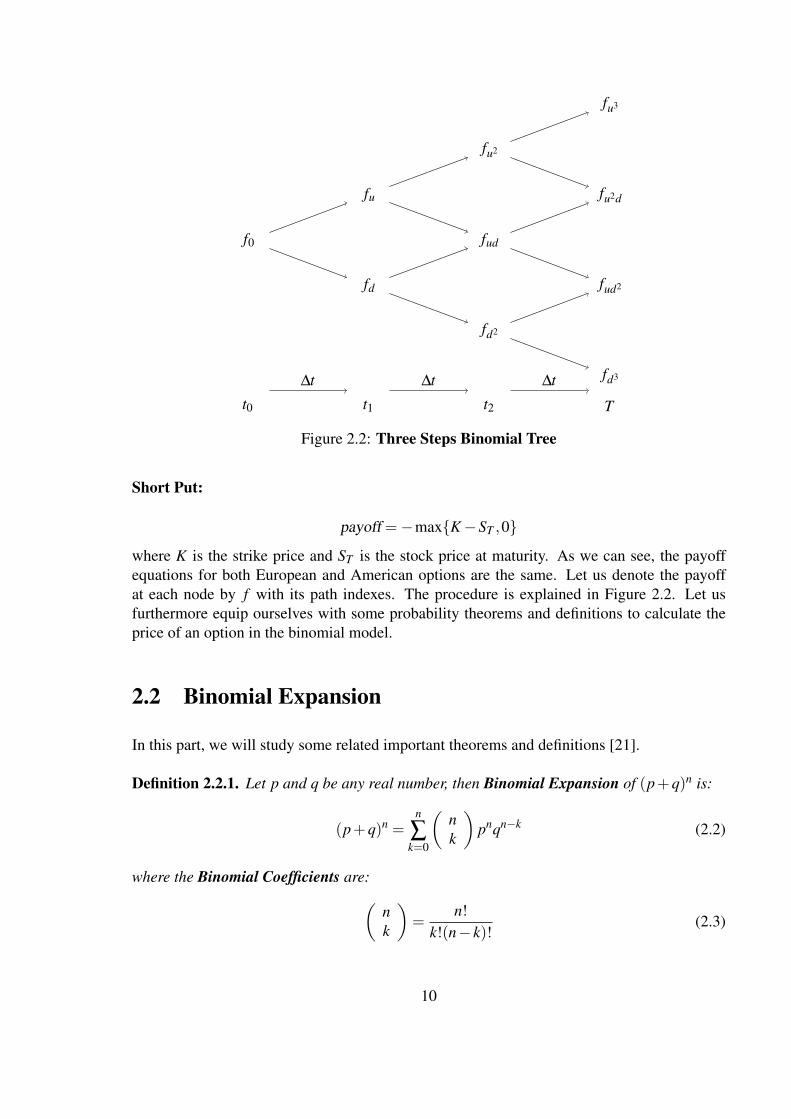
Short Put:

payoff =−max{K−ST ,0}

where K is the strike price and ST is the stock price at maturity. As we can see, the payoffequations for both European and American options are the same. Let us denote the payoffat each node by f with its path indexes. The procedure is explained in Figure 2.2. Let usfurthermore equip ourselves with some probability theorems and definitions to calculate theprice of an option in the binomial model.

2.2 Binomial Expansion

In this part, we will study some related important theorems and definitions [21].

Definition 2.2.1. Let p and q be any real number, then Binomial Expansion of (p+q)n is:

(p+q)n =n

∑k=0

(nk

)pnqn−k (2.2)

where the Binomial Coefficients are:(nk

)=

n!k!(n− k)!

(2.3)

10

The binomial coefficients are useful for calculating the probability distribution in a binomialtree. Let us continue with the next theorem [21].

Theorem 2.2.1. For any discrete probability distribution, the following must be true:1. 0≤ p(y)≤ 1 , for all y2. ∑y p(y) = 1 , where the summation is over all values of y with nonzero probability.

The definition for binomial distribution is [21]:

Definition 2.2.2. A random variable K is said to have a Binomial Distribution based on ntrails with success probability p if and only if

p(k) =(

nk

)pn(1− p)n−k (2.4)

where

k = 0,1,2, ...,n and 0≤ p≤ 1

The formula (2.4) defines the probability function for a discrete random variable. ConsideringTheorem 2.2.1 we say q = 1− p and we will use it to calculate the price of some options.2

Moreover, the following definition will help us to calculate the mean or expected value of adiscrete random variable [21].

Definition 2.2.3. Let Y be a discrete random variable with probability function p(y). Thenthe Expected Value of Y , E(Y ), is defined to be

E(Y ) = ∑y

yp(y) (2.5)

if the above series is absolutely convergent.

Finally, we can find the variance of a discrete random variable using the following theorem[21].

Theorem 2.2.2. Let Y be a discrete random variable with probability function p(y) and meanE(Y ) = µ; then

V (Y ) = σ2 = E

[(Y −µ)2

]= E

(Y 2)−µ

2 (2.6)

Remark 2.2.1. Using Definition 2.2.3 we can see that E(Y 2)= ∑y y2 p(y).

These theorems and definitions will play a considerable role in lattice approaches.

2The mean in the discrete binomial distribution is µ = np and the variance is σ2 = np(1− p) [21].

11

2.3 Calculating the Price of European Options

As we saw, European options can be exercised only at maturity. Since we know the strikeprice it is obvious that we can calculate the pay-off when the stock price is known at maturity.Moreover, we can calculate the probability distribution by (2.4) and the expected value by(2.5). Let us consider the Three Step Binomial Tree in Figure 2.1 and Figure 2.2, and see howit works for a European call option.First, we have a three-step binomial tree. So the binomial expansion is:

(p+q)3 =3

∑k=0

(nk

)pnqn−k = p3 +3p2q+3pq2 +q3

where q = 1− p. And the price of European call option can be calculated by

CE = e−rT [p3 fu3 +3p2q fu2d +3pq2 fud2 +q3 fd3]

Where C is an abbreviation for the price of a European call option and fumdn−m represents thepayoff at any node. Here, m denotes the number of upward movements and n stands for thenumber of steps in our binomial tree. For example when we have three steps in the binomialtree, i.e., n = 3, we have two upward movements, i.e., m = 2, and we can say that the payoffat node u2d is:

fu2d = max{S0u2d−K,0}

Remark 2.3.1. Notice that it is possible to do a backward approach to find the price for aEuropean option, but it can be proved that the result will be the same. We will show thatin Section 2.9. We will also consider the backward approach for calculating the price of anAmerican put option.

2.4 Calculating the Price of American Options

As it was mentioned before, with American options the holder of an option has the right, butnot the obligation, to exercise the option at any time up to maturity. Considering this fact,we can calculate the fair price of an American option. It is really important to calculate thediscounted expected payoff at any possible time for exercising. Let us consider the three-stepbinomial tree. The holder of an American, say put option, has the right to exercise her optionat times t1, t2 or T . The question is when the optimal time to exercise that American putoption is. Let us do it step by step. At time T we know the payoffs. Using that knowledge,it is possible to go one step back on the nodes, which in our example is time t2. Now, wehave to consider every single node as a one step binomial tree and find the optimum payoff.Considering Figure 2.2 we can formulate the explanation above in mathematical language asfollows.

12

optimal{ fu2}= max{

fu2,e−r∆t [p fu3 +(1− p) fu2d]}

= max{(K−ST ,0),e−r∆t [p fu3 +(1− p) fu2d]

}optimal{ fud}= max

{fud,e−r∆t [p fu2d +(1− p) fud2]

}= max

{(K−ST ,0),e−r∆t [p fu2d +(1− p) fud2]

}If we continue doing so, we will be able to calculate the optimal values in all nodes and go backone more time. Then we will use the optimal values of the previous nodes to calculate theirdiscounted expected payoff. We continue doing so until we reach time zero. The discountedexpected payoff at time zero will be the fair price of the American option.

PA = e−r∆t [p×optimal{ fu}+q×optimal{ fd}]Now we almost cover every important aspect of the binomial tree. But we still need to knowmore about the probability p and the u and d factors.

2.5 Risk-Neutral Probability (The Cox-Ross-Rubinstein Model)

Consider a financial market containing of two different securities, a deterministic bond and astock which follows a stochastic process.We assume that the market is free of arbitrage. It ispossible to prove that the stock price is its discounted expected payoff [7],[17].In general:

S(t) = e−rT E p∗[S(T )]

where p∗ is called the Risk-Neutral Probability measure or the equivalent martingale measure.Risk-neutral probability measure in the binomial model was originally calculated by Cox,Ross and Rubinstein. They calculated p∗ as [4]:

p∗ =er∆t−du−d

(2.7)

where u and d are up and down factors in the binomial tree, r is the risk-free interest rate and∆t is the time between each two steps in the binomial tree.Using Definition 2.2.3 and (2.5) the expected stock price in the two step-Binomial tree at timeT can be calculated as [7]:

E[S(T )] = p∗S0u+(1− p∗)S0d (2.8)

E[S(T )] = p∗S0(u−d)+S0d (2.9)

Substituting (2.7) in (2.9) we will get:

E[(S(T )] = S0erT ⇒ S0 = e−rT E[S(T )] (2.10)

The current result tells us that in a risk neutral world, the expected return on a stock is equalto the risk-free interest rate.

13

Calculating Risk-Neutral Probability p∗

Consider a market which consists of two types of financial instruments, bonds and stocks.Moreover, there is no possibility of arbitrage. We know that bonds guarantee a certain amountof profit in a specific time period, but the return on the stock is a stochastic process. To beginwith, we can write the process of these two securities in mathematical language as follows[12],[14],[17]:

B(t) ={

er∆t = 1 ,for t = t0 = 0er∆t ,for t = t1 = T

B represents bonds with deterministic processes and their value at time zero will be one unitof amount of money. At time T it will be their initial value plus the risk-free interest ratecontinuous compounded and 0≤ t ≤ T .As we discussed it previously, stocks follow a stochastic process and this will be as fol-lows:

S(t) ={

S0 ,for t = 0S(T ) ,for t = T

Before going further, it might be crucial to explain our portfolio. Our portfolio is simply ourproperties. We have invested our money in two categories: stocks and bonds. Let us saythat we have decided to invest x percent of our money in bonds and y percent of our moneyin stocks. x and y can get negative values since its possible to short one of the securities tolong the other, but under condition x+ y = 1. Let us call our portfolio h. So the value of ourportfolio at time t is:

V (t,h) = xB(t)+ yS(t)

which represents the value process of portfolio h. We can expand the expected value of theportfolio of bonds and stocks at time t:

E[V (t,h)] ={

xB(0)+ yS(0) ,for t = 0xB(T )+ yE[S(T )] ,for t = T

which can be simplified as:

E[V (t,h)] ={

x+ yS0 ,for t = 0xer∆t + yE[S(T )] ,for t = T

We have already discussed the possible outcomes of S(t) in the one step binomial model. Sothe value process at time t = T can be rewritten as:

V (t,h) ={

xer∆t + yS0u ,if stock goes up with probability pxer∆t + yS0d ,if stock goes down with probability 1-p

Since the proportions of x and y are arbitrary, we can choose them in such a way that the

14

value of each possible outcome will be equal to value of portfolio at the end of the portfolio[12],[14]. This yields:

fu = xer∆t + yS0u (2.11)

fd = xer∆t + yS0d (2.12)

We have already seen how to calculate fu and fd for different options. Solving (2.12) and(2.11) for x and y we will get:

y =fu− fd

S0(u−d)(2.13)

Substituting (2.13) to either (2.12) or (2.11) yield:

x =u fd−d fu

er∆t(u−d)

We already know that in two steps binomial tree the following equation holds:

f0 = e−r∆t [p fu +(1− p) fd] (2.14)

Moreover, if we substitute the value of x and y into he value process formula for our portfolioh at time zero we will obtain:

V (0,h) = f0 = x+ yS0 =u fd−d fu

er∆t(u−d)+

fu− fd

S0(u−d)S0

= f0 = e−r∆t[(

er∆t−du−d

)fu +

(u− er∆t

u−d

)fd

](2.15)

comparing (2.14) and (2.15) shows the value of p and 1− p. Here we had a two steps binomialtree so ∆t = t1− t0 = T −0 = T , but for a binomial tree with more than two steps it is betterto denote the change in time for each step by ∆t. The risk-neutral probability measure will be[4]:

p∗ =er∆t−du−d

1− p∗ =u− er∆t

u−dd ≤ r ≤ u (2.16)

Remark 2.5.1. The condition d ≤ r ≤ u will guarantee that our portfolio is free of arbitrage,our neutral probabilities will lie between zero and one, and we will not obtain zero in thedenominator. It is easy to see that the sum of two fractions will be exactly one, and this is whatwe expected. Additionally, this formula tells us, in a risk-neutral world, the expected returnon a stock must be equal to the risk-free interest rate [4].

2.6 Volatility with u and d factors

In practice, the volatility of a financial security can be estimated by the historical market data.Thus, it is logical to calculate the u and d factors which are related to such volatility [7].

15

These factors are calculated in different ways3, but we use the result proposed by Cox, Rossand Rubinstein in 1979 [4] which are as follows:

u = eσ√

∆t , d = e−σ√

∆t (2.17)

Calculating u and d factors

To calculate up and down factors we can consider two significantly different ways. One ap-proach is having our stochastic process in continuous time and the second approach is con-sidering our stochastic process with jump diffusion. In the first case, the length of one timeintervals plays a vital role for our process. But in second case the movement of the randomvariable will be more smooth, and it can have sudden discontinuous jumps or changes [4]. Wewill go through the first approach. We have seen this approach and its result in [4],[7] but thereis no full detailed derivation of up and down factors in neither references [4],[7]. We will startby following a corollary.Corollary 2.6.1. The up and down factors in discrete time are given by [4]:

u = eσ√

∆t d = e−σ√

∆t .

Proof. To begin with, let’s consider a two-step binomial tree. We know that the possible stockprices at time t = T are :

ST =

{S0u ,if stock goes up with probability pS0d ,if stock goes down with probability 1-p

Using Definition 2.2.3 the expected value will be:

E[ST ] = p∗S0u+(1− p∗)S0d

Recall equations (2.8) and (2.10) and consider the fact that in a risk neutral world the driftcoefficient is equal to the risk-free interest rate, i.e., µ = r (See [4],[7]).

E[ST ] = p∗S0u+(1− p∗)S0d = S0eµ∆t

Dividing by S0 we will get the first equation to calculate u and d.

E[ST/S0] = p∗u+(1− p∗)d = eµ∆t (2.18)

Using Theorem 2.2.2 and (2.6), the variance will be

V [ST ] = E[S2T ]− (E[ST ])

2

3It is possible to calculate u and d factors with normal distribution, log-normal distribution, mixed normal/log-normal distribution, the Cox-Ross-Rubenstein model, the Second order Cox-Ross-Rubenstein, the Jarrow-Ruddmodel, the Tian model, the Trigeorgis model, ...[17]

16

V [ST/S0] =1S2

0V [ST ] = p∗u2 +(1− p∗)d2− e2µ∆t

In a small time interval ∆t, the variance must be equal to σ2∆t, so we will get the secondequation [7]

p∗u2 +(1− p∗)d2− e2µ∆t = σ2∆t (2.19)

Substituting the values of p∗ and (1− p∗) from (2.16) to (2.19) we will get:

σ2∆t =

eµ∆t−du−d

u2 +u− eµ∆t

u−dd2− e2µ∆t

=eµ∆t(u2−d2)−ud(u−d)

u−d− e2µ∆t

=eµ∆t(u−d)(u+d)−ud(u−d)

u−d− e2µ∆t

= eµ∆t(u+d)−ud− e2µ∆t (2.20)

Now, we have two equations and three unknowns. To solve this we can consider Cox, Rossand Rubinstein approach where they consider a recombining tree and they put ud = 1 [4].By letting ud = 1 we will have two equations for the expected value and variance and twounknowns, u and d. Solving (2.20) will give us the result for u and d in formula (2.17).Let’s try to do a little algebra and see how it is possible to solve this. To begin with, we knowthat the Maclaurin expansion for exponential functions is:

ex =∞

∑n=0

xn

n!= 1+ x+

12

x2 +13!

x3 + ... (2.21)

using (2.21) and ignoring the terms of higher order than ∆t [7], we can introduce the followingequations: eσ2∆t = 1+σ2∆t

eµ∆t = 1+µ∆te2µ∆t = 1+2µ∆t

Substituting d = 1/u and solving (2.20) for u we will get:

u2−(

1+σ2∆t + e2µ∆t

eµ∆t

)u+1 = 0

Let’s solve this quadratic equation, we introduce the notation b′:

−b′ =1+σ2∆t + e2µ∆t

eµ∆t

and solve the equation

u1,2 =−b′±

√b′2−4

2

17

Now let us calculate b′:

−b′ =1+σ2∆t + e2µ∆t

eµ∆t =1+σ2∆t

eµ∆t + eµ∆t =eσ2∆t

eµ∆t + eµ∆t

= e(σ2−µ)∆t + eµ∆t = [1+(σ2−µ)∆t]+ (1+µ∆t) = 2+σ

2∆t

It follows:

b′2−4 = (2+σ2∆t)2−4 = 4+4σ

2∆t +σ

4(∆t)2−4 = 4σ2∆t

so

u1,2 =2+σ2∆t±2σ

√∆t

2= 1±σ

√∆t +

12

σ2∆t

{u1 = 1+σ

√∆t + 1

2σ2∆t = eσ√

∆t

u2 = 1−σ√

∆t + 12σ2∆ = e−σ

√∆t

Similarly, if we solve (2.20) for d:{d1 = 1−σ

√∆t + 1

2σ2∆t = e−σ√

∆t

d2 = 1+σ√

∆t + 12σ2∆t = eσ

√∆t

Since the condition d ≤ r ≤ u must be fulfilled, we can only accept the answers which satisfythis condition. Thus d = d1 and u = u1. This result is the same as Cox-Ross-Rubinstein’s(CRR) model [4], which is one of the most widely used models.

Now we will review an important part of Cox, Ross and Rubinstein’s paper [4]. Understandingtheir approach will help us to further study the binomial model. Generally, the price of a stockat the n-step binomial tree is determined by the following possible path on the binomial tree[4]:

ST = umdn−mS0

If our random variable takes upward movements m times in n possible steps, then the randomvariable takes n−m downward movements. Dividing both hand sides with S0 and taking thelogarithm yields [4]:

ln(

ST

S0

)= ln

(umdn−m)= m lnu+(n−m) lnd

= m lnu+n lnd−m lnd = m ln(u

d

)+n lnd

18

We calculate the expectation and consider the fact that we just have a random variable m here.The expectation of a constant is its value [4]

E[

ln(

ST

S0

)]= E

[m ln

(ud

)+n lnd

]= E

[m ln

(ud

)]+E [n lnd] = E[m] ln

(ud

)+n lnd

Using Theorem 2.2.2 and (2.6), the variance of a random variable X can be calculated asV [X ] = E[X2]− (E[X ])2, so the variance will be:

V[

ln(

ST

S0

)]= E

[(m ln

(ud

)+n lnd

)2]−(

E[m ln

(ud

)+n lnd

])2

=(

ln(u

d

))2 (E[m2]− (E[m])2)= (ln

(ud

))2V [m]

Since probability p∗ corresponds to up movements, the mean and variance of m will be[4]

E[m] = np∗ ,V [m] = np∗(1− p∗)

Thus the expected value and variance will be [4]:

E[

ln(

ST

S0

)]= np∗ ln

(ud

)+n ln(d) =

[p∗ ln

(ud

)+ ln(d)

]n≡ µ̂n

V[

ln(

ST

S0

)]=(

ln(u

d

))2np∗(1− p∗)≡ σ̂

2n

We know that the length of each step is the length of time divided by steps in our binomialtree. So, ∆t = t

n . If we have n big enough(n→ ∞), we can choose u, d and p∗ in a way that[4]:

limn→∞

[[p∗ ln

(ud

)+ ln(d)

]n]= µt

limn→∞

[(ln(u

d

))2np∗(1− p∗)

]= σ

2t

Cox, Ross and Rubinstein showed that the possible values to satisfy these conditions are[4]

u = eσ√

∆t ,d = e−σ√

∆t , p∗ =12+

12

(µ

σ

)√∆t

and for any n we will have [4]:

µ̂n = µt , σ̂2n = σ2t−µ

2t∆t

It is easy to see that, if n→ ∞, σ̂2n→ σ2t.

19

Remark 2.6.1. Cox, Ross and Rubinstein continued their paper by studying the convergenceof their model to the Black-Scholes pricing formula. We will not discuss it now because weneed to increase our knowledge about convergence of the binomial to normal distribution.However, in the next section we will study the convergence of the binomial model to normaldistribution.

2.7 Random Walks

RANDOM WALK IN THE BINOMIAL MODEL

For this part we used material from lecture 4 of Stochastic processes by Anatoliy Malyarenko[14] and Chapter 6, from Kijima [12]. The lecture notes are based the book and we found itadvantageous to study both since they complement each other very well.

Let X1, X2 ... Xn, n ∈ Z+ be random variables which are independent and identically distrib-uted. They represent upward and downward movements which for now are of step size 1. Xnis either u = 1 or d =−1.

The starting position X0 equals to zero. Adding the subsequent values of n variables to X0gives the position at Xn, in general

Xn = X0 +n

∑j=1

X j j = 1,2, ...,n

which can be expressed as the Partial sum process

Wn =

{0, n = 0X1 +X2 + ...+Xn, n≥ 1

Therefore Wn+1 = Wn +Xn+1. Moreover Wn+1−Wn is independent of the previous step Wn,i.e., the increments are independent. Furthermore W0 = 0.

In the binomial tree model P(X1 = u) = p and P(X1 = d) = 1− p. The same applies for thebranches that follow, so P(X j = u) = p and P(X j = d) = 1− p.

If we have the special case of a symmetric random walk with n steps p = (1− p) = 12 , there

are 2n possible events, each with probability12n . Otherwise the probabilities have different

distributions. It does not matter in which order u and d occur and n equals the number of k

20

upward steps + the number of (n− k) downward steps. Thus using (2.3) the partial sum aftern steps equals Wn = ku+(n− k)d and the probability distribution of any partial sum is

P{Wn = ku+(n− k)d}=bk(n, p)

=

(nk

)pk(1− p)n−k, k = 0,1, ...,n

Multiplication by the binomial coefficient is necessary because some distributions can be ob-tained in different combinations.

Maintaining our precondition that u = 1 and d =−1, we can establish the sample space for Wnas {−n,−n+1, ...,n−1,n} and the union of the sample spaces is called state space (Kijima,page 96, [12])

Z ≡ {0,±1,±2, ...}

It is clear that the probability to end up at a certain value for Wn has the condition to haveWn−1 as its previous value for the partial sum. With our assumption of Xn =±1, we have thefollowing possibilities: If, for example, Wn−1 = 3 then Wn = 2 with probability p, or 4 withprobability 1− p. All other values for Wn have zero probability. To come from state i at timen to state j at time (n+1) has with other words the conditional probability

ui j = P{Wn = j |Wn+1 = i}

Because this expresses a transition from one state to another, we also call it the One-Steptransition probability. Expressed in mathematical language it is

ui j(n,n+1) ={

p, j = j+11− p, j = j−1

More general, we can say that the probability to end up in state j does not depend on timen. Moreover it only depends on the difference j− i. This means that we deal with time-homogeneity and spatial homogeneity. Therefore we simply can formulate a transition prob-ability

u j(n) = P{Wn = j |W0 = 0}

We can show that the transition probability solves the following boundary value problem

u j(n+1) = pu j−1(n)+(1− p)u j+1(n) (2.22)

u j(0) = δ j0 (2.23)

21

This problem formulation states in (2.22) that at the next time step the transition probabilityto end up in state j is the sum of the probabilities right now to be in state ( j− 1) or ( j+ 1)respectively (where the state is a partial sum). Moreover we have the condition in (2.23) thatthe probability to be in state 0 at the initial point equals 1 and to be at any other state rightfrom the beginning equals zero.

Proof. We can prove this using Wn+1 = Wn +Xn+1, recalling that the elements of the righthand side are independent. Thus

u j(n+1) = P{Wn+1 = j |W0 = 0}= P{Xn+1 = 1,Wn = j−1 |W0 = 0}+P{Xn+1 =−1,Wn = j−1 |W0 = 0}

From probability theory we have P(A)∩P(B) = P(A)P(B), so the above

= P{Xn+1 = 1}P{Wn = j−1 |W0 = 0}+P{Xn+1 =−1}P{Wn = j+1 |W0 = 0}= pu j−1(n)+(1− p)u j+1(n)

This is also called forward equation.

Similarly we can formulate the backward equation as

ui j(n+1) = pui+1, j(n)+(1− p)ui−1, j(n)

under the initial conditionui j(0) = δi j

Proof. Since W1 =W0 +X1, we obtain

ui j(n+1) = P{Wn+1 = j |W0 = i}= P{Wn+1 = j,X1 = 1 |W0 = i}+P{Wn+1 = j,X1 =−1 |W0 = i}= pP{Wn+1 = j |W1 = i+1}+(1− p)P{Wn+1 = j |W1 = i−1}

Due to time-homogeneity

P{Wn+1 = j |W1 = i+1}= P{Wn = j |W0 = i+1},P{Wn+1 = j |W1 = i−1}= P{Wn = j |W0 = i−1},

thusui j(n+1) = pui+1, j(n)+(1− p)ui−1, j(n)

This shows that the transition probability from one state (i) to another ( j) under conditionalprobability, is the expectation of the outcome of state ( j).

22

2.8 Pricing the option

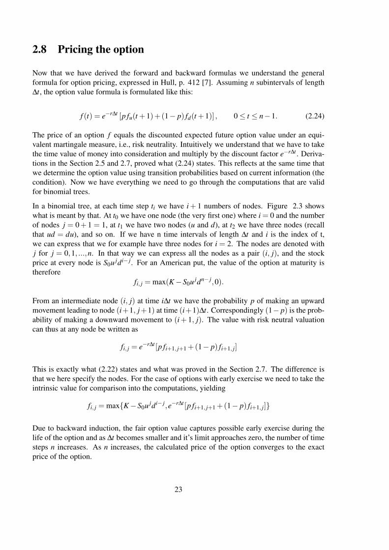
Now that we have derived the forward and backward formulas we understand the generalformula for option pricing, expressed in Hull, p. 412 [7]. Assuming n subintervals of length∆t, the option value formula is formulated like this:

f (t) = e−r∆t [p fu(t +1)+(1− p) fd(t +1)] , 0≤ t ≤ n−1. (2.24)

The price of an option f equals the discounted expected future option value under an equi-valent martingale measure, i.e., risk neutrality. Intuitively we understand that we have to takethe time value of money into consideration and multiply by the discount factor e−r∆t . Deriva-tions in the Section 2.5 and 2.7, proved what (2.24) states. This reflects at the same time thatwe determine the option value using transition probabilities based on current information (thecondition). Now we have everything we need to go through the computations that are validfor binomial trees.

In a binomial tree, at each time step ti we have i+ 1 numbers of nodes. Figure 2.3 showswhat is meant by that. At t0 we have one node (the very first one) where i = 0 and the numberof nodes j = 0+ 1 = 1, at t1 we have two nodes (u and d), at t2 we have three nodes (recallthat ud = du), and so on. If we have n time intervals of length ∆t and i is the index of t,we can express that we for example have three nodes for i = 2. The nodes are denoted withj for j = 0,1, ...,n. In that way we can express all the nodes as a pair (i, j), and the stockprice at every node is S0u jdi− j. For an American put, the value of the option at maturity istherefore

fi, j = max(K−S0u jdn− j,0).

From an intermediate node (i, j) at time i∆t we have the probability p of making an upwardmovement leading to node (i+1, j+1) at time (i+1)∆t. Correspondingly (1− p) is the prob-ability of making a downward movement to (i+ 1, j). The value with risk neutral valuationcan thus at any node be written as

fi, j = e−r∆t [p fi+1, j+1 +(1− p) fi+1, j]

This is exactly what (2.22) states and what was proved in the Section 2.7. The difference isthat we here specify the nodes. For the case of options with early exercise we need to take theintrinsic value for comparison into the computations, yielding

fi, j = max{K−S0u jdi− j,e−r∆t [p fi+1, j+1 +(1− p) fi+1, j]}

Due to backward induction, the fair option value captures possible early exercise during thelife of the option and as ∆t becomes smaller and it’s limit approaches zero, the number of timesteps n increases. As n increases, the calculated price of the option converges to the exactprice of the option.

23

(0,0)

(1,1)

(1,0)

(2,2)

(2,1)

(2,0)

(3,3)

(3,2)

(3,1)

(3,0)

t0 t1 t2 t3

Figure 2.3: Picture of notation in a binomial tree

2.9 Examples

Long European Call We can calculate how a European option should be priced at t0 in thefollowing way (example from Hull, page 243 [7]).

Let’s consider an asset with initial price S0 = 20. The strike price K = 21 and the time tomaturity is six months. The price of the underlying security will either go up or down by 10%.One time step equals three months, thus we have a two-step tree which is depicted4 in Figure2.4.

The pay-off from the call option at maturity is either 3.2 (node D), or zero (nodes E and F).This is calculated applying the formula shown earlier, pay-off long call = max{(St −K,0)},which gives 24.2−21 = 3.2. At nodes E and F the strike price exceeds the spot price, makingthe call worthless.

Now we work backwards through the tree to get the (hypothetical) price for the option at t1,i.e., nodes B and C. For that we have to take new parameters into consideration. At first we willcalculate the probabilities for up and down movements using (2.7). Let’s say that the risk freeinterest rate r = 0.12. We already know that ∆t = 0.25, u = 1.1 and d = 0.9. Therefore

p =e0.12×0.25−0.9

1.1−0.9= 0.6523

4In the second rows we show the asset prices and in the third rows the payoffs.

24

A20

1.2823

B22

2.0257

C180

D24.23.2

E19.8

0

F16.2

0

Figure 2.4: Model for European Call example

and(1− p) = 1−0.6523 = 0.3477

Now we can calculate the expected pay-off at node B by discounting the expected pay-off atthis point. We calculate the call at node B applying

e−r∆t(p fuu +(1− p) fud)

yielding

e−0.12×0.25(0.6523×3.2+0.3477×0) = 2.0257

Likewise we will obtain the result for the option value at t0:

e−0.12×0.25(0.6523×2.0257+0.3477×0) = 1.2823

An easier and faster way to calculate the price of the option is to use the formula

f = e−2r∆t [p2 fuu +2p(1− p) fud +(1− p)2 fdd] (2.25)

which is simply the squared version of (2.24).

Plugging in our variables yields

25

f = e−2×0.12×0.25 [0.65232(3.2)+2(0.6523)(0.3477)(0)+(0.3477)(2)(0)]= 1.2823

This is the exact same answer that we obtained using the tree-model for American options.The point of these extra calculations is to show that the value of an option always is the resultof iteratively working backwards. Since European options only can be exercised at maturityand not earlier, it is not necessary to do all those intermediate steps and the value of 1.2823should be computed much faster by (2.25).

Long American Put To show how the value of an American put is computed, we use thefollowing parameters from Hull, page 247 [7], which is shown in5 Figure 2.5.

S0 = 50, K = 52, r = 0.05, u = 1.2, d = 0.8, ∆t = 1 and T = 2 years

The probability of an upward movement equals

p =e0.05×1−0.8

1.2−0.8= 0.6282

Thus the probability of a downward movement is

(1− p) = 0.3718

The corresponding tree shows the price of the underlying asset at each node and the value ofthe option at maturity. Recall that the pay-off for put options equals max{(K−St),0}.

We can see that holding the option to maturity could give a pay-off of either 0, 4 or 20. Asin the previous example we can not know how the underlying asset is priced at maturity, butwe know that we have the possibility to exercise the option early. Thus we work backwardsthrough the tree to evaluate the option price at each time step. Then we compare the binomialvalue with the exercise value. The one that is greater tells how to proceed with the option. Ifthe binomial value is greater, we continue to hold the option. At t1 the option is either out ofthe money (node B), or it generates a pay-off of 12. We should clearly not exercise if we endup at B. Since the chance of a positive pay-off due to the end of the option is only 37.18%, thevalue of the put is expected to be low. Calculation yields

e−0.05×1(0.6282×0+0.3718×4) = 1.4147

The binomial value of 1.4147 is greater than the exercise value of zero. The option shouldtherefore be held.

5In the second rows we show the asset prices and in the third rows the payoffs.

26

A50

5.0894

B60

1.4147

C4012

D720

E484

F3220

Figure 2.5: Model for American Put example

If we ended up at node C, exercising would pay 12, holding the put could increase or decreasepay-off until maturity. The computation of the binomial price gives a value of 9.3646 (forsimplicity we skip the actual calculation). This is lower than the exercise price, thus exercisingat t1 is recommended and the value of the option is 12.

Conducting the corresponding computations for node A, we obtain the binomial price of5.0894 which is compared to early exercise value 2. The binomial price is greater, thus itshould not be exercised.

27

Chapter 3

Convergence of binomial model toGeometric Brownian motion

3.1 Introduction and Background

As we saw in the previous section, in Cox, Ross and Rubinstein’s approach, if n→ ∞, thebehavior of he binomial models can be approximated as a stochastic process in continuoustime. Black and Scholes 1973 [1] and Merton 1973 [15] assumed that the dynamic of a riskysecurity price follows a Geometric Brownian Motion. Following the Cox, Ross and Rubin-stein’s approach it is possible to see that the sequence of the binomial models also convergesto a Geometric Brownian Motion [12],[14]. To begin with, we can express some definitions:

Definition 3.1.1. A stochastic process (Wiener Process) W (t), 0≤ t ≤ T , is called a standardBrownian Motion if [12],[6],[14]1. W (0) = 0.2. W (t) is continuous on [0,T ] with probability 1.3. W (t) has independent increments.4. the increment W (t)−W (s) is normally distributed with mean zero and variance t− s.

Theorem 3.1.1. Let W (t)−W (s) be a normal random variable. A Brownian Motion with driftcoefficient {µ,µ ∈ R} and σ > 0 coefficients is

G(t) = µt +σW (t)

Here µ and σ2 may be time-dependent. [12],[6],[14].

Definition 3.1.2. Let G(t) be a Brownian motion with drift coefficient µ and diffusion coeffi-cient σ and S(0) be a positive real number. Then the process

S(t) = S(0)eG(t) = S(0)eµt+σW (t) (3.1)

28

is called Geometric Brownian Motion [12],[6],[14].

From now on we denote X = ST/S0 and Y = ln(ST/S0). Moreover, Y is a random variablewhich is normally distributed, and X is a random variable which is log-normally distributed.Now we will continue with some investigations on different results for the binomial models.Recalling (2.18) and (2.19) for the random variable X in a one-step binomial tree, we willhave1:

E[X ] = E[ST/S0] = p∗u+(1− p∗)d

V [X ] =V [(ST/S0)] = p∗u2 +(1− p∗)d2− (E[X ])2

Substituting the value of (E[X ])2 and simplifying V [X ] will yield:

V [X ] = p∗u2 +(1− p∗)d2− (p∗u+(1− p∗)d)2

= p∗u2 +d2− p∗d2− p∗2u2−2p∗(1− p∗)ud− (1− p∗)2d2

= p∗u2− p∗2u2 + p∗d2− p∗2d2−2p∗ud +2p∗2ud

= p∗(1− p∗)(u−d)2

To find the expected value and variance of the random variable Y we will do the followingsteps. Firstly, we know that the possible stock prices at a one step binomial tree are:

ST =

{S0u ,if stock goes up with probability pS0d ,if stock goes down with probability 1-p

Since S0 is constant we can divide both hand sides with S0. Additionally, for obtaining randomvariable Y we then can take the natural logarithm from both hand sides. Doing this will giveus:

Y = ln(

ST

S0

)=

{lnu ,if stock goes up with probability plnd ,if stock goes down with probability 1-p

Finally, considering Definition 2.2.3 and calculating the expected value with (2.5) will giveus:

E[Y ] = E [ln(ST/S0)] = p∗ lnu+(1− p∗) lnd

Considering Theorem 2.2.2 and calculating the variance with (2.6) will yield:

V [Y ] =V [ln(ST/S0)] = p∗[lnu]2 +(1− p∗)[lnd]2− (E[Y ])2

1A variable has log-normal distribution if the natural logarithm of the variable is normally distributed [7].

29

Substituting the value of (E[Y ])2 and simplifying V [Y ] will yield:

V [Y ] = p∗[lnu]2 +(1− p∗)[lnd]2− [p∗ lnu+(1− p∗) lnd]2

= p∗(lnu)2 +(lnd)2− p∗(lnd)2− p∗2 (lnu)2−2p∗(1− p∗) lnu lnd− (1− p∗)2 (lnd)2

= p∗(lnu)2− p∗2(lnu)2 + p∗(lnd)2− p∗2(lnd)2−2p∗ lnu lnd +2p∗2 lnu lnd

= p∗(1− p∗)[(lnu)2−2lnu lnd +(lnu)2]

= p∗(1− p∗) [lnu− lnd]2

Remark 3.1.1. Now we have a system of equations for both normal and log-normal randomvariables whit some unknown parameters p, u and d in a binomial lattice. We can rememberthat Cox, Ross and Rubinstein also ended up with two equations for expected value and vari-ance and three unknowns p, u and d. They solved this system of equations after calculating pand they let ud = 1 to obtain an equal number of equations and unknowns.

Now let us consider the sequence of binomial models and its convergence to the GeometricBrownian Motion.

3.2 The sequence of the binomial models and its conver-gence to Geometric Brownian Motion

In this part we will investigate the sequence of the binomial models and its convergence toGeometric Brownian Motion. To begin with, we can expand the sequence of the randomvariable Y as follows [12],[14]:

E[Y ] = E

[t

∑k=1

Yn,k

]= E

[ln

Sn,t

Sn,0

]= E [Yn,1 +Yn,2 + ...+Yn,t ] , 1≤ t ≤ n (3.2)

We have already calculated the expected value for Y , so the expected value at each time willbe:

E [Yn,t ] = p lnun +(1− p) lndn

We have already seen in the CRR model that as n→ ∞ the expected value and variance of ourprocess µT and σ2T [4].Moreover, we want the binomial model to converge to the Geometric Brownian Motion. Sowe will have:

Y = µt +σW (t) 0≤ t ≤ T

E[Y ] = µT V [Y ] = σ2T

Additionally, we know that in an n step binomial tree we have one random variable; let us callit m, which can take a certain number of upward movements. Then the number of downwardmovements will be n−m [4]. So the possible value for upward movements is un = um and

30

the possible value for downward movements is dn = dn−m. For simplicity we will denotexn = lnun and yn = lndn. Using the formulas for variance and expected value in the binomialmodel we will have [4],[12],[14]

E[Y ] = n [pxn +(1− p)yn] = µT

V [Y ] = np(1− p)(xn− yn)2 = σ

2T

considering the fact that dn < un, we know that yn < xn. We can re-write the equation asfollows and solve the system of two equations with two unknowns.

pxn +(1− p)yn = µT/n

xn− yn = σ

√T

np(1−p)

Solving this system of equations will give:xn =

µTn +σ

√1−p

p

√Tn

yn =µTn −σ

√p

1−p

√Tn

(3.3)

Recall (3.2). Since our sequence is a sequence of independent identically random variables,we will have nE[Yn,1] = µT and nV [Yn,1] = σ2T . Now we can apply the central limit theorem[12],[14]

limn→∞

P{Yn,1 +Yn,2 + ...+Yn,n−nE[Yn,1]√

nV [Yn,1]≤ x}= p{ ln(ST/S0)−µT

σ√

T≤ x}= Φ(x)

This proves that binomial models at time T , follow the normal distribution with mean µT andσ2T .

3.3 The sequence of binomial models and its convergence toBlack-Scholes model under risk-neutral probability

We have already shown that binomial models at time T converge to the normal distributionwith mean µT and variance σ2T . Moreover, recall that Black and Scholes 1973 and Merton1973 considered that the risky stock follows a Geometric Brownian Motion with drift coeffi-cient µ and diffusion coefficient σ . Black and Scholes proved that in their model, risky stocksare following the Geometric Brownian Motion with mean µ =

(r− σ2

2

)T and variance σ2T

[1]. We will follow Black and Scholes approach and we will derive their pricing formula in theappendix of this thesis. Since we are talking about pricing options via lattice approaches andour random variable ST is discrete, we would like to investigate if pricing options using the

31

binomial models converges to the Black-Scholes formula where ST is a continuous randomvariable. So we will investigate the convergence of the binomial model to the Black-Scholesmodel under risk neutral probability measure. First, for risk neutral probability measure wehave [12],[14]

p∗n =er T

n −dn

un−dn, 1− p∗n =

un− er Tn

un−dn(3.4)

From (3.3) we can obtain 2: xn = lnun⇒ un = exn = exp{

µTn +σ

√1−p

p

√Tn

}yn = lndn⇒ dn = eyn = exp

{µTn −σ

√p

1−p

√Tn

} (3.5)

Substituting (3.5) in (3.4), we will obtain:

p∗n =er T

n −du−d

=exp{

rTn

}− exp

{µTn −σ

√p

1−p

√Tn

}exp{

µTn +σ

√1−p

p

√Tn

}− exp

{µTn −σ

√p

1−p

√Tn

}=

exp{(r−µ)T

n

}− exp

{−σ

√p

1−p

√Tn

}exp{

σ

√1−p

p

√Tn

}− exp

{−σ

√p

1−p

√Tn

}

1− p∗n =u− er T

n

u−d=

exp{

µTn +σ

√1−p

p

√Tn

}− exp

{rTn

}exp{

µTn +σ

√1−p

p

√Tn

}− exp

{µTn −σ

√p

1−p

√Tn

}=

exp{

σ

√1−p

p

√Tn

}− exp

{(r−µ)T

n

}exp{

σ

√1−p

p

√Tn

}− exp

{−σ

√p

1−p

√Tn

}

It can be shown that limn→∞ p∗n = p and limn→∞(1− p∗n) = 1− p [12],[14].

Using the last result we can calculate the variance of binomial model as n→∞ [12],[14]:

limn→∞

V ∗[Y ] = limn→∞

np∗(1− p∗)(un− lndn)2 = lim

n→∞np(1− p)(xn− yn)

2

2Rendleman and Bartter 1979 got the same result in [16].

32

Substituting xn and yn from (3.3) we will calculate [12],[14]:

limn→∞

V ∗[Y ] = limn→∞

np(1− p)

[(µTn

+σ

√1− p

p

√Tn

)−

(µTn−σ

√p

1− p

√Tn

)]2

= limn→∞

np(1− p)

[σ

√Tn

(√1− p

p+

√p

1− p

)]2

= limn→∞

np(1− p)σ2T

n

(1− p

p+2

√1− p

p×√

p1− p

+p

1− p

)

= limn→∞

p(1− p)σ2T((1− p)2 + p2

p(1− p)+2)

= p(1− p)σ2T(

1p(1− p)

−2p(1− p)p(1− p)

+2)= p(1− p)σ2T

(1

p(1− p)

)= σ

2T

Secondly, for the expected value we have:

limn→∞

E∗[Y ] = limn→∞

n[p∗xn +(1− p∗)yn]

= limn→∞

n

[ exp{(r−µ)T

n

}− exp

{−σ

√p

1−p

√Tn

}exp{

σ

√1−p

p

√Tn

}− exp

{−σ

√p

1−p

√Tn

}×(µT

n+σ

√1− p

p

√Tn

)

+

exp{

σ

√1−p

p

√Tn

}− exp

{(r−µ)T

n

}exp{

σ

√1−p

p

√Tn

}− exp

{−σ

√p

1−p

√Tn

}×(µT

n−σ

√p

1− p

√Tn

)]

=

(r− σ2

2

)T

To solve the last equation the Maclaurin expansion was used. Furthermore, applying thecentral limit theorem we will obtain:

limn→∞

P∗{Y −nµn]

σn√

n≤ x}= p∗

{ ln(ST/S0)− (r− σ2

2 )T

σ√

T≤ x}= Φ(x)

which means, under risk-neutral probability measure, our stochastic process (binomial mod-els) at time T converges to normal distribution with mean (r− σ2

2 )T and variance σ2T .

33

3.4 Mean and variance of a random variable which is log-normally distributed

As we have shown in the previous part, binomial models at time T converges to normal distri-bution. In lots of scientific fields as well as finance, it is common to calculate and derive theexpectation and variance formulas for a random variable which is log-normally distributed. Sowe will try to show how the expected value and variance of a random variable can be derivedfrom a normal distribution. To begin with we write some definitions [21].

Definition 3.4.1. A random variable U is said to have a normal probability distribution if andonly if, for σ > 0 and −∞ < µ < ∞, the density function of U is:

f (u) =1

σ√

2πe−(u−µ)2/(2σ2), −∞ < u < ∞

and the following theorem tells us [21]:

Theorem 3.4.1. If U is a normally distributed random variable with parameter µ and σ , then:

E[U ] = µ and V [U ] = σ2

It is possible to transform a normal random variable U to a standard normal random variableZ by [21]:

Z =U−µ

σ

Applying Definition 3.4.1 and Theorem 3.4.1 to our random variable Y , we will have:

f (y) =1

σ√

2πe−(y−µy)

2/(2σ2y ), −∞ < y < ∞

where we have already calculated the mean and variance of binomial models at time T and itsconvergence to normal distribution:

E[Y ] = µy = µT and V [Y ] = σ2y = σ

2T

Now, we can continue with another definition [21]:

Definition 3.4.2. If a random variable Y is normally distributed with mean µy and varianceσ2

y and X = eY [equivalently, Y = lnX], then X is said to have a log-normal distribution.Then the density function for X is:

f (x) =

{ (1

xσ√

2π

)e−(lnx−µy)

2/(2σ2y ), x > 0

0, elsewhere.(3.6)

34

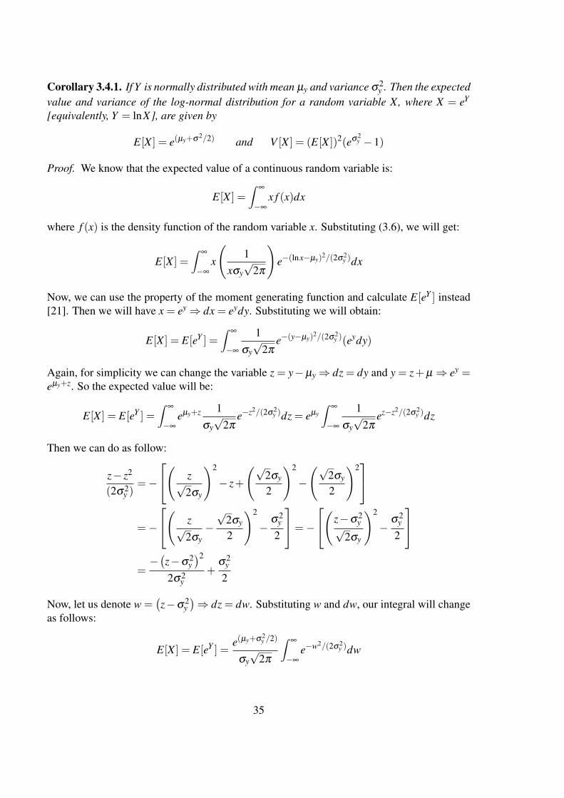
Corollary 3.4.1. If Y is normally distributed with mean µy and variance σ2y . Then the expected

value and variance of the log-normal distribution for a random variable X, where X = eY

[equivalently, Y = lnX], are given by

E[X ] = e(µy+σ2/2) and V [X ] = (E[X ])2(eσ2y −1)

Proof. We know that the expected value of a continuous random variable is:

E[X ] =∫

∞

−∞

x f (x)dx

where f (x) is the density function of the random variable x. Substituting (3.6), we will get:

E[X ] =∫

∞

−∞

x

(1

xσy√

2π

)e−(lnx−µy)

2/(2σ2y )dx

Now, we can use the property of the moment generating function and calculate E[eY ] instead[21]. Then we will have x = ey⇒ dx = eydy. Substituting we will obtain:

E[X ] = E[eY ] =∫

∞

−∞

1σy√

2πe−(y−µy)

2/(2σ2y )(eydy)

Again, for simplicity we can change the variable z = y−µy⇒ dz = dy and y = z+µ ⇒ ey =eµy+z. So the expected value will be:

E[X ] = E[eY ] =∫

∞

−∞

eµy+z 1σy√

2πe−z2/(2σ2

y )dz = eµy

∫∞

−∞

1σy√

2πez−z2/(2σ2

y )dz

Then we can do as follow:

z− z2

(2σ2y )

=−

( z√2σy

)2

− z+

(√2σy

2

)2

−

(√2σy

2

)2

=−

( z√2σy−√

2σy

2

)2

−σ2

y

2

=−

(z−σ2y√

2σy

)2

−σ2

y

2

=−(z−σ2

y)2

2σ2y

+σ2

y

2

Now, let us denote w =(z−σ2

y)⇒ dz = dw. Substituting w and dw, our integral will change

as follows:

E[X ] = E[eY ] =e(µy+σ2

y /2)

σy√

2π

∫∞

−∞

e−w2/(2σ2y )dw

35

Solving this integral is complicated, but we can use a typical trick and calculate the squarevalue of the expected value and then the positive square root of the result will be the answer.So, we will have:

(E[X ])2 = (E[eY ])2 =e(2µy+σ2

y )

2πσ2y

∫∞

−∞

∫∞

−∞

e−(v2+w2)/(2σ2

y )dvdw

To solve this integral we can use polar form and change variables v = r cosθ , w = r sinθ ,dvdw = det(J)drdθ and det(J) = r. Where det(J) is the Jacobian . So we will have:

v2 +w2 = r2 cos2θ + r2 sin2

θ = r2(cos2+sin2) = r2

and the integral will be:

(E[X ])2 = (E[eY ])2 =e(2µy+σ2

y )

2πσ2y

∫∞

0

∫ 2π

0re−r2/(2σ2

y )drdθ

=e(2µy+σ2

y )

σ2y

∫∞

0re−r2/(2σ2

y )dr

=−e(2µy+σ2y )∫

∞

0

−2r2σ2

ye−r2/(2σ2

y )dr

=−e(2µy+σ2y )[e−r2/(2σ2

y )]∞

0

=−e(2µy+σ2y )( lim

r→∞e−r2/(2σ2

y )− e0)

=−e(2µy+σ2y )(0−1) = e(2µy+σ2

y )

taking square root of the last result, will yield:

E[X ] = E[eY ] =[e(2µy+σ2

y )]1/2

= e(µy+σ2y /2)

Substituting the value for σ2y = σ2T and µy = µT , we will obtain the mean of the log-normal

distribution.

E[X ] = e(µ+12 σ2)T

To calculate the variance we have:

V [X ] = E[(X)2]− (E[X ])2 (3.7)

We have already known the result of (E[X ])2. To calculate the E[X2] we can use the propertyof the moment generating function [21] and we will have:

E[X2] = E[e2Y ] =∫

∞

−∞

1σy√

2πe−(y−µy)

2/(2σ2y )(e2ydy)

36

Again, for simplicity we can change the variable u = y−µy⇒ du = dy and y = u+µ⇒ e2y =

e2(µy+z). So, the expected value will be:

E[X2] = E[e2Y ] =∫

∞

−∞

e2(µy+u) 1σy√

2πe−u2/(2σ2

y )du

= e2µy

∫∞

−∞

1σy√

2πe2u−u2/(2σ2

y )du

= e2µy

∫∞

−∞

1σy√

2πe−(u2−4uσ2

y )

2σ2y du

= e2µy

∫∞

−∞

1σy√

2πe−(u2−4uσ2

y +(2σ2y )

2−(2σ2y )

2

2σ2y du

= e2(µy+σ2y )∫

∞

−∞

1σy√

2πe−(u−2σ2

y )2

2σ2y du

= e2(µy+σ2y )

Substituting the value for E[X2] = e2(µy+σ2y ) in (3.7), we will get:

V [X ] = e2(µy+σ2y )− e(2µy+σ2

y ) = e2µy+σ2y

(eσ2

y −1)

And finally, substituting σ2y = σ2T and µy = µT , we will get:

V [X ] = e(2µ+σ2)T(

eσ2T −1)

Remark 3.4.1. Calculating such integrals is usual for continuous random variables. So, hav-ing proper skills to calculate ordinary and stochastic integrals is vital for a financial analyzer.

Remark 3.4.2. Often in literature we can see that the authors do not calculate the integ-rals; they jumped to the results. Considering the calculation above we can explain it. Aswe saw a density function for a normal random variable X ∼ N[µ,σ ] is given by φ(x) =

1σ√

2πe−(x−µ)2/2σ2

, then considering the calculations above, we know that the distribution

function of a normal random variable has the value of Φ(X) =∫ X−∞

φ(x)dx. As an example,for a standard normal random variable Z, where µ = 0 and variance is σ = 1 or equival-ently Z ∼ N[0,1], we can directly say that the density function of a standard normal randomvariable Z is φ(z) = 1√

2πe−z2/2 and Φ(Z) =

∫ Z−∞

φ(z)dz. So, if we can make the form of ourintegral like an integral of a density function for the standard normal random variable, thenwe can find the probability (area under normal curve) from the standard normal probabilitytable. Additionally, if we have a normal random variable instead of standard normal variable,we can transform the normal variable to standard normal random variable and again use thetable to find the probability. Finally, it is easy to say the area under the any density function isone or equivalently

∫∞

−∞φ(z)dz = 1 [21].

37

Chapter 4

Different approaches on BinomialModels

In the previous chapter we calculated the expected value and variance of the normal and log-normal distribution for normal and log-normal random variables. Then we calculated the ex-pected value and variance of the binomial models which converges to a Geometric BrownianMotion. Moreover, we have seen that the sequence of binomial models at time T convergesto the Geometric Brownian Motion under risk-neutral probability. So if we want to estim-ate binomial models with Log-normal distribution and at the same time we want that ourmodel converges to a Geometric Brownian Motion, we can substitute the expected value1

µy =(

r− σ2

2

)T and variance σ2

y = σ2T of the Geometric Brownian Motion to our expectedvalue and variance formulas which we have obtained for log-normal distribution [17]. Thuswe will have:

limn→∞

E∗[X ] = limn→∞

n[pu+(1− p)d]

= e(µy+12 σ2

y ) = e(r−12 σ2+ 1

2 σ2)T = erT

limn→∞

V ∗[X ] = limn→∞

np(1− p)(u−d)2

= e(2µy+σ2y )(

eσ2y −1

)= e(2r−σ2+σ2)T

(eσ2T −1

)limn→∞

V ∗[X ] = e2rT(

eσ2T −1)

X ∼ LN[rT,σ2T

]Again, we will have two equations for expected value and variance and three unknowns u, dand p. We can choose different value for either p, u or d to obtain our third equation and makea survey of different binomial models where we want results to converge to the Geometric

1We know that in risk neutral probability measure, or equivalent Martingale probability measure, the driftcoefficient is equal to the risk-free interest rate.

38

Brownian Motion [17]. Additionally, our calculation was for n step binomial models. Con-sidering this fact, we can say that in each step we will have ∆t = T/n, and we can calculatethe expected value and variance for each step in the binomial tree. So for X = Si+1

Siwhich is

log-normally distributed we will have [17]:

X =Si+1

Si

E[X ] = pu+(1− p)d = er∆t

V [X ] = p(1− p)(u−d)2 = e2r∆t(

eσ2∆t−1)

X ∼ LN[r∆t,σ2

∆t]

For Y = ln(

Si+1Si

)which is normally distributed, we will have:

Y = ln(

Si+1

Si

)E[Y ] = p lnu+(1− p) lnd = (r− σ2

2)∆t

V [Y ] = p(1− p) [lnu− lnd]2 = σ2∆t

Y ∼ N[(

(r− σ2

2

)∆t,σ2

∆t]

Now we have the system of two equations for both normal and log-normal random variableswhit three unknown parameters p, u and d in a binomial lattice. IN next two sections we willintroduce the third equation when the stock price is normally and log-normally distributed byp = 1/2 and ud = 1 and we will try to calculate p, u and d. Then we will make a survey onsome well-known and famous binomial models2[17].

4.1 Random variable Y = ln(

Si+1Si

)is normally distributed

When the random variable Y = ln(

Si+1Si

)is normally distributed, we will have two equations

for expected value and variance and three unknowns p, u and d. Here we will introduce oneextra equation to increase our equations to three and then we will solve a system of threeequations and three unknowns.

2We had already written a preliminary version of our thesis when we found an interesting paper "Two-StateOption Pricing: Binomial Models Revisited" by Jabbour, Kramin and Young [8]. We would suggest that thereader looks at that paper as well.

39

4.1.1 Introducing the third equation by p = 1/2

Writing the equations for the expected value and variance of the random variable Y , which isnormally distributed, we will have two equations and three unknowns:

E[Y ] = p lnu+(1− p) lnd = (r− σ2

2)∆t

V [Y ] = p(1− p) [lnu− lnd]2 = σ2∆t

Substituting p = 1/2 we will get the system of two equations with two unknowns.{(lnu− lnd)2 = 4σ2∆tlnu+ lnd = (2r−σ2)∆t

We denote x = lnu and y = lnd. Moreover, since u > d⇒ x > y, we will have:{x− y = 2σ

√∆t

x+ y = (2r−σ2)∆t

we will obtain:

x = (r− σ2

2)∆t +σ

√∆t⇒ u = e(r−

σ22 )∆t+σ

√∆t

y = (r− σ2

2)∆t−σ

√∆t⇒ d = e(r−

σ22 )∆t−σ

√∆t

Remark 4.1.1. The value for p is different in the Jarrow-Rudd model, but as we will see later,the values for the u and d factors in our approach are exactly the same as the values for uand d factors which have been derived by Jarrow and Rudd. However, Jarrow and Rudd haveshown that p = 1/2 as ∆t→ 0 [10],[9].Remark 4.1.2. We can consider the formula which was obtained by Rendleman and Bartter[16], which is as follows u = exp

{µTn +σ

√1−p

p

√Tn

}d = exp

{µTn −σ

√p

1−p

√Tn

}Where p is unknown. Susbtituting p = 1/2 we will obtain exactly the same result for u and din our calculations.Remark 4.1.3. In this model ud = e(2r−σ2)∆t , whereas in the CRR model ud = 1.

4.1.2 Introducing the third equation by ud = 1

Again, we have two equations and three unknowns.

E[Y ] = p lnu+(1− p) lnd = (r− σ2

2)∆t

V [Y ] = p(1− p) [lnu− lnd]2 = σ2∆t

40

Substituting d = 1/u we will get a system of two equations with two unknowns.{p(1− p)(lnu− lnu−1)2 = p(1− p)(lnu+ lnu)2 = σ2∆tp lnu+(1− p) lnu−1 = p lnu− (1− p) lnu = (r− σ2

2 )∆t

We denote x = lnu and y = lnd. Moreover, since u > d⇒ x > y, we will have:{4p(1− p)x2 = σ2∆tpx− (1− p)x = x[p− (1− p)] = (r− σ2

2 )∆t

we will obtain:

x =(r− σ2

2 )∆t2p−1

p− p2 =σ2∆t4x2

Substituting and denoting a = (r− σ2

2 )2∆t we can solve the equations above for p:

p2− p+σ2∆t

4(

(r−σ22 )∆t

2p−1

)2 = 0

p2− p+σ2(4p2−4p+1)

4(r− σ2

2 )2∆t= 0⇒ ap2−ap+σ

2 p2−σ2 p+

σ2

4= 0

p2(a+σ2)− p(a+σ

2)+σ2 = 0

p2− p+σ2

4(a+σ2)= 0

then

p1,2 =1±√(−1)2−4σ2/4(a+σ2)

2

p =12± 1

2×

√a+σ2−σ2

a+σ2 =12+

12×

√a√

a+σ2

p1,2 =12± 1

2×

√∆t(r− σ2

2 )√

∆t√

σ2

∆t +(r− σ2

2 )2

p=12+

12×

(r− σ2

2 )√σ2

∆t +(r− σ2

2 )2

41

To calculate x we can use the variance formula which is much more convenient and will helpus to avoid the quadratic calculation.

V [Y ] = p[ln(u)]2 +(1− p)[ln(d)]2− (E[Y ])2 = σ2∆t

p[ln(u)]2 +(1− p)[ln(d)]2−[(r− σ2

2)∆t]2

= σ2∆t

p[ln(u)]2 +(1− p)[ln(u−1)]2−[(r− σ2

2)∆t]2

= σ2∆t

p[ln(u)]2 +(1− p)[−ln(u)]2−[(r− σ2

2)∆t]2

= σ2∆t

px2 +(1− p)(−x)2−[(r− σ2

2)∆t]2

= σ2∆t

x =

√σ2∆t +

[(r− σ2

2)∆t]2

u = e

√σ2∆t+

[(r−σ2

2 )∆t]2

d = e−√

σ2∆t+[(r−σ2

2 )∆t]2

Remark 4.1.4. Our calculation to derive p raise a controversial question. Can we obtaintwo answers for p which both lie between zero and one? Perhaps yes. Because, the term12 ×

(r−σ22 )√

σ2∆t +(r−σ2

2 )2must lie between −1/2 and 1/2, since, the probability p must lie between

zero and one. So perhaps we can say:

p1,2 =12 ±

12 ×

(r−σ22 )√

σ2∆t +(r−σ2

2 )2

So, if we choose a negative sign, then p can be close to zero and if we choose a plus sign, pcan be close to one, which is what we expected.

Remark 4.1.5. In this model we have the same arguments as in all binomial models which wehave considered. If n→ ∞ then ∆t→ 0 then limn→∞ pn = 1/2.

42

4.2 Random variable X =Si+1

Siis log-normally distributed

When the random variable X = Si+1Si

is log-normally distributed, we will have two equations forexpected value and variance and three unknowns p, u and d. Here we will introduce one extraequation to increase our equations to three and then we will solve a system of three equationsand three unknowns.

4.2.1 Introducing the third equation by p = 1/2

Writing a system of two equations and three unknowns, we will have:

E[X ] = pu+(1− p)d = er∆t

V [X ] = p(1− p)(u−d)2 = e2r∆t(

eσ2∆t−1)

Substituting p = 1/2 we will obtain:

u+d = 2er∆t ⇒ u = 2er∆t−d

(u−d)2 = 4e2r∆t(

eσ2∆t−1)

substituting u:

(2er∆t−d−d)2 = (2er∆t−2d)2

= (4e2r∆t−8der∆t +4d2) = 4e2r∆t(

eσ2∆t−1)

⇒d2−2er∆td− e2r∆t(

eσ2∆t−2)= 0

d1,2 =2er∆t±

√(−2er∆t)2 +4e2r∆t

(eσ2∆t−2

)2

d1,2 = er∆t±√

e2r∆t + e2r∆t(eσ2∆t−2

)d1,2 = er∆t± er∆t

√eσ2∆t−1

since d < u then:

u = er∆t(

1+√

eσ2∆t−1)

d = er∆t(

1−√

eσ2∆t−1)

43

Remark 4.2.1. In this model, we will have:

ud = e2r∆t(

12−[√

eσ2∆t−1]2)= e2r∆t

(2− eσ2∆t

)

4.2.2 Introducing the third equation by ud = 1

Solving the following equation for p we will have:

E[X ] = pu+(1− p)d = er∆t

⇒ pu+d− pd = p(u−d)+d = er∆t

⇒ p =er∆t−du−d

=uer∆t−1

u2−1

and solving the variance equation for u we will get:

V [X ] = p(1− p)(u−d)2 = e2r∆t(

eσ2∆t−1)

⇒ uer∆t−1u2−1

× u(u− er∆t)

u2−1×(

u2−1u

)2

= e2r∆t(

eσ2∆t−1)

⇒ u2er∆t−ue2r∆t−u+ er∆t

u= e2r∆t

(eσ2∆t−1

)⇒ u2er∆t−ue2r∆t−u+ er∆t−ue2r∆t

(eσ2∆t−1

)= 0

⇒ u2(

er∆t)−u(

e(2r+σ22 )∆t +1

)+ er∆t = 0

⇒ u1,2 =

(e(2r+σ2

2 )∆t +1)±√(

e(2r+σ22 )∆t +1

)2−4e2r∆t

2er∆t

u =12

e−r∆t[e(2r+σ2)∆t +1

]+

√14

e−2r∆t[e(2r+σ2)∆t +1

]2−1

d =12

e−r∆t[e(2r+σ2)∆t +1

]−√

14

e−2r∆t[e(2r+σ2)∆t +1

]2−1

Remark 4.2.2. As we can see in this model, the value of p is equal to the risk-neutral prob-ability measure in the CRR model, but the u and d factors are different. The reason is, in ourequation for variance we have a different value compared to the CRR model because from thebeginning, we constructed our model in such a way that our binomial model converges to theGeometric Brownian Motion.

44

4.3 The Jarrow-Rudd model

This model was proposed by Jarrow and Rudd [10]. However, we used additional literatureto study this model [9],[17]. We have already calculated the expected value and varianceof a random variable which is log-normally distributed. Using the previous result we have[9]:

E[X ] = E[

ST

S0

]= exp

{µT +

σ2

2T}

Since S0 is constant, the equation above can be rewritten as:

E[ST ] = S0 exp{

µT +σ2

2T}

Moreover, we know that the option pricing follows a martingale process. Thus under theequivalent martingale probability measure we have [9]:

E p∗[ST |S0] = S0 exp{

µ̂T +σ2

2T}

(4.1)

and considering the fact that in the risk-neutral world the expected return on a stock must beequal to the risk-free interest rate, we can write the next equation as follows [9]:

S0 = e−rT E p∗[ST |S0] (4.2)

Substituting (4.1) into (4.2) we will obtain µ̂ = r− σ2

2 , which means in the risk-neutral worldthat the drift coefficient must be equal to r− σ2

2 .Now we can approximate this process in the discrete binomial model. It follows [9]:

St+1 = St

{u = e(r−

σ22 )∆t+σ

√∆t with probability p∗

d = e(r−σ22 )∆t−σ

√∆t with probability 1− p∗

where p∗ = erT−du−d , and Y = St+1

St∼ N

[((r− σ2

2

)∆t,σ2∆t

]. If we substitute the value of u and

d in our probability equation we will obtain [9]:

p∗ =e

σ22 ∆t− e−σ

√∆t

eσ√

∆t− e−σ√

∆t

Moreover, if we calculate the limit, we will obtain [9]:

lim∆t→0

p∗ = lim∆t→0

eσ22 ∆t− e−σ

√∆t

eσ√

∆t− e−σ√

∆t=

12

Remark 4.3.1. As we can see, Jarrow and Rudd used a significantly different approach fromBlack and Scholes. However, they find the same result for the drift and diffusion coefficientunder risk-neutral probability measure.

Remark 4.3.2. In the Jarrow-Rudd model ud = e(2r−σ2)∆t , whereas in the CRR model ud = 1.

45

4.4 The Tian model

Tian introduce his binomial model in discrete time with following p, u and d factors:

p =M−du−d

, q = 1− p =u−Mu−d

u =MV

2

[V +1+

√V 2 +2V +3

]d =

MV2

[V +1−

√V 2 +2V +3

]

Now, let’s see how he derived equations above and what M and V stand for.

Tian constructed his model assuming that in a risk neutral world, the stock price is followinga stochastic process which is given by following the stochastic differential equation [19]:

dS(t)S(t)

= rdt +σdW

Then he considered the logarithmic transformation of the process above. To do so, we de-note F = ln(S(t)) and then we will apply Itô’s formula to the SDE above, so we will have[19]:

dF =∂F∂ t

dt +∂F∂S

dS+12

∂ 2F∂S2 (dS)2

dF = 0+1S

dS− 12S2 (dS)2

dF =1S(rSdt +σSdW )− 1

2S2

(σ

2S2(dW )2)dF = (rdt +σdW )− 1

2σ

2dt

dF =

(r− σ2

2

)dt +σdW

d lnS(t) =(

r− σ2

2

)dt +σdW (4.3)

Notice that (dW )2 = dt and (dt)2 = dtdW = 0. Considering (4.3) and the discussion wehad before, it is obvious that in (4.3) the one dimensional distribution is following a normaldistribution with mean (r− σ2

2 )t and variance σ2t. Thus the mth non-central moment of thestock price can be interpreted by [19]:

E[S(t)m|S0] = Sm0 exp

{(mr+(m−1)

σ2

2

)t}

46

This is a formula for a stochastic process in continuous time. To approximate this formula indiscrete time with an n-step binomial model, we can say that ∆t = T

n . We assumed that theprice of a stock follows a binomial process which sometimes is called a two-jump process3.Now, as we have discussed before, we want our binomial model to converge to the log-normaldistribution in continuous time. So, we have to choose the parameters u, d, p and q in a waythat guarantees our objective. Using our knowledge and the proofs we did before, we knowthat in the binomial models, our random variable Y , is normally distributed. Moreover, us-ing the result for the transformation of random variable X which is log-normally distributed,we can express the expected value and variance of binomial models at time T when our ran-dom variable is log-normally distributed. Thus we can write the following three equations[19]:

p+q = 1

pu+qd = er∆t = M

pu2 +qd2 = e(2r+σ2)∆t = M2V

Tian denotes M = er∆t and V = eσ2∆t . Substituting q = 1− p we have two equations and threeunknowns. Cox, Ross and Rubinstein considered a recombining tree with u = 1/d, but Tianconsidered that the third moments of the discrete time process is also correct according to acontinuous time process, so he obtained the forth equation [19]:

pu3 +(1− p)d3 = M3V 3

Solving this system of equations, Tian got [19]:

p =M−du−d

, q = 1− p =u−Mu−d

u =MV

2

[V +1+

√V 2 +2V +3

]d =

MV2

[V +1−

√V 2 +2V +3

]

Remark 4.4.1. By comparing and contrasting the CCR model and the Tian model, we can saythat in the CRR model the variance is correct in the limit case and when ∆t → 0, whereas inthe Tian model, both mean and variance are true for any given ∆t [19].

Remark 4.4.2. Tian chose the correct third moment, but CCR chose ud = 1 for simplicity. Inthe Tian model we have ud = (MV )2 [19].

3See [19]

47

4.5 The Trigeorgis model

Trigeorgis began with the design of the log-transformed binomial model. Again, he consideredthe diffusion process as follows [20]:

dS(t)S(t)

= αdt +σdW

where α is expected value, σ is standard deviation and W is a Wiener process. Moreover,X(t)≡ lnS(t) follows Brownian motion. So under risk-neutral probability we will have α = rand our process when, S(t) is log-normally distributed, will be [20]:

dX = ln(

S(t +dt)S(t)

)=

(r− σ2

2

)dt +σdW

Again, in this process, ln(

S(t+dt)S(t)

)or equivalently dX is normally distributed. So, we have

[20]:

E[dX ] =

(r− σ2

2

)dt, V [dX ] = σ

2dt

In order to approximate our continuous process in discrete time in each sub-interval ∆t = T/n,X will follow a Markov random walk which with risk-neutral probability p goes up by theamount ∆X = H ≡ u and with risk-neutral probability 1− p goes down by the amount of∆X =−H ≡ d [20]. It is easy to see that this binomial model is recombining. Thus calculatingthe expected value and variance for this Markov process we will obtain [20]

E[∆X ] = pH +(1− p)(−H) = 2pH−H ≡ pu+(1− p)d

V [∆X ] = p(1− p)(2H)2 = 4pH2−4p2H2 ≡ p(1− p)(u−d)

V [∆X ] = H2− (H2−4pH2 +4p2H2) = H2− (2pH−H)2 = H2− (E[∆X ])2

We will obtain a system of two equations with two unknowns [20]:

2pH−H = 2p∆X−∆X = ∆X(2p−1) =(

r− σ2

2

)∆t

4pH2−4p2H2 = 4p(∆X)2(1− p) = σ2∆t

Solving the equations we will obtain [20]:

∆X =

√σ2∆t +

(r− σ2

2

)2

(∆t)2

p =12

[1+(

r− σ2

2

)∆t∆X

]Remark 4.5.1. It is easy to see that lim∆t→0 p = 1/2 in Trigeorgis model as well.

48

4.6 The Leisen-Reimer model

One of the latest binomial models was proposed by Leisen and Reimer in 1996 [13],[17]. Theyconsidered the Black-Scholes formula and the convergence of different binomial models to theBlack-Scholes formula. Leisen and Reimer proposed and proved a theorem about the order ofconvergence in different binomial models. They showed that the previous models in discretetime such as CCR, JR, Tian and more, have convergence to the Black and Scholes results withorder one. Their model however, has a second order of convergence (quadratic convergence)[13]. To begin with, we write the Black-Scholes formula 4:

c(t,S0) = S0N(d1)−Ke−r(T−t)N(d2), d1,2 =ln(S0/K)+(r± σ2

2 )(T − t)σ√

T − t

and the CRR option pricing formula5 [4]:

cn(tn0 = 0,S0) = S0Φ(a;n, p′n)−Kr−n

n Φ(a;n, pn)

where [13],[4]:

pn =rn−dn

un−dnp′n = pn

un

rna =

ln(K/S0)−n lndn

lnun− lndn

Then they consider the fact that in all approaches which they have followed in the binomialmodel, the probability p is approximated with the standard normal function N(z), where the allinput arguments are determined by some adjustment function z = h(a;n, p) [13]. Leisen andReimer denoted 6 a as the number of upward movements of the asset price to exceed strikeprice in a n step binomial tree (lattice) with martingale probability measure p [13] instead.Then they made an inverse transformation of the adjustment function where h(a;n, p) specifiesthe distribution parameter h−1(z) = p to approximate P = N(z) with P ≈ 1−Φ(a;n, p) [13].Then they used the Peizer and Pratt derivation of the inversion formula to the Camp-Paulsonmethod, one with7 [case : a+1/2 = n− (a+1/2),n = 2a+1] [13]:

h−1(z) =12∓

14− 1

4exp

{−

(z

n+ 13

)2(n+

16

)}1/2

After introducing the discussion above, Leisen and Reimer solved the system of equationsin such way which guarantees the convergence of the binomial model. In other words, theyneeded to derive un, dn and pn. After a little algebra they obtained their new binomial modelwith the following parameters [13]:

p′n = h−1(d1) pn = h−1(d2)

un = rnp′npn

dn =rn− pnun

1− pn

4To see the derivation of Black-Scholes option pricing formula, see Appendix A.5To see the derivation see [4].6This condition in the CRR model is given by a≡ smallest non-negative integer greater than ln(K/S0)−n lndn

lnun−lndn.

7Two see the result for Camp-Paulson inversion and Peizer-Pratt method two, see [13].

49

Remark 4.6.1. By having the parameter Z in the Leisen-Reimer model, we can get a uniquedistribution parameter p for each pair of (a,n). Thus in the continuous model the parametera(n) can be chosen freely, whereas in the discrete case a(n) and a′(n) can be chosen freely butthey must be equal to determine pn and p′(n) in the system of equations above [13].

Remark 4.6.2. With inverse transformation, we have to have an odd number of steps in thismodel [13].

50

Chapter 5

Trinomial Model

Except up and downward movements, we could consider no movement at all. We introducea new variable m to describe a stable middle path. A three-step tree is depicted in Figure5.1.

For a random walk with three possible directions our random variable X j with j ∈ Z+ behaveslike this:

P(X j = u) = pu = p1

P(X j = m) = 1− pu− pd = p2

P(X j = d) = pd = p3

where p1 + p2 < 1 and ∑ pi = 1 with i = 1,2,3.

If we have k + l + (n− k− l) = n trials, event u will occur k times, event d will occur ltimes and event m will occur (n− k− l) times, so the sequence of events gives an outcome ofukmn−k−ldl . This is easier to understand if we look at Figure 5.1. Following a path consistingof n = 3 steps, gives a sequence of, for instance, uud which is u2m0d1. In this example wereach node (3,4) which also can be reached in two more ways (udu and duu), three in total.Therefore, we say that the coefficient for a distribution with two up and one down movementis equal to three. Looking at node (3,3) you will see that there are six ways of combining oneof each movements, (umd,udm,mud,mdu,dmu and dum) in order to get to this node. Herethe coefficient is 6.

There are 3n different paths which in this particular three step case is 33 = 27. This is also the

sum of the coefficients. If p1 = p2 = p3, each of the paths would have probability13n , but in

cases where this is not true, the probability for each path depends on the respective values forp1, p2, p3. If we knew the probability for each event, we can calculate the probability of eachsequence of events. A particular path contains of a certain distribution of events, which meansthat the probability that event u occurs k times is pk

1. In general the probability for obtaining

51

one particular sequence ω isP(ω) = pk

1 pl2 pn−k−l

3

As mentioned we could have similar sequences with the same amount of ups and downs, butin different orders and the total number of these is(

nk

)(n− k

l

)=

n!k!l!(n− k− l)!

Thus the probability of one particular outcome, i.e., the trinomial probability distribution isthe joint probability function for X1,X2,X3

P(X1 = k,X2 = l,X3 = (n− k− l)) =(

nk

)(n− k

l

)pk

1 pl2 pn−k−l

3

5.1 Properties of the trinomial distribution

We can think of the trinomial distribution as the composition of events that fall into one cat-egory and all other events that fall into another category. For the case of evolution of assetprices we say that upward movements (event X) occur with probability p and middle- anddownward movement (event Y ) with probability q = 1− p. This makes it clear that we havemarginal distributions for the two categories with binomial marginal probability distributions.It follows that

E(X) = np, V (X) = npq

5.1.1 A stretch to the multinomial distribution

The same thinking as for trinomial distribution applies to multinomial distribution. The jointprobability function for X1,X2, ...Xk is given by

p(x1,x2, ...,xk) =n!

x1!x2!...xk!px1

1 px22 ...pxk

k

where

k

∑i=1

pi = 1,k

∑i=1

xi = n, pi ≥ 0, xi ≥ 0

The expected value and variance of the marginal distributions are

52

E(Xi) = npi, V (Xi) = npiqi

Trinomial and multinomial models are an extension of binomial models. There are moreparameters involved, but the approach is the same, hence the similarity in the formulas. Infact, the binomial model is a special case of multinomial models. The easiest way to seethat is to think about the marginal distribution. If we have two probabilities, we have twoscenarios with their corresponding events; if we have three probabilities, we have one scenariowith its corresponding event, and another scenario where this event not occurs. If we have nprobabilities, we can again say that we have two scenarios; one with its event and another onewhere the first one not occurs (but all the others). This is well explained in Wackerly, et al,pages 278 and 279 [21] which is the basic material used up to now in this section. There aremore explanations within the statements compared to the binomial model because it might bea little bit harder to cope with the formulas when a third variable is involved.

(0,0)S0

(1,2)S0u

(1,1)S0

(1,0)S0d

(2,4)S0u2

(2,3)S0u

(2,2)S0

(2,1)S0d

(2,0)S0d2

(3,6)S0u3

(3,5)S0u2

(3,4)S0u

(3,3)S0

(3,2)S0d

(3,1)S0d2

(3,0)S0d3

Figure 5.1: Three-step trinomial tree

5.2 Boyle’s approach of deriving probabilities

In his paper [2], Boyle derived the values for the three probabilities and the values for u andd implying that the log normal continuous distribution of the evolution of the stock price

53

has the same properties as the discrete distribution, i.e., mean and variance of the respectivedistributions equal each other. As we have seen before, the probabilities for the movementssum up to 1. Therefore it is valid to substitute p2 by 1− p1− p3. In the continuation of theexplanation of this approach we use the same notation as Boyle which is

Su, S and Sd = price of the underlying asset after an upward, downward or horizontal move-ment respectively,r = interest rate, continuously compounded,σ2 = variance of return,

h = length of one time interval, d =1u

.

The equation regarding equality between discrete and log normal continuous expected valueis

SM = Serh

SM = p1Su +(1− p1− p3)S+ p3Sd

We rewrite this and obtain

p1(u−1)+ p3

(1u−1)= M−1 (5.1)

The equation regarding equality between discrete and log normal continuous expected valueis

S2V = S2V = S2M2exp[(σ2h)−1)]

S2V = p1(S2u2−S2M2)+(1− p1− p3)(S2−S2M2)+ p3(S2

u2 −S2M2)

which in rewritten form gives

p1(u2−1)+ p3

(1u2 −1

)=V +M2−1. (5.2)

Now we solve (5.1) and (5.2) for p1 and p3.

The result is:

p1 =(V +M2−M)u− (M−1)

(u−1)(u2−1)

54

and

p3 =(V +M2−M)u2−u3(M−1)

(u−1)(u2−1)

p2 = 1− p1− p3

What we can see directly from the equations is that u cannot attain the value 1 because itwould lead to zeros in the denominators. This is totally in line with the nature of an upwardmovement. The factor has to be larger than one in order to make the value of the underlyingasset grow. Moreover, since we have two constraints and are looking for five unknowns u,d, m, p1 and p3, we cannot find unique values for p1 and p3. Boyle used the Cox, Ross,Rubinstein value u = eσ

√∆t in the calculations in his paper, but pointed out that this could give

negative values for p2. Therefore he found it reasonable to slightly modify the expression byincluding the variable λ so that

u = λeσ√

∆t

where λ > 1, called stretch parameter.

Since it is not essential yet space consuming to show the actual calculations for p1 and p3, wewill not do them here. The Boyle paper is in our opinion a reliable and well known source, sothe result is trustworthy. For interested readers however, the authors of this thesis will providethe calculations.

5.3 The replicating portfolio in the trinomial model

To show that there is no unique risk neutral probability measure, we studied the lecture notesfrom lecture 5 of Stochastic processes by Anatoliy Malyarenko [14]. We changed the notationfor the value of the option C to f because it is more suitable for the linearity of our paper.

A replicating portfolio is a portfolio that has the same value as the derivative for the underlyingasset, independent of the price of the underlying.

For one single period the probabilities of the price change of an asset are as follows:

P{S(1) = uS}= pP{S(1) = mS}= qP{S(1) = dS}= 1− p−q

where p and q = (1− p) are real numbers which are greater than zero and their sum is lessthan one. Additionally d < m < u. Also, R = r+1 and lies between d and u.

The value of the portfolio after one ∆t is

55

V (1) =

wuS+RB, S(1) = uSwmS+RB, S(1) = mSwdS+RB, S(1) = dS

where w is the weight attained to the underlying asset and B the money market account whichhas unit 1.

Assume that

f (1) =

fu, S(1) = uSfm, S(1) = mSfd, S(1) = dS

By definition of a replicating portfolio the following system of equations has to be satis-fied:

wuS+RB = fu (5.3)

wmS+RB = fm (5.4)

wdS+RB = fd (5.5)

If we subtract (5.5) from (5.3) and divide by S(u−d) we get

w =fu− fd

S(u−d)

We also subtract (5.4) from (5.3) and (5.5) from (5.4). We obtain

w =fu− fm

S(u−m)

w =fm− fd

S(m−d)

Obviously all three equations have equal left hand sides which must mean that the right handsides are equal as well, thus, after multiplication by S we have

fu− fd

(u−d)=

fu− fm

(u−m)=

fm− fd

(m−d)(5.6)

56

If the condition described in the last equation is fulfilled, the contingent claim is attainable.If this really is so, the simultaneous equations for fu, fm and fd give us the values for therespective weights as

w =fu− fm

S(u−m)

B =u fm−m fu

R(u−m)

We already know from the Asset Pricing Theorem (Kijima page 87 [12]) that the fair price ofour option should be

f =fu− fm

(u−m)+

u fm−m fu

R(u−m)

If there are no arbitrage opportunities, we have a risk neutral probability measure P∗ suchthat

P∗{S(1) = uS}= p∗

P∗{S(1) = mS}= q∗

P∗{S(1) = dS}= 1− p∗−q∗

For the underlying asset price to be a martingale under P∗ requires that

(u−d)p∗+(m−d)q∗ = R−d

Similarly for the value of the contingent claim to be a martingale under P∗ is

( fu− fd)p∗+( fm− fd)q∗ = f R− fd

The fair price of an option is

f = R−1[p∗ fu +q∗ fm +(1− p∗−q∗) fd]

=fu− fm

u−m+

u fm−m fu

R(u−m)+

[m−du−m

( fu− fm)− ( fm− fd)

]q∗

The very last term of the last equation vanishes if condition (5.6) holds.

There is no unique probability distribution (p∗, q∗, 1− p∗−q∗) that satisfies the above equa-tion, thus the market is incomplete because not every contingent claim is attainable.

57

5.4 Trinomial probability under lognormal transformation

The Kamrad and Ritchken paper [11] explained this topic very well, so we used it as basicmaterial for this section.

For an underlying asset that follows a Geometric Brownian Motion we have parameters r,riskless interest rate, and σ , instantaneous volatility (standard deviation), and drift

µ = r− σ2

2.

Since we want to calculate returns implementing continuous compounding, we would like toexplore the natural logarithm of the return over one time interval as

ln{S(t +∆t)}= ln{S(t)}+ζ (t)

This tells us that we can express our return as a sum consisting of two components: the log-arithm of the price of the underlying at time t, and a random part ζ (t). The latter is a normalrandom variable with mean µ∆t and variance σ2∆t.

Let ζ a(t) be the approximating function over the interval [t, t +∆t] which is distributed in thefollowing way:

ζ (t) =

v with p10 with p2−v with p3

3

∑i=1

pi = 1

Notice that Kamrad and Ritchken were interested in the logarithm of S and emphasized it bythe use of v as variable for an upward movement (in contrast to u which we have seen earlier)and we follow this approach. −v is of course a downward movement. Since u = eσ

√∆t we set

v = λσ√

∆t. The λ is needed in order to assure that p2 does not attain negative values, whichwas suggested in Boyle [2].

The approximating distribution should have the same mean and variance as the random vari-able ζ (t) so we can set the two formulas

E [ζ a(t)] = vp1 +0p2 +(−v)p3 = v(p1− p3) = µ∆(t) (5.7)

and

58

V [ζ a(t)] = v2 p1 +02 p2 +(−v2)p3 = v2(p1 + p3 = σ2∆t +o(∆t) (5.8)

o(∆t) stands for terms of higher order of ∆t which can be ignored if ∆t is very small.

For (5.7) we obtain

p1 =µ∆t + vp3

vwhich we plug into (5.8) so that we obtain

v2µ∆t + v3 p3

v+ v2 p3 = σ

2∆t

Solving for p3 and substituting v with λσ√

∆t yields

p3 =σ2∆t

2λ 2σ2∆t− λσ

√∆tµ∆t

2λ 2σ2∆t=

12λ 2 −

µ√

∆t2λσ

Solving for p1 and p2 as well, we obtain the probabily measures under lognormal transform-ation

p1 =1

2λ 2 +µ√

∆t2λσ

p2 = 1− 1λ 2

p3 =1

2λ 2 −µ√

∆t2λσ

5.5 Explicit finite difference approach

The original paper that shows the explicit finite difference method is the Brennan and Schwartzpaper [3]. It is very hard to understand since both the notations and the style in the paper differfrom other material researched for our paper. Therefore we also used Hull, p. 435-441 [7].Moreover we made our own inferences and used pictures in order to understand this seeminglyvery complicated method.

We start from the Black-Scholes partial differential equation (PDE) to show the explicit finitedifference approach:

∂ f∂ t

+ rS∂ f∂S

+12

σ2S2 ∂ 2 f

∂S2 − rS = 0

59

At first we need to make approximations of the different derivatives that are part of this PDEin order to discretize the terms. This can be done by Taylor series expansion. For betterunderstanding of the aim, see Figure 5.2.

Figure 5.2: Approximation schemes for the derivative of f

The forward approximation of f (x) at x is the rearranged equation of the expansion

f (x+h) = f (x)+h f ′(x)+12(h)2 f ′′(x)+ ...

which yields

f ′(x) =f (x+h)− f (x)

h+o(h)

In a similar manner we obtain the first derivative with backward approximation

f ′(x) =f (x)− f (x−h)

h+o(h)

Composing the expansion for forward and backward approximation and rearranging the equa-tion leads to an approximation of the second derivative, which we also need for our proced-ure

f ′′(x) =f (x+h)−2 f (x)+ f (x−h)

h2 +o(h)

The first derivatives describe the rate of change concerning the chosen variable and the secondderivative describes how the rate of change varies.

60

Due to the fact that the our PDE contains two partial derivatives regarding two different vari-ables, namely the underlying asset S and the time t, we make the approximations as shownabove while holding the variables that are not approximated at that moment constant.

Now we construct a grid that shows M + 1 equally spaced increments ∆S of the price of theunderlying asset in vertical direction, and equally spaced N +1 time intervals ∆t in horizontaldirection. We have i = 0,1,2, ...,N and j = 0,1,2, ...,M. This shows possible asset prices atdifferent time levels with coordinates (i, j), see Figure 5.3. The option price at the (i, j) pointis denoted fi, j.

Figure 5.3: Grid for explicite finite difference approach

At the upper, lower and right edge of the grid we see the three boundary conditions, which arethe highest and lowest expected payoffs, and the expiration time. At i = 0 we find the initialasset price which usually is situated near the middle of the vertical axis.

61

Explicit finite difference method

The derivatives for the Black-Scholes PDE are

∂ f∂ t

=fi+1, j− fi, j

∆t∂ f∂S

=fi+1, j+1− fi+1, j−1

2∆S∂ 2 f∂S2 =

fi+1, j+1 + fi+1, j−1−2 fi+1, j

(∆S)2

Thus the difference equation becomes

fi+1, j− fi, j

∆t+ r j∆S

fi+1, j+1− fi+1, j−1

2∆S

+12

σ2 j2(∆S)2 fi+1, j+1 + fi+1, j−1−2 fi+1, j

(∆S)2 = r fi, j

Multiply by ∆t and subtract fi, j:

fi+1, j +12

r j∆t fi+1, j+1−12

r j∆t fi+1, j−1 +12

σ2 j2

∆t fi+1, j+1

+12

σ2 j2 fi+1, j−1−

12

σ2 j2

∆t2 fi+1, j = r∆t fi, j + fi, j

Collecting the terms for f(i, j), f(i+1, j−1), f(i+1, j) and f(i+1, j+1) yields

fi, j(1+ r∆t) = fi+1, j−1

(−1

2r j∆t +

12

σ2 j2

∆t)+ fi+1, j(1−σ

2 j2∆t)

+ fi+1, j+1

(12

r j∆t +12

σ2 j2

∆t)

(5.9)

We set

a =1

1+ r∆t

(−1

2r j∆t +

12

σ2 j2

∆t)

b =1

1+ r∆t(1−σ

2 j2∆t)

c =1

1+ r∆t

(12

r j∆t +12

σ2 j2

∆t)

62

and obtain the final equation

fi, j = a j fi+1, j−1 +b j fi+1, j + c j fi+1, j+1

We have established a method that shows the relation between the option value at time t andthe three possible values for time t +1. The values for a, b and c less the discount factor 1

1+r∆tcan be interpreted as the probabilities of an increased, decreased or unchanged price of theunderlying asset within one time interval ∆t. If we sum the probabilities we should obtain thevalue of 1 which is easily checked and turns out to be true. Moreover 1

1+r∆t is the well knownapproximation of e−r∆t .

The equation for calculation in trinomial tree can thus be expressed as

1+r∆t f (t) = er∆t f (t) = [pu fu(t +1)+ pm fm(t +1)+ pd fd(t +1)] 0≤ t ≤ T−1 (5.10)

f (t) = e−r∆t [pu fu(t +1)+ pm fm(t +1)+ pd fd(t +1)] 0≤ t ≤ T −1 (5.11)

From here the computations for trinomial trees are the same as for binomial trees adapted tothree probabilities.

Here we showed that backward approximation in the explicit finite difference method leadsto (5.11). In the Section 2.7, we showed how to obtain the equivalent formula for binomialtrees (2.24) using the backward formula derived through conditional expectation. These aretwo principles yielding equivalent outcomes which is an interesting and comforting discov-ery.

5.6 The case of binomial and trinomial equivalence

During the investigation of trinomial trees we came across a really interesting paper writtenby Rubinstein [18]. This section demonstrates how he proceeded in order to find equivalencebetween binomial and trinomial trees.

If we study Figure 5.1 again, we can make an interesting observation. Suppose that we doublethe size of a time step and that we therefore arrive at nodes (2,4), (2,2) and (2,0) after one∆t. We can see that this a trinomial single period tree. This must mean that we can computethe value of an American option at t(0) either by one (5.11) or three equations [where (1,2) isdetermined through (2,4) and (2,2); (1,0) through (2,2) and (2,0) and finally (0,0) through(1,2) and (1,0)], using (2.24) iteratively.

63

With that in mind, we can introduce the following equations where the left hand sides representthe two time period nodes for the binomial tree, and the right hand sides represent the singletime period nodes for the overlapping trinomial tree.

fuu = fU fud = fM fdd = fD (5.12)

Now we use the equation that was derived in the explicit finite difference method, acceptingthat the compound factor in (5.10) which is (1+ r∆t) can be substituted by 1+ ln(r)∆t (asproposed by Rubinstein 2000 [18]). To make the derivation easier to read, we will denote∆t = h and 2∆t = 2h.

[1+(lnr)2h] f0 = PU fU +(1−PU −PD) fM +PD fD

Recalling that we jump over one step for the binomial part of the tree we have

r2 f0 = p2 fuu +2p(1− p) fud +(1− p)2 fdd

Due to the presumed equivalence between the two ways of expressing the same states, we alsohave

r2 = (1+ lnr)2h

Since the trinomial interval has twice the size of one binomial it follows that

R = r2 = [1+2(lnR)h]1/2 (5.13)

Furthermore it should also be valid to claim that

p2 = PU , (1− p) = PD, 2p(1− p) = (1−PU −PD)

Due to the fact that one period in trinomial spacing (U,1,D) is double the size of one periodin binomial spacing, it is applicable to set

U = u2, D = d2, 1 = ud⇒ d =1u

From (5.13) we get

r =√

[1+2(lnr)]

From the CRR model [4] we have

64

p =12+

12

µ√

hσ

From Kamrad and Ritchken [11] we have

PU =1

2λ 2 +1

2λ

µ√

2hσ

(5.14)

and

PD =1

2λ 2 −1

2λ

µ√

2hσ

(5.15)

According to Rubinstein [18] we perform a little algebra and obtain

p =12

[1

2(σ2h−µ2h2)+

1√σ2h−µ2h2

µ√

2hσ

] 12

(5.16)

We define for (5.14)

a≡ 12λ 2 , b≡ 1

2λ

µ√

2hσ⇒ b2 =

12λ 2

µ2hσ2

and can write that

PU = a+b⇒ p2 = a+b (5.17)

If the two models are equivalent we should obtain from (5.15)

PD = (1− p)2 = a−b

This will not be true, unless if we choose that

u = e√

σ2h−µ2h (5.18)

According to Kamrad and Ritchken [11] we have

U = eλσ√

2h

65

From this follows that

u2 = eλσ√

2h

(2lnu)2 = λ2σ

2(2h)

λ2 =

σ22h(2lnu)2

12λ 2 =

1/4(σ2h)(lnu)2

Now we substitute what we proposed in (5.18) into the last equation which yields

12λ 2 =

(1/4)σ2

σ2−µ2h(5.19)

Now we set

a−b2 =1

2λ 2 −1

2λ 2µ2hσ

2

=1

2λ 2σ2−µ2h

σ2

and substitute1

2λ 2 with the right hand side of (5.19). That gives

(1/4)σ2

σ2−µ2h1

2λ 2σ2−µ2h

σ2 =14

Therefore

a−b2 =14⇒ a = b2 +

14

From (5.17) we havep =√

a+b

We plug in our expression for a and obtain

p =

√b2 +b+

14= b+

12

From this follows

(1− p)2 =[1− (b+12)]2 = 1−2(b+

12)+(b+

12)2

=1−2b−1+b2 +b+14= b2 +

14−b = a−b

66

This means that (1− p)2 = a−b under condition u = e√

σ2h−µ2h2 .

Therefore we can draw the conclusion that binomial models, with every other period skipped,and trinomial models, under lognormal transformation, coincide if we choose

u = e√

σ2h−µ2h

and

p =12

[1

2(σ2h−µ2h2)+

1√σ2h−µ2h2

µ√

2hσ

] 12

as the parameters. This leads to a more efficient algorithm because fewer calculations arenecessary in order to price an American option as explained in the beginning of this sec-tion.

5.7 More on the connection between binomial and trinomialtrees

This way of overlapping in the previous section implies also that we can use the Cox, Ross,Rubinstein parameters u = eσ

√∆t , d = e−σ

√∆t and p∗ see (2.7) if volatility is constant, i.e., the

spacing between the nodes is of the same distance. In Derman et al [5] we found support forthat.

Taking into consideration that we jump over one time interval in the binomial part of the treeand summing the above parameters, we obtain values for

p1 =

(er∆t/2− e−σ

√∆t/2

eσ√

∆t/2− e−σ√

∆t/2

)2

p3 =

(eσ√

∆t/2− er∆t/2

eσ√

∆t/2− e−σ√

∆t/2

)2

p2 = 1− p1− p3

This result can give a base for the state space of implied trinomial trees but it is not the onlyone. Another method was for instance developed by Jarrow and Rudd [10].

’Implied’ tree means that the volatility differs from time step to time step thus giving unequalspacing between nodes. These kind of trees can match prices of standard options better thanconstant volatility trees because the state space is chosen in advance which helps out withfact that we discovered in Boyle’s approach where we had two constraints and five unknowns.

67

With implied trees three of the unknowns are eliminated and we can solve for transition prob-abilities.

68

Chapter 6

Conclusion

When we studied the course Introduction to financial matehematics during our first year andmet the theory of Option Pricing and Binomial Models for the very first time, we had no ideathat we just saw the tip of an iceberg. It seemed as if binomial trees were easy models but as itturns out, they are not! We started Chapter 2, by making a quick review of the binomial model,its properties and the basics of option pricing. We then moved on and showed how to determineprobabilities for up and downward movements because we cannot simply assume that thechance of those movements is 50% each. No arbitrage arguments and martingales led us to riskneutral probability measures and we showed how they are derived in the Cox-Ross-Rubinsteinmodel. We then continued to show where the factors for up and downward movements in theCox, Ross and Rubinstein model actually come from. For proper understanding of the OptionPricing formula it is furthermore essential to have knowledge about random processes andtheir partial sums and how they function under conditional expectation. Thus we proved inSections 2.7 and 2.8, that the Option Pricing formula is a consequence of these conditions andapproximates a stochastic process in continuous time. Examples show the implementation ofthis process on a European call and an American Put option.

In the Chapter 3, we showed that the binomial model converges to the Geometric BrownianMotion with both normal and lognormal distribution. Black and Scholes, and Merton hadalready assumed that the dynamic of risky security returns follows a Geometric BrownianMotion and here it was shown that this also applies for the Cox-Ross-Rubinstein model.

Except the famous CRR model, there are many other binomial models and we spent the wholeChapter 4, on presenting some of them. We found out that we obtain different values for theparameters which are addressed in the respective models. This occurs because some mod-els use normal distribution and their corresponding expected value and variance, others uselognormal distribution values. Another reason was that in some models there were three un-knowns to be searched for (u,d, p) but only two constraint functions. Therefore values for por u could be chosen so that the problem with too many unknowns could be eliminated. Inthe Chapter 4, we also demonstrate how Jarrow and Rudd found that the limit for p∗ = 1

2 andthat Leisen and Reimer could estimate the binomial model so that it converges faster to the

69

Black-Scholes model than for example the Cox, Ross and Rubinstein model.

In Chapter 5, we extended the binomial model by adding the possibility of movements intoa third direction. Thus we established the trinomial model, its probability distribution andproperties. We continued with the presentation of Boyle’s method [2] to derive transitionprobabilities. As for the binomial model we showed furthermore that we can obtain differ-ent results depending on the choice of approximation technique for the discretization of thecontinuous distribution, and how the random variable, that describes the return of the under-lying security, is chosen to be distributed with its corresponding mean and variance. We alsomade an attempt to derive the risk neutral probability and discovered that there is no uniqueprobability distribution that generates a contingent claim in the replicating portfolio. We alsodemonstrated how the Black-Scholes partial differential equation can be discretized and fur-ther processed so that an option value equation is obtained. This trinomial equation is theequivalent to the binomial option pricing formula which we obtained through conditional ex-pectation in the Chapter 2. This similarity through different methods stroke us as interestingand we looked deeper into this seemingly present connection. The result that we showed inpart 5.6 states that the binomial option pricing model and the explicit finite difference methodcoincide under a certain parametrization. We then extended our thoughts about the connectionof binomial and trinomial models because we discovered that there are models assuming con-stant volatility and models assuming varying volatility. Therefore we give a brief introductionto implied trinomial trees which closes the work on this paper.

However, we are not satisfied. Many of our topics have the potential to be investigated furtherand more models should be examined. For example we would like to know if there are moretheories about the speed of convergence of the binomial model to the Black-Scholes formula.We were happy to find the Leisen - Reimer model that converges faster as the CRR model,but are there models that are even faster and does the trinomial model converge as well? Itwould also have been interesting to do some numerical computations and to see if binomialmodels, trinomial models and the Black-Scholes formula will produce the same results. Also,how big is the approximation error and how many time steps need to be implemented into therespective models in order to obtain similar results?

Besides we have only studied the basic ideas of option pricing. As it was mentioned before,there exists lots of different kinds of options in the market. We can use our current know-ledge and the basic algorithm of option pricing to learn more about different kinds of optionsin future studies. Firstly, in our approach we have not covered jump diffusion, which is animportant dilemma in option pricing. Merton [15] has already done that, so working in optionpricing with jump diffusion and expanding it in different models would be really vital andinteresting. Then, we can study Asian options, non-standard American options, Swap options,Barrier options and Currency options [7]. Additionally, if we look at markets where there existsome complicated options, we have to estimate their price by a numerical approach, namelyMonte Carlo and Quasi-Monte Carlo Simulation [6]. So, one further step in future studiescould be this matter. It is an important subject because if we want to do estimations we willhave some errors and consequently we will have to use our knowledge from Statistical In-ferences [21],[6] to find confidence intervals, conduct some different statistic tests to find the

70

error of estimation, analyze the type of error and so on. Moreover, we need to apply our math-ematical knowledge to computer programming. We have already learnt some, and one canlearn some more by continuing his/her study in the "Financial Engineering Program" to learncomputer programs as for example "Numerical Methods with Matlab", "Analytical Financewith Matlab", "Time Series Analysis" with R Program, "Java for Analytical Finance" and soforth.

Moreover we discovered the distinction between constant volatility tree models and impliedvolatility models in a late phase of our work. This concept is valid for binomial trees as wellas for trinomial trees and is a subject that really needs further exploring. But as we have seenduring our work, there are many published papers to go through and when we started to studyone of them it referred to another paper which again referred to another paper. It seems likea never-ending stream of information and theories, unfortunately not possible to go throughwithin the time frame for this work to be done.

As we already have said, we have found the tip of an iceberg; but the good thing is, that weknow that there is enough material to choose from when we have to select topics for upcomingprojects!

6.1 Summary of reflection of objectives in the thesis

The examination goals have been met as listed below.

6.1.1 Objective 1 - Knowledge and understanding

In the introduction and Chapter 2 we have shown that we are familiar with options and theimportance of their proper pricing. Furthermore, in Chapters 4 and 5, we have explained andcompared several lattice models and conditions that influence the parameters which are neces-sary in order to use option pricing formulas in continuous or discrete time respectively. Thisshows a deep understanding of the topic. We also presented derivations of the factors whichare only possible if an extensive knowledge of mathematics is present, e.g. calculus, probabil-ity theory, algebra and stochastic processes. Our knowledge of these areas can be recognizedin all the calculations, but as an example we would like to mention the calculation of u andd factors in Section 2.6 where we use expected value and variance from probability theory,Maclaurin expansion from calculus and a system of equations from linear algebra.

As we also mentioned in the introduction, there are different kinds of options. In fact, some ofthem are very complicated. Apparently, the concept can be developed and extended in manyways and options are constantly subject for new and further research. Our own research papersspan over the time space between 1973 and 2001 which is 29 years, but there are of coursemore papers and literature published up to today. Moreover, the evolution of computers allows

71

for development of software that is able to estimate option prices and this is a field that is stilldeveloping.

6.1.2 Objective 2 - Ability to search, collect, evaluate and interpret

The topic for this thesis is very theoretical and it was crucial to scan many papers in order tofind the results that we were looking for. It was even more important to realize what we werereading for understanding why we found so many different results. We had to use text booksas for example [7] and [21], and also lecture notes [14], [17], with the purpose of really gettinga grip on the derivations. An example that really emphasizes this is the demonstration of thecase of binomial and trinomial equivalence in Section 5.6. The paper by Rubinstein referred tothe Explicite Finite Difference approach by Brennan and Schwartz. We found it important tohave an understanding of this paper in order to properly understand Rubinstein, so we studiedBrennan and Schwartz as well (which is represented in Section 5.5). This paper in turn washard to understand so we had to search in one of our textbooks [7] as well. This helped verymuch but was not sufficient why we consulted a book from our course in Calculus as well.Similar approaches applied to contents in other sections and in that way we collected sourcesand aggregated the contents of the thesis.

6.1.3 Objective 3 - Identify, formulate and solve problems

In the first year of our program, we came (among others) across option pricing formulas,binomial models and the Black-Scholes formulae in Introduction to financial mathematics.We wondered how up and down factors were set, probabilities were determined and on whatground the size of time intervals were chosen, but we did not have sufficient knowledge tounderstand this. Therefore, the problem formulation of this thesis is a follow up on questionsthat we already wanted to get answers to in the past. As we found out and explained care-fully, there are different ways for solving these problems as we have shown throughout thisthesis.

6.1.4 Objective 4 - Communication of our project to different groups

We believe that our thesis can be read and understood by a range of people with varyingprevious knowledge about option pricing and the mathematics behind it. The reader that isinterested in an overview of options and how they are priced can be satisfied with Sections2.1, 2.3 - 2.4 and 2.7 - 2.9, whereas the more interested financial economist can include therest of Chapter 2 and Chapters 4 and 5, or at least the results provided at their end. Themathematician might be more interested in calculations, but should be able to understand thefinancial background as well. A financial analyst or engineer will grasp the whole thesis.

72

6.1.5 Objective 5 - Ability to put our work into a societal context and itsvalue within it

Option pricing has concerned people for a long time and it still does. The purchase of anoption is an expense and the demand for correct pricing is required in public use, which is asocietal aspect. There are different approaches and models and we have shown how some ofthem are connected and what the reason for the complexity and the different results is. Wesurveyed many papers, extracted relevant information, deepened our own understanding andwhere finally able to present them in a simpler version. We have not invented new theories, butwe have collected an extensive amount of them into one place. We believe that this is valuablefor operators in the financial market since it increases the understanding for the difficulties incorrect pricing strategies and could help to decide which strategy to choose.

73

Bibliography

[1] Fischer Black and Myron Scholes. The pricing of options and corporate liabilities.Journal of Political Economy, 81(3):pp. 637–654, 1973.

[2] Phelim P. Boyle. A lattice framework for option pricing with two state variables. TheJournal of Financial and Quantitative Analysis, 23(1):pp. 1–12, 1988.

[3] Michael J. Brennan and Eduardo S. Schwartz. Finite difference methods and jump pro-cesses arising in the pricing of contingent claims: A synthesis. The Journal of Financialand Quantitative Analysis, 13(3):pp. 461–474, 1978.

[4] John C Cox, Stephen A Ross, and Mark Rubinstein. Option pricing: A simplified ap-proach. Journal of financial Economics, 7(3):229–263, 1979.

[5] Emanuel Derman, Iraj Kani, and Neil Chriss. Implied trinomial tress of the volatilitysmile. The Journal of Derivatives, 3(4):7–22, 1996.

[6] Paul Glasserman. Monte Carlo methods in financial engineering. Springer, New York,2004.

[7] John Hull. Options, futures, and other derivatives. Pearson Prentice Hall, Upper SaddleRiver, NJ, 2009.

[8] George M. Jabbour, Marat V. Kramin, and Stephen D. Young. Two-state option pricing:Binomial models revisited. Journal of Futures Markets, 21(11):987–1001, 2001.

[9] Robert Jarrow. Derivative securities. South-Western College Pub, Cincinnati, Ohio,2000.

[10] Robert A Jarrow and Andrew Rudd. Option pricing. Dow Jones-Irwin Homewood, IL,1983.

[11] Bardia Kamrad and Peter Ritchken. Multinomial approximating models for options withk state variables. Management science, 37(12):1640–1652, 1991.

[12] Masaaki Kijima. Stochastic processes with applications to finance. Chapman and HallCRC, Boca Raton, Fla, 2003.

74

[13] Dietmar PJ Leisen and Matthias Reimer. Binomial models for option valuation-examining and improving convergence. Applied Mathematical Finance, 3(4):319–346,1996.

[14] Anatoliy Malyarenko. Lecture notes, Stochastic Processes. 2012.

[15] Robert C. Merton. Theory of rational option pricing. The Bell Journal of Economics andManagement Science, 4(1):pp. 141–183, 1973.

[16] Jr. Rendleman, Richard J. and Brit J. Bartter. Two-state option pricing. The Journal ofFinance, 34(5):pp. 1093–1110, 1979.

[17] Jan Röman. Lecture notes, Analytical Finance I. http://janroman.dhis.org/, 2012.

[18] Mark Rubinstein. On the relation between binomial and trinomial option pricing models.The Journal of Derivatives, 8(2):47–50, 2000.

[19] Yisong Tian. A modified lattice approach to option pricing. Journal of Futures Markets,13(5):563–577, 1993.

[20] Lenos Trigeorgis. A log-transformed binomial numerical analysis method for valuingcomplex multi-option investments. The Journal of Financial and Quantitative Analysis,26(3):pp. 309–326, 1991.

[21] Dennis Wackerly. Mathematical statistics with applications, 7th edition. ThomsonBrooks/Cole, Belmont, CA, 2008.

75

Appendix A

Appendix

In this paper we have used Black-Scholes model 1973 and their result several times. So, itmight be a good idea to see how they obtain their formula. To begin with, we explain thederivation of Black-Scholes partial differential equation (PDE)and then we will derive Black-Scholes formula for European Call Option [1],[17]. We got a considerable help from lecturenotes of the course "Analytical Finance I" [17] which we have studied in our program toexplain these derivations properly.

A.1 Black-Scholes PDE

Again, we consider a market which consist of two type of financial instruments, bond andstocks. So, we will have [1],[17]: {

dB(t) = rB(t)dtB(0) = 1

Which means the return on bound is simply B(t) = ert . And we assume that the stock pricewill follow the following stochastic process [1],[17]:{

dS(t) = αS(t)dt +σS(t)dWS(0) = S0

Where, in deterministic part α is drift coefficient and in stochastic part which follows Geomet-ric Brownian Motion (Wiener Process), σ is diffusion coefficient. Now, we can construct ourportfolio h = (hB,hS), where hB represents the number of bond and hS represents the numberof stocks. So, the value process will be defined as [1],[17]:

V (t) = hB(t)B(t)+hS(t)S(t)

76

and to have our portfolio self-financed we must have [1],[17]:

dV (t) = hB(t)dB(t)+hS(t)dS(t)

Moreover, we have invested our money in two categories stock and bond. Let’s say we havedecided to invest x percent of our money in bond and y percent of our money in stock. x and ycan get negative value, since its possible to short one of securities to long the other, but undercondition x+ y = 1. To hold this condition, we define a relative portfolio u = (x,y) in such away that x(t)+ y(t) = 1 holds. So, we will obtain following relative portfolio [1],[17]:

x(t) = hB(t)B(t)V ⇒ hB = xV

B

y(t) = hS(t)S(t)V ⇒ hS =

yVS

rewriting the self-financed process equation in terms of the relative portfolio and substitutingthe value of dB and dS we will obtain [1],[17]:

dV =V (rx+αy)dt +V (σy)dW (A.1)

Moreover, if we suppose V (t) = V (t,S(t)) we can apply Itô formula and we will obtain[1],[17]:

dV =∂V∂ t

dt +∂V∂S

dS+12

∂ 2V∂S2 (dS)2

=Vtdt +VS(αSdt +σSdW )+12

VSSσ2S2(dW )2

substituting (dt)2 = 0, (dW )2 = dt, collecting the terms which are multiplying by dt andmultiplying right hand side by V/V we will obtain [1],[17]:

dV =V(Vt +VSαS+ 1

2VSSσ2S2)dtV

+V (VsσS)dW

V(A.2)

comparing (A.1) and (A.2), we will obtain:

y =VSSV

rx+αy =Vt +VSαS+ 1

2VSSσ2S2

V

substituting y =VSSV

in (A.2), we will obtain:

dV =V

(Vt +

12VSSσ2S2

V+αy

)dt +V yσdW

77

if we just multiplyVt +

12VSSσ2S2

Vby r/r, we will get:

dV =V

(rVt +

12VSSσ2S2

rV+αy

)dt +V yσdW

comparing the last equation with (A.1) will give us:

x =Vt +

12VSSσ2S2

rVand since x+ y = 1:

Vt +12VSSσ2S2

rV+

SVS

V= 1

multiplying both hand side with rV will give us Black-Scholes PDE:

Vt + rSVS +12

VSSσ2S2 = rV

It is common to write Black-Scholes PDE as [1],[17]:

Θ+ rS∆+12

Γσ2S2 = rV (A.3)

Where [1],[17]:

Θ =∂V∂ t

, represents the change in value with respect to the time

rS∆ = rS∂V∂S

, represents the change in value with respect to stock price

12

Γσ2S2 =

12

σ2S2 ∂V

∂S, represents the change in value with respect to volatility of stock price

rV , represents the expected return, which means in risk-neutral world the expected return mustbe equal to risk-free interest rate.

A.2 Black-Scholes formula for European Call option

In this section we will try to go through Black and Scholes approach to find the fair price ofEuropean call option. We have already derived the Black-Scholes PDE and we know that thepayoff to the European call option is max(ST −K,0). So we can write [1],[17]: Vt + rSVS +

12VSSσ2S2 = rV

VT = max(ST −K,0)

78

To solve this PDE, we can use a trick. Using this trick we suppose the V (t,S(t)) is solution toBlack-Scholes PDE. where the stock price following the stochastic process [1],[17]:{

dS(t) = αS(t)dt +σS(t)dWS(0) = S0

Applying Itô formula to V (t,S(t)), we will obtain [1],[17]:

dV =∂V∂ t

dt +∂V∂S

dS+12

∂ 2V∂S2 (dS)2

=Vtdt +VS(αSdt +σSdW )+12

VSSσ2S2(dW )2

=

(Vt + rSVs +

12

VSSσ2S2)

dt +σSVSdW

where Itô formula gives α = r, (dt)2 = 0 and (dW )2 = dt. Substituting Vt +rSVs+12VSSσ2S2 =

rV , we will obtain:

dV = rV dt +σSVSdW

taking integral: ∫ T

tdV =

∫ T

t(rV (u)du+σS(u)VS(u)dW (u))

VT −Vt = r∫ T

tV (u)du+σ

∫ T

tS(u)VS(u)dW (u)

taking expectation will yield:

E[VT −Vt ] = E[

r∫ T

tV (u)du+σ

∫ T

tS(u)VS(u)dW (u)

]since the expectation of a sum is the sum of expectation, the expectation of a constant isjust that constant, i.e., E[Vt ] = Vt and the expectation of stochastic part is zero, we will ob-tain:

E[VT ] =Vt + r∫ T

tE[V (u)]du+0

denoting E[VT ] = m and taking derivative of both hand side with respect to time, we can usethe fundamental theorem of calculus and we will obtain:

m =Vt + r∫ T

tmdu

⇒dmdt

= 0+ rm

⇒dmm

= rdt

79

solving this differential equation we will obtain:∫ T

t

dmm

= r∫ T

tdt

⇒ ln(mT −mt) = r(T − t)

⇒mT = mter(T−t)

⇒E[VT ] =Vter(T−t)

⇒Vt = e−r(T−t)E[VT ]

since VT = max{ST −K,0} and random variable ST follows the stochastic process under equi-valent martingale probability measure, we can write [1],[17]:

c(t,S(t)) =V (t,S(t)) = e−r(T−t)EQ[max{ST −K,0}|Ft ]

which implies that the fair price, c(t,S(t)) of an European Call Option under martingaleprobability measure , is discounted expected payoff. Now, we have the formula to calcu-late the price of European call option. The next step is to find the equation for ST . Let denoteX(t) = lnS(t), where we know our process has the following form.{

dS(t) = rS(t)dt +σS(t)dWS(0) = S0

applying Itô formula, we will obtain [1],[17]:

dX =∂X∂ t

dt +∂X∂S

dS+12

∂ 2X∂S2 (dS)2

= 0+1S(rSdt +σSdW )+

12−1S2 σ

2S2(dW )2

=

(r− 1

2σ

2)

dt +σdW

taking the integral we will obtain:

XT −Xt =

(r− 1

2σ

2)(T − t)+σ(WT −Wt)

substituting X(t) = lnS(t) and taking exponent of both hand side we will obtain:

ST = Ste(r− 12 σ2)(T−t)+σ(WT−Wt)

since we want the price process to follow a Geometric Brownian Motion, the Wiener pro-cess part can be re-written as WT −Wt =

√T − tz where, z∼ N

[(r− 1

2σ2)(T − t),σ2(T − t)]

[1],[17].

80

Remark A.2.1. The current explanation can make it clear why Black and Scholes, and Mertonconsidered that dynamic of risky asset or stock is following the Geometric Brownian Motion.As we saw, with this assumption we can find a random variable U such that our randomvariable will have normal distribution, i.e., U ∼ N

[(r− 1

2σ2)(T − t),σ2(T − t)]. Having a

normal random variable U we can transform our random variable to standard normal randomvariable Z by letting Z = U−µ

σ[21] where µ stands for mean and σ is standard deviation and

then, we can use normal cure areas to find the probability.

In next step, we will introduce the following notations:

r̃ = r− 12

σ2

τ = T − t√

τz =WT −Wt

y = r̃τ +σ√

τz⇒ z =y− r̃τ

σ√

τ

ST = Stey

Now, if we calculate ST −K we will obtain, y0 = ln(

KSt

). So, we introduce new point

z0 =ln(

KSt

)− r̃τ

σ√

τ. Substituting, all notation above we can calculate the price of European Call

Option.

c(t,S(t)) =V (t,S(t)) = e−r(T−t)EQ[max{ST −K,0}|Ft ]

= e−rτ

∫∞

−∞

max(ST − k,0)φ(z)dz

= e−rτ

∫∞

z0

(ST − k)φ(z)dz

= e−rτ

∫∞

z0

(Stey− k)φ(z)dz

we know that for standard normal distribution function, the cumulative distribution function

81

is φ(z) = 1√2π

e−z2/2. substituting we will get:

c(t,S(t)) =e−rτ

√2π

(∫∞

z0

(Stey− k)e−z2/2dz)

=Ste−rτ

√2π

∫∞

z0

ey−z2/2dz− ke−rτ

√2π

∫∞

z0

e−z2/2dz

=Ste−rτ

√2π

∫∞

z0

ey−z2/2dz− ke−rτN(−z0)

=Ste−rτ

√2π

∫∞

z0

er̃τ+σ√

τz−z2/2dz− ke−rτN(−z0)

=Ste−rτe−r̃τ

√2π

∫∞

z0

e−(z−σ√

τ)2/2eσ2τdz− ke−rτN(−z0)

=Ste0√

2π

∫∞

z0

e−(z−σ√

τ)2/2dz− ke−rτN(−z0)

= StN(−z0 +σ

√τ)− ke−r(T−t)N (−z0)

To summarize we can calculate the price of a European Call option using the following for-mula [1],[17]:

c(t,S(t)) = StN (d1)−Ke−r(T−t)N (d2)

d1 =ln(

StK

)+(r+ 1

2σ2)(T − t)

σ√(T − t)

d2 =ln(

StK

)+(r− 1

2σ2)(T − t)

σ√(T − t)

= d1−σ√

(T − t)

With the similar approach we can find the price of European Put Option, i.e., p(t,S(t)), wherethe payoff is max(K−ST ,0) [1],[7],[17].

p(t,S(t)) = Ke−r(T−t)N (−d2)StN (−d1)

Remark A.2.2. As we explained in previous remark, Black-Scholes formula has a big advant-age. So, for pricing European call and put options we need to calculate the value for d1 andd2 and then we can find the value for N(d1) and N(d1) from standard normal random vari-able table. Finally, substituting inputs we can calculate the fair price of European Call or putoptions.Remark A.2.3. For pricing American put option, because of the possibility of early exercises,we do not have a widely used formula. One needs to use some numerical method like Monte-Carlo simulation [6] to simulate the process and estimate the price or in simple cases, it ispossible to use the backward equation to calculate the price of American put option via latticeapproach.

82